1. No category

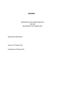
Drivers of extinction risk in African
mammals: the interplay of distribution
state, human pressure, conservation
response and species biology
rstb.royalsocietypublishing.org
Research
Cite this article: Di Marco M, Buchanan GM,
Szantoi Z, Holmgren M, Grottolo Marasini G,
Gross D, Tranquilli S, Boitani L, Rondinini C.
2014 Drivers of extinction risk in African
mammals: the interplay of distribution state,
human pressure, conservation response and
species biology. Phil. Trans. R. Soc. B 369:
20130198.
http://dx.doi.org/10.1098/rstb.2013.0198
One contribution of 9 to a Theme Issue
‘Satellite remote sensing for biodiversity
research and conservation applications’.
Subject Areas:
ecology, environmental science
Keywords:
biodiversity, conservation actions, habitat loss,
life history, random forest model, threats
Author for correspondence:
Moreno Di Marco
e-mail: [email protected]
Electronic supplementary material is available
at http://dx.doi.org/10.1098/rstb.2013.0198 or
via http://rstb.royalsocietypublishing.org.
Moreno Di Marco1, Graeme M. Buchanan2, Zoltan Szantoi3, Milena Holmgren4,
Gabriele Grottolo Marasini1, Dorit Gross3,4, Sandra Tranquilli5, Luigi Boitani1
and Carlo Rondinini1
1
Global Mammal Assessment Program, Department of Biology and Biotechnologies, Sapienza Universita`
di Roma, Viale dell’ Universita` 32, 00185 Rome, Italy
2
Conservation Science, RSPB, 2 Lochside View, Edinburgh EH12 9DH, UK
3
European Commission’s Joint Research Centre, Land Resource Management Unit, Institute for Environment
and Sustainability, Via Enrico Fermi 2749, Ispra 21027, Italy
4
Resource Ecology Group, Wageningen University, PO Box 47, 6700 AA Wageningen, The Netherlands
5
Department of Biological Anthropology, University College London, 14 Taviton Street, London WC1H 0BW, UK
Although conservation intervention has reversed the decline of some species,
our success is outweighed by a much larger number of species moving
towards extinction. Extinction risk modelling can identify correlates of risk
and species not yet recognized to be threatened. Here, we use machine learning models to identify correlates of extinction risk in African terrestrial
mammals using a set of variables belonging to four classes: species distribution state, human pressures, conservation response and species biology.
We derived information on distribution state and human pressure from satellite-borne imagery. Variables in all four classes were identified as important
predictors of extinction risk, and interactions were observed among variables
in different classes (e.g. level of protection, human threats, species distribution ranges). Species biology had a key role in mediating the effect of
external variables. The model was 90% accurate in classifying extinction risk
status of species, but in a few cases the observed and modelled extinction
risk mismatched. Species in this condition might suffer from an incorrect
classification of extinction risk (hence require reassessment). An increased
availability of satellite imagery combined with improved resolution and classification accuracy of the resulting maps will play a progressively greater role in
conservation monitoring.
1. Introduction
The state of biodiversity is deteriorating globally owing to increasing human
pressure and insufficient conservation responses [1], despite considerable
efforts and political engagement from local to global organizations and institutions [2,3]. The drivers of biodiversity decline are multiple (habitat loss,
overhunting, climate change, disease, invasive species, etc.), and affect species
groups differently [4]. Although conservation intervention has slowed down
or reversed the decline of some species, these efforts are outweighed by a
much larger number of species moving towards extinction [5]. For example,
one-quarter of the world’s carnivore and ungulate species have moved closer
to extinction in the past 40 years [6].
Extinction risk analysis has emerged in the past 15 years as a useful analytical tool for providing scientific support to ecologists and conservation biologists
[7]. It has been used to investigate the predictability of species’ extinction
risk from their biological characteristics (i.e. their life-history traits) and their
exposure to threats, mammals often being a model group [8–11]. A number of
& 2014 The Author(s) Published by the Royal Society. All rights reserved.
2. Material and methods
(a) Variables and data sources
We focused our analyses on African terrestrial mammals (figure 1;
electronic supplementary material, figure S1). We assigned
species’ threat status categories (i.e. a proxy of extinction risk)
according to the Red List of the International Union for Conservation of Nature (IUCN) [43]. Following previous approaches [9,13],
we classified all species as being threatened (critically endangered,
endangered, vulnerable) or non-threatened (least concern, near
threatened) depending on their IUCN Red List categories [44],
after removing species classified as data deficient, extinct or extinct
in the wild; a total of 1044 species were included in the analyses.
Twenty three per cent of African mammals are currently threatened with extinction according to the IUCN Red List, a condition
that is comparable with the global figure, where 25% of all
mammal species are threatened [45]. Only species having at least
50% of their global distribution range in Africa were included in
our analyses (all threatened species in the analyses are endemic
to Africa).
2
Phil. Trans. R. Soc. B 369: 20130198
within protected areas (PAs) [34], and African carnivores and
ungulates have faced a continental-scale deterioration in conservation status in the same period [6].
Legislative protection of sites by means of PA networks is
proving effective at reducing forest cover loss [35] and loss of
all natural land cover in African PAs [36]. Net deforestation
rates in Africa have been estimated at 0.14% per year in 2000–
2010 [37], and the rate of vegetation change was generally
faster outside than inside PAs, with some exceptions [38]. A
recent study [39] has demonstrated that long-term presence of
conservation efforts had a significant positive influence on the
persistence of African great apes in 109 PAs. However, conservation resources are limited and need to be substantially increased
[40]. A key step to increase the effectiveness of conservation
action is the identification of clear priorities through robust
analytical methods [41,42]. African mammals represent a promising model group to test a set of interacting correlates of
extinction risk.
We perform an extinction risk analysis to assess the contribution of four classes of potential predictors of extinction risk
in African terrestrial mammals, we measured: (i) species distribution state (e.g. suitable habitat availability and geographical
range size) as the current condition characterizing a species’
distribution; (ii) human pressures (e.g. habitat alteration
within a species’ range) through the use of various satellite
imagery products; (iii) conservation responses (e.g. PA coverage and levels of management in PAs) and (iv) biological
traits (e.g. body mass and weaning age), already known to correlate with mammal extinction risk [11]. We assess the key role
that satellite imagery can play in measuring environmental
condition and change, allowing an improved prediction of
the extinction risk of species.
We use a set of multi-resolution satellite imagery, updated
conservation-relevant information and comprehensive biological characteristics to build our models. We assessed the
relative importance of these drivers and identified multiple
paths of interaction that determine a species’ extinction risk.
We calculate the accuracy of our prediction model in terms of
the proportion of species whose observed extinction risk was
correctly classified, and propose conservation-relevant interpretations for those species with a mismatching classification
in our model.
rstb.royalsocietypublishing.org
different techniques have been used to model the effect
of intrinsic and external variables, including phylogenetic
comparative methods [12], machine learning models [7] and
taxonomically informed generalized linear mixed models [13].
Various extinction risk analyses on mammals have focused
on teasing out the relative importance of biological (i.e. intrinsic) factors in predicting extinction risk [9,11]. Others have
shown that anthropogenic threats are important predictors of
extinction risk too, albeit their relative role in a predictive
model is generally lower relative to biological traits [14,15];
this is perhaps related to the complexity of measuring threat
impact on species compared to measuring species biological
traits [16,17]. The applicability of extinction risk analysis for
practical conservation outcomes can be enhanced by providing
conservation recommendations that are clearly interpretable by
conservation practitioners [18]. Large-scale extinction risk analyses require comprehensive datasets of different types of data.
These include species biological characteristics, distribution
ranges and habitat associations, environmental characteristics
and threats operating within the ranges. Biological characteristics, including reproductive parameters (such as litter size)
and physical traits (such as body mass), are readily available
for groups such as mammals [19,20], but often the datasets
are incomplete (see §2a(iv)).
Assessments of habitat can be hard to gather at a continental scale, and even when they are available there may be
considerable inconsistencies in assessments between sites
[21]. Instead, remote sensing instruments continuously
record large amounts of data concerning land and vegetation
cover, topography and climate, many of them with global
coverage. The data and derived products are increasingly
freely available, providing cost-effective means to collect standardized information relevant to conservation purposes [22].
The usefulness of satellite-derived products in conservation
studies has already been demonstrated. For example, the Normalized Difference Vegetation Index (NDVI) has been used to
test hypotheses on the recent trends in net primary productivity
[23], to relate elephant density and food availability [24], and to
predict habitat suitability for the reintroduction of species
extinct in the wild [25]. The Moderate Resolution Imaging Spectroradiometer (MODIS) and Landsat imagery have been used
in regional and global land cover studies to identify hotspots
of land cover change [26,27], to monitor forest [28,29] and
savannah [30] habitats, to infer their resilience [31] and to
assess the impact of habitat loss on birds [32]. Remote sensing
data have not yet been extensively used in extinction risk modelling, but their improved use has the potential of overcoming
the historical problem of measuring the effect of threats (particularly habitat loss and alteration) on species’ extinction risk
[17]. Most satellite-derived data are available at regular intervals, and can be used to produce assessments of change at
large scales. Satellite imagery can therefore be used to track
changes in environmental conditions owing to anthropogenic
impact, allowing their effect on extinction risk to be modelled.
The African mammalian fauna has been the subject of longstanding scientific attention [33] and comprises some of the
most attractive species for tourists: lion (Pathera leo), leopard,
(P. pardus), African elephant (Loxodonta africana), Cape buffalo
(Syncerus caffer), rhinoceroses (Ceratotherium simum and Diceros
bicornis) and great apes (chimpanzees, Pan troglodytes; bonobos,
P. paniscus; and gorillas, Gorilla gorilla and G. beringei). Nonetheless, it has been estimated that African large mammals
have lost 59% of their populations in the past 40 years even
3
rstb.royalsocietypublishing.org
Phil. Trans. R. Soc. B 369: 20130198
species richness
0
212
Figure 1. Richness of African mammal species (number of species in each 300 m grid cell). See the electronic supplementary material, figure S1 for a colour version.
Following [1,11], we identified four main classes of variables
whose influence on mammals’ extinction risk can be modelled:
species distribution state, human pressure, conservation response
and species biology. For each species, we measured 18 predictor
variables, each belonging to one of the mentioned classes (see
also table 1 for a summary). We overlaid each spatial variable
with each species’ range, and measured a representative value
of the variable for the species (as described in the subsections
below). Spatial quantification of the variables was performed in
GRASS GIS [46].
(i) Distribution state
Variables of distribution state represent the current level of intactness characterizing species distributions. We measured the
size of species geographical ranges from IUCN distribution
range polygons [43]. We also measured the current proportion
of suitable habitat within each species’ range, by using habitat suitability models developed by Rondinini et al. [47]. Habitat
suitability models were based on habitat classifications according to species preferences for land cover types and elevation
range, their tolerance for human disturbance and their water
requirements (at a 300 m spatial resolution).
We used the mean annual NDVI value as a proxy for the current (year 2010) primary productivity within each species’ range,
as also done in previous publications [48]. The NDVI was calculated from composites of satellite imagery (at a 250 m spatial
resolution), by applying the mean compositing method [49] on
1 year of satellite imagery recorded by the MODIS instruments
aboard the Terra and Aqua satellites.
(ii) Human pressure
Variables of human pressure represent the level of anthropogenic
threat affecting biodiversity. We obtained changes in the proportion
of suitable habitat within species’ geographical ranges between 1970
and 2010 (at a 1 km spatial resolution), from [50]. We further estimated, for each species, the net change in mean annual primary
productivity (NDVI, see §2a(i)) and tree cover between 2000 and
2010 (at a 250 m spatial resolution). Tree cover change was calculated
from the MODIS percent tree cover product [51], which quantifies
the percentage of tree cover in any 250 m pixel (see also §2c on the
relationship of this variable with species’ habitat preferences).
We also calculated the proportion of each species’ range overlapping with areas characterized by high values of the human
influence index (HII; at a 1 km spatial resolution) [52,53]. The
HII map was described as ‘the sum total of ecological footprints
of the human population’. It was derived from several different
data sources divided into four main types: population density,
land transformation, accessibility and electrical power infrastructure [52]. We defined high HII values as those being higher than
5, and then tested the effect of an increased threshold value
(HII . 10) following [16].
(iii) Conservation response
Variables of conservation response represent the level of conservation efforts implemented for biodiversity protection. We calculated
the percentage of each species’ range (from 0 to 96% observed)
and the percentage of suitable habitat (from 0 to 81% observed)
overlapping with PAs with IUCN categories I –IV (i.e. those
Table 1. Description of the variables included in the extinction risk modelling. See Material and methods for an extended description of the variables and their
sources.
variable
description
extinction risk
RlThreat
the response variable, binary species threat status (threatened versus non-threatened in the IUCN
Red List)
distribution state
RangeSize
NDVI2010
size of species geographical ranges
mean NDVI value within a species’ range in 2010
SuitPrev
proportion of suitable habitat within a species’ range
conservation
response
species biology
SuitLoss
NDVILossa
net change in the proportion of suitable habitat within a species’ range, between 1970 and 2010
net change in NDVI value within a species’ range, between 2000 and 2010.
TreeCovLossa
HII.5
net change in tree cover percentage within a species’ range, between 2000 and 2010
proportion of a species’ range overlapping with areas having an HII.5
HII.10
AvgCons
proportion of a species’ range overlapping with areas having an HII.10
average amount of conservation actions measured in PAs established within a species’ range
RangeProt
proportion of a species’ range overlapping with PAs
SuitProt
Order
proportion of a species’ suitable habitat overlapping with PAs
taxonomical order
DietBreadth
HabitatBreadth
number of dietary categories eaten by a species
number of habitat layers used by a species
AdultBM
adult body mass
LitterSize
NeonateBM
number of offspring born per litter per female
neonatal body mass
WeaningAge
age when primary nutritional dependency on the mother ends
a
The acronym ‘Loss’ was used to indicate the rationale of the variable, even if the net change in variable values over time was measured (i.e. including losses
and gains).
areas more strictly targeting biodiversity conservation). This was
done by overlaying IUCN range polygons [43] and habitat models
[47] with PA polygons from the world database of PAs [54]. We represented missing-shape PAs (14% of the PAs in Africa totalling 1% of
the African PA surface) with circular polygons, centred on the
reported PAs’ coordinates and having a radius calculated from the
reported PAs’ size. We are aware that representing missing-shape
PAs with a circular buffer may have a (likely minor) influence on
our calculation of species’ PAs coverage [55], but we expect that
this would equally affect all species in our sample.
The level of actual conservation interventions was assessed
from management-related data for a total of 825 African PAs (electronic supplementary material, figure S2). Data on management
levels were collected by Birdlife for important bird areas (IBAs),
many of which are also overlapping with PAs [56] (see §2c on
the rationale for using this dataset). For each site, we considered
the information on implementation of conservation action available in the World Bird Database (WBDB) [56], scored from 0
(very little or no conservation action are in place), 1 (some limited
conservation initiatives are in place), 2 (substantive conservation
measures are being implemented but these are not comprehensive
and are limited by resources and capacity) to 3 (the conservation
measures needed for the site are being comprehensively and
effectively implemented). These data were then merged with
those from Tranquilli et al. [39], who scored levels of conservation intervention for a set of central African PAs characterized
by great apes’ past presence and current presence/absence.
We reconverted the latter dataset according to the WDBD
classification system before merging. For each species, we finally
calculated the average level of conservation action allocated to
PAs for the period 1990–2012.
(iv) Species biology
Biological variables, also referred to as life-history traits, represent
baseline biological characteristics of species. We accounted for
species taxonomy by including order as a categorical variable
[15]. We then used PanTHERIA [19] as a data source for biological
traits. PanTHERIA represents the most comprehensive dataset on
mammalian life-history traits, derived from over 100 000 single
records collected, yet it is characterized by missing data for all
the collected variables. Among all of the available variables, we
selected those for which missing data were completed with the
use of a multiple imputation procedure (as described in [11]), in
order to reduce the effect of data omission in our dataset while
still retaining all species in our sample. The resulting variables
were diet breadth, habitat breadth, adult body mass, litter size,
neonate body mass, weaning age. These variables are a representation of species’ physical characteristics (e.g. body mass) and
life-history speed, along the axes of ‘reproductive timing’ (e.g.
weaning age) and ‘reproductive output’ (e.g. litter size), as
described in [57].
(b) Extinction risk model
We used random forests (RFs) and classification trees (CTs)
to build our model of extinction risk prediction. RF, a machine
learning technique, has been introduced as a supportive tool for
macro-ecological analysis [7]. It has been successfully used in comparative extinction risk analyses for terrestrial [9] and marine [58]
mammals as well as for amphibians [59].
We used RF modelling to test the ability of our variables to
classify threatened and non-threatened African mammals,
based on their IUCN Red List categories [9,59]. RF models
Phil. Trans. R. Soc. B 369: 20130198
human pressure
a
rstb.royalsocietypublishing.org
class
4
Our use of geographical range size as a predictor of extinction
risk may lead to circularity with the IUCN Red List criteria, in
particular criterion B on restricted distribution range [44]. This
issue has previously been resolved by excluding species listed
under criterion B (in the IUCN Red List) from the analyses,
often a substantial proportion of species [9,65,66]. Other
approaches employed to resolve this issue include the use of
indices of relative geographical range decline as proxies of extinction risk [14], or IUCN Red List information on species
population trend [59], rather than Red List categories. Instead
of excluding a large number of species from our analyses (thus
reducing both the representativeness of the sample and the
sample size), we performed two tests, one including range size
as a predictor variable and one excluding it. We verified that a
weak relationship exists between range size and the other external variables in our model (R 2 , 0.05 for all relationships), so
that by excluding range size from the RF model it is likely that
we removed its effect almost entirely. We then followed the classical approach and repeated the analyses after excluding species
listed only under criterion B, to show the consistency among our
models (classification accuracy and variable importance).
Among general variables of habitat suitability and intactness,
we also tested the effect of tree cover change in determining
species’ extinction risk. We are aware that the role of this variable would probably be more influential for forest-dependent
species rather than for savannah and grassland-related species.
(d) Satellite information: testing the effect
of spatial resolution
Several low (30 – 1000 m), medium (4– 30 m) and high (0.6 – 4 m)
spatial resolution optical sensors aboard different satellites provide imagery on a daily (MODIS, AVHRR), or regular basis
(ASTER, Landsat 7-8, MERIS, SPOT 4-5). We clarify that ‘low’
and ‘medium’ resolution are intended here in remote sensing
terms, rather than biological modelling terms. The imagery products from some of these sensors are freely available and are the
preferred choice for many biodiversity and conservation studies.
We tested the effect of using low-resolution satellite imagery
in our analyses. We compared the 250 m resolution MODIS percent tree cover layer with a 30 m resolution Landsat-derived
forest classification. The latter product was obtained from a
classification of Landsat 5 TM and 7 ETMþ imagery, selected
using a web-service platform of the Joint Research Centre of
the European Commission (http://acpobservatory.jrc.ec.europa.
eu/content/land-cover-change). The best available imagery in
the period of 2008 – 2012 was selected for a sample of 47 African
PAs (electronic supplementary material, figure S3) and a 20 km
buffer surrounding each of them (1– 5 Landsat scenes per
PA map were used). Pre-processing of the selected imagery
(radiometric calibration, cloud masking, topographic correction,
de-hazing, radiometric normalization, mosaicing and gap filling)
was based on the methodology described in [68,69].
The original Landsat-derived maps contained the following
classes: cloud/shadow, water, forest, shrubs, grass, bare soil,
burnt and other vegetation. We grouped these classes in a second
step into forest versus non-forest classes, and checked for their consistency visually with the original Landsat imagery (electronic
supplementary material, table S1). Each classified PA map was
then validated to high-resolution imagery by visually comparing
a random selection of 50 points per map (including forested and
non-forested pixels) using Google Earth software (Google Earth).
For each classified PA, we calculated the overall classification
accuracy as well as combined TSS [60], accounting for both sensitivity (correctly classified forested pixels) and specificity (correctly
classified non-forested pixels).
After the validation, we compared for each PA the mean proportion of forest areas derived from Landsat with the value of tree
cover percentage derived from MODIS. Our aim was to verify
whether a linear relationship exists between these two products.
3. Results
(a) Classifying species’ extinction risk
The RF model on the full-species set had high classification
accuracy (93% correctly classified species in the crossvalidation procedure). The model performed well both in
5
Phil. Trans. R. Soc. B 369: 20130198
(c) Addressing limitations in the use of variables
Nonetheless, we believe that the tree cover loss in a certain
area has much broader impacts. In fact, it has been demonstrated
that habitat clearance has contagious effects in forest and grassland [67]. For this reason, we are confident that our measure of
tree cover change is likely to be influential on the extinction
risk of species with diverse habitat preferences.
Measuring the levels of conservation intervention by using
management information collected for IBAs that overlap with
PAs is probably not ideal for our study species. However, this
is one of a very few datasets of management information readily
available at a continental scale and directly related to conservation efforts, as well as a good geographical complement to the
information provided in [39] for central Africa. We used this variable as a proxy of ‘conservation attention’ in PAs, which is
potentially also of broader relevance for mammals.
rstb.royalsocietypublishing.org
combine a series of CTs (n ¼ 500, in our case) based on the predictor variables. Each CT classifies the species through a
recursive binary partitioning that aggregates them into regions
(or ‘nodes’) that are increasingly homogeneous with respect to
their extinction risk. At each step in fitting a CT, an optimization
is carried out to select a node, a predictor variable and a predictor cut-off that result in the most homogeneous subgroups of
species, as measured by the Gini index [7]. In this way, we
could quantify a series of model-related measures of accuracy,
together with relative variables importance and ‘classification
proximity’ among species, as described below.
We measured RF model classification accuracy by calculating
the proportion of correctly classified species (throughout a crossvalidation routine implemented in the RF model). We also verified
the model performance in terms of sensitivity (ability to classify
threatened species correctly) and specificity (ability to classify
non-threatened species correctly). We further calculated K statistics
and true skill statistics (TSS), both weighting overall sensitivity and
specificity performances [60]. We then measured the relative
importance of each variable for the RF model construction. The
importance of each variable in the RF model was measured
through its contribution to: (i) model accuracy for threatened
species, (ii) model accuracy for non-threatened species,
(iii) model accuracy for all species, and (iv) mean decrease in the
Gini index, across the RF trees [61].
Based on the final model classification, we calculated the
classification proximity of species in the RF model, i.e. a measure
of classification similarity between species, calculated from the
number of times in which two species ended up in the same terminal node of the RF trees, during model recursive partitioning. We
used this metric to represent species in a multidimensional scaling
(MDS) analysis (i.e. a principal coordinate analysis). We also investigated the presence of mismatching threat status classifications in
our RF model, i.e. threatened species classified as non-threatened
and vice versa in most of the RF trees.
We then created a single conditional inference CT of classification to evaluate visually a representation of the interaction
between predictor variables in determining pathways of extinction
risk [62]. Statistical analyses, RFs and CTs, were performed in R
[63] using the packages ‘randomForests’ [64] and ‘party’ [62].
a mismatching classification in our RF model (i.e. those
incorrectly classified in the majority of the RF trees).
(c) Interaction among extinction risk predictors
RangeSize
removed
no. species
1044
1044
proportion correctly classified
sensitivity
0.927
0.803
0.900
0.682
specificity
true skill statistic
0.964
0.767
0.965
0.647
K statistic
0.788
0.696
terms of sensitivity (80% of correctly classified threatened
species) and specificity (96% of correctly classified nonthreatened species) (table 2). Overall, both TSS (0.77) and K
statistic (0.79) reported good performances (unity being the
maximum possible in both cases). When removing the variable ‘range size’, the overall model accuracy decreased
slightly (from 0.93 to 0.90), yet model sensitivity and TSS
decreased more substantially (from 0.80 to 0.68 and from
0.77 to 0.65, respectively).
We calculated the importance of each variable according
to four measures, and reported a mean rank value for each
(figure 2a). Range size was the most important variable in our
model. Nonetheless, variables representing each of the four predictor classes (table 1) were all present among the most
important ones. This was observed also when removing
range size as a predictor of extinction risk (figure 2b). Two of
the satellite-derived variables were influential descriptors of
species extinction risk, with both tree cover change and NDVI
2010 coming into the first half of ranked variables in our RF
models (figure 3). In particular, tree cover change was important both in the models with range size (sixth most important
variable) and in the model without range size (third most
important variable).
When repeating the RF analyses on the full set of variables but excluding all threatened species listed only under
criterion B in the IUCN Red List, the degrees of freedom in
our model were reduced to 904 (electronic supplementary
material, table S2). This had little impact on overall RF
model accuracy (still over 90% of species were correctly
classified), but impacted more substantially the model sensitivity (now 0.64). Additionally, this had very little impact on
our variables’ ranking: range size remained the most important variable and eight out of the nine most important
variables remained the same with respect to the full-species
model (electronic supplementary material, figure S4).
(b) Classification proximity
A classical MDS analysis, based on the relative proximity
of each species in each terminal node of the RF, suggested
threatened species are clustered in one ‘arm’ of the coordinate
space, whereas non-threatened species are widely distributed
across the remaining plot area (figure 3). The two clusters are
not discrete, and there is partial overlap between threatened
and non-threatened species. This enabled us to identify
29 non-threatened and 47 threatened species (electronic
supplementary material, tables S3 and S4, respectively) with
A conditional inference CT for the classification of extinction
risk in African mammals (figure 4) showed the complex interaction between multiple predictor variables in different classes.
For example, species having a relatively small distribution
range (less than 11 192 km2) that is substantially covered by
PAs (greater than 24% overlap) but is also largely overlapping
with areas of high human impact (greater than 47% overlap)
face a high probability of being threatened (95%; see pathway
1–15–17–18 in figure 4). In contrast, rodent species with relatively small overlap with PAs (less than 24%) but with a
relatively large distribution range (greater than 23 163 km2)
have a very low probability of being recognized as threatened
with extinction (2%; see pathway 1–2–10–12–14 in figure 4).
(d) The effects of spatial resolution
For a sample of 47 PAs, we classified forest presence according
to Landsat scenes and validated the classification with Google
Earth. The validation process demonstrated good accuracy in
the classification of forested versus non-forested areas in all of
the maps. Proportion of correctly classified pixels, sensitivity
(ability to detect forest areas) and specificity (ability to detect
non-forest area) were all above 85% (table 3). We measured
the correlation between ‘medium-resolution’ satellite imagery
(forest cover from Landsat) and ‘low-resolution’ imagery (tree
cover percentage from MODIS) in our sample PAs. The two satellite products showed a good correlation in our test PAs (linear
model with zero intercept; ß ¼ 1.43, s.e. ¼ 0.13, R 2 ¼ 0.72). On
average, the Landsat classification predicted a higher proportion of forest cover compared with the tree cover
percentage detected by MODIS (figure 5).
4. Discussion
(a) Role of extinction risk predictors
We performed a comprehensive analysis of factors affecting
extinction risk of African mammals and followed Butchart
et al. [1] in considering multiple classes of factors influencing
extinction risk of species. The effects of all these factors are, ultimately, mediated by species biology, which explains why some
species are less prone to endangerment than others, under
similar external conditions. The most important predictors of
extinction risk in our RF model were range size, proportion
of range in PAs, weaning age, neonatal body mass, proportion
of protected suitable area and change in tree cover (figure 2a).
Some of these variables, such as range size or weaning age,
have already been identified as important predictors of
mammals’ extinction risk [15]. Yet, the importance of other
variables, such as the change in tree cover as assessed from
remote sensing, are identified here for the first time. Collecting
tree cover data at a continental scale using methods other than
remote sensing would be impossible. Although monitoring
land cover changes automatically at continental scales remains
challenging [70], our results here highlight one of the potential
future application of global change data from satellites (see also
[29]) in conservation-related analyses.
The level of protection (both referring to the presence of
PAs within species ranges and within suitable habitat in the
Phil. Trans. R. Soc. B 369: 20130198
parameter
all
variables
6
rstb.royalsocietypublishing.org
Table 2. Performance statistics of the RF classification model. Both the
performance of the full model and the performance of the model without
the range size variable are reported.
(a)
(b)
7
RangeSize
RangeProt
SuitProt
TreeCovLoss
NeonateBM
NeonateBM
SuitProt
WeaningAge
TreeCovLoss
Order
AdultBM
rstb.royalsocietypublishing.org
RangeProt
WeaningAge
NDVI2010
Order
AdultBM
NDVI2010
AvgCons
Phil. Trans. R. Soc. B 369: 20130198
HII.5
HII.5
AvgCons
SuitPrev
HII.10
HII.10
LitterSize
SuitPrev
LitterSize
SuitLoss
NDVILoss
NDVILoss
SuitLoss
DietBreadth
HabitatBreadth
HabitatBreadth
DietBreadth
1
3
5
7 9
12
mean rank
15
18
1
3
5
7 9 11
mean rank
14
17
Figure 2. Relative importance of each predictor variable included in the RF model. The importance of each variable was estimated according to four measures (see
§2). Variables were ranked according to their importance for each measure and a final mean rank was calculated and reported. All variables were tested in (a), while
range size was removed before the test in (b). See table 1 for a description of the variables.
coordinate 2
0.4
0.2
0
–0.2
–0.4
–0.2
0
coordinate 1
0.2
0.4
Figure 3. Classical MDS of African mammals based on their ‘classification proximity’ in the full RF model (all variables included). See §2b,c for analytical details.
Black circles denote threatened and grey circles denote non-threatened species.
ranges) was an important predictor in our model. The establishment of PAs has often been related to the protection of
charismatic species [71], which are generally large-bodied,
characterized by relatively slow life histories and affected
by a variety of threats ( particularly habitat loss and hunting).
Our results suggest a link between establishment of PAs
and retention of a non-threatened status for mammals, yet
we could not fully explain whether this is due to the role of
the PAs in reducing habitat loss or other conservation
benefits linked to the PA, such as reduced poaching and
lower human disturbance.
The level of conservation effort in PAs did not have a strong
effect in our model. This may depend on the fact that the information on conservation efforts was not properly defined to
be effectively linked to the conservation status of our study
species. Although we expected that the conservation efforts
data referred to important bird areas overlapping with PAs
could potentially be a broad proxy of conservation attention,
these data might not necessarily have a direct relevance for
mammals. Additionally, it is likely that, at the scale of our
analyses, the presence of the PAs inside the whole distribution range of a species is more important than the relative
levels of conservation efforts. Recent large- and local-scale
studies have demonstrated the crucial role of the different
conservation efforts on species protection inside PAs [4,39].
Improving the availability of conservation interventions data,
both inside and outside PAs, is strategic, since this has a potential to improve our understanding of the complex relationship
between threats–traits–conservation efforts.
(i) The role of geographical range size
The use of range size as a predictor of species threat status,
derived from IUCN Red List, may lead to model circularity.
8
1
RangeProt
15
Order
Hll.10
AFROSORICIDA, PERISSODACTYLA,
PRIMATES, PROBOSCIDEA
OTHERS
17
RangeSize
WeaningAge
RangeSize
£125
>125
10
RangeSize
> 479 803
£ 479 803
£11 192
>11 192
12
CARNIVORA,
CETARTIODACTYLA, OTHERS
LAGOMORPHA,
MACROSCELIDEA
WeaningAge
£418
>418
0
0
0
0
0
0
0
0
prop. threatened
prop. threatened
prop. threatened
prop. threatened
prop. threatened
prop. threatened
prop. threatened
prop. threatened
prop. threatened
node 4 n = 45 node 6 n = 170 node 7 n = 546 node 9 n = 71 node 11 n = 51 node 13 n = 28 node 14 n = 7 node 16 n = 19 node 18 n = 100 node 19 n = 7
1
1
1
1
1
1
1
1
1
0
0
Figure 4. Conditional inference CT for African mammals. Each terminal node reports (in dark grey) the proportion of included threatened species.
Table 3. Results of the visual ground-truthing validation of the forest cover
in 43 African PAs (and surrounding buffer) as classified by interpretation of
the Landsat TM scenes. For each map, 50 random points (including forest
and non-forest) were extracted and visually compared with Google Earth
imagery. Separate statistics are reported for each area. It was not possible
to validate four additional maps, owing to the excessive presence of clouds.
parameter
value
no. areas
43
proportion correctly classified
specificity
0.91 (s.d. 0.08)
0.89 (s.d. 0.12)
sensitivity
0.86 (s.d. 0.22)
true skills statistic
0.72 (s.d. 0.23)
In fact, range size is used in the IUCN Red List assessment to
apply the criterion B on restricted distribution [44]. Yet,
restricted distribution is not itself sufficient to trigger criterion
B, and other conditions (such as severe fragmentation or ongoing population decline) must also be met at once to qualify
a species as threatened in the Red List. Nonetheless, various
methods have been proposed to avoid having potential circularity in the use of range size as a model predictor (see §2c).
We tested our RF model on the whole set of predictor
variables, and then removed range size to repeat the test.
Additionally, we repeated the analyses after excluding
those threatened species listed only under criterion B. Our
comparisons critically showed that in all of our tests the overall accuracy and, most importantly, the sensitivity of the RF
models were higher with respect to previously published
extinction risk analyses on mammals (e.g. [9]). Nonetheless,
removing species listed only under criterion B or removing
range size from the variables reduced the ability to classify
threatened species correctly. In all tests, our measure of relative importance of variables confirmed that: (i) all of the four
different classes of variables were influential in predicting
extinction risk, (ii) the three RF models shared seven out of
the nine most influential predictors of extinction risk (with
only small changes in their ranked importance), (iii) range
size was the most important predictor even after removing
species listed only under criterion B, as also found in [65].
We acknowledge that the use of IUCN range polygons to
represent species distribution is probably subjected to potential errors and gaps in the data (e.g. [72]), yet this is the most
updated data source available for mammals (as well as many
other groups) globally. We thus stress the importance of
maintaining and ensuring a constant update and refinement
of this key information.
(ii) Using satellite imagery in extinction risk analysis
In our models, we tested the effect of multiple satellite-derived
maps of habitat state and habitat change (i.e. human pressure).
Previous extinction risk analyses have generally considered a
limited number of external correlates (especially threats) with
respect to intrinsic (biological) correlates. This is perhaps
related to the uncertainty affecting threat measurement, and
limited data availability [16,17]. Our results suggest that an
increased use of satellite imagery can contribute to enhancing
our understanding of how multiple factors drive species’
extinction risk at a large scale.
Remote sensing is a powerful and increasingly available
technology in conservation. Its tools and applications provide
opportunities to monitor changes in the conservation status
of threatened species in areas impacted by habitat conversion
[32] and can inform the classification of species’ extinction
Phil. Trans. R. Soc. B 369: 20130198
>23 163
5
Order
prop. threatened
>0.467
8
£23 163
1
£0.467
3
rstb.royalsocietypublishing.org
>0.239
£ 0.239
2
9
Landsat
60
40
R2 = 0.72
bisector
20
0
0
20
40
60
80
100
Figure 5. Comparison of the 2010 percentage of forest cover in a sample of African PAs (and surrounding buffer). The solid line represents the linear fit (with zero
intercept) between the Landsat maps and the MODIS maps, whereas the dashed line is the bisector ( y ¼ x). The sampled areas were the same as in table 3.
risk, thus reducing the problem of outdated assessments in
the IUCN Red List [73] (see §4b).
Satellite imagery is available from a variety of sources;
however, the spatial and temporal resolutions, as well as its
cost, determine its applications. In our extinction risk analysis,
we used a series of satellite-derived products from freely available sources, with spatial resolutions ranging from 250 m (for
MODIS) to 1000 m (for the HII composite map). We also
showed that the classification of medium-resolution (30 m)
Landsat imagery produced reliable maps of forest cover for a
sample of African PAs. The Landsat-derived forest cover was
also well correlated with a MODIS-derived tree cover product
(250 m), one of the most important predictors in our model. A
higher spatial accuracy is now being reached in the classification of forest cover change at a global scale [29], thus
improving our ability to track local drivers of habitat alteration,
such as non-industrial logging.
Our analysis illustrates the value of stronger links between
the remote sensing and the conservation scientific communities. Our extinction risk models benefitted from the use of
satellite-derived assessments of land cover condition and
forest change. Regular updates of both, and other land cover
variables, could contribute to more accurate extinction risk
modelling in the future; however, remote sensing specialists
are needed to produce the tools to undertake these large-scale
assessments and validations.
(b) Classification proximity and mismatching
classifications
In an MDS analysis, based on the frequency that pairs of
species are in the same terminal nodes of our RF model,
threatened species were generally clustered together and overlapped only partially with non-threatened species, which were
instead spread across the remaining coordinate space. This is
probably due to the fact that threshold levels of extinction
risk (i.e. characterizing threatened species in the IUCN Red
List) arise only when a limited set of conditions are met (e.g.
high threats and slow life history). This is also likely related
to the spatial (i.e. biogeographic) and evolutionary signal in
extinction risk [48].
Twenty nine non-threatened species (electronic supplementary material, table S3) were misclassified as threatened
in our RF model (i.e. they are represented in the ‘high-risk’
branch of figure 3). This could be an effect of the model
being unable to consider some of the factors potentially mitigating threats impact on species. However, an alternative
explanation is that the current IUCN assessment for these
species may be erroneous and needs review, and some of
the currently non-threatened species are facing conditions
that may result in a substantial increase in their extinction
risk in the near future. In this latter case, our results are
pinpointing species in potential need of increased conservation attention. Incorrectly classified non-threatened species
in our model mostly included small mammals (such as the
near threatened Zambian mole rat, Cryptomys anselli) and primates (such as the aye-aye, Daubentonia madagascariensis,
which was until recently classified as endangered), but also
included the white rhinoceros, Ceratotherium simum, a charismatic species that suffers from high levels of poaching
(something with no direct surrogate in our current analysis)
despite receiving substantial conservation attention [74].
These species should be carefully considered for future
reassessments of their conservation status in the IUCN
Red List. We believe that a wider (both taxonomically
and spatially) application of our method can provide an
important tool for Red List (re-)assessments [73].
On the other hand, 47 threatened species (electronic
supplementary material, table S4) were misclassified as
non-threatened in our RF model (i.e. they are not represented
in the ‘high-risk’ branch of figure 3). A likely explanation for
this mismatch is that we were not able to consider all of the
threatening factors affecting mammal species extinction risk
in Africa. In fact, our use of satellite imagery allowed us to
consider a set of habitat loss-related drivers (such as the
loss of tree cover), while we could only approximate (e.g.
through the use of HII) harvest-related threats, such as persecution, poaching and bushmeat consumption. Direct kill (in
its various forms) is a key driver of extinction risk for
mammal species globally [75] and is particularly severe for
African mammals [76]. Many of the threatened species with
a mismatching classification in our model are known to be
persecuted by locals as a preventive measure (or as a retaliation) for livestock predation (e.g. the lion, Panthera leo), while
others are poached for their horns (e.g. the black rhino,
Diceros bicornis) [74], or are killed for their meat at unsustainable levels (e.g. Dorcas gazelle, Gazella dorcas) [43]. Other
threatened species in this group are affected by a combination
of direct kill and other drivers not included in our model, e.g.
the western gorilla (Gorilla gorilla) population is facing a rapid
decline owing to commercial hunting and spread of the Ebola
virus [77]. Despite providing a clear improvement in resolution (for extinction risk analysis), habitat variables in our
model are likely to be significant at the landscape scale. On
Phil. Trans. R. Soc. B 369: 20130198
MODIS
rstb.royalsocietypublishing.org
80
(c) Interaction among extinction risk correlates
10
The current extinction risk in African mammal species can
largely be explained by the combined effect of multiple
correlates. The type and dimension of responses of species
to human disturbances and conservation actions are determined by their biology. Our work illustrates how the use of
multiple satellite imagery sources can improve our ability
to track external drivers of extinction risk. Our results suggest
that conservation interventions (e.g. establishment of PAs)
are beneficial in reducing species’ extinction risk, provided
that a combination of biological and external conditions is
verified. This evaluation is of practical significance, as advocated by Cardillo & Meijaard [18], because conservation
planners can use our results as a guideline to improve the
allocation of conservation resources.
Our method can have broader applications, both for other
regions and for other taxa, and its application of extinction
risk analysis to inform Red List reassessments has great potential. We envisage that an increased availability of freely
accessible satellite data as well as an improved resolution and
classification accuracy of the resulting maps will play a substantial role in future conservation monitoring and will increasingly
be part of an enhanced toolbox for conservation scientists.
Acknowledgements. We thank Dr Kamran Safi and two anonymous
reviewers for providing comments that greatly improved our manuscript. We are grateful to several people for their help with the data
processing. Michael Evans at Birdlife International manages the
WBDB, which is compiled with data submitted by many individuals.
Jean-Franc¸ois Pekel and Marco Clerici at the Joint Research Centre of
the European Union (JRC) provided the annual MODIS composites,
baseline data for the calculation of NDVI. Dario Simonetti and
Andreas Brink at JRC helped process the Landsat imagery. Piero Visconti at Microsoft Research provided data on the change in suitable
habitat for the species. Habitat suitability models were developed
in the Global Mammal Assessment Laboratory, Sapienza University
of Rome, based on data provided by many individuals involved
with the IUCN Red List.
References
1.
2.
3.
4.
5.
6.
Butchart SHM et al. 2010 Global biodiversity:
indicators of recent declines. Science 328,
1164–1168. (doi:10.1126/science.1187512)
Convention on Biological Diversity 2011 COP
Decision X/2: Strategic plan for biodiversity
2011 –2020.
United Nations 2008 Millennium Development Goals
Indicators.
Laurance WF et al. 2012 Averting biodiversity
collapse in tropical forest protected areas. Nature
489, 290–294. (doi:10.1038/nature11318)
Hoffmann M et al. 2010 The impact of conservation
on the status of the world’s vertebrates.
Science 330, 1503 –1509. (doi:10.1126/
science.1194442)
Di Marco M, Boitani L, Mallon L, Hoffmann M,
Iacucci A, Meijaard E, Visconti P, Schipper J,
Rondinini C. In press. A retrospective evaluation of
the global decline of carnivores and ungulates.
Conserv. Biol. (doi:10.1111/cobi.12249)
7.
Cutler DR, Edwards TC, Beard KH, Cutler A, Hess KT,
Gibson J, Lawler JJ. 2007 Random forests for
classification in ecology. Ecology 88, 2783–2792.
(doi:10.1890/07-0539.1)
8. Cardillo M, Mace GM, Jones KE, Bielby J, BinindaEmonds ORP, Sechrest W, Orme CDL, Purvis A. 2005
Multiple causes of high extinction risk in large
mammal species. Science 309, 1239– 1241. (doi:10.
1126/science.1116030)
9. Davidson AD, Hamilton MJ, Boyer AG, Brown JH,
Ceballos G. 2009 Multiple ecological pathways to
extinction in mammals. Proc. Natl Acad. Sci. USA 106,
10 702–10 705. (doi:10.1073/pnas.0901956106)
10. Bielby J, Cardillo M, Cooper N, Purvis A. 2010
Modelling extinction risk in multispecies data sets:
phylogenetically independent contrasts versus
decision trees. Biodivers. Conserv. 19, 113– 127.
(doi:10.1007/s10531-009-9709-0)
11. Di Marco M, Cardillo M, Possingham HP, Wilson KA,
Blomberg SP, Boitani L, Rondinini C. 2012 A novel
12.
13.
14.
15.
approach for global mammal extinction risk reduction.
Conserv. Lett. 5, 134–141. (doi:10.1111/j.1755-263X.
2011.00219.x)
Purvis A. 2008 Phylogenetic approaches to the
study of extinction. Annu. Rev. Ecol. Evol. Syst. 39,
301–319. (doi:10.1146/annurev.ecolsys.063008.
102010)
Gonza´lez-Sua´rez M, Revilla E. 2013 Variability in
life-history and ecological traits is a buffer against
extinction in mammals. Ecol. Lett. 16, 242 –251.
(doi:10.1111/ele.12035)
Fisher DO, Blomberg SP, Owens IPF. 2003 Extrinsic
versus intrinsic factors in the decline and extinction
of Australian marsupials. Proc. R. Soc. Lond. B 270,
1801– 1808. (doi:10.1098/rspb.2003.2447)
Cardillo M, Mace GM, Gittleman JL, Jones KE, Bielby
J, Purvis A. 2008 The predictability of extinction:
biological and external correlates of decline in
mammals. Proc. R. Soc. B 275, 1441– 1448.
(doi:10.1098/rspb.2008.0179)
Phil. Trans. R. Soc. B 369: 20130198
Our analysis demonstrates that there are multiple routes to
extinction (figure 4). In all the described paths, interacting factors determine large changes in the probability of a species to
be threatened. For example, all other conditions being similar
(taxonomy, range size, level of protection), species characterized by a weaning age longer than 418 days are substantially
more likely to be threatened than those with a lower weaning
age value (figure 4, terminal nodes 8 and 9). Similarly, species
characterized by a significant level of protection but facing high
levels of human impact (e.g. outside PAs) may have a high or
moderate probability of being threatened with extinction,
depending on their range size being smaller or larger than
11 000 km2 (figure 4, terminal nodes 18 and 19). Interestingly,
this same range size threshold has been already been identified
as a good predictor of threatened birds [78].
Candidate variables in our RF model correctly predicted
the extinction risk of over 80% of both threatened and nonthreatened species (i.e. high sensitivity and high specificity).
Our results demonstrate the combined effect of multiple classes
of drivers in shaping the current extinction risk of African
mammals. In previous extinction risk analyses [15,58], biological factors played a central role in explaining model variance,
whereas external factors were generally less relevant. We
showed that using a number of satellite-derived measures of
human pressures and distribution state changes the situation.
Our measures of relative variable importance highlighted
that both biological and external factors are included among
the top-ranked variables in all our models (figure 2).
5. Conclusion
rstb.royalsocietypublishing.org
the other hand, threatened small-bodied species incorrectly
classified in our model (i.e. some bats and rodents) may
also respond to finer scale habitat modification. As already
mentioned, it is also possible that the status of some of the
incorrectly classified threatened species in our model needs
to be reassessed in the IUCN Red List, again highlighting a
potential use of the proposed approach [73].
31.
32.
34.
35.
36.
37.
38.
39.
40.
41.
42.
43.
44.
45. Schipper J et al. 2008 The status of the world’s
land and marine mammals: diversity, threat, and
knowledge. Science 322, 225–230. (doi:10.1126/
science.1165115)
46. GRASS Development Team 2010 Open source
GIS.Software, Version 6.4.0. Open Source Geospatial
Foundation.
47. Rondinini C et al. 2011 Global habitat suitability
models of terrestrial mammals. Phil. Trans. R. Soc. B
366, 2633– 2641. (doi:10.1098/rstb.2011.0113)
48. Safi K, Pettorelli N. 2010 Phylogenetic, spatial and
environmental components of extinction risk in
carnivores. Glob. Ecol. Biogeogr. 19, 352 –362.
(doi:10.1111/j.1466-8238.2010.00523.x)
49. Vancutsem C, Pekel JF, Bogaert P, Defourny P. 2007
Mean compositing, an alternative strategy for
producing temporal syntheses. Concepts and
performance assessment for SPOT VEGETATION time
series. Int. J. Remote Sens. 28, 5123–5141. (doi:10.
1080/01431160701253212)
50. Visconti P et al. 2011 Future hotspots of terrestrial
mammal loss. Phil. Trans. R. Soc. B 366,
2693– 2702. (doi:10.1098/rstb.2011.0105)
51. Hansen MC, DeFries RS, Townshend JRG, Carroll M,
Dimiceli C, Sohlberg RA. 2003 Global percent tree
cover at a spatial resolution of 500 meters: first
results of the MODIS Vegetation Continuous
Fields Algorithm. Earth Interact. 7, 1–15. (doi:10.
1175/1087-3562(2003)007,0001:GPTCAA.2.0.
CO;2)
52. Sanderson EW, Jaiteh M, Levy MA, Redford KH,
Wannebo AV, Woolmer G. 2002 The human
footprint and the last of the wild. Bioscience 52,
891–904. (doi:10.1641/0006-3568(2002)052
[0891:THFATL]2.0.CO;2)
53. Wildlife Conservation Society (WCS) & Center for
International Earth Science Information Network
(CIESIN) 2005 Last of the Wild Project, Version 2,
2005 (LWP-2): Global Human Footprint Dataset. See
http://sedac.ciesin.columbia.edu/data/set/wildareasv2-human-footprint-geographic.
54. United Nations Environment Programme–World
Conservation Monitoring Centre 2012 The world
database on protected areas (WDPA). Cambridge,
UK: UNEP-WCMC.
55. Visconti P, Di Marco M, A´lvarez-Romero JG,
Januchowski-Hartley SR, Pressey RL, Weeks R,
Rondinini C. 2013 Effects of errors and gaps in
spatial data sets on assessment of conservation
progress. Conserv. Biol. 27, 1000– 1010.
56. Birdlife International 2012 The World Bird Database.
See http://www.birdlife.org/action/science/
knowledge_management/index.html.
57. Bielby J, Mace GM, Bininda-Emonds ORP, Cardillo
M, Gittleman JL, Jones KE, Orme CDL, Purvis A.
2007 The fast–slow continuum in mammalian life
history: an empirical reevaluation. Am. Nat. 169,
748–757. (doi:10.1086/516847)
58. Davidson AD, Boyer AG, Kim H, Pompa-Mansilla S,
Hamilton MJ, Costa DP, Ceballos G, Brown JH.
2012 Drivers and hotspots of extinction risk in
marine mammals. Proc. Natl Acad. Sci. USA 108,
13 600 –13 605.
11
Phil. Trans. R. Soc. B 369: 20130198
33.
and MODIS imagery. J. Nat. Conserv. 18, 169– 179.
(doi:10.1016/j.jnc.2009.08.001)
Hirota M, Holmgren M, Van Nes EH, Scheffer M.
2011 Global resilience of tropical forest and savanna
to critical transitions. Science 334, 232–235.
(doi:10.1126/science.1210657)
Buchanan GM, Butchart SHM, Dutson G, Pilgrim JD,
Steininger MK, Bishop KD, Mayaux P. 2008 Using
remote sensing to inform conservation status
assessment: estimates of recent deforestation rates
on New Britain and the impacts upon endemic
birds. Biol. Conserv. 141, 56 –66. (doi:10.1016/j.
biocon.2007.08.023)
Trimble MJ, van Aarde RJ. 2010 Species inequality
in scientific study. Conserv. Biol. 24, 886–890.
(doi:10.1111/j.1523-1739.2010.01453.x)
Craigie ID, Baillie JEM, Balmford A, Carbone C,
Collen B, Green RE, Hutton JM. 2010 Large mammal
population declines in Africa’s protected areas. Biol.
Conserv. 143, 2221–2228. (doi:10.1016/j.biocon.
2010.06.007)
Geldmann J, Barnes M, Coad L, Craigie ID,
Hockings M, Burgess ND. 2013 Effectiveness of
terrestrial protected areas in reducing habitat loss
and population declines. Biol. Conserv. 161,
230 –238. (doi:10.1016/j.biocon.2013.02.018)
Beresford AE et al. 2013 Protection reduces loss of
natural land-cover at sites of conservation
importance across Africa. PLoS ONE 8, e65370.
(doi:10.1371/journal.pone.0065370)
Mayaux P et al. 2013 State and evolution of the
African rainforests between 1990 and 2010. Phil.
Trans. R. Soc. B 368, 20120300. (doi:10.1098/
rstb.2012.0300)
Wegmann M, Santini L, Leutner B, Safi K,
Rocchini D, Bevanda M, Latifi H, Dech S, Rondinini C.
2014 Role of African protected areas in maintaining
connectivity for large mammals. Phil. Trans. R. Soc. B
369, 20130193. (doi:10.1098/rstb.2013.0193)
Tranquilli S et al. 2012 Lack of conservation effort
rapidly increases African great ape extinction risk.
Conserv. Lett. 5, 48– 55. (doi:10.1111/j.1755-263X.
2011.00211.x)
McCarthy DP et al. 2012 Financial costs of meeting
global biodiversity conservation targets: current
spending and unmet needs. Science 338, 946–949.
(doi:10.1126/science.1229803)
Rondinini C, Rodrigues ASL, Boitani L. 2011
The key elements of a comprehensive
global mammal conservation strategy. Phil.
Trans. R. Soc. B 366, 2591–2597. (doi:10.1098/
rstb.2011.0111)
Rondinini C et al. 2011 Reconciling global mammal
prioritization schemes into a strategy. Phil.
Trans. R. Soc. B 366, 2722–2728. (doi:10.1098/
rstb.2011.0112)
International Union for Conservation of Nature 2012
IUCN Red List of Threatened Species Version 2012.1.
See http://www.iucnredlist.org.
International Union for Conservation of Nature
Species Survival Commission 2001 IUCN Red List
categories and criteria, version 3.1. Cambridge, UK:
IUCN.
rstb.royalsocietypublishing.org
16. Di Marco M, Rondinini C, Boitani L, Murray KA. 2013
Comparing multiple species distribution proxies and
different quantifications of the human footprint
map, implications for conservation. Biol. Conserv.
165, 203–211. (doi:10.1016/j.biocon.2013.05.030)
17. Murray KA, Verde Arregoitia LD, Davidson A, Di
Marco M, Di Fonzo MMI. 2014 Threat to the point:
improving the value of comparative extinction risk
analysis for conservation action. Glob. Chang. Biol.
20, 483–494. (doi:10.1111/gcb.12366)
18. Cardillo M, Meijaard E. 2012 Are comparative
studies of extinction risk useful for conservation?
Trends Ecol. Evol. 27, 167 –171. (doi:10.1016/j.tree.
2011.09.013)
19. Jones KE et al. 2009 PanTHERIA: a species-level
database of life history, ecology, and geography of
extant and recently extinct mammals. Ecology 90,
2648. (doi:10.1890/08-1494.1)
20. Tacutu R, Craig T, Budovsky A. 2013 Human ageing
genomic resources: integrated databases and tools
for the biology and genetics of ageing. Nucleic Acids
Res. 41, 1027 –1033. (doi:10.1093/nar/gks1155)
21. Buchanan GM, Fishpool LDC, Evans MI, Butchart
SHM. 2013 Comparing field-based monitoring and
remote-sensing, using deforestation from logging at
Important Bird Areas as a case study. Biol. Conserv.
167, 334–338. (doi:10.1016/j.biocon.2013.08.031)
22. Turner W. 2013 Satellites: make data freely
accessible. Nature 498, 37. (doi:10.1038/498037c)
23. Pettorelli N, Chauvenet ALM, Duffy JP, Cornforth
WA, Meillere A, Baillie JEM. 2012 Tracking the effect
of climate change on ecosystem functioning using
protected areas: Africa as a case study. Ecol. Indic.
20, 269–276. (doi:10.1016/j.ecolind.2012.02.014)
24. Duffy J, Pettorelli N. 2012 Exploring the relationship
between NDVI and African elephant population
density in protected areas. Afr. J. Ecol. 50,
455–463. (doi:10.1111/j.1365-2028.2012.01340.x)
25. Freemantle TP, Wacher T, Newby J, Pettorelli N.
2013 Earth observation: overlooked potential to
support species reintroduction programmes.
Afr. J. Ecol. 51, 482–492. (doi:10.1111/aje.12060)
26. Sa´nchez-Cuervo AM, Aide TM, Clark ML, Etter A.
2012 Land cover change in Colombia: surprising
forest recovery trends between 2001 and 2010. PLoS
One 7, e43943. (doi:10.1371/journal.pone.0043943)
27. Wessels K. 2004 Mapping regional land cover with
MODIS data for biological conservation: examples
from the Greater Yellowstone Ecosystem, USA and
Para´ State, Brazil. Remote Sens. Environ. 92, 67– 83.
(doi:10.1016/j.rse.2004.05.002)
28. Broich M, Hansen MC, Potapov P, Adusei B,
Lindquist E, Stehman SV. 2011 Time-series analysis
of multi-resolution optical imagery for quantifying
forest cover loss in Sumatra and Kalimantan,
Indonesia. Int. J. Appl. Earth Obs. Geoinf. 13,
277–291. (doi:10.1016/j.jag.2010.11.004)
29. Hansen MC et al. 2013 High-resolution global maps
of 21st-century forest cover change. Science 342,
850–853. (doi:10.1126/science.1244693)
30. Munyati C, Ratshibvumo T. 2010 Differentiating
geological fertility derived vegetation zones in
Kruger National Park, South Africa, using Landsat
73.
74.
75.
76.
77.
78.
of the robustness of global amphibian range
maps. J. Biogeogr. 41, 211–221. (doi:10.1111/
jbi.12206)
Rondinini C, Di Marco M, Visconti P, Butchart S,
Boitani L. In press. Update or outdate: long term
viability of the IUCN Red List. Conserv. Lett. (doi:10.
1111/conl.12040)
Biggs D, Courchamp F, Martin R, Possingham H.
2013 Legal trade of Africa’s rhino horns.
Science 339, 1038– 1039. (doi:10.1126/science.
1229998)
Hoffmann M, Belant JL, Chanson JS, Cox NA,
Lamoreux J, Rodrigues ASL, Schipper J, Stuart SN.
2011 The changing fates of the world’s mammals.
Phil. Trans. R. Soc. B 366, 2598–2610. (doi:10.
1098/rstb.2011.0116)
Milner-Gulland EJ, Bennett EL. 2003 Wild meat: the
bigger picture. Trends Ecol. Evol. 18, 351 –357.
(doi:10.1016/S0169-5347(03)00123-X)
Walsh PD et al. 2003 Catastrophic ape decline in
western equatorial Africa. Nature 422, 611 –614.
(doi:10.1038/nature01566)
Harris G, Pimm SL. 2008 Range size and
extinction risk in forest birds. Conserv. Biol.
22, 163 –171. (doi:10.1111/j.1523-1739.2007.
00798.x)
12
Phil. Trans. R. Soc. B 369: 20130198
67. Boakes EH, Mace GM, McGowan PJK, Fuller RA.
2010 Extreme contagion in global habitat clearance.
Proc. R. Soc. B 277, 1081–1085. (doi:10.1098/rspb.
2009.1771)
68. Bodart C, Eva H, Beuchle R, Rasˇi R, Simonetti D,
Stibig H-J, Brink A, Lindquist E, Achard F. 2011
Pre-processing of a sample of multi-scene and
multi-date Landsat imagery used to monitor
forest cover changes over the tropics. ISPRS
J. Photogramm. Remote Sens. 66, 555–563.
(doi:10.1016/j.isprsjprs.2011.03.003)
69. Szantoi Z, Simonetti D. 2013 Fast and robust
topographic correction method for medium resolution
satellite imagery using a stratified approach. IEEE
J. Sel. Top. Appl. Earth Obs. Remote Sens. 6,
1921–1933. (doi:10.1109/JSTARS.2012.2229260)
70. Gross D, Dubois G, Pekel J-F, Mayaux P, Holmgren
M, Prins HHT, Rondinini C, Boitani L. 2013
Monitoring land cover changes in African protected
areas in the 21st century. Ecol. Inform. 14, 31 –37.
(doi:10.1016/j.ecoinf.2012.12.002)
71. Walpole M, Leader-Williams N. 2002 Tourism and
flagship species in conservation. Biodivers. Conserv.
11, 543– 547. (doi:10.1023/A:1014864708777)
72. Ficetola GF, Rondinini C, Bonardi A, Katariya V,
Padoa-Schioppa E, Angulo A. 2014 An evaluation
rstb.royalsocietypublishing.org
59. Murray KA, Rosauer D, McCallum H, Skerratt LF.
2011 Integrating species traits with extrinsic threats:
closing the gap between predicting and preventing
species declines. Proc. R. Soc. B 278, 1515 –1523.
(doi:10.1098/rspb.2010.1872)
60. Allouche O, Tsoar A, Kadmon R. 2006 Assessing the
accuracy of species distribution models: prevalence,
kappa and the true skill statistic (TSS). J. Appl. Ecol. 43,
1223–1232. (doi:10.1111/j.1365-2664.2006.01214.x)
61. Breiman L. 2001 Random forests. Berkeley, CA:
University of California.
62. Strobl C, Hothorn T, Zeileis A. 2009 Party on. R J. 1,
14 –17.
63. R Development CoreTeam. 2011 R: a language and
environment for statistical computing. Vienna,
Austria. (http://www.R-project.org/)
64. Liaw A, Wiener M. 2002 The randomforest package.
R News 2, 18 –22.
65. Purvis A, Gittleman JL, Cowlishaw G, Mace GM.
2000 Predicting extinction risk in declining species.
Proc. R. Soc. Lond. B 267, 1947 –1952. (doi:10.
1098/rspb.2000.1234)
66. Cardillo M, Mace GM, Gittleman JL, Purvis A. 2006
Latent extinction risk and the future battlegrounds
of mammal conservation. Proc. Natl Acad. Sci. USA
103, 4157 –4161. (doi:10.1073/pnas.0510541103)