
CEP Discussion Paper No 1349 May 2015 Space
ISSN 2042-2695 CEP Discussion Paper No 1349 May 2015 Space-Time (In)Consistency in the National Accounts: Causes and Cures Nicholas Oulton Abstract In early 2014 the World Bank published the main findings of the 2011 International Comparison Program (ICP). The result was surprising: the world is apparently richer and more equal than we would have expected based on extrapolating from the earlier, 2005 ICP. This is an example of what I call space-time inconsistency in the national accounts. Though the 2011 findings drew attention to this problem, it is certainly present in earlier rounds of the ICP, for example in comparing the 1980 with the 2005 ICP. In this paper I show that the national accounts are in principle space-time consistent if the consumer’s utility function (or the revenue (GDP) function) is homothetic and if Divisia price indices are used to deflate nominal GDP or consumption, both over time and across countries. It follows that any observed inconsistency must be due to either (a) non-homotheticity in consumption (or production); (b) approximation error when discrete chain indices are used instead of continuous Divisia indices; or (c) errors in domestic price indices and PPPs. I develop indicators of the size of non-homotheticity and chain index approximation error using detailed, unpublished data from the 2005 ICP. I conclude that errors in price indices are most likely the major cause of inconsistency. Keywords: PPP, Divisia, Konüs, price index, path-dependence, consistency JEL codes: C43; O47; I31; F43 This paper was produced as part of the Centre’s Productivity Programme. The Centre for Economic Performance is financed by the Economic and Social Research Council. An earlier version of this paper was presented to the 33rd General Conference of the International Association for Research in Income and Wealth, Rotterdam, August 2014 and to the Workshop on Inter-Country and Intra-Country Comparisons of Prices and Standards of Living, Arezzo, August 2014. I am grateful to my discussant Kim Zieschang at the IARIW Conference and to participants at the Arezzo workshop, particularly Bert Balk, Robert Hill, Michel Mouyelo Katoula, and Prasada Rao, for many useful comments. Nicholas Oulton is an Associate at the Centre for Economic Performance, London School of Economics. Published by Centre for Economic Performance London School of Economics and Political Science Houghton Street London WC2A 2AE All rights reserved. No part of this publication may be reproduced, stored in a retrieval system or transmitted in any form or by any means without the prior permission in writing of the publisher nor be issued to the public or circulated in any form other than that in which it is published. Requests for permission to reproduce any article or part of the Working Paper should be sent to the editor at the above address. N. Oulton, submitted 2015. 1. Introduction Suppose you estimate the standard of living in a group of countries for some past year. You do this by converting each country’s GDP per capita into a common currency using Purchasing Power Parities (PPPs) for that year. Now you want to see whether the gaps today are narrower than they were in the past. So you extrapolate each country’s GDP per capita forward to the present using the growth rate of real GDP per capita from each country’s national accounts. That will give you one answer to your question. Alternatively you could take each country’s current level of GDP per capita, measured in its own currency, and convert these levels into a common currency using PPPs for the current year. This will give you a second and most probably different answer. So which answer is right? Or are both right? Or both wrong? This is what I call the problem of space-time inconsistency in the national accounts. The existence of space-time inconsistency has long been recognised. But there is disagreement over its cause or whether it is a problem or just a fact of life. The viewpoint of the World Bank up to and including the 2005 round of the International Comparison Program (ICP) was that only the estimates in the latest round should be employed; all earlier rounds are to a greater or lesser extent unreliable (World Bank 2008). If adopted this advice would ensure that no inconsistency would ever be observed since only one set of PPPs would be used. (This advice has been criticised by Deaton (2010) and Deaton and Heston (2010)). The issue has been raised again by the release of the overall results of the 2011 ICP which are very different from what would be expected on the basis of extrapolating from the 2005 round (Deaton and Aten 2014). PPPs are a critical building block in the widely-used Penn World Table. Prior to version 8, successive versions of the Penn World Table (PWT) used weights for the final expenditure components of GDP which derived from the latest round of the ICP. The problem here was that countries which were growth stars on one round turned into growth dogs on a later round (Johnson et al. 2013). Version 8 of the Penn World Table has adopted the opposite approach. In the main part of the table growth rates of GDP and its components are based on successive sets of PPPs, interpolated or extrapolated where necessary so that for each country in the tables estimates can be presented for every year from 1955 to 2005 (Feenstra et al., 2013). The advantage of this approach is that the addition of new, more recent PPPs will not change any of the earlier growth rates. But a completely different set of time series for GDP and its 3 components based on national accounts are also made available in PWT 8.0. These growth rates are often strikingly different from the PPP-based ones (see e.g. Figures 1 and 2 in Feenstra et al. 2013). Feenstra et al. (2013) take space-time inconsistency as a fact of life; they argue that the national accounts are just measuring something different from the measures based on PPPs. Throughout this paper I adopt the economic approach to index numbers.1 This means that household and firms are assumed to be trying to maximise something. More specifically, I assume that households are trying to maximise utility and firms are trying to maximise a revenue function.2 Of course households and firms might be trying to maximise something else or maybe they are not trying to maximise anything at all. But these possibilities will not be further explored here. Under these assumptions, plus the further assumption that the utility function (or GDP function) is homothetic, I show that in principle the national accounts are space-time consistent provided that Divisia (continuous) price indices are employed to measure PPPs and domestic prices. So if we observe space-time inconsistency it must be due to one or more of the following causes: 1. Non-homotheticity of the expenditure function (or of the revenue (GDP) function). 2. Approximation errors due to replacing continuous Divisia price indices by discrete approximations, such as chained Törnqvist or chained Fisher indices. 3. Data errors in the PPPs or in the national accounts. Based on these theoretical results, the paper seeks to assess the empirical size of these three causes of space-time inconsistency. The plan of the paper is as follows. In Section 2 I set out the size of the inconsistency problem by looking first at OECD countries over an 18 year period and next at 53 countries which participated in both the 1980 and the 2005 rounds of the ICP, whose data are reported in the latest Penn World Table. Section 3 reviews the main properties of Divisia indices and also discusses the relationship between Divisia and Konüs (true) price indices, the latter being the theoretically preferred ones. Section 4 analyses how Divisia index numbers can be applied to measure PPPs and proves a number of propositions about them. In particular, I show that under homotheticity the national accounts are space-time consistent (Proposition 2). In practice PPPs are constructed as multilateral price indices rather than as chain indices (which are the discrete counterpart of Divisia indices). In the International Comparison 1 See Balk (2009) for a review of different approaches to international comparisons. My approach is therefore in the same spirit as that of Neary (2004) and Feenstra, Ma and Rao (2009). 2 4 Program (ICP) the Gini-Eltetö-Köves-Szulc (GEKS) procedure is widely used and is the preferred method; it is also the method employed for OECD-Eurostat PPPs. Section 5 accordingly compares chain index with GEKS index numbers. These theoretical results are then used in Section 6 to estimate how much of the measured inconsistency in the national accounts between 1980 and 2005 is due to non-homotheticity (non-constant returns) and how much to the other causes listed above (approximation and data errors). These results employ estimated income elasticities derived from my earlier work on the 2005 ICP (Oulton 2012c). Section 7 concludes. 2. The size of the inconsistency problem 2.1 Inconsistency in theory Consider two countries, A and B. We want to measure the economic gap between them, as measured say by GDP per capita. For each country, we have measurements of GDP per capita in volume terms, in each country’s own currency, between two time periods, say from r to t. We also have GDP per capita in nominal terms. And we have purchasing power parities (PPPs) which give the value of B’s currency in terms of A’s at both time r and time t. Suppose we are interested in measuring GDP per capita at purchasing power parity in the later period t. Then there are two ways in which we could proceed. The first way is the direct one. Just take GDP per capita in nominal terms in period t in the two countries and convert B’s GDP to A’s currency using the PPP for period t. In symbols the direct index of real GDP per capita (Z) at time t, with A as numeraire, is: V B 1 Z tB / A = tA B/ A direct Vt PPPt (1) where Vt J = Pt J Yt J , J = A, B , is nominal GDP per capita at time t measured in local currency units. Here Y denotes real GDP per capita, P denotes the domestic price level (as measured typically by the GDP deflator), and PPP is the overall purchasing power parity, the PPP for GDP, measured in units of B’s currency per unit of A’s currency, e.g. UK pounds sterling per US dollar. In the second, indirect way (which might be needed if a PPP is only available at time r but not at time t) we express B’s nominal GDP in period r in A’s currency using the PPP for 5 that period. Then we roll forward the GDP per capita estimates using each country’s real GDP and population growth rates. Finally we express GDP per capita in B relative to GDP per capita in A at time t: Z B/ A t indirecct (Y = (Y / YrB ) VrB 1 A A A PPPrB / A t / Yr ) Vr B t (2) V B P B / P B 1 = t A rA t A B/ A Vt Pr / Pt PPPr The second line follows by applying the definition of nominal GDP per capita. Consistency across space and time requires that the direct and indirect measures should yield the same answer. After equating the right hand sides of equations (1) and (2), the criterion for consistency is seen to be: PPPt B/ A = PPPr B/ A Pt B / PrB A A Pt / Pr (3) i.e. the more recent PPP must equal the older one after uprating the latter by inflation in the two countries. I shall refer to equation (3) as the condition for space-time consistency in the national accounts.3 To help in interpreting this condition, note that if the right hand side (the projected PPP) is greater than the left hand side (the actual PPP) then according to the national accounts B’s prices relative to A’s have grown faster than suggested by two rounds of the ICP. So if prices have grown faster then real growth must have been slower according to the national accounts than according to the PPPs. Note too that any inconsistency is due entirely to the price indices. There may be errors in population estimates or in nominal GDP and these will lead to errors in measuring living standards. But such errors will not lead to inconsistency in measurement. Though both the direct and indirect indices purport to measure the same thing, namely the gap between the two countries at time t, there is no guarantee that they will be equal in practice, i.e. that condition (3) will be satisfied. At an empirical level there are potentially several reasons for this: 3 The OECD uses the right hand side of (3) to estimate PPPs for years when no direct evidence exists; see the OECD’s FAQs on PPPs (www.oecd.org/std/ppp/faq). The Penn World Table also uses this formula for interpolating PPPs for missing years between ICP benchmarks and for extrapolating PPPs before the earliest or beyond the latest ICP benchmark (currently 2005). 6 1. The PPPs are in practice derived as multilateral index numbers of expenditure on final demand in all countries included in the International Comparison Program or ICP. The weights in these index numbers are therefore not just those of the two countries involved in the present bilateral comparison but are a complicated average of the weights in all the countries. On the other hand in calculating real GDP per capita over time in any one country we use the weights of just that country and no other. 2. There are errors in the data affecting all components of the bilateral comparison (prices and quantities). It is often thought that errors in the PPPs are likely to be quite significant. Also the basket of products used to calculate PPPs is not the same as the baskets used to calculate each country’s real GDP. And anyway the methodology of successive rounds of the ICP has changed. This suggests that even if there were no errors in the data (the second reason) we would still expect the two measures to disagree (because of the first reason). But this is not a very happy conclusion. Surely, in the absence of data errors, they ought to agree? And if not, why not? The aim of this paper is to clarify the reasons why inconsistency might occur even in the absence of data errors. But first I consider how large the space-time inconsistency problem is in practice. I look first at OECD and Eurostat data and next at the Penn World Table. 2.2 Inconsistency in practice: OECD data The OECD and Eurostat have been publishing PPPs for their own member countries and for a few selected outsiders for a number of years now.4 (The most fully available of the outsiders is the Russian Federation). For the EU the first available true comparison is for 1995 while for non-EU OECD members and for Russia it is 1999; earlier years are estimates. For the EU the latest year available at the time of writing is 2012; for the other countries it is 2011. This group of 35 countries has the advantage (by contrast with the much larger group available from the World Bank’s ICP), that the methodology for constructing PPPs has not changed all that much over time and because the quality of their national statistics is mostly quite high. To assess space-time consistency we also need GDP deflators which can be estimated by dividing nominal GDP (expenditure measure) by real GDP. (All these data were downloaded from the OECD website on 26 March 2014.) For this group of countries I have projected 4 The OECD’s PPPs are constructed initially as Fisher indices to which the EKS procedure is then applied. They therefore differ from the PPPs which appear in the latest Penn World Table (PWT8.0): see below. 7 forward the 1995 (or 1999) PPPs to 2011, the latest available year for this group of countries though 2012 is also available for EU countries. I then calculate the inconsistency index which is the ratio of the projected PPP, the right hand side of equation (3), to the actual PPP, the left hand side. Table 1 shows the results which are for both 2011 and 2012 and two alternative base years, 1995 and 1999. Use of 1995 as a base or extending the projection to 2012 biases the results against finding inconsistency because then some of the PPPs are estimated from the very relationship that we are testing, equation (3). However, the results do not differ much between the different columns of Table 1. In a perfectly consistent system the ratio of the projected to the actual PPP would always equal one but this is far from the case here. On average the projected PPP is about 10% higher than the actual one. So relative to the United States these countries are about 10% poorer using projected PPPs than they would appear using actual PPPs. Given that many of these countries are quite similar in living standards and that the time period is a maximum of 18 years, the average inconsistency ratio seems high. Also the average conceals a lot of individual variation. There are countries like Japan where the ratio is virtually 1 while for Norway and Russia the gap is huge: 60% and 56% respectively. For 28 of the 35 countries the inconsistency index exceeds one but for 7 countries it is less than one. Amongst the latter Israel stands out with a ratio in 2012 of 0.84. A simple empirical model can account for some of the variation in the inconsistency index across these countries. It seems likely that if inflation is rapid or if an economy is growing fast (leading to rapid structural change) then the quality of the underlying statistics may suffer. After some experimentation I find that the following model fits reasonably well: ln(Inconsistency index) = 4.67*(Inflation) − 13.52*(Inflation2) – 4.38*(GDP growth) (3.11) (2.27) (2.18) + residual Absolute values of t-ratios in parentheses; N = 34 (US omitted); R2 = 0.3458. Here the inconsistency index is for 2012 using 1995 PPPs as the base. Inflation and GDP growth are measured by the log difference, 2012 over 1995, of the GDP deflator (defined as nominal divided by real GDP) and of real GDP respectively. Nominal and real GDP are taken from the OECD’s national accounts data. 5 A non-EU dummy was tried but was not 5 http://stats.oecd.org/Index.aspx?datasetcode=SNA_TABLE1, accessed 26 March 2014. 8 significant and neither was the initial level of real GDP per head. Interestingly the largest outlier is Norway (see the added variable plot of Chart 1). 2.2 Inconsistency in practice: data from the Penn World Table The recently published version 8.0 of the Penn World Table (PWT) contains PPPs and national accounts data for 167 countries. 6 The PPPs in the PWT are based on successive rounds of the World Bank’s International Comparison Program (ICP) which took place in 1970, 1975, 1980, 1985, 1996, 2005 and 2011 (the results of the 2011 round have not yet been fully published and so have not yet been incorporated into the PWT). Participation in the ICP has been patchy. For example, 146 countries participated in the 2005 round (the latest to be published at the time of writing). But if we count countries which participated in both the 1980 and the 2005 rounds that number falls to 53. And only 16 countries participated in both the 1970 and the 2005 rounds. So I concentrate here on measuring inconsistency over 1980-2005. Before presenting the numbers it should be noted that the PPPs which appear in the PWT are not the same as the ones published by the OECD (even where the countries overlap) for several reasons: 1. The OECD presents just one overall PPP for each country. The PWT presents two overall PPPs for each country, which they refer to as output-side and expenditureside. In the output-based measure, exports are deflated by an export price index and imports by an import price index; in the expenditure-side PPP both exports and imports are deflated by the PPP for final expenditure (consumption plus investment plus government expenditure). Feenstra et al. (2013) argue that the output-side measure is more appropriate for measuring output and the expenditure-side one for measuring welfare. Here I use the output-side PPP as I want to compare this with results based on the GDP deflator from the national accounts. 2. The OECD’s PPPs are Fisher indices. That is, bilateral Fisher indices are converted to multilateral indices using the EKS procedure (see below). The overall PPPs in the PWT are derived in a two-step procedure. First, PPPs for each of consumption, investment and government expenditure are derived as multilateral Fisher indices. Second, these three PPPs are aggregated using the Geary-Khamis procedure. That is, 6 The PWT is freely available at www.ggdc.net/pwt. A full account of Version 8.0 of the PWT is in Feenstra et al. (2013). 9 in the final result each PPP is the ratio of the value of output measured in domestic prices to the value of output measured in international prices; the international price of each product (Basic Heading) is a quantity-weighted average of the domestic price in every country. It should also be noted that the number of products (Basic Headings) out of which overall PPPs are constructed has varied between successive rounds of the ICP. In 1980 there were 151 Basic Headings and in 2005 129. 53 countries participated in both the 1980 and the 2005 ICP and results for these countries appear in Table 2 and Chart 2. In 21 out of these 53 the PPP-based measure of GDP per head grew more slowly than the national accounts measure over 1980-2005; the average inconsistency in these countries was -0.73% p.a. in growth rate terms. In 32 countries the reverse was the case with the PPP-based measure growing more rapidly than the national accounts one; the average discrepancy was +0.69% p.a. Overall the mean difference between the two measures of the growth rate in these 53 countries was a modest 0.13% p.a. But the variation around the mean was quite large: a standard deviation of 1.14% p.a.7 For some countries the inconsistency is startlingly large. For example in Argentina GDP per head was only 8% higher in 2005 than in 1980 according to the Argentinian national accounts. But according to the PPP-based measure it more than tripled over this 25 year period. At the other end of the scale GDP per head grew at 1.15% p.a. in Tanzania according to the national accounts but it fell at 1.12% p.a. using PPPs. The degree of inconsistency seems large enough to cause concern. But what does theory have to say about this? Specifically, how great a degree of inconsistency is consistent with economic theory? The next section will attempt to answer this question by a consideration of Divisia index numbers. 7 In Chart 2 the PPP-based measure of GDP is the PWT variable rgdpo and the nationalaccounts-based measure is the PWT variable rgdpna (both measured in millions of 2005 US dollars). So the inconsistency index is: [rgdpo(2005)/rgdpo(1980)]/[rgdna(2005)/rgdna(1980)] i.e. both measures of GDP per head are expressed as relative to their respective 1980 levels (note that population cancels out). By construction in PWT 8.0 rgdpna = rgdpo in 2005. So the inconsistency index reduces to [rgdna(1980)/rgdpo(1980)]. The inconsistency index therefore measures the ratio of total growth between 1980 and 2005 on the PPP-based measure to total growth on the national-accounts-based measure. 10 3. The inconsistency issue: insights from Divisia index numbers 3.1 Divisia index numbers: theory and derivation The Divisia approach to index numbers (Divisia 1925-1926; Richter 1966; Hulten 1973; Balk 2005) sets up an ideal standard to which real life index numbers can never fully attain. It is nevertheless highly useful in clarifying conceptual issues. And Divisia index numbers can be approximated by chain indices so there is hope that their theoretical properties will carry over in practice to real world index numbers. Consider an aggregate like nominal GDP per capita, ∑ N i =1 pi (t ) yi (t ) , where pi is the price and yi is the quantity per capita of the i-th component of GDP ( i = 1,..., N ). We would like to separate this into an aggregate price P (“the price level”) and an aggregate quantity Y (“real GDP per capita”). So we write: D P (r , t )Y D ∑ (r , t ) := ∑ N i =1 N pi (t ) yi (t ) p ( r ) yi ( r ) i =1 i (4) Here superscript D commemorates Divisia. The price and quantity indices are considered to be functions of time (t); the reference period r is also included as an argument of the function since the value of the index depends on it. The right hand side is the value index: nominal GDP per capita at time t relative to nominal GDP per capita in the reference period r (the value index equals 1 in the reference period, i.e. when t = r ). The left hand side is an implicit definition of the Divisia price and quantity indices P D and Y D . So as this is a definition, we can take the total derivative of both sides with respect to time (treating all variables as continuous and differentiable) and the equality of the left and right hand sides will continue to hold: d ln pi (t ) d ln yi (t ) d ln P D (r , t ) d ln Y D (r , t ) N N + = ∑ i =1 wi (t ) + ∑ i =1 wi (t ) dt dt dt dt where wi (t ) := pi (t ) yi (t ) ∑ N , the expenditure share of the i-th component of GDP. p (t ) yi (t ) i =1 i It is natural to identify the first term on the right hand side with the price index and the second with the quantity index: 11 d ln pi (t ) d ln P D (r , t ) N := ∑ i =1 wi (t ) dt dt (5) D d ln yi (t ) N d ln Y (r , t ) := ∑ i =1 wi (t ) dt dt We can now recover the levels of the price and quantity indices at time t by integration: d ln pi (τ ) N t ln P D (r , t ) = ∑ i =1 ∫ wi (τ ) dτ + ln P D (r , r ) r dτ d ln pi (τ ) N t dτ = ∑ i =1 ∫ wi (τ ) r dτ (6) and d ln yi (τ ) N t ln Y D (r , t ) = ∑ i =1 ∫ wi (τ ) dτ + ln Y D (r , r ) r d τ d ln yi (τ ) N t dτ = ∑ i =1 ∫ wi (τ ) dτ r (7) Here I have normalised the price and quantity indices to be 1 in the reference period: P D (r , r ) = Y D (r , r ) = 1 (8) This normalisation is consistent with the definition of equation (4) when t = r . This completes the characterisation of the Divisia price and quantity indices. Divisia indices have many desirable properties. First, by definition the value index is the product of the price and quantity indices. Second, it is easy to see that the indices are consistent in aggregation.8 But they also suffer from two drawbacks. First, they are defined in continuous time so in practice they cannot be calculated exactly. However they can be approximated by chain indices. For example, a discrete approximation to the Divisia price index is given by the chained Törnqvist price index ( Pt ChT ) whose discrete growth rate is (compare equation (5)): N w + wit −1 ∆ ln Pt ChT = ∑ i =1 it ∆ ln pit 2 (9) The second drawback is path dependence. This means that a Divisia index may fail the circularity test. Suppose that prices and quantities vary over some path between reference 8 We can construct the Divisia price or quantity index from the ground up, using the most detailed components. Or we can proceed in two stages: first construct Divisia indices for subaggregates (e.g. consumption goods, investment goods, etc) and then construct a Divisia index of the sub-aggregate Divisia indices. Consistency in aggregation means that the two approaches yield the same answer at the aggregate level. 12 period r and end period t but in such a way that prices and quantities return to their original, period-r values in period t. Then we want the price and quantity indices to be unchanged in period t, i.e. we want P D (r , t ) = P D (r , r ) and Y D (r , t ) = Y D (r , r ) . But this is not guaranteed to be the case. In general the value of a Divisia index at the terminal point of a path depends on the path as well as on the values of the prices and quantities at the initial and terminal points. As is well known (Hulten 1973; Balk 2005), there is one condition which is necessary and sufficient for a Divisia index not to be path-dependent, i.e. for it to be path-independent. This is that the aggregate in question (the utility function or the revenue (GDP) function 9 ) be homothetic. If we take prices to be exogenous to individual producers or consumers, this boils down to the requirement that the expenditure (output) shares must depend only on the prices and not on some other factor which may change over the path such as scale or income. Mathematically a Divisia index is a line integral. Path-independence requires that it be possible to find a “potential function” such that the total differential of the potential function depends only on prices. A potential function Φ (ln p ) must be such that d Φ = ∑ i =1 wi (t )d ln pi (t ) i= N The point is that this must be a total differential, i.e. Φ must depend only on the prices and nothing else (or at least nothing which changes over any path under consideration).10 Then Φ (t ) − Φ ( r ) = ∑ i =1 i= N ∫ ln pi ( t ) ln pi ( r ) wi (τ ) d ln pi (τ ) The economic interpretation is that Φ (t ) − Φ ( r ) = ln P D (r , t ) Above I called the possibility of path-dependence a “drawback” of Divisia index numbers. In reality, and using the language of software, it should be thought of as a feature, not a bug, since it alerts us to the possibility of non-homotheticity in the utility or GDP function. 9 The revenue or GDP function is the analogue in production theory of the expenditure function in consumer theory: see Woodland (1982) (though his term for it is the GNP function). Under competitive assumptions producers who take prices as given behave as if they are maximising the value of output (GDP) subject to the various production functions and the stocks of resources. 10 Line integrals and the concept of path-independence are covered in undergraduate-level textbooks aimed at students of physics and engineering, e.g. Salas, Hill and Etgen (2007). Oddly, these topics are omitted even from quite advanced textbooks aimed at economics students. 13 3.2 The Divisia approach applied to cross-country comparisons So far we have interpreted the variable τ in the solutions for the Divisia price and quantity indices, equations (6) and (7), as time. But we could also interpret it as indexing countries. Just as time was assumed to be continuous so we can now think of a continuum of countries. This may seem rather artificial but it is common elsewhere in economics, e.g. a consumer, firm or product is often assumed to be an infinitesimal part of a continuum. 11 It may be objected that there are only about 200 countries in the world and moreover they differ radically in numerous other ways quite apart from prices and expenditure shares. In response three points can be made: 1. The assumption that prices and expenditure shares vary continuously over time is clearly an abstraction. Even if physical time is continuous, economic decisions are not made (and are certainly not observed) continuously. So the assumption of continuity is made for convenience in the hope that it is approximately true. 2. The assumption of a continuum of countries is really saying something about prices and expenditure shares, namely that they can vary continuously. So we can conceive of an (imaginary) country, identical in every way to an observed one except that its prices and expenditure shares differ by epsilon from those of the observed one. Of course, the assumption that prices are continuous is certainly not literally true since there is a minimum size of the monetary unit, e.g. a cent or a penny. But this is not thought of as a great difficulty in micro theory generally so should not worry us unduly in the present context. 3. It is true that countries differ radically on many factors such as climate, demography, culture and religion that may be relevant for economic behaviour. These factors change only slowly if at all within a given country so for time series comparisons they can usually be ignored. For cross-country comparisons they must be taken into account. But this is a different issue from whether it is reasonable to assume a 11 For Divisia index number purposes we require prices to vary smoothly as we move between countries. Prices in different countries are of course expressed in different currencies. This could lead to large jumps as we move between countries even if relative prices in the countries are similar. This difficulty can be overcome by normalising prices in some way. For example in each country each price could be divided by a weighted average of all prices where the weights represent (say) global shares in GDP. Alternatively each price (PPP) could be converted into US dollars using the official exchange rate. Both normalisations in effect change the monetary unit in which prices are measured. They therefore require equivalent adjustments to nominal (but not real) GDP. 14 continuum of countries. The way to deal with it is to allow explicitly for such factors in modelling economic behaviour: more on this below. The PPPs for individual products in the ICP (some 120 of them in 2005) are measured as units of local currency per US dollar, i.e. they are like an exchange rate. Conceptually, they are the price of some product, say rice, in for example the UK, measured in UK pounds sterling, relative to the price of the same product in the US, measured in US dollars. They can also be thought of as the price in the UK in pounds sterling of a certain quantity of rice, namely the quantity which costs $1 in the US in the comparison period. So we can apply Divisia index number theory and measure overall PPPs as d ln pi (τ ) N t ln P D (r , t ) = ∑ i =1 ∫ wi (τ ) dτ dτ r (10) (setting ln P D (r , r ) = 0 ). Here τ indexes countries with the reference country r typically taken as the US. A useful and desirable property of a cross-country price index is that it be transitive. Transitivity of the price index entails transitivity of cross-country comparisons of output and living standards. The World Bank’s official PPPs are required to be transitive and this is enforced (for most countries) by applying the GEKS procedure. So it is reassuring to note that Divisia indices also satisfy transitivity: Proposition 1 The Divisia PPP (price) index is transitive: P D ( r , t ) = P D ( r , s ) P D ( s, t ) . for any three countries r, s and t. Proof d ln pi (τ ) N t ln P D (r , t ) = ∑ i =1 ∫ wi (τ ) dτ dτ r d ln pi (τ ) d ln pi (τ ) N s N t = ∑ i =1 ∫ wi (τ ) dτ + ∑ i =1 ∫ wi (τ ) dτ dτ dτ r s = ln P D (r , s ) + ln P D ( s, t ) The relationship between chain indices which approximate Divisia indices and the GEKS is further explored in Appendix B. 15 We are now in a position to state the main theoretical result of this paper: Proposition 2 If the Divisia price index is path-independent, then (in the absence of data errors) comparisons made using Divisia price indices are consistent across space and time. That is, the direct and indirect methods of equations (1) and (2) yield the same answer and the space-time consistency condition, equation (3), is satisfied. Proof We can write the Divisia price index (10) in non-parametric form by eliminating the variable indexing countries or time (τ ) : ln pi ( t ) N ln P D (r , t ) = ∑ i =1 ∫ w d ln pi ln pi ( r ) i We can then re-write this as a line integral using vector form and dot product notation: ln P D (r , t ) = ∫ w (p, X) ⋅ d ln p G where ln p is the vector of log prices and w (p, X) is the vector of expenditure shares; the latter are shown as functions of prices and possibly other variables (e.g. income or scale) represented by the vector X. The integral is taken over a path G which commences with the share and price vectors w and ln p having the values of country or period r and finishes with these same vectors having the values of country or period t. Now take logs in the condition for space-time consistency, equation (3): ln PPPt B / A = ln PPPrB / A + ln ( Pt B / PrB ) − ln ( Pt A / Pr A ) Translate this condition into Divisia price indices: ln Pt D ( A, B ) = ln PrD ( A, B ) + ln PBD (r , t ) − ln PAD (r , t ) (11) Here I have added a time subscript (r or t) to indicate the date to which a cross-country index applies and a country subscript (A or B) to indicate the country to which a time-series index applies. In line integral terms equation (11) can be written as: ∫ G w (p, X) ⋅ d ln p = ∫ w (p, X) ⋅ d ln p + ∫ w (p, X) ⋅ d ln p − ∫ w (p, X) ⋅ d ln p H I J (12) Let ln p( X , s ) be the log price vector for country X at time s. Then the paths have the following characteristics: 16 Path Type Endpoints G Cross-country, time t ln p( A, t ), ln p( B, t ) H Cross-country time r ln p( A, r ), ln p( B, r ) I Time series, country B ln p( B, r ), ln p( B, t ) J Time series, country A ln p( A, r ), ln p( A, t ) So taking into account the minus sign we see that the right hand side of (12) describes a path (JHI) whose endpoints are ln p( A, t ) and ln p( B, t ) , the same as those of path G on the left hand side. Hence by path-independence the two sides of (12) are equal. In other words spacetime consistency holds for Divisia price indices when the indices are path-independent. Figure 1 illustrates for the two-good case Remark 2.1 In Figure 1 the overall path has sharp corners when it switches from time series to cross section variation. This doesn’t affect the argument as the main theorems on line integrals continue go through. All that is required is that the overall path be continuous, but not necessarily differentiable, at every point. Remark 2.2 Path-independence is a sufficient condition for space-time consistency. Path-independence is also necessary for space-time consistency if all possible paths are under consideration. It is not necessary for a restricted subset of paths such that while quantities depend in principle on (e.g.) scale or income, the latter do not change on this particular subset of paths. Remark 2.3 The condition for path-independence is that expenditure shares should depend only on prices and not on any other factors, at least over the paths under consideration. Path-dependence occurs if the utility function is not homothetic and if real income varies over the paths under consideration. Path-dependence also occurs if expenditure shares depend on other factors as well such as climate, demography and culture and if these vary across countries (or over time though this is less likely to be important empirically). Proposition 2 shows that there are three reasons why the national accounts might not exhibit space-time consistency in practice: 1. The Divisia price indices may not be path-independent 17 2. Even if they are path-independent they have to be approximated, e.g. by chain indices, and this leads to error (approximation error). 3. There are errors in the underlying data for prices and quantities. 3.3 A discrete analogue to Proposition 2 There is a discrete analogue to Proposition 2 but it is more restrictive in scope. Suppose that consumption behaviour is described by a homothetic expenditure function: E = c (p ) f (u , h ) where f (u , h) is a monotonically increasing function of utility u, h is a vector of background factors such as climate, demography and culture, and c (p ) is a homogeneous function of degree 1 in the price vector p. c (p ) can be thought of as the unit cost function, the cost of buying each of the f (u , h) units of utility. The expenditure function is assumed to be the same for all countries and time periods under consideration. Then there is a discrete analogue to Proposition 2 (the space-time consistency of Divisia indices): Proposition 3 There is space-time consistency when the price index which is exact for the unit cost function c (p ) is the one employed to measure real incomes. Proof Applying the definition of the Konüs price index to the homothetic case, the Konüs price index relating prices in situation 2 ( p 2 ) to prices in situation 1 ( p1 ), for some pre-specified level of utility u0 and of the background factors h 0 , is defined as: P12K = c (p 2 ) f (u 0 , h 0 ) c (p 2 ) = c (p1 ) f (u0 , h 0 ) c (p1 ) (13) In other words the price index is independent of the utility level, a consequence of homotheticity. To distinguish between different time periods and countries, add two subscripts to the price vector. Thus c(p Js ) is the value of the unit cost function for country J in period s. Then the PPP for country B relative to country A at time t is ln PPPt B / A = ln c(p Bt ) − ln c(p At ) This is the directly calculated PPP. The projected PPP, calculated from the right hand side of equation (3), is 18 [ln c(p Br ) − ln c(p Ar )] + [ln c(p Bt ) − ln c(p Br )] − [ln c(p At ) − ln c(p Ar )] = ln c(p Bt ) − ln c(p At ) = ln PPPt B / A So equation (3) is satisfied and the system is space-time consistent, at least if the unit cost function is known so that the Konüs price index can be calculated. For this proposition to be of any use we need to find a cost function which can be calculated in practice. Suppose that the unit cost function is a quadratic mean of order r, as defined by Diewert (1976): 1/ r N N c(p) = ∑∑ bij pir / 2 p rj /2 , bij = b ji , ∀i ≠ j , r > 0 i =1 j =1 Diewert (1976) showed that these functional forms are flexible in the sense that they provide a second order approximation locally to any function acceptable to economic theory. He further showed that corresponding to any such flexible functional form there exists a Konüs price index given by: 1/ r N 2 1 r /2 1 1 1 1 ∑ ( pi / pi ) ( pi yi / p ⋅ y ) P12K = Ni =1 ( p1 / p 2 )r / 2 ( p 2 y 2 / p 2 ⋅ y 2 ) k k k k ∑ k =1 (Here y is the quantity vector and superscripts 1 and 2 denote the two different price-quantity situations being compared). This means that the price index which is exact for the quadratic mean of order r will satisfy space-time consistency. For example if r = 0 the Törnqvist is the correct index or if r = 2 the Fisher is correct. Note that Proposition 3, the discrete analogue to Proposition 2, is more restrictive in that the same function with the same parameter values (the bij and r) is assumed to apply to all countries and all periods. Also the quadratic mean of order r is only a good approximation locally: over realistic distances it may not be so good (Hill 2006). So the assumption that the unit cost function is a quadratic mean of order r is much stronger than anything required for Proposition 2.12 12 It may be that there are other flexible functional forms with superior properties for longer distance comparisons and for which there is an exact price index. But I am not aware that any such have yet been discovered. 19 4. The relationship between Divisia and Konüs index numbers 4.1 Konüs index numbers The Divisia price index is closely related to the Konüs price index. The Konüs price index (Konüs 1939) is the appropriate one in theory when we are trying to measure welfare. A similar concept, derived from the GDP function, is the right one when we want to measure aggregate output.13 To show the relationship between the Divisia and Konüs, let the consumer’s expenditure function be x = E (p, h, u ), ∂x / ∂u > 0 This shows the minimum expenditure x needed to reach utility level u when p = ( p1 p2 ... pN ) is the Nx1 price vector faced by the consumer ( x = ∑ i pi yi where the yi are the quantities purchased) and where, as above, h is a vector of background variables influencing utility. The Konüs price index is defined as the ratio of the cost of reaching the utility level of the base period (or base country) b at the prices of period (country) t to the cost of reaching the same utility level at the prices of the reference period (country) r, in both cases with the background factors fixed at the same level h(b) : P K (t , r , b) = E (p(t ), h(b), u (b)) E (p(r ), h(b), u (b)) (14) The Konüs price index is in general not unique but depends on the base utility level and background factors (Konüs 1939; Samuelson and Swamy 1974; Deaton and Muellbauer, chapter 7, 1980b). Applying Shephard’s Lemma it is straightforward to show that the growth rate of the Konüs price index is given by d ln pi (t ) d ln P K (t , r , b) i=N = ∑ i =1 wi (t , b) dt dt 13 (15) Using an axiomatic approach, van Veelen (2002) has proved an impossibility theorem which purports to rule out an economically acceptable solution to the problem of measuring the standard of living, both internationally and intertemporally. However, his 4th and final axiom, “Independence of irrelevant countries” (or irrelevant time periods), would rule out the use of chain indices. On the economic approach the latter are essential to derive good approximations to Divisia or Konüs indices. 20 (Balk 2005; Oulton 2008 and 2012c). Here the wi (t , b) are the compensated budget shares in period (country) t, the shares which would be observed if the consumer faced the prices of period (country) t while utility was held at the level of period (country) b and background factors also at levels found in country b, h(b) :14 wi (t , b) = ∂ ln E (p(t ), h(b), u (b)) ∂ ln pi (t ) The Konüs has the same form as the Divisia except that it uses compensated budget shares, not actual shares: compare equation (5). The actual, observed budget shares in period (country) t are wi (t , t ) . By definition, utility and background factors are held constant in a Konüs price index. So Konüs price indices are path-independent and hence exhibit space-time consistency since only prices influence compensated budget shares. 15 Hence, adapting equation (11), the condition for space-time consistency is satisfied for Konüs price indices: ln Pt K ( A, B ) = ln PrK ( A, B ) + ln PBK (r , t ) − ln PAK (r , t ) (16) where superscript K denotes Konüs and both utility and background factors are held constant at some base level (the same for all countries and time periods). 4.2 Compensated versus actual budget shares Compensated budget shares are of course unobserved (except in the base period (country) when they equal actual shares). So the Konüs price index might seem of little practical use. But the relationship between compensated and actual budget shares can be made explicit by assuming a specific demand system such as the generalised PIGLOG or Quadratic Almost Ideal Demand System (QAIDS) of Banks et al. (1997) (see also Deaton and Muellbauer 1980a and 1980b, chapter 3): ln x = ln A(p) + B(p) ln u + D(p)h 1 − λ (p) ln u (17) The last term, D (p)h , is not in Banks et al. (1997), but is included to allow for background factors, in a parsimonious way. For simplicity of exposition I allow for just a single factor, 14 It would be perfectly possible to choose some other benchmark for the background variables, e.g. an average over all countries in the sample. Choosing country b simplifies the notation. 15 Oulton (2012b) and (2012c) finds that background factors explain even more of the crosscountry variation in budget shares across countries in 2005 than do income and prices. 21 representing say climate (“heat”), but it is straightforward to extend this to any number of factors. In equation (17) A(p) is a function homogeneous of degree 1 and B (p) , D (p) and λ (p ) are functions homogeneous of degree zero. 16 Banks et al. (1997) suggested the following specification for B (p) and λ (p ) : k=N B(p) = ∏ k =1 pkβk , ∑ λ (p) = ∑ k =1 λk ln pk , k =N k=N k =1 ∑ βk = 0 k =N k =1 (18) λk = 0 (19) And in the same spirit we can add: ∑ k =N D(p) = ∏ k =1 δ k ln pk , Proposition 4 k=N k =1 δk = 0 (20) For the Generalised PIGLOG demand system with background factor(s) included, equations (17)-(20), the relationship between compensated and actual budget shares is: wi (t , b) = wi (t , t ) − β i z (t , b) − λi B(p(t )) 2 [ z(t , b)] − δ i ln[h(t ) / h(b)], i = 1,..., N (21) Here z (t , b) is the log of real income in period (country) t relative to real income in the base period (country) b: x(t , t ) / x(b, b) z (t , b) = ln K P (t , b, b) and x(t , v) is the minimum expenditure necessary to achieve utility level u (v) with background factor h(v) at the prices of time t; x(t , t ) ( x(b, b)) is actual expenditure in country or period t (country or period b). Recall that the compensated shares are the shares we would observe if prices were those of time (country) t but consumers’ utility were at the base period (country) level u (b) and the background factor at the base level h(b) . Proof The proof, which draws on Oulton (2008) and (2012b, Appendix A.1) is in Appendix A. In summary, to estimate the Konüs price index we need to estimate the compensated shares. The latter can be calculated from the actual shares given knowledge of the β i , λi and δ i parameters. Then the Konüs price index can be calculated by an iterative process using 16 The function A(p) is usually assumed to have the Almost Ideal (translog) form but this assumption is not necessary here. 22 equations (15) and (21). In earlier work I showed how the parameters can be estimated econometrically (Oulton 2008 and 2012a). The method is quite feasible since it only requires us to estimate the parameters measuring the consumer’s response to income changes or background factors, not the more numerous parameters measuring response to price changes. In the next section I use these results to estimating the proportion of space-time inconsistency attributable to non-homotheticity (as opposed to other causes). 5. How much of measured inconsistency is due to path-dependence or chain index approximation? 5.1 Inconsistency due to path-dependence The previous section showed that there is a practical method for estimating compensated shares and therefore Konüs price indices. So we are now in a position in principle to test the extent to which the condition for space-time inconsistency, equation (16), is satisfied for Konüs price indices. In other words, if we have estimates of each of the Konüs indices in equation (16) we can see how far the left hand side differs from the right hand side. But there are some further practical difficulties to resolve before we can carry out this test. We do not have Konüs price indices for each country’s own inflation rate, i.e. the intertemporal price indices. We only have price indices based on each country’s national accounts. Insofar as background factors are concerned this may not matter since these change little if at all over time (at least over a 25 year interval such as 1980-2005 with which we will be concerned). Income changes over this period are more of a worry. But cross-country variation in real income which we will control for is much greater than intertemporal variation. Also the difference between a Konüs and an ordinary price index depends on how large are the changes in relative prices, not on pure inflation. Hopefully in most countries changes in relative prices over a period of 25 years are fairly small.17 17 I found that a conventional, chained Laspeyres, index of the cost of living for the UK, the Retail Prices Index, grew on average at 6.21 per cent per year over 1974-2004, while a Konüs index based on 1974, the year when the standard of living was at its lowest over this period, grew at 6.32 per cent per year, i.e. more rapidly by 0.11 per cent per year (Oulton 2008). So over this 30-year period the cost of living rose cumulatively by an additional 3.4 per cent on the Konüs measure. The method of estimating the Konüs cost-of-living index over time was the same as the one employed in the present paper for PPPs. 23 As we have just seen a Konüs price index depends on the reference utility level and background factors chosen. If so, how are we to interpret real world price indices or PPPs? The answer is that a chained, superlative index is likely to be approximately equal to a true price index with reference utility level at the midpoint of the sample (Diewert, 1976 and 1981; Feenstra and Reinsdorf, 2000; Balk 2004).18 If background factors matter too, then by analogy a chained, superlative index is likely to be approximately equal to a true price index with both background factors and utility level at the midpoint of the sample. Consider two sets of PPPs from two rounds of the ICP. In the first round, the PPPs in effect take the viewpoint of the average income level and background factors across the countries included in the comparison at that point in time; in the next round the viewpoint is different, the average across the countries in the later period. As far as income is concerned this is very likely to be higher though background factors may be unchanged. To assess the size of any inconsistency due to path-dependence (non-homotheticity) we can calculate what the PPPs would have been in the later round if the reference income level was the same as in the earlier one. In Oulton (2012b and 2012c) I estimated Konüs price indices (true PPPs) for 141 countries (out of 146) in the 2005 round of the ICP. The estimated PPPs are for household consumption and were calculated from budget shares and Basic Heading PPPs for 100 products within household consumption; this is the product level at which the World Bank’s own estimates of aggregate PPPs are constructed (for details see Oulton 2012b and 2012c). This involved estimating the income response parameters in both a Linear and a Quadratic PIGLOG system for the 100 products (one or two parameters per product).19 Using these results I can adjust the 2005 PPPs so that they reflect any desired 18 Suppose a utility function exists which rationalises the data but may be non-homothetic. Diewert (1981) showed that there exists a utility level which is intermediate between the levels at the endpoints of the interval under study such that a Konüs price index over this interval, with utility fixed at the intermediate level, is bounded below by the Paasche and above by the Laspeyres. Balk (2004) showed that when the growth of prices is piecewise log linear a chained Fisher price index approximates a Konüs price index over an interval when the reference utility level is fixed at that of some intermediate point in the interval. More precise results are available for specific functional forms. Diewert (1976) showed that a Törnqvist price index is exact for a non-homothetic translog cost function when the reference utility level is the geometric mean of the utility levels at the endpoints; see also Diewert (2009) for extensions. For the AIDS, Feenstra and Reinsdorf (2000) showed that, if prices are growing at constant rates, the Divisia index between two time periods equals the Konüs price index when the reference utility level is a weighted average of utility levels along the path. 19 Five of the original 146 countries in the 2005 ICP were dropped since their data on household expenditure seemed suspect. My study employed the unpublished and confidential data on prices and quantities at the Basic Heading level which the World Bank kindly made 24 income level. In the sample of 53 countries which participated in both the 1980 and 2005 rounds of the ICP real consumption per head rose 53% between these two years, using national accounts data from PWT8.0. Assuming then an average increase of 53% between 1980 and 2005, I set each country’s real consumption per head in 2005 at 65% (=100/1.53) of its actual value. For each country, I calculate compensated budget shares for the 100 products within household consumption in 2005 with these new, lower income levels.20 Then I calculate PPPs for consumption for each of the 141 countries assuming real consumption per head is only 65% of its actual value.. Both the new and the original 2005 PPPs are calculated firstly as a chained Törnqvist index and secondly as a chained Fisher. To construct the chain indices, the countries were ordered in accordance with a conventional GEKS-Fisher index of real consumption. (The order is highly insensitive to the formula used for the aggregate PPP). I then back project these new 2005 PPPs to 1980 using each country’s own price index and that of the US for consumption. Finally, I take the ratio of the new 1980 PPP to the original one, the latter calculated using actual budget shares. This ratio of the new to the original 1980 PPP gives a measure of the size of the inconsistency due to non-homotheticity in household demand. In terms of equation (16), the right hand side, which is the 2005 PPP for country B calculated assuming average 1980 real income levels and back-projected to 1980, is calculated as K ln PPP2005 ( A, B ) + ln PCB (2005,1980) − ln PCA (2005,1980) where PCA , PCB are the national accounts deflators for consumption in the two countries and K PPP2005 ( A, B ) is the Konüs PPP for country B relative to A, with real consumption per head held at the mean level of 1980. The Konüs PPP is estimated as the actual PPP for that year (taken from the Penn World Table) multiplied by an adjustment factor: PWB ,K ( A, B ) K PPP2005 ( A, B ) = PPP2005 ( A, B ) 2005 WB P2005 ( A, B ) available to me. In addition to variables representing prices and incomes, a large number of background factors were also included in each of the budget share equations. 20 The compensated shares were calculated using both a linear PIGLOG system (where all the λi in equation (21) are zero) and a quadratic PIGLOG. Where necessary, any estimated compensated shares that were initially negative were set to zero and all estimated compensated shares were further constrained to sum to 1. 25 WB Here PPP2005 ( A, B ) is a chain index of 2005 PPPs based on World Bank data and WB , K PPP2005 ( A, B ) is a Konüs PPP with real income reduced in each country by 43%, again based on World Bank data. Country B is in turn each of the 52 countries21 in the sample and country A is the United States. The left hand side of equation (16) is taken to be the actual, 1980 PPP for consumption in country B (taken from the Penn World Table). The inconsistency index I is then calculated as the ratio of the estimated right hand side of equation (16) to the estimated left hand side: K ln I = ln PPP2005 ( A, B ) + ln PCB (2005,1980) − ln PCA (2005,1980) − ln PPP1980 ( A, B ) (22) where the 1980 PPP, PPP1980 ( A, B ) , is taken from the Penn World Table. The resulting estimates of the inconsistency index are in Table 3. First, we may note that the actual inconsistency index, which is for household consumption, has a mean close to one and a somewhat lower standard deviation as the same index for GDP (see Table 2); for consumption the mean is 0.965 and the standard deviation is a still substantial 0.230. Second, using compensated PPPs calculated with the linear PIGLO model both the mean and the standard deviation of the compensated inconsistency index is about the same as that of the actual index. Using the quadratic PIGLOG model the mean is about 9% higher and the standard deviation is about 25% higher. Whether we use a Törnqvist or a Fisher index to compute compensated PPPs makes little or no difference. If non-homotheticity were an important factor in accounting for inconsistency, then we would expect the mean of the compensated index to move closer to one and the standard deviation to be reduced by comparison to the actual index. But this is not what we find. So there is no evidence here that non-homotheticity can account for a significant proportion of inconsistency. 5.2 Inconsistency due to chain index approximation To test for the potential size of the error due to chain index approximation, I have calculated chained Fisher and chained Törnqvist PPPs for the same 141 countries in the 2005 ICP, using actual budget shares; I have done the same calculation for the 52 countries in Table 3. As before, the countries were ordered in accordance with a conventional GEKS-Fisher index of real consumption. I consider the ratio of the chained Fisher to the chained Törnqvist PPP as 21 53 countries participated in both the 1980 and 2005 ICP. For one of these, Tanzania, I judged the 2005 data to be unreliable so a compensated PPP is not available for this country. 26 an indicator of chain index approximation error. In time series for individual countries this ratio is often close to one. Summary statistics of this ratio are displayed in Table 4. It is clear that the gap between the two indices is quite wide. The Fisher yields a higher price level (lower standard of living) than does the Törnqvist. For all 141 countries the Fisher is 26% higher on average. But the gap is narrower for richer countries: the Fisher is only 6% higher on average for the 70 countries with above median consumption per head. For these countries the mean of the ratio is 1.06 with standard deviation 0.09. The difference between richer and poorer countries is quite puzzling. We might expect the PPPs and budget shares to be less accurate in poorer countries but it is not clear why this would make the FisherTörnqvist ratio higher and more variable in poorer countries. Qualitatively similar results are found when the sample is restricted to the same 52 countries as in Table 3. For the 26 richer countries the Fisher-Törnqvist ratio is close to one and the standard deviation is quite small. However for the poorer 26 the Fisher is 40% higher than the Törnqvist on average and the standard deviation of the ratio is three times that of the richer half of the distribution.22 6. Conclusions We have found that path-dependence (non-homotheticity) can probably account for only a small proportion of observed space-time inconsistency in the national accounts. And chain index approximation error seems important only for poorer countries. That leaves data errors as the main cause of inconsistency. For the rich countries the most likely source of error is in the PPPs rather than the national accounts. Statistical agencies in these countries devote considerable resources to measuring consumer prices, producer prices and nowadays service industry prices as well. By comparison, price collection for the PPPs is underfunded. In poorer countries the opposite may be the case. Domestic price collection programmes may be poorly funded and use outof-date weights. Hence in these countries the more reliable prices may be the ones gathered 22 These results may be considered a small extension to those in Hill (2006). The latter found that bilateral time series or cross-country comparisons were quite sensitive to the value of r chosen to calculate an index number derived from an aggregator function which is a quadratic mean of order r, of which the Fisher and the Törnqvist are examples (see section 3.3). The results in the text relate to chain index (multilateral) comparisons. 27 for the ICP under some measure of international supervision (though these do of course rely also on expenditure weights at the Basic Heading level derived from the national accounts). The conclusion must then be that space-time inconsistency can be reduced to manageable proportions only by reducing data errors. Of course the ideal though utopian solution would be for much greater resources to be expended on price collection both domestically and internationally. But in the absence of this we don’t have to give up. The way forward for the Penn World Table may an analogue of methods sometimes used to reconcile the three measures of nominal GDP, namely a weighted average of different measures with the weights determined by reliability. Such an approach has been suggested recently by Rao et al. (2010) and by Hill and Melser (2014). Finally, though the main focus of this paper has been on the measurement of consumption (welfare), many of the same considerations apply to output (GDP). We have already seen that space-time inconsistency is larger for GDP than for consumption (compare Table 2 with Table 3). If the pattern of output is affected by background factors like human and physical capital stocks or resource endowments or if there are non-constant returns to scale then nonhomotheticity will be an issue for output measurement too. 28 TABLES Table 1 Space-time inconsistency: ratio of projected to actual PPPs for GDP in 2011 and 2012 (34 OECD and EU countries plus Russia) Country Australia Austria Belgium Canada Chile Czech Republic Denmark Estonia Finland France Germany Greece Hungary Iceland Ireland Israel Italy Japan Korea Luxembourg Mexico Netherlands New Zealand Norway Poland Portugal Russian Fed. Slovak Republic Slovenia Spain Sweden Switzerland Turkey United Kingdom United States Code AU OS BE CA CE CZ DE ES FI FR GE GR HU IC IR IS IT JA KO LU ME NE NZ NO PO PT RU SR SL SP SW CH TU UK US based on 1995 PPPs 2011 2012 1.0464 1.0469 1.0123 1.0175 1.0503 1.0602 1.0099 1.0099 1.1852 1.1852 0.9642 0.9756 1.1485 1.1627 1.1644 1.1565 1.0267 1.0385 1.1054 1.1078 1.0708 1.0708 1.0566 1.0650 1.2367 1.2418 0.8888 0.8858 1.0365 1.0404 0.8350 0.8407 1.0892 1.1088 0.9944 0.9940 0.9098 0.9098 1.1976 1.2167 1.2050 1.2005 1.1246 1.1284 1.0293 1.0293 1.5510 1.6039 1.0737 1.0844 1.1327 1.1515 1.5603 1.5603 1.1451 1.1388 1.0050 1.0272 1.1508 1.1650 0.9875 0.9943 1.1492 1.1713 1.1606 1.1647 0.9650 0.9765 1.0000 1.0000 29 based on 1999 PPPs 2011 2012 1.0477 1.0481 1.0410 1.0464 1.0871 1.0974 1.0058 1.0058 1.1852 1.1852 0.9793 0.9909 1.1369 1.1510 1.1721 1.1641 1.0294 1.0413 1.0923 1.0947 1.0819 1.0819 1.0704 1.0789 1.1933 1.1982 0.8973 0.8943 1.0865 1.0906 0.8350 0.8407 1.0664 1.0856 0.9944 0.9940 0.9098 0.9098 1.1881 1.2071 1.2050 1.2005 1.0951 1.0987 1.0342 1.0342 1.4764 1.5268 1.0644 1.0751 1.1303 1.1491 1.5603 1.5603 1.1245 1.1183 0.9887 1.0106 1.1304 1.1443 1.0000 1.0069 1.1467 1.1687 1.1607 1.1648 0.9568 0.9682 1.0000 1.0000 Table 1, continued Mean s.d. Minimum Maximum 1.0934 0.1484 0.8350 1.5603 1.1009 0.1528 0.8407 1.6039 1.0907 0.1388 0.8350 1.5603 1.0981 0.1424 0.8407 1.5603 Note Projected PPPs calculated from right hand side of equation (3), with either 1995 or 1999 as the base year. Source OECD (http://stats.oecd.org, accessed 26 March 2014). For non-EU countries 1995 PPPs are estimates based on 1999 PPPs and 2102 PPPs are estimates based on 2011 PPPs. 30 Table 2 Space-time inconsistency in the national accounts: 53 countries, 1980-2005 (ordered by degree of inconsistency, column (3)) GDP per head in 2005, 1980=100 Ratio, column 2 National ÷ Accounts PWT column 1 Country (1) (2) (3) Growth of GDP per head, % p.a. Difference, column 5 National minus Accounts PWT column 4 (4) (5) (6) Tanzania 133.4 75.7 0.567 1.15 -1.12 -2.27 Nigeria 100.3 61.2 0.610 0.01 -1.96 -1.98 Kenya 100.3 70.3 0.701 0.01 -1.41 -1.42 Colombia 135.5 95.6 0.705 1.21 -0.18 -1.40 Indonesia 233.2 169.8 0.728 3.39 2.12 -1.27 Sri Lanka 233.6 180.0 0.770 3.39 2.35 -1.04 Pakistan 173.6 133.9 0.771 2.21 1.17 -1.04 Uruguay 126.1 102.5 0.813 0.93 0.10 -0.83 Tunisia 181.7 149.8 0.825 2.39 1.62 -0.77 Morocco 151.3 125.7 0.831 1.66 0.92 -0.74 Ethiopia 103.5 87.5 0.845 0.14 -0.53 -0.67 Chile 212.1 179.5 0.846 3.01 2.34 -0.67 Senegal 114.8 98.4 0.857 0.55 -0.07 -0.62 India 258.7 224.7 0.869 3.80 3.24 -0.56 Malawi 81.1 74.8 0.922 -0.84 -1.16 -0.32 Hong Kong 255.6 236.7 0.926 3.75 3.45 -0.31 Mexico 119.3 111.0 0.930 0.71 0.42 -0.29 Venezuela 83.7 79.9 0.955 -0.71 -0.90 -0.19 France 146.0 143.0 0.979 1.51 1.43 -0.08 United States 167.8 165.7 0.987 2.07 2.02 -0.05 Philippines 107.9 107.7 0.998 0.30 0.30 -0.01 Finland 172.0 172.8 1.005 2.17 2.19 0.02 United Kingdom 181.6 182.4 1.005 2.39 2.41 0.02 Israel 158.7 160.6 1.012 1.85 1.90 0.05 Mali 160.5 164.9 1.028 1.89 2.00 0.11 Cote d`Ivoire 70.0 72.8 1.040 -1.42 -1.27 0.16 Belgium 155.6 161.9 1.040 1.77 1.93 0.16 Ecuador 118.8 124.1 1.045 0.69 0.87 0.18 Denmark 159.7 167.3 1.048 1.87 2.06 0.19 Canada 151.5 159.6 1.053 1.66 1.87 0.21 Botswana 399.1 423.9 1.062 5.54 5.78 0.24 Italy 149.6 161.3 1.078 1.61 1.91 0.30 Japan 171.3 186.6 1.089 2.15 2.49 0.34 Luxembourg 251.8 280.4 1.114 3.69 4.12 0.43 Spain 178.5 200.3 1.122 2.32 2.78 0.46 Korea, Republic of 472.2 534.4 1.132 6.21 6.70 0.49 Zambia 75.9 86.0 1.133 -1.10 -0.60 0.50 31 Table 2, continued Netherlands 157.1 179.6 1.143 1.81 2.34 0.53 Hungary 149.4 176.4 1.180 1.61 2.27 0.66 Madagascar 68.1 81.1 1.190 -1.54 -0.84 0.70 Portugal 178.6 212.6 1.190 2.32 3.02 0.70 Cameroon 84.2 100.5 1.194 -0.69 0.02 0.71 Norway 181.7 218.0 1.200 2.39 3.12 0.73 Austria 162.2 198.7 1.225 1.94 2.75 0.81 Germany 149.0 183.2 1.230 1.60 2.42 0.83 Ireland 283.5 364.7 1.286 4.17 5.18 1.01 Greece 141.9 182.7 1.288 1.40 2.41 1.01 Paraguay 97.4 125.7 1.291 -0.11 0.91 1.02 Brazil 112.8 153.6 1.362 0.48 1.72 1.24 Bolivia 100.2 151.2 1.510 0.01 1.65 1.65 Peru 101.8 157.3 1.546 0.07 1.81 1.74 Poland 152.8 250.5 1.640 1.70 3.67 1.98 Argentina 108.5 298.2 2.747 0.33 4.37 4.04 Mean 159.9 168.8 1.069 1.54 1.66 0.13 s.d. 75.0 87.8 0.323 1.62 1.84 1.04 Source Penn World Table 8.0 and own calculations (Penn World Table 2103). The Penn World Table measure of GDP per head uses output-side PPPs and is measured by the PWT variables rgdpo divided by population (pop). The national accounts measure is rgdpna divided by population (pop). 32 Table 3 Actual and compensated inconsistency ratios in 1980 (52 countries present in both the 1980 and 2005 ICP) Linear PIGLOG Quadratic PIGLOG Mean Std. Dev. Mean Std. Dev. (a) Compensated: Chained Törnqvist Chained Fisher (b) Actual 0.956 0.964 0.965 0.227 0.229 0.230 1.048 1.048 0.965 0.288 0.287 0.230 Source Penn World Tables 8.0, unpublished data from the World Bank’s 2005 ICP, and own calculations. Note Inconsistency ratio: ratio of 2005 PPP, projected back to 1980, to 1980 PPP. Chained Törnqvist and chained Fisher PPPs estimated from unpublished World Bank data comprising PPPs and expenditures for 100 Basic Headings within household consumption; see Oulton (2012b) and (2012c) for details.. Compensated PPPs are estimated from either a linear or a quadratic PIGLOG system after setting real income in each country to 35% below its actual level. The actual inconsistency ratio is the ratio of the actual 2005 PPP, projected back to 1980 using national accounts deflators for consumption, to the actual 1980 PPP; all data here are from PWT8.0. The compensated ratio is the ratio of the compensated PPP in 2005, projected back to 1980 using national accounts deflators for consumption, to the actual 1980 PPP. The compensated inconsistency ratio (Törnqvist or Fisher) is the actual ratio (from PWT8.0) times the 2005 ratio of compensated to actual PPPs. Sample is 52 countries rather than the 53 in Table 2 since Tanzania, though present in both the 1980 and 2005 ICP, was excluded from the estimates in Oulton (2012b) and (2012c) due to data unreliability. Table 4 PPPs for household consumption: ratio of chained Fisher to chained Törnqvist in 2005 All countries Less than or equal to median household consumption per head Above median household consumption per head 52 countries of Table 3 Less than or equal to median household consumption per head Above median household consumption per head N 141 Mean 1.262 Std. Dev. 0.228 Min 0.926 Max 1.702 71 1.461 0.121 1.169 1.702 70 1.059 0.092 0.926 1.252 52 1.203 0.227 0.926 1.694 26 1.395 0.158 1.140 1.694 26 1.011 0.055 0.926 1.193 Source Unpublished data from the World Bank’s 2005 ICP and own calculations. Note PPPs estimated from 100 Basic Headings within household consumption for 141 countries out of a maximum of 146; see Oulton (2012b) and (2012c) for details. For chain indices, countries ordered by real consumption per head using GEKS Fisher PPP for consumption to deflate household consumption in local currency units to international dollars. 33 CHARTS AND FIGURES Chart 1 Log inconsistency index versus inflation: added variable plot Inflation, inflation squared and GDP growth included on right hand side .4 NO e( lnincon | X ) RU .2 LU CE ES SR SP DE PT NE PO FR IT AU GE GR FI NZ BE SL OS CA SW CZ UK KO HU ME CH 0 IR JA TU -.2 IC IS -.02 0 e( infl | X ) coef = 4.6660636, se = 1.4984965, t = 3.11 34 .02 .04 Chart 2 Distribution of inconsistency index in 2005 53 countries which were in the ICP in both 1980 and 2005 25 Frequency 20 15 10 5 0 0.500 1.000 1.500 2.000 Inconsistency index 2.500 Source: Penn World Table 8.0. Note: Inconsistency index is ratio of PPP-based GDP per head to NA-based GDP per head, both measures relative to 1980 levels. 35 p2 p(B,t) I p(B,r) G H p(A ,t) p(A,r) J p1 Figure 1 Note: Price variation over time and across countries: the two-good case p( X , s ) is the price vector for country X ( A ≤ X ≤ B ) at time s (r ≤ s ≤ t ) . 36 APPENDIX A Proof of Proposition 4 Proposition 4 states that, for the generalised PIGLOG demand system of equations (17)-(20) with a background factor h included, the compensated shares are given by wi (t , b) = wi (t , t ) − βi z (t , b) − λi B(p(t )) 2 [ z (t , b)] − δ i ln[h(t ) / h(b)], i = 1,..., N Here z (t , b) is the log of real income in period (country) t relative to real income in the base period (country) b: x(t , t ) / x(b, b) z (t , b) = ln K P (t , b, b) Proof The proof draws on Oulton (2012a, Appendix A.1), augmented to allow explicitly for background factors. A more general proposition is proved first and then applied to the generalised PIGLOG system. The budget shares are functions of utility, but utility is a monotonically increasing function of expenditure when prices and background factors are held constant. So the budget shares are functions of expenditure, as well as of prices and the background factor. We now need the following assumption: Assumption The function relating the budget shares of any product to log expenditure is entire: that is, it is infinitely differentiable (smooth) and its Taylor series converges to the value of the function at every point in the (economically relevant) domain, i.e. where x > 0 . Note that polynomials, the exponential function, and the sine and cosine functions are entire. And sums, products and compositions of entire functions are also entire. So consider the share wi for the i-th product as a function of expenditure and the background factor. To approximate this function at the point wi (t , t ) , expand it in a Taylor series around the point wi (t , b) : that is, hold prices constant at their levels at time t and vary expenditure (utility) and the background factor from their levels in the base period (period b), to obtain 37 ∂wi (⋅, ⋅) wi (t , t ) = wi (t , b) + ⋅ [ln x(t , t ) − ln x(t , b)] ∂ ln E (⋅, ⋅) px ==pE((tt),,b ), h =h (b ) + 1 ∂ 2 wi (⋅, ⋅) ⋅ [ln x(t , t ) − ln x(t , b)]2 + ... 2 p =p ( t ), 2! ∂ ln E (⋅, ⋅) x = E (t ,b ), h=h (b ) ∂w (⋅, ⋅) + i p =p (t ), ⋅ [ln h(t ) − ln h(b)] ∂ ln h x = E (t ,b ), h= h (b ) + 1 ∂ 2 wi (⋅, ⋅) ⋅ [ln h(t ) − ln h(b)]2 + ... 2! ∂ ln h 2 px ==pE((tt),,b ), h= h (b ) (23) (Recall that x(t , v) is defined as the minimum expenditure requited to achieve u (v) at the prices of time (country) t when the background factor is h(v)). Note that ln x(t , t ) − ln x (t , b) = ln[ x (t , t ) / x (t , b] is the log of the ratio of the expenditure needed to achieve the utility level of period t to the expenditure needed to achieve the level of period b, both evaluated at the prices of period t. In fact x( t , t ) x( t , t ) x( b, b) x(t , t ) / x(b, b) = ⋅ = x(t , b) x( b, b) x( t , b) P K (t , b, b) (24) where x (v, v ) is actual money expenditure at time v (v = t , b) and we have used the definition of the Konüs price index in equation (15). For the generalised PIGLOG system of equations (17)-(20) the expenditure shares are derived by applying Shephard’s Lemma: wi = λ ln A(p) + β i ln[ x / A(p) D(p)] + i [ln[ x / A(p) D(p)]] 2 + δ i ln h ∂ ln pi B (p) Now adopt the normalisation that ln(u (b)) = 0 so that ln[ x(t , b) / A(p(t )) D(p(t ))] = 0 where as before x(t , b) is the minimum expenditure required to reach u (b) at the prices of t and background factor at the level h(b) . Then the derivatives in (23) evaluate to 38 ∂wi (⋅, ⋅) = βi ∂ ln E (⋅, ⋅) px ==pE((tt),,b ), h=h(b) ∂ 2 wi (⋅, ⋅) 2λi = 2 p =p ( t ), ∂ ln E (⋅, ⋅) x = E (t ,b ), B(p(t )) h= h (b ) and ∂wi (⋅, ⋅) = δi ∂ ln h px ==pE((tt),,b ), h =h (b ) All other higher derivatives in (23) are zero. So substituting these values and (24) into (23) and rearranging we obtain Proposition 4. □ Note that the Taylor series is exact for the generalised (quadratic) PIGLOG. 39 Appendix B Chain indices compared to the GEKS multilateral price index (PPP) A chain index is the discrete counterpart to a Divisia index. In the national accounts chain indices are now widely employed. But in cross-country comparisons of prices typically different methods are used. For PPPs the multilateral GEKS index, based on either bilateral Fisher or bilateral Törnqvist Indices, has found wide acceptance. The purpose of this section is to compare chain indices with the GEKS. Let pij be the price level in country j relative to the price level in country i, i.e. the bilateral PPP between i and j calculated using the expenditure shares of just these two countries. These bilateral price indices are assumed to be symmetric so that pij = 1/ p ji and pii = 1 ; examples of price indices with these properties are the bilateral Fisher and the bilateral Törnqvist. Then with C ( C ≥ 3 ) countries the GEKS multilateral price index (PPP) for country j relative to country i is defined as 1/ C k =C PijGEKS : = ∏ k =1 pik pkj Taking logs, ln PijGEKS = 1 C 1 C C (ln pik + ln pkj ) = ∑ k =1 ln pik + ∑ k =1 ln pkj ∑ k =1 C C Now define A = ln p ⋅ 1 and B = ln p′ ⋅ 1 . Here 1 is a Cx1 column vector of ones and ln p is a CxC matrix of the log of the bilateral price indices: ln p = [ln pij ] . So ln p ⋅ 1 is a Cx1 column vector of the row sums of ln p, with the i-th element being the i-th row sum of ln p, etc, and ln p′ ⋅ 1 is a Cx1 column vector of the column sums of ln p, with the j-th element being the jth column sum of ln p. Then ln PijGEKS = 1 A i + B j C Note that Ai + Bi = 0 for all i from the definitions of A and B (since ln pij = − ln p ji ). Then we have immediately that ln PijGEKS = − ln PjiGEKS and ln PiiGEKS = 1 [ A i + Bi ] = 0 C 40 Also the GEKS index numbers are transitive though the bilateral price indices are not. For any countries i, j and k: ln PikGEKS + ln PkjGEKS = 1 1 A i + B k + A k + B j = Ai + B j = ln PijGEKS C C The matrix representation is useful for comparing the GEKS with chain indices. For C > 3 the GEKS makes no use of some links in the chain between any pair of countries. For example with C = 4 the matrix of bilateral price indices is p11 p p = 21 p31 p41 p12 p22 p32 p42 p13 p 23 p33 p43 p14 1 p12 p13 p24 1/ p12 p 23 1 = p34 1/ p13 1/ p23 1 p44 1/ p14 1/ p24 1/ p34 p14 p24 p34 1 Then the GEKS index for country 4 relative to country 1, P14GEKS , is calculated from the prices in the first row and fourth column of the matrix. The corresponding chain index is calculated from the prices on the diagonal above the principal diagonal ( p12 , p23 , p34 ) . So each index makes use of some bilateral price indices which the other ignores. The chain index considers only adjacent price indices while the GEKS ignores some adjacent price indices. For example, in calculating P14GEKS no use is made of p23 (in bold above) while in calculating the chain index P14Ch no use is made of p13 , p14 or p24 . The chain index between countries i and i+n is also transitive in the following sense: j = n −1 j = m −1 j = n −1 Pi ,Ch pi + j ,i + j +1 ∏ j = m pi + j ,i + j +1 i + n = ∏ j = 0 pi + j ,i + j +1 = ∏ j = 0 Ch = Pi ,Ch i + m Pi + m ,i + n However it is not in general invariant to the ordering of the countries. Suppose there are four countries numbered 1-4 and we want to calculate a chain index between countries 1 and 4. Let the initial ordering be 1,2,3,4. Then the chain index is P14Ch = P12 P23 P34 Now change the ordering to 1,3,2,4. The chain index becomes P14Ch = P13 P32 P24 Suppose that the chain index is Törnqvist. Then it is easy to check that in general P14ChT ≠ P14ChT , at least not without further restrictions on behaviour. The GEKS index on the other hand is invariant to the ordering. In the 4-country case, changing the ordering to 1,3,2,4 is equivalent to interchanging the second and third rows and the second and third columns of the p matrix 41 above. This leaves row and column sums unchanged. To illustrate, let matrix p be the same as p except that rows 2 and 3 and columns 2 and 3 are interchanged: p11 p p = 31 p21 p41 p13 p12 p33 p32 p23 p43 p22 p42 p14 p34 p24 p44 Then for example ln( P14GEKS ) = ∑ j =1 ln( p1 j ) + ∑ i =1 ln( pi 4 ) = ln( P14GEKS ) 4 4 But the corresponding chain indices P14Ch and P14Ch are not in general equal since P14Ch = P13 P32 P24 ≠ P12 P23 P34 = P14Ch in general. In the two cases just considered it could be argued that both the GEKS and the chain index make use of exactly the same underlying information, namely the prices and budget shares of each of the four countries. This is not necessarily always the case. For example, suppose we change the ordering to 1,4,2,3. Then the GEKS is unchanged but the chain index for country 4 relative to country 1 now makes use of only the prices and budget shares of these two countries: P14Ch = P14 . In general, the GEKS uses the information on prices and budget shares in all countries in order to construct each multilateral index; this information is summarised by bilateral price indices between each pair of countries. The chain index on the other hand discards some information unless the two countries being compared are the first and the last (according to the chosen ordering). If the ordering of the countries is determined by some relevant measure of economic “closeness” then the chain index would seem to be superior, at least if we adopt the economic viewpoint on index numbers. If the gap between countries 1 and 4 is “large” then we are right to ignore price indices like p14 . The reason is that a superlative index number like the Fisher or the Törnqvist is only guaranteed to be a good (second order) approximation locally; these indices are exact for some flexible functional form but the “flexibility” is a local property (Diewert 1976; Cooper and McLaren 1992). And Hill (2006) has shown that there can be large differences in practice between different superlative index numbers when the gaps between the countries or time periods being compared are large. So the chain index may give a better approximation than the GEKS since the former allows the parameters of the flexible functional form to be different at each link in the chain. To put it more colourfully, in comparing the United States with Canada we probably don’t want to take a detour through 42 the Democratic Republic of Congo (DRC). But in comparing the DRC with the United States we may well want to go via intermediate countries like Nigeria, Tunisia and Brazil, indeed as many countries as possible given the enormous gap between the US and the DRC. If we are completely agnostic about the correct ordering of the countries, then the GEKS, which is invariant to ordering, is superior to a chain index. But if we can develop criteria for ordering the countries on the basis of an economically relevant notion of “closeness” then a chain index is to be preferred. The minimum spanning tree method of Hill (1999) and (2009) is a systematic way of doing this. 43 References Balk, Bert M. (2005). “Divisia Price and Quantity Indices: 80 Years After.” Statistica Neerlandica, 59: 119-158. Balk, Bert (2009). “Aggregation Methods in International Comparisons: An Evaluation”. Chapter 3 of Purchasing Power Parities of Currencies: Recent Advances in Methods and Applications, edited by D.S. Prasada Rao. Cheltenham, UK: Edward Elgar. Banks, James, Richard Blundell and Arthur Lewbel (1997). “Quadratic Engel Curves and Consumer Demand.” The Review of Economics and Statistics, 79(4): 527-539. Caves, Douglas W., Laurits R. Christensen, and W. Erwin Diewert (1982). “Multilateral Comparisons of Output, Input, and Productivity Using Superlative Index Numbers.” Economic Journal, 92: 73-86. Cooper, Russel J. and Keith R. McLaren (1992). “An Empirically Oriented Demand System With Improved Regularity Properties”. Canadian Journal of Economics 25(3), 652-668. Cooper, Russel J. and K.R. McLaren (1996). “A System of Demand Equations Satisfying Effectively Global Regularity Conditions”. Review of Economics and Statistics, 78(2), May, 1996, 359-364. Crawford, Ian, and J. Peter Neary (2008). “Testing for a Reference Consumer in International Comparisons of Living Standards”. American Economic Review, 98(4): 1731-1732. Deaton, Angus (2010). “Price Indexes, Inequality, and the Measurement of World Poverty”. American Economic Review, 100:1, 5–34. Deaton, Angus and Alan Heston (2010). “Understanding PPPs and PPP-based National Accounts”. American Economic Journal: Macroeconomics 2010, 2:4, 1–35. Deaton, Angus, and John Muellbauer (1980a). “An Almost Ideal Demand System.” American Economic Review, 70: 312-336. Deaton, Angus, and John Muellbauer (1980b). Economics and Consumer Behaviour. Cambridge: Cambridge University Press. Deaton, Angus, and Bettina Aten (2014). “Trying to Understand the PPPs in ICP2011: Why Are the Results So Different?”. NBER Working Paper no. 20244. Diewert, W. Erwin (1976). “Exact and Superlative Index Numbers.” Journal of Econometrics, 4: 115-46. 44 Diewert, W. Erwin (1981). “The Economic Theory of Index Numbers: A Survey”. In Essays in Index Number Theory Volume 1, edited by W. Erwin Diewert and Alice O. Nakamura, 1993. Amsterdam: North-Holland. Diewert, W. Erwin (2009). “Cost of Living Indexes and Exact Index Numbers”. In Quantifying Consumer Preferences, edited by Daniel Slottje. Emerald Publishing Group. Divisia, François (1925-1926). “L’indice Monétaire et la Théorie de la Monnaie.” Revue d’Economie Politique, 39(4): 842-864; 39(5): 980-1008; 39(6): 1121-1151 [1925]; 40(1): 49-81 [1926]. Feenstra, Robert C. and Marshall B. Reinsdorf (2000). “An Exact Price Index for the Almost Ideal Demand System.” Economics Letters, 66: 159-162. Feenstra, Robert C., Alan Heston, Marcel P. Timmer and Haiyan Deng (2009). “Estimating Real Production and Expenditures Across Nations: A Proposal For Improving the Penn World Tables”. Review of Economics and Statistics. Vol. 91, No. 1 (February), 201-212. Feenstra, Robert C., Hong Ma, and D.S. Prasada Rao (2009). “Consistent comparisons of real incomes across space and time”. Macroeconomic Dynamics, 13(S2), 169-193. Feenstra, Robert C., Robert Inklaar, and Marcel P. Timmer (2013). “The next generation of the Penn World Table”. Available at http://www.rug.nl/research/ggdc/data/penn-worldtable. Hill, Robert J. (1999). “Comparing Price Levels Across Countries Using Minimum Spanning Trees”. Review of Economics and Statistics, 81(1): 135-142. Hill, Robert J. (2004). “Constructing Price Indexes Across Space and Time: The Case of the European Union.” American Economic Review, 94 (5): 1379-1410. Hill, Robert J. (2006). “Superlative Index Numbers: Not All of Them Are Super”. Journal of Econometrics, 130: 25-43. Hill, Robert J. (2009). “Comparing Per Capita Income Levels Across Countries Using Spanning Trees: Robustness, Prior Restrictions, Hybrids And Hierarchies”. Chapter 9 in Rao (2009). Hill, Robert J. and Daniel Melser (2014). “Benchmark Averaging and the Measurement of Changes in International Income Inequality”. Mimeo. Hulten, Charles R. (1973). “Divisia Index Numbers.” Econometrica, 41: 1017-1025. Johnson, Simon, William Larson, Chris Papageorgiou and Arvind Subramanian (2013). “Is Newer Better? Penn World Table Revisions and Their Impact on Growth Estimates,” Journal of Monetary Economics 60(2): 255-274. 45 Konüs, Alexander A. (1939). “The Problem of the True Index of the Cost-of-Living.” Econometrica, 7(1): 10-29. (English translation; first published in Russian in 1924). Neary, J. Peter (2004). “Rationalizing the Penn World Table: True Multilateral Indices for International Comparisons of Real Income.” American Economic Review, 94(5): 14111428. Oulton, Nicholas (2008). “Chain Indices of the Cost of Living and the Path-Dependence Problem: An Empirical Solution.” Journal of Econometrics, 144: 1 (May): 306-324. [http://dx.doi.org/ 10.1016/j.jeconom.2008.02.001]. Oulton, Nicholas (2012a). “How to Measure Living Standards and Productivity”. Centre for Economic Performance. Discussion Paper no. 949. (http://cep.lse.ac.uk/pubs/download/dp0949.pdf). Oulton, Nicholas (2012b). “The Wealth and Poverty of Nations: True PPPs for 141 countries”. Centre for Economic Performance. Discussion Paper no. 1080. (http://cep.lse.ac.uk/pubs/download/dp1080.pdf). Oulton, Nicholas (2012c). “How to Measure Living Standards and Productivity”. Review of Income and Wealth, vol. 58, issue 3 (September), 424-456, 2012. Penn World Table (2013). “Technical guide to PWT8.0”. Available at http://www.rug.nl/research/ggdc/data/penn-world-table. Rao, D.S. Prasada (editor) (2009). Purchasing Power Parities of Currencies: Recent Advances in Methods and Applications. Cheltenham, UK: Edward Elgar. Rao, D.S. Prasada, A. Rambaldi and H. Doran (2010). “Extrapolation of Purchasing Power Parities using multiple benchmarks and auxiliary information: a new approach”. Review of Income and Wealth, 56, Special Issue 1, S59-S98. Richter, Marcel K. (1966). “Invariance axioms and economic indexes”. Econometrica, 34: 739–755. Salas, Saturnino L., Einar Hill and Garret J. Etgen (2007). Calculus: One and Several Variables (Tenth edition). Hoboken, NJ: John Wiley and Sons, Inc. Samuelson, Paul A. and Subramanian Swamy (1974). “Invariant Economic Index Numbers and Canonical Duality: Survey and Synthesis.” American Economic Review, 64: 566-593. van Veelen, Matthijs (2002). “An Impossibility Theorem Concerning Multilateral International Comparison of Volumes”. Econometrica 70(1), 369-75. Woodland, A. D. (1982). International Trade and Resource Allocation. Amsterdam: NorthHolland Publishing Company. 46 World Bank (2008). Global Purchasing Power Parities and Real Expenditures: 2005 International Comparison Program. Available at http://siteresources.worldbank.org/ICPINT/ Resources/icp-final.pdf. 47 CENTRE FOR ECONOMIC PERFORMANCE Recent Discussion Papers 1348 Gianluca Benigno Nathan Converse Luca Fornaro Large Capital Inflows, Sectoral Allocation and Economic Performance 1347 Nitika Bagaria Barbara Petrongolo John Van Reenen Can Helping the Sick Hurt the Able? Incentives, Information and Disruption in a Disability-Related Welfare Reform 1346 Mark Bryan Alex Bryson Has Performance Pay Increased Wage Inequality in Britain? 1345 Christos Genakos Mario Pagliero Eleni Garbi When Pressure Sinks Performance: Evidence from Diving Competitions 1344 David Marsden The Future of the German Industrial Relations Model 1343 George Ward Is Happiness a Predictor of Election Results? 1342 Nicholas Oulton Gavin Wallis Integrated Estimates of Capital Stocks and Services for the United Kingdom: 1950-2013 1341 Camille Terrier Giving a Little Help to Girls? Evidence on Grade Discrimination and its Effect on Students' Achievement 1340 Olivier Marie Ulf Zölitz 'High' Achievers? Cannabis Access and Academic Performance 1339 Terence C. Cheng Joan Costa-i-Font Nattavudh Powdthavee Do You Have To Win It To Fix It? A Longitudinal Study of Lottery Winners and Their Health Care Demand 1338 Michael Amior Why are Higher Skilled Workers More Mobile Geographically? The Role of the Job Surplus 1337 Misato Sato Antoine Dechezleprêtre Asymmetric Industrial Energy Prices and International Trade 1336 Christos Genakos Svetoslav Danchev Evaluating the Impact of Sunday Trading Deregulation 1335 Georg Graetz Guy Michaels Robots at Work 1334 Claudia Steinwender The Roles of Import Competition and Export Opportunities for Technical Change 1333 Javier Ortega Gregory Verdugo The Impact of Immigration on the Local Labor Market Outcomes of Blue Collar Workers: Panel Data Evidence 1332 David Marsden Teachers and Performance Pay in 2014: First Results of a Survey 1331 Andrea Tesei Trust and Racial Income Inequality: Evidence from the U.S. 1330 Andy Feng Georg Graetz Rise of the Machines: The Effects of LaborSaving Innovations on Jobs and Wages 1329 Alex Bryson Andrew E. Clark Richard B. Freeman Colin P. Green Share Capitalism and Worker Wellbeing 1328 Esther Hauk Javier Ortega Schooling, Nation Building and Industrialization: A Gellnerian Approach 1327 Alex Bryson Rafael Gomez Tingting Zhang All-Star or Benchwarmer? Relative Age, Cohort Size and Career Success in the NHL The Centre for Economic Performance Publications Unit Tel 020 7955 7673 Fax 020 7404 0612 Email [email protected] Web site http://cep.lse.ac.uk


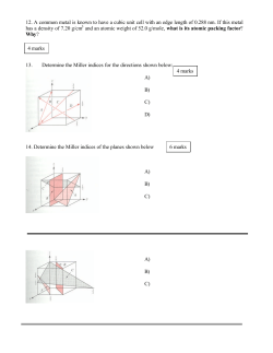


© Copyright 2026