
thesis. - CMT
﴾﴿
First-Principles Characterization and
Functionalization of Graphene-Like Materials
Ab initio karakterisatie en functionalisatie
van grafeenachtige materialen
Faculteit Wetenschappen
Departement Fysica
﴾﴿
First-Principles Characterization and
Functionalization of Graphene-Like Materials
Ab initio karakterisatie en functionalisatie
van grafeenachtige materialen
Proefschrift voorgelegd tot het behalen
van de graad van doctor in de wetenschappen
aan de Universiteit Antwerpen te verdedigen door
Jozef Sivek
Promotor
Prof. dr. Bart Partoens
Doc. dr. Hasan S¸ahin
Antwerpen, 2015
Members of the PhD jury
Chairwoman
Prof. Sandra Van Aert, University of Antwerp
Supervisors
Prof. dr. Bart Partoens, University of Antwerp
Doc. dr. Hasan S
¸ ahin, University of Antwerp
Members
Prof. Etienne Goovaerts, University of Antwerp
Prof. Luc Henrard, University of Namur
Prof. Michel Houssa, KU Leuven
Prof. Dirk Lamoen, University of Antwerp
Contact information
Jozef Sivek
http://www.uantwerpen.be/cmt
Jozef Sivek, 2015
Except where otherwise noted1 , this thesis is licensed under the Creative Commons
Attribution-ShareAlike 4.0 International License. To view a copy of this license,
visit http://creativecommons.org/licenses/by-sa/4.0/. Creative Commons
and the double C in a circle are registered trademarks of Creative Commons in the
United States and other countries. Third party marks and brands are the property
of their respective holders.
Electronic version2 of this document (with source and additional content) can
be obtained at address: http://cmt.uantwerpen.be/jsivek/thesis/
Cover image: see Fig. 6.2.3(b)
1
2
exception includes text (including equations and tables) of the chapters 4 to 8
this particular version, from May 8, 2015, as well as any other corrected versions
Contents
List of abbreviations
9
Preface
11
Acknowledgements
12
I
15
Introduction
1 2D crystals and precursors
1.1 Layered bulk materials . . . . . . . . . .
1.1.1 Graphite . . . . . . . . . . . . . .
1.1.2 Transition metal dichalcogenides
1.1.3 Group III-V compounds . . . . .
1.2 Two dimensional nanosheets . . . . . . .
1.2.1 Retrieval of the nanosheets . . . .
1.2.2 Graphene . . . . . . . . . . . . .
1.2.3 Silicene . . . . . . . . . . . . . .
1.2.4 Transition metal dichalcogenides
II
.
.
.
.
.
.
.
.
.
.
.
.
.
.
.
.
.
.
.
.
.
.
.
.
.
.
.
.
.
.
.
.
.
.
.
.
.
.
.
.
.
.
.
.
.
.
.
.
.
.
.
.
.
.
.
.
.
.
.
.
.
.
.
.
.
.
.
.
.
.
.
.
.
.
.
.
.
.
.
.
.
.
.
.
.
.
.
.
.
.
.
.
.
.
.
.
.
.
.
.
.
.
.
.
.
.
.
.
Methodology
17
17
18
20
21
22
23
27
28
30
33
2 Brief introduction to DFT
2.1 DFT scheme . . . . . . . . . . . . .
2.1.1 Schr¨odinger equation . . . .
2.1.2 Hohenberg-Kohn theorems .
2.1.3 Energy functional . . . . . .
2.1.4 Kohn-Sham approach . . . .
2.2 DFT to DFA . . . . . . . . . . . .
2.2.1 Basis sets and Bloch states .
2.2.2 Pseudopotentials and PAW
5
.
.
.
.
.
.
.
.
.
.
.
.
.
.
.
.
.
.
.
.
.
.
.
.
.
.
.
.
.
.
.
.
.
.
.
.
.
.
.
.
.
.
.
.
.
.
.
.
.
.
.
.
.
.
.
.
.
.
.
.
.
.
.
.
.
.
.
.
.
.
.
.
.
.
.
.
.
.
.
.
.
.
.
.
.
.
.
.
.
.
.
.
.
.
.
.
.
.
.
.
.
.
.
.
.
.
.
.
.
.
.
.
.
.
.
.
.
.
.
.
35
36
36
37
37
38
41
41
43
2.2.3
Exchange correlation functional . . . . . . . . . . . . . 43
3 Charge transfer methods
3.1 Bader charge analysis . . .
3.2 Voronoi charge analysis . .
3.3 Hirshfeld method . . . . .
3.4 Iterative Hirshfeld method
3.5 Modified Hirshfeld method
III
.
.
.
.
.
.
.
.
.
.
.
.
.
.
.
.
.
.
.
.
.
.
.
.
.
.
.
.
.
.
.
.
.
.
.
.
.
.
.
.
.
.
.
.
.
.
.
.
.
.
.
.
.
.
.
.
.
.
.
.
.
.
.
.
.
.
.
.
.
.
.
.
.
.
.
.
.
.
.
.
.
.
.
.
.
.
.
.
.
.
.
.
.
.
.
.
.
.
.
.
Results
45
46
47
47
49
50
53
4 Bilayer fluorographene
4.1 Calculation details . . . . . . . . . . . . .
4.2 Results . . . . . . . . . . . . . . . . . . . .
4.2.1 Fluorination of bilayer graphene . .
4.2.2 Properties of bilayer fluorographene
4.3 Conclusions . . . . . . . . . . . . . . . . .
.
.
.
.
.
.
.
.
.
.
.
.
.
.
.
.
.
.
.
.
.
.
.
.
.
.
.
.
.
.
.
.
.
.
.
.
.
.
.
.
55
56
57
57
62
67
5 Adsorption of Ti and TiO2 on graphene
5.1 Calculations . . . . . . . . . . . . . . . . . . . . .
5.2 Results and discussion . . . . . . . . . . . . . . .
5.2.1 Properties of Ti monolayer on graphene . .
5.2.2 Properties of TiO2 monolayer on graphene
5.3 Conclusions . . . . . . . . . . . . . . . . . . . . .
.
.
.
.
.
.
.
.
.
.
.
.
.
.
.
.
.
.
.
.
.
.
.
.
.
.
.
.
.
.
.
.
.
.
.
69
70
70
70
75
77
6 Atom decoration of silicene
6.1 Computational details . . .
6.2 Results . . . . . . . . . . . .
6.2.1 Atomic structure and
6.2.2 Electronic structure .
6.2.3 Stability analysis . .
6.3 Conclusions . . . . . . . . .
.
.
.
.
.
.
.
.
.
.
.
.
.
.
.
.
.
.
.
.
.
.
.
.
.
.
.
.
.
.
.
.
.
.
.
.
.
.
.
.
.
.
79
80
81
81
85
88
92
.
.
.
.
.
.
.
.
.
.
.
.
.
.
.
. . . . . . . . . . .
. . . . . . . . . . .
migration barriers
. . . . . . . . . . .
. . . . . . . . . . .
. . . . . . . . . . .
.
.
.
.
.
.
7 Stone-Wales defects in silicene
95
7.1 Computational details . . . . . . . . . . . . . . . . . . . . . . 96
7.2 Results . . . . . . . . . . . . . . . . . . . . . . . . . . . . . . . 97
7.2.1 Formation and stability of Stone-Wales defects in silicene 97
7.2.2 N-doped silicene: effect of Stone-Wales defects . . . . . 100
7.3 Conclusions . . . . . . . . . . . . . . . . . . . . . . . . . . . . 105
8 Inducing giant magnetic anisotropy
8.1 Computational details . . . . . . . . . .
8.2 Results . . . . . . . . . . . . . . . . . . .
8.2.1 Structural and stability properties
8.2.2 Magnetic properties . . . . . . . .
8.3 Conclusions . . . . . . . . . . . . . . . .
IV
Summary
.
.
.
.
.
.
.
.
.
.
.
.
.
.
.
.
.
.
.
.
.
.
.
.
.
.
.
.
.
.
.
.
.
.
.
.
.
.
.
.
.
.
.
.
.
.
.
.
.
.
.
.
.
.
.
107
. 108
. 109
. 109
. 110
. 118
119
9 Summary
121
9.1 Outlook . . . . . . . . . . . . . . . . . . . . . . . . . . . . . . 122
10 Samenvatting
125
A Bloch states
127
Bibliography
129
List of publications
153
Software
153
7
8
List of abbreviations
Γ A usual Bouckaert-Smoluchowski-Wigner notation [1] used for labelling
zero vector in reciprocal space, it is one of many commonly used letters
(M, K, ..) for specific high symmetry points of first Bruilin zone
2D Two dimensional
3D Three dimensional
˚
A ˚
Angstr¨om, unit of length equal to 10−10 m
AIM Atoms in molecules
BZ Brillouin zone
CMOS Complementary metal–oxide–semiconductor technology for constructing integrated circuits
CVD Chemical vapour deposition
DFA Density functional approximation [2]
DFT Density functional theory
DFT+U DFT with Hubbard-corrected energy functionals with explicit on
site Coulomb interaction correction terms [3]
DOS Density of states
FG Fluorographene, also known as graphene fluoride, a fully fluorinated
graphene with stoichiometry CF and sometimes referred as monolayer
in the text
GGA Generalized gradient approximation
GW It refers to GW approximation used to calculate the self-energy of a
many-body system of electrons, G stands for Green’s function and W
for screened Coulomb interaction
9
Hirshfeld-I Iterative Hirshfeld charge population analysis (see Section 3.4)
HOMO Highest occupied molecular orbital
LDA Local density approximation
LUMO Lowest unoccupied molecular orbital
MAE Magnetocrystalline anisotropy energy [4]
MD Molecular dynamics
MX2 Transition metal dichalcogenide general chemical formula, M stands
for the metal and X for chalcogen atom
NVE Microcanonical (ensemble), where number of particles in the system (N), the system’s volume (V) and the total energy in the system (E)
are kept fixed
PAW Projector augmented waves
PBE Perdew, Burke, and Ernzerhof [5] GGA parametrization
SW Stone-Wales (defect)
TM Transition metal
TMDs Transition metal dichalcogenides
VASP Vienna Ab-initio Simulation Package
Indication symbol for an image (its equivalent or part) that is available at Wikimedia Commons
10
Preface
Graphene has become the most prominent member and public face of the
new wave of research which essentially started after successful isolation of
stable monolayer materials in 2004.[6, 7] More than ten years after the first
excitement about the ”impossible” material graphene, the scientific research
bloomed into a large volume of multiple, experimentally observed, ultra-thin
materials with even a larger set of unique characteristics. Exploration of the
other quasi two-dimensional materials evolved almost parallel with the efforts
to bend and shape the electronic and surface properties of graphene via its
chemical and mechanical functionalization. These new materials proved to
be essential for reaching future goals of superstructures of ultra-thin crystals
with tailored applications. Not surprisingly, a large volume of these materials
share the hexagonal lattice structure and electronic similarities with graphene
and are, in that sense, named graphene-like materials.
The aim of this thesis is to explore the characteristics of a wide group
of graphene-like materials. First-principles methods are applied as the main
tool for describing as well as engineering of the particular properties via
chemical patterning. The extension of the set of studied pristine materials in
this thesis evolved as a natural response to the experimental progress in this
field, our available scientific methods and the possible industrial applications.
This work mainly focuses on chemical decoration of graphene-like crystals with chemical elements mainly in their single atomic form. This allows
mutual comparison and a much more selective approach to tailoring the properties of the derived materials. The following thesis is divided into three main
parts. The first one introduces the pristine materials and their precursors
in chapter 1, an essential building block of further study. The second part,
in Chapters 2 and 3, provides an overview of the applied methods. Finally,
the results are grouped in the third part, in Chapters 4 to 8. The results
part begins with the investigation of bilayer fluorographene (4), which is a
graphene derivative with modified electronic and chemical characteristics.
Next, in chapter 5, the patterning of pristine graphene with titanium and its
oxide, is discussed. Following two Chapters 6 and 7 contain results about
11
patterned silicene, a later discovered monolayer of silicon, its chemical reactivity and the influence of Stone-Wales defects on its chemical and electronic
properties. This part ends with Chapter 8, which discusses a directed decoration of fluorographene and molybdenum disulfide with the aim to engineer
the intriguing magnetocrystalline anisotropy properties. Finally a summary
with the conclusions is given in Chapter 9.
12
Acknowledgements
Today it seems so clear how the circumstances have evolved into the events.
Yet it is unclear how actions and thoughts of people affected one’s flow.
You read these lines from pure curiosity or from utmost hope to find Your
name among the ones which are given an acknowledgement or credit. If the
later is the reason of Yours reading, then know, that I express You a true
gratefulness, which should never be shown less than by my deeds and more
than by an unbreakable commitment.
Despite the idle nature of these words, which should be normally spared
for more clear reports, it is appropriate to name the indispensable groups.
Those who brought me here, now and in the form of myself. Therefore
the siblings, parents, beloved ones, good friends as well as rivals, relatives,
masters, peers, colleagues and unknowns are written in these words.
In addition to that, thanks are granted to an institution which allowed
this work, folks which supported it is and free software movement which
made it possible.
13
14
Part I
Introduction
15
Chapter 1
2D crystals and precursors
The existence and history of 2D crystals is tightly connected with layered
bulk materials. Compounds with the intriguing layered structure, including
clays, chalcogenides, hydroxides, silicate minerals as well as graphite and
hexagonal boron nitride, attract already for a long time the interest of the
scientific research community. The research spread across multiple scientific
disciplines and industrial applications, from engineering of industrial materials to condensed matter theory.
To properly talk about 2D materials one should inevitably discuss layered
materials in the first place, because those are the well recognized precursors
to the ultrathin structures. Afterwards the monolayer crystals which are
essential for the aims of this thesis will be described to provide a firm and
broader base ground for the results.
1.1
Layered bulk materials
Layered materials form a large and important group of the naturally occurring compounds. The aforementioned clays and ceramics found their use in
civil engineering, materials engineering as well as in high-temperature superconductivity. The chalcogenides became an essential part of the semiconductor industry and mechanical engineering applications. Materials like graphite
and hexagonal boron nitride have reached wide utilization from metallurgy,
through artistic media, up to the medicine.
The common and defining feature of these layered materials is their underlying crystal structure of coupled, ultra thin layers. This form determines
their mechanical properties as the self-lubrication in the case of graphite or
hexagonal boron nitride,[8, 9] but as well their electronic features promoting
the effects of quantum confinement. The list of layered materials includes
17
18
CHAPTER 1. 2D CRYSTALS AND PRECURSORS
graphite, transition metal dichalcogenides, layered clays and even MoO3 ,
GaTe, or Bi2 Se3 with diverse electrical, mechanical and optical properties.[10]
In the following Sections we discuss only a few of the bulk crystal precursors, consisting of weakly coupled (van der Waals-like interaction) layers
with strong in-plane bonding.
1.1.1
Graphite
Graphite, a crystal composed purely out of carbon atoms, is the most abundant carbon allotrope in nature. It belongs to the class of graphitic materials
with sp2 hybridized C atoms (see inset c–e of Fig. 1.1.1), unlike diamond
with sp3 hybridization (see inset a and b in Fig. 1.1.1).
a)
b)
e)
c)
d)
C
Figure 1.1.1: Few of the many carbon allotropes. a) Diamond, entirely composed of sp3 hybridized carbon atoms, b) amorphous carbon which is a polycrystal
of graphite and diamond, and it is linked together by an amorphous carbon network. Lower row displays graphitic (derived from graphite) carbon allotropes—sp2
bonded materials: c) zero dimensional fullerene, a C60 bucky-ball, d) one dimensional single walled carbon nanotube and e) graphite, the 3 dimensional material
composed of two dimensional graphene sheets.
Graphite has a layered crystal structure. Each layer is composed of sp2
hybridized carbon atoms ordered in a perfectly flat honeycomb lattice with an
interatomic distance of 1.42 ˚
A.[11] The weak bonding between the individual
sheets, separated at a distance of around 3.35 ˚
A, is carried by the van der
Waals forces. It is the underlying crystal form that allows the mechanical
1.1. LAYERED BULK MATERIALS
19
exfoliation at the macroscopic scale. As can be seen in Fig. 1.1.2 three
possible stackings exist. The Bernal AB stacking of the layers is the most
energetically favourable as well as abundant form (80 % [12]) compared to
simple hexagonal AA (normally not observable in crystalline graphite [13])
or rhombohedral ABC stacking (second most abundant).
a)
b)
ABC
c)
AB
d)
C
AA
Figure 1.1.2: a) Balls and sticks model of AB stacked graphite with highlighted
the unit cell composed of 4 atoms. The right panel displays a schematic top view
of the structure with various layer stackings: b) ABC stacking, c) most stable AB
stacked graphite and d) AA stacking.[14]
Graphite is an electric conductor, more specifically it is a material with
semimetallic behaviour with low density of states around the Fermi level
and a band overlap of about 41 meV (AB stacked form).[15] Its electronic
structure is dominated by the in-plane interactions, however the small band
overlap is a direct result of the interlayer interactions, with slight variations
among the different allotropic structures [11]. Without the interlayer interactions (the 2D situation) the density of states at the Fermi level decreases
to zero. The conductance is a result of delocalized π electrons within the
carbon layers, and thus it has an anisotropic character.
Due to graphite’s electronic and mechanical properties its use is limited
to the more conventional industrial applications, for example as electrical
conductor in arc electrodes, carbon brushes in commutators or in battery
anode constructions or as a dry lubricant for general industrial use.
20
CHAPTER 1. 2D CRYSTALS AND PRECURSORS
1.1.2
Transition metal dichalcogenides
Transition metal dichalcogenides (TMDs) belong to the wider group of compounds, the chalcogenides. The chalcogenides, as the name implies, are materials composed of chalcogen atoms, group VI elements1 , together with an
element with lower electronegativity. The specific group of interest is the
semiconducting transition metal dichalcogenides, with sixfold coordination
bonding of the transition elements with chalcogenides in the prismatic form
with general chemical formula MX2 . These TMDs form layered crystal structures.
The individual layers contain strong metal-chalcogenide covalent bonds
and the interlayer bonding is provided by the weaker van der Waals’ like
interaction between chalcogenide atoms. The two alternating layers with
hexagonally closed-pack chalcogenide atoms create the so called 2H structure2 (see molybdenum disulfide in Fig. 1.1.3) with two alternating layers
with trigonal prismatic coordination.[16] Multiple polytypes do exist, the
cubic close-packed with rhombohedral symmetry, or the 3R structure, with
three distinctive layers with trigonal prismatic coordination of chalcogenide
atoms, etc.[17] The possible stackings are similar to the graphite stacking we
have mentioned earlier.[18]
Examples of the TMDs with the aforementioned crystal structure include
molybdenum disulfide (MoS2 ), molybdenum diselenide (MoSe2 ), tungsten
disulfide (WS2 ), tungsten diselenide (WSe2 ) and molybdenum ditelluride
(MoTe2 ). It is worth noting that the alternative CdI2 -like (see 1T structure
in Fig. 1.2.6) semimetal structures do exist with similar stackings, however
with the octahedral structure of the sixfold coordination bonding of the transition elements with ligands. Examples are titanium disulfide, diselenide or
ditelluride (TiS2 , TiSe2 or TiTe2 ).[19, 20]
Due to the layered structure, the TMDs do share similar mechanical
properties with graphite and hexagonal boron nitride, and are utilized in
e.g. industrial surface protection.[21]. The same mechanical properties enable the mechanical exfoliation of the two dimensional crystals from their
bulk counterparts.[22] However, there exist semiconducting MX2 compounds
unlike semimetal graphite.[23] Therefore the investigation of their monolayers is noteworthy and provides a route to an electronically different class of
ultrathin materials.
1
Although oxygen belongs to group VI, usually only sulfur, selenium and tellurium
atoms are considered because of very different chemical behaviour of oxygen compared to
the other elements.
2
2H stands for two layers in the unit cell with hexagonal symmetry.
1.1. LAYERED BULK MATERIALS
21
a)
b)
1/3
c)
S
Mo
1/3
Figure 1.1.3: Ground state structure of the bulk crystal of molybdenum disulfide
with hexagonally close-packed sulfur atoms in the alternating layers. In the inset
a) the prismatic distribution of the sulfur atoms is clearly visible (sulfur atoms
bonded to one Mo atom make up the corners of prism). The b) top and c) side
view of the unit cell, consisting of 2 molybdenum and 4 sulfur atoms, displays the
alignment.
1.1.3
Group III-V compounds
Chemical elements of group III and V are known to create binary compounds
with crystal structures similar to the previously discussed graphite and other
carbon allotropes. For a long time they are already present in the microelectronics and optoelectronics industry, though their importance increased
after the large attention that was given to two dimensional materials like
graphene.[24–29]
The variety of the crystalline forms of these compounds is comparable to
the carbon allotropes and include layered materials with hexagonal symmetry. The range of different compounds include non layered hexagonal wurtzite
structures (w-BN, GaN, AlN, α-SiC) with tetrahedrally coordinated atoms
like in hexagonal diamond, zincblende structures with atoms in tetrahedral
coordination like in the diamond cubic crystal (GaAs, β-BN or c-BN), cubic
rock salt structures (binary compounds from group III and VI elements) or
finally hexagonal layered crystals (α-BN or h-BN, AlN sheets [30]).
22
CHAPTER 1. 2D CRYSTALS AND PRECURSORS
One of the leading examples is the diatomic compound, boron nitride
(h-BN). It shares many mechanical and chemical properties with graphite.
The compounds h-BN, GaN, AlN, GaAs and AlAs are semiconductors with
applications in the semiconductor industry, manufacturing of optoelectronic
devices, or applications utilizing their mechanical and piezoelectric properties. However, in the context of layered materials and the derived 2D crystals
only h-BN [31] and AlN [32] remain promising.
1.2
Two dimensional nanosheets
The separation of layered solids into individual layers was questioned for
a long period of time. It was unclear whether it was even possible due
to concerns about their stability at finite temperatures [33, 34]. The long
lasting stand-off was broken in 2004, when the first successful isolation of
two-dimensional atomic crystals was reported by K. S. Novoselov, et al. [33]
Among the first isolated crystals were dichalcogenides, graphene, BN, NbSe2
as well as Bi2 Sr2 CaCu2 Ox . This experimental achievement ultimately made
a broad scientific community to focus at this new class of materials with one
leading prime member, graphene.
The first separation of 2D materials has been performed by exfoliation of
layered bulk materials. Thus graphene, boron nitride and molybdenum disulfide have been exfoliated from graphite, hexagonal boron nitride or molybdenite, respectively. The exfoliated sheets are not true two dimensional objects, rather quasi 2D materials with a macroscopic size in two principal
dimensions and a thickness of several atoms.
Thanks to the intriguing nature of ultrathin materials the effect of their
successful isolation was exceptionally broad. The dimension reduction in the
crystals elevate the effects of quantum confinement which could be directly
exploited [35] and their planar structure revealed unmatched mechanical [36]
and chemical features. Furthermore it seeded theoretical exploration, engineering and even synthesis of a whole class of materials: chemically functionalized materials, e.g. graphene based graphane, fluorographene, their
bilayer forms, graphene oxide, “graphene-like” materials such as silicene,
germanene,[37–39] stanene,[40] other two dimensional crystal candidates including hydroxides, metal oxides, graphyne,[41] borophene, single-layer black
phosphorus (phosphorene),[42] etc. Nowadays, also sandwich-like structures
of these different 2D materials are realized, which allows to tune the properties of these layered structures.[43, 44]
Further we will discuss a couple of notable examples of ultrathin materials which are relevant for our results discussed further in this thesis, includ-
1.2. TWO DIMENSIONAL NANOSHEETS
23
ing graphene, chemically modified graphene, silicene and transition metal
dichalcogenides. The focus lies on their common properties, synthesis and
structure.
1.2.1
Retrieval of the nanosheets
Important aspects of 2D materials can be captured by understanding the
conditions and methods used in the process of their synthesis or extraction.
Two major method classes exist. The first one includes the top–down procedures, commonly called exfoliation techniques, where the molecular thin
crystals are separated or grown from the bulk precursors. The second class of
bottom–up practices, represents actual synthesis methods from other chemical compounds.[45]
Exfoliation techniques
The exfoliation methods are the most direct way for obtaining 2D crystals.
The group of bulk materials for which the exfoliation technique can be efficiently used includes graphite, hexagonal boron nitride, transition metal
dichalcogenides and transition metal oxides. [22]
The mechanical exfoliation is the most direct approach of extraction of
single or multiple layers out of layered bulk crystals. The extraction employs
mechanical cleaving. The best known example is the mechanical exfoliation
of graphene with a technique called the ’scotch-tape method’. The process
itself consists of repeatedly peeling of highly oriented pyrolytic graphite (a
crystal of almost pure hexagonal graphite [11]) which is performed by repeated sticking of an adhesive tape. In this way the weak interlayer forces
can be overcome ending up with a single molecular layer from the layered
crystal.[33] 3
The direct advantages of the mechanical exfoliation are the simplicity of
the method, which can be employed within a couple of hours, and the quality
of the obtained samples, which is of high grade, hard to be matched by other
techniques.[46] However, the main disadvantage is the lack of scalability, in
terms of the sample size as well as the amount of time required for the
production. Moreover, the nature of the technique gives little control over
the number of exfoliated layers and the actual shape of the crystals.[47]
An alternative approach is the liquid assisted exfoliation. The bulk materials are exfoliated in a solvent with or without assistance of intercalation
compounds or mechanical acceleration such as sonication. The obtained
3
Exfoliated mono to few layer thick graphite films of the size up to 10 µm were extracted
and they were inspected optically after direct transfer on a Si/SiO2 substrate.[6]
24
CHAPTER 1. 2D CRYSTALS AND PRECURSORS
flakes of a few molecular layers are afterwards transferred to a substrate
by spraying, mechanical transfer or by drying the suspension. The variety of method implementations is large, especially because of the number
of layered materials and the specific processes (oxidation, intercalation or
exchange, treatment by solvents, etc.).[10]
Most of the TMDs are suitable for the liquid-phase exfoliation,[22] the
metallic layered compounds TaS2 and NbS2 can be exfoliated by intercalation of water , MoS2 can be exfoliated in an aqueous suspension, [48] graphite
flakes can be separated into individual layers by sonication in a dichlorobenzene solution, [49] etc. The discovery of the liquid exfoliation was an important advancement and it is a research field under constant development4 as
it allows production of large quantities of nanosheets.
Unlike the liquid exfoliation techniques chemical exfoliation realizes the
final 2D material through intermediate steps with chemically modified compounds which can be exfoliated much more easily in the solvents in the form
of a colloidal dispersion. The well known intermediate compound for the
production of graphene is graphene oxide. It is produced from graphite that
is oxidized with use of strong acids and oxidants, like in the Brodie, Staudenmaier and Hummers method.[50] After oxidation the individual graphene
layers are heavily disrupted with a large portion of carbon atoms creating
bonds with hydroxyl and epoxy groups. These sheets of layered material are
strongly hydrophilic, which makes it easy to intercalate water between the
layers and thus to create a colloidal suspension of graphene oxide in a water
or other polar solvent with the help of sonication.
The atomic structure of graphene oxide is still not fully understood. On
it own it can be used for production of various materials like thin layered
paper-like insulating films. However its reduced form is of most interest.
The reduction is performed with the assistance of chemical reductants, use
of ultraviolet light or with thermal-based methods. The resulting material
on the atomic level is disrupted graphene with defects and further treatment
to remove residual oxygen and to reconstruct pristine graphene is required
to reclaim its electrical conductivity.
Transition metal dichalcogenides like MoS2 , WS2 can be easily exfoliated via organolithium reduction chemistry. [51, 52] However these methods do suffer from low yields and poor quality of produced compounds (defects, structural and chemical changes).[53] Recently high yield methods of
chemically driven exfoliation techniques, usable for transition metal dichalco4
An example of constant development progress are the new promising solvents like
methyl-pyrrolidone suited for hexagonal boron nitride or isopropanol for TMDs. They
allow scalable processes with lower sensitivity to environmental conditions (like air or
water).[22]
1.2. TWO DIMENSIONAL NANOSHEETS
25
genides, were reported.[54] The process is similar to the previous attempts
albeit much more complicated. The intermediate compounds are made of
chalcogenides and lithium, potassium or sodium naphthalenide and in comparison to oxidation/reduction chemistry the process is suited for production
of high quality materials.[54]
Synthesis techniques
Synthesis techniques unlike exfoliation ones do not require bulk layered material as precursors. The bottom up approaches are known to be very suitable
for the large scale production of two dimensional crystals due to the scalability of the process and the reasonable to superior quality of the produced
samples.
Probably the most promising method for scalable and continual production is chemical vapour deposition (CVD). In the last decade large attention
was given especially to the CVD synthesis of graphene due to its attractive
electrical properties as a transparent conductive film, but TMDs, silicene and
other monolayers can be produced in a similar fashion.
The synthesis process of graphene consists of exposing a metallic foil (Cu,
Ni, Ru, etc.) in a high temperature reactor to the presence of organic compounds as a source of carbon atoms (CH4 , etc.) mixed in the gas atmosphere
(H2 , Ar, etc.). After the crystal synthesis the graphene layer can be transferred directly with the use of epoxy resin and polymers [55] or indirectly
by a transport film or etching the metal substrate. The known drawbacks
of this approach are the low control over the number of graphene layers as
well as the polycrystallinity of the material which depends on the polycrystallinity of the substrate metal. Despite shortcomings the method is very
attractive for the volume production of large scale transparent conducting
films with use in transparent and flexible electronics, materials protecting
films, chemical sensors, filters, etc. The possible applications are driving
continual improvements.[56]
Under the similar experimental conditions the growth of silicene is possible as well. The first experimental evidence of successful epitaxial growth was
reported by Padova et al. [57] followed later by the other experimental groups
which have realized and observed silicene sheets grown from evaporated Si
on a top of mainly Ag surface in ultra high vacuum.[58, 58–61]
The growth of molybdenum disulfide is much more sensitive to the environmental conditions, including highly crystalline metal substrates or vacuum requirements.[62] However, the successful CVD growth has been reported of the large area MoS2 and WS2 samples on amorphous SiO2 substrates [63] by sulfurization of deposited thin metal films.[64] In the process
26
CHAPTER 1. 2D CRYSTALS AND PRECURSORS
MoO3 (or WO3 ) and sulfur powder is heated to 650°C which allows the components to diffuse and form one to few layer crystals of chalcogenides on the
nearby placed pretreated substrate.
Alternative synthesis methods do exist, specifically for the production of
graphene and carbon based materials, with unique features not feasible with
exfoliation methods neither CVD methods. First of them is the epitaxial
growth of graphene, which can be performed with silicon carbide (SiC) by its
decomposition at high temperatures and creating few layer graphene on its
surface.
The 4H-SiC and 6H-SiC polytypes of semiconducting hexagonal SiC are
commonly used, with different stacking of the hexagonal Si-C bilayers.[12]
The (0001) surface of SiC is pretreated, to lower the roughness and to remove
the coating SiO layer. Afterwards it is annealed in noble gas atmosphere to
graphitization temperature (between 1000 and 1500 °C) to allow Si atoms
to sublimate and also to diffuse through the growing graphene film. The
epitaxial graphene (multi)layer is separated from the underlying surface by
the buffer layer and it can be lithographically patterned and contacted with
metal contacts.[65] The main advantage of epitaxial growth is the control over
the structural uniformity over large areas, because the crystal orientation of
graphene is coupled with the crystal structure of the substrate SiC wafers.5
Furthermore, this method is a viable candidate for all-carbon post CMOS
technology and graphene based electronics,[12] with the advantage of the
mass production, high crystal quality and reuse of contemporary silicon based
electronics processes. However, the process needs further improvements to
resolve sensitivity to the miscut of silicon carbide wafers.[66]
The second method is the chemical synthesis of carbon based macromolecules from polycyclic aromatic hydrocarbons, which is a field with long
history in chemistry. The route of a chemically driven, bottom–up approach,
may not be appealing for the synthesis of large two dimensional sheets of
structurally simple materials like graphene, however there is a large set of
more complex monolayer crystals without bulk counterparts including graphyne, its boron nitride analogue,[67] graphdiyne,[68] other planar benzenebased macromolecules, nanoribbons (1D structures),[69, 70] etc. which will
benefit from the advances in available methods from organic chemistry.
5
This requirements is especially important in connection to reproducible production
and possible graphene ribbon cutting.
1.2. TWO DIMENSIONAL NANOSHEETS
1.2.2
27
Graphene
Graphene is the first known member of the group IV elements 2D crystals
with a honeycomb like lattice which can exist in free standing form. The subtle reasons for its stability under the experimental conditions may be provided
by the corrugations of its surface with a lateral size of several nanometres
and out of plane deformations with heights up to 1 nm.[71]
a)
b)
A
C
B
Figure 1.2.1: a) Ball and sticks model of a single graphene sheet with highlighted
in-plane unit cell composed of two carbon atoms. b) Schematic top view on the
hexagonal honeycomb lattice with highlighted two sublattices commonly known
as A and B.
The crystal structure of graphene stems from the graphite structure (see
Fig. 1.1.2). Graphene as a single layer of graphite, or macromolecule of
aromatic hydrocarbon, is composed of carbon atoms arranged in the honeycomb lattice, with every atom possessing three bonds with its neighbours (see
Fig. 1.2.1). The reason for its planar structure is the sp2 orbital hybridization that induces three in-plane σ bonds, while the remaining electron in the
pz orbital accounts for π bonds and is responsible for the conducting, chemical as well as structural properties.[72] The crystal unit cell has an in-plane
lattice parameter of 2.46 ˚
A and includes two equivalent carbon atoms which
are usually assigned to the A or B sublattice (see Fig. 1.2.1). The A and B
sublattices are two overlapping triangular lattices.
As can be seen from Fig. 1.2.2 graphene can be characterized as a semimetal (or alternatively as a zero band gap semiconductor) with vanishing
density of states at the Fermi level. The valence and conduction bands meet
together at two independent K and K’ points in the first Brillouin zone of
the reciprocal space (see Fig. 1.2.3). The energy dispersion at the K points
is linear (i.e. the energy is a linear function of the crystal momentum wave
vector measured relative to K point) very much like the energy dispersion of
massless fermion particles following the Dirac (Dirac-Weyl) equation. The
energy dispersion around the Fermi level has the form of E = ~kvf , with
28
CHAPTER 1. 2D CRYSTALS AND PRECURSORS
Graphene (GGA PBE)
Energy (eV)
2
0
-2
-4
-6
Γ
M
K
Γ
Figure 1.2.2: Electronic band structure and corresponding density of states
of graphene (EF = 0). Note the vanishing density of states at the Fermi level
where conduction and valence band touches at the K point (one can identify two
independent K and K’ points in the Brillouin zone where the band crossing occurs).
vf the Fermi velocity approximately equal to c/300.[12]. Because of the two
dimensional nature of graphene crystal, this electronic spectrum can be also,
to a great extent, described by the tight-binding model.[45, 73]
Exactly this Dirac spectrum, and related Dirac cones at K symmetric
points, are responsible for the large interest in the electronic properties of
graphene. The linear character of the energy dispersion theoretically leads
to effects such as universal ballistic conductivity, Klein tunnelling [74] and
the ambipolar electric field effect.[45] Although these results only apply to
the idealized perfect crystal of pristine graphene they provide us very much
needed insight into the experimentally observed properties.
However, the Dirac like electronic band structure of graphene is also a
major disadvantage for its use in most of the contemporary electronic applications which rely on the presence of a finite band gap. Thus a large
portion of the graphene based research is focusing on band gap engineering by applying electric fields,[75, 76] chemical functionalization (changing
sp2 to sp3 hybridization) of graphene,[77–79] mechanical functionalization
(nanoribbons),[80] etc. This handicap of graphene has even more motivated
the extensive exploration of other graphene-like and other two dimensional
materials.
1.2.3
Silicene
Curiosity and chemical similarity guided scientific research into designing
honeycomb structures out of the other group IV elements or of the combination of group III and V elements into binary compounds.[24] A promi-
1.2. TWO DIMENSIONAL NANOSHEETS
a)
29
b)
K
a1
a2
b1 Γ
b2
C
M
K'
Figure 1.2.3: a) Real space unit vectors and corresponding b) reciprocal space
vectors for graphene lattice (the first Brillouin zone is highlighted). Note the only
two dimensional reciprocal space which is effectively used even in the calculations
where the periodical unit cell has a finite size in the z direction. Also note that
all the compounds with a hexagonal lattice posses the same reciprocal lattice, this
includes silicene and TMDs which will be discussed further.
nent example of such a material is silicene, a monolayer structure of silicon. It has emerged as a few-atom-thick material with a potential to replace
graphene by its inherent compatibility with silicon based electronics. This
was underlined especially after its successful experimental observation and
synthesis.[57–60, 81] The reason for this claim is the fact its proven existence
opened a new path for a nanoscale material which might be easily functionalized (like graphene) and incorporated within electronics as we know it
today.[82]
δ
Si
Figure 1.2.4: Balls and sticks model of a single layer buckled hexagonal lattice
of silicene, the buckling is marked by buckling height δ. The in-plane unit cell
composed of two silicon atoms is highlighted.
Silicon atoms can create a single layer honeycomb lattice, with considerably larger interatomic distances compared to those of graphene, with a
lattice constant of 3.83 ˚
A.[83] Unlike graphene, with sp2 hybridized carbon
atoms and in-plane bonds, silicon atoms form due to their larger size and
30
CHAPTER 1. 2D CRYSTALS AND PRECURSORS
sp3 -like hybridization (neither sp2 nor sp3 ) a buckled hexagonal lattice with
buckling parameter (δ) of 0.44 ˚
A (see Fig. 1.2.4).[37] The buckling is a feature
shared among more hexagonal crystals made of group III, IV and V atoms
where the planar form cannot be stabilized with π bonds due to the large
interatomic distance. Only the first row element based compounds including
SiC, GeC, AlN, GaN, BN, graphene and their mixed compounds form planar
sp2 -only bonds.[24]
Silicene (GGA PBE)
Energy (eV)
2
0
-2
-4
Γ
M
K
Γ
Figure 1.2.5: The electronic band structure of free standing silicene with the
corresponding density of states (EF = 0). The vanishing density of states at the K
symmetry point resembles the band crossing in graphene, however first principles
calculations reveal that the significant spin-orbit interaction in silicene leads to a
small band gap of 1.47 meV, almost two orders of magnitude more compared to
graphene.
As was reported by early theoretical works, silicene is a semimetal with
linearly crossing electronic bands with vanishing density of states at the Fermi
level in a very similar way as we have observed earlier for graphene.[24, 37, 84]
The character of the band dispersion implies similar properties including
electrons propagating through the monolayer crystal structure of silicene as
massless fermions in the vicinity of the Dirac point. Additionally, some
unique features of monolayer silicene such as quantum spin Hall effect,[85] a
large spin-orbit interaction,[86] a mechanically tunable bandgap [87] and a
valley-polarized metallic phase [88] have been reported by theoretically based
studies.
1.2.4
Transition metal dichalcogenides
The last group of two dimensional materials, which we will describe in more
detail are the transition metal dichalcogenides.
1.2. TWO DIMENSIONAL NANOSHEETS
a)
31
c)
1H
S
S
Mo
Mo
b)
d)
1T
Figure 1.2.6: The insets a) and b) show two examples of crystal phases of
monolayer molybdenum disulfide. The c) and d) inset shows a schematic top view
on the 1H and 1T phase of MoS2 , respectively. The 1H ground state structure
has prismatic coordination of sulfur atoms around the transition metal atom and
the upper layer lattices of the chalcogenide atoms match with the lower one. The
metastable 1T phase shows octahedral coordination of the metal bonds with the
upper layer of sulfur atoms rotated by 30◦ with respect to the lower ones.
Unlike the previous one-atom thick hexagonal two dimensional materials, a monolayer of TMDs is formed consisting of three atomic levels: the
triangular lattice of transition metal atoms is sandwiched between an upper
and lower equilateral triangular lattice formed of chalcogenide atoms. The
ground state of the single layer crystal has prismatic coordination, where
the upper and lower layer sublattices of the chalcogenide atoms match. This
configuration is commonly known as the 1H phase (one layer with hexagonal
symmetry). However, a metastable 1T phase (one layer with tetragonal symmetry) does exist.[17] The 1T phase incorporates octahedral coordination of
the metal bonds with the ligands and the upper and lower layers of chalcogenide atoms are mutually rotated by 30◦ as can be seen in the inset d) of
Fig. 1.2.6. In addition also other non trivial structures were reported.[51, 89]
Depending on the composition, crystal structure or polytype, the TMDs
exhibit semiconducting or metallic properties.[17, 90] As an example, trans-
32
CHAPTER 1. 2D CRYSTALS AND PRECURSORS
MoS2 (GGA PBE)
Energy (eV)
2
0
-2
-4
-6
Γ
M
K
Γ
Figure 1.2.7: Electronic band structure and corresponding density of states of
a semiconducting monolayer of MoS2 in its most stable 1H phase (EF = 0). The
direct band gap at the K symmetry point is a feature of the monolayer MoS2 , in
the bulk form the indirect band gap appears between valence Γ point and a point
between Γ and K in conduction the band.[17]
formation of MoS2 from a semiconducting material phase to a metal material
phase occur with a change from the 1H to 1T structure. Additionally the
band gap in TMDs bilayers is tunable, like in graphene, under applied external field.[91]
Several TMDs such as MoS2 , MoSe2 , WS2 and WSe2 have large bandgaps
that exhibit an indirect to direct band gap transition from their bulk to monolayer form. For example the indirect band gap of 1.3 eV of MoS2 expands to
direct gap of 1.8 eV (see Fig. 1.2.7) in its monolayer form.[92] This indirect to
a direct band gap transition enables photoluminescence of monolayer MoS2
and is of importance for possible photoelectronic applications.[17, 92, 93]
Part II
Methodology
33
Chapter 2
Brief introduction to DFT
The density functional theory (DFT) formalism is probably the most spread
ab initio quantum mechanical modelling tool in the contemporary solid state
matter research. In this Chapter a short introduction and schematic overview
of its principles is presented, as it is the method of choice for the results
presented later in the manuscript.
DFT is build upon the premise that the properties of many electron systems, such as solid state crystals, molecules and matter in general can be expressed as functionals1 of the electron density, a single, scalar function. The
history of the formalism dates back to 1964 when the two Hohenberg and
Kohn theorems were formulated. They express the equivalence between the
electronic density and the all-electron wave function of a quantum mechanical many-body system. Shortly after, in 1965 the practical implementation
by Kohn and Sham was introduced. However, only the later improvements of
exchange-correlation energy, pseudopotentials and projector augmented wave
method together with advances in the computational infrastructure allowed
for its widespread use.
It can be stated that DFT is loosely based on the Thomas-Fermi model,
utilizing only the electron density, which was developed separately from the
wave function formalism in 1927. However, even the extension of this model
with the Thomas–Fermi–Dirac exchange energy term did not solve the shortcomings. While the Thomas-Fermi model is an example of a simple, fast and
to some extent usable method, it largely fails in the fundamental aspects
(e.g. description of the atom electron shell structure or molecular bonding).
Nevertheless, the Thomas-Fermi model, the first model based on the electron
density, is important for fundamental and historical reasons.
Next we discuss the DFT fundamentals and approximations.
1
In this context functional maps a function space to a space of scalars.
35
36
CHAPTER 2. BRIEF INTRODUCTION TO DFT
2.1
DFT scheme
2.1.1
Schr¨
odinger equation
The non relativistic solution of a quantum mechanical many electron system
can be fully described by the Schr¨odinger equation. If the Hamiltonian is not
an explicit function of time we can restrict ourselves to the stationary states,
for which observable properties remain unchanged. The stationary states are
defined by:
2
−~
ˆ
ˆ
∆+V Ψ
(2.1.1)
EΨ = HΨ =
2me
ˆ
with E the energy (further referred also as total energy of the system Etot ), H
ˆ
the Hamiltonian operator, V the potential (operator) and Ψ the all electron
particle wave function.
ˆ from Equation 2.1.1 can be written for
The Hamiltonian operator H
a system of N electrons (all electrons in all atoms) and M atomic nuclei
(crystals, molecules, etc.) as:
N
M
2 X
X ~2
ˆ =− ~
H
∆i −
∆α
2me i
2M
α
}
{z
} | α {z
|
Tˆn
Tˆe
−
N X
M
X
i
|
α
N
M
1
1X 1
1 X 1 Zα Zβ e2
Zα e2
e2
+
+
~ α| 2
~α − R
~ β|
4πε0 |~ri − R
4πε
r
r
2 α6=β 4πε0 |R
0 |~
i −~
j|
{z
} | i6=j {z
}|
{z
}
Vˆexternal
Vˆee
Vˆnn
with Tˆe the electron kinetic energy operator, Tˆn the nuclei kinetic energy operator, Vˆexternal the external potential created by nuclei acting on electrons,
Vˆee the electron-electron interaction operator and Vˆnn the nucleus-nucleus interaction operator. One can clearly see the major obstacle of this approach.
The size of the phase space (coordinates of all electrons, nuclei, spins and
more) rises linearly with the size of the system, beyond practical usability
with no analytical solution left for all but a few simple cases (e.g. the hydrogen atom).
A first approximation we will make is the Born-Oppenheimer approximation.
Born-Oppenheimer approximation
The Born-Oppenheimer approximation is also called the adiabatic approximation due to its resemblance to the adiabatic theorem. The slowly acting
2.1. DFT SCHEME
37
external conditions are the positions of the nuclei, which appear fixed due to
the large difference of the electron and proton (cores) masses. Therefore we
can neglect the kinetic term of the nuclei (inversely proportional to the mass
of the particles): Tˆn = 0 and we can consider the nucleus-nucleus interaction
to be effectively constant: Vˆnn ≈ constant. Within this approximation the
Hamiltonian becomes:
ˆ = Tˆe + Vˆexternal + Vˆee + Vˆnn
H
2.1.2
(2.1.2)
Hohenberg-Kohn theorems
The two fundamental theorems by Hohenberg-Kohn reveal the solution to
the unmanageable phase space size.
First Hohenberg-Kohn theorem
The first theorem states that the external potential in the Hamiltonian of
the system is a unique functional of the ground state electronic density of
the system, apart from a trivial additive constant.[94] In other words, the
observable physical properties of a many electron system are fully described
(via the functionals) by the scalar electron density function depending only
on 3 spatial coordinates.
The actual proof can be performed by means of reductio ad absurdum for
a non degenerate ground state2 . The postulate that two distinctive potentials
will lead to the same density leads to a contradiction, i.e. the inequality of
two identical energies.[45, 94]
Second Hohenberg-Kohn theorem
The second theorem states that the total energy of the system (E), expressed
as a functional of the electronic density, reaches its minimum for the ground
state electronic density.[94] In other words, the total energy of the system
with the external potential as the functional of the electronic density is minimized by the ground state density.
2.1.3
Energy functional
The Hohenberg-Kohn theorems allows one to find the ground state properties
of a system by minimizing the total energy expressed as functional of the
2
The restrictions on the non degenerate ground state was removed by the work of
Levy.[95]
38
CHAPTER 2. BRIEF INTRODUCTION TO DFT
electronic density. From the aforementioned Hamiltonian operator 2.1.2, we
can write the total energy Etot as:
Etot = EHK + Vnn [ρ]
with Vnn [ρ]3 a functional of the electronic density and the fixed positions of
the nuclei, and EHK (HK stands for Hohenberg-Kohn) equal to:
EHK = T [ρ] + Vee [ρ] +Vexternal [ρ] = FHK [ρ] + Vexternal [ρ]
{z
}
|
FHK [ρ]
with FHK [ρ] the universal functional4 and Vexternal [ρ] the potential energy
as function of vexternal , the potential of the atomic nuclei (the integration is
performed over the entire space Ω):
Z
Vexternal [ρ] = ρ(~r)vexternal (~r)d~r
Ω
where
M
X
1
Zα e
vexternal (~r) =
~ α|
4πε0 |~r − R
α
Hohenberg and Kohn proposed the form of the FHK [ρ] functional as the
sum of the dominant classical Coulomb and another GHK universal functional containing the kinetic energy terms and the corrections to the electronelectron interactions not present in following classical Coulomb functional
(VClassicCoulomb ):
ZZ
1
1 ρ(~r)ρ(~r 0 )
FHK [ρ] =
d~rd~r 0 +GHK [ρ]
2
4πε0 |~r − ~r 0 |
| Ω
{z
}
VClassicCoulomb
2.1.4
Kohn-Sham approach
The large contribution made by Kohn and Sham in 1965 was the expression
of the GHK functional. The Kohn and Sham approach obtains a solution via
an auxiliary system of noninteracting particles similar to the Hartree-Fock
method, however including exchange as well as correlation corrections.[96]
Vnn [ρ]Ψ = Vˆnn Ψ
If this functional would be known, the whole problem would be just a minimization
problem of the total energy as function of the electronic density. Unfortunately, we do not
know it.
3
4
2.1. DFT SCHEME
39
While it is trivial to express the kinetic energy, in the Hamiltonian of the
system, as a functional of the many-body wave function (see equation 2.1.1) it
is a difficult task to express the kinetic energy as a functional of the electronic
density. The idea of the Kohn-Sham approach is the use of an auxiliary
system of noninteracting electrons5 with the same electronic density ρ(~r) as
the original system of interacting particles. However, this second system
will experience a non-trivial effective potential composed of a well known
analytical part and complicated exchange and correlation corrections. Kohn
and Sham themselves suggested the local density approximation (more will
be explained later) of the exchange and correlation corrections which allowed
them to fully express the energy term. The proposed form of GHK is:
GKS = TS [ρ] + Exc [ρ]
with TS [ρ] the kinetic energy of an auxiliary system of noninteracting electrons and Exc [ρ] the exchange and correlation energy of a system of interacting electrons with density ρ(~r) (a small albeit very important correction).
We can trivially express Exc [ρ] as (see previous equations):
Exc [ρ] = (T [ρ] − TS [ρ]) + (Vee [ρ] − VClassicCoulomb [ρ])
Now we can write EHK as:
EHK = TS [ρ] + Vexternal [ρ] + VClassicCoulomb [ρ] + Exc [ρ]
In order to express the effective potential for an auxiliary system, we need
to create a link between the system of interacting and noninteracting electrons. The second Hohenberg-Kohn theorem allows us to write the stationary
equations for both systems as:
δES δEHK =
≡0
δρ ρ0
δρ ρ0
with ES [ρ] = TS [ρ] + VS [ρ] the energy functional for the auxiliary system.
Both energies EHK and ES reach their minimum at the same ground state
electronic density ρ0 (~r). VS [ρ] has the form:
VS [ρ] = Vexternal [ρ] + VClassicCoulomb [ρ] + Vxc [ρ]
with Vxc part of the effective potential expressed, with use of the stationary
property, as a function of the variation of the exchange correlation energy
5
A system of noninteracting electrons is solved by solving a one-particle Schr¨odinger
equation.
40
CHAPTER 2. BRIEF INTRODUCTION TO DFT
with respect to the electronic density:
Z
Z
δExc [ρ(~r)]
d~r
Vxc [ρ] = ρ(~r)vxc (ρ(~r))d~r = ρ(~r)
δρ(~r)
Ω
Ω
Now, with the effective VS [ρ] potential, we can write the Kohn-Sham (single particle Schr¨odinger) equations for an auxiliary system of noninteracting
electrons:
2
−~
ˆ
∆i + VS [ρ(~r)] ψi (~r) = εi ψi (~r)
2me
Kohn-Sham equations
N/2
2
X
X
2
|ψi (~r)|
ρ(~r) =
spin=1
i
(2.1.3)
with N the number of the electrons in the system. Note that in the definition
of the electronic density ρ(~r) we already assume the Pauli exclusion principle
for the electrons (fermions).
Kohn and Sham showed that with the use of the Hohenberg-Kohn theorems the equations for our problem of interacting electrons are identical to
the set of equations of noninteracting electrons in an effective potential VS .
Therefore, for a given VS , determined by the properties of our system, we can
search for the solutions of the Kohn-Sham equations and ultimately obtain
the ground state electronic density of the system as the sum of the first N 0
lowest energy solutions |ψi (~r)|2 and the ground state energy as:
0
E=
N
X
εi − VClassicCoulomb [ρ] + (Exc [ρ] − Vxc [ρ])
i
One needs to solve the Kohn-Sham equation self-consistently, because VS
depends on the actual electron density ρ. This is performed by constructing
an initial guess for the electron density, solving the equations, obtaining a new
density and energy (see above) and repeating this process until convergence
in both quantities is reached.
This procedure with a known analytical form of the exchange correlation
energy Exc provides an exact electronic ground state solution for a given
external potential of atomic cores. Additionally, one can find a ground state
structure (nuclear positions) with use of the Hellman-Feynman theorem [97].
The Hellman-Feynman theorem relates derivatives of the total energy
(like forces) to the expectation value of the derivative of the Hamiltonian:
Z
ˆ
dE
dH
=
ψ∗
ψdv
(2.1.4)
dλ
dλ
space
2.2. DFT TO DFA
41
The optimal configuration (if it exists) of the atomic cores can be found
by the following procedure. For an initial guess of the nuclear positions the
electronic self consistent loop is performed. Subsequently the forces acting on
the ions are calculated with the use of the Hellman-Feynman theorem. Next
the atomic cores are moved according to classical mechanics. The procedure
is repeated until the forces acting on the ions vanish.
2.2
DFT to DFA
We stated before that DFT is exact. Unfortunately in the real world implementation we are forced to use the density functional approximation (DFA).
In the following Sections we discuss the approximations made in the representation of the wave functions and exchange correlation energy. The use of
DFA is inevitable for any practical application due to numerical constraints
or missing knowledge.
2.2.1
Basis sets and Bloch states
It is convenient to express the wave functions as an expansion in a basis set.
There are two distinctive groups of basis sets, localized and nonlocalized.
For an isolated system without periodicity, the (atom) localized basis sets
(spherical harmonics, Gaussian functions, etc.) can be used. However many
systems are, or can be approximated as periodic crystals. The nonlocalized
basis set for the wave function representation is suited for periodic systems.
For periodic systems the Bloch theorem provides a natural way to express
the wave functions in a plane waves basis set of the single electron states
solution, as of the Kohn-Sham equations 2.1.3. The Bloch theorem and the
Bloch state describe a single electron moving in the lattice of ions. The wave
function of an electron in a periodic potential differs from the one of the
free electron by a modulation part (a function with the periodicity of the
lattice).[98]
The wave function of an electron in form of Bloch states is (for full explanation of the following form see Appendix A):
X
X
~
~
(2.2.1)
ψ(~r) =
C~k−K~ e−iK·~r eik·~r
~k∈1st BZ
~
∀K
|
{z
u~k (~
r)
}
where 1st BZ stands for the first Brillouin Zone, with ~k a reciprocal vector in
~ the reciprocal lattice point vectors. u~ (~r) is
this first Brillouin Zone and K
k
42
CHAPTER 2. BRIEF INTRODUCTION TO DFT
lattice periodic function. The used ~k for labelling the Bloch states directly
relates to the crystal momentum ~~k of an electron.
a)
b)
b1
b1
K
K
M
M
Γ
Γ
b2
b2
Figure 2.2.1: Example of Brillouin zone sampling of hexagonal lattice with a)
Γ centred and b) regular 6 × 6 × 1 Monkhorst-Pack grid, the first Brillouin zone
is highlighted as well as the irreducible Brillouin zone, which is the first Brillouin
zone reduced by all of the point symmetries of the lattice and is used to further
reduce numerical costs when applicable.
The Bloch states give us more than just an insight into the structure
of the solutions, they also provide a possible practical numerical solution.
Specifically it provides a recipe for the solution in the form of plane waves
~ in 2.2.1). The use of a plane wave basis set allows
(i.e. the summation over K
the use of fast Fourier transforms, does not depend on ion positions (as in
the case of localized basis sets like spherical harmonics, Gaussian functions)
and provides a systematic way of refinement.
The practical numerical limitations force us to clip the summation over
~
K vectors at a certain length of the vectors. This length is usually expressed
in the terms of a maximal energy, and it is named energy cutoff radius Ecut :
~ |K|
~ < Kcut ;
∀K,
Ecut =
~2 2
K
2me cut
This constraint results in a limited resolution in real space at the scale:
λ=
2π
Kcut
Similarly, the summation (integration) over ~k in the first Brillouin zone
in expression 2.2.1 can be approximated by the sum of well chosen points in
the first Brillouin zone. The most widely used set of points is build according
to the scheme of Monkhorst and Pack.[99] An example of such a set is shown
in Fig. 2.2.1.
2.2. DFT TO DFA
2.2.2
43
Pseudopotentials and PAW
In the previous Section we have outlined the use of a plane wave basis set.
However, the wave function typically seen in crystals requires a very large
basis set (Ecut ) due to the large wave function oscillations near the atomic
cores. To avoid this obstacle one needs to replace the actual wave function
with a smoother one. Because the problematic region lies in the vicinity of the
atomic nuclei, the core or inner shell electrons (which are usually dormant)
can be subtracted from the total wave function. The price for this approach
is the replacement of a simple Coulomb potential (vexternal ) created by the
nuclei with a much more complicated pseudopotential created by nuclei and
chosen number of core electrons.[100] The wave function with omitted core
electrons is called a pseudowavefunction, it describes the valence electrons
and is identical (due to the construction of the pseudopotential) to the full
electron wave function outside a chosen core radius.
The concept of pseudopotentials was further improved by Bl¨ochl who introduced the projector augmented wave (PAW) method.[101] It builds upon
the same premise of frozen core electrons which are removed from the calculation. Yet it provides a transparent way to reconstruct all electron wave
functions from the valence electron wave function, with the use of projector functions active in the chosen augmentation region close to the atomic
nuclei, and it properly describes the potentials from all-electron charge densities. Moreover, the use of the PAW method further increases the calculation
efficiency.
2.2.3
Exchange correlation functional
The missing ingredient to the Kohn-Sham equations 2.1.3 is the analytical
form of the Exc [ρ] functional. Kohn and Sham originally proposed in their
work [96] an exact form of the exchange correlation functional. We know it as
the local density approximation (LDA) of the Exc [ρ] functional. For the electronic density which is sufficiently slowly varying, the exchange-correlation
energy can be written in the form:
Z
LDA
Exc [ρ] = ρ(~r)exc (ρ(~r))d~r
Ω
with exc (ρ(~r)) the exchange and correlation energy per electron in a uniform electron gas with a density equal to ρ(~r), known from the theory of a
homogeneous electron gas.
The LDA works surprisingly well for a variety of crystals. The reason
for the usability of the LDA lies in the fair amount of error compensation
44
CHAPTER 2. BRIEF INTRODUCTION TO DFT
between the exchange and correlation parts of the functional. It is known
to slightly underestimate lattice parameters and to reasonably estimate the
medium to long range interactions (e.g. van der Waals interaction, hydrogen
bonds etc.) due to overestimation of the attractive potential.
Improvement over the LDA approach is the generalized gradient approximation (GGA). If LDA is the first term of the expansion of the exchange
and correlation energy in powers of the density gradient, then GGA includes
the next term of the series:[96]
Z
Z
GGA
Exc [ρ] = ρ(~r)exc (ρ(~r))d~r + |∇ρ(~r)|2 e(2)
r))d~r
xc (ρ(~
Ω
Ω
The improved form of the exchange and correlation energy with the corrections due to gradients in the electronic density is not without drawbacks.
GGA functionals are known to generally overcorrect LDA by overestimating the lattice parameters and additional medium to long range interaction
corrections are required (e.g. Van der Waals interaction).
The exc in both LDA and GGA has the form of the two additive parts,
representing contributions of exchange energy of electron and correlation
between electrons, with various possible representations:[2, 102]
exc (ρ(~r)) = ex (ρ(~r)) + ec (ρ(~r))
Chapter 3
Charge transfer methods
The motivation for the charge transfer calculation methods is to evaluate
charge transfer (and related physical variables as dipole moments) between
the individual atoms (or larger structures) in order to quantify some of the
observable properties of the molecules.
In the following we discuss possible methods to determine distribution
of charges in crystals. The main goal of all the approaches is to ascribe
the obtained multielectron charge density to individual atoms following the
concept of atoms in molecules (AIM).1 The AIM on itself is a construction
of the human mind, a tool, and on its own it is not directly observable by
experiment nor can be defined unambiguously.[103] The ambiguity originates
from the simple quantum mechanical fact that crystals are not just the sum
of their charged structural elements, e.g. atoms. This results in a multitude
of different techniques. Nevertheless, all these methods provide meaningful
and transparent approaches of electronic density division. Furthermore they
follow some obvious restrictions, like the computed charge transfer between
infinitely separated parts should be zero or that the symmetric compounds
exhibit symmetric charge transfers.
One of the early approaches to assign charge to the individual parts in
a compound was done by Mulliken.[104] The Mulliken charge population
analysis is one example of the many wave function based methods [105] and
the actual procedure came at no cost for methods using localized basis sets.
However, for DFT formalism methods based on nonlocalized basis sets, the
advantage disappears. Moreover, the transferability of the wave function
based methods is difficult if not impossible and the major drawback is the
large sensitivity to the choice of the basis function set. On the other side
there are the electronic density based methods with more intuitive as well
1
Atoms in molecules is a concept in which atoms and their bonds can be used to
express observable properties of molecular systems.
45
46
CHAPTER 3. CHARGE TRANSFER METHODS
as trustworthy appeal, benefiting from the that the electronic density is well
defined and easily obtained in the DFT formalism. In the following, several
charge density based methods are discussed.
3.1
Bader charge analysis
The Bader charge analysis was introduced by Richard F. W. Bader in 1990.[106]
The method is based on the partitioning of the real space into cells accommodating individual chemical atoms.
The space is divided by the surfaces of zero flux in the gradient of the
electronic density. This means the flux in the gradient vector field, of the all
electron density, vanishes at this zero flux surface.2 Mathematically we can
define the surface S(~r) as:
∇ρ(~r) · ~n(~r) = 0;
∀~r ∈ S(~r)
with ~n(~r) the normal to the surface S(~r).
The dominant feature of the all-electron density in the molecules and
crystals is that the density exhibits its maximum at the position of the nuclei.
This leads to the intuitive image of the partitioning scheme, where the space is
divided by the surfaces determined by the extremes (minima) of the electronic
density. In general3 the partitions contain a single nucleus and the charge
density enclosed in the separate spatial regions can be ascribed to individual
chemical atoms.
The usual form of the electronic charge density, obtained from the DFT
based software framework, is a grid sampled function in real space. Thus the
practical implementation of the Bader charge analysis is restricted to grid
based methods and generally cannot be solved analytically. The reconstruction of the zero flux surface and the subsequent integration, in the so called
Bader regions, had caused convergence problems and created additional numerical complexity.
Although the Bader method was first proposed in 1990 the first practical
application appeared only in 2006 by Graeme Henkelman et al.[107]. Instead
of finding the actual dividing surface, which is particularly difficult, they propose an algorithm which assigns each grid point (with corresponding charge)
to the one of the atomic regions by following a steepest ascent path on the
charge density grid. This allows robustness (independence on the compound
2
The idea for Bader charge analysis originates from the principle of least action where
the zero flux surface appear as one of the required conditions.
3
Sometimes regions without nucleus can occur, then they are assigned to the nearby
atom regions.
3.2. VORONOI CHARGE ANALYSIS
47
structure) and predictable scalability of the algorithm. The resulting Bader
charge is then just a sum over the charges at the grid points belonging to the
region defined by the common terminal point of the steepest ascent paths.
The aforementioned algorithm was further refined by Edward Sanville et
al. in 2007[108] and later by W. Tang et al. in 2009.[109] The improvements
included the correction of the grid bias (it causes a systematic deviation from
the true Bader surface if ascent trajectories are clipped to grid points) and
more accurate division of the charge at the Bader volumes boundary. The
improved procedure (with usable implementation available from Henkelman
Group at The University of Texas at Austin) also incorporates an iterative
approach to improve the speed of the algorithm when dealing with large
meshes.
3.2
Voronoi charge analysis
An appealing twist to the Bader partitioning scheme is the Voronoi charge
analysis method introduced by F. Matthias Bickelhaupt in 1996 [110] and improved to the Voronoi Deformation Density method by C´elia Fonseca Guerra
in 2003.[111] The principle is similar to the Bader charge analysis or other
minor partitioning schemes,[111] the space is divided to non-overlapping regions defined to be the Voronoi cells4 with the seeds the positions of the
nuclei.
The actual charge ascribed to the individual atom is the definitive integral
of the electronic charge density within the Voronoi cell of the particular
atom. The aforementioned improvement of C. F. Guerra was in the use of
deformation charge density (this term will be explained with the Hirshfeld
method) instead of the all-electon charge density, which results in the better
description of the charging effects due to the chemical bonding.
3.3
Hirshfeld method
The origin of the Hirshfeld charge analysis dates back to 1977 when it was
first proposed by F. L. Hirshfeld.[112] The main feature of this method is
that it assigns to each atom in the molecule its share of charge at each
space point of the charge density. There is neither a partitioning scheme
4
Voronoi cell or polyhedron is the set of points closest to the particular seed point,
the Voronoi cells are broadly presented in nature like honeycomb (from triangular seed
lattice), basalt stone columns or foam from soap bubbles.
48
CHAPTER 3. CHARGE TRANSFER METHODS
nor dividing surfaces like in the binary approaches where all charge density
located at some point is attributed to a specific atom or not.
The total charge density is divided into the atomic contributions:
ρ(~r) =
M
X
α
ρb.a.
r)
α (~
=
M
X
wα (~r)ρ(~r)
α
r) the atomic electronic density of bonded atom, M the number of
with ρb.a.
α (~
atoms and wα (~r) a sharing (weight) function according to which each point
in space is proportionally shared among all the atoms. The sharing function
is defined in respect to the isolated atom electronic charge densities:
wα (~r) =
(~r)
(~r)
ρatom
ρatom
α
α
=
PM atom
proto
ρ
(~r)
(~r)
β ρβ
with ρatom
(~r) the electronic density of free standing (isolated) atoms5 and
α
ρproto (~r) molecule (crystal) proto-density (or simply promolecule density) as
superposition of the free atom densities of the respective chemical atoms in
the compound. The sharing functions are all positive and by definition the
sum of all sharing functions is equal to one everywhere.
The core reasoning for such sharing function is the idea that the density
of the bonded system is comparable to the artificially created proto-density
composed of the free atomic densities. In the extreme case of the free atoms
(infinite separation) the aforementioned division of total density is just an
identity.
There are two strong points of the Hirshfeld approach compared to the
previous partitioning schemes. The first one is that the Hirshfeld method,
because of its construction, will show no charge transfer for the artificially
created system out of isolated atomic charge densities. The second one is the
choice of a stockholder recipe, i.e. charge at every point is divided between
all atoms, every atom has its own share, which according to Hirshfeld itself
is: ”A general and natural choice ... ”.
The density of the bonded atom is an overlapping continuously distributed
charge density assigned to the specific atom. It is convenient to define the
atomic deformation density from the density of bonded atom by ρb.a.
r) subα (~
tracting the electronic density of a free atom:
δρα (~r) = ρb.a.
r) − ρatom
(~r)
α (~
α
5
to be precise the full description will be: it is suitably positioned, spherically averaged
ground-state isolated atomic electronic density
3.4. ITERATIVE HIRSHFELD METHOD
49
or even molecular deformation density:
δρ(~r) = ρ(~r) − ρproto (~r)
which are useful for visualization purposes and determination of electrostatic
properties of the molecules.
By means of the Hirshfeld charge population analysis one can obtain the
total electronic charge of an atom by integrating the density of bonded atom
all over the space (Ω):
Z
ρb.a.
r)d~r
α (~
Qα =
Ω
The net atomic charge can be obtained by addition of nuclear charge or
alternatively can be expressed as definitive integral of the atomic deformation
density:
Z
δρb.a.
r)d~r
α (~
qα =
Ω
3.4
Iterative Hirshfeld method
On its own the Hirshfeld idea has very solid reasoning. However, it contains
one apparent arbitrary decision, it choose the neutral free atoms as a reference
systems. This choice leads to deficiencies especially in ionic systems.[113]
Patrick Bultinck et al. proposed in 2007 an important extension to the
original Hirshfeld scheme [113] and described its characteristics.[114] The
extension removed arbitrariness in the choice of promolecule and the known
shortcomings of the original approach, such as the small computed charges
in the comparison to the other methods or limitation of the method which
allowed only description of charge neutral systems.
The proposed algorithm is in essence the iterative refinement scheme for
the Hirshfeld charge population analysis. The first step is a regular Hirshfeld
method. From that we obtain the calculated valence charges on the bonded
atoms Qα . In the consecutive step we use the same approach but instead
of the (neutral) isolated atoms (for construction of the sharing function) we
make use of the (ionic) isolated atoms with valence charge equal to Qα from
the previous step. The iteration scheme is repeated until the convergence in
input and output valence charges is reached.
The sharing function becomes:
wα (i, ~r) =
ρatom
(i − 1, ~r)
α
;
ρproto (i − 1, ~r)
with ρatom
(0, ~r) ≡ ρatom
(~r) etc.
α
α
50
CHAPTER 3. CHARGE TRANSFER METHODS
and Qα (i) the calculated valence charge is used as a new valence charge on
isolated atom for the next step:
Z
Z
b.a.
Qα (i) = ρα (i, ~r)d~r = ρatom
(i + 1, ~r)d~r
α
Ω
Ω
with ρb.a.
r) = wα (i, ~r)ρ(~r). The process is repeated until the convergence
α (i, ~
in the charge population difference ∆α (i) between consecutive steps is sufficiently small.
∆α (i) = |Qα (i) − Qα (i − 1)|
The method itself does not require the initial atomic electronic densities
representing neutral atoms (the iterative nature will eliminate
initial arbitrary choice), albeit it is a common choice as the first step of
this iterative Hirshfeld (Hirshfeld-I) analysis returns the original Hirshfeld
populations.
The practical representation of the iterative Hirshfeld charge analysis has
been recently revived by Danny E. P. Vanpoucke et al., [115] with the focus
on the application of the method on periodic materials with the use of the
electronic density of fractionally charged isolated atoms constructed as the
linear interpolation between isolated atoms with integer charges.[116]
ρatom
(0, ~r)
α
3.5
Modified Hirshfeld method
In 2008 Ortwin Leenaerts introduced yet another modification of the Hirshfeld and iterative Hirshfeld methods named modified Hirshfeld and modified
Hirshfeld-I.[117] This method builds directly on the elements of the aforementioned approaches with small yet intriguing change. Instead of the atomic
charges he proposes the use of the molecular charges. This is a great simplification especially for large systems where the detailed charge redistribution is
of no aim and a full approach is an overcomplication. Probably the simplest
example which demonstrates the advantages of this approach is the adsorption of the molecules on the surfaces (e.g. two dimensional crystals). In these
systems the only required information is the charge relocation from/to the
adsorbent as a whole.
For the system composed of two distinct subsystems A and B the Hirshfeld weight function for the subsystem A will be:
P
atom
(~r)
α∈A ρα
P
; MA + MB = M
wA (~r) = P
atom
(~r) + γ∈B ρatom
(~r)
γ
β∈A ρβ
3.5. MODIFIED HIRSHFELD METHOD
51
The modified Hirshfeld will make use of a different weight function:
modif ied
wA
(~r) =
ρA (~r)
ρA (~r) + ρB (~r)
The practical implementation consists of the calculation of the total system electronic density and the subsequent calculation of the electronic density
of the subsystems in the same configuration as in the total system. These
densities can be afterwards used in the aforementioned modified Hirshfeld
method. If the charges are made self-consistent in this way, they will lead to
the modified Hirshfeld-I charges. This algorithm allows the total cost of the
numerical calculations to be lower compared to the atomic Hirshfeld methods
while maintaining most of the advantages of atomic based methods.[117]
52
CHAPTER 3. CHARGE TRANSFER METHODS
Part III
Results
53
Chapter 4
Bilayer fluorographene
In this Chapter1 fluorinated bilayer graphene, hereafter called bilayer fluorographene (for a better notion of the chemical composition and the structure, see Fig. 4.1.1), is investigated. The reason why the chemical derivative of graphene is studied is the fact that despite unique characteristics
of graphene,[75, 119–121] there exists a serious obstacle to use graphene in
electronics as we know it today. Graphene is a zero-gap semiconductor,
and the absence of a bandgap is protected by inversion and time-reversal
symmetry.[122] Among broad set of different approaches,[69, 78–80, 123–
128] the chemical modification, in which pz electrons are confined into covalent bonds and their hybridization is changed from sp2 to sp3 , was chosen.
An advantage of the chemical derivatives of graphene is the preservation
of the two-dimensional character of the material with vastly different electronic properties. Among the possible derivatives of graphene, there are two
that have attracted special attention, namely, graphane and fluorographene
(graphene fluoride), which result from the hydrogenation and fluorination of
graphene, respectively. They are theoretically predicted [129–136] and experimentally observed [79, 125, 126, 128, 137, 138] to form crystalline materials,
in contrast to, for example, graphene oxide. [139, 140]
As is apparent from the title of this Chapter, the process of chemical
modification is not restricted to monolayer graphene. It has been proposed
before that this process can be expanded to bilayer graphene as well. [141]
Ab initio calculations showed that the weak van der Waals forces between the
graphene layers are replaced by much stronger covalent bonds that stabilize
1
The results of this Chapter can be found in publication: J. Sivek, O. Leenaerts, B.
Partoens, and F. M. Peeters, J. Phys. Chem. C 116, 19240 (2012), ”First-principles investigation of bilayer fluorographene”.[118] Consult the rights and permissions for the text
of this Chapter (including equations and tables) with the publisher of the aforementioned
publication.
55
56
CHAPTER 4. BILAYER FLUOROGRAPHENE
the structure and that, at full coverage, a bilayer analogue of graphane is
formed. The electronic structure of intrinsic monolayer and bilayer graphane
are very similar,[142] but their mechanical/elastic properties are expected
to be substantially different. And the difference in elastomechanical qualities can be an important issue. It was recently demonstrated [143] that the
roughness of monolayer graphane surfaces is considerably larger than that of
graphene. This increase of the size of the ripple formation can be explained
by the lower stiffness of graphane [144] and its different vibrational properties
as compared with graphene. [145] One way to reduce the increased roughness
is to consider bilayers instead of single layers. As is well known from experiment, the ripple formation in bilayer graphene is strongly reduced; that is,
they are removed by the interlayer interaction.[146] A similar effect can be
expected for bilayer graphane where the interlayer interaction is even more
important.
Motivated by the previous theoretical and experimental work in this
Chapter it is investigated whether it is possible to fluorinate bilayer graphene
and to form bilayer fluorographene. Bilayer fluorographene, described further, is a much more stable compound than bilayer graphane, although
more fluorination is needed to induce interlayer covalent C–C bonds and
its 2D Young’s modulus is lowered to approximately 300 N m−1 compared
to graphene. The structure of this compound resembles those of monolayer
fluorographene and diamond.
Also a comparison is made to graphane, bilayer graphane, and fluorographene. Furthermore the effective masses around the Γ-point for fluorographene and bilayer fluorographene are found to be isotropic, in contrast to
earlier reports.
4.1
Calculation details
All our calculations were done within the density functional theory (DFT)
formalism as implemented in the VASP package [147] with usage of the local density approximation (LDA) and the Perdew, Burke, and Ernzerhof
[5] generalized gradient approximation (GGA) for the exchange-correlation
functional. We made use of the projector augmented wave method [101] and
a plane-wave basis set with an energy cutoff of 500 eV. The relaxation of
atomic positions was performed with forces smaller than 0.01 eV ˚
A−1 .
Three types of supercells were used: 3×3 and 2×2 supercells to study the
adsorption properties of fluorine on a graphene bilayer for different concentrations and configurations of fluorine and a 1 × 1 unit cell for the calculation
of the properties and electronic band structure of fully fluorinated graphene
4.2. RESULTS
57
and bilayer graphene.
The sampling of the Brillouin zone was done for the different supercells
with the equivalent of a 24 × 24 × 1 Monkhorst-Pack [99] k-point grid for
the monolayer or bilayer graphene unit cell (containing two carbon atoms
per layer). Spin polarization was not included in the calculations because
fluorination is not expected to induce magnetism in graphene. [148]
Because periodic boundary conditions were applied in all three dimensions, the height of the supercell was set to 20 ˚
A to include enough vacuum
to minimize the interaction between adjacent layers. Additionally, we have
performed a convergence test with respect to the planar size of the supercell.
We obtain an accuracy in binding energies of less than 0.1 eV and in bond
lengths of less than 0.01 ˚
A with the chosen 3 × 3 supercell.
Figure 4.1.1: Top and side view of bilayer fluorographene. The carbon atoms
of the two layers are given by different colours (shades) for clarity and the fluorine
atoms are in light green (light circles with the smallest diameter).
4.2
4.2.1
Results
Fluorination of bilayer graphene
The main objective of this paper is to investigate chemisorption of fluorine atoms on both sides of bilayer graphene. Hydrogenation and fluorination of the carbon atoms of graphene change their hybridization from sp2
to sp3 . In the case of hydrogenation of bilayer graphene, it was demonstrated that stable interlayer C–C bonds are induced at high concentrations of
58
CHAPTER 4. BILAYER FLUOROGRAPHENE
adsorbates.[141] In this Section, we perform a similar study for the case of fluorination and highlight the similarities and differences as compared to hydrogenated bilayer graphene. We make use of the local density approximation,
because this approximation gives a better description of the interlayer interaction in bilayer graphene over the generalized gradient approximation.[149]
A
B
A'
B'
Figure 4.2.1: Bilayer of AB-stacked graphene with the four different sublattices
indicated by different colours. The A and B’ sublattices are situated on top of each
other, as illustrated by the dotted lines in the lower right inset. The carbon atoms
at the corners of the light triangles indicate the six neighbours to be fluorinated.
We only consider chemisorption on bilayer graphene with AB stacking
because this is the most energetically favourable way of stacking graphene
layers. As indicated in Fig. 4.2.1, this gives rise to four sublattices (two
in each layer) of which two, namely, the A and B’ sublattice, are exactly
aligned on top of each other while the sublattices B and A’ are not. Since
the adsorbates under investigation always chemisorb on top of a single C
atom, there are two (inequivalent) adsorption sites, namely, on the A (or
B’) sublattice and on the B (or A’) sublattice. It was found in an earlier
study of hydrogen adsorption on bilayer graphene that there is a difference
in adsorption energy of approximately 0.03 eV in favour of the B sublattice.
[141] The H atoms are, therefore, likely to attach to those carbon atoms
that have no direct neighbours in the other layer. For F atoms, we find the
same preference for adsorption on the B sublattice. However, the difference
in adsorption energy for the two sublattices is only 0.3 meV, which is about
100 times smaller than in the case of hydrogen and practically insignificant.
This is caused by the different nature of C–F bonds as compared with C–H
bonds: C–H bonds are purely covalent, but C–F bonds have a partially ionic
character because of the large difference in electronegativity between C and
F.
The formation of a chemical bond between an adsorbate and a C atom
4.2. RESULTS
59
of the bilayer of graphene induces a change in the hybridization of this C
atom from sp2 to sp3 . If the concentration of attached adsorbates on the
preferred sublattice increases, the carbon atoms of the other sublattice also
change their hybridization to sp3 . This allows for the formation of covalent
bonds between the two graphene layers. These interlayer bonds are formed
between carbon atoms of the A and B’ sublattices that are pushed to one
another because of the changed hybridization of their neighbours.
For a single interlayer C–C bond, there are six neighbours: three atoms in
the B and three in the A’ sublattice (Fig. 4.2.1). However, it is not necessary
for all of these neighbours to change their hybridization in order for the
interlayer bond to be formed, as in the case of hydrogen chemisorption on
bilayer graphene, where only four of the neighbouring carbon atoms need to
be hydrogenated to induce a covalent interlayer bond.[141]
To study the formation of interlayer bonds upon fluorination in more detail, we gradually increase the number of attached fluorine atoms on neighbouring carbon atoms from one to six. We completely relax the resulting
systems and calculate the average and minimum distances between the C
atoms of the two layers. The results of these computations are summarized
in Table 4.1. From this Table, a gradual decrease of the interlayer distance
can be seen upon increasing the concentration of F atoms. At higher concentrations, however, a substantial jump in the minimum distance, dmin , occurs
when going from four to five fluorinated neighbours. This jump is about 1 ˚
A
in size and clearly indicates the formation of an interlayer bond. It is thus
necessary to fluorinate five of the six neighbours to induce an interlayer bond,
in contrast to hydrogenation, where four hydrogenated neighbours suffice.
Additional information about the stability of the interlayer bond can be
obtained by examining the formation and binding energy of the system at
different concentrations of adsorbed F atoms. We define the formation energy
(Ef ) as the energy per attached fluorine atom with respect to intrinsic bilayer
graphene and the diatomic molecule F2 . The binding energy (Eb ), on the
other hand, is defined as the energy per fluorine atom (or CF pair) with
respect to intrinsic bilayer graphene and atomic fluorine. Both energies are
given in Table 4.1.
The formation energy, Ef , is negative in all cases, which means that all the
configurations are stable against molecular desorption from the graphene surface. This should be contrasted to the same concentrations of hydrogen atoms
on the surface of bilayer graphene, where the energy becomes negative only
in the case of almost fully hydrogenated bilayer graphene.[141] The value of
the formation energies in the case of fluorination is significantly lower (almost
1 eV) than in the case of hydrogen chemisorption. This can be attributed to
the weaker bond in the F2 as compared with the H2 molecule and is similar to
60
CHAPTER 4. BILAYER FLUOROGRAPHENE
Table 4.1: Interlayer chemical bond formation in a 3 × 3 supercell. The binding
energy per F atom (Eb ), the formation energy per F atom (Ef ) and the average
(davg ) and minimum distance (dmin ) between the C atoms of the two layers are
shown for different number of adsorbed fluorine atoms and different configurations.
Presence of interlayer bond is marked as chemical bond. Energies are given in eV
and distances in ˚
A.
no.
F atoms
1
2
2
3
3
4
4
5
6
configuration
Eb
Ef
davg
dmin
B
BB
BA’
BBB
BBA’
BBBA’
BBA’A’
BBBA’A’
BBBA’A’A’
−2.525
−2.405
−2.555
−2.290
−2.487
−2.384
−2.479
−2.450
−2.560
−0.819
−0.700
−0.850
−0.585
−0.782
−0.679
−0.773
−0.745
−0.854
3.326
3.326
3.213
3.332
3.176
3.150
3.061
2.678
2.598
3.256
3.190
3.085
3.126
2.979
2.903
2.821
1.757
1.737
chemical
bond
no
no
no
no
no
no
no
yes
yes
the previously studied case of monolayer graphane and fluorographene.[133]
The calculated binding energies also show that it is energetically favourable
for the fluorine atoms to attach themselves on both sides of the bilayer: for
the same number of chemisorbed F atoms, the configuration in which these
atoms are distributed as equally as possible between the two layers is lower
in energy and thus more stable. The fact that adsorbed F atoms on one
side of the bilayer make it favourable for other F atoms to adsorb on the
other side increases the chance of interlayer bond formation. Because these
bonds are stable, we can imagine this process of fluorination and interlayer
bond formation to continue until a fully covered bilayer of graphene fluoride
is formed.
To test if the aforementioned interlayer bond creation scenario is truly
energetically favourable, we considered a 2 × 2 supercell for a gradual fluorination with different configuration patterns. To be able to choose from the
large number of different possible configurations, we need some guidelines for
further investigation. As a first guideline, we distribute the F atoms equally
on both sides of the bilayer because it is more energetically favourable, as discussed above. Four prevalent configurations are known for the fluorination of
graphene: chair, boat, zigzag, and armchair. The chair configuration can be
readily extended to the fluorination of bilayer graphene discussed above. The
remaining three configurations share as a common feature that they contain
dimers, as depicted in the inset of Fig. 4.2.2. Those dimers are used as the
4.2. RESULTS
61
second guideline to reduce configuration space. The dimer a is composed of
F atoms bonded with directly neighbouring C atoms, whereas the dimer b
consists of F atoms bonded with distant C atoms on the opposite sides of
the hexagonal ring.2 For higher fluorine concentrations (above two dimers,
one at each side of the bilayer), dimers a and b are combined and create a
trimer configuration, as depicted in the inset c of Fig. 4.2.2.
The calculated results are given in Fig. 4.2.2. In this Figure, we present
the formation energy per adatom for the different fluorination pathways.
These results show that, for low concentrations of F atoms, the dimer b configuration is more stable (carbon atoms from both sublattices are fluorinated,
and no interlayer bonds are created). However, higher concentrations of F
atoms are not feasible with the dimer configurations as the formation energy increases. However, if only the B and A’ sublattices are fluorinated,
the formation energy can decrease even more, finally creating bilayer fluorographene, with completely saturated C atoms, as can be seen in Fig. 4.1.1. It
is also important to point out that the total formation energy for all adsorbed
F atoms (not shown in the Figure) is a monotonically decreasing function of
the F atom concentration, and therefore, the local minimum for dimer b will
not result in an interruption of the adsorption.
Our calculations also showed that, for both dimer configurations, no interlayer bonding was formed. The dimers a and b transform for higher coverage
into the trimer configuration, as indicated by the connection of the plots. For
the adsorption on B and A’ sublattices, the interlayer bond is created already
with only four F atoms. This apparently different result from the previous
3 × 3 supercell calculations is due to the choice of the size of supercell. Four
adatoms in a 2 × 2 supercell correspond to a higher percentage of F per C
atoms than five adatoms in the 3 × 3 supercell.
We also performed calculations for the case when the A and B’ sublattices,
lying on top of each other, were fluorinated. As already mentioned, the
preference for B (A’) over A (B’) sublattice for a single adatom is very small
and unlikely to conduct the adsorption pattern. With increased F atom
coverage, the formation energy per adatom for fluorination of the A and
B’ sublattice was found to be an increasing function of the total coverage.
This results in a very unfavourable alternative over fluorination of B and A’
sublattices.
From the calculations on the F adsorption in a 2×2 supercell, we can conclude that the chair configuration is the lowest-energy configuration, the only
configuration that leads to interlayer bonding and in which a high fluorine
2
The dimers, and respective adatoms positions, can be described in organic chemistry
nomenclature as ortho- for dimer a and para- for dimer b.
62
CHAPTER 4. BILAYER FLUOROGRAPHENE
formation energy per F atom (eV)
concentration can be reached.
0
a)
dimer a
dimer b
B-A' sublattice
dimer a
-0.5
b)
-1
dimer b
-1.5
c)
-2
10
20
30
40
50
trimer
configuration
atomic % F
Figure 4.2.2: Gradual fluorination of a 2 × 2 supercell of bilayer graphene. For
increasing F concentration the formation energy per fluorine atom is shown. The
curves show different distributions of the F atoms: according to dimer configuration a (inset a) and b (inset b) and only on sublattices B and A’. Dimers a and b
can not be preserved for higher levels of fluorination; instead they transform into
the trimer configuration (inset c).
4.2.2
Properties of bilayer fluorographene
In this Section, we examine the properties of bilayer fluorographene in more
detail and compare them with those of monolayer fluorographene and diamond. For the study of the geometrical properties, we include also GGA
calculations because they give more accurate bond lengths and angles. A
summary of the geometrical and electronic properties is given in Tables 4.2
and 4.3. The results for monolayer fluorographene compare well with previous calculations on this system.[131] As can be expected, the cell size and
bond lengths and angles of bilayer fluorographene have values between those
of monolayer fluorographene and diamond. Overall, the geometrical properties are close to the one of bulk diamond due to the same hybridization of
the carbon atoms.[135]
The calculated C–C bond lengths are larger than the ones in diamond.
This difference can be explained from a chemical point of view as a result
of the depopulation of the bonding orbitals between the carbon atoms after
substantial charge transfer to the F atom, which is the result of the difference
in electronegativity between C and F atoms.
Additionally, we have observed the shortening of the C–F bond with
increasing amount of fluorination on both sides of bilayer fluorographene. In
4.2. RESULTS
63
˚ for configuration
a 3 × 3 supercell, the C–F bond length varies from 1.50 A
˚
B to 1.43 A for configuration BBBA’A’A’. As can be seen from Table 4.2,
the C–F bond length decreases even more to 1.38 ˚
A for fully fluorinated
bilayer graphene. The source of this behaviour can be attributed to the ionic
character of the C–F bond and a gradual transformation from sp2 to sp3
hybridization of the C atoms.[148]
Table 4.2: Properties of single layer and bilayer fluorographene: the unit cell
length (a), the distances (d) and angles (θ) between neighbouring atoms. Distances
are given in ˚
A and angles in deg.
fluorographene
a
dC−C
dC−C0
dC−F
θCCC
θCCC0
θCCF
LDA
2.555
1.553
n/a
1.365
110.7
n/a
108.2
GGA
2.596
1.576
n/a
1.382
110.9
n/a
108.0
bilayer
fluorographene
LDA GGA
2.525 2.563
1.541 1.563
1.537 1.554
1.361 1.377
110.0 110.2
108.9 108.7
108.9 108.7
diamond
LDA
2.499
1.531
1.531
n/a
109.5
109.5
n/a
GGA
2.527
1.547
1.547
n/a
109.5
109.5
n/a
The electronic properties of monolayer and bilayer fluorographene are
given in Table 4.3: we calculated the bandgap of these materials together
with the formation energy per atom (in contrast to previously used formation
energies per fluorine atom). For comparison, the values of these quantities
are also given for diamond. 3
The calculated bandgap for monolayer fluorographene is in good agreement with previously published results when using GGA calculations.[150]
Although the computed bandgap value for fluorographene is close to experimentally measured values [79], this should be seen as a coincidence. LDA
and GGA calculations are known to largely underestimate the value of the
bandgap. The calculated bandgaps are, in fact 2 times lower than more
accurate results of many-electron GW calculations.[133] This apparent discrepancy is attributed to the presence of a considerable amount of defects
in the experimental samples that induce midgap states (similar to defected
graphane.[151])
The bandgap of bilayer fluorographene is found to be larger than the one
of monolayer fluorographene by approximately 1 eV. This is different from
3
In the published publication the bandgap of diamond is listed as 5.618 eV (LDA) or
5.572 eV (GGA). However, those numerical values were result of a processing error and
the correct values are listed in Table 4.3.
64
CHAPTER 4. BILAYER FLUOROGRAPHENE
the case of hydrogenated graphene, where monolayer graphane is found to
have a slightly larger bandgap than bilayer graphane.[141] In fact, within
LDA and GGA calculations, graphane has a larger bandgap than monolayer
fluorographene,[152, 153] but this observation does not apply to bilayer compounds where bilayer fluorographene surpasses bilayer graphane in the size
of the energy gap. Although our calculations are not accurate enough to
provide the real bandgap, it is probable that this difference in the size of the
bandgap between monolayer and bilayer fluorographene is qualitatively correct. This follows from the fact that LDA and GGA usually produce correct
trends in the variation of the bandgap among similar systems. Therefore,
the bandgap of bilayer fluorographene has been found to be intermediate
between that of fluorographene and that of bulk diamond. In this sense,
diamond can be considered as the limit of multilayer fluorographene. This
tendency was observed before: for theoretically proposed graphite fluoride
materials involving carbon atoms with sp3 hybridization.[154]
The absolute value of the formation energy of bilayer fluorographene is
smaller than the one of the monolayer, but still larger than the one of diamond. The main reason for the observed weakening of the formation energy
is the drop of the ratio of the amount of fluorine atoms per carbon atom in going from monolayer to bilayer fluorographene. Overall, the qualitative image
of the stability of the fluorinated materials corresponds to that of graphane
and bilayer graphane in terms of the aforementioned formation energy and
the presence of covalent bonds between the graphene layers, which stabilize
the structure. Nevertheless, there is a large quantitative difference; the fluorinated materials are much more stable structures than the hydrogenated
ones.[130]
Table 4.3: Electronic bandgap Egap and formation energy per atom (Ef /atom)
of monolayer and bilayer fluorographene and diamond using LDA and GGA calculations. All the energies are given in eV.
fluorographene
LDA
Egap
2.960
Ef /atom -1.057
GGA
3.089
-0.944
bilayer
fluorographene
LDA GGA
3.951 4.040
-0.722 -0.593
diamond
LDA GGA
4.132 4.103
-0.011 0.132
The band structure of bilayer fluorographene is displayed in Fig. 4.2.3
together with a diagram of the density of states. The depicted band structure
is seen to be qualitatively similar to the one of monolayer fluorographene [132]
with the size of the bandgap as the only obvious difference. We also calculated
4.2. RESULTS
65
the effective masses of the charge carriers around the Γ-point in order to find
other differences or similarities between the two materials.
Bilayer fluorographene (LDA)
Energy (eV)
8
4
0
-4
-8
-12
Γ
K
M
Γ
Figure 4.2.3: Electronic band structure and density of states of bilayer fluorographene. The energies are relative to the Fermi level (EF =0).
The obtained effective masses of electrons, and heavy and light holes for
both studied materials, can be found in Table 4.4. It should be noted that
these masses were calculated within the DFT formalism with usage of the
LDA for the exchange-correlation functional, which has been shown to give
reasonable results.[155]
The effective mass of charge carriers in crystalline materials usually depends on the direction in reciprocal space. Therefore, we have chosen two
common directions for the hexagonal lattice at the Γ-point, namely, Γ → K
and Γ → M . The results for these two directions were found to be indistinguishable, and so we can conclude that the effective masses at the Γ-point
are isotropic. The direction independence for the effective masses that we
observe contradicts previous results in which the effective masses of monolayer fluorographene were found to be highly anisotropic.[156] Our statement
about the isotropic character of the effective masses is supported by a direct
plot of the energy value map around the Γ-point. In Fig. 4.2.4 we show a picture of the highest valence band of monolayer fluorographene. The isotropic
character of this band is clearly visible close to the Γ-point. Farther away
from the Γ-point an anisotropy of the surface map is visible, which can be
attributed to fourth- and higher-order effects. However, these higher-order
effects do not induce anisotropy in the effective mass, which is a second-order
effect. Similar results are found for the light hole and the electrons.
When we compare the effective masses of monolayer and bilayer fluorographene, we observe only a small difference in its values. We, therefore,
conclude that both materials have similar electronic properties apart from a
difference in the bandgap of about 1 eV.
66
CHAPTER 4. BILAYER FLUOROGRAPHENE
(eV)
mlh = 0.41
(eV)
mhh = 1.13
0
(eV)
me = 0.48
0
3.7
-0.2
-0.2
-0.4
-0.6
3.5
3.3
-0.4
-0.8
Γ
→M
-1
3.1
Γ
→M
-0.6
Γ
→M
Figure 4.2.4: Energy levels of the two highest valence bands and lowest conduction band of monolayer fluorographene in reciprocal space. The displayed region
is a squared partition of the Brillouin zone with a side length 0.22 of the Γ-M
distance. The Γ-point is taken as the origin, and the x axis directed toward the
M -point. Contour lines are displayed for a better notion of the symmetry.
Table 4.4: Effective masses of holes and electrons (in units of the electron mass)
and the 2D Young’s modulus, E, along the Cartesian axes. E is expressed in
N m−1 .
fluorographene
m
mhh
mlh
Ex
Ey
0.48
1.13
0.41
195
197
bilayer
fluorographene
0.50
1.10
0.37
284
293
In addition to the electronic properties, we calculated the (2D) Young’s
modulus, E, for monolayer and bilayer fluorographene, which are also included in Table 4.4. We followed the same approach as applied before by
Leenaerts et al.[132] with 2D Young’s modulus computed as:
Ex = 2
∆Etot x0
∆x2 y0
with Ex the 2D Young’s modulus along x axis (in equation x can be mu0
tually interchanged with y), ∆Etot = Etot − Etot
the difference of total energy of the system after expansion and total energy of the ground state system, ∆x2 = (x − x0 )2 the squared elongation in direction of x-axis (amount
of 5% has been used here), x0 and y0 the dimensions of the ground state
4.3. CONCLUSIONS
67
system rectangular supercell along x and y axis.4 The 2D Young’s modulus of graphene is found to be 307 N m−1 shifted from the experimental
value, Eexp = 340 ± 50 N m−1 ,[157] and other theoretical values.[144] The 2D
Young’s modulus of fluorographene is found to be 1/3 smaller in comparison
to that of intrinsic graphene, whereas the obtained moduli for bilayer fluorographene reach almost the values of graphene, making these materials very
strong. The values unveil the isotropic character of the Young’s modulus for
both compounds.
4.3
Conclusions
As an extension to previous work,[132, 141] we studied the potentially interesting case of bilayer fluorographene. We demonstrated that fluorination of
bilayer graphene results in more stable structures than hydrogenation. This
can be clearly observed by a comparison of the formation energies of the final structures [130] and is accentuated by the fact that the formation energy
of partially fluorinated bilayer graphane is always negative, in distinct contrast to partially hydrogenated bilayer graphene. The creation of interlayer
chemical bonds occurs at higher amounts of fluorination as compared with
hydrogenation.
The calculated bandgap of bilayer fluorographene shows a 30% increase
over the one of bilayer graphane, and we also observed quantitatively significant differences between monolayer and bilayer fluorographene. From the
value of the Young’s modulus, we can conclude that bilayer fluorographene is
substantially stronger than monolayer fluorographene and is almost as strong
as graphene.
4
In the method the ground state structure rectangular cell is stretched in direction of
one axis. The elongation is kept fixed and the cell size in the direction of the other axis
as well as the ionic positions are fully relaxed.
68
CHAPTER 4. BILAYER FLUOROGRAPHENE
Chapter 5
Adsorption of Ti and TiO2 on
graphene
The interaction of graphene with metal adsorbates is an important topic
as virtually any device assembly incorporating graphene will necessarily include graphene–metal contacts. Titanium has been widely used for metal
contacts on graphene and other graphitic surfaces with good adsorption
properties.[158, 159] Ti atoms are able to act as adsorption centres for molecular binding.[160] Furthermore, Ti coated nanotubes and graphene have also
been proposed as a high-capacity hydrogen storage solution.[161, 162]
However, a recent DFT study,[163] as well as a very recent experimental
observation,[164] showed strong structural changes of the adsorbed Ti layer
on graphene due to the interaction with oxygen. Experimentally, it was
shown that the adsorbed titanium on graphene leads to substantial n-type
doping and a reduction of graphene’s mobility. The subsequent exposure of
the samples to oxygen has restored graphene’s gate dependent conductivity
to almost intrinsic values, effectively cancelling any previous metal-graphene
interaction.[164]
Motivated by these experimental observations, ab initio calculations are
performed to investigate titanium and titanium dioxide monolayers adsorbed
on graphene.1 The identified ground state structures are presented together
with the electronic band structure and a charge population analysis to investigate the character of the charge carrier doping in graphene. A strong
n-type doping of graphene induced by adsorbed Ti is found. The highest possible monolayer coverage is identified as the one with stoichiometry Ti3 C8 .
TiO2 monolayer crystals aligned on top of the graphene surface induce p- or
1
Consult the rights and permissions for the text of this Chapter (including equations
and tables) with the author or the future publisher of the publication, if available.[165]
69
70
CHAPTER 5. ADSORPTION OF TI AND TIO2 ON GRAPHENE
n-type doping of graphene, depending on the nature of the atoms that are
exposed closest to graphene with oxygen acting as an acceptor and titanium
as a donor.
5.1
Calculations
All calculations in this Chapter were performed within the density functional
theory (DFT) formalism as implemented in the VASP package [147] with
usage of the local density approximation (LDA) for the exchange-correlation
functional with spin polarization. We made use of the projector augmented
wave method [101] and a plane-wave basis set with an energy cutoff of 500 eV.
The complete relaxation of atomic positions and supercell size was performed
up to the level that the forces are smaller than 0.01 eV ˚
A−1 .
For all the used supercells, a sampling of the Brillouin zone was done
with the equivalent of a 28 × 28 × 1 Monkhorst-Pack [99] k-point grid for
the graphene unit cell (containing two carbon atoms). Spin polarization was
included in the calculations.
Because periodic boundary conditions were applied in all three dimensions, the height of the supercell was set to 20 ˚
A, to include enough vacuum
to minimize the interaction between adjacent layers, and dipole corrections
were used. All reported quantitative results of the charge transfer were calculated with the iterative Hirshfeld charge population analysis. [113]
5.2
Results and discussion
The binding energies are calculated with respect to intrinsic monolayer graphene and the isolated atom/molecule of which the binding energy is reported.
The formation energy for titanium covered graphene is calculated in relation
to intrinsic monolayer graphene and the energy of the Ti atoms in a free
standing monolayer titanium crystal with hexagonal symmetry.
5.2.1
Properties of Ti monolayer on graphene
Properties of single Ti atom adsorption on a graphene surface were already
investigated and the most preferable adsorption site for a Ti atom was found
to be the hollow site with a binding energy of −1.58 eV per Ti atom. The
top and bridge adsorption site were found to be energetically less favourable
by 0.62 eV and result in metastable states.[166]
Also high density coverage of graphene with titanium has been previously
investigated and some ground state structures were proposed which have
5.2. RESULTS AND DISCUSSION
a)
71
b)
Ti
Figure 5.2.1: Structure g2x2-3Ti: Ti monolayer on a graphene sheet, 3 Ti atoms
(light) per 8 C atoms (dark, displayed as a mesh in schematic picture on the left).
stoichiometry TiC8 and TiC2 with Ti atoms placed on hollow sites creating
monolayer metallic coverage.[167, 168] However, we report here a different
ground state structure. As written above, a single Ti atom placed on top of
a free standing graphene surface is strongly bonded at the hollow site with
a diffusion barrier high enough to prevent its motion on the surface even at
room temperature. This fact suggests that the most preferable high coverage
structure for titanium on graphene will be the one in which above every single
hollow site there is one Ti atom (i.e., one Ti atom per two C atoms). Even
the lattice constants compare favourably for this structure with a mismatch
of only 5 % (see Table 5.1).
We have calculated binding energies for a variety of structures with stoichiometry TiC2 and we also investigated the structure g2x2-3Ti (displayed in
Fig. 5.2.1) with a lower amount of Ti atoms per C atom (three Ti atoms per
eight C atoms) and a larger lattice mismatch of −9 % (Ti atoms are spaced
further apart from each other in comparison to the titanium monolayer crystal). The calculated formation energy of −0.93 eV per Ti for g2x2-3Ti system
was found to be lowest among all the investigated structures. The lowest formation energy for the TiC2 system was found to be −0.76 eV per Ti, for the
structure consisting of adatoms placed above hollow sites with every fourth
Ti atom displaced further from the graphene substrate (see Fig. 5.2.2(d)
initial state). Substantial formation energy advantage makes the g2x2-3Ti
system virtually the only plausible structure for titanium atoms on graphene
at large coverage densities.
We have been surprised by this finding that the structure g2x2-3Ti has
the lowest binding energy among studied cases. This has motivated us to
perform DFT based molecular dynamics simulations of systems with different
Ti coverage densities to identify the ground state configurations that may
have been overlooked and/or to support the aforementioned findings.
The simulated systems consist of a 4 × 4 graphene supercell with 2, 4, 8,
72
CHAPTER 5. ADSORPTION OF TI AND TIO2 ON GRAPHENE
a)
b)
▸
▸
c)
d)
▸
▸
▸
0 ps
▸
1 ps
0 ps
1 ps
Figure 5.2.2: Top and side view of different graphene structures with different
amount of titanium coverage before (left) and after (right) 1 ps of relaxation at
T = 500 K. The systems consist of (a) 2, (b) 4, (c) 8 and (d) 16 Ti adatoms
(light symbols) placed on the graphene sheet in an unit cell with 32 C atoms (dark
symbols).
and 16 Ti adatoms, as displayed in Figs. 5.2.2(a–d). At the temperature of
500 K the different systems were allowed to evolve to more favourable states
within a time window exceeding 1 ps.
The system with the highest concentration coverage (TiC2 ), with Ti
atoms initially placed above every hollow site, does not remain a monolayer
crystal. However, something interesting happens: the Ti atoms rearrange
themselves so that they create one monolayer on the graphene surface with
the same structure as g2x2-3Ti while the redundant Ti atoms create a second
layer.
The systems with lower concentration of Ti atoms per C atoms (TiC8 and
TiC4 , Figs. 5.2.2(b) and 5.2.2(c), respectively) have also undergone structural
changes. The separation of adsorbed Ti atoms was too small to prevent atoms
from mutual interaction. While adatoms remained adsorbed as a monolayer
we have observed the creation of clusters and local rearrangements. Those
structural changes occurred despite the presence of the diffusion barrier for
adatoms adsorbed on the hollow site (clearly visible for TiC8 , Fig. 5.2.2(b)).
Again the comparison with the structure g2x2-3Ti reveals remarkable similarities in local arrangements of Ti adatoms, which is more pronounced in
the structure TiC4 (Fig. 5.2.2(c)) with higher adatom coverage.
The last of the systems investigated using MD calculations is the one
5.2. RESULTS AND DISCUSSION
73
with the lowest Ti concentration: TiC16 (Fig. 5.2.2(a)). We found that this
case is the only one that maintained its structural properties during the MD
simulations. As can be seen in Fig. 5.2.2(a) the adsorbed atoms are separated
by two carbon hexagonal rings. The separation distance of 6.5 ˚
A is found
to be sufficient to suppress the mutual adatom interaction observed in the
previous cases. The Ti atoms were trapped at the hollow sites and do not
pass across the diffusion barrier.
The aforementioned results of the MD calculations can be summarized
as follows: (i) Ti atoms placed on a graphene surface can overcome diffusion
barriers (for the hollow site) by mutual close range interaction (up to ±6.5˚
A),
(ii) the maximal titanium monolayer coverage of graphene has stoichiometry
Ti3 C8 and corresponds to the structure g2x2-3Ti (Fig. 5.2.1).
Experimentally [164] a strong charge transfer from the Ti layer to graphene
was observed. Charge population analysis performed on the investigated systems has revealed the same trend of strong to moderate charge transfer from
the Ti atoms to the underlying graphene for low and high concentrations,
respectively. However, the quantitative values and even qualitative trends
for charge transfer were found to be inconsistent among the different methods we used (including the iterative Hirshfeld charge population analysis,
modified iterative Hirshfeld method and the Bader and Voronoi cells charge
population analysis).[106, 109, 111, 113, 117]
An alternative to obtain directly the charge transfer is by calculating
the dipole moment after Ti adsorption. However, the value of the electric
dipole moment for the g2x2-3Ti structure is 0.087 e˚
A, suggesting a small
charge transfer from graphene to Ti. This corresponds neither to the experimental observation of n-type doping, nor with the charge transfer analyses
discussed above. As shown by the plane-averaged deformation electron density in Fig. 5.2.3, the strong oscillations in the charge density do not clearly
indicate actual charge transfer nor a dipole that will identify such transfer.
The opposite total electric dipole moment can be explained by the dominant polarisation inside the carbon layer induced by the positively charged
chemisorbed Ti monolayer. The surplus of charge located on the C atoms is
shifted towards the Ti atoms thus creating a dipole moment counteracting
and exceeding the dipole moment based on the negative charge located on
the carbon layer and the positively charged Ti atoms. We expect the polarisation of the carbon layer to be the probable reason for the inconsistent
results obtained by the aforementioned charge population analysis methods.
Since the direct charge transfer calculations proved to be insufficient in
determining the type of doping we also performed electronic band structure
calculations and calculated the work function of the pristine and hybrid materials. As can be seen from the electronic band structure of the g2x2-3Ti
74
CHAPTER 5. ADSORPTION OF TI AND TIO2 ON GRAPHENE
electron concentration (Å-3)
Plane-averaged deformation electron density
0.04
0.02
0
-0.02
-0.04
C
Ti
z axis coordinate
Figure 5.2.3: Plane-averaged deformation electron density of g2x2-3Ti configuration obtained from the difference between the electron density of the g2x2-3Ti
structure and the electron densities of the subsystems consisting of only carbon or
titanium atoms.
Table 5.1: Lattice constants and work functions.
structure
graphene
hexagonal monolayer Ti
rectangular monolayer TiO2
hexagonal monolayer TiO2
graphene + Ti (g2x2-3Ti), C side
graphene + Ti (g2x2-3Ti), Ti side
Φ (eV)
4.49
4.72
8.54
8.51
3.97
4.72
a (˚
A)
2.447
2.566
3.141
2.945
4.939
4.939
configuration (see Fig. 5.2.4), where the preserved Dirac cone is shifted by
−2.61 eV below the Fermi level, graphene is strongly n-type doped. The
calculation of the work function reveals the same type of doping. As shown
in Table 5.1 the work function of free-standing graphene is 4.49 eV, while the
work function of an isolated hexagonal titanium monolayer is 4.72 eV. From a
simple comparison of these values there is no precondition for charge transfer
to occur from Ti to the graphene substrate. However, for closely separated
metal-graphene structures (2.1 ˚
A for g2x2-3Ti) the chemical interaction prevails and is responsible for n-type doping even when the work function of
the metal is larger than the graphene work function.[169] In the final system
the computed work functions on graphene (3.97 eV) and titanium side (4.72
eV) indicate a charge transfer to graphene. The work function difference
increases as compared to the difference of work function values of pristine
graphene and hexagonal monolayer Ti (ΦT i side − ΦC side = 0.81eV compared
to Φhexagonal T i − Φgraphene = 0.23eV, see Table 5.1).
5.2. RESULTS AND DISCUSSION
75
g2x2–3Ti
1
Energy (eV)
0
-1
-2
-3
-4
Γ
K
M
Γ
Figure 5.2.4: Band structure of the g2x2-3Ti configuration. The energies are
relative to the Fermi level (EF = 0). The Dirac point, for spin-up states (dark
blue), lies −2.61 eV below the Fermi level showing strong n-type doping. The
amount of carbon pz character is indicated by the thickness of the bands.
5.2.2
Properties of TiO2 monolayer on graphene
Let us now consider the case of TiO2 adsorption on graphene. As a model
approach for studying the interaction of titanium dioxide on graphene surfaces we have chosen monolayer TiO2 films derived from anatase, (101) with
hexagonal and (001) with rectangular symmetry, which were proven to be
stable.[170] From the multiple possible configurations the structure g2x2hex-TiO2 with lattice mismatch of about 4 % (displayed in Fig. 5.2.5(c)) was
found to be the most stable. Ti atoms are arranged in a monolayer triangular lattice, similar to the one found in the previously discussed structure
g2x2-3Ti, and oxygen atoms are placed between every three neighbouring Ti
atoms. The TiO2 monolayer is buckled due to the alternating displacement
of oxygen atoms above or below the plane of Ti atoms. The other displayed
model configurations in Figs. 5.2.5(a) and 5.2.5(b), while being metastable,
will be discussed below as examples which lead to different doping properties.
The charge population analysis performed on the TiO2 -graphene structures were found to be much more robust than for the titanium covered
graphene. The Ti–O bonds exhibit an ionic character with Ti atoms gaining
positive charge after loosing two electrons in favour of the O atoms. Besides
the charge redistribution in the TiO2 layer the g2x2-hex-TiO2 structure shows
also p-type doping of the graphene layer. The amount of charge transferred
from graphene, calculated with iterative Hirshfeld charge population analysis, is 0.126 e per TiO2 unit.
The character of the doping is also visible in the electronic band structure
shown in Fig. 5.2.6 with a clear hole doping of graphene and a shift of the
Dirac cone above the Fermi level by 0.5 eV. The observed doping can be
76
a)
CHAPTER 5. ADSORPTION OF TI AND TIO2 ON GRAPHENE
b)
c)
Ti
O
Figure 5.2.5: Model structures for a TiO2 monolayer on a graphene sheet.
The systems (a) g2x2-aligned hex-TiO2 and (c) g2x2-hex-TiO2 contain 3 TiO2
molecules per 8 C atoms, whereas (b) the g-sq8-TiO2 configuration has 2 TiO2
molecules per 8 C atoms. The carbon atoms are given by grey colour (a mesh in
schematic picture on the left), Ti atoms are in light grey and O atoms are shown
in red (dark, small circles in schematic picture on the left).
explained from geometrical arguments. The bounded oxygen and titanium
atoms can induce p- or n-type doping when close to the graphene surface.
The TiO2 monolayer in the g2x2-hex-TiO2 structure can be seen as consisting
of three layers—a titanium layer sandwiched between two oxygen layers,
thus exposing oxygen atoms to graphene. Similar charge transfers have been
observed at the interface between graphene and rutile TiO2 (110), where hole
doping in graphene and an accompanying shift of the Fermi level relative to
the Dirac cone was observed.[171]
The aforementioned reasoning proves to be valid also for the other systems
we have investigated. The model structures in Figs. 5.2.5(a) and 5.2.5(b) differ by the amount of oxygen or titanium atoms they expose to the graphene
surface. The charge population analysis as well as the electronic band structure provide consistent evidence of p- or n-type doping depending on whether
oxygen or titanium atoms are closer to the carbon atoms, respectively. The
shift of the Dirac cone with respect to the Fermi level is −1.69 eV for g2x2aligned hex-TiO2 and 0 eV for g-sq8-TiO2 structure, and the amount of
charge, calculated with iterative Hirshfeld method, transferred from graphene
is −0.452 e and 0.026 e, respectively.
Recently it was found experimentally that the graphene gate dependent
conductivity can be recovered after oxidation of adsorbed Ti atoms.[164] This
5.3. CONCLUSIONS
77
g2x2-hexTiO2
1
Energy (eV)
0
-1
-2
-3
-4
Γ
K
M
Γ
Figure 5.2.6: Band structure of g2x2-hex-TiO2 configuration. The energies are
relative to the Fermi level (EF = 0). The Dirac point lies 0.5 eV above the Fermi
level showing p-type doping. The amount of carbon pz character is indicated by
the thickness of the bands.
recovery can be explained with the autocompensation of the titanium dioxide
surface [172] exposed to graphene. We showed above that TiO2 structures
can induce both p- or n-type doping in graphene thus opening the possibility of mutual compensation of the doping effects. Although the ground
state TiO2 monolayer induces hole doping to graphene the performed calculations suggest that TiO2 monolayers can be responsible for the recovery of
the graphene gate dependent conductivity. However, the geometrical nature
of the autocompensation does not imply that specifically the above considered monolayer TiO2 crystals are presented on the graphene surface in the
experiment. Existence of any TiO2 nanostructure with both p- or n-type
doping face exposed to the graphene surface will lead to similar effects.
5.3
Conclusions
We have demonstrated strong n-type doping of Ti covered graphene. While
the various charge population analysis methods failed to provide reasonable quantitative results for the shift of the Dirac point with respect to the
Fermi level our investigation of the increased difference of the work functions
(ΦM − ΦG ) provided a consistent picture of the character of the induced
doping. Titanium is found to be strongly chemisorbed on graphene and
the highest monolayer coverage is found to have stoichiometry Ti3 C8 . The
studied TiO2 monolayer crystals aligned on top of graphene induce charge
doping that depends on the nature of the atoms that are closest to graphene
with oxygen acting as an acceptor and titanium as a donor. The ground
state structure of TiO2 monolayer covered graphene exhibits p-type doping
78
CHAPTER 5. ADSORPTION OF TI AND TIO2 ON GRAPHENE
of graphene, nevertheless the calculations suggest various structure states of
TiO2 monolayer can be responsible for the recovery of the graphene gate dependent conductivity after oxidation of adsorbed titanium, as recently found
in experiment.[164].
Chapter 6
Atom decoration of silicene
In this Chapter1 the adsorption and absorption characteristics of silicene [24,
37, 84] are investigated. Silicene is chosen as an alternative two dimensional
material, with potential to bypass some of the obstacles existing in the usage
of graphene in contemporary electronics.[82] Specifically an incompatibility
with present day silicon technology and lack of an energy bandgap.
Within the broad range of chemical decoration [79, 125, 132, 134, 174] and
substitutional doping [175–177] of graphene particular attention was given
to boron and nitrogen as the first choice elements because of their chemical
propinquity to carbon as well as to silicon.[178] The same reasoning apply
for the second row elements: Al, Si and P, which doping induce band gap
opening in monolayer graphene.[179] Furthermore the substitutional doping with B and N atoms has been realized experimentally via arc discharge
using graphite electrodes in the presence of hydrogen and B or N atom incorporating molecules (pyridine, ammonia, B2 H6 ),[175] thermal annealing of
graphene in the presence of boron oxide [176] or nitrogen plasma treatment
of graphene.[177]
The large volume of available evidence on chemically modified graphene
and the recent experimental observations and synthesis of silicene [57–60, 81]
has motivated similar work on silicene. As an example the adsorption characteristics of alkali, alkaline earth, transition metal atoms and even group-IV
elements has been reported on monolayer silicene.[180, 181]
In this Chapter we investigate the adsorption and absorption of B, N, Al
and P atoms on the surface of pristine free-standing silicene together with
1
The results of this Chapter can be found in publication: J. Sivek, H. Sahin, B. Partoens, and F. M. Peeters, Phys. Rev. B 87, 085444 (2013), ”Adsorption and absorption
of boron, nitrogen, aluminium, and phosphorus on silicene: Stability and electronic and
phonon properties”.[173] Consult the rights and permissions for the text of this Chapter
(including equations and tables) with the publisher of the aforementioned publication.
79
80
CHAPTER 6. ATOM DECORATION OF SILICENE
a)
b)
◂ Hill
dSi-Si = 2.25 Å
◂ Valley
Hollow ▸
◂ Bridge
δ = 0.44 Å
c)
Silicene (LDA)
2
s
p(xy)
p(z)
d)
1.47 meV
Energy (eV)
1
0
-1
-2
-3
Γ
M
K
Γ
Figure 6.0.1: (a) Structural parameters for silicene
and (b) possible adsorption sites on the silicene lattice.
(c) Electronic band dispersion and partial density of states for perfect silicene. The energies are relative to the Fermi level
(i.e., EF = 0). The inset (d) displays the calculated spin-orbit gap of 1.47 meV.
their substitutional doping. Our interest is pointed towards the compound’s
structure, binding energies of the most stable structures and their electronic,
magnetic and phonon properties. We find that the adsorbed B, N and P
atoms are strongly bonded to the underlying silicene, attached to its surface
but also penetrated into the silicon lattice. Weaker bonding and immersion
is observed for the Al atom. These observations differ from the general chemical functionalization of graphene which is highly dependent on the presence
of defects and crystal boundaries.[182] The silicene surface (Fig. 6.0.1(a))
is more reactive due to its sp3 -like lattice structure. The stability of the
ground state structures has also been addressed by using ab initio molecular
dynamics and phonon calculations.
6.1
Computational details
Density functional theory (DFT) is employed as implemented in the VASP
package.[147] We have made use of the spin polarized local-density approximation (LDA) [183] for the exchange-correlation functional, the projector
augmented wave method [101] and a plane-wave basis set with an energy
cutoff of 500 eV. The sampling of the Brillouin zone was done for the supercell with the equivalent of a 24 × 24 × 1 Monkhorst-Pack k-point grid for
6.2. RESULTS
81
a silicene unit cell (containing 2 silicon atoms). The partial occupancies in
the electronic ground state calculation were treated using the tetrahedron
methodology with Bl¨ochl corrections.[184] The calculation of the density of
states was performed with a Gaussian smearing of the energy levels with
standard deviation set to 0.1 eV.
To eliminate the interaction emerging from periodic boundary conditions
in all three dimensions a 4 × 4 supercell was used with the height of 15 ˚
A
to include enough vacuum, and dipole corrections were used. All reported
quantitative results of the charge transfer were obtained by usage of the Bader
charge population analysis,[106, 107] and the iterative modified Hirshfeld
charge population analysis.[112, 113]
The relaxation of the atomic positions was performed with forces smaller
than 0.01 eV˚
A−1 . To reduce the strain induced by the adsorbates/substituents, the lattice parameters were optimized properly. The phonon frequencies
for adatom adsorbed/substituted silicene were calculated using the Small
Displacement Method [185] and the calculations were carried out by Doc.
dr. Hasan Sahin.
Ab initio molecular dynamics simulations (MD) were performed with use
of the non-spin polarized local-density approximation (LDA) [183] for the
exchange-correlation functional, the projector augmented wave method [101]
and a plane-wave basis set with an energy cutoff of 500 eV. The sampling
of the Brillouin zone was done for the supercell with the equivalent of a
12 × 12 × 1 Monkhorst-Pack k-point grid for a silicene unit cell. The integration of Newton’s equations of motion was performed using the Verlet
algorithm where Harris corrections were used in order to correct the forces.
The simulations were performed within the microcanonical (NVE) ensemble
with velocities assigned according to the Maxwell-Boltzmann distribution at
the temperature of 500 K during the entire calculation. To avoid large temperature fluctuations velocities were normalized every 40 steps. The total
duration of the simulation was 2 ps with the time step equal to 1 fs.
6.2
6.2.1
Results
Atomic structure and migration barriers
First, we consider the adsorption of a single atom on a silicene surface. In
contrast to the completely flat one-atom-thick surface of graphene, silicene is
buckled as can be seen in Fig. 6.0.1(a) and we can expect higher reactivity due
to this sp3 -like lattice structure. Similar to graphene, silicene is a semimetal
with linearly crossing bands at the Fermi level with a zero electronic band gap
82
CHAPTER 6. ATOM DECORATION OF SILICENE
Hill
3
Energy (eV)
Boron
Valley
1
Bridge
Hollow
2
Phosphorus
Nitrogen
Aluminium
0
Hill
Bridge
Valley
Hollow
Figure 6.2.1: Diffusion characteristics of B, N, Al and P adsorbates. The energies
are relative to the binding energy of the most preferable adsorption site. Spatial
distance is plotted on x axis, the intermediate positions between high symmetry
points were obtained by restricting the adatoms movement perpendicular to the
silicene surface. The Local minima in diffusion energy plots outside of the four high
symmetry adsorption sites do not provide stable binding without aforementioned
restrictions.
(Fig. 6.0.1(c)). However, effect of spin-orbit coupling, that yields 1.47 meV
spin-orbit gap (Fig. 6.0.1(d)), is much larger than that of graphene’s.[186]
We define the binding energy for adsorption as: EB = Esystem − (Esilicene +
Eadatom ). There are three possible adsorption sites on graphene, while as a
consequence of the buckled hexagonal lattice structure of silicene has now
four different adsorption sites as shown in Fig. 6.0.1(b): above the centre of
the hexagonal silicon rings (Hollow site), on top of the upper silicon atoms
(Hill-site), on top of the lower silicon atoms (Valley-site) and on top of the
Si–Si bond (Bridge site).
The possible diffusion paths were determined from the energetics of the
adatoms on the different lattice points. As shown in Fig. 6.2.1, each N
adsorbate has to overcome an energy barrier of ∼0.7 eV for diffusion from
one bridge site to a neighbouring one via a valley site. B adsorbates, because
of their stronger binding energy compared to N atoms, see larger migration
barriers. Diffusion of a B atom from one valley site to another one can
occur via a hollow site by overcoming the energy barrier of ∼2.0 eV. The
P adatom has to overcome an energy barrier of ∼0.9 eV when diffusing
between neighbouring hill sites via the bridge and valley sites. For the Al
adatoms the energy barrier is ∼0.4 eV between two neighbouring valley sites.
After unconstrained relaxation, the four adsorption sites provide stable or
metastable binding, albeit with different binding energy. Only the adsorption
of an Al atom on a bridge site is found to be unstable.
For the graphene surface the bridge site was found to be the most fa-
6.2. RESULTS
83
vourable adsorption site for both B and N adsorbates.[187] However, we
find that the most favourable adsorption sites on the silicene surface are
the valley and bridge sites for B and N adsorbates, respectively. While the
adsorption of the B (N) atom occurs with a −1.8 (−4.6) eV binding energy
on graphene,[187] for silicene the bonding between B (N) and the silicene
lattice is stronger with a binding energy of −5.85 (−5.54) eV. The Al and
P atom preferential adsorption sites were found to be the valley site with a
binding energy of −2.87 eV and the hill site with an adsorption energy of
−5.28 eV, respectively. We found the adatoms to considerably distort the
underlying silicene layer. A B adsorbate is almost completely immersed into
the silicene layer and pushes the underling Si atom down from its original
position. The B adatom average distance from the underlying Si layer is only
0.71 ˚
A as can be seen in Table 6.1. N atom adsorption on the bridge site
results in Si–Si bond breakage. A similar effect as with the B adsorption
occurs for P and Al adatoms, albeit with lower intensity and with up to two
times larger average distances from the underlying Si layer as can be seen in
Table 6.1.
Next we investigate the absorption, i.e., the substitution of a single Si
atom with a B, N, Al or P atom. The binding energies for substitutional
doping are −6.21, −5.64, −2.28 and −4.84 eV, for a B, N, Al and P atom,
respectively. This binding energy for substitution is calculated as follows:
EB = Esystem − (Esilicene (NSi − 1)/NSi + Eadatom ). B–Si and N–Si bonds are
shorter than the intrinsic Si–Si bond lengths, the P–Si bond is also slightly
shorter but the Al–Si bond length is larger by 0.1 ˚
A in comparison to the Si–Si
bond length as can be seen in Table 6.1 (comparable to N and B substituted
graphene [175]). The B, N and Al substituent atom bonds with neighbouring
Si atoms are more flat, reducing local buckling. The P substituent atom
exhibits comparable buckling as the Si atoms, the angle θSiPSi (111.3◦ ) is even
smaller compared to θSiSiSi (116.3◦ ) of pure silicene. With increased distance
from the B, N, Al or P atom the buckling of silicene is quickly restored.
All the substituents except B atom exhibit a small displacement from the
containing Si layer. As already mentioned, the B atom adsorption on the
valley site (to some degree P atom adsorption on the hill as well) results in
structures resembling substitution structures, with the Si atom pushed out
of the silicene plane and adsorbate immersion into the plane. This can be a
potential route for chemical doping of silicene via chemical decoration.
The calculated values for the binding energies show that substitutional
doping is energetically more favourable for B and N atoms, whereas it is less
favourable for Al and P atoms compared to adsorption. This behaviour of
the binding energy causes a lower amount of immersion for the Al and P
atoms as compared to the B and N atoms.
84
a)
CHAPTER 6. ATOM DECORATION OF SILICENE
1
e) 1
◂ B adsorption
0
Si-s
Si-p(xy)
Si-p(z)
-0.5
A-s
1
B substitution ▸
A-p(xy)
-1
b)
Γ
M
K
Γ
DOS
Energy (eV)
Energy (eV)
A-p(z)
-0.5
Γ
M
K
Γ
DOS
Γ
M
K
Γ
DOS
0.5
0
-0.5
N substitution ▸
-1
0
-0.5
-1
Γ
M
K
Γ
DOS
g) 1
◂ Al adsorption
Si-s
Si-p(xy)
0.5
Energy (eV)
0.5
Energy (eV)
A-s
0
f) 1
◂ N adsorption
1
Si-p(z)
A-p(xy)
-1
A-p(z)
0.5
c)
Si-s
Si-p(xy)
0.5
Energy (eV)
Energy (eV)
0.5
Si-s
0
Si-p(xy)
Si-p(z)
A-s
-0.5
A-p(xy)
Al substitution ▸
Si-p(z)
A-s
0
A-p(xy)
A-p(z)
-0.5
A-p(z)
-1
d)
1
-1
Γ
M
K
Γ
DOS
◂ P adsorption
h) 1
M
K
Γ
DOS
Γ
M
K
Γ
DOS
0.5
0
-0.5
P substitution ▸
-1
Energy (eV)
Energy (eV)
0.5
Γ
0
-0.5
-1
Γ
M
K
Γ
DOS
Figure 6.2.2: Electronic band dispersions, decomposed density of states (DOS)
together with side and top view of the final relaxed structures. (a) Adsorption of
B on valley site, (b) adsorption of N on bridge site, (c) adsorption of Al on valley
site, (d) adsorption of P on hill site, (e) B, (f) N, (g) Al and (h) P substituted
silicene layers. The energies are relative to the Fermi level (EF = 0). In the legend
“A” refers to the adsorbed/substituent atom.
6.2. RESULTS
85
Table 6.1: Calculated parameters for B, N, Al and P adsorbed/substituted
silicene: lattice constant (a); adsorbate–Si bond distance (dSiX ); average distance to low-lying Si layer (h); magnetic moment (µ); binding energy per
adatom/substituent(EB ); work function (Φ, for the adsorption the value correspond to the value measured from the side of the adsorbate); charge located on
adatom/substituent obtained with Bader charge analysis (ρB ), or iterative Hirshfeld method (ρH ) and dipole moment (p). The adsorbate and substituent concentration was one to 32 and 31 Si atoms, respectively.
site
ads
B
N
Al
P
sub
B
N
Al
P
a
˚
A
V 15.16
B 15.30
V 15.26
Hill 15.19
–
–
–
–
15.21
15.03
15.43
15.24
EB
eV
Φ
eV
ρB
e
ρH
e
dSiX
˚
A
h
˚
A
µ
µB
p
e·˚
A
1.95
1.63
2.51
2.33
0.71
1.42
1.71
1.18
0.0
0.0
0.0
0.5
−5.85 4.73 −1.6 −0.7 −0.02
−5.54 5.02 −2.0 −0.6 +0.06
−2.87 4.66 +1.0 +0.0 +0.12
−5.28 4.89 −0.9 −0.2 −0.16
1.93
1.80
2.36
2.24
0.00
0.14
0.44
0.47
0.0
0.9
0.0
0.0
−6.21
−5.64
−2.28
−4.84
5.15 −1.4 −0.6 −0.08
4.67 −2.1 −0.4 −0.03
5.04 +1.6 +0.3 −0.03
4.55 −1.2 −0.1 +0.02
We find the adsorbed as well as substituent Al atom to have notable
lower absolute value for its binding energy in comparison to the other investigated atoms. The reason for this different behaviour can be explained
from a chemical point of view. The Al atom is the only one, due to its lower
electronegativity compared to the Si atom, that looses electrons in favour of
the neighbouring Si atoms. The induced depopulation of bonding orbitals
increases the length of the Si–Al bond (dSiAl ) and weakens it.
6.2.2
Electronic structure
In Table 6.1, the electronic properties of B, N, Al or P adsorbed silicene are
also presented. Both B and Al atoms adsorbed on the valley site as well as the
N atom adsorbed on the bridge site turn the semimetallic silicene into a nonmagnetic metal. Adsorption of P atom on the hill site introduces matallicity
with a net magnetic moment of 0.5µB . The work function (measured at
the side of the adsorbate) is slightly lowered to 4.73 eV for B and 4.66 eV
for Al adsorption from 4.77 eV for intrinsic silicene. On the other hand,
adsorption of a N or P atom increases the work function to 5.02 eV and 4.89
eV, respectively.
86
CHAPTER 6. ATOM DECORATION OF SILICENE
We also present the partial density of states analysis for B, N, Al and P
in Figs. 6.2.2(a-d). For B adsorption, the metallic bands crossing the Fermi
level are formed by the hybridization of the B-pxy peaks with the Si-pxy and
the Si-pz states. However, since the adsorption of N occurs on top of a Si-Si
bond, mixing of N states with the silicene states is more complex. It appears
from Fig. 6.2.2(b) that while the main contribution originates mainly from
the hybridization of Si-pz and N-pz bands, tails of s and pxy states of both
silicene and N play a role in the metallic behaviour. It is also seen that
the linearly crossing p bands of silicene at the K symmetry point are disturbed because of the interaction with the N-pz states albeit not completely
removed as for B adsorption. The electronic band dispersion character of Al
adsorption is qualitatively identical to the one of the B adsorption, caused
by the similar adsorption site and valence electron configuration. The last
case of P adsorption shows the metallic bands predominantly formed by the
hybridization of the P-pxy states with the Si-pxy and the Si-pz states and
partially produced from silicene s states. The linear crossing of p bands of
silicene at the K symmetry point is again completely removed.
On a graphene lattice, upon B adsorption, 0.4 e is transferred to graphene
and upon N adsorption 0.7 e is transferred from graphene to N.[187] However, due to its sp3 -like lattice structure, silicene has a highly reactive surface
and therefore some different adsorption characteristics can be expected. The
charge transfer occurs from silicene to the adsorbate for the B, N and P
adatoms. The opposite charge transfer is observed for the Al adatom. The
net charge located on B, N, Al and P adatom has a value of −1.6, −2.0,
1.0 and −0.9 e, respectively. Moreover, in order to examine the reliability of
these results, we have also performed a charge population analysis with the
iterative modified Hirshfeld method.[112, 113] We found that all the methods
provide the same qualitative insight and support for the conclusion that the
character of the charge transfer is driven by the differences of electronegativity among the atoms. Silicene donates/accepts electrons to/from adsorbates
with higher/smaller electronegativity.
Substitutional doping of silicene induces an opposite change of the work
function as compared to adsorption. B or Al substitution increase and N
or P substitution slightly decrease the work function. The electronic band
structure together with the density of states are shown in Figs. 6.2.2(e–h).
The Dirac cone composed of pz -bands is preserved for B, Al and P substitution. It has been shifted above the Fermi level for B and Al substituents
and below the Fermi level for a P atom. It is not altered by the pxy states
of the foreign atom which are present as deep bands in the final electronic
structure. The character of substitution with a N atom is of a different nature, the linear crossing of p-bands is destroyed and the metallic bands in
6.2. RESULTS
a)
87
b)
Figure 6.2.3: The localized p and s states at vicinity of Fermi level at Γ point
in N substituted silicene (N atom is located in the centre of sample). The (a) top
and (b) detailed angled view is displayed with the isosurface set to 0.25 · 10−3 e/˚
A3
(the heat map is skewed to improved clarity, the states are mainly localized at N
atom and above its closest neighbour Si atoms visible as small, semi transparent
lobes with isosurface set to 10−3 e/˚
A3 encapsulated inside the larger volumes).
88
CHAPTER 6. ATOM DECORATION OF SILICENE
the electronic structure are produced from both p and s states located on N
and the surrounding Si atoms as can be seen in the Fig. 6.2.3. These states
originate from unoccupied states of the free N atom and align with the Fermi
level in doped silicene.
The calculated charge transfers for the substitutional doping are of the
same magnitude as for adsorption, with 1.4, 2.1, −1.6 and 1.2 e transferred
from silicene to a B, N, Al and P atom, respectively. Only N-doped silicene
becomes ferromagnetic with a net magnetic moment of 0.9 µB .
The size of the gap as well as the character of the electronic dispersion
bands may be altered by the adsorption or substitution of foreign atoms
with the applied spin-orbit interaction as in the case of graphene decorated
by 5d transition metal adatoms [188]. We performed calculations with spinorbit coupling included in order to investigate its effect in all the studied
systems and found no significant differences in the electronic band dispersion. The variances were found to be in the order of 1 meV and virtually
vanishing around the Fermi level. Therefore, we do not report these results
in Fig. 6.2.2. The cause of such negligible coupling is the small diameter of
the adsorbate/substituent atoms and the small or not existing net magnetic
moment of the aforementioned structures.[189]
6.2.3
Stability analysis
Characterization and analysis of the surfaces, crystal structures and molecules
can be done by various spectroscopy techniques. Among these particularly
Raman spectroscopy allows highly accurate detection and analysis of the
vibrational properties of structures even at the nanoscale. Therefore, one
can deduce the stability and characteristic vibrational properties of a foreign atom adsorbed/substituted silicene layers via their phonon spectrum.
Fig.6.2.4. shows the evolution of the phonon density of states of pristine
silicene with adsorption and substitution of B, N, Al and P atoms. Pristine
silicene’s phonon DOS comprises three main peaks originating from the Γ
atomic motions: an acoustic mode at ∼100 cm−1 , an out-of-plane optical
mode at ∼175 cm−1 and a degenerate in-plane optical mode at ∼571 cm−1 .
Note that the peaks at 396, 472 and 535 cm−1 , are due to the flat slope
of the optical branch at the M–K, M and M symmetry points, respectively.
We also present adsorbate/substituent-projected phonon DOS and related
vibrational motions at the Γ point in Fig. 6.2.4.
Adsorption/substitution of first-row elements B and N do not result in
a significant change of the DOS. Due to the coupling of B and N adsorbates/substituents to the acoustical phonon branch of pristine silicene several sharp peaks appear between 200 and 300 cm−1 . Obviously, among the
6.2. RESULTS
89
Silicene
175 cm-1
0
200
571 cm-1
400
600
800
1000
B adsorption
750 cm-1
200 cm-1
0
200
B substitute
400
600
800
1000
810 cm-1
270 cm-1
0
200
400
600
800
N adsorption
N substitute
190 cm-1
300 cm-1
800 cm-1
0
200
400
600
1150 cm-1
800
1000
700 cm-1
0
200
400
600
800
Al adsorption
100 cm-1
0
200
250 cm-1
400
600
800
100 cm-1
1000
100 cm-1
200
0
200
510 cm-1
400
600
800
600
800
Frequency (cm-1)
100 cm-1
1000
1000
P substitute
300 cm-1
400
1000
Al substitute
P adsorption
0
1000
0
200
450 cm-1
400
600
800
1000
Frequency (cm-1)
Figure 6.2.4: Phonon dispersion for adsorption and substitution cases of B,
N, Al and P on silicene. Total DOS of the structures is shown by the filled area
(orange colour). Projected DOS belonging to foreign atoms are represented by
lines (red). Γ point vibrational motions are also depicted.
90
CHAPTER 6. ATOM DECORATION OF SILICENE
two adsorbates, B and N, the bridge-site-bonded N adatom is more likely
to mix with silicene’s acoustic branch. In addition to these, high frequency
adsorbate/substituent induced modes appear between 700 and 1200 cm−1 .
Our eigenvector analysis reveals that these high energy modes correspond to
in-plane bond-stretching motion of the adatom and the neighbouring silicon
atoms.
Consistent with the binding energies calculated in the previous Section,
the high frequency in-plane phonon mode of B-substituted silicene takes a
higher value than that of the B-adsorbed one. However, such a comparison
is not possible for the N atom because of the different geometries of the
adsorption and substitution cases. Since the adsorption of a N atom occurs on
the bridge site of two silicon atoms, one can expect vibrational characteristics
different from those of N-doped graphene. While there is no clear N-induced
peak observed in graphene, upon adsorption (substitution) of N to silicene
well separated phonon modes (mode) at ∼800 cm−1 and ∼1150 (only at 700)
cm−1 appear. Furthermore, compared with B-substitution, N substituted
silicene’s high-frequency mode is softer because of the larger atomic mass
of N. These modes correspond to in-plane and out-of-plane motion of the N
atom and the nearest two Si atoms. Contributions of second and third nearest
neighbour Si atoms are negligible for these high-frequency modes. Because of
their bond-stretching nature, adsorbate- and substituent-originated optical
branches can be expected to be Raman-active modes.
The experimentally reported atomic weights (covalent atomic radii) of
Si, B, N, Al and P are 28.09, 10.81, 14.01, 26.98 and 30.97 amu (111, 84,
71, 121 and 107 pm) and therefore due to the similar properties of second
row elements to Si atoms, for the adsorption/substitution of Al and P atoms
different effects on the vibrational spectra can be expected. We report a
common characteristic for second row elements, that is the absence of highfrequency bond stretching modes. Due to the quite similar atomic weight
and radii of Si, Al and P atoms, their effect on the phonon DOS is almost
negligible and may not be observed by experimental tools. A widely broadened phonon DOS of Al and P adsorbed silicene, which is different from the
narrow peaks in the B and N adsorption case, indicates the larger coupling of
Al atoms to the silicene lattice. Similarly, the substitution of Al and P does
not result in the presence of high energy modes. It is also seen that while
substituent B and N atoms do not couple with optical modes of silicene, Al
and P atoms entirely contribute to both acoustic and optical modes.
The discussed structures, that are found to be stable in terms of the total
energy optimization and phonon calculations, may not be stable at high
temperatures. To address questions regarding thermal stability of a B and
N atom adsorbed/substituted silicene monolayers we consider the effect of
6.2. RESULTS
91
B adsorption
a)
B substitution
e)
▸
▸
N adsorption
b)
N substitution
f)
▸
▸
Al adsorption
Al substitution
c)
g)
▸
▸
P adsorption
P substitution
d)
h)
▸
▸
▸
0 ps
▸
2 ps
0 ps
2 ps
Figure 6.2.5: Top and side view of the ground state geometry (left) and the
changed geometry at T = 500 K after 2 ps of molecular dynamics (right). The
adsorbate/substituent atoms are marked with an open dotted circle for clarity.
92
CHAPTER 6. ATOM DECORATION OF SILICENE
temperature by employing ab initio MD calculations. MD simulations were
performed at a temperature of 500 K for the structures initially optimized
at T = 0 K.
In Fig. 6.2.5 geometric structures are presented for the initial and final
state of the MD calculations. The simulation of B adsorption, as can be
seen in Fig. 6.2.5(a), shows that the B atom stays incorporated within the
honeycomb structure but the Si atom, that has been initially pushed down
from its position, has started to move towards the neighbouring sites. During
the 2 ps of MD simulations it is attached predominantly on the hollow and
the top sites. However, the adsorbed B atom remains stable. Similarly, the
substituent B atom (Fig. 6.2.5(e)) continues to be bonded to the three Si
atoms for the whole simulation period.
Although the adsorption geometry for the N atom is different from Badsorbed silicene, it remains stable after 2 ps at 500 K. Even the characteristic
out-of-plane motion of the N atom (from one side to the other one), that can
be clearly seen in Fig. 6.2.5(b), is not able to break the strong Si–N–Si bonds.
Similar to the B-substitution case, the N-substituted silicene, depicted in
Fig. 6.2.5(f), remains in-plane bonded to the three neighbouring silicon atoms
after more than 2 ps at 500 K.
Simulation of Al and P adsorption (Figs. 6.2.5(d)) as well as Al and P
substitution (Figs. 6.2.5(g) and 6.2.5(h)) shows high stability of the adsorbate/substituent atom with no reconfiguration of the Si lattice in the vicinity
of the foreign atoms.
6.3
Conclusions
In summary, we performed an ab initio study of atom adsorption and absorption of B, N, Al and P atoms on silicene and we obtained the geometric,
electronic and vibrational properties. All the final systems show metallic behaviour. The adatoms are strongly bonded with silicene revealing different
preferential adsorption sites for B or N adatoms as compared to graphene.
We find the charge transfer to be consistent with the effects ascribed to the
element electronegativity. B, N and P atoms behave like acceptors and the
Al atom as donor for silicene. Analysis of the vibrational modes shows that
adatoms and substituents slightly alter the phonon spectrum of silicene and
several adatom/substituent-induced characteristic branches appear, which
may be probed by Raman measurements. Finally, we showed the stability of
B, N, Al and P adsorbed/substituted silicene layers even at high temperatures. Our work reveals that silicene has a very reactive and functionalizable
surface and it can serve as an important and novel playground for silicene
6.3. CONCLUSIONS
based novel nanoscale materials.
93
94
CHAPTER 6. ATOM DECORATION OF SILICENE
Chapter 7
Stone-Wales defects in silicene
It is known that physical properties of graphene [6, 9, 157, 190–192] are sensitive to lattice imperfections and adatoms. However, structural and chemical modification opens the possibility for tailoring the electronic and magnetic properties of graphene-based structures.[87, 193–198] It was demonstrated that Stone-Wales (SW) defects [199] can be formed during a rapid
quench from high temperature or when graphene is under irradiation.[200]
The presence of such defects modifies the chemical reactivity of the graphene
lattice.[201, 202] Very recently, Ij¨as et al. have reported that the presence
of SW defects in a honeycomb lattice results in more reactive domains for
chlorine atoms as compared to defect-free graphitic structures.[203]
Although the SW type defects are quite likely to be formed in such monolayer systems, the formation of SW-type defects and their effect on the electronic, magnetic and adsorption characteristics of monolayer silicene have
remained unexplored. In this Chapter1 the formation and the electronic
properties of SW defects in silicene are investigated. The formation of SW
type defects is found to be more likely in silicene compared to graphene and
the existence of the underlying Ag(111) surface (common for experimental
synthesis) does not significantly affect their formation. Furthermore, once
the SW defect is formed in the silicene lattice the doping characteristics are
influenced dramatically.
1
The results of this Chapter can be found in publication: H. Sahin, J. Sivek, S. Li,
B. Partoens, and F. M. Peeters, Phys. Rev. B 88, 045434 (2013), ”Stone-Wales defects
in silicene: Formation, stability, and reactivity of defect sites”.[204] Consult the rights
and permissions for the text of this Chapter (including equations and tables) with the
publisher of the aforementioned publication.
95
96
CHAPTER 7. STONE-WALES DEFECTS IN SILICENE
Table 7.1: Calculated structural and electronic properties for silicene and SWdefected silicene: lattice parameter (a), Si–Si distance (dSi−Si ), angle between two
of the lattice vectors of a 6×6 supercell (α), total magnetic moment of the system
(µT ot ), formation energy (Ef ), cohesive energy (Ecoh ) and the band gap (Egap ).
a
˚
A
Silicene
23.21
SW-Silicene 23.04
7.1
dSi−Si
α
˚
A
deg
2.28
60.0
2.19-2.28 61.5
µT ot
(µB )
0
0
Ef
Ecoh
Egap
(eV ) (eV ) (meV )
0.00 −3.98
1.5
1.64 −3.96
20
Computational details
The first-principles calculations are performed based on the plane-wave basis set with a cutoff energy of 500 eV and the projector-augmented wave
(PAW) pseudopotentials as implemented in the VASP package.[147, 205]
The exchange-correlation functionals are described by the generalized gradient approximation (GGA) with Perdew-Burke-Ernzerhof (PBE) approach.[5]
The partial occupancies for the total energy ground state calculations were
calculated with the tetrahedron methodology with Bl¨ochl corrections.[184]
Periodic boundary conditions were employed for silicene with a vacuum
region of 15 ˚
A between neighbouring slabs. For supported silicene on a Ag
(111) surface the height of the supercell has been set to 29 ˚
A in order to
conveniently include 4 layers of the Ag crystal. In order to determine the
equilibrium configuration of silicene with defects, we relaxed all the atomic
coordinates and the supercell geometry using the conjugate gradient algorithm with the maximum residual force of less than 0.01 eV/˚
A. The sampling of the Brillouin zone was done for the supercell with the equivalent of
24×24×1 Monkhorst-Pack [99] k-point mesh for a silicene unit cell composed
of two Si atoms. In order to minimize the interactions between the neighbouring SW defects, for the calculation of geometric and electronic properties, we
employed a large supercell derived from a 6×6 supercell of silicene where the
distance between neighbouring defects is at least 14.6 ˚
A. The calculations
of the formation energetics of a SW defect for supported silicene were performed with a 6×6 supercell of silicene on top of 8×8 supercell of Ag (111)
surface.
The phonon dispersions were calculated using the Small Displacement
Method [185] and the calculations were carried out by Doc. dr. Hasan
Sahin.
7.2. RESULTS
b)
c)
2.26 Å
2.31 Å
2.28 Å
2.19 Å
116.3°
117.7°
3
free–standing
supported
2.5
Energy (eV)
a)
97
2
1.5
1
0.5
120.1°
0
0°
15°
30°
45°
60°
75°
90°
d)
0°
45°
90°
Figure 7.1.1: The top and side view of (a) perfect and (b) SW-defected silicene. (c) Energetics of formation of a SW defect in silicene via the bond rotation
(highlighted). The curve with open squares is obtained by relaxing the first nearest
hexagons to the silicene dimer in free-standing silicene layer. The curves with open
circles and triangles are obtained by relaxing up to the second nearest hexagons
to the silicon dimer in the free-standing and supported silicene (on a Ag (111)
surface), respectively. (d) The actual bond rotation steps (0◦ , 45◦ and 90◦ ) in
silicene supported on the Ag (111) surface. The uppermost and lower-lying Ag
atoms are shown by grey (light) and black (dark).
7.2
7.2.1
Results
Formation and stability of Stone-Wales defects
in silicene
Since the formation of defects is inevitable in crystals, understanding their
effect on the mechanical, electronic and structural characteristics plays a
key role in nanoscale device applications. The most common defects that
have been observed in low-dimensional graphene-like structures are missing
atoms, adatom impurities and SW type of disorders. Here we investigate the
formation and stability of SW defects in a single layer structure of silicene
shown in Fig. 7.1.1(a). Compared to the graphitic materials such as graphite,
graphene and carbon nanotubes, the inter-atomic distance is larger in silicene.
Furthermore, due to the buckled hexagonal lattice structure, easier formation
of various defects in silicene can be expected.
As shown in Fig. 7.1.1(b) a SW defect can be created by the rotation of
a silicon dimer by 90◦ around the centre of the Si–Si bond. From the experimental point of view, such a defect can be formed during the growth process
or upon application of irradiation. After the formation of the SW defect,
four neighbouring hexagons of silicene are transformed into a pentagon and
CHAPTER 7. STONE-WALES DEFECTS IN SILICENE
Mode (I)
Mode (II)
z
modes (I) and (II)
98
Silicene
SW-Silicene
y
x
0
100
200
300
400
500
600
Frequency (cm-1)
Figure 7.2.1: Phonon dispersion of pure (dashed line) and SW-defected silicene (filled curve). Atomic motions for two phonon modes which have imaginary
eigenfrequencies are shown on the right. Only the motions of atoms in defect
core and neighbouring atoms are shown for clarity. Blue and red arrows represent
displacements of Si atoms along −z and +z directions, respectively.
a heptagon pair. As can be seen from Fig. 7.1.1(b), even after the creation of
the SW defect, silicene maintains its buckled two-dimensional structure with
only a local out-of-plane displacement of the Si atoms. Conversely, large local
bumps in the graphene lattice are formed due to the existence of SW defects.
Through 90◦ rotation of a dimer, the Si–Si bond becomes stronger than in
defect-free silicene and its length decreases from 2.28 to 2.19 ˚
A. After the
shortening of the bond lengths along the direction parallel to the pentagons,
the lattice constant decreases from 23.21 to 23.04 ˚
A. Though Si atoms favour
buckled configuration in bare silicene the formation of unbuckled Si-dimer in
the core of the SW-defect is preferable. Structural properties, energetics and
energy band gap of bare and SW-defected silicene are given in Table 7.1.
The transition states and energetics of the formation steps of the SW
defect in free standing silicene as well as for silicene supported on the Ag (111)
surface are shown in Fig. 7.1.1(c). The intermediate steps are obtained by
confining Si atoms at positions interpolated between those of perfect silicene
and silicene with a SW defect. The atoms that form two heptagons and two
pentagons of the SW defect and the nearest hexagons are allowed to relax.
The Si dimer that is gradually rotated is allowed to relax only in the direction
perpendicular to the Si layer. It is seen that the formation of such SW defect
in a perfect silicene lattice may occur by overcoming the energy barrier of
∼2.4 eV for free standing silicene and 2.8 eV for the supported silicene layer.
The maximum of the energy barrier corresponds to the ∼54◦ rotation of
the bond. In comparison, this barrier in graphitic materials is considerably
larger and amounts to 9.2 eV.[201] However, the energy barrier of 0.76 eV
7.2. RESULTS
99
(1.10 eV for supported silicene) between the intermediate configuration and
silicene with a SW defect guaranties the stability of such defects even at
high temperatures. This shows that the buckled lattice structure and the
softer bonding nature of silicene allows an easier formation of SW-defected
structure. The formation energy, Ef , of a SW defect in silicene is given by
SW
Ef = ESilicene
− ESilicene
(7.2.1)
SW
where ESilicene
is the total energy of silicene with SW defect and ESilicene is
the total energy of perfect silicene. According to this, the formation energy of
a SW defect in a 6×6×1 supercell is calculated to be 1.64 eV. Additionally,
the stability of the structure can also be predicted via its cohesive energy
which is defined as the energy required for separating the crystal into isolated
free atoms.
The cohesive energy of a crystal structure is given by the formula
Ecoh = (ET ot /n) − ESi
(7.2.2)
where ET ot is the total energy of the system, n is the number of atoms
in the supercell and ESi is the total energy of an isolated silicon atom. The
cohesive energies of silicene and SW-defected silicene are calculated to be
−3.98 and −3.96 eV, respectively. The negative cohesive energies of both
structures indicate their stability.
Next we extend our discussion on the stability and formation of SWtype defects in single layer silicene by analysing the vibrational spectrum.
Although total energy calculations show the stability of the SW defects, our
phonon calculations reveals that there are two imaginary eigenfrequencies
in the SW-defected silicene spectrum (see Fig. 7.2.1). For a 4×4 supercell
of silicene these modes are located at −14 and −20 cm−1 . Analysis of the
lattice dynamics of structure for these two modes shows that the creation
of a SW defect results in large ripples around the defected region. As seen
from Fig. 7.2.1, the modes I and II imply the formation of sine like and
cosine like lattice distortions with respect to the midpoint of the Si–Si dimer.
Therefore the buckled planar structure of SW-defected silicene is a local
minimum on the potential energy surface. However, it is worth to note
that the stabilization of planar silicene structure by a supporting surface has
already been reported by several groups.[58, 82, 206] The existence of sine
like and cosine like rippling in silicene is in good agreement with the results
for SW-defected graphene.[207] Although our phonon calculations revealed
the instability of densely SW-defected silicene, the results also imply the
stability provided by the long wavelength ripples. Therefore it is reasonable
100
CHAPTER 7. STONE-WALES DEFECTS IN SILICENE
to assume that the reactivity of defect cores for planar and long-wavelengthrippled silicene do not differ significantly. Additionally, we perform molecular
dynamics calculations in order to further examine the thermal stability of
SW-defected silicene. At the temperature of 500 K, we choose time steps of
1 and also 2 fs. The SW defect and the surrounding bonds in silicene remain
stable and there is no indication of defect-healing throughout the molecular
dynamics simulations with duration of 2 ps at 500 K.
In Figs. 7.2.2(a) and (b) the electronic band dispersion of perfect and
SW-defected silicene are presented. It is worth to note that for a 6×6 supercell, the K and K0 symmetry points of the unit cell of silicene are folded
onto the Γ point. Therefore, both valence band maximums are transferred
to the Γ point of the supercell. Clearly, as seen in Fig. 7.1.1(b), after the
formation of a SW defect the lattice symmetry of silicene is broken. Since
the formation of the SW defect breaks the six-fold symmetry of the silicene
lattice, that results in linearly crossing bands and the existence of highly mobile fermions in the vicinity of the Dirac point, a band gap opening occurs at
the crossing point.[208] The band gap opening for SW-defected silicene in a
6×6 supercell is calculated to be 0.02 eV. It correspond to the system with
a defect concentration of 1.9·1013 cm−2 . The actual value of the band gap
depends on the concentration of the SW defects. In the case of a 5×5 supercell with a single SW defect (2.7·1013 cm−2 ) the energy band gap increases to
0.1 eV. Here it is also worth to note that the choice of a hexagonal supercell
results in band edges that appear at the K symmetry point (Γ for 3n×3n
supercells) and a temporarily ordered defect configuration may result in a
different band dispersion. Since there are no dangling bonds introduced into
the silicene lattice with the creation of a SW defect, all the atomic orbitals
of the Si atoms at the vicinity of the defect are paired and hence there is no
defect-originated magnetism.
7.2.2
N-doped silicene: effect of Stone-Wales defects
Doping materials with foreign atoms is an efficient way to manipulate their
electronic, magnetic and chemical properties. For carbon-based materials
such as graphite, graphene and nanotubes the doping especially with Group
III or V atoms is desirable since they induce n or p type doping and the
density of the charge carriers can be tuned by the concentration of the substituents. It has been demonstrated that synthesis of N doped graphene
samples can be achieved by annealing in the presence of pyridine or NH3
molecules and by chemical vapour deposition (CVD) and the observed features of N-doped graphene are quite desirable for device applications. [175,
209–212] The formation energy of N substitution in graphene is 0.32 eV
7.2. RESULTS
a)
101
Silicene (GGA PBE)
b)
c)
SW silicene (GGA PBE)
1
(CB)M
Energy (eV)
0.5
(CB)K
(CB)M
(CB)Γ
0
-0.5
(CB)K
-1
-1.5
M
Γ
K
M
Γ
K
(CB)Γ
M
Figure 7.2.2: The electronic band structure for a 6×6 supercell of (a) perfect and
(b) SW-defected silicene. (c) Band decomposed charge densities of the conduction
band around the Fermi level at Γ, K and M symmetry points (the isosurface is set
to 0.57 · 10−3 e/˚
A3 )
a)
N doped silicene (GGA PBE)
b)
c)
1
(eÅ-3)
0.003
Energy (eV)
0.5
-0.003
0
Difference charge density
cross-section:
-0.5
-1
-1.5
M
Γ
K
M
(eÅ-3)
0.170
0.068
0.027
0.011
0.004
0.0
-0.004
Figure 7.2.3: (a) The electronic band structure of N-doped silicene, (b) top and
side view of the structure. (c) 3D and contour plot of difference charge density
(ρ↑ − ρ↓ ). The slicing plane is marked by dot-dashed line in (b).
102
CHAPTER 7. STONE-WALES DEFECTS IN SILICENE
per N atom.[213] Since N atom in graphene forms three σ bonds and pz
orbital is filled by two electrons, N-doped graphene shows non-magnetic
behaviour.[209] The N doping induces n-type doping of graphene and shifts
the Fermi level up by ∼ 0.6 eV for the case of 2 % N concentration.[175]
The substitutional doping of silicene with a N atom is of a different nature
as compared to the doping of graphene. The N–Si bond length in substituted
silicene (1.83 ˚
A) is significantly shorter than the Si–Si bond length in pristine
silicene (2.28 ˚
A) and the shorter bonds induce a local in plane shrink deformation in the structure as presented in Fig. 7.2.3(b). The nitrogen bonds
with the neighbouring Si atoms are in the plane, which reduces the amount
of local buckling. However, perfect silicene’s lattice structure is restored just
several bonds away from the substituent atom. The formation energy of
N-doping in silicene is defined as
Ef = ET ot − (ESilicene − µSi ) − µN
(7.2.3)
where Etot is the total energy of the N-doped silicene and ESilicene is the
total energy of perfect silicene, µSi is the chemical potential of a single silicon
atom (calculated from the total energy of monolayer silicene), and µN is the
chemical potential of a nitrogen atom, defined as one-half of the total energy
of the N2 molecule in the gas phase. This choice of chemical potentials is
made to account for the stability of N-doped silicene against N2 molecular
desorption. The binding energy of N-doped silicene is here defined as:
Ebind = ET ot − (ESilicene (nSi − 1)/nSi ) − EN
(7.2.4)
where nSi is the number of Si atoms in a supercell of pristine silicene and EN
is the total energy of an isolated N atom. The binding energy of a N atom in
N-doped silicene is −4.60 eV. On the other hand, the calculated formation
energy is 0.59 eV as a consequence of the large bond-dissociation energy of
the N2 molecule.
From the electronic band structure of N-doped silicene, displayed in Fig.
7.2.3(a), it is seen that the substitutional N atom turns semimetallic silicene
into a ferromagnetic metal with total magnetic moment of 1.0 µB . The
magnetic character of N substituted silicene can be seen from the 3D and
the contour plot of the difference charge density (ρ↑ − ρ↓ ) in Fig. 7.2.3(c). It
appears that the N-originated state is delocalized over the nearest Si atoms
and therefore N substitution results in long-range spin polarization of the
surrounding sp3 -like orbitals even in a large 6×6 supercell. The magnetic
behaviour of N-doped silicene and delocalization of the N-originated states
are consistent with previously-reported results obtained with the use of LDA
functionals.[173, 180]
7.2. RESULTS
103
D
F
C
G
B
H
E
A
I
site I
site II
Figure 7.2.4: The substitutional sites of the SW defect in silicene with associated
letter, and the side view of the same structure.
a)
b)
Figure 7.2.5: (a) Large local lattice deformation around small N substituent
atom at A site destabilize the structure. (b) Much larger P atom, on the other
hand, can form stable bonding.
104
CHAPTER 7. STONE-WALES DEFECTS IN SILICENE
Next we investigate the effect of the presence of a SW-defect on substitutional nitrogen doping in silicene. As a result of local deformations induced
by the creation of a SW-defect (Fig. 7.1.1(b)) every single Si atom in the
surroundings of a SW-defect provides a unique place for substitution. Since
the surrounding atoms still maintain their buckled hexagonal nature we will
focus only on the Si atoms that are part of the heptagons or pentagons in the
SW-defect. As a consequence of the lattice symmetry with respect to the Si–
Si dimer at the defect core a similar behaviour of adsorbates on site I and II
can be expected. However, in order to not exclude the possible effects of lattice distortion on N substitution, calculations were performed for all 16 sites
of the SW defect. Possible positions for substitutional doping with one substituent atom are displayed in Fig. 7.2.4. Additionally, we present structural
properties, total magnetic moment, formation energies and binding energy
values in Table 7.2.2
The substitution positions can be divided into the four groups. The first
group contains the lattice sites that belong to edges of heptagons A, B, H
and I. We found that Si–N bonds at the edges of heptagons are not stable
and hence the substitution of a N atom on A, B, H and I positions cannot
be realized. The formation of the stable structure is made impossible due to
the large local lattice deformation at the substitution site (see N substituent
atom in Fig. 7.2.5(a) and compare to less stressed system with P substituent
atom in Fig. 7.2.5(b)).
The second group is composed of C, and G substitution sites that locate
at the outermost intersection of heptagons and the pentagons of the defect
core. Though C and G sites are geometrically and energetically similar,
because of the lattice distortion induced by N-doping and buckled nature of
the silicene lattice, these adsorption sites are not identical. Similar to doping
in perfect silicene the substitution of a N atom on C and G site result in spin
polarization of 1 µB . The binding energies on these lattice sites are smaller
compared to intrinsic silicene.
The third group of possible substitution points are I and II sides of E
which are located in the middle of the defect core. Clearly, both sides of
E are equal for N-doping. When a N atom is substituted over E site, the
resulting structure has a total magnetic moment of 1 µB and doping on these
sites is by 0.4 eV more favourable than doping on C and G sites.
2
An attentive reader will be surprised by the binding energy of nitrogen atom in
silicene, because the results in Table 7.2 and Table 6.1 differ by more than 1eV. This
apparent discrepancy is mainly caused by the overbinding in the LDA calculations.[214,
215] The difference of total energies for the structures will be large between LDA and
GGA calculation then the difference of the total energies of isolated atoms between LDA
and GGA calculation (see Equation 7.2.4).
7.3. CONCLUSIONS
105
Table 7.2: Calculated values for N-doped on SW-defected 6×6 silicene; bond
length of N–Si (dN −Si ), angle between two of the lattice vectors of supercell of
N-doped structure (α), total magnetic moment of the system (µT ot ), formation
energy (Ef ) and binding energy (Ebind ).
defect site
dN −Si
α
(˚
A)
(deg)
N in pure silicene 1.83 1.83 1.83 60.0
N at site A,B,H,I
--N at site C
1.86 1.82 1.80 61.7
N at site D
1.78 1.82 1.80 61.5
N at site E
1.83 1.83 1.76 61.3
N at site F
1.80 1.78 1.82 61.5
N at site G
1.79 1.82 1.83 61.7
µT ot
(µB )
1.0
1.0
0.7
1.0
0.7
1.0
Ef Ebind
(eV) (eV)
0.59 -4.6
1.8
-3.4
1.1
-4.0
1.5
-3.7
1.1
-4.0
1.8
-3.3
The last group includes D and F substitution sites, which belong to the
pentagons of the SW-defect. The Si–N bond lengths in these lattice sites
are smaller or equal to the bond lengths in N-doped silicene. For those
structures we also observe large rippling of the order of 2 ˚
A. We found that
substitutional doping on D and F positions does not give rise to a shrinkage of
the lattice parameters. D and F points are energetically most favourable sites
on a SW defect with a binding energy of −4.0 eV. It is seen that nitrogen
substitution results in a net magnetic moment of 0.7 µB . Similar to Ndoping in perfect silicene, SW-defected silicene shows metallic behaviour for
all possible substitution sites that belong to the core of SW defect.
7.3
Conclusions
In this study we performed ab initio calculations in order to investigate the
formation of SW defects in silicene and to show the effect of these defects on
the reactivity of the silicene with respect to nitrogen doping. We found the
formation of a SW-defect to be much easier in the buckled lattice structure of
silicene as compared to graphene. The softer bonding nature of silicene allows
easier formation of a SW defect with a smaller energy barrier for both free
standing as well as supported silicene. The presence of a SW defect in silicene
breaks the symmetry and results in a band gap opening in electronic band
structure with size depending on the defect concentration. Additionally, our
vibrational analysis reveals that the formation of SW defects in freestanding
silicene inevitably leads to the formation of large ripples. Moreover, the
presence of an underlying Ag(111) supporting surface increases the barrier
106
CHAPTER 7. STONE-WALES DEFECTS IN SILICENE
for the formation of SW defects from 2.4 to 2.8 eV. We also found that
the buckled nature of silicene provides a large energy barrier for healing
of SW defect and therefore defective silicene is quite stable even at high
temperatures.
Furthermore, the presence of SW defects significantly modifies the doping characteristics of silicene. While doping defect-free silicene by N atoms
is favourable with a little lattice shrinking, the presence of a SW defect
limits the number of possible doping sites. We found that all the nitrogen
substitution sites on the defect core are less preferable than defect-free silicene. Among the possible sites of defect the edges of heptagons are least
favourable sites while doping of the N atoms at the edges of pentagons is most
preferable. Our findings on the reactivity of SW-defected silicene domains
agree well with the very recent study that reports the chlorine adsorption
on SW-defected graphene and carbon nanotube.[203] We believe that our results provide a basis for the understanding of the characteristic properties of
defected silicene which are essential for its utilization in future electronics.
Chapter 8
Inducing giant magnetic
anisotropy
Controllable doping provides a directed and effective approach to elevate or
induce specific characteristics of two dimensional crystals.[216] One of the
more intriguing material properties is magnetic anisotropy. Materials with
a high magnetocrystalline anisotropy [217] are of interest for magnetoelectronics technology to manufacture data storage components,[218] as well as
for spintronics applications where increased anisotropy is used to realise a
high degree of spin polarization.[219] The search for nanostructures with
high magnetic anisotropy is also fuelled by the need to reduce the size of
ferromagnetic components, e.g. for long-term magnetic data storage.
In the past it was demonstrated that magnetic anisotropy can be induced
by chemical functionalization of pristine materials, e.g. in graphene decorated with transition metal atoms the strong hybridization between adatoms
and the graphene C atoms induce magnetic anisotropy,[220–223] in MoS2
crystals the magnetic anisotropy can be controlled by hydrogenation and proton irradiation,[224] and this is valid especially for ultrathin materials.[225]
Especially adsorbates with 4d and 5d transition metals (TM) have shown
promising results for the realisation of large uniaxial magnetic anisotropies
with magnetocrystalline anisotropy energy (MAE) value of the order of several 10 meV’s,[188, 223] or even up to the 100meV for transition metal dimers
on graphitic surfaces.[223] Such large MAE values are of high interest because
they allow for applications with a long retention time for the magnetization
at high temperatures.
In this Chapter1 , we investigate monolayer structures of fluorographene
1
Consult the rights and permissions for the text of this Chapter (including equations
and tables) with the author or the future publisher of the publication, if available.
107
108
CHAPTER 8. INDUCING GIANT MAGNETIC ANISOTROPY
(FG) and molybdenum disulfide (MoS2 ) as a chemically and structurally stable basis for the chemical functionalization by TM atoms in order to induce
a large magnetic anisotropy. We present the structural stability, magnetic
properties and MAE’s of single layer S-vacant MoS2 and F-vacant FG decorated with W, Os, Ir, Pt, Ru, Rh or Co atoms located at the vacancies. F
vacancy has been chosen for its potential feasibility in fluorographene synthesis and the S vacancy in MoS2 has been chosen due to its frequent presence
in experiments.[226]
8.1
Computational details
All geometry optimizations and electronic structure calculations were carried
out by means of the VASP package [147] and with the use of spin polarized Perdew, Burke, and Ernzerhof [5] (PBE) generalized gradient (GGA)
parametrization for the exchange-correlation functional. We made use of the
projector augmented wave method [101] and a plane-wave basis set with an
energy cutoff of 500 eV. The sampling of the Brillouin zone was done for
the supercell with the equivalent of a 24 × 24 × 1 Monkhorst-Pack k-point
grid for both the FG and MoS2 primitive unit cell. The partial occupancies
in the electronic ground state calculation were treated using the tetrahedron
methodology with Bl¨ochl corrections.[184] The reported quantitative results
of the charge transfers were obtained using the Bader charge population
analysis.[106, 107]
MAE values were calculated by employing a direct, two step process.
First, a Kohn-Sham based calculation with collinear electron density and
without spin-orbit coupling corrections (this allows fixing the orientation of
all magnetic moments which is important for determining of MAE) was performed in order to obtain a self-consistent ground state electronic charge
density. In the second step, the obtained charge density was used as an
input for the non self-consistent spin-orbit coupling and non-collinear calculations with varying orientation of the magnetic moments. In other words
the magnetization charge density from the first, self-consistent, calculation
is interpreted as magnetization in a specific direction during the second, non
self-consistent, calculation. This procedure is allowed by changing the quantisation axis for spin to an arbitrary direction. Naturally, this is only possible
with use of charge charge density with collinear orientation of spins.
The fundamentals of the employed ab initio methodology allows one to
obtain a self-consistent relativistic potential directly from the pseudowavefunctions following the construction methods in studies of Hamann et al,[100]
Kleinman [227] and Blo´
nski et al.[228]
8.2. RESULTS
109
a)
b)
dMoX
dCX
Figure 8.2.1: Top and side view of the relaxed structures of (a) fluorographene
and (b) molybdenum disulfide. C, F, Mo, S and adatoms are depicted with grey,
green (light), green (dark), yellow (light) and red (murky) colours, respectively.
The carbon-transition metal distance dCX and the molybdenum-transition metal
distance dMoX is displayed as well.
The spin-orbit interaction is evaluated in the Hamiltonian with the following contribution from each atom in the supercell (with only spherical
dependence on the potential within the restricted region)[229]:
H so =
1
1 dV ~ ~
L·S
2
2(me c) r dr
(8.1.1)
with me the electron mass, r the radial distance from individual atom nuclei,
V the pseudopotential, L and S the orbital momentum and spin operator.
The spin-orbit induced nondiagonal terms in Eq. (8.1.1) lead to the
nonzero MAE for the adatom-monolayer crystal structures, considered in
this study, when varying direction of magnetic moments. As long as the
spin-orbit coupling is ignored rotation of all the magnetic moments in the
system by the same angle results in the same total energy.
8.2
8.2.1
Results
Structural and stability properties
The systems under study are composed of a 3 × 3 supercell of FG and MoS2
with a single F or S atom vacancy, respectively, in which a transition metal
atom is adsorbed. This is equivalent to ∼ 5.5 % coverage of TM atoms per
C and/or Mo atom. The structure and placement of the adsorbed atom
is indicated in Fig. 8.2.1. The structural properties including the lattice
parameter as well as the TM atom to C (or Mo) atom distance are reported
in Table 8.1. The adsorption of the metal atom on the vacant site of the
110
CHAPTER 8. INDUCING GIANT MAGNETIC ANISOTROPY
MoS2 does not result in a significant lattice distortion. Compared to the
pristine MoS2 lattice parameter 9.56 ˚
A (for a 3 × 3 supercell) the adsorption
induces a moderate decrease by as much as ∼ 0.5 %, with one exception for
the Os atom, where the lattice parameter is enlarged by ∼ 0.1 %. A similar
decrease of lattice constant, by as much as ∼ 0.6 %, is found for doped FG
with a pristine lattice parameter of 7.84 ˚
A (for a 3 × 3 supercell).
In order to address the stability of the predicted structures we evaluate
the binding energy. It is defined as Eb = (Evacant + ETM ) − Esystem , with
Esystem the total energy of the system with adsorbed TM atom, Evacant the
total energy of the system with the vacancy, and ETM the energy of a single
TM atom, all in the corresponding supercell. All the TM decorated systems
are stable as can be seen from the considerable positive values of the binding
energies, in Table 8.1, ranging from 3.78 to 5.24 eV per adatom for doped
MoS2 and 2.45 to 3.14 eV per adatom for doped FG. The binding of TM
atoms to MoS2 is up to 2.5 eV larger compared to FG, this is especially
prominent for Pt, Ir and Os adatoms. Consistent with the electronegativity
of the elements, with the C atom carrying the highest value, all the TM
atoms are positively charged and donate electrons mainly to the bonded C
atom when adsorbed on F-vacant FG. On the other hand Pt, Ir and partially
Os adatoms behave like acceptors on S-vacant MoS2 .
MoS2 as well as FG are materials composed of three atomic layers. Due to
the difference in the electronegativity the outer layers composed of F atoms
or S atoms are charged negatively while leaving the middle layer composed
of positively charged C atoms or Mo atoms. Addition of the TM adatom,
which has a smaller electronegativity compared to both F or S atoms, into
the single vacancy creates locally a decrease of the electron density, reducing
the amount of surplus of the negative charge in the upper layer compared
to the bottom layer. This change induces a dipole moment pointing from
the pristine to the adsorbed side of 0.39 to 0.58 e·˚
A for FG and 0.16 to
0.32 e·˚
A for MoS2 .
8.2.2
Magnetic properties
The magnetocrystalline anisotropy energy is the energy difference between
in plane magnetization (Ek ) and perpendicular magnetization (E⊥ ) which is
given by the formula:
M AE = Ek − E⊥
(8.2.1)
The positive (negative) value of the MAE implies that the easy magnetization axis is perpendicular (parallel) to the surface of the two dimensional
crystal. The easy magnetization axis, or just easy axis, is an energetically
8.2. RESULTS
111
favourable direction (without orientation) of the crystal ground state magnetization (orientation of magnetic moment). The xy-axis was selected as plane
magnetization axis. The effect of in-plane rotation of the magnetization axis
is discussed later. Presence of such an anisotropic behaviour in a crystal
structure stems from the interaction of the spins with the field generated by
the electron orbital motion and it is fundamentally a relativistic effect.
Inducing MAE in fluorographene
The calculated MAE values of the chemically decorated F vacant FG are
given in Table 8.1. The Os, Ir and W atoms induce a strong magnetocrystalline anisotropy with MAE values of −100.46 meV, 52.79 meV and −47.02
meV, respectively. With exception of Os, W and Ru adatoms, the perpendicular direction corresponds to the easy axis.
An essential requirement to realize a non zero MAE is the presence of a
net magnetic moment. The magnetization of the ground state is consequently
reflected in the MAE values. As shown in Table 8.1, higher MAE values are
reached for strongly magnetized TM atoms. Adsorption of a TM atom results in a spin-polarized ground state with the magnetic moment gradually
decreasing with increase TM atomic number in the corresponding row of the
periodic table of elements. Vacant FG itself possesses a magnetic moment
of 1 µB per one F vacancy originating from the dangling bond of the sp3
hybridized C atom. The TM adatom s and d states partially hybridize and
create a bond with this underlying C atom. The resulting magnetic moment
of the compound originates from an antiferromagnetic coupling between the
TM atom valence electrons and the C atom pz orbital. Thus, the absolute
value of the magnetic moment per TM atom is equal to the number of unpaired electrons in the free standing TM atom valence electron shell minus
one. This gradual decrease of the magnetic moment is identifiable on the
magnetization charge density displayed in Fig. 8.2.3 where magnetic states
are strongly localized on adsorbed TM atom.
Furthermore, the magnetic anisotropy depends on the spin-orbit coupling
of the adatoms. This characteristic is dominant for a Pt atom which induces
a higher MAE of 5.46 meV, compared to 1.24 meV for a Co atom, despite
its lower magnetic moment.
While magnetization of adatom decorated FG could be manipulated by
an external magnetic field in different directions, the stability of a specific
magnetization direction is determined by the TM atom bonding coordination, the geometry, as well as by the occupation of the electronic states close
to the Fermi level and the interplay between the HOMO and LUMO states.
From the calculated orbital projected density of states, see Fig. 8.2.2, we
MoS2 + Pt
CHAPTER 8. INDUCING GIANT MAGNETIC ANISOTROPY
tot
Mo dperp.
Mo dplanar
TM
TM dx2-y2
TM dxy
TM dz2
TM dxz dyz
FG + W
MoS2 + W
FG + Os
MoS2 + Os
FG + Ir
MoS2 + Ir
FG + Co
MoS2 + Co
FG + Ru
MoS2 + Ru
FG + Rh
MoS2 + Rh
FG + Pt
112
EF (0 eV)
1 eV
EF (0 eV)
1 eV
Figure 8.2.2: Orbital projected density of states for TM atom decorated FG
and MoS2 . The total density of states includes only adatoms and bonded atoms
from substrate (three neighbouring Mo atoms in MoS2 and four C atoms in FG,
first and second nearest neighbour). The majority of the pictured midgap states
do have origin in TM adatoms and their orbital character is denoted in the legend
with labels starting with ”TM” prefix. The Fermi energy is set to 0 eV.
8.2. RESULTS
113
Co
1.2 meV ⟂
a2
y
x
TM
atom
a2
Ru
Rh
-11.2 meV ∥
7.8 meV ⟂
W
Os
Ir
Pt
-47.0 meV ∥
-100.5 meV ∥
52.8 meV ⟂
5.5 meV ⟂
z
x
(meV)
0
-20
-40
-60
-80
-100
y
45°
z
x
(meV)
50
40
30
20
10
0
y
45°
Figure 8.2.3:
The magnetization charge densities of TM adsorbed fluorographene (the isosurface is set to 10−2 e/˚
A3 for majority, orange (bright), and
minority, blue (dark), spin charge densities). In lower the plots of the variations of
MAE values are projected on sphere surface for Os and Ir adsorbed FG. The displayed values are computed as: M AE = Eaxis − E⊥ , with Eaxis the magnetization
energy with the magnetization axis corresponding to the point on the sphere.
114
CHAPTER 8. INDUCING GIANT MAGNETIC ANISOTROPY
Table 8.1: Electronic, magnetic and structural properties of transition metal
adatom bonded to single layer MoS2 and fluorographene. These atoms are attached at the position of missing sulfur or fluorine atom, respectively. The table
provides the following parameters: the lattice constant (a), substitute–carbon (or
molybdenum) distance (d), binding energy per TM atom (Eb ), magnetic moment
per TM atom (µ), charge located on the adatom (ρ), dipole moment per TM atom
(p) and magnetocrystalline anisotropy energy (MAE) per TM atom.
Pt-FG
Rh-FG
Ru-FG
Co-FG
Ir-FG
Os-FG
W-FG
Pt-MoS2
Rh-MoS2
Ru-MoS2
Co-MoS2
Ir-MoS2
Os-MoS2
W-MoS2
a
˚
A
7.81
7.79
7.79
7.79
7.81
7.80
7.80
9.54
9.53
9.53
9.51
9.54
9.58
9.54
d
˚
A
2.03
2.11
2.13
1.98
2.05
2.08
2.25
2.63
2.62
2.62
2.49
2.52
2.57
2.60
Eb
µ
eV µB
2.71 1
3.14 2
2.84 3
3.01 2
2.72 2
2.45 3
2.58 5
5.24 0
4.66 1
4.58 2
3.78 1
5.15 1
4.88 2
4.62 2
ρ
e
0.36
0.56
0.66
0.67
0.44
0.54
0.73
−0.38
−0.12
0.06
0.12
−0.31
−0.11
0.44
p
MAE
˚
e·A
meV
0.43
5.46
0.55
7.77
0.56 −11.24
0.58
1.24
0.42
52.79
0.40 −100.46
0.39 −47.02
0.16
0.00
0.19
−3.21
0.23
9.92
0.19
2.24
0.16
31.14
0.22
36.30
0.32 −40.65
can make a link between the geometrical character of the valence states and
the easy axis orientation. The Os adatom induces a giant negative MAE
with a value of -100.46 meV and shows perpendicularly oriented dxz and dyz
HOMO states (lower left panel in Fig. 8.2.2). On the other hand Pt, Ir and
Co adatoms induce a perpendicular easy axis, and create valence states dominated by planar dxy and dx2 −y2 states. All this in the consent with the model
where the orientation of the easy axis corresponds with the direction of the
dominant orbital magnetic moment near the Fermi level, very similar to the
consequences of the the Bruno model for magnetocrystalline anisotropy.[225]
The same trend is observable for Ru and partially for Rh adatoms, the observations are of opposite nature for W decorated FG. Moreover, the splitting
in energy bands of Pt, Ir and Os decorated FG correlates with the absolute
value of the MAE.
8.2. RESULTS
115
Co
2.2 meV ⟂
a2
y
x
TM
atom
a2
z
x
Rh
-3.2 meV ∥
W
Os
Ir
-40.7 meV ∥
36.3 meV ⟂
31.1 meV ⟂
(meV)
0
-10
-20
-30
-40
y
45°
Ru
9.9 meV ⟂
(meV)
z
(meV)
z
60
30
20
10
0
40
20
x
x
0
45°
y
135°
45°
y
135°
Figure 8.2.4: The magnetization charge densities of TM adsorbed MoS2 (the
isosurface is set to 10−2 e/˚
A3 for majority, orange (bright), and minority, blue
(dark), spin charge densities). In lower the plots of the variations of MAE values
are projected on sphere surface for W, Os and Ir adsorbed MoS2 . The displayed
values are computed as: M AE = Eaxis − E⊥ , with Eaxis the magnetization energy
with the magnetization axis corresponding to the point on the sphere.
116
CHAPTER 8. INDUCING GIANT MAGNETIC ANISOTROPY
Inducing MAE in MoS2
The calculated MAE values of the chemically decorated vacant MoS2 are
given in Table 8.1. Although the induced MAE values are lower compared
to FG, we observe a strong induced magnetocrystalline anisotropy for adsorbed W, Os and Ir atoms with MAE values of −40.65 meV, 36.3 meV and
31.14 meV, respectively. All, but W and Rh, adatoms induce a perpendicular
easy axis.
The origin of the magnetic moment in doped MoS2 is of a different nature
and can have mixture of causes. The magnetic states in decorated S vacant
MoS2 are more spread compared to FG as they extend up to the nearest
Mo neighbour atoms for Co and Ir adsorption and even the next nearest
Mo neighbour atoms for Os adsorption (compare the magnetization charge
density for the example of Os adatom on MoS2 in Fig. 8.2.3 with the Os on
FG case in Fig. 8.2.3). Co, Rh, Ir and Pt atoms are after adsorption in the
low spin configuration. Unlike free atoms, with all the d orbitals at the same
energy level, the Mo neighbours induce large d level splitting in the bonded
TM atoms. The splitting of the d orbitals is reflected in the lower ground
state magnetic moment of the confined atom. However, the Os, Ru and W
atoms remains in the high spin configuration after adsorption in a single S
vacancy. Furthermore, the magnetic moment of the Ir, Rh and Co adsorbed
structure stems from the small fractional charge transfer to and from (in case
of Co) TM atoms and the different coupling of the valence shell electrons of
TM atoms with its bonded Mo atom which results in unified observable total
magnetic moment of 1µB per adatom.
Unlike in decorated FG the TM adatoms on MoS2 exhibit three coordination bonding to the neighbouring Mo atoms. As can be seen in Fig. 8.2.3
for the example of the Os adatom, the magnetization charge density induced
by the TM atom adsorbed on MoS2 is not axially symmetric and its symmetry does not correspond to the three fold symmetry implied by the bonding.
This discrepancy in the symmetries induces slightly asymmetric bonds.
It is also important to discuss the effect of this magnetization charge
density symmetry on the calculated MAE values. Fig. 8.2.3 and 8.2.3 show
the MAE values for various TM atoms on FG and MoS2 , respectively, for
arbitrary magnetization axes. In combined Fig. 8.2.4 it can be easily shown
that the strong anisotropy of the magnetization charge density induced by
TM atoms adsorbed on MoS2 markedly induces a dependence of the MAE
value on the orientation of the parallel magnetization axis. The effect is
negligible for decorated FG.
The aforementioned observations of the relation between the magnetic
moment, the character of the HOMO and LUMO levels and the magnetic
8.2. RESULTS
117
anisotropy in FG can now be applied to doped MoS2 . Stronger hybridization
between Mo and adatom states and a large splitting of the d orbitals of
the TM adatoms result in relatively smaller net magnetic moments of the
compounds, compared to FG. The lower magnetic moments consequently
affect the lower amplitudes of the MAE (see Table 8.1), up to the point of
Pt decoration of MoS2 with a rather strong binding energy (5.24 eV) and
a non-magnetic ground state leading to zero MAE (compared to 5.46 meV
for Pt-FG). The MAE value for the Os adatom case, 36.30 meV, is larger
than for the Ir adatom, 31.14 meV, thanks to a larger magnetic moment.
Next, we can deduce the orientation of the easy axis. The Co, Ru, Ir as well
as Os adatoms induce HOMO states predominantly composed out of planar
dxy and dx2 −y2 states. The geometrical character is translated into an easy
axis perpendicular to the surface. The same trend can not be applied for
adsorbed Rh and W atoms, however W adatom shows compatible behaviour
for MoS2 and FG substrate. In accordance with doped FG, the increased
band gap in doped MoS2 properly indicates the differences in the absolute
size of MAE.
We observe mutually compatible majority trends for the magnetic anisotropy of doped MoS2 and FG. The clues in the form of the net magnetic
moment of the structure, the atomic radius and the orbital character of the
HOMO and LUMO states are found to be sufficient to provide general insight
into the calculated magnetocrystalline anisotropy. Nevertheless, it is important to note that the aforementioned recipe for large MAE values does not
give a comprehensive explanation of the origin of the magnetic anisotropy.
This fact is underlined by the connection between orbital character of the
HOMO states and easy magnetization axis, we described as general trend earlier, which is of a different nature than the one described in earlier works of J.
Honolka et al. [230]. The fundamental adatom properties like larger covalent
radius, structure of the atomic shell that has a direct influence on the larger
spin-orbit interaction, or the magnetic moment per adatom which enhances
the calculated MAE values (for calculated magnetic moments up to the 3
µB per adatom the corresponding MAE values increase respectively with
magnetic moment), are indispensable indicators of the magnetic anisotropy,
yet they are just parts of the complex origin of this physical property. It
is worth to note that here presented results have been computed with DFT
based formalism without incorporating Hubbard corrections to DFT energy
functional (also known as DFT+U). To our knowledge, the additional corrections do not alter orientation of the observed easy axis, while they can
lower the magnetocrystalline anisotropy energy. The amplitude of the correction effects is comparable to the aforementioned variations of the MAE
values for different orientation of in-plane reference magnetization axis. Fur-
118
CHAPTER 8. INDUCING GIANT MAGNETIC ANISOTROPY
thermore we believe the explicit use of these corrections could lead to more
misleading results, where the Coulomb and exchange interaction parameters
are not known experimentally, hence they require non-trivial scheme to be
determined.
8.3
Conclusions
In summary, we performed an ab initio study of transition metal atom (W,
Os, Ir, Pt, Ru, Rh and Co) adsorption in single F-vacant (S-vacant) FG
(MoS2 ). It was shown that transition metal atoms form stable structures
when adsorbed in vacant sites on monolayer FG and MoS2 . We found giant
magnetocrystalline anisotropy energy values for these low-dimensional crystal structures. The reduced symmetry, due to the asymmetric charge distribution at adatom adsorption sites, spin-polarized ground state of the compound and orbital character of the electronic band states around the Fermi
level result in the observed magnetocrystalline anisotropy. The obtained results should provide a useful base for further study of magnetocrystalline
anisotropy and motivation for potential design of monolayer optoelectronic
devices with novel functionalities.
Part IV
Summary
119
Chapter 9
Summary
In this thesis we characterized, using first-principles calculations, chemically
derived materials from graphene including fluorographene, bilayer fluorographene and chemically decorated graphene with Ti atoms and their oxides.
Furthermore we expanded the study to include adsorption, absorption and
defect formation characteristics of the rather novel material silicene. Finally,
the set of studied graphene-like materials was expanded further with molybdenum disulfide in order to comprehensively investigate magnetic property
engineering of these two-dimensional materials. All the reported results were
based on the density functional theory formalism as the method of choice for
the first-principles study.
The results part began with the investigation of bilayer fluorographene
in Chapter 4. The first studied structure was chosen as an extension to
the previous works on bilayer graphane.[132, 141] It was demonstrated that
fluorination of bilayer graphene results in more stable structures than hydrogenation with a strength comparable with the elastic strength of graphene.
Furthermore the calculated band gap of bilayer fluorographene shows a 30%
increase over the one of bilayer graphane, and we also observed quantitatively
significant differences between monolayer and bilayer fluorographene.
The following Chapter 5 continued in the direction of chemical functionalization of graphene with titanium and its oxide. Strong n-type doping of Ti
covered graphene was demonstrated with supporting evidence from calculation of the work functions. Titanium was found to be strongly chemisorbed
on graphene with the monolayer coverage limit with stoichiometry Ti3 C8 .
The studied TiO2 monolayer crystals aligned on top of graphene were found
to induce charge doping that depends on the nature of the atoms that are
closest to graphene with oxygen acting as an acceptor and titanium as a
donor.
In Chapters 6 and 7 the results about patterned silicene were discussed.
121
122
CHAPTER 9. SUMMARY
First a study was performed with atom adsorption and absorption with B,
N, Al and P atoms on silicene. The obtained final systems were found to be
metallic. The foreign atom created strong bonding with silicene and led to
a geometry very different compared to the similar graphene based systems.
Analysis of the vibrational modes showed phonon spectrum alterations and
several adatom/substituent-induced characteristic branches, which can be
used as guide for experimental Raman measurements. The stability of the
studied structures was tested at high temperatures with use of DFT based
molecular dynamics simulations. Second, the formation of SW defects in
silicene was described and the induced effects on its electronic and chemical
properties were studied. It was found that the formation of a stable SW
defect is much easier in the buckled lattice structure of silicene compared to
graphene, even on a Ag(111) supporting surface. The presence of a SW defect
results in a tunable band gap opening in the electronic band structure and
it decreases the number of favourable doping sites. The findings were found
to be in agreement with a recent study that reported chlorine adsorption
on SW-defected graphene and carbon nanotubes.[203] The aforementioned
chapters revealed the very reactive and functionalizable silicene surface as an
important playground for silicene based nanoscale materials.
The results presented in this thesis are finalized with Chapter 8, presenting the study of transition metal atom (Os, Ir, Pt and Co) adsorption in
single F-vacant (S-vacant) FG (MoS2 ). It was shown that transition metal
atoms form stable structures when adsorbed in vacant sites on monolayer FG
and MoS2 and induce a giant magnetic anisotropy with observable connections with orbital character of the electronic band states around the Fermi
level. The chemical decoration proved to be a robust method for directed
functionalization of these low dimensional materials.
9.1
Outlook
In the following paragraphs an extended set of perspective problems is outlined, which covers first-principles characterization of graphene-like materials.
An interesting problem regarding the results discussed in Chapter 5, is the
study of the oxidation process of Ti atoms bonded to the graphene surface.
The analysis of the intermediate structures and electronic properties is an
intriguing problem of which the results could be compared with experimental
observations. This study probably requires the examination of large scale
systems with an increased structural complexity, so that other computational
tools, like classical molecular dynamics, might be useful.
9.1. OUTLOOK
123
There also remain some exciting questions on the adsorption and absorption properties of silicene. The results presented in Chapter 6 and 7 provide
enough motivation to study large-scale patterning of silicene sheets with substituted or adsorbed foreign atoms. An important aspect of this study will
be the examination of the mutual interactions among the adsorbates with
respect to the structural changes of the silicene surface. In this way, it will
be possible to explore the experimental viability of functionalized silicene.
It was also shown that the presence of the SW defects in the silicene lattice considerably affects its absorption properties. Therefore, the study of
other defects, such as Si vacancies, could be a valuable extension of the presented research. Knowing the influence of the lattice defects on the surface
properties of silicene could be helpful to improve its experimental analysis.
Another possible topic is related to Chapter 8 on giant magnetic anisotropies. It will be intriguing to include more graphene-like materials (such
as those presented in this thesis, as well as other experimentally accessible
ones) into the study of inducing a giant magnetic anisotropy. This topic
is especially important in the light of any future practical use of ultrathin
materials with large magnetic anisotropy. The study of different substitution
sites, large scale patterning with induced group behaviour of the substituents,
and the inclusion of different chemical elements, are some of the main possible
topics to be included in such a work.
In addition to the simple scaling of the system size, two more fundamental
points will be of high value for fundamental research. First, the application
of the DFT+U method to improve the DFT models for systems with localized, strongly correlated d and f electrons. However, such corrections
require non-trivial insight or even experimental input. The second point is
the involvement of lighter chemical elements, including Fe and Co, which
are frequently used in experimental set-ups and industrial applications. By
using chemical elements, which on their own have only weak to moderate
spin-orbit coupling, the effects of the substrate, crystal structure and group
effects in complex functionalized materials will play a more important role.
And there is a potential to produce novel compounds with large magnetic
anisotropy from experimentally more accessible materials.
124
CHAPTER 9. SUMMARY
Chapter 10
Samenvatting
In deze thesis karakteriseerden we van grafeen afgeleide materialen zoals fluorografeen, bilaag fluorografeen en grafeen chemisch gedecoreerd met Ti atomen en hun oxides, gebruik makende van ab initio berekeningen. Daarnaast
breidden we de studie uit om adsorptie, absorptie en de vorming van defecten
te bestuderen van het nieuwe materiaal siliceen. Tenslotte werd de set van
grafeenachtige materialen uitgebreid met molybdeen disulfide om een volledige studie te maken van de controle van de magnetische eigenschappen van
deze twee-dimensionale materialen. Al de bekomen resultaten zijn gebaseerd
op het dichtheidsfunctionaal formalisme.
Het deel met resultaten begon met de studie van bilaag fluorografeen in
hoofdstuk 4. Deze structuur werd gekozen als een uitbreiding van gelijkaardig, eerder werk voor een bilaag grafaan.[132, 141] We toonden aan dat
fluorinatie van bilaag grafeen resulteert in een stabielere structuur dan hydrogenatie met een sterkte vergelijkbaar met de elastische sterkte van grafeen.
Daarnaast toont de berekende bandkloof van bilaag fluorografeen een stijging
van 30% in vergelijking met die van bilaag grafaan en we merkten ook significante, kwantitatieve verschillen op tussen monolaag en bilaag fluorografeen.
Het volgende hoofdstuk 5 handelde over het chemisch functionaliseren
van grafeen met titanium en zijn oxide. We vonden een sterke n-type dotering van met Ti bedekt grafeen. Dit resultaat werd ondersteund door de
berekening van de werkfuncties. We toonden ook aan dat titanium sterk
chemisch adsorbeert op grafeen met als stoichiometrie voor de monoloog bedekkingslimiet Ti3 C8 . De bestudeerde TiO2 monolaag kristallen, gealigneerd
bovenop grafeen bleken een ladingsdotering te induceren die afhangt van het
type van atomen dat zich het dichtst bij grafeen bevindt, met zuurstof dat
zich als een acceptor gedraagt en titanium als een donor.
In hoofdstukken 6 en 7 werden de resultaten over chemisch gedecoreerd
siliceen besproken. Eerst werd een studie gemaakt van de adsorptie en ab125
126
CHAPTER 10. SAMENVATTING
sorptie van B, N, Al en P atomen op siliceen. De bekomen systemen bleken
metallisch te zijn. De aanwezigheid van een extrinsiek atoom cre¨eerde een
sterke binding met siliceen en leidde tot een geometrie die sterk verschilt
met die van gelijkaardige, op grafeen gebaseerde systemen. Verdere analyse
van de vibrationele modes toonde wijzigingen in het fononspectrum en verschillende adatoom/substituent-ge¨ınduceerde karakteristieke takken, die via
Raman metingen zouden kunnen gedetecteerd worden. De stabiliteit van de
bestudeerde structuren werd getest bij hoge temperaturen d.m.v. op DFT
gebaseerde moleculaire dynamica simulaties. Ten tweede werd de vorming
van SW defecten in siliceen beschreven en de ge¨ınduceerde effecten op de
elektronische en chemische eigenschappen werden bestudeerd. We vonden
dat de vorming van een stabiel SW defect veel makkelijker is in de geknikte
roosterstructuur van siliceen dan in grafeen, zelfs op een Ag(111) ondersteunend oppervlak. De aanwezigheid van een SW defect resulteert in de opening
van een bandkloof in de elektronische bandenstructuur alsook in de afname
van voordelige adsorptiesites. Deze bevindingen zijn in overeenstemming met
de recente studie over adsorptie van chloor op grafeen en koolstof nanobuisjes
met SW defecten.[203] Deze hoofdstukken toonden dat siliceen een erg reactief en functionaliseerbaar oppervlak heeft en dat het een belangerijk test
model is voor op siliceen gebaseerde nanoschaal materialen.
De resultaten voorgesteld in deze thesis worden afgerond in hoofdstuk
8, met de studie van adsobtie van transitiemetaalatomen in F-vacant (Svacant) fluorografeen (MoS2 ). We toonden aan dat transitiemetaal atomen,
geadsorbeerd in vacatures op monolaag FG en MoS2 een stabiele structuur
vormen en een grote magnetische anisotropie induceren met merkbare connecties met het orbitaal karakter van de elektronische bandtoestanden rond
het Fermi niveau. De chemische decoratie bleek een robuuste methode voor
gerichte functionalisatie van deze laag-dimensionele materialen.
Appendix A
Bloch states
Following the Bloch states, and their use as the basis sets, are discussed in
more detail.
~ can be written as:
The lattice points of the crystal (the set R)
~ =
R
3
X
ni~ai ;
∀ni , ni ∈ Z
i=1
with ~ai the lattice vectors (see Fig. 1.2.3). The potential in the time independent Schr¨odinger equation:
2
−~
∆ + V (~r) Ψ
(A.0.1)
EΨ =
2me
~ = V (~r). This fact allows one to
is then a lattice periodic function: V (~r + R)
write the potential as a Fourier series (ordinary Fourier series just written in
the different form):
Z
X
1
~ 0
~
V (~r 0 )e−iK~r d~r 0 eiK~r
(A.0.2)
V (~r) =
VP rimitiveCell
~
∀K
P rimitiveCell
|
{z
}
VK
~
~ the set of reciprocal lattice points:
with K
~ =
K
3
X
mi~bi ;
∀mi , mi ∈ Z
i=1
and reciprocal lattice vectors:
~b1 = 2π
~a2 × ~a3
;
~a1 · (~a2 × ~a3 )
~b2 = 2π
~a3 × ~a1
;
~a1 · (~a2 × ~a3 )
127
~b3 = 2π
~a1 × ~a2
~a1 · (~a2 × ~a3 )
128
APPENDIX A. BLOCH STATES
The reciprocal lattice is designed to simplify Fourier expansion by the
following identity:
~ai · ~bj = 2πδij
Furthermore the wave function can be expressed as Fourier series:
X
~
ψ(~r) =
C~k eik·~r
(A.0.3)
∀~k
with
~k =
3
X
ni ~
bi ;
Ni
i=1
∀ni , ni ∈ Z
where Ni is the number of crystal unit cells of the bulk crystal in the direction
of ~ai lattice vector (in reality Ni is very large number and we can look on the
set of ~k as continuum).
This form of the ~k vector fulfils periodic boundary conditions for the wave
function solution of the bulk crystal (wave function are stitched together, thus
they can differ only by factor equal to 1 at the boundary):
∀i ∈ {1, 2, 3};
ψ(~r + Ni~ai ) = ψ(~r)
If one inserts series A.0.2 into the one particle Equation A.0.1 together
with A.0.3, and compare the expressions standing next to the same basis
functions, the set of linear algebraic equations binding the Fourier coefficients
will be obtained:
X
~2 2
k C~k =
VK~ C~k−K~
E−
2me
~
∀K
Due to this coefficient binding the solution wave function contains whole
~ The original A.0.3 can
classes of ~k components which differ by the vector K.
be written as (the following form is called a Bloch state):
X X
X
X
~
~ ~
~
ψ(~r) =
C~k−K~ ei(k−K)·~r =
C~k−K~ e−iK·~r eik·~r
~k∈1st BZ ∀K
~
~k∈1st BZ
~
∀K
|
{z
u~k (~
r)
}
where BZ stands for Brillouin Zone. The u~k (~r) is the lattice periodic function
~ in basis set).
(due to K
Bibliography
[1] L. P. Bouckaert, R. Smoluchowski, and E. Wigner. Theory of brillouin
zones and symmetry properties of wave functions in crystals. Phys.
Rev., 50(1):58–67, Jul 1936. doi:10.1103/PhysRev.50.58.
[2] Axel D. Becke. Perspective: Fifty years of density-functional theory in chemical physics. J. Chem. Phys, 140(18):18A301, 2014.
doi:10.1063/1.4869598.
[3] Vladimir I. Anisimov, Jan Zaanen, and Ole K. Andersen. Band theory
and Mott insulators: Hubbard U instead of Stoner I. Phys. Rev. B, 44
(3):943–954, Jul 1991. doi:10.1103/PhysRevB.44.943.
[4] Xindong Wang, Ruqian Wu, Ding-sheng Wang, and A. J. Freeman. Torque method for the theoretical determination of magnetocrystalline anisotropy. Phys. Rev. B, 54(1):61–64, Jul 1996.
doi:10.1103/PhysRevB.54.61.
[5] John P. Perdew, Kieron Burke, and Matthias Ernzerhof. Generalized
gradient approximation made simple. Phys. Rev. Lett., 77(18):3865–
3868, Oct 1996. doi:10.1103/PhysRevLett.77.3865.
[6] K. S. Novoselov, A. K. Geim, S. V. Morozov, D. Jiang, Y. Zhang, S. V.
Dubonos, I. V. Grigorieva, and A. A. Firsov. Electric field effect in
atomically thin carbon films. journal abbreviation, 306(5696):666–669,
2004. doi:10.1126/science.1102896.
[7] A K Geim and K S Novoselov. The rise of graphene. Nat. Mater., 6
(3):183–91, MAR 2007. doi:10.1038/nmat1849.
[8] Martin Dienwiebel, Gertjan S. Verhoeven, Namboodiri Pradeep, Joost
W. M. Frenken, Jennifer A. Heimberg, and Henny W. Zandbergen.
Superlubricity of graphite. Phys. Rev. Lett., 92(12):126101, Mar 2004.
doi:10.1103/PhysRevLett.92.126101.
[9] S. Cahangirov, C. Ataca, M. Topsakal, H. Sahin, and S. Ciraci. Frictional figures of merit for single layered nanostructures. Phys. Rev.
129
130
BIBLIOGRAPHY
Lett., 108(12):126103, Mar 2012. doi:10.1103/PhysRevLett.108.126103.
[10] Valeria Nicolosi, Manish Chhowalla, Mercouri G. Kanatzidis,
Michael S. Strano, and Jonathan N. Coleman. Liquid exfoliation of layered materials. Science, 340(6139), 2013. doi:10.1126/science.1226419.
[11] J. C. Charlier, X. Gonze, and J. P. Michenaud. First-principles study of
the stacking effect on the electronic properties of graphite(s). Carbon,
32(2):289–299, 1994. doi:10.1016/0008-6223(94)90192-9.
[12] J. Hass, W. A. de Heer, and E. H. Conrad. The growth and morphology
of epitaxial multilayer graphene. J. Phys. Condens. Matter, 20(32):
323202, 2008. doi:10.1088/0953-8984/20/32/323202.
[13] J. C. Charlier, J. P. Michenaud, and X. Gonze. First-principles study
of the electronic properties of simple hexagonal graphite. Phys. Rev.
B, 46(8):4531–4539, Aug 1992. doi:10.1103/PhysRevB.46.4531.
[14] Rob H Telling, Chris P Ewels, Ahlam A El-Barbary, and Malcolm I
Heggie. Wigner defects bridge the graphite gap. Nat Mater, 2(5):333–7,
2003. doi:10.1038/nmat876.
[15] B. Partoens and F. M. Peeters. From graphene to graphite: Electronic
structure around the k point. Phys. Rev. B, 74(7):075404, Aug 2006.
doi:10.1103/PhysRevB.74.075404.
[16] Z. Y. Zhu, Y. C. Cheng, and U. Schwingenschl¨ogl. Giant spin-orbitinduced spin splitting in two-dimensional transition-metal dichalcogenide semiconductors. Phys. Rev. B, 84(15):153402, Oct 2011.
doi:10.1103/PhysRevB.84.153402.
[17] Qing Hua Wang, Kourosh Kalantar-Zadeh, Andras Kis, Jonathan N
Coleman, and Michael S Strano. Electronics and optoelectronics of
two-dimensional transition metal dichalcogenides. Nat Nanotechnol, 7
(11):699–712, 2012. doi:10.1038/nnano.2012.193.
[18] Ralph. W. G. Wyckoff. Crystal structures, volume 1-4. Interscience
publishers (a division of John Wiley & Sons), second edition, 1968.
[19] D. K. G. de Boer, C. F. van Bruggen, G. W. Bus, R. Coehoorn,
C. Haas, G. A. Sawatzky, H. W. Myron, D. Norman, and H. Padmore.
Titanium ditelluride: Band structure, photoemission, and electrical
and magnetic properties. Phys. Rev. B, 29(12):6797–6809, Jun 1984.
doi:10.1103/PhysRevB.29.6797.
[20] Javed M. Khan, Craig M. Nolen, Desalegne Teweldebrhan, and
Alexander A. Balandin. Properties of quasi-two-dimensional crys-
BIBLIOGRAPHY
131
tals of titanium ditelluride. ECS Transactions, 33(13):211–217, 2010.
doi:10.1149/1.3485620.
[21] M. R. Hilton and P. D. Fleischauer. Applications of solid lubricant
films in spacecraft. Surf. Coat. Technol., 54–55, Part 2(0):435–441,
1992. doi:10.1016/S0257-8972(07)80062-4.
[22] Jonathan N. Coleman, Mustafa Lotya, Arlene O’Neill, Shane D. Bergin,
Paul J. King, Umar Khan, Karen Young, Alexandre Gaucher, Sukanta
De, Ronan J. Smith, Igor V. Shvets, Sunil K. Arora, George Stanton, Hye-Young Kim, Kangho Lee, Gyu Tae Kim, Georg S. Duesberg,
Toby Hallam, John J. Boland, Jing Jing Wang, John F. Donegan,
Jaime C. Grunlan, Gregory Moriarty, Aleksey Shmeliov, Rebecca J.
Nicholls, James M. Perkins, Eleanor M. Grieveson, Koenraad Theuwissen, David W. McComb, Peter D. Nellist, and Valeria Nicolosi. Twodimensional nanosheets produced by liquid exfoliation of layered materials. Science, 331(6017):568–571, 2011. doi:10.1126/science.1194975.
[23] David M. Guzman and Alejandro Strachan. Role of strain on electronic
and mechanical response of semiconducting transition-metal dichalcogenide monolayers: An ab-initio study. J. Appl. Phys., 115(24):243701,
2014. doi:10.1063/1.4883995.
[24] H. S¸ahin, S. Cahangirov, M. Topsakal, E. Bekaroglu, E. Akturk, R. T.
Senger, and S. Ciraci. Monolayer honeycomb structures of group-IV elements and III-V binary compounds: First-principles calculations. Phys.
Rev. B, 80(15):155453, Oct 2009. doi:10.1103/PhysRevB.80.155453.
[25] Kin Fai Mak, Changgu Lee, James Hone, Jie Shan, and Tony F. Heinz.
Atomically thin MoS2 : A new direct-gap semiconductor. Phys. Rev.
Lett., 105(13):136805, Sep 2010. doi:10.1103/PhysRevLett.105.136805.
[26] Z. Y. Zhu, Y. C. Cheng, and U. Schwingenschl¨ogl. Giant spin-orbitinduced spin splitting in two-dimensional transition-metal dichalcogenide semiconductors. Phys. Rev. B, 84(15):153402, Oct 2011.
doi:10.1103/PhysRevB.84.153402.
[27] B Radisavljevic, A Radenovic, J Brivio, V Giacometti, and A Kis.
Single-layer MoS2 transistors. Nat Nanotechnol, 6(3):147–50, 2011.
doi:10.1038/nnano.2010.279.
[28] Zongyou Yin, Hai Li, Hong Li, Lin Jiang, Yumeng Shi, Yinghui
Sun, Gang Lu, Qing Zhang, Xiaodong Chen, and Hua Zhang.
Single-layer MoS2 phototransistors. ACS Nano, 6(1):74–80, 2012.
doi:10.1021/nn2024557.
132
BIBLIOGRAPHY
[29] Hai Li, Zongyou Yin, Qiyuan He, Hong Li, Xiao Huang, Gang Lu,
Derrick Wen Hui Fam, Alfred Iing Yoong Tok, Qing Zhang, and Hua
Zhang. Fabrication of single- and multilayer MoS2 film-based fieldeffect transistors for sensing no at room temperature. Small, 8(1):
63–67, 2012. doi:10.1002/smll.201101016.
[30] V. Lebedev, J. Jinschek, J. Kr¨außlich, U. Kaiser, B. Schr¨oter, and
W. Richter. Hexagonal aln films grown on nominal and off-axis
si(0 0 1) substrates. J. Cryst. Growth, 230(3–4):426–431, 2001.
doi:10.1016/S0022-0248(01)01241-6.
[31] Lei Liu, Jewook Park, David A. Siegel, Kevin F. McCarty, Kendal W.
Clark, Wan Deng, Leonardo Basile, Juan Carlos Idrobo, An-Ping Li,
and Gong Gu. Heteroepitaxial growth of two-dimensional hexagonal
boron nitride templated by graphene edges. Science, 343(6167):163–
167, 2014. doi:10.1126/science.1246137.
[32] P. Tsipas, S. Kassavetis, D. Tsoutsou, E. Xenogiannopoulou, E. Golias,
S. A. Giamini, C. Grazianetti, D. Chiappe, A. Molle, M. Fanciulli,
and A. Dimoulas. Evidence for graphite-like hexagonal aln nanosheets
epitaxially grown on single crystal ag(111). Appl. Phys. Lett., 103(25):
251605, 2013. doi:10.1063/1.4851239.
[33] K. S. Novoselov, D. Jiang, F. Schedin, T. J. Booth, V. V. Khotkevich, S. V. Morozov, and A. K. Geim. Two-dimensional atomic
crystals. Proc. Natl. Acad. Sci. U.S.A., 102(30):10451–10453, 2005.
doi:10.1073/pnas.0502848102.
[34] L. D. Landau and E. M. Lifshitz. Statistical Physics, volume 5.
Butterworth-Heinemann, 3 edition, 1996.
[35] Kin Fai Mak, Changgu Lee, James Hone, Jie Shan, and Tony F. Heinz.
Atomically thin MoS2 : A new direct-gap semiconductor. Phys. Rev.
Lett., 105(13):136805, Sep 2010. doi:10.1103/PhysRevLett.105.136805.
[36] O. Leenaerts, B. Partoens, and F. M. Peeters. Graphene: A
perfect nanoballoon. Appl. Phys. Lett., 93(19), NOV 10 2008.
doi:10.1063/1.3021413.
[37] S. Cahangirov, M. Topsakal, E. Akt¨
urk, H. S¸ahin, and S. Ciraci.
Two- and one-dimensional honeycomb structures of silicon and
germanium.
Phys. Rev. Lett., 102(23):236804, Jun 2009.
doi:10.1103/PhysRevLett.102.236804.
[38] M. E. D´avila, L. Xian, S. Cahangirov, A. Rubio, and G. Le
Lay. Germanene: a novel two-dimensional germanium allotrope
BIBLIOGRAPHY
133
akin to graphene and silicene. New J. Phys., 16(9):095002, 2014.
doi:10.1088/1367-2630/16/9/095002.
¨ celik, E. Durgun, and Salim Ciraci. New phases
[39] V. Ongun Oz¸
of germanene.
J. Phys. Chem. Lett., 5(15):2694–2699, 2014.
doi:10.1021/jz500977v.
[40] Yong Xu, Binghai Yan, Hai-Jun Zhang, Jing Wang, Gang Xu, Peizhe
Tang, Wenhui Duan, and Shou-Cheng Zhang. Large-gap quantum spin
hall insulators in tin films. Phys. Rev. Lett., 111(13):136804, Sep 2013.
doi:10.1103/PhysRevLett.111.136804.
[41] Nobuo Narita, Sumiaki Nagai, Shugo Suzuki, and Kenji Nakao.
Optimized geometries and electronic structures of graphyne and
its family.
Phys. Rev. B, 58(16):11009–11014, Oct 1998.
doi:10.1103/PhysRevB.58.11009.
[42] Han Liu, Adam T. Neal, Zhen Zhu, Zhe Luo, Xianfan Xu, David
Tom´anek, and Peide D. Ye. Phosphorene: An unexplored 2d semiconductor with a high hole mobility. ACS Nano, 8(4):4033–4041, 2014.
doi:10.1021/nn501226z.
[43] K. S. Novoselov and A. H. Castro Neto.
Two-dimensional
crystals-based heterostructures: materials with tailored properties. Physica Scripta, 2012(T146):014006, 2012. doi:10.1088/00318949/2012/T146/014006.
[44] A. K. Geim and I. V. Grigorieva. Van der waals heterostructures.
Nature, 499(7459):419–425, 2013. doi:10.1038/nature12385.
[45] Ortwin Leenaerts. An ab inition study of the adsorption of atoms and
molecules on graphene. PhD thesis, Universiteit Antwerpen, 2010.
[46] Nicholas Petrone, Cory R. Dean, Inanc Meric, Arend M. van der Zande,
Pinshane Y. Huang, Lei Wang, David Muller, Kenneth L. Shepard,
and James Hone. Chemical vapor deposition-derived graphene with
electrical performance of exfoliated graphene. Nano Lett., 12(6):2751–
2756, 2012. doi:10.1021/nl204481s.
[47] Anthony Ayari, Enrique Cobas, Ololade Ogundadegbe, and Michael S.
Fuhrer. Realization and electrical characterization of ultrathin crystals
of layered transition-metal dichalcogenides. J. Appl. Phys., 101(1):
014507, 2007. doi:10.1063/1.2407388.
[48] Per Joensen, R. F. Frindt, and S. Roy Morrison. Single-layer
MoS2 . Mater. Res. Bull., 21(4):457–461, 1986. doi:10.1016/0025-
134
BIBLIOGRAPHY
5408(86)90011-5.
[49] J. Scott Bunch, Yuval Yaish, Markus Brink, Kirill Bolotin, and Paul L.
McEuen. Coulomb oscillations and hall effect in quasi-2d graphite
quantum dots. Nano Lett., 5(2):287–290, 2005. doi:10.1021/nl048111+.
[50] Sungjin Park and Rodney S Ruoff. Chemical methods for the
production of graphenes.
Nat Nanotechnol, 4(4):217–24, 2009.
doi:10.1038/nnano.2009.58.
[51] R. A. Gordon, D. Yang, E. D. Crozier, D. T. Jiang, and R. F.
Frindt. Structures of exfoliated single layers of WS2 , MoS2 , and
MoSe2 in aqueous suspension. Phys. Rev. B, 65(12):125407, Mar 2002.
doi:10.1103/PhysRevB.65.125407.
[52] D. Yang and R. F. Frindt. Li-intercalation and exfoliation of WS2 .
J. Phys. Chem. Solids, 57(6–8):1113–1116, 1996. doi:10.1016/00223697(95)00406-8.
[53] Goki Eda, Hisato Yamaguchi, Damien Voiry, Takeshi Fujita,
Mingwei Chen, and Manish Chhowalla. Photoluminescence from
chemically exfoliated MoS2 . Nano Lett., 11(12):5111–5116, 2011.
doi:10.1021/nl201874w.
[54] Jian Zheng, Han Zhang, Shaohua Dong, Yanpeng Liu, Chang Tai Nai,
Hyeon Suk Shin, Hu Young Jeong, Bo Liu, and Kian Ping Loh. High
yield exfoliation of two-dimensional chalcogenides using sodium naphthalenide. Nat Commun, 5:2995, 2014. doi:10.1038/ncomms3995.
[55] Guilhermino J. M. Fechine, I˜
nigo Martin-Fernandez, George Yiapanis, Ricardo Bentini, Eeshan Sandeep Kulkarni, Ricardo V. Bof de
Oliveira, Xiao Hu, Irene Yarovsky, Antˆonio H. Castro Neto, and
¨
Barbaros Ozyilmaz.
Direct dry transfer of chemical vapor deposition graphene to polymeric substrates. Carbon, 83(0):224–231, 2015.
doi:http://dx.doi.org/10.1016/j.carbon.2014.11.038.
[56] Toshiyuki Kobayashi, Masashi Bando, Nozomi Kimura, Keisuke
Shimizu, Koji Kadono, Nobuhiko Umezu, Kazuhiko Miyahara, Shinji
Hayazaki, Sae Nagai, Yukiko Mizuguchi, Yosuke Murakami, and
Daisuke Hobara. Production of a 100-m-long high-quality graphene
transparent conductive film by roll-to-roll chemical vapor deposition and transfer process. Appl. Phys. Lett., 102(2):023112, 2013.
doi:10.1063/1.4776707.
[57] Paola De Padova, Claudio Quaresima, Carlo Ottaviani, Polina M.
Sheverdyaeva, Paolo Moras, Carlo Carbone, Dinesh Topwal, Bruno
BIBLIOGRAPHY
135
Olivieri, Abdelkader Kara, Hamid Oughaddou, Bernard Aufray,
and Guy Le Lay. Evidence of graphene-like electronic signature
in silicene nanoribbons. Appl. Phys. Lett., 96(26):261905, 2010.
doi:10.1063/1.3459143.
[58] Patrick Vogt, Paola De Padova, Claudio Quaresima, Jose Avila,
Emmanouil Frantzeskakis, Maria Carmen Asensio, Andrea Resta,
B´en´edicte Ealet, and Guy Le Lay. Silicene: Compelling experimental evidence for graphenelike two-dimensional silicon. Phys. Rev. Lett.,
108(15):155501, Apr 2012. doi:10.1103/PhysRevLett.108.155501.
[59] Chun-Liang Lin, Ryuichi Arafune, Kazuaki Kawahara, Noriyuki
Tsukahara, Emi Minamitani, Yousoo Kim, Noriaki Takagi, and Maki
Kawai. Structure of silicene grown on ag(111). Appl. Phys. Express, 5
(4):045802, 2012. doi:10.1143/APEX.5.045802.
[60] H. Jamgotchian, Y. Colignon, N. Hamzaoui, B. Ealet, J. Y. Hoarau,
B. Aufray, and J. P. Bib´erian. Growth of silicene layers on ag(111):
unexpected effect of the substrate temperature. J. Phys.: Condens.
Matter, 24(17):172001, 2012. doi:10.1088/0953-8984/24/17/172001.
[61] P. Vogt, P. Capiod, M. Berthe, A. Resta, P. De Padova, T. Bruhn,
G. Le Lay, and B. Grandidier. Synthesis and electrical conductivity of multilayer silicene. Appl. Phys. Lett., 104(2):021602, 2014.
doi:10.1063/1.4861857.
[62] S. Helveg, J. V. Lauritsen, E. Lægsgaard, I. Stensgaard, J. K. Nørskov,
B. S. Clausen, H. Topsøe, and F. Besenbacher. Atomic-scale structure
of single-layer MoS2 nanoclusters. Phys. Rev. Lett., 84(5):951–954, Jan
2000. doi:10.1103/PhysRevLett.84.951.
[63] Yi-Hsien Lee, Xin-Quan Zhang, Wenjing Zhang, Mu-Tung Chang,
Cheng-Te Lin, Kai-Di Chang, Ya-Chu Yu, Jacob Tse-Wei Wang, ChiaSeng Chang, Lain-Jong Li, and Tsung-Wu Lin. Synthesis of large-area
MoS2 atomic layers with chemical vapor deposition. Adv. Mater. Weinheim, 24(17):2320–5, 2012. doi:10.1002/adma.201104798.
[64] Carlo M. Orofeo, Satoru Suzuki, Yoshiaki Sekine, and Hiroki Hibino.
Scalable synthesis of layer-controlled WS2 and MoS2 sheets by sulfurization of thin metal films. Appl. Phys. Lett., 105(8):083112, 2014.
doi:10.1063/1.4893978.
[65] Christos Dimitrakopoulos, Yu-Ming Lin, Alfred Grill, Damon B.
Farmer, Marcus Freitag, Yanning Sun, Shu-Jen Han, Zhihong Chen,
Keith A. Jenkins, Yu Zhu, Zihong Liu, Timothy J. McArdle, John A.
136
BIBLIOGRAPHY
Ott, Robert Wisnieff, and Phaedon Avouris. Wafer-scale epitaxial
graphene growth on the si-face of hexagonal sic (0001) for high frequency transistors. J. Vac. Sci. Technol., B, 28(5):985–992, 2010.
doi:10.1116/1.3480961.
[66] Christos Dimitrakopoulos, Alfred Grill, Timothy J. McArdle, Zihong Liu, Robert Wisnieff, and Dimitri A. Antoniadis. Effect of
sic wafer miscut angle on the morphology and hall mobility of epitaxially grown graphene. Appl. Phys. Lett., 98(22):222105, 2011.
doi:10.1063/1.3595945.
¨ celik and S. Ciraci. Size dependence in the stabilities and
[67] V. Ongun Oz¸
electronic properties of α-graphyne and its boron nitride analogue. J.
Phys. Chem. C, 117(5):2175–2182, 2013. doi:10.1021/jp3111869.
[68] Guangfu Luo, Xuemin Qian, Huibiao Liu, Rui Qin, Jing Zhou,
Linze Li, Zhengxiang Gao, Enge Wang, Wai-Ning Mei, Jing Lu,
Yuliang Li, and Shigeru Nagase. Quasiparticle energies and excitonic effects of the two-dimensional carbon allotrope graphdiyne:
Theory and experiment. Phys. Rev. B, 84(7):075439, Aug 2011.
doi:10.1103/PhysRevB.84.075439.
[69] Xiaolin Li, Xinran Wang, Li Zhang, Sangwon Lee, and Hongjie Dai.
Chemically derived, ultrasmooth graphene nanoribbon semiconductors.
Science, 319(5867):1229–1232, 2008. doi:10.1126/science.1150878.
[70] Jinming Cai, Pascal Ruffieux, Rached Jaafar, Marco Bieri, Thomas
Braun, Stephan Blankenburg, Matthias Muoth, Ari P. Seitsonen,
Moussa Saleh, Xinliang Feng, Klaus M¨
ullen, and Roman Fasel. Atomically precise bottom-up fabrication of graphene nanoribbons. Nature,
466:470–473, jul 2010. doi:10.1038/nature09211.
[71] Jannik C. Meyer, A. K. Geim, M. I. Katsnelson, K. S. Novoselov, T. J.
Booth, and S. Roth. The structure of suspended graphene sheets.
Nature, 446(7131):60–63, 2007. doi:10.1038/nature05545.
[72] F.V. Kusmartsev, W.M Wu, M.P. Pierpoint, and K.C Yung. Application of graphene within optoelectronic devices and transistors. 2014.
URL http://arxiv.org/abs/1406.0809.
[73] A. H. Castro Neto, F. Guinea, N. M. R. Peres, K. S. Novoselov, and
A. K. Geim. The electronic properties of graphene. Rev. Mod. Phys.,
81(1):109–162, Jan 2009. doi:10.1103/RevModPhys.81.109.
[74] T. R. Robinson. On klein tunneling in graphene. Am J Phys, 80(2):
141–147, 2012. doi:10.1119/1.3658629.
BIBLIOGRAPHY
137
[75] Chun Hung Lui, Zhiqiang Li, Kin Fai Mak, Emmanuele Cappelluti,
and Tony F. Heinz. Observation of an electrically tunable band
gap in trilayer graphene. Nat. Phys., 7(12):944–947, DEC 2011.
doi:10.1038/NPHYS2102.
[76] Yuanbo Zhang, Tsung-Ta Tang, Caglar Girit, Zhao Hao, Michael C.
Martin, Alex Zettl, Michael F. Crommie, Y. Ron Shen, and Feng Wang.
Direct observation of a widely tunable bandgap in bilayer graphene.
Nature, 459:820–823, Jun 2009. URL http://infrared.als.lbl.
gov/Publications/2009/ZTGHMZCSW09.
[77] Eric C. Mattson, Haihui Pu, Shumao Cui, Marvin A. Schofield, Sonny
Rhim, Ganhua Lu, Michael J. Nasse, Rodney S. Ruoff, Michael Weinert, Marija Gajdardziska-Josifovska, Junhong Chen, and Carol J.
Hirschmugl. Evidence of nanocrystalline semiconducting graphene
monoxide during thermal reduction of graphene oxide in vacuum. ACS
Nano, 5(12):9710–9717, 2011. doi:10.1021/nn203160n.
[78] Duminda K. Samarakoon and Xiao-Qian Wang. Tunable band gap
in hydrogenated bilayer graphene. ACS Nano, 4(7):4126–4130, 2010.
doi:10.1021/nn1007868.
[79] Rahul R Nair, Wencai Ren, Rashid Jalil, Ibtsam Riaz, Vasyl G
Kravets, Liam Britnell, Peter Blake, Fredrik Schedin, Alexander S Mayorov, Shengjun Yuan, Mikhail I Katsnelson, Hui-Ming Cheng, Wlodek
Strupinski, Lyubov G Bulusheva, Alexander V Okotrub, Irina V Grigorieva, Alexander N Grigorenko, Kostya S Novoselov, and Andre K
Geim. Fluorographene: a two-dimensional counterpart of teflon. Small,
6(24):2877–84, 2010. doi:10.1002/smll.201001555.
¨
[80] Melinda Y. Han, Barbaros Ozyilmaz,
Yuanbo Zhang, and Philip Kim.
Energy band-gap engineering of graphene nanoribbons. Phys. Rev.
Lett., 98(20):206805, May 2007. doi:10.1103/PhysRevLett.98.206805.
[81] Paola De Padova, Christel Leandri, Sebastien Vizzini, Claudio Quaresima, Paolo Perfetti, Bruno Olivieri, Hamid Oughaddou, Bernard
Aufray, and Guy Le Lay. Burning match oxidation process of silicon
nanowires screened at the atomic scale. Nano Lett., 8(8):2299–2304,
2008. doi:10.1021/nl800994s.
[82] Antoine Fleurence, Rainer Friedlein, Taisuke Ozaki, Hiroyuki Kawai,
Ying Wang, and Yukiko Yamada-Takamura. Experimental evidence
for epitaxial silicene on diboride thin films. Phys. Rev. Lett., 108(24):
245501, Jun 2012. doi:10.1103/PhysRevLett.108.245501.
138
BIBLIOGRAPHY
[83] Athanasios Dimoulas.
Silicene and germanene:
Silicon and
germanium in the “flatland”.
Microelectron. Eng., (0), 2014.
doi:10.1016/j.mee.2014.08.013.
[84] Kyozaburo Takeda and Kenji Shiraishi. Theoretical possibility of stage
corrugation in si and ge analogs of graphite. Phys. Rev. B, 50(20):
14916–14922, Nov 1994. doi:10.1103/PhysRevB.50.14916.
[85] Cheng-Cheng Liu, Wanxiang Feng, and Yugui Yao. Quantum spin hall
effect in silicene and two-dimensional germanium. Phys. Rev. Lett., 107
(7):076802, Aug 2011. doi:10.1103/PhysRevLett.107.076802.
[86] Cheng-Cheng Liu, Hua Jiang, and Yugui Yao. Low-energy effective hamiltonian involving spin-orbit coupling in silicene and twodimensional germanium and tin. Phys. Rev. B, 84(19):195430, Nov
2011. doi:10.1103/PhysRevB.84.195430.
[87] M. Topsakal and S. Ciraci. Elastic and plastic deformation of graphene,
silicene, and boron nitride honeycomb nanoribbons under uniaxial tension: A first-principles density-functional theory study. Phys. Rev. B,
81(2):024107, Jan 2010. doi:10.1103/PhysRevB.81.024107.
[88] Motohiko Ezawa. Valley-polarized metals and quantum anomalous
hall effect in silicene. Phys. Rev. Lett., 109(5):055502, Aug 2012.
doi:10.1103/PhysRevLett.109.055502.
[89] Sefaattin Tongay, Hasan Sahin, Changhyun Ko, Alex Luce, Wen Fan,
Kai Liu, Jian Zhou, Ying-Sheng Huang, Ching-Hwa Ho, Jinyuan Yan,
D. Frank Ogletree, Shaul Aloni, Jie Ji, Shushen Li, Jingbo Li, F. M.
Peeters, and Junqiao Wu. Monolayer behaviour in bulk ReS2 due to
electronic and vibrational decoupling. Nat. Commun., 5:3252, feb 2014.
doi:10.1038/ncomms4252.
[90] Yan Li, Sefaattin Tongay, Qu Yue, Jun Kang, Junqiao Wu, and
Jingbo Li. Metal to semiconductor transition in metallic transition metal dichalcogenides. J. Appl. Phys., 114(17):174307, 2013.
doi:10.1063/1.4829464.
[91] Nourdine Zibouche, Pier Philipsen, Agnieszka Kuc, and Thomas Heine.
Transition-metal dichalcogenide bilayers: Switching materials for spintronic and valleytronic applications. Phys. Rev. B, 90(12):125440, Sep
2014. doi:10.1103/PhysRevB.90.125440.
[92] A. Kuc, N. Zibouche, and T. Heine. Influence of quantum confinement
on the electronic structure of the transition metal sulfide ts2 . Phys.
Rev. B, 83(24):245213, Jun 2011. doi:10.1103/PhysRevB.83.245213.
BIBLIOGRAPHY
139
[93] Linfeng Sun, Jiaxu Yan, Da Zhan, Lei Liu, Hailong Hu, Hong Li,
Ben Kang Tay, Jer-Lai Kuo, Chung-Che Huang, Daniel W. Hewak,
Pooi See Lee, and Ze Xiang Shen. Spin-orbit splitting in single-layer
MoS2 revealed by triply resonant raman scattering. Phys. Rev. Lett.,
111(12):126801, Sep 2013. doi:10.1103/PhysRevLett.111.126801.
[94] P. Hohenberg and W. Kohn. Inhomogeneous electron gas. Phys. Rev.,
136(3B):864–871, Nov 1964. doi:10.1103/PhysRev.136.B864.
[95] Mel Levy. Universal variational functionals of electron densities, firstorder density matrices, and natural spin-orbitals and solution of the
v-representability problem. Proc. Natl. Acad. Sci. U.S.A., 76(12):6062–
6065, 1979. doi:10.1073/pnas.76.12.6062.
[96] W. Kohn and L. J. Sham. Self-consistent equations including exchange and correlation effects. Phys. Rev., 140(4A):–1133, Nov 1965.
doi:10.1103/PhysRev.140.A1133.
[97] R. P. Feynman. Forces in molecules. Phys. Rev., 56(4):340–343, Aug
1939. doi:10.1103/PhysRev.56.340.
¨
[98] Felix Bloch.
Uber
die quantenmechanik der elektronen in
kristallgittern.
Zeitschrift f¨
ur Physik, 52(7-8):555–600, 1929.
doi:10.1007/BF01339455.
[99] Hendrik J. Monkhorst and James D. Pack. Special points for
brillouin-zone integrations. Phys. Rev. B, 13(12):5188–5192, Jun 1976.
doi:10.1103/PhysRevB.13.5188.
[100] D. R. Hamann, M. Schl¨
uter, and C. Chiang. Norm-conserving
pseudopotentials. Phys. Rev. Lett., 43(20):1494–1497, Nov 1979.
doi:10.1103/PhysRevLett.43.1494.
[101] P. E. Bl¨ochl. Projector augmented-wave method. Phys. Rev. B, 50(24):
17953–17979, Dec 1994. doi:10.1103/PhysRevB.50.17953.
[102] Wolfram Koch and Max C. Holthausen. A Chemist’s Guide to Density
Functional Theory. Wiley-VCH Verlag GmbH, second edition, 2001.
[103] Robert G. Parr, Paul W. Ayers, and Roman F. Nalewajski. What is
an atom in a molecule? J. Phys. Chem. A, 109(17):3957–3959, 2005.
doi:10.1021/jp0404596.
[104] R. S. Mulliken. Electronic population analysis on lcao–mo molecular wave functions. i. J. Chem. Phys, 23(10):1833–1840, 1955.
doi:10.1063/1.1740588.
[105] Aurora E. Clark and Ernest R. Davidson. Population analyses that
140
BIBLIOGRAPHY
utilize projection operators. Int. J. Quantum Chem., 93(6):384–394,
2003. doi:10.1002/qua.10576.
[106] Richard F. W. Bader. A quantum theory of molecular structure and
its applications. Chem. Rev. (Washington, DC, U. S.), 91(5):893–928,
1991. doi:10.1021/cr00005a013.
[107] Graeme Henkelman, Andri Arnaldsson, and Hannes J´onsson.
A fast and robust algorithm for bader decomposition of
charge density.
Comput. Mater. Sci., 36(3):354–360, 2006.
doi:10.1016/j.commatsci.2005.04.010.
[108] Edward Sanville, Steven D Kenny, Roger Smith, and Graeme Henkelman. Improved grid-based algorithm for bader charge allocation. J
Comput Chem, 28(5):899–908, 2007. doi:10.1002/jcc.20575.
[109] W. Tang, E. Sanville, and G. Henkelman. A grid-based bader analysis algorithm without lattice bias. J. Phys.: Condens. Matter, 21(8):
084204, 2009. doi:10.1088/0953-8984/21/8/084204.
[110] F. Matthias Bickelhaupt, Nicolaas J. R. van Eikema Hommes, C´elia
Fonseca Guerra, and Evert Jan Baerends. The carbon−lithium electron
pair bond in (ch3li)n (n = 1, 2, 4). Organometallics, 15(13):2923–2931,
1996. doi:10.1021/om950966x.
[111] C´elia Fonseca Guerra, Jan-Willem Handgraaf, Evert Jan Baerends,
and F. Matthias Bickelhaupt. Voronoi deformation density (vdd)
charges: Assessment of the mulliken, bader, hirshfeld, weinhold, and
vdd methods for charge analysis. J. Comput. Chem., 25(2):189–210,
2004. doi:10.1002/jcc.10351.
[112] F. L. Hirshfeld. Bonded-atom fragments for describing molecular charge densities. Theoretica chimica acta, 44(2):129–138, 1977.
doi:10.1007/BF00549096.
[113] Patrick Bultinck, Christian Van Alsenoy, Paul W. Ayers, and Ramon Carb´o-Dorca. Critical analysis and extension of the hirshfeld atoms in molecules. J. Chem. Phys., 126(14):144111, 2007.
doi:10.1063/1.2715563.
[114] Patrick Bultinck, Paul W. Ayers, Stijn Fias, Koen Tiels, and Christian Van Alsenoy. Uniqueness and basis set dependence of iterative hirshfeld charges. Chem. Phys. Lett., 444(1–3):205–208, 2007.
doi:10.1016/j.cplett.2007.07.014.
[115] Danny E P Vanpoucke, Patrick Bultinck, and Isabel Van Driessche.
BIBLIOGRAPHY
141
Extending hirshfeld-i to bulk and periodic materials. J Comput Chem,
34(5):405–17, 2013. doi:10.1002/jcc.23088.
[116] Weitao Yang, Yingkai Zhang, and Paul W. Ayers. Degenerate ground
states and a fractional number of electrons in density and reduced
density matrix functional theory. Phys. Rev. Lett., 84(22):5172–5175,
May 2000. doi:10.1103/PhysRevLett.84.5172.
[117] O. Leenaerts, B. Partoens, and F. M. Peeters. Paramagnetic adsorbates
on graphene: A charge transfer analysis. Appl. Phys. Lett., 92(24), JUN
16 2008. doi:10.1063/1.2949753.
[118] J. Sivek, O. Leenaerts, B. Partoens, and F. M. Peeters. First-principles
investigation of bilayer fluorographene. J. Phys. Chem. C, 116(36):
19240–19245, 2012. doi:10.1021/jp3027012.
[119] Nikolaos Tombros, Csaba Jozsa, Mihaita Popinciuc, Harry T Jonkman,
and Bart J van Wees. Electronic spin transport and spin precession in
single graphene layers at room temperature. Nature (London, U.K.),
448(7153):571–4, 2007. doi:10.1038/nature06037.
[120] K S Novoselov, A K Geim, S V Morozov, D Jiang, M I Katsnelson,
I V Grigorieva, S V Dubonos, and A A Firsov. Two-dimensional gas
of massless dirac fermions in graphene. Nature (London, U.K.), 438
(7065):197–200, NOV 10 2005. doi:10.1038/nature04233.
[121] W. Bao, L. Jing, . J. Velasco, Jr., Y. Lee, G. Liu, D. Tran, B. Standley, M. Aykol, S. B. Cronin, D. Smirnov, M. Koshino, E. McCann,
M. Bockrath, and C. N. Lau. Stacking-dependent band gap and quantum transport in trilayer graphene. Nat. Phys., 7(12):948–952, DEC
2011. doi:10.1038/NPHYS2103.
[122] C. L. Kane and E. J. Mele.
Quantum spin hall effect
in graphene.
Phys. Rev. Lett., 95(22):226801, Nov 2005.
doi:10.1103/PhysRevLett.95.226801.
[123] Taisuke Ohta, Aaron Bostwick, Thomas Seyller, Karsten Horn, and Eli
Rotenberg. Controlling the electronic structure of bilayer graphene.
Science, 313(5789):951–954, 2006. doi:10.1126/science.1130681.
[124] Edward McCann. Asymmetry gap in the electronic band structure of bilayer graphene. Phys. Rev. B, 74(16):161403, Oct 2006.
doi:10.1103/PhysRevB.74.161403.
[125] D. C. Elias, R. R. Nair, T. M. G. Mohiuddin, S. V. Morozov, P. Blake,
M. P. Halsall, A. C. Ferrari, D. W. Boukhvalov, M. I. Katsnelson,
142
BIBLIOGRAPHY
A. K. Geim, and K. S. Novoselov. Control of graphene’s properties by
reversible hydrogenation: Evidence for graphane. Science, 323(5914):
610–613, 2009. doi:10.1126/science.1167130.
[126] S. H. Cheng, K. Zou, F. Okino, H. R. Gutierrez, A. Gupta,
N. Shen, P. C. Eklund, J. O. Sofo, and J. Zhu.
Reversible
fluorination of graphene: Evidence of a two-dimensional wide
bandgap semiconductor. Phys. Rev. B, 81(20):205435, May 2010.
doi:10.1103/PhysRevB.81.205435.
[127] F. Withers, M. Dubois, and A. K. Savchenko. Electron properties
of fluorinated single-layer graphene transistors. Phys. Rev. B, 82(7):
073403, Aug 2010. doi:10.1103/PhysRevB.82.073403.
[128] Radek Zboˇril, Frantiˇsek Karlick´
y, Athanasios B Bourlinos, Theodore A
ˇ aˇrov´a,
Steriotis, Athanasios K Stubos, Vasilios Georgakilas, Kl´ara Saf´
Dalibor Janˇc´ık, Christos Trapalis, and Michal Otyepka. Graphene
fluoride:
a stable stoichiometric graphene derivative and its
chemical conversion to graphene.
Small, 6(24):2885–91, 2010.
doi:10.1002/smll.201001401.
[129] Marcel H. F. Sluiter and Yoshiyuki Kawazoe.
Cluster expansion method for adsorption: Application to hydrogen chemisorption on graphene.
Phys. Rev. B, 68(8):085410, Aug 2003.
doi:10.1103/PhysRevB.68.085410.
[130] Jorge O. Sofo, Ajay S. Chaudhari, and Greg D. Barber. Graphane: A
two-dimensional hydrocarbon. Phys. Rev. B, 75(15):153401, Apr 2007.
doi:10.1103/PhysRevB.75.153401.
[131] Vasilii I Artyukhov and Leonid A Chernozatonskii. Structure and layer
interaction in carbon monofluoride and graphane: a comparative computational study. J. Phys. Chem. A, 114(16):5389–96, APR 29 2010.
doi:10.1021/jp1003566.
[132] O. Leenaerts, H. Peelaers, A. D. Hern´andez-Nieves, B. Partoens,
and F. M. Peeters. First-principles investigation of graphene fluoride and graphane.
Phys. Rev. B, 82(19):195436, Nov 2010.
doi:10.1103/PhysRevB.82.195436.
[133] Duminda K Samarakoon, Zhifan Chen, Chantel Nicolas, and Xiao-Qian
Wang. Structural and electronic properties of fluorographene. Small,
7(7):965–9, 2011. doi:10.1002/smll.201002058.
[134] H. S¸ahin, M. Topsakal, and S. Ciraci. Structures of fluorinated
graphene and their signatures. Phys. Rev. B, 83(11):115432, Mar 2011.
BIBLIOGRAPHY
143
doi:10.1103/PhysRevB.83.115432.
[135] Joelson C. Garcia, Denille B. de Lima, Lucy V. C. Assali, and Joa*o F.
Justo. Group iv graphene- and graphane-like nanosheets. J. Phys.
Chem. C, 115(27):13242–13246, 2011. doi:10.1021/jp203657w.
[136] Akira Ueta, Yoshitaka Tanimura, and Oleg V. Prezhdo. Infrared spectral signatures of multilayered surface-fluorinated graphene: A molecular dynamics study. J. Phys. Chem. C, 116(14):8343–8347, 2012.
doi:10.1021/jp301856q.
[137] Ki-Joon Jeon, Zonghoon Lee, Elad Pollak, Luca Moreschini, Aaron
Bostwick, Cheol-Min Park, Rueben Mendelsberg, Velimir Radmilovic,
Robert Kostecki, Thomas J. Richardson, and Eli Rotenberg. Fluorographene: A wide bandgap semiconductor with ultraviolet luminescence. ACS Nano, 5(2):1042–1046, 2011. doi:10.1021/nn1025274.
[138] Zhiqiang Luo, Ting Yu, Ki-jeong Kim, Zhenhua Ni, Yumeng You, Sanhua Lim, Zexiang Shen, Shanzhong Wang, and Jianyi Lin. Thicknessdependent reversible hydrogenation of graphene layers. ACS Nano, 3
(7):1781–1788, 2009. doi:10.1021/nn900371t.
[139] Dmitriy A Dikin, Sasha Stankovich, Eric J Zimney, Richard D Piner,
Geoffrey H B Dommett, Guennadi Evmenenko, SonBinh T Nguyen,
and Rodney S Ruoff. Preparation and characterization of graphene
oxide paper. Nature (London, U.K.), 448(7152):457–60, JUL 26 2007.
doi:10.1038/nature06016.
[140] Goki Eda and Manish Chhowalla. Chemically derived graphene
oxide: towards large-area thin-film electronics and optoelectronics.
Adv. Mater. (Weinheim, Ger.), 22(22):2392–415, 2010.
doi:10.1002/adma.200903689.
[141] O. Leenaerts, B. Partoens, and F. M. Peeters.
Hydrogenation of bilayer graphene and the formation of bilayer graphane
from first principles.
Phys. Rev. B, 80(24):245422, Dec 2009.
doi:10.1103/PhysRevB.80.245422.
[142] Taisuke Ohta, Aaron Bostwick, J. L. McChesney, Thomas Seyller,
Karsten Horn, and Eli Rotenberg. Interlayer interaction and electronic
screening in multilayer graphene investigated with angle-resolved photoemission spectroscopy. Phys. Rev. Lett., 98(20):206802, May 2007.
doi:10.1103/PhysRevLett.98.206802.
[143] M. Neek-Amal and F. M. Peeters. Lattice thermal properties of
graphane: Thermal contraction, roughness, and heat capacity. Phys.
144
BIBLIOGRAPHY
Rev. B, 83(23):235437, Jun 2011. doi:10.1103/PhysRevB.83.235437.
[144] Enrique Mu˜
noz, Abhishek K. Singh, Morgana A. Ribas, Evgeni S.
Penev, and Boris I. Yakobson. The ultimate diamond slab: Graphane
versus graphene. Diamond Relat. Mater., 19(5–6):368–373, 2010.
doi:10.1016/j.diamond.2010.01.007.
[145] H. Peelaers, A. D. Hern´andez-Nieves, O. Leenaerts, B. Partoens,
and F. M. Peeters. Vibrational properties of graphene fluoride and
graphane. Appl. Phys. Lett., 98(5):051914–051916, JAN 31 2011.
doi:10.1063/1.3551712.
[146] J. C. Meyer, A. K. Geim, M. I. Katsnelson, K. S. Novoselov,
D. Obergfell, S. Roth, C. Girit, and A. Zettl. On the roughness of
single- and bi-layer graphene membranes. Solid State Commun., 143
(1–2):101–109, 2007. doi:10.1016/j.ssc.2007.02.047.
[147] G. Kresse and J. Furthm¨
uller. Efficient iterative schemes for ab initio
total-energy calculations using a plane-wave basis set. Phys. Rev. B,
54(16):11169–11186, Oct 1996. doi:10.1103/PhysRevB.54.11169.
[148] J. O. Sofo, A. M. Suarez, Gonzalo Usaj, P. S. Cornaglia, A. D.
Hern´andez-Nieves, and C. A. Balseiro. Electrical control of the chemical bonding of fluorine on graphene. Phys. Rev. B, 83(8):081411, Feb
2011. doi:10.1103/PhysRevB.83.081411.
[149] Masayuki Hasegawa and Kazume Nishidate. Semiempirical approach
to the energetics of interlayer binding in graphite. Phys. Rev. B, 70
(20):205431, Nov 2004. doi:10.1103/PhysRevB.70.205431.
[150] Ning Lu, Zhenyu Li, and Jinlong Yang. Electronic structure engineering via on-plane chemical functionalization: A comparison study on
two-dimensional polysilane and graphane. J. Phys. Chem. C, 113(38):
16741–16746, 2009. doi:10.1021/jp904208g.
[151] Julia Berashevich and Tapash Chakraborty. Sustained ferromagnetism
induced by h-vacancies in graphane. Nanotechnology, 21(35):355201,
2010. doi:10.1088/0957-4484/21/35/355201.
[152] Shaobin Tang and Shiyong Zhang. Structural and electronic properties of hybrid fluorographene–graphene nanoribbons: Insight from
first-principles calculations. J. Phys. Chem. C, 115(33):16644–16651,
2011. doi:10.1021/jp204880f.
[153] Shaobin Tang and Zexing Cao. Structural and electronic properties of
the fully hydrogenated boron nitride sheets and nanoribbons: Insight
BIBLIOGRAPHY
145
from first-principles calculations. Chem. Phys. Lett., 488(1–3):67–72,
2010. doi:10.1016/j.cplett.2010.01.073.
[154] Yoshiteru Takagi and Koichi Kusakabe. Transition from direct band
gap to indirect band gap in fluorinated carbon. Phys. Rev. B, 65(12):
121103, Mar 2002. doi:10.1103/PhysRevB.65.121103.
[155] M. Oshikiri, F. Aryasetiawan, Y. Imanaka, and G. Kido. Quasiparticle
effective-mass theory in semiconductors. Phys. Rev. B, 66(12):125204,
Sep 2002. doi:10.1103/PhysRevB.66.125204.
[156] Yufeng Liang and Li Yang. Electronic structure and optical absorption of fluorographene. MRS Online Proc. Libr., 1370:yy04–02, 2011.
doi:10.1557/opl.2011.894.
[157] Changgu Lee, Xiaoding Wei, Jeffrey W Kysar, and James
Hone.
Measurement of the elastic properties and intrinsic
strength of monolayer graphene. Science, 321(5887):385–8, 2008.
doi:10.1126/science.1157996.
[158] Joshua A. Robinson, Michael LaBella, Mike Zhu, Matt Hollander,
Richard Kasarda, Zachary Hughes, Kathleen Trumbull, Randal Cavalero, and David Snyder. Contacting graphene. Appl. Phys. Lett., 98
(5):053103, 2011. doi:10.1063/1.3549183.
[159] S. Dag, E. Durgun, and S. Ciraci. High-conducting magnetic nanowires
obtained from uniform titanium-covered carbon nanotubes. Phys. Rev.
B, 69(12):121407, Mar 2004. doi:10.1103/PhysRevB.69.121407.
[160] I. Carrillo, E. Rangel, and L. F. Maga˜
na. Adsorption of carbon dioxide
and methane on graphene with a high titanium coverage. Carbon, 47
(11):2758–2760, 2009. doi:10.1016/j.carbon.2009.06.022.
[161] T. Yildirim and S. Ciraci. Titanium-decorated carbon nanotubes as a
potential high-capacity hydrogen storage medium. Phys. Rev. Lett., 94
(17):175501, May 2005. doi:10.1103/PhysRevLett.94.175501.
[162] Yali Liu, Ling Ren, Yao He, and Hai-Ping Cheng. Titanium-decorated
graphene for high-capacity hydrogen storage studied by density functional simulations. J. Phys.: Condens. Matter, 22(44):445301, 2010.
doi:10.1088/0953-8984/22/44/445301.
[163] M. I. Rojas and E. P. M. Leiva.
Density functional theory
study of a graphene sheet modified with titanium in contact with
different adsorbates.
Phys. Rev. B, 76(15):155415, Oct 2007.
doi:10.1103/PhysRevB.76.155415.
146
BIBLIOGRAPHY
[164] K. M. McCreary, K. Pi, and R. K. Kawakami. Metallic and insulating adsorbates on graphene. Appl. Phys. Lett., 98(19):192101, 2011.
doi:10.1063/1.3588035.
[165] J. Sivek, O. Leenaerts, B. Partoens, and F. M. Peeters. Adsorption
of titanium and titanium dioxide on graphene: n and p-type doping.
URL http://arxiv.org/abs/1301.3654.
[166] H. Sevin¸cli, M. Topsakal, E. Durgun, and S. Ciraci. Electronic and
magnetic properties of 3d transition-metal atom adsorbed graphene
and graphene nanoribbons. Phys. Rev. B, 77(19):195434, May 2008.
doi:10.1103/PhysRevB.77.195434.
[167] Eduardo Rangel, Gregorio Ruiz-Chavarria, and L. F. Magana.
Water molecule adsorption on a titanium–graphene system with high metal coverage.
Carbon, 47(2):531–533, 2009.
doi:10.1016/j.carbon.2008.11.037.
[168] Ivana Zanella, Solange B. Fagan, R. Mota, and A. Fazzio. Electronic
and magnetic properties of ti and fe on graphene. J. Phys. Chem. C,
112(25):9163–9167, 2008. doi:10.1021/jp711691r.
[169] G. Giovannetti, P. A. Khomyakov, G. Brocks, V. M. Karpan,
J. van den Brink, and P. J. Kelly.
Doping graphene with
metal contacts.
Phys. Rev. Lett., 101(2):026803, Jul 2008.
doi:10.1103/PhysRevLett.101.026803.
[170] R. Evarestov, A. Bandura, and M. Losev. Symmetry and stability of
nanotubes based on titanium dioxide. Russ. J. Gen. Chem., 80(6):
1152–1167, 2010. doi:10.1134/S1070363210060198.
[171] Aijun Du, Yun Hau Ng, Nicholas J. Bell, Zhonghua Zhu, Rose Amal,
and Sean C. Smith. Hybrid graphene/titania nanocomposite: Interface
charge transfer, hole doping, and sensitization for visible light response.
J. Phys. Chem. Lett., 2(8):894–899, 2011. doi:10.1021/jz2002698.
[172] Ulrike Diebold. The surface science of titanium dioxide. Surf. Sci.
Rep., 48(5–8):53–229, 2003. doi:10.1016/S0167-5729(02)00100-0.
[173] J. Sivek, H. Sahin, B. Partoens, and F. M. Peeters. Adsorption and
absorption of boron, nitrogen, aluminum, and phosphorus on silicene:
Stability and electronic and phonon properties. Phys. Rev. B, 87(8):
085444, Feb 2013. doi:10.1103/PhysRevB.87.085444.
[174] H. S¸ahin and S. Ciraci.
Chlorine adsorption on graphene:
Chlorographene. J. Phys. Chem. C, 116(45):24075–24083, 2012.
BIBLIOGRAPHY
147
doi:10.1021/jp307006c.
[175] L. S. Panchakarla, K. S. Subrahmanyam, S. K. Saha, Achutharao
Govindaraj, H. R. Krishnamurthy, U. V. Waghmare, and C. N. R.
Rao. Synthesis, structure, and properties of boron- and nitrogendoped graphene. Adv. Mater. (Weinheim, Ger.), 21(46):4726–4730,
2009. doi:10.1002/adma.200901285.
[176] Zhen-Huan Sheng, Hong-Li Gao, Wen-Jing Bao, Feng-Bin Wang, and
Xing-Hua Xia. Synthesis of boron doped graphene for oxygen reduction reaction in fuel cells. J. Mater. Chem., 22(2):390–395, 2012.
doi:10.1039/C1JM14694G.
[177] Ying Wang, Yuyan Shao, Dean W. Matson, Jinghong Li, and Yuehe
Lin. Nitrogen-doped graphene and its application in electrochemical
biosensing. ACS Nano, 4(4):1790–1798, 2010. doi:10.1021/nn100315s.
[178] Aur´elien Lherbier, X. Blase, Yann-Michel Niquet, Fran¸cois Triozon, and Stephan Roche.
Charge transport in chemically
doped 2d graphene. Phys. Rev. Lett., 101(3):036808, Jul 2008.
doi:10.1103/PhysRevLett.101.036808.
[179] Pablo A. Denis. Band gap opening of monolayer and bilayer graphene
doped with aluminium, silicon, phosphorus, and sulfur. Chem. Phys.
Lett., 492(4–6):251–257, 2010. doi:10.1016/j.cplett.2010.04.038.
[180] H. Sahin and F. M. Peeters. Adsorption of alkali, alkaline-earth, and
3d transition metal atoms on silicene. Phys. Rev. B, 87(8):085423, Feb
2013. doi:10.1103/PhysRevB.87.085423.
¨ celik, D. Kecik, E. Durgun, and S. Ciraci. Adsorp[181] V. Ongun Oz¸
tion of group iv elements on graphene, silicene, germanene, and
stanene: Dumbbell formation. J. Phys. Chem. C, 119(1):845–853, 2015.
doi:10.1021/jp5106554.
[182] Mohamed Oubal, Sylvain Picaud, Marie-Th´er`ese Rayez, and JeanClaude Rayez.
Structure and reactivity of carbon multivacancies in graphene.
Comp. Theor. Chem., 990(0):159–166, 2012.
doi:10.1016/j.comptc.2012.01.008.
[183] D. M. Ceperley and B. J. Alder. Ground state of the electron gas
by a stochastic method. Phys. Rev. Lett., 45(7):566–569, Aug 1980.
doi:10.1103/PhysRevLett.45.566.
[184] Peter E. Bl¨ochl, O. Jepsen, and O. K. Andersen. Improved tetrahedron
method for brillouin-zone integrations. Phys. Rev. B, 49(23):16223–
148
BIBLIOGRAPHY
16233, Jun 1994. doi:10.1103/PhysRevB.49.16223.
[185] Dario Alf`e. Phon: A program to calculate phonons using the small
displacement method. Comput. Phys. Commun., 180(12):2622–2633,
2009. doi:10.1016/j.cpc.2009.03.010.
[186] Motohiko Ezawa. Quantum hall effects in silicene. J. Phys. Soc. Jpn.,
81(6):064705, 2012. doi:10.1143/JPSJ.81.064705.
[187] Kengo Nakada and Akira Ishii. DFT Calculation for Adatom Adsorption on Graphene, Graphene Simulation. 2011. doi:10.5772/20477.
[188] Hongbin Zhang, Cesar Lazo, Stefan Bl¨
ugel, Stefan Heinze, and Yuriy
Mokrousov. Electrically tunable quantum anomalous hall effect in
graphene decorated by 5d transition-metal adatoms. Phys. Rev. Lett.,
108(5):056802, Feb 2012. doi:10.1103/PhysRevLett.108.056802.
[189] Jun Hu, Jason Alicea, Ruqian Wu, and Marcel Franz. Giant topological
insulator gap in graphene with 5d adatoms. Phys. Rev. Lett., 109(26):
266801, Dec 2012. doi:10.1103/PhysRevLett.109.266801.
[190] S. Morozov, K. Novoselov, M. Katsnelson, F. Schedin, D. Elias,
J. Jaszczak, and A. Geim. Giant intrinsic carrier mobilities in
graphene and its bilayer. Phys. Rev. Lett., 100(1):016602, Jan 2008.
doi:10.1103/PhysRevLett.100.016602.
[191] Jian-Hao Chen, Chaun Jang, Shudong Xiao, Masa Ishigami, and
Michael S Fuhrer. Intrinsic and extrinsic performance limits of
graphene devices on sio2.
Nat Nanotechnol, 3(4):206–9, 2008.
doi:10.1038/nnano.2008.58.
[192] Alexander A. Balandin, Suchismita Ghosh, Wenzhong Bao, Irene Calizo, Desalegne Teweldebrhan, Feng Miao, and Chun Ning Lau. Superior thermal conductivity of single-layer graphene. Nano Lett., 8(3):
902–907, 2008. doi:10.1021/nl0731872.
[193] Florian Banhart, Jani Kotakoski, and Arkady V. Krasheninnikov.
Structural defects in graphene.
ACS Nano, 5(1):26–41, 2011.
doi:10.1021/nn102598m.
[194] Richard Balog, Bjarke Jørgensen, Louis Nilsson, Mie Andersen, Emile
Rienks, Marco Bianchi, Mattia Fanetti, Erik Laegsgaard, Alessandro Baraldi, Silvano Lizzit, Zeljko Sljivancanin, Flemming Besenbacher, Bjørk Hammer, Thomas G Pedersen, Philip Hofmann, and Liv
Hornekaer. Bandgap opening in graphene induced by patterned hydrogen adsorption. Nat Mater, 9(4):315–9, 2010. doi:10.1038/nmat2710.
BIBLIOGRAPHY
149
[195] Jayeeta Lahiri, You Lin, Pinar Bozkurt, Ivan I Oleynik, and Matthias
Batzill. An extended defect in graphene as a metallic wire. Nat Nanotechnol, 5(5):326–9, 2010. doi:10.1038/nnano.2010.53.
[196] L. Tapaszt´o, G. Dobrik, P. Nemes-Incze, G. Vertesy, Ph. Lambin, and L. Bir´o. Tuning the electronic structure of graphene
by ion irradiation.
Phys. Rev. B, 78(23):233407, Dec 2008.
doi:10.1103/PhysRevB.78.233407.
[197] A V Krasheninnikov and F Banhart. Engineering of nanostructured
carbon materials with electron or ion beams. Nat Mater, 6(10):723–33,
2007. doi:10.1038/nmat1996.
[198] Mhairi H Gass, Ursel Bangert, Andrew L Bleloch, Peng Wang, Rahul R
Nair, and A K Geim. Free-standing graphene at atomic resolution. Nat
Nanotechnol, 3(11):676–81, 2008. doi:10.1038/nnano.2008.280.
[199] A. J. Stone and D. J. Wales. Theoretical studies of icosahedral c60
and some related species. Chem. Phys. Lett., 128(5–6):501–503, 1986.
doi:10.1016/0009-2614(86)80661-3.
[200] Jannik C. Meyer, C. Kisielowski, R. Erni, Marta D. Rossell, M. F.
Crommie, and A. Zettl. Direct imaging of lattice atoms and topological
defects in graphene membranes. Nano Lett., 8(11):3582–3586, 2008.
doi:10.1021/nl801386m.
[201] Yu Li, Ji-Chang Ren, Rui-Qin Zhang, Zijing Lin, and Michel A.
Van Hove. Atomic nitrogen chemisorption on graphene with extended line defects. J. Mater. Chem., 22(39):21167–21172, 2012.
doi:10.1039/C2JM35345H.
[202] L. Chen, H. Hu, Yu. Ouyang, H. Z. Pan, Y. Y. Sun, and F. Liu. Atomic
chemisorption on graphene with stone–thrower–wales defects. Carbon,
49(10):3356–3361, 2011. doi:10.1016/j.carbon.2011.04.043.
[203] M. Ij¨as, P. Havu, and A. Harju. Interaction of chlorine with stonewales defects in graphene and carbon nanotubes and thermodynamical
prospects of chlorine-induced nanotube unzipping. Phys. Rev. B, 87
(20):205430, May 2013. doi:10.1103/PhysRevB.87.205430.
[204] H. Sahin, J. Sivek, S. Li, B. Partoens, and F. M. Peeters.
Stone-Wales defects in silicene: Formation, stability, and reactivity of defect sites.
Phys. Rev. B, 88(4):045434, Jul 2013.
doi:10.1103/PhysRevB.88.045434.
[205] G. Kresse and J. Furthm¨
uller. Efficiency of ab-initio total energy
150
BIBLIOGRAPHY
calculations for metals and semiconductors using a plane-wave basis set. Comput. Mater. Sci., 6(1):15–50, 1996. doi:10.1016/09270256(96)00008-0.
[206] Baojie Feng, Zijing Ding, Sheng Meng, Yugui Yao, Xiaoyue He, Peng
Cheng, Lan Chen, and Kehui Wu. Evidence of silicene in honeycomb
structures of silicon on ag(111). Nano Lett., 12(7):3507–3511, 2012.
doi:10.1021/nl301047g.
[207] Jie Ma, Dario Alf`e, Angelos Michaelides, and Enge Wang. Stone-wales
defects in graphene and other planar sp2 -bonded materials. Phys. Rev.
B, 80(3):033407, Jul 2009. doi:10.1103/PhysRevB.80.033407.
[208] H. S¸ahin and S. Ciraci.
Structural, mechanical, and electronic properties of defect-patterned graphene nanomeshes
from first principles.
Phys. Rev. B, 84(3):035452, Jul 2011.
doi:10.1103/PhysRevB.84.035452.
[209] Shyam Kattel, Plamen Atanassov, and Boris Kiefer. Stability, electronic and magnetic properties of in-plane defects in graphene: A
first-principles study. J. Phys. Chem. C, 116(14):8161–8166, 2012.
doi:10.1021/jp2121609.
[210] Liuyan Zhao, Rui He, Kwang Taeg Rim, Theanne Schiros, Keun Soo
Kim, Hui Zhou, Christopher Guti´errez, S. P. Chockalingam, Carlos J. Arguello, Lucia P´alov´a, Dennis Nordlund, Mark S. Hybertsen, David R. Reichman, Tony F. Heinz, Philip Kim, Aron Pinczuk,
George W. Flynn, and Abhay N. Pasupathy. Visualizing individual nitrogen dopants in monolayer graphene. Science, 333(6045):999–1003,
2011. doi:10.1126/science.1208759.
[211] Xinran Wang, Xiaolin Li, Li Zhang, Youngki Yoon, Peter K. Weber,
Hailiang Wang, Jing Guo, and Hongjie Dai. N-doping of graphene
through electrothermal reactions with ammonia. Science, 324(5928):
768–771, 2009. doi:10.1126/science.1170335.
[212] Dacheng Wei, Yunqi Liu, Yu Wang, Hongliang Zhang, Liping Huang,
and Gui Yu. Synthesis of n-doped graphene by chemical vapor deposition and its electrical properties. Nano Lett., 9(5):1752–1758, 2009.
doi:10.1021/nl803279t.
[213] Yoshitaka Fujimoto and Susumu Saito. Formation, stabilities, and electronic properties of nitrogen defects in graphene. Phys. Rev. B, 84(24):
245446, Dec 2011. doi:10.1103/PhysRevB.84.245446.
[214] A. van de Walle and G. Ceder. Correcting overbinding in local-density-
BIBLIOGRAPHY
151
approximation calculations. Phys. Rev. B, 59(23):14992–15001, Jun
1999. doi:10.1103/PhysRevB.59.14992.
[215] Masayuki Hasegawa and Kazume Nishidate. Semiempirical approach
to the energetics of interlayer binding in graphite. Phys. Rev. B, 70
(20):205431, Nov 2004. doi:10.1103/PhysRevB.70.205431.
[216] Hannu-Pekka Komsa, Jani Kotakoski, Simon Kurasch, Ossi Lehtinen, Ute Kaiser, and Arkady V. Krasheninnikov. Two-dimensional
transition metal dichalcogenides under electron irradiation: Defect
production and doping. Phys. Rev. Lett., 109(3):035503, Jul 2012.
doi:10.1103/PhysRevLett.109.035503.
ˇ
[217] O. Sipr,
S. Bornemann, H. Ebert, and J. Min´ar. Magnetocrystalline
anisotropy energy for adatoms and monolayers on non-magnetic substrates: where does it come from? J. Phys. Condens. Matter, 26(19):
196002, 2014. doi:10.1088/0953-8984/26/19/196002.
[218] Ruijuan Xiao, Daniel Fritsch, Michael D. Kuz’min, Klaus Koepernik,
Helmut Eschrig, Manuel Richter, Knut Vietze, and Gotthard Seifert.
Co dimers on hexagonal carbon rings proposed as subnanometer
magnetic storage bits. Phys. Rev. Lett., 103(18):187201, Oct 2009.
doi:10.1103/PhysRevLett.103.187201.
[219] R. A. Lukaszew, Y. Sheng, C. Uher, and R. Clarke. Use of magnetocrystalline anisotropy in spin-dependent tunneling. Appl. Phys. Lett., 75
(13):1941–1943, 1999. doi:10.1063/1.124878.
[220] N. Rougemaille, A. T. N’Diaye, J. Coraux, C. Vo-Van, O. Fruchart,
and A. K. Schmid. Perpendicular magnetic anisotropy of cobalt films
intercalated under graphene. Appl. Phys. Lett., 101(14):142403, 2012.
doi:10.1063/1.4749818.
[221] F. Donati, Q. Dubout, G. Aut`es, F. Patthey, F. Calleja, P. Gambardella, O. V. Yazyev, and H. Brune. Magnetic moment and
anisotropy of individual co atoms on graphene. Phys. Rev. Lett., 111
(23):236801, Dec 2013. doi:10.1103/PhysRevLett.111.236801.
[222] Igor Beljakov, Velimir Meded, Franz Symalla, Karin Fink, Sam Shallcross, Mario Ruben, and Wolfgang Wenzel. Spin-crossover and massive anisotropy switching of 5d transition metal atoms on graphene
nanoflakes. Nano Lett., 14(6):3364–3368, 2014. doi:10.1021/nl500872c.
[223] Jun Hu and Ruqian Wu. Giant magnetic anisotropy of transitionmetal dimers on defected graphene. Nano Lett., 14(4):1853–1858, 2014.
doi:10.1021/nl404627h.
[224] Sang Wook Han, Young Hun Hwang, Seon-Ho Kim, Won Seok
Yun, J. D. Lee, Min Gyu Park, Sunmin Ryu, Ju Sang Park, DaeHwang Yoo, Sang-Pil Yoon, Soon Cheol Hong, Kwang S. Kim, and
Young S. Park. Controlling ferromagnetic easy axis in a layered
MoS2 single crystal. Phys. Rev. Lett., 110(24):247201, Jun 2013.
doi:10.1103/PhysRevLett.110.247201.
[225] Patrick Bruno. Tight-binding approach to the orbital magnetic moment
and magnetocrystalline anisotropy of transition-metal monolayers.
Phys. Rev. B, 39(1):865–868, Jan 1989. doi:10.1103/PhysRevB.39.865.
[226] Sina Najmaei, Jiangtan Yuan, Jing Zhang, Pulickel Ajayan, and Jun
Lou. Synthesis and defect investigation of two-dimensional molybdenum disulfide atomic layers. Acc. Chem. Res., 48(1):31–40, 2015.
doi:10.1021/ar500291j.
[227] Leonard Kleinman.
Relativistic norm-conserving
dopotential.
Phys. Rev. B, 21(6):2630–2631, Mar
doi:10.1103/PhysRevB.21.2630.
pseu1980.
[228] Piotr Blo´
nski, Samuel Dennler, and J¨
urgen Hafner. Strong spin–
orbit effects in small pt clusters: Geometric structure, magnetic
isomers and anisotropy.
J. Chem. Phys, 134(3):034107, 2011.
doi:10.1063/1.3530799.
[229] Hongki Min, J. E. Hill, N. A. Sinitsyn, B. R. Sahu, Leonard Kleinman, and A. H. MacDonald. Intrinsic and rashba spin-orbit interactions in graphene sheets. Phys. Rev. B, 74(16):165310, Oct 2006.
doi:10.1103/PhysRevB.74.165310.
[230] J. Honolka, A. Khajetoorians, V. Sessi, T. Wehling, S. Stepanow,
J. L. Mi, B. Iversen, T. Schlenk, J. Wiebe, N. Brookes, A. Lichtenstein, Ph. Hofmann, K. Kern, and R. Wiesendanger. In-plane magnetic anisotropy of fe atoms on Bi2 Se3 (111). Phys. Rev. Lett., 108(25):
256811, Jun 2012. doi:10.1103/PhysRevLett.108.256811.
152
List of publications
Sivek, Leenaerts, Partoens, and Peeters. First-principles investigation
of bilayer fluorographene. J. Phys. Chem. C, 116(36):19240–19245,
2012.[118]
Sivek, Leenaerts, Partoens, and Peeters. Adsorption of titanium and
titanium dioxide on graphene: n and p-type doping. URL http://
arxiv.org/abs/1301.3654.[165]
Sivek, Sahin, Partoens, and Peeters. Adsorption and absorption of
boron, nitrogen, aluminum, and phosphorus on silicene: Stability and
electronic and phonon properties. Phys. Rev. B, 87(8):085444, 2013.[173]
Sahin, Sivek, Li, Partoens, and Peeters. Stone-Wales defects in silicene:
Formation, stability, and reactivity of defect sites. Phys. Rev. B, 88
(4):045434, 2013.[204]
Sivek, Sahin, Partoens, and Peeters. Giant Magnetic Anisotropy in
Doped Single Layer Molybdenum Disulfide and Fluorographene. In
review process.
153
154
Software
Computational results, graphics and the thesis itself made use of the following
computer software which was not necessary mentioned before:
blacksci Post-processing, computational and aiding tools (https://code.
launchpad.net/blacksci) (disclaimer: author of this thesis is also
author of the blacksci software)
GIMP Raster graphics editor (http://www.gimp.org/)
Gnuplot Graphing utility (http://www.gnuplot.info/)
Inkscape Vector graphics editor (https://inkscape.org/)
Jmol Visualization tool (http://jmol.sourceforge.net/)
Latex Document preparation system (http://latex-project.org/)
VASP DFT formalism based software (http://www.vasp.at/)
VisIt Visualization and analysis tool (https://wci.llnl.gov/simulation/
computer-codes/visit/)
And other including Debian (https://www.debian.org/), GNU tools
and utilities (https://gnu.org/) and more libre software.
155
This page intentionally left blank (sort of)
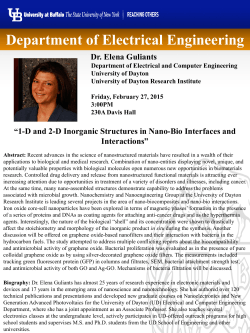


© Copyright 2026