
Effects of Test Variability - 2000 AAPT TTI
EFFECTS OF TEST VARIABILITY ON MIXTURE VOLUMETRICS AND MIX DESIGN VERIFICATION Authors: Adam J. Hand1 Amy L. Epps2 December 1, 1999 Revised for Presentation and Publication 2000 Annual Meeting of the Association of Asphalt Paving Technologists Reno, NV, March 2000. 1 . Assistant Professor, School of Civil Engineering, Purdue University, 1284 Civil Engineering Building, West Lafayette, IN 47907-1284, (765) 496-3996, email: [email protected]. 2 . Assistant Professor, Department of Civil Engineering, Texas A&M University, CE/TTI Building Room 503F, College Station, TX 77843-3136, (409) 862-1750, email: [email protected]. A. Hand and A. Epps ii ABSTRACT All currently used hot mix asphalt (HMA) mix design methods in the U.S. incorporate volumetric criteria. Volumetric properties are calculated from properties of both constituent materials and the combined asphalt-aggregate mixture which are determined through laboratory testing. Significant variability can be associated with these tests as noted in AASHTO and ASTM precision statements. A review of the precision statements associated with HMA mix design was performed and recommendations were made to help reduce this variability. Monte Carlo Simulation was used to ascertain the combined effects of variability in materials and mixture property measurements on volumetrics and optimum asphalt content (AC) selection. The results showed that within and between laboratory differences in air voids (AV) of approximately 1.0 and over 2.0 percent, respectively, at any given AC are likely when all testing is performed within the precision outlined in ASTM standards. These differences translate into potential differences in selected optimum AC of 0.7 percent and 1.4 percent for the within and between laboratory conditions, respectively. These potential differences will undoubtedly lead to problems when mix design verifications are performed in accordance with new types of specifications (end result and performance related) presently being implemented. This raises an urgent need for mix design verification criteria and specifications. A methodology is presented that could be used to develop such criteria and specifications. Key Words: HMA Volumetrics, Variability, Precision and Bias, Superpave, HMA Mix Design, Mixture Verification iii A. Hand and A. Epps TABLE OF CONTENTS Abstract ............................................................................................................................... ii Table of Contents ............................................................................................................... iii List of Abbreviations ...........................................................................................................v Introduction ..........................................................................................................................1 Mixture Volumetrics ............................................................................................................4 Mix Design Volumetric Requirements ................................................................................5 Precision and Bias Statements .............................................................................................6 Precision of Test Methods Related to HMA Volumetric.....................................................8 Bulk Specific Gravity of Compacted Specimens (Gmb) .....................................................9 Theoretical Maximum Specific Gravity of Loose Mix (Gmm) ...........................................9 Coarse Aggregate Bulk Specific Gravity (Gsb).................................................................10 Fine Aggregate Bulk Specific Gravity (Gsb).....................................................................10 Asphalt Binder Specific Gravity (Gb) ...............................................................................11 Monte Carlo Simulation Techniques .................................................................................11 Effects of Test Variability on Mixture Volumetrics ..........................................................13 Data Analysis .....................................................................................................................15 Within Lab Analysis ..........................................................................................................15 Between Lab Analysis .......................................................................................................19 Summary and Conclusions ................................................................................................21 References ..........................................................................................................................23 Appendix A. HMA Volumetric relationships ....................................................................41 LIST OF TABLES Table 1. Test methods and AASHTO and ASTM designations ........................................25 Table 2. Properties employed in volumetric calculations ..................................................25 Table 3. Superpave air void/percent compaction criteria ..................................................25 Table 4. Superpave VMA criteria .....................................................................................25 Table 5. Superpave VFA criteria ......................................................................................26 Table 6. Marshall mix design AV and VFA criteria ..........................................................26 Table 7. Marshall mix design VMA criteria ......................................................................26 Table 8. Summary of relevant AASHTO and ASTM single operator precision statements ............................................................................................................27 Table 9. Summary of relevant AASHTO and ASTM multilaboratory precision Statements ...........................................................................................................27 Table 10.Mix design summary ..........................................................................................28 Table 11.Summary of measured material properties and standard deviations used in within laboratory simulation...................................................................28 Table 12.Summary of measured material properties and standard deviations used in between laboratory simulation ...............................................................28 Table 13. Summary statistics based on within laboratory simulation ...............................29 Table 14. Summary statistics based on between laboratory simulation ............................30 Table15. Potential range of differences in optimum asphalt content and related volumetric properties for the within laboratory condition ..................................31 Table 16. Potential range of differences in optimum asphalt content and related volumetric properties for the between laboratory condition ...............................31 iv A. Hand and A. Epps LIST OF FIGURES Figure 1. Normal probability distribution of Gmb at 5.75% AC for within laboratory conditions ............................................................................................................32 Figure 2. Normal probability distribution of Gmb at 5.75% AC for within laboratory conditions ............................................................................................................32 Figure 3. Illustration of simulation used to generate %AV distribution ............................33 Figure 4. Air void distribution for within lab conditions at 5.75% AC .............................34 Figure 5. Air void distribution for between lab conditions at 5.75% AC ..........................34 Figure 6. Illustration of principles used in summary plots ................................................35 Figure 7. Air void summary as a function of asphalt content (within laboratory).............36 Figure 8. VMA summary as a function of asphalt content (within laboratory) .................36 Figure 9. VFA summary as a function of asphalt content (within laboratory) ..................37 Figure 10. %Gmmd summary as a function of asphalt content (within laboratory) ..........37 Figure 11. Dust proportion summary as a function of asphalt content (within laboratory) .........................................................................................................38 Figure 12. Air void summary as a function of asphalt content (between laboratory) .......38 Figure 13. VMA summary as a function of asphalt content (between laboratory)............39 Figure 14. VFA summary as a function of asphalt content (between laboratory) .............39 Figure 15. %Gmmd summary as a function of asphalt content (between laboratory) .......40 Figure 16. Dust proportion summary as a function of asphalt content (between laboratory) .........................................................................................................40 v A. Hand and A. Epps LIST OF ABBREVIATIONS Abbreviation Definition AASHTO American Association of State Highway and Transportation Officials AC Asphalt content, % by total weight of mixture AMRL AASHTO Materials Reference Laboratory ASTM American Society of Testing and Materials AV Mixture air voids, % DP Dust proportion FHWA Federal Highway Administration Gb Asphalt binder specific gravity Gmb Mixture bulk specific gravity Gmm Mixture theoretical maximum specific gravity %Gmmi Percent compaction at initial number of gyrations %Gmmd Percent compaction at design number of gyrations %Gmmm Percent compaction at maximum number of gyrations Gsa Aggregate apparent specific gravity Gsb Aggregate bulk (dry) specific gravity Gse Aggregate effective specific gravity HMA Hot mix asphalt Pa Air void content, % Pb Asphalt binder content, % by total weight of mixture Pba Absorbed binder, % by weight of aggregate Pbe Effective binder content, % by total weight of mixture Pmm Total loose mixture, % by total weight of mixture = 100 Ps aggregate, % by total weight of mixture RICE Mixture theoretical maximum specific gravity SHRP Strategic Highway Research Program Superpave Superior performing asphalt pavements VFA Voids filled with asphalt, % VMA Voids in mineral aggregate, % A. Hand and A. Epps 0 A. Hand and A. Epps 1 INTRODUCTION The current industry trend toward the implementation of end result and performance related specifications is placing primary mix design responsibilities with the contractor. Verification by the owner (eg. State Highway Department) of the optimum mixture selected by the contractor, according to the specified mix design method, is still required in this process. However, most of the responsibility for mix design is being transferred away from the State agency. With this change in responsibility, there is an urgent need to establish criteria or specifications for mix design verification. Verification criteria cannot be simply left to the discretion of state agency personnel. Instead, these criteria must be standardized and they must recognize the variability associated with determining the parameters used in verifying the mix design. This new system forces the contractor to assume the risk that the mix design will be approved. If the mix design is not verified, loss of productivity, time, and money are certain. It is likely that verification might be denied due to a set of criteria or specifications that are not sensitive to the variability in volumetrics that can result from variability associated with tests used to determine material properties that are ultimately used to calculate volumetrics. Inclusion of volumetrics in hot mix asphalt (HMA) mix design has long been suggested as necessary to ensure adequate field performance. All HMA mix design methods currently used in the U.S. incorporate volumetric criteria. To establish optimum asphalt content (AC), traditional Hveem and Marshall mix design methods rely on the combination of volumetrics and mechanical mixture tests. (1). Both design methods include air void (AV) content requirements, and the Marshall method specifies acceptable ranges of voids in the mineral aggregate (VMA) and voids filled with asphalt (VFA). In the Superpave volumetric mix design method, optimum AC selection is based entirely on volumetric properties (2,3). Criteria are placed on AV, VMA, VFA, percent compaction at initial (%Gmmi) and maximum (%Gmmm) numbers of gyrations, and dust proportion (DP). Most agencies currently specify 6 to 8 percent in-place AV for HMA, at the completion of construction. Mixture durability is improved when in-place AV are less than approximately 8 percent (4). A mixture placed at 8 percent AV will then typically undergo further densification due to traffic loading. Research has shown that in-place AV, after traffic densification, should be A. Hand and A. Epps 2 greater than approximately 3 percent to ensure sufficient HMA resistance to rutting (5). The corresponding optimum mixture compacted in the laboratory for mix design purposes contains 3 to 5 percent AV according to Marshall criteria, at least 4 percent AV according to Hveem criteria, and exactly 4.0 percent according to Superpave criteria. The theory behind these mix design air void criterion is that the optimum AC should be selected at the density which is expected in the field mixture after the design level of traffic has been applied. Adequate VMA, or the space occupied by both air and effective binder not absorbed by the aggregate, is specified in mix design methods to guard against durability problems when VMA is too large and instability when VMA is too small, resulting in inadequate room for binder expansion when temperatures increase. By specifying both AV and VMA, VFA is also controlled because the three volumetric parameters are interrelated. VFA is simply the percentage of the VMA filled with asphalt cement. VFA specifications are directed toward durability and are actually redundant if both AV and VMA criteria are specified. Percent compaction criteria at the initial and maximum number of gyrations, %Gmmi and %Gmmm, respectively, are included in the Superpave mix design method. %Gmmi is a measure of mixture compactibility and is included to identify mixtures that would be tender during construction and could be unstable under initial traffic loading. Criteria is placed on %Gmmm in an effort to identify mixtures that might possibly compact to an unacceptably low AV level under traffic. An acceptable range of dust proportion (DP) is also currently included in the Superpave specifications. DP is defined as the ratio of the amount of material passing the 0.075mm (p0.075mm) sieve to the effective asphalt content (AC). All of the volumetric parameters described are calculated values. None are directly measured. In order to calculate the volumetric parameters for a given mixture, the following six properties are required: 1. asphalt content (AC) and thus mix proportions; 2. asphalt cement specific gravity (Gb); 3. combined aggregate bulk specific gravity (Gsb); 4. bulk specific gravity of compacted specimens (Gmb); 5. theoretical maximum specific gravity of the mixture (Gmm); and A. Hand and A. Epps 3 6. the amount of material passing the 0.075mm sieve (p0.075mm). The American Society of Testing and Materials (ASTM) and the American Association of State Highway and Transportation Officials (AASHTO) both have well established test methods for measuring these properties (6,7,8). Unfortunately, there is a tremendous amount of variability associated with the measurement of these properties that are ultimately used to calculate volumetrics in the mix design process. This variability has a significant impact on the calculated mixture volumetrics, and this in turn can substantially affect the optimum mixture selected through any particular mix design method. Variability associated with measuring the properties required to calculate mixture volumetrics can create problems within a given laboratory, but it is even more troublesome when comparing mix designs between laboratories. When mix designs between laboratories do not agree, differences in the properties measured (eg. Gb, Gsb, Gmb, and Gmm) by each laboratory are usually compared with the acceptable range to two results (d2s) found in ASTM or AASHTO precision statements. The "difference two-sigma limit" (d2s) has been selected by ASTM as the appropriate index of precision for establishing the acceptable difference in two results. The index provides a maximum acceptable difference between two results on test portions of the same material. The d2s index equals the difference between two individual test results that would be equaled or exceeded in the long run in only 1 case of 20 (5 percent of the time) under the normal and correct operation of the test method (6). When d2s criteria are considered, the difference between data from two laboratories are usually within the limits, suggesting that the tests were properly conducted. There is currently no method available to evaluate the effect of the differences between laboratories in terms of volumetric properties. This leaves the question as to which mix design is correct or should be used. The problem is that it is very difficult to ascertain the combined effect of the variability associated with each measured property on the calculated volumetric properties. This paper illustrates possible differences that can exist in calculated mixture volumetrics and optimum mix design volumetric properties when the material properties (Gb, Gsb, Gmb, and Gmm) used to establish the volumetrics are determined within the requirements of the precision A. Hand and A. Epps 4 statements associated with the corresponding ASTM and AASHTO test methods used to measure them. The objective of the paper is to show the effect of what is considered acceptable variability in Gb, Gsb, Gmb, and Gmm measurements on mixture volumetrics for both within and between laboratory conditions. Data from a coarse 19mm nominal size Superpave mix design is used, along with the single-operator and multilaboratory standard deviations presented in ASTM and AASHTO precision statements, in Monte Carlo Simulations to generate the potential range of volumetric properties that could be observed for the given test results and test method variability. Based on a series of analyses of this type, volumetric mix design verification criteria can be developed. Background information is provided on calculation of volumetric parameters, volumetric requirements of different mix design systems, precision and bias statements, and the methodology used to perform the statistical analyses (Monte Carlo Simulations). This is followed by results of the analysis of the effect of variability in Gb, Gsb, Gmb, and Gmm measurements on mixture volumetrics for both within and between laboratory conditions. The effects on individual volumetric properties and the overall mix design are presented, and summary and conclusions complete the paper. MIXTURE VOLUMETRICS All of the fundamental relationships used to perform volumetric calculations are presented in Appendix A, assuming that reclaimed asphalt pavement (RAP) is not incorporated in the design. Recall that a total of six properties are required to perform volumetric calculations. In the mix design process AC and p0.075mm sieve are known quantities controlled in the laboratory. In other words, they do not have to be determined. The four other properties (Gb, Gsb, Gmb, and Gmm) must be determined in accordance with the appropriate test methods. The ASTM and AASHTO test methods used to measure these properties are summarized in Table 1. Five test methods are listed because two methods are required to measure Gsb, one each for the coarse and fine aggregate fractions. The coarse fraction is that portion of the aggregate retained on the 4.75mm sieve, while the fine fraction is the portion that passes the 4.75mm sieve. Asphalt cement specific gravity (Gb) must be measured for the binder that will be employed during construction, and Gsb of both the coarse and fine aggregate fractions of the combined aggregate A. Hand and A. Epps 5 must be measured independently. The Gsb used in volumetric calculations is the weighted average of the coarse and fine fraction Gsb values. The bulk specific gravity of each specimen compacted during the mix design process (Gmb) must be measured, and the theoretical maximum specific gravity (Gmm) of the loose mixture at one AC must be determined. The Gmm of the mixture at other asphalt contents considered in the mix design process may then be calculated after determining the effective specific gravity of the aggregate (Gse) from the measured Gmm. A review of the information presented in Appendix A reveals the relationships between volumetric properties and the two zero variability (AC and p200) and four measured properties employed in volumetric calculations. Table 2 summarizes these relationships. MIX DESIGN VOLUMETRIC REQUIREMENTS All commonly used HMA mix design methods incorporate volumetric criteria. The Superpave volumetric mix design method relies entirely on six volumetric criteria for optimum AC selection (2, 3, 9). These criteria for AV, VMA, VFA, %Gmmi, %Gmmm, and DP are summarized in Tables 3, 4, and 5. The AV, VMA, VFA, and DP criteria all apply at the design number of gyrations. Regardless of traffic, environmental conditions, and materials, the AV criteria is fixed at 4.0 percent. Optimum AC is the AC at which the AV of the compacted mixture are equal to 4.0 percent (96.0 percent of Gmm) at the design number of gyrations. The VMA criteria is a function of nominal maximum aggregate size, while the VFA criteria is a function of expected traffic. The DP criteria is 0.6 to 1.2 for all mixtures. The required values for percent compaction at the initial (%Gmmi) and maximum (%Gmmm) number of gyrations are less than 89 and 98 percent, respectively, for all mixtures. In addition to Marshall stability and flow requirements, three volumetric criteria are incorporated in the Marshall mix design method, including AV, VMA, and VFA (1). These criteria are summarized in Tables 6 and 7. AV and VFA criteria are a function of traffic, while VMA criteria is a function of nominal maximum particle size and design AV. A. Hand and A. Epps 6 The Hveem mix design method relies on mixture stability and observations of flushing for selection of optimum AC and does not specifically incorporate volumetric requirements. However, the following note is presented in the Asphalt Institutes Manual Series 2 (MS-2), “Although not a routine part of this design method, an effort is made to provide a minimum percent of air voids of approximately 4 percent” (1). Some State agencies that specify the Hveem design method, for example Nevada Department of Transportation, also incorporate limited volumetric criteria (10). PRECISION AND BIAS STATEMENTS When tests are performed on presumably identical materials under presumably identical circumstances, it is not likely that identical results will be obtained. The difference in results is attributed to unavoidable random errors that are inherent in every test method. In other words, all the factors that influence the outcome of a test can not be completely controlled. For practical interpretation of test results, this inherent variability must be taken into account. As an example, the difference between a test result and some specified value might be within that which can be expected due to unavoidable random error, in which case real deviation from the specified value has not been demonstrated. Similarly, the difference between test results from two batches of material will not indicate a fundamental quality difference if the difference is no greater than that which may be attributed to inherent variability in the test procedure. Several factors may contribute to the variability associated with the application of a test method, including the following: 1. the operator; 2. the equipment used; 3. equipment calibration; and 4. the environment. The degree to which each factor contributes to the variability associated with individual test methods is dependent on the specific test method. For example, temperature is critical in determining aggregate specific gravity, but it is irrelevant in determining coarse aggregate angularity. A. Hand and A. Epps 7 All ASTM and AASHTO test methods incorporate a section on precision that addresses inherent test method variability. Within the precision section, test method precision and bias statements are given. Notes are also typically provided which define the interlaboratory test program employed to formulate the statements. Some relatively new test methods will lack precision statements because they have not yet been developed. ASTM C670, "Standard Practice for Preparing Precision and Bias Statements for Test Methods for Construction Materials," provides guidance in preparing precision and bias statements for ASTM test methods pertaining to certain construction materials (6). The standard also provides recommended forms for precision and bias statements. ASTM C802, "Conducting an Interlaboratory Test Program to Determine the Precision of Test Methods for Construction Materials," is the companion method that states the requirements for the interlaboratory test program which generates the data to be analyzed and presented in accordance with ASTM C670. ASTM and AASHTO precision statements contain estimates of single-operator precision and multilaboratory precision. Single-operator precision is a measure of the greatest difference between two results that would be considered acceptable when properly conducted repetitive determinations are made on the same material by a single competent operator. Multilaboratory precision is a measure of the range (greatest difference between two test results) that would be considered acceptable when properly conducted determinations are made by two different operators in different laboratories on portions of a material that were intended to be identical, or at least as nearly identical as possible. Single-operator precision is sometimes referred to as "repeatability" or “within laboratory” precision, while multilaboratory precision is sometimes referred to as "reproducibility" or “between laboratory” precision. A description of the statistical terms incorporated in precision and bias statements is presented in Section 3.0 of ASTM C670 (6). The fundamental statistic underlying all indices of precision is the standard deviation of the population of measurements, termed the "one-sigma limit" (1s). It is an indication of the variability of a large group of individual test results obtained under similar conditions. One-sigma limits (1s) are determined for both single-operator and multilaboratory conditions. A. Hand and A. Epps 8 Precision statements also include a section presenting an acceptable range of results. The "difference two-sigma limit" (d2s) has been selected by ASTM as the appropriate index of precision for establishing the acceptable difference between two results. The index provide a maximum acceptable difference between two results on test portions of the same material. The d2s index equals the difference between two individual test results that would be equaled or exceeded in the long run in only 1 case of 20 (5 percent of the time) under the normal and correct operation of the test method. The d2s index is determined by multiplying the 1s by a factor of 22 or 2.828, and this actually represents the 95 percent confidence interval. Bias may be defined as systematic error inherent in the test method that contributes to the difference between a population mean of the measurements or test results and an accepted reference or true value. In all test methods, tolerances are placed on the accuracy of measuring equipment. All tests performed with a given set of equipment which has an error within the permitted tolerance will produce results with a small consistent bias, but the bias is not inherent in the test method, nor is it included in the bias statement for the method. Two conditions which permit the bias of a test method to be established are: 1. a standard reference sample of known value has been tested using the test method; and 2. the test method has been applied to a sample which has been compounded in a manner such that the true value of the property being measured is known. Determining whether a potential reference sample is suitable for the purpose requires judgement. Rarely is there a reference material available for most test methods. When a reference is not available, that must be stated along with a statement indicating that no statement can be made on bias. This is the case for all of the test methods associated with HMA mixture design. PRECISION OF TEST METHODS REQUIRED FOR DETERMINING VOLUMETRICS The five test methods used to measure the required material properties employed in volumetric calculations along with their AASHTO and ASTM precision statements are listed in Tables 8 and 9, for single-operator and multilaboratory precision, respectively. Both the one-sigma limits (1s) and acceptable range of two results (d2s) statistics are presented. The AASHTO and ASTM precision statements are identical for four of the five test methods. The exception is the AASHTO T166 and ASTM D2726 test methods for measuring Gmb. The precision section in A. Hand and A. Epps 9 AASHTO T166 simply states, “Duplicate specific gravity results by the same operator should not be considered suspect unless they differ more than 0.02.” The “single-operator” portion of the statement suggests that this value is single-operator precision, and the remainder of the statement suggests that it is an acceptable range of two results condition. If this is the case, the one-sigma limit (1s) would be equal to 0.02 2.828 = 0.007, which is less than one half of the single-operator one-sigma limit (1s) stated in ASTM D2726. This is a major discrepancy between the two methods and the AASHTO test method lacks multilaboratory precision, rendering it useless for between laboratory comparisons (eg. contractor mix design verifications by the owner). Bulk Specific Gravity of Compacted Specimens (Gmb) The ASTM D2726 precision statement is based on 75 blow Marshall compaction of HMA produced in three bituminous mixing plants. Sixteen laboratories participated, each compacting four replicates of six different materials. The AASHTO Materials Reference Laboratory (AMRL) has accumulated test results for three rounds of HMA gyratory proficiency samples. The results include Gmb determinations on specimens compacted with the Superpave Gyratory Compactor (SGC) to the maximum number of gyrations. Although a precision statement has not yet been developed, the single-operator and multilaboratory one-sigma limits (1s) observed to date are approximately 0.01 and 0.025, respectively. These are very similar to those stated in ASTM D2726 (0.0124 and 0.0269) for the Marshall compacted specimens. This is somewhat alarming when one considers that the gyratory specimens were compacted to the maximum number of gyrations, which typically results in very low AV ( 2.0 percent). One would expect less variability for the gyratory compacted specimens because the AV in the specimens are very low. There is currently a recommendation that the compaction procedure in Superpave be modified to terminate compaction at the design number of gyrations for volumetric analysis instead of compacting to the maximum number of gyrations and back-calculating properties at the design number of gyrations (11). This will result in determining Gmb on specimens with greater AV, and it is very likely that the variability associated with these measurements will increase relative to the variability associated with measurements on specimens with lower AV. This will only lead to greater variability in volumetric properties in the future. A. Hand and A. Epps 10 Theoretical Maximum Specific Gravity (Gmm) Two sets of precision values are stated in Tables 8 and 9 from AASHTO T209 and ASTM D2041. The top number in each cell is the precision statement for non-porous aggregate conditions, and values are based on testing of three replicates for each of five materials by five laboratories. The lower number in each cell in parenthesis is the precision statement that reflects use of the supplemental procedure for mixtures containing porous aggregate, commonly known as the “dryback” procedure. These data are based on testing of two replicates for each of seven materials in twenty laboratories. Coarse Aggregate Bulk Specific Gravity (Gsb) The values stated in Tables 8 and 9 for coarse aggregate specific gravity (Gsb) (AASHTO T85 and ASTM C127) are based on an analysis of AMRL reference sample data with some laboratories using 15 hour minimum saturation times and other laboratories using 24 4 hour saturation times. The aggregates were all normal-weight, and the precision indices are based on aggregates with absorption of less than 2.0 percent, which is not always the case for aggregates used in HMA. Fine Aggregate Bulk Specific Gravity (Gsb) The values stated in Tables 8 and 9 for fine aggregate specific gravity (Gsb) (AASHTO T84 and ASTM C128) are based on an analysis of AMRL reference sample data with some laboratories using 15 to 19 hour saturation times and other laboratories using 24 4 hour saturation times. The aggregates were all normal-weight. The precision indices are based on an analysis of more than 100 paired test results from 40 to 100 laboratories on aggregates with absorption values of less than 1.0 percent and may differ for manufactured fine aggregates and fine aggregate having absorption values greater than 1.0 percent. It is actually common for HMA aggregates to be manufactured and to have absorption values much greater than 1.0 percent. An inherent problem with this test method is that highly fractured manufactured fine aggregates may not slump when in the saturated surface dry (SSD) condition. Internal friction prevents slumping until the aggregate reaches a condition much drier than SSD. This results in low measured Gsb values and greater variability. The reality is that it can be difficult to meet A. Hand and A. Epps 11 acceptable range of two results (d2s) precision criteria when testing the highly crushed manufactured fines required to meet Superpave fine aggregate consensus property requirements. The test method was initially developed for testing rounded concrete sands, and refinements or extensive revision for HMA aggregate testing purposes is recommended to help reduce variability introduced into volumetric calculations. Asphalt Binder Specific Gravity (Gb) The asphalt binder specific gravity (Gb) (AASHTO T228 and ASTM D70) precision stated in Tables 8 and 9 is specifically for asphalt cement tested at 25C. The test methods provide statements for asphalt cement, soft tar pitch, and asphalt cement and soft tar pitch pooled at both 25 and 60C. The method does not provide details of the interlaboratory study conducted to develop the precision statement, but it indicates that the single-operator data set for asphalt cement tested at 25C incorporated 54 degrees of freedom. The multilaboratory data set for the same conditions had 24 degrees of freedom. It is clear from a review of these precision statements that there is a need to refine or replace some of the test methods to help reduce variability in the measured properties. There is also a need to expand the data bases used to develop the precision statements, particularly for the Gsb test methods. Additionally, internal laboratory quality control, technician certification and laboratory accreditation should be given serious consideration within the industry. These issues along with addition data associated with test method variability are review in the sixty-fifth volume of the Journal of the Association of Asphalt Paving Technologists (12, 13,14). MONTE CARLO SIMULATION Monte Carlo Simulation techniques were used to determine the combined effects of the variability associated with Gb, Gsb, Gmb, and Gmm measurements on mixture volumetrics. These techniques have been applied in other pavement/materials engineering applications, particularly in the research environment, and have been reported in the Journal of the Association of Asphalt Paving Technologists (AAPT) (15). 12 A. Hand and A. Epps The simplest method of describing Monte Carlo Simulation is by example. Consider the calculation of percent AV. The following relationship is used to calculate percent AV: %AV = 100 G mm G mb G mm (1) where: %AV = air voids in compacted mixture, percent of total volume Gmm = maximum specific gravity of paving mixture Gmb = bulk specific gravity of compacted mixture Percent AV is a function of both the bulk specific gravity of the compacted mixture (Gmb) and the theoretical maximum specific gravity of the mixture (Gmm). Given measured values for each of these properties (mix design data in this case) and the standard deviation (1s or one-sigma limits in the AASHTO or ASTM precision statements) associated with each of the tests used to measure the properties, normal probability distributions are developed for each property. Such normal distributions for Gmb using both within and between laboratory precision are illustrated in Figures 1 and 2. The Gmb measured at 5.75% AC (2.336 in Table 10) in the mix design is used along with the ASTM standard deviations (1s) for Gmb under within (0.0124) and between (0.0269) laboratory conditions which are presented in Tables 8 and 9, respectively. Note the overall appearance of Figures 1 and 2 are similar and the mean value () of both distributions are equal (2.336), however the standard deviations are quite different. The standard deviation for the between laboratory condition is much larger (0.0269 versus 0.0124). A close review of the values along the x-axis of each plot reveals that the width of the between laboratory distribution is actually over two times that of the within laboratory distribution as would be expected. Once the Gmb and Gmm normal distributions have been established, they are repeatedly sampled in a random fashion. With each sample of Gmb and Gmm, AV is calculated using Equation 1. A distribution of AV is eventually generated after taking multiple (thousands) samples and calculating corresponding AV values. The AV distribution produced represents the combined effects on AV of the variability associated with Gmb and Gmm measurements. This is illustrated graphically in Figure 3. The Gmb and Gmm distributions are termed “simulation inputs”, and the AV distribution is termed the “simulation output.” A. Hand and A. Epps 13 The key to this process is the repeated sampling of the input probability distributions and calculation of output distribution data. Sampling is the process by which values are randomly drawn or selected from input probability distributions. The Monte Carlo sampling technique was employed in the simulations presented (16). This technique is entirely random, which means that any given sample may fall within the range of the input distributions. Each time the input distributions are sampled and an output data point is calculated is termed an iteration. With enough iterations, the sampled values for a probability distribution become distributed in a fashion that approximates the known input probability distribution. The statistics of the sampled distribution approximate the true statistics for the input distribution. The same holds true for the output distribution, with enough iterations; the statistics of the output distribution approximate the true statistics for the output distribution. Therefore it is critical that an adequate number of iterations are performed. Convergence monitoring can be performed during a Monte Carlo Simulation to track the stability of the output distributions generated (17). As greater and greater numbers of iterations are executed during a simulation, the output distributions generated become more “stable.” Distributions become more stable because the statistics that describe them change less and less as additional iterations are performed. The total number of iterations required to generate a stable output distribution is dependent on the complexity of the model being simulated and the distribution functions employed in the model. Monitoring convergence insures that a sufficient number of iterations are performed. The method used to monitor convergence for the simulations presented in this paper was as follows. After every 100 iterations, three statistics were calculated for each output distribution, including the mean, standard deviation, and percentiles (0 percent to 100 percent in 5 percent increments). Each time new statistics were calculated (every 100 iterations), the percent change in the statistics from the prior calculation was determined. As the percent change decreases, the impact on the statistics of running additional iterations decreases and the output distributions become more stable. When compared to typical values of 1.0 or 1.5 percent, the selected convergence threshold of 0.75 percent was conservative. In other words when all three statistics changed less than 0.75 percent for two consecutive sets of calculations, the simulation was terminated. A. Hand and A. Epps 14 EFFECTS OF TESTING VARIABILITY ON VOLUMETRICS Test results associated with a Superpave mix design were used, along with the single-operator and multilaboratory precision values presented in Tables 8 and 9, in Monte Carlo Simulations to generate the potential range of volumetric properties that could be observed for the given test results and test method variability. The Superpave mix design employed in the analyses incorporated a PG64-22 binder and 100 percent crushed aggregate. The blended aggregate gradation was a coarse (plotted below the restricted zone) 19mm nominal size with 38 percent passing the 4.75mm sieve. The mixture was designed as a surface course with expected traffic of 10 to 30x106 equivalent single 80kN axle loads (ESALs). The environment it was designed for had an average design high air temperature of <39C. The mixture met all of the Superpave volumetric mix design requirements at the optimum asphalt content of 5.75 percent. The mix design volumetrics are summarized in Table 10, with the volumetrics at the optimum AC highlighted. Two simulations were conducted. One was performed for within laboratory conditions and another was performed for between laboratory conditions. The same Superpave mix design data was used in both simulations to represent mean data. Each simulation incorporated four asphalt contents. The mix design data was coupled with the appropriate standard deviations (1s) from ASTM precision statements (within laboratory = single-operator precision and between laboratory = multilaboratory precision). The material properties and standard deviations employed in the within laboratory and between laboratory simulations are presented in Tables 11 and 12, respectively. These are the data that were used to generate the input distributions from which the output distributions were determined. Weighted averages of coarse and fine aggregate Gsb standard deviations were used to establish the standard deviations for the blended aggregate Gsb used in the simulations. Sixty-two percent of the combined aggregate blend was retained on the 4.75mm sieve, therefore 38 percent passed the 4.75mm sieve. This information along with the coarse and fine aggregate Gsb standard deviations reported in Tables 7 and 8 were entered into Equation A1 of Appendix A to establish the within and between laboratory Gsb standard deviations reported in Tables 11 and 12. A. Hand and A. Epps 15 A theoretical maximum specific gravity (Gmm) was measured at 5.75 percent AC during the mix design process. Gmm testing was not conducted at other asphalt contents. Therefore the simulations incorportated the calculation of Gmm values at asphalt contents other than 5.75%. This process is representative of the method most commonly used in HMA mix design. DATA ANALYSIS Thirty-six output distributions were generated for each simulation. The results associated with twenty of these distributions are reported in this section. They include AV, VMA, VFA, Gmmd, and DP at each of four asphalt contents. The output not reported is associated with intermediate calculations, which included Pba, Pbe, Gse, and Gmm at asphalt contents other than 5.75 percent. Figures 4 and 5 are output distribution examples for AV at the optimum AC (5.75 percent) for the within and between laboratory conditions, respectively. The data are reasonable and logical in that the mean of each distribution is equal and the range of between laboratory data is much greater than the within laboratory data. The data are also extremely disturbing in that they show the potential for tremendous differences in AV when variability in Gmb and Gmm test results is within the levels currently allowed in AASHTO and ASTM standards. These distributions are typical of the other output distributions observed. In the interest of brevity, all of the output distributions are not presented. Summary statistics are extracted from them and presented in tables and plots. Within Laboratory Analysis The within laboratory simulation data are summarized in Table 13. For each volumetric property at each AC, the following distribution statistics are presented: 1. mean; 2. standard deviation; 3. minimum observation ; 4. maximum observation; 5. volumetric property values at plus and minus one standard deviation from the mean (+1 Std Dev and –1 Std Dev); A. Hand and A. Epps 16 6. volumetric property values at plus and minus two standard deviations from the mean (+2 Std Dev and –2 Std Dev); and the 7. 5th, 10th, 25th, 50th, 75th, 90th, and 95th percentiles. These 15 statistics can be viewed in a number of ways, however the remainder of the paper will focus on means, volumetric properties at plus and minus one standard deviation from the mean, and the 5th and 95th percentiles. The mean is the average property value, and sixty-eight percent of the observations lie within plus and minus one standard deviation of the mean for normally distributed data (16). Only 5 percent of the observations lie below the 5th percentile, and 95 percent of the observations lie below the 95th percentiles. One other interesting pair of statistics are the 25th and 50th percentiles in that 50 percent of the observations lie between them. The rational for selecting these statistics is simply that the bulk of the observations are within one standard deviation of the mean and the 5th and 95th percentiles represent reasonable extremes. They are analogous to being at the extremes of an ASTM acceptable range of two results (d2s) limit. The means, volumetric properties at plus and minus one standard deviation from the mean, and the 5th and 95th percentiles are plotted as a function of AC for the within laboratory data in Figures 7 through 11. The data presented in the plots are highlighted in Table 13. The plots are an attempt to summarize all of the selected statistics over a range of asphalt contents. The ideal situation would be to plot the complete distribution at each AC as illustrated in Figure 6. However, it is difficult to surmise where the important statistics lie within each distribution on such a small scale, thus Figures 7 through 11 are provided. Figure 7 shows that the range of AV within one standard deviation of the mean is just over 1.0 percent regardless of AC (eg. 3.5 to 4.6 percent at 5.75 percent AC) and the range between the 5th and 95th percentiles is approximately 1.8 percent. This shows that two different technicians working in the same laboratory with the same materials and equipment and conducting all testing within the precision outlined in ASTM standards could each perform a mix design and could reasonably report differences in AV of 1.8 percent at any given AC. It is likely that they would report differences of just over 1.0 percent. Another way of interpreting the AV data in Table 13 is to say that fifty percent of the time two different technicians working in the same laboratory A. Hand and A. Epps 17 and performing replicate mix designs may report a difference in AV at any given AC of up to 0.7 percent. This statement is based on the difference in the 25th and 75th percentiles, between which fifty percent of the test results would lie. The range of VMA shown in Figure 8 within one standard deviation of the mean is about 0.9 percent regardless of AC (eg. 14.8 to 15.9 percent at 5.75 percent AC) and the range between the 5th and 95th percentiles is approximately 1.8 percent. This shows that two different technicians working in the same laboratory with the same materials and equipment could each perform a mix design and could reasonably report differences in VMA of 1.8 percent at any given AC. It is likely that they would report differences of approximately 0.9 percent. The difference in the 25th and 75th percentiles presented in Table 13 is 0.7 percent. In other words, fifty percent of the time two different technicians working in the same laboratory performing replicate mix designs may report differences in VMA at any given AC of up to 0.7 percent. VFA ranges approximately 5.5 percent within one standard deviation of the mean, and the range between the 5th and 95th percentiles is about 9.0 percent (Figure 9). This shows that the two different technicians could reasonably report differences in VFA of 9.0 percent at any given AC. It is likely that they would report differences of approximately 5.5 percent. The difference in the 25th and 75th percentiles for VFA in Table 13 is about 3.8 percent. Therefore, fifty percent of the time two different technicians working in the same laboratory performing replicate mix designs may report differences in VFA at any given AC of up to 3.8 percent. The %Gmmd data is presented in Figure 10 but will not be discussed as results are identical to those of the AV data. However, the data is presented in this form for completeness. Figure 11 shows that dust proportion (DP) is much more sensitive to AC than the other volumetric properties. The range of DP within one standard deviation of the mean progressively decreases with AC from 0.09 to 0.05, and the range between the 5th and 95th percentiles progressively decreases with AC from 0.14 to 0.08. This shows that the two different technicians could reasonably report differences in DP of 0.11 on average. It is likely that they would report A. Hand and A. Epps 18 differences of up to 0.07 on average. Fifty percent of time the different technicians would report DP differences of up to approximately 0.05. Another important way of analyzing this data is in terms of the differences that could be observed in optimum AC selection. Table 15 summarizes the differences for the within laboratory condition. The data in the table were obtained by entering Figure 7 at 4.0 percent AV and moving horizontally to the right to the intersection of the lines representing the mean, plus and minus one standard deviation, and the 5th and 95th percentiles. At each intersection a line was drawn vertically down to the x-axis, and the corresponding “optimum” AC associated with each statistic was obtained. The VMA, VFA, %Gmmd, and DP plots were then entered at the appropriate “optimum” asphalt contents to obtain the corresponding volumetrics presented in Table 15. This is the exact same process used in the Superpave mix design system. At one standard deviation below the mean AV level, an optimum AC of 5.52 percent would be selected. This value is only 0.23 percent less than the mean AC. The corresponding changes in VMA and VFA are reductions of 0.6 and 5.9 percent from the mean, respectively. At the 5th percentile level of AV an optimum AC of 5.33 percent would be selected, 0.42 percent below the mean. Corresponding changes in VMA and VFA from the mean are reductions of 1.0 and 10.4 percent, respectively. The mix is more sensitive at AV levels above the mean. This is very reasonable when one considers the typical form of the relationship between AV and AC. An optimum AC of 6.29 percent would be selected at one standard deviation above the mean AV level. This differs from the mean by an increase of 0.54 percent. The corresponding changes in VMA and VFA are increases of 1.2 and 7.4 percent from the mean, respectively. At the 95th percentile AV level, an optimum AC of greater than 6.75 percent would be selected, at least a full percent greater than the mean. The VMA and VFA at that AC are greater than 17.2 and 88 percent, respectively. These values are reported as “greater than” because the 95th percentile AV trend does not intersect 4.0 percent (Figure 7) and data were only available up to 6.75 percent AC. In summary, the data show that two different technicians working in the same laboratory with the same materials and equipment could each perform a mix design and could report differences in A. Hand and A. Epps 19 optimum AC of over 1.4 percent (>6.75-5.33), differences in VMA of over 2.9 percent (>17.214.3), and differences in VFA of 20 percent (>88-67.9). It is likely that they would report differences in optimum AC of up to 0.8 percent (6.29-5.52), differences in VMA of up to 1.8 percent (16.5-14.7), and differences in VFA of up to 13 (81.2-67.9) percent. Between Laboratory Analysis The between laboratory data are summarized in Table 14. The same analysis that was made on the within laboratory data was also performed on the between laboratory data. The means, volumetric properties at plus and minus one standard deviation from the mean, and the 5th and 95th percentiles are plotted as a function of AC for the between laboratory data in Figures 12 through 16. The data presented in the plots are highlighted in Table 14. Figure 12 shows that the range of AV within one standard deviation of the mean is 2.2 percent regardless of AC and the range between the 5th and 95th percentiles is approximately 3.7 percent. This shows that two laboratories working with the same materials and equipment and conducting all testing within the precision outlined in ASTM standards could each perform a mix design and could reasonably report differences in AV of 3.7 percent at any given AC. It is likely that the laboratories would report differences of 2.2 percent. Another interpretation of the AV data in Table 14 is to say that fifty percent of the time two different laboratories working with the same materials and performing all testing within the precision outlined in ASTM standards may report differences in AV at any given AC up to 1.5 percent. This statement is based on the difference in the 25th and 75th percentiles, between which fifty percent of the test results would lie. The range of VMA shown in Figure 13 within one standard deviation of the mean is 2.2 percent regardless of AC, and the range between the 5th and 95th percentiles is approximately 3.6 percent. This shows that two different laboratories working with the same materials could each perform a mix design and could reasonably report differences in VMA of 3.6 percent at any given AC. It is likely that they would report differences of approximately 2.2 percent. The difference in the 25th and 75th percentiles presented in Table 14 for VMA is 1.5 percent. In other words, fifty percent of the time two different laboratories performing replicate mix designs may report differences in VMA at any given AC of up to 1.5 percent. A. Hand and A. Epps 20 VFA ranges approximately 11.8 percent within one standard deviation of the mean, and the range between the 5th and 95th percentiles is approximately 17.8 percent (Figure 14). This shows that the two different laboratories could reasonably report differences in VFA of 17.8 percent. It is likely that they would report differences of approximately 11.8 percent. The difference in the 25th and 75th percentiles for VFA in Table 14 is approximately 8.0 percent. Therefore, fifty percent of the time two different laboratories working with the same materials performing replicate mix designs may report differences in VFA of up to 8.0 percent. The %Gmmd data is presented in Figure 15 but will not be discussed as results are identical to those of the AV data. Again, the data is presented in this form for completeness. As noted in the within laboratory analysis, Figure 16 shows that dust proportion (DP) is more sensitive to AC than other volumetric properties. The range of DP within one standard deviation of the mean progressively decreases with AC from 0.14 to 0.08, and the range between the 5th and 95th percentiles progressively decreases with AC from 0.24 to 0.13. This shows that the two laboratories could reasonably report differences in DP of 0.19 on average. It is likely that they would report differences of 0.11 on average. Fifty percent of the time the different laboratories may report DP differences of up to approximately 0.08. Table 16 summarizes the data analysis in terms of the differences that could be observed in optimum AC selection for the between laboratory condition. The data in the table were obtained as previously discussed according to the exact same process used in the Superpave mix design method. At one standard deviation below the mean AV level, an optimum AC of 5.25 percent would be selected, 0.5 percent less than the mean AC. The corresponding changes in VMA and VFA are reductions of 1.2 and 12.3 percent from the mean, respectively. An optimum AC of 6.67 percent would be selected at one standard deviation above the mean AV level. This result differs from the mean by an increase of 0.92 percent. The corresponding changes in VMA and VFA are increases of 2.0 and 15.4 percent from the mean, respectively. At the 5th and 95th percentile AV A. Hand and A. Epps 21 levels, optimum AC and corresponding volumetrics are not reported because the 5th and 95th percentile AV trends do not intersect 4.0 percent AV in Figure 12. Due to the non-linearity of typical AV relationships, it is inappropriate to extrapolate the curves. In summary, the data show that two different laboratories working with the same materials and conducting all testing within the precision stated in ASTM standards could each perform mix designs and report differences in optimum AC of over 1.4 percent (6.67-5.25), differences in VMA of over 3.2 percent (17.314.1), and differences in VFA of over 28 percent (89.2-61.5). SUMMARY AND CONCLUSIONS Analyses presented show that variability associated with measurement of the properties required to determine mixture volumetrics can have significant impact on calculated volumetric properties. The data are extremely disturbing because they reveal the potential for tremendous differences in volumetrics when variability in Gb, Gsb, Gmb, and Gmm test results is within the limits currently allowed in AASHTO and ASTM standards. Monte Carlo Simulation was used to ascertain the combined effects of variability in these properties on volumetrics and optimum asphalt content (AC) selection in the mix design process. The data showed that two different technicians working in the same laboratory with the same materials and equipment and conducting all testing within the precision outlined in ASTM standards could each perform a mix design and it is likely that they could report differences in both AV and VMA of approximately 1.0 percent at any given AC. Data also show that two different laboratories working with the same materials and conducting all testing within the precision outlined in AASHTO and ASTM standards could each perform a mix design and it is likely that the laboratories would report differences in both AV and VMA of over 2.0 percent at any given AC. These differences would translate into potential differences in selected optimum asphalt contents of 0.7 percent and 1.4 percent for the within and between laboratory conditions, respectively. The effects of what is currently considered acceptable test variability on volumetrics and AC selection are unacceptable in light of the new types of specifications being implemented. These specifications place mix design responsibility on the contractor and mix design verification A. Hand and A. Epps 22 responsibility with the owner or agency. Verifying agencies are going to have to recognize the fact that variability exists and has a large potential impact to result in differences in mix design. This statement is also true for field management operations. This will ultimately drive the development of much needed mix design verification criteria and specifications. Monte Carlo Simulation is an effective technique for simulating volumetric property distributions resulting from test method variability. The application present in this paper could be used to develop mix design verification criteria and specifications. Review of the AASHTO and ASTM precision statements for the test methods associated with HMA mix design revealed a need for refinement or replacement of some of the test methods to help reduce variability in measured properties. There is also a need to expand the data bases used to develop the precision statements. The industry must concentrate on reducing test method variability. In addition to development of new methods and refinements to current methods, internal laboratory quality control, technician training and certification, and laboratory accreditation are all instruments that can assist with reducing test variability. A. Hand and A. Epps 23 REFERENCES 1. Asphalt Institute, " Mix Design Methods for Asphalt Concrete and Other Hot-Mix Types," Manual Series 2 (MS-2), Sixth Edition, Asphalt Institute, Lexington, Kentucky, 1993. 2. Federal Highway Administration, "Background of Superpave Asphalt Mixture Design and Analysis," Publication Number: FHWA-SA-95-003, Federal Highway Administration, Washington D.C., February 1995. 3. Harrigan, E.G., R.B. Leahy, and J.S. Youcheff, "The Superpave Mix Design System Manual of Specifications, Test Methods, and Specifications," SHRP-A-379, Strategic Highway Research Program, National Research Council, Washington, D.C., 1994. 4. Roberts, F.L., P.S. Kandhal, E.R. Brown, D.Y. Lee, and T.W. Kennedy, “Hot Mix Asphalt Materials, Mixture Design, and Construction,” Second Edition, National Asphalt Pavement Association, Lanham, Maryland, 1996. 5. Brown, E.R., and S.A. Cross, “A National Study of Rutting in Hot Mix Asphalt (HMA) Pavements,” Journal of the Association of Asphalt Paving Technologists, Volume 61, St. Paul, MN, 1992. 6. American Society of Testing and Materials, "Concrete and Aggregate," Annual Book of ASTM Standards, Section 4, Volume 04.02, American Society of Testing and Materials, West Conshohocken, PA, 1998. 7. American Society of Testing and Materials, " Road and Paving Materials; Vehicle-Pavement Systems," Annual Book of ASTM Standards, Section 4, Volume 04.03, American Society of Testing and Materials, West Conshohocken, PA, 1998. 8. American Association of State Highway and Transportation Officials, Standard Specifications for Transportation Materials and Methods of Sampling and Testing, 19th Edition, Part II, American Association of State Highway and Transportation Officials, Washington, D.C., 1998. 9. Cominsky, R.R., R.B. Leahy, and E.G. Harrigan, "Level One Mix Design: Materials Selection, Compaction, and Conditioning," SHRP-A-408, Strategic Highway Research Program, National Research Council, Washington, D.C., 1994. 10. Nevada Department of Transportation, “Materials Division Testing Manual,” Materials Division, Nevada Department of Transportation, Carson City, NV, April 1997. 11. Brown, E.R. and M.S. Buchanan, “Consolidation of the Ndesign Compaction Matrix and Evaluation of Gyratory Compaction Requirements,” Journal of the Association of Asphalt Paving Technologists, Volume 68, St. Paul, MN, 1999. A. Hand and A. Epps 24 12. Wolters, R.O., “Practical Issues Relating to Accreditation and Certification,” Journal of the Association of Asphalt Paving Technologists, Volume 64, St. Paul, MN, 1995. 13. Spellerburg, P.A., “AASHTO Accreditation for Bituminous Materials Testing Laboratories,” Journal of the Association of Asphalt Paving Technologists, Volume 64, St. Paul, MN, 1995. 14. Tahmoressi, M., “Hot Mix Technician Program in Texas,” Journal of the Association of Asphalt Paving Technologists, Volume 64, St. Paul, MN, 1995. 15. Harvey, J.T., T. Hoover, N.F. Coetzee, W.A. Nokes, and F.C. Rust, “CALTRANS Accelerated Pavement Test (CAL/APT) Program – Test Results: 1994-1997,” Journal of the Association of Asphalt Paving Technologists, Volume 67, St. Paul, MN, 1998. 16. Miller, I., F.E. Freud, and R.A. Johnson, "Probability and Statistics for Engineers," Prentice Hall, Englewood Cliffs, NJ, 1990. 17. “@RISK - Advanced Risk Analysis for Spreadsheets,” @RISK users manual, Palisade Corporation, Newfield, NY, July 1997. 25 A. Hand and A. Epps Table 1. Test methods and AASHTO and ASTM designations. Designations Description AASHTO ASTM Method Method T228 D70 Asphalt Cement Specific Gravity (Gb) T85 C127 Coarse Aggregate Specific Gravity (Gsb) T84 C128 Fine Aggregate Specific Gravity (Gsb) T166 D2726 Bulk Specific Gravity of Compacted Bituminous Specimens (Gmb) T209 D2041 Theoretical Maximum Specific Gravity of Bituminous Mixture (Gmm) Table 2. Properties employed in volumetric calculations. Property Variables the Property is a Function of Gsb1 P, Gsb Gse Pmm, Pb, Gmm, Gb 2 Gmm Pmm, Ps, Gse, Pb Pba Gb, Gse, Gsb Pbe Pb, Pba, Ps AV Gmb, Gmm VMA Gmb, Gsb, Ps VFA VMA, AV %Gmmi Gmb, Gmm %Gmmm Gmb, Gmm DP p0.075, Pbe 1 Gsb of the combined aggregate is the weighted average of the measured coarse and fine fraction Gsb’s. 2 Gmm is measured at one asphalt content and calculated at others. Table 3. Superpave air void/percent compaction criteria. Number of Gyrations Initial Design Maximum Table 4. Superpave VMA criteria. Nominal Maximum Aggregate Size (mm) 9.5 12.5 19.0 25.0 37.5 Percent Compaction (%Gmm) < 89.0 96.0 < 98.0 Minimum VMA (%) 15.0 14.0 13.0 12.0 11.0 26 A. Hand and A. Epps Table 5. Superpave VFA criteria. Traffic (ESALs) < 3x10⁵ < 1x10⁶ < 3x10⁶ < 1x10⁷ < 3x10⁷ < 1x10⁸ > 3x10⁸ Design VFA (%) 70 – 80 65 – 78 65 – 78 65 – 75 65 – 75 65 – 75 65 – 75 Table 6. Marshall mix design AV and VFA criteria. Traffic Category and Criteria Property Light Traffic Medium Traffic Heavy Traffic Minimum Maximum Minimum Maximum Minimum Maximum AV 3 5 3 5 3 5 VFA 70 80 65 78 65 75 Table 7. Marshall mix design VMA criteria. Nominal Maximum Particle Size (inch) #16 #8 #4 3/8 ½ ¾ 1.0 1.5 2.0 2.5 (mm) 1.18 2.36 4.75 9.5 12.5 19.0 25.0 37.5 50.0 63.0 3.0 21.5 19.0 16.0 14.0 13.0 12.0 11.0 10.0 9.5 9.0 Minimum VMA (%) Design AV (%) 4.0 22.5 20.0 17.0 15.0 14.0 13.0 12.0 11.0 10.5 10.0 5.0 23.5 21.0 18.0 16.0 15.0 14.0 13.0 12.0 11.5 11.0 A. Hand and A. Epps 27 Tables 8. Summary of relevant AASHTO and ASTM single operator (within laboratory) precision statements. Designations Single Operator Precision Acceptable Range of Two Standard Deviation Description Results AASHTO ASTM (1S) (D2S) Method Method AASHTO ASTM AASHTO ASTM T228 D70 Asphalt Cement Specific Gravity 0.0008 0.0008 0.0023 0.0023 T85 C127 Coarse Aggregate Specific Gravity 0.009 0.009 0.025 0.025 T84 C128 Fine Aggregate Specific Gravity 0.011 0.011 0.032 0.032 Bulk Specific Gravity of Compacted Bituminous T166 D2726 * 0.0124 * 0.035 Specimens Theoretical Maximum Specific Gravity of 0.0040 0.0040 0.011 0.011 T209 D2041 Bituminous Mixture (0.0064) (0.0064) (0.018) (0.018) * - “Duplicate specific gravity results by the same operator should not be considered suspect unless they differ more than 0.02” ( ) – supplemental procedure for mixtures containing porous aggregate conditions (“dryback procedure”). Tables 9. Summary of relevant AASHTO and ASTM multilaboratory (between laboratory) precision statements. Designations Multilaboratory Precision Acceptable Range of Two Standard Deviation Description Results AASHTO ASTM (1S) (D2S) Method Method AASHTO ASTM AASHTO ASTM T228 D70 Asphalt Cement Specific Gravity 0.0024 0.0024 0.0068 0.0068 T85 C127 Coarse Aggregate Specific Gravity 0.013 0.013 0.038 0.038 T84 C128 Fine Aggregate Specific Gravity 0.023 0.023 0.066 0.066 Bulk Specific Gravity of Compacted Bituminous T166 D2726 * 0.0269 * 0.076 Specimens Theoretical Maximum Specific Gravity of 0.0064 0.0064 0.019 0.019 T209 D2041 Bituminous Mixture (0.0193) (0.0193) (0.055) (0.055) * “Duplicate specific gravity results by the same operator should not be considered suspect unless they differ more than 0.02” ( ) – supplemental procedure for mixtures containing porous aggregate conditions (“dryback procedure”). 29 A. Hand and A. Epps Table 10. Mix design summary. % AC %AV %VMA %VFA DP 5.25 5.75 6.25 6.75 5.1 4.0 3.5 2.7 15.2 15.3 15.9 16.3 66.5 73.7 77.8 83.3 1.30 1.16 1.06 0.97 Percent Compaction %GmmI %Gmmd %Gmmm 85.7 94.9 96.1 86.9 96.0 97.2 87.5 96.5 97.7 88.2 97.3 98.5 Table 11. Summary of measured material properties and standard deviations used in within laboratory simulation. Material Properties and Standard Deviations (1s) – Within Lab Analysis Asphalt Cement Theoretical Blended Aggregate Bulk Specific Gravity Specific Gravity Bulk Specific Gravity Maximum Specific of Compacted %AC (Gb) Gravity (Gsb) Specimens (Gmm) (Gmb) Mean Std Dev Mean Std Dev Mean Std Dev Mean Std Dev 5.25 1.030 0.0008 2.600 2.327 2.452 0.0097 0.0124 0.004 5.75 1.030 0.0008 2.600 2.336 2.434 0.0097 0.0124 0.004 6.25 1.030 0.0008 2.600 2.331 2.417 0.0097 0.0124 0.004 6.75 1.030 0.0008 2.600 2.334 2.400 0.0097 0.0124 0.004 Table 12. Summary of measured material properties and standard deviations used in between laboratory simulation. Material Properties and Standard Deviations (1s) – Between Lab Analysis Blended Aggregate Bulk Specific Gravity Asphalt Cement Theoretical of Compacted Specific Gravity Bulk Specific Gravity Maximum Specific %AC (Gsb) Specimens (Gb) Gravity (Gmb) (Gmm) Mean Std Dev Mean Std Dev Mean Std Dev Mean Std Dev 5.25 1.030 0.0024 2.600 2.327 2.452 0.0156 0.0269 0.0064 5.75 1.030 0.0024 2.600 2.336 2.434 0.0156 0.0269 0.0064 6.25 1.030 0.0024 2.600 2.331 2.417 0.0156 0.0269 0.0064 6.75 1.030 0.0024 2.600 2.334 2.400 0.0156 0.0269 0.0064 28 A. Hand and A. Epps Table 13. Summary statistics based on within laboratory simulations. Property %AC Mean 5.25 5.75 AV 6.25 6.75 5.25 5.75 VMA 6.25 6.75 5.25 5.75 VFA 6.25 6.75 5.25 5.75 %Gmmd 6.25 6.75 5.25 5.75 DP 6.25 6.75 5.1 4.0 3.5 2.7 15.2 15.3 16.0 16.3 66.6 73.8 77.8 83.3 94.9 96.0 96.5 97.3 1.30 1.17 1.06 0.97 Standard Deviations from Mean Std Minimum Maximum -2 Std -1 Std +1 Std +2 Std Dev Dev Dev Dev Dev 0.536 3.3 6.8 4.0 6.2 4.5 5.6 0.528 2.2 5.9 3.0 5.1 3.5 4.6 0.530 1.8 5.6 2.5 4.6 3.0 4.1 0.532 0.9 4.4 1.7 3.8 2.2 3.3 0.553 13.3 17.2 14.1 16.3 14.6 15.8 0.544 13.6 17.4 14.2 16.4 14.8 15.9 0.542 14.2 17.9 14.9 17.0 15.4 16.5 0.542 14.5 18.2 15.2 17.4 15.8 16.8 2.689 57.4 76.5 61.2 72.0 63.9 69.3 2.795 64.2 84.3 68.2 79.4 71.0 76.6 2.781 68.4 88.0 72.3 83.4 75.1 80.6 2.863 74.7 94.2 77.5 89.0 80.4 86.1 0.536 93.2 96.7 93.8 96.0 94.4 95.5 0.528 94.1 97.8 94.9 97.0 95.4 96.5 0.530 94.4 98.2 95.4 97.5 95.9 97.0 0.532 95.6 99.1 96.2 98.3 96.7 97.8 0.045 1.15 1.48 1.21 1.39 1.25 1.34 0.037 1.04 1.29 1.09 1.24 1.13 1.20 0.031 0.97 1.16 1.00 1.12 1.03 1.09 0.025 0.89 1.06 0.92 1.02 0.94 0.99 Percentiles 5% 10% 25% 50% 75% 90% 95% 4.2 3.2 2.7 1.9 14.3 14.4 15.0 15.4 62.3 69.4 73.3 78.7 94.0 95.1 95.6 96.4 1.23 1.11 1.01 0.93 4.4 3.3 2.9 2.1 14.5 14.6 15.3 15.6 63.2 70.2 74.3 79.7 94.2 95.3 95.8 96.6 1.24 1.12 1.02 0.94 4.7 3.7 3.2 2.4 14.8 15.0 15.6 15.9 64.8 71.8 75.9 81.4 94.6 95.6 96.1 96.9 1.27 1.14 1.04 0.95 5.1 4.0 3.5 2.7 15.2 15.3 16.0 16.3 66.5 73.7 77.8 83.2 94.9 96.0 96.5 97.3 1.30 1.16 1.06 0.97 5.4 4.4 3.9 3.1 15.6 15.7 16.3 16.7 68.4 75.6 79.7 85.2 95.3 96.3 96.8 97.6 1.33 1.19 1.08 0.99 5.8 4.7 4.2 3.4 15.9 16.0 16.7 17.0 70.1 77.4 81.5 86.9 95.6 96.6 97.1 97.9 1.35 1.21 1.10 1.00 6.0 4.9 4.4 3.6 16.1 16.2 16.8 17.2 71.2 78.3 82.3 88.0 95.8 96.8 97.3 98.1 1.37 1.23 1.11 1.01 29 A. Hand and A. Epps Table 14. Summary statistics based on between laboratory simulations. Standard Deviations from Mean Std Property %AC Mean Minimum Maximum -2 Std -1 Std +1 Std +2 Std Dev Dev Dev Dev Dev 5.25 5.1 1.110 1.0 8.7 2.8 7.3 4.0 6.2 5.75 4.0 1.125 0.3 7.8 1.8 6.3 2.9 5.2 AV 6.25 3.5 1.143 -0.2 7.6 1.2 5.8 2.4 4.7 6.75 2.7 1.151 -1.0 6.2 0.4 5.0 1.6 3.9 5.25 15.2 1.107 11.5 18.5 13.0 17.4 14.1 16.3 5.75 15.3 1.101 10.8 18.8 13.1 17.5 14.2 16.4 VMA 6.25 15.9 1.094 12.0 19.5 13.7 18.1 14.8 17.0 6.75 16.3 1.081 12.5 19.9 14.1 18.4 15.2 17.4 5.25 66.9 5.453 51.0 91.5 56.0 77.8 61.4 72.3 5.75 74.0 5.890 57.1 97.4 62.2 85.8 68.1 79.9 VFA 6.25 78.2 5.997 60.6 101.3 66.2 90.2 72.2 84.2 6.75 83.7 6.229 67.3 108.0 71.2 96.2 77.5 89.9 5.25 94.9 1.110 91.3 99.0 92.7 97.2 93.8 96.0 5.75 96.0 1.125 92.2 99.7 93.7 98.2 94.8 97.1 Gmmd 6.25 96.5 1.143 92.4 100.2 94.2 98.8 95.3 97.6 6.75 97.3 1.151 93.8 101.0 95.0 99.6 96.1 98.4 5.25 1.30 0.074 1.09 1.55 1.15 1.45 1.23 1.37 5.75 1.17 0.059 0.97 1.39 1.05 1.29 1.11 1.23 DP 6.25 1.06 0.049 0.91 1.24 0.96 1.16 1.01 1.11 6.75 0.97 0.041 0.83 1.13 0.89 1.05 0.93 1.01 Percentiles 5% 10% 25% 50% 75% 90% 95% 3.2 2.2 1.6 0.8 13.4 13.5 14.2 14.5 58.5 65.1 69.1 73.9 93.1 94.1 94.6 95.4 1.19 1.07 0.98 0.91 3.7 2.6 2.0 1.2 13.8 13.9 14.5 14.9 60.2 66.8 71.0 76.0 93.5 94.5 95.0 95.8 1.21 1.09 1.00 0.92 4.3 3.3 2.7 1.9 14.4 14.6 15.2 15.5 63.0 69.8 74.0 79.3 94.2 95.2 95.7 96.5 1.25 1.13 1.03 0.94 5.1 4.0 3.5 2.7 15.2 15.4 15.9 16.3 66.6 73.7 77.8 83.4 94.9 96.0 96.5 97.3 1.30 1.16 1.06 0.97 5.8 4.8 4.3 3.5 15.9 16.1 16.7 17.0 70.4 77.9 82.1 87.8 95.7 96.7 97.3 98.1 1.35 1.21 1.09 1.00 6.5 5.5 5.0 4.2 16.6 16.7 17.3 17.6 73.9 81.4 86.1 91.9 96.3 97.4 98.0 98.8 1.40 1.25 1.12 1.02 6.9 5.8 5.4 4.6 17.0 17.2 17.7 18.0 76.2 84.1 88.6 94.4 96.8 97.8 98.4 99.2 1.43 1.27 1.14 1.04 A. Hand and A. Epps 28 Table 15. Potential range of differences in optimum asphalt content and related volumetric properties for the within laboratory condition. Statistic or Deviation at which Volumetric Properties were Obtained Volumetric th 5 Percentile -1 Standard Mean +1 Standard 95th Percentile Property Deviation Deviation %AC 5.33 5.52 5.75 6.29 >6.75 %AV 4.0 4.0 4.0 4.0 4.0 %VMA 14.3 14.7 15.3 16.5 >17.2 %VFA 63.4 67.9 73.8 81.2 >88 %Gmmd 96.0 96.0 96.0 96.0 96.0 DP >1.21 1.19 1.16 1.08 <1.02 Table 16. Potential range of differences in optimum asphalt content and related volumetric properties for the between laboratory condition. Statistic or Deviation at which Volumetric Properties were Obtained Volumetric th 5 Percentile -1 Standard Mean +1 Standard 95th Percentile Property Deviation Deviation %AC <5.25 5.25 5.75 6.67 >6.75 %AV 4.0 4.0 4.0 4.0 4.0 %VMA <13.3 14.1 15.3 17.3 >18.1 %VFA <58.5 61.5 73.8 89.2 >94 %Gmmd 96.0 96.0 96.0 96.0 96.0 DP >1.19 1.23 1.16 1.03 <0.9 29 A. Hand and A. Epps 0.30 = 2.336 0.25 Probability = 0.0124 0.20 0.15 0.10 0.05 2.409 2.396 2.383 2.371 2.358 2.345 2.333 2.320 2.308 2.295 2.282 2.270 2.258 0.00 Gmb (Within Lab) Figure 1. Normal probability distribution of Gmb at 5.75% AC for within laboratory conditions. 0.30 = 2.336 0.25 Probability = 0.0269 0.20 0.15 0.10 0.05 2.494 2.467 2.439 2.412 2.384 2.357 2.329 2.302 2.274 2.247 2.219 2.192 2.165 0.00 Gmb (Between Lab) Figure 2. Normal probability distribution of Gmb at 5.75% AC for between lab conditions. 30 A. Hand and A. Epps Gmm Distribution %AV = 100 Gmb Distribution G mm G mb G mm Gmm Distribution %AV Distribution Note: Gmb and Gmm distributions are inputs, while %AV distribution is the simulation output. Figure 3. Illustration of simulation used to generate %AV distribution. 31 A. Hand and A. Epps 0.30 Probability 0.25 0.20 0.15 0.10 0.05 5.8 5.5 5.2 4.9 4.6 4.2 3.9 3.6 3.3 3.0 2.6 2.3 2.0 0.00 % Air Voids at 5.75% AC (W ithin La b) Figure 4. Air void distribution for within lab conditions at 5.75% AC. 0.30 Probabillity 0.25 0.20 0.15 0.10 0.05 7.7 7.0 6.4 5.8 5.1 4.5 3.8 3.2 2.6 1.9 1.3 0.6 0.0 0.00 Air Voids at 5.75% AC (Betw e en La b) Figure 5. Air void distribution for between lab conditions at 5.75% AC. 32 A. Hand and A. Epps %AV Output Distribution at 5.25% AC %AV Output Distribution at 5.75% AC %AV Output Distribution at 6.25% AC %AV Output Distribution at 6.75% AC 8 7 AV (%) 6 -5% -1SD Mean +1SD +95% 5 4 3 2 1 0 5.25% 5.75% 6.25% 6.75% Asphalt Content (%) Figure 6. Illustration of principles used in summary plots. 33 A. Hand and A. Epps 8 7 AV (%) 6 -5% -1SD Mean +1SD +95% 5 4 3 2 1 0 5.25% 5.75% 6.25% 6.75% Asphalt Content (%) Figure 7. AV summary as a function of asphalt content (within laboratory). 19 VMA (%) 18 -5% -1SD Mean +1SD +95% 17 16 15 14 13 5.25 5.75 6.25 6.75 Asphalt Content (%) Figure 8. VMA summary as a function of asphalt content (within laboratory). 34 A. Hand and A. Epps 95 VFA (%) 90 85 -5% 80 -1SD 75 Mean 70 +1SD 65 +95% 60 55 5.25 5.75 6.25 6.75 Asphalt Content (%) Figure 9. VFA summary as a function of asphalt content (within laboratory). 100 %Gmm @Nd 99 98 -5% -1SD Mean +1SD +95% 97 96 95 94 93 92 5.25 5.75 6.25 6.75 Asphalt Content (%) Figure 10. %Gmmd summary as a function of asphalt content (within laboratory). 35 A. Hand and A. Epps 1.5 1.4 -5% -1SD Mean +1SD +95% DP 1.3 1.2 1.1 1.0 0.9 5.25 5.75 6.25 6.75 Asphalt Content (%) Figure 11. Dust proportion summary as a function of asphalt content (within laboratory). 8.0 7.0 AV(%) 6.0 -5% -1SD Mean +1SD +95% 5.0 4.0 3.0 2.0 1.0 0.0 5.25 5.75 6.25 6.75 Asphalt Content (%) Figure 12. AV summary as a function of asphalt content (between laboratory). 36 A. Hand and A. Epps 19 VMA (%) 18 -5% 17 -1SD Mean 16 +1SD 15 +95% 14 13 5.25 5.75 6.25 6.75 Asphalt Content (%) Figure 13. VMA summary as a function of asphalt content (between laboratory). 95 VFA (%) 90 85 -5% 80 -1SD 75 Mean 70 +1SD 65 +95% 60 55 5.25 5.75 6.25 6.75 Asphalt Content (%) Figure 14. VFA summary as a function of asphalt content (between laboratory). 37 A. Hand and A. Epps 100 %Gmm at Nd 99 98 -5% 97 -1SD 96 Mean 95 +1SD 94 +95% 93 92 5.25 5.75 6.25 6.75 Asphalt Content (%) Figure 15. %Gmmd summary as a function of asphalt content (between laboratory). 1.5 1.4 -5% -1SD Mean +1SD +95% DP 1.3 1.2 1.1 1.0 0.9 5.25 5.75 6.25 6.75 Asphalt Content (%) Figure 16. Dust proportion summary as a function of asphalt content (between laboratory). A. Hand and A. Epps APPENDIX A. Fundamental Volumetric Relationships All of the relationships employed for volumetric calculations are presented in this appendix. 38 39 A. Hand and A. Epps Bulk Specific Gravity of Aggregate G sb P1 P2 ... Pn P1 P P 2 ... n G1 G 2 Gn (A1) where Gsb P1,P2,Pn G1,G2,Gn = bulk specific gravity for the total aggregate = percentages by weight of aggregates 1, 2, n; and = bulk specific gravities of aggregates 1, 2, n. Effective Specific Gravity of Aggregate G se Pmm Pb P Pmm b G mm G b (A2) where Gse Pmm Pb Gmm Gb = effective specific gravity of aggregate = total loose mixture, percent by total weight of mixture = 100 percent = asphalt, percent by total weight of mixture = maximum specific gravity of paving mixture (no air voids), ASTM D 2041 = specific gravity of asphalt Maximum Specific Gravities of Mixtures with Different Asphalt Contents Gmm = Pmm Ps P b G se G b (A3) where Gmm Pmm Ps Pb Gse Gb = maximum specific gravity of paving mixture (no air voids) = total loose mixture, percent by total weight of mixture = 100 percent = aggregate, percent by total weight of mixture = asphalt, percent by total weight of mixture = effective specific gravity of aggregate = specific gravity of asphalt 40 A. Hand and A. Epps Asphalt Absorption G G xb Pba = 100 se G sb G se (A4) where Pba Gse Gsb Gb = absorbed asphalt, percent by weight of aggregate = effective specific gravity of aggregate = bulk specific gravity of aggregate = specific gravity of asphalt Effective Asphalt Content of a Paving Mixture P Pbe = Pb - ba Ps 100 (A5) where Pbe Pb Pba Ps = effective asphalt content, percent by total weight of mixture = asphalt, percent by total weight of mixture = absorbed asphalt, percent by weight of aggregate = aggregate, percent by total weight of mixture Percent VMA in Compacted Paving Mixture Ps G VMA = 100 - mb G sb (A6) where VMA Gsb Gmb Ps = voids in mineral aggregate (percent of bulk volume) = bulk specific gravity of aggregate = bulk specific gravity of compacted mixture (ASTM D 2726) = aggregate, percent by total weight of mixture VMA = 100 - G mb 100 x 100 G sb 100 Pb (A7) 41 A. Hand and A. Epps where Pb = asphalt, percent by weight of aggregate Calculation of Air Voids in Compacted Mixture Pa = 100 G mm G mb G mm (A8) where Pa Gmm Gmb = air voids in compacted mixture, percent of total volume = maximum specific gravity of paving mixture (as determined using equation 3, or as determined directly for a paving mixture by ASTM Method D 2041) = bulk specific gravity of compacted mixture Percent VFA in Compacted Paving Mixture VFA = 100 (VMA Pa ) VMA where VFA = voids filled with asphalt, percent of VMA VMA = voids in the mineral aggregate, percent of bulk volume = air voids in compacted mixture, percent Pa (A9)


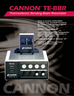


© Copyright 2026