1. technology and computing
2. software
3. databases

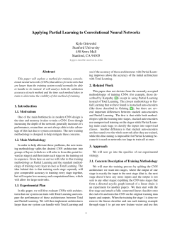
Geo-Location Estimation with Convolutional Neural Networks
Amani V. Peddada
James Hong
[email protected]
[email protected]
Abstract
2. Related Work
There have been several approaches in the past that have
focused on various levels of geo-location estimation. Zamir and Shah, in [2], propose a novel variant of the Nearest Neighbor algorithm using Generalized Minimum Clique
Graphs (GMCPs) to exceed state-of-the-art results in geolocalization. This initiative built upon their previous work
of matching using SIFT features and trees [1], to perform
fine-grained localization within cities.
The research conducted by Jones in [8] makes use of
both hierarchical classification and dictionary-based recognition to categorize images into a set of cities or landmarks
within the United States. Schindler et al. [4] perform exact geo-placement within a single city using a vocabulary
tree to efficiently search a database of street images that
might be proximal to query images. Hays and Efros utilized a dataset of 6-million geo-tagged images from Flickr,
and performed classification on multiple granular scales to
obtain reasonable performances on a dataset that was more
ambiguous due to noise present in the labels [6].
There has also been a substantial amount of research
conducted on the closely related challenge of scene recognition. In particular, Zhou et al., obtained state-of-the-art accuracies by applying CNNs to Places, a database consisting
of over 7 million labeled images of scenes [9]. Likewise,
MIT’s Scene Understanding (SUN) database has been the
subject of much research in scene recognition, where feature extraction methods combined with standard machine
learning techniques have produced optimal performances in
determining from a choice of 908 scene categories [5].
However, to the best of our knowledge, there have been
no approaches that have made significant use of Convolutional Neural Networks (CNNs) for the task of geolocalization. Given the rapidly increasing usage of deep
learning in all varieties of recognition problems, we believe
that CNNs will in fact be inherently suited to this task, and
that the networks will be able to extract the fine details and
similarities that are associated with specific localities. We
therefore construct and tune several CNNs to classify images according to discretized geo-locations, and then conduct a rigorous evaluation of the performance of our models.
We explore the extraction of geo-spatial information
from purely visual data. Though there have been previous
attempts to apply machine learning and computational algorithms to this fundamentally subtle task, to the best of our
knowledge, there are no initiatives that have directly utilized
Convolutional Neural Networks (CNNs) for the challenge
of geo-localization. This project thus employs a methodology that explores CNNs in conjunction with an investigation
of existing computer vision techniques to analyze images
according to their geospatial attributes. We apply CNNs
to coarse and fine grained image classification on Google
Street View data to predict city and location within a city, respectively. We also apply our models to location-tag prediction on a diverse dataset of images from Flickr. Our results
demonstrate that our trained CNNs excel at both coarse
and fine classification tasks and approach near human accuracy levels for location tag prediction when applied to
noisy, real-world, datasets.
1. Introduction
The idea of estimating “geo-location” is an inherently
rich and yet remarkably unexplored subject. It remains a
topic unlike many others in the standard domain of computer vision or recognition since it requires the identification of more key, abstract features that remain constant
across large spatial and temporal scales – making it an inherently subtle yet novel task. It also represents an integral
part of the human experience, where we ourselves possess
the innate ability to extract contextual information from the
environment in order to draw conclusions about our current location and surroundings. Understanding and achieving visual geo-recognition is therefore crucial towards the
development of a more refined and sensitive Artificial Intelligence framework.
In this project, we thus evaluate fine-tuned techniques
for extracting geo-spatial information from image data. We
propose one of the first applications of Convolutional Neural Networks to this task, and obtain superlative results on
classifications at various granularities.
1
3. Technical Approach
• One-V-All Support Vector Machine (SVM) We
build a single binary, max-margin SVM for each class
that determines whether a given image belongs to that
class or not. During testing, we then see which SVM
outputs the greatest score for that example, and choose
the corresponding label as our prediction. We experiment with linear, Gaussian, and polynomial Kernels.
We now formulate the challenge of visual georecognition as follows: Given images captured from a variety of localities around the world, how closely we can create
a correspondence between these images and their original
locations?
To work towards this goal, we divide our task into two
distinct classification problems:
• Artificial Neural Network (ANN) We construct a
standard feed-forward, back-propagating neural network, with four hidden layers containing 400, 250,
100, 50 nodes, respectively.
• Coarse Classification - Given a testing image, determine the corresponding city in which the image was
captured.
• Convolutional Neural Network (CNN) We train
models both from scratch and with transfer learning.
We also perform basic data augmentation by flipping
images and oversampling crop areas. All of our training and validation images are down-sampled to dimensions 256x256x3. We obtained the best results using
the following architectures:
• Fine-Grained Classification - Given an image taken
from a single city, predict the exact, corresponding
sub-region within the city.
To approach these two challenges, we train and evaluate our models on a dataset of Google Street View images
obtained by Zamir and Shah in [2]. The dataset itself contains a total of over 62,238 RGB images taken from 3 cities:
Pittsburgh, New York City, and Orlando. For each city,
a set of images is captured at placemarks located roughly
12m apart, allowing for more fine recognition than would
be possible for datasets of less uniformly or less densely
scattered data. Each placemark contains a total of 5 images, representing four panoramic side views and one upward view. Within this dataset, there are approximately
5500 placemarks from New York, 3000 from Pittsburgh,
and 1500 from Orlando. Each image is labeled with GPS
and compass coordinates, and all were taken in outdoor environments under similar physical conditions.
However, since the Street View images follow a fairly
consistent structure, we also perform experimentation with
a more challenging classification problem by utilizing
Flickr’s diverse 100m image dataset in order to measure the
generalization capabilities of our models [3]. Each image is
mapped to associated meta-data, such as user/machine tags,
and 49m of the photos are geo-tagged with latitude and longitude coordinates.
We then evaluate our models on these datasets using
CNNs and several baseline algorithms for comparison:
1. CNN (from scratch) We used the (conv-relupool)x3-affine architecture. Each conv layer used
5x5 filters, 2 pixel padding, and stride 1. The
number of filters at each level were 32, 64, 64 for
levels 1, 2, and 3. The pooling layers are maxpool with stride 2 and 3x3 areas.
2. NIN-Imagenet Transfer Learning In order to
facilitate faster training and better performance,
we used the NIN-Imagenet model [7], retraining
the final convolution layer and adding a fully connected layer. We further experimented with addition of convolution and fully connected layers,
but validation performance remained roughly the
same, despite much longer training times.
In sections 4 and 5, we discuss the details of Coarse and
Fine-Grained Classification, respectively, and in section 6
we describe the results of the Flickr experiments.
4. Coarse Classification
We here describe our experiments with coarse classification, in which we seek to categorize images according to
different cities.
• Feature Extraction We first implement feature extraction techniques to serve as input for our baseline methods. We experiment with both 60-dimensional Color
Histogram features, and 960-dimensional GIST features.
4.1. Experimental Setup
Using the Street View dataset, we randomly sampled
4400 images each from Pittsburgh, New York City, and Orlando to serve as a training set for our algorithms, and likewise extracted 800 each for our testing set. We ran all of
our baselines on Color Histogram features (the addition of
GIST showed little improvement), and trained two CNNs
on the raw input images: one from scratch, and one with
• K-Nearest-Neighbors We apply the K-NearestNeighbor algorithm to our data as a simple baseline.
This involves simply finding images in our training set
that are closest in distance to the features of our testing images, where we used Euclidean distance as our
metric. We cross-validate to find optimal values of k.
2
the Network-in-Network structure. Sample images and results are shown below. (Note: We also tested ensembled
CNNs by averaging scores across 10 unique models, but
the gains were insignificant (< 0.5%) at the cost of being
highly time-consuming to train.)
KNN performs surprisingly well given its simplicity; this
makes sense, for the task of geo-location as we have formulated it lends itself nicely to the properties of KNN. We can
see there are a number of factors in the Street View dataset
itself that might lead to this high performance. For example,
since each placemark is located approximately 12m apart
from the next, we have sets of images that are very similar to each other, so every photo has an assortment of extremely close yet valid neighbors. We would expect KNN
to perform less optimally, if the photos were densely and
uniformly distributed across the city, had dissimilar viewpoints/angles, or if we extended our classification to more
city subsections or larger numbers of cities.
Our one-v-all SVM, interestingly, does not perform as
well as KNN. Using a linear or polynomial Kernel obtains
accuracies only slightly greater than chance (33%). Using
a Gaussian radial basis function gives approximately 57%,
but even this is still significantly below the performance of
KNN, indicating that SVMs may not simply be suited to
this type of task. It would be interesting to experiment with
other varieties of the multiclass SVM or other Kernels to
see if they obtain similar performances.
However, though our standard Neural Network seems
to produce the best testing accuracy of the baselines, our
CNN trained from scratch by far outperforms all baseline
methods by a considerable margin – we expect this is simply because the network can capture a much richer amount
of detail and abstraction from the images than the baseline
methods. The CNN trained using transfer learning from
the Network-In-Network model, however, seems to output
a lower accuracy – but this follows intuition, since we keep
the early layers of the pre-trained network fixed, and only
re-train the last layer appropriately, making it more difficult
to adjust flexibly to the structure of our data in a simple 3way classification problem.
Figure 1. Images from Street View dataset [2].
4.2. Results
We display the results of our experiments below
k
GIST
CH
1
51.3
66.2
4
52.1
67.3
5
51.0
67.1
7
50.3
66.6
10
51.0
66.7
15
49.6
66.1
20
49.7
64.7
Table 1. Accuracy of KNN for varying k on GIST and Color Histogram features. k = 4 is optimal
Model
KNN (k=4)
SVM
ANN
CNN
CNN-Transfer
Accuracy
67.3
56.1
68.5
97.5
86.0
Table 2. Accuracy of coarse classification models. KNN, SVM,
ANN were run on CH with optimal parameters.
Class
Pittsburgh
Orlando
New York City
Recall
98.6
99.5
93.5
Precision
94.9
97.4
99.5
Table 3. Classification precision and recall by class for CNN
trained from scratch.
4.3. Evaluation
Figure 2. Visualization of first conv layer weights for CNN trained
from scratch.
As we can see, of the baseline algorithms, both KNN
and the ANN perform reasonably well in this classification
problem while our ConvNet trained from scratch achieves a
near perfect accuracy of 97.5%.
3
Figure 5. Images falsely classified as NYC; all are very urban.
(Pittsburgh, Pittsburgh, Orlando, Pittsburgh)
Figure 3. Visualization of second conv layer weights for CNN
trained from scratch.
Figure 6. Images falsely classified as Orlando; note the large presence of vegetation. (Pittsburgh, Pittsburgh, Pittsburgh, NYC)
Figure 4. Visualization of third conv layer weights for CNN trained
from scratch.
Upon visualizing the conv-layer weights of our CNN
(see above), we notice that many of the filters in the first
layer capture strong color information – perhaps corresponding to how lush a particular city is, the general hues
of its buildings, or the weather in the sky. Indeed, this
might also be indicative as to why color histograms produce optimal results for our baseline measures. Additionally, there are some textures that seem to represent building edges/architectures, or perhaps some street boundaries.
However, in the higher levels of the network, we do not notice necessarily distinct shapes in the weights as we would
in standard object recognition tasks – this is expected, since
the ConvNet is extracting broader trends for the more general task of geo-recognition, where there are no single objects in view and instead more varied backgrounds.
One interesting fact is that most of the mis-classifications
of the ConvNet were between New York City and Pittsburgh, and Orlando was not as often mistaken – thus the
CNN had little trouble detecting the more distinctive atmosphere of Orlando; Pittsburgh and NYC on the other hand
are arguably much closer to each other in terms of environmental/physical conditions (both in urban settings).
It should also be noted that our dataset is limited since all
of the photos were captured under similar illumination and
outdoor conditions. We could likely make our CNN more
robust with the inclusion of images taken from various times
of the day and under different viewpoints or angles.
Figure 7. Images falsely classified as Pittsburgh; like NYC, the
images are urban but less dense. (NYC, NYC, NYC, NYC)
5. Fine-Grained Classification
In this section, we discuss our experiments with finegrained classification within a single city.
5.1. Experimental Setup
We investigate performance by predicting sub-regions
specifically within New York City, which was chosen due to
its dense distribution of data-points. The Street View dataset
contains 23,762 NYC images in total, which we partition
into 21,762 and 2,000 for train and test, respectively. Note
that we first divide the dataset before defining fine location
classes in order to maintain consistency and comparability
between our experiments at varying degrees of fineness.
We developed two strategies for defining fine location
classes: tiling by latitude/longitude and recursive subdivision. In tiling, we create a grid whose components are of
equal spatial size; however, because the images are not uniformly distributed across the city, tiling often yields buckets that are unbalanced in their number of constituent data
points. Recursively subdividing until reaching a maximum
bucket size solves this problem, but makes less sense from
a semantic perspective, since we begin to classify between
bins of inhomogeneous dimensions – we therefore decide
to use the tiling approach in all of our experiments. To account for the possible unbalanced distribution of data points
within our buckets, we devise a sum/mean error distance
4
metric in addition to obtaining raw accuracy to evaluate our
methods.
5.1.1
files). This allowed us to train more CNNs and experiment
with larger ranges of granularities.
5.2. Results
Distance Metric
5.2.1
We evaluate mean distance using the following formula. For
the predicted geolocation, we use the center of the tile corresponding to the predicted label. The true geolocation is
the exact latitiude/longitude of the image, prior to tiling and
partitioning. This limits the minimum possible error achievable for larger granularity (even 100% raw accuracy will
result in a non-zero error). However, by comparing predicted geolocation against true geolocation as opposed to
mean geolocation of tiles, we allow for meaningful distance
comparisons for different granularites of classification.
Model
train
val
Thousandths of a degree (lat/lon)
100
50
20
10
5
85.8 78.2 68.5 68.9 52.7
85.0 74.1 67.1 60.9 48.1
1
68.5
43.3
Table 5. Accuracy on train and validation sets vs. fineness of class
labels for CNN.
Model
KNN
ANN
CNN
1 X
D(Geolocation(yim,pred ), Geolocation(yim ))
n
im∈X
Thousandths of a degree (lat/lon)
100
50
20
10
5
83.0 68.6 59.3 50.0 43.5
74.8 49.9 39.5 22.8 9.10
85.0 74.1 67.1 60.9 48.1
1
30.5
0.20
43.3
Table 6. Validation accuracy for KNN, ANN, and CNN compared.
Note that the labels are represented as latitute, longitude
pairs. We use the Haversine formula to compute distance
between points.
5.2.2
5.1.2
With Raw Accuracy
With Distance Metric
Tiling & Partitioning
Model
KNN
CNN
Thousandths of a degree (lat/lon)
100
50
20
10
5
3.81 2.78 1.80 1.40 1.28
3.76 2.63 1.35 1.06 1.05
1
1.23
0.78
Table 7. Mean euclidean distance error on validation sets vs. fineness of class labels for KNN and CNN.
Figure 8. Visual comparison of tiling (left) and recursive (right)
partition strategies.
Deg
0.1
0.05
0.02
0.01
0.005
0.001
# Tiles
3
5
14
31
79
734
W (km)
9.6
4.83
1.931
0.960
0.483
0.096
H (km)
11.100
5.550
2.220
1.110
0.555
0.111
Area (kmˆ2)
107.200
26.800
4.290
1.070
0.268
0.011
Figure 9. Histogram of euclidean distance errors on validation for
0.001 degree bins/734 way fine-grained CNN.
Table 4. Tile size in degrees (lat/lon) vs. number of tiles and dimensions.
5.3. Evaluation
We trained our CNN models for each granularity using the NIN-Imagenet model, which was selected due to
its solid performance on ImageNet classification (slightly
better than AlexNet) and relatively small number of parameters (only 30.4MB compared to 411.6MB for VGG model
As with coarse classification, we see that KNN with
color histogram features performed quite well, but this is
once again likely due to the overlapping/telescoping structure of the Street View dataset. By cross-validating over the
5
6.1. Initial Experiments
data, we find that KNN performs optimally at k = 1, and,
in general, performs noticeably less well with larger values
of k. One cause of this behavior is that as bins become too
small, there will be fewer neighbors in the correct bin, and
larger numbers in nearby incorrect bins, so using larger values of k introduces the potential for error in our estimates.
We initially identified 50 cities from around the world
and proceeded to filter the 100m Flickr images based on
geo-coordinates. However, we quickly found this approach to be impractical due to the quality of the coordinate
tags, which were not correlated with outdoor or locationrelevant images. For instance, we found hundreds of images
from Bakersfield, CA of poorly lit indoor concerts, hockey
matches, and family portraits.
Subsequently, we re-sampled images from 50 locations
based of subject tags rather than coordinate tags, where we
used the most popular subject tags based on Flickr’s page.
We further filtered the candidate set of images by popular
tags including ”architecture”, ”city”, ”landscape”, ”urban.”
This yielded a slightly cleaner dataset, with some quirks
such as a few classes corresponding to city names, and others to countries (e.g ’london’, ’germany’. ’scotland’). Another challenge was that many classes in the dataset were
extremely similar; for instance, there was not enough distinction between images from ’shanghai’ and ’beijing’ in
order for a classifier to make meaningful predictions. Unfortunately, these challenges led to poor CNN performance
on this initial dataset ( 4% – only 2x better than chance).
Compared with KNN and CNN, the ANN model falls
off very quickly in accuracy, which is somewhat interesting
given its reasonable performance on coarse classification –
but this might be due to the more complex input space that it
is attempting to model, since nearby buckets presumably are
quite similar to each other and have ambiguous boundaries
that are more difficult to take into account.
Our CNN with transfer learning, however, performed optimally over all methods in terms of both the raw accuracy
and distance metrics. Comparing our training and validation accuracies for our CNN, we notice that the values tend
to closely approximate each other at each granularity level.
The low generalization error suggests that the CNN lacks
the model capacity to obtain higher classification accuracy.
This lack of overfitting is once again perhaps due to the
large similarities between adjacent tiles and the contrived
boundaries enforced by tiling. A more clever scheme for
determining bucket boundaries might mitigate this issue.
Additionally, as the bins become smaller, we might have
too few points in many categories to affect the CNN in significant ways, so having more data in each category could
perhaps improve performance.
6.2. Experimental Setup
We redefined the problem in response to the challenges
from our initial experiments, selecting 10 locations from
the previous 50 popular subject tags. We chose these locations by tag popularity and by uniqueness to measure the
CNN’s ability to capture context cues about the location.
For each tag we sampled 2,500 images; due to irregularities
with Flickr links and tags (as well as ’newzealand’ being
smaller than the other classes), this yielded a final dataset
of 23,321 images, of which 2000 were set aside for validation (100 per class).
Overall, our results demonstrate that raw accuracy decreases as the size of the tiles decreases (or as the number of tiles increases) – this makes sense, because our output space is growing while the number of datapoints per
class decreases. However, performance relative to chance
improves significantly as the fineness is increased for both
CNN and KNN – for 734 bins, for example, we obtain over
43% accuracy with our CNN. Performance on the distance
metric paints a similar picture, where with finer-classes, the
mean error drops significantly. At 0.001 degree lat/lon granularity (734 classes) the distribution of error is highly Zipfian, indicating that, even in cases of misclassification, the
assigned tile is likely close to the actual tile. These results
suggest that, in the CNN case, our learned model is able to
capture location specific information such as architecture,
plants, etc of the tiles.
Figure 10. Location labels for 10-way Flickr classification task.
6. Flickr Dataset
We tested both a 4-layer CNN from scratch as well as
performed transfer learning with the NIN-Imagenet model
with all but a final fully connected layer fixed. We also manually labelled 100 images to provide a baseline for human
performance.
We extend our goal of geo-localization to real world conditions to predict user generated location subject tags for
Flickr images; we thus present a more challenging task on
a much more noisy dataset.
6
6.3. Results
6.4.2
Model
CNN
CNN-Transfer
Human
Train
32.47
43.40
-
Classifying these images is difficult, even for a human. Like
the CNN, our labelling efforts were confounded by noise
in the dataset. We were able to perform slightly above
the CNN accuracy using prior knowledge (e.g. recognizing Portugese on Brazilian signs, scenes from Death Valley,
penguins from New Zealand, etc.). Below are some examples of correctly/incorrectly classified images.
Val
29.21
38.55
42.00
Table 8. Comparison of CNN model performance and human accuracy on 10 way Flickr image classification.
Class
Dubai
Venice
New Zealand
Turkey
Paris
Russia
India
Brazil
USA
China
Recall
62.0
60.5
37.0
36.0
35.5
34.0
31.5
31.0
31.0
29.0
Human Performance
Precision
41.8
42.3
67.9
43.9
40.1
46.9
30.8
35.0
21.7
34.6
Figure 13. Images that were classified correctly by humans.
Table 9. CNN-NIN-Imagenet-transfer precision and recall breakdown by location class.
Figure 14. Images that were misclassified by humans.
6.4. Evaluation
6.4.3
6.4.1
Both the CNN and the human classifiers picked up general patterns in the data. This is reflected in the high variance in precision and recall percentages for each class label. For instance, the CNN learned to associate water in the
foreground with Venice, and landscape images with New
Zealand. Interestingly, the CNN also learned to classify
high-key images as Russia, possibly due to a large number of images containing snow. It was also able to capture
architectural styles and tourist landmarks for Russia, India,
China and Paris.
CNN Performance
The CNN trained from scratch performed much worse than
the CNN with transfer learning with the NIN-Imagenet
model. Some possibile reasons are: first, for tractability
the CNN from scratch is much smaller than NIN-Imagenet,
and second, NIN-Imagenet model works well as a feature
extractor for the Flickr classification. As with fine grained
Street View classification, generalization error is relatively
low. Because the models were trained till convergence, we
conclude that this is due to the hard, noisy properties of the
dataset.
Error & Pattern Analysis
Figure 15. Images that were incorrectly classified as New Zealand.
(Russia, Brazil, Turkey, Turkey)
Figure 11. Images that were classified correctly by the CNN.
Figure 16. Images that were correctly classified as Russia; note the
presence of landmarks and Eastern Orthodox church architecture.
Figure 12. Images that were misclassified by the CNN.
7
• Model tuning For transfer learning, we could train
more layers to obtain a model more suited to our
geo-localization task. This would likely require more
time and GPU processing power than available to us
currently. Where appropriate for larger classification
problems, we would use a more capacitive model,
adding more receptive fields, layers, etc.
Figure 17. Images that were correctly classified as China.
• Generalizing to more test data We can test our Street
View models on landscape urban images from other
sources such as Flickr, Facebook, etc. to determine
how finely we can localize these new images. However, generalizing the Street View images to these
other mediums requires a non-trivial amount of preprocessing.
Figure 18. Images from USA that were incorrectly classified.
(Dubai, Dubai, New Zealand, Paris)
We see that many of the errors produced by the CNN are
reasonable, at least to the extent that a human would make
the same errors.
6.4.4
• Hierarchical classification We could ensemble our
classifiers at different granularities to build a heirarchical model that allows us to accurately perform fine
classification across several cities. This would truly
test the CNNs ability to generalize to useful real world
scenarios and would reveal much information as to the
inherent structure of our data.
Dataset Quirks/Noise
The difficulty of the Flickr classification problem is compounded by the noisiness of the labels. Flickr users have
very different standards when it comes to labeling their images. For example, one user might tag the Eiffel Tower as
architecture, while another might tag a brick wall or the
pavement. We found that a single user in Taiwan labeled
many flower images as landscapes. In addition, many of the
supposed architecture images were ’selfies’. Finally, some
images in the dataset are flatly mislabeled (e.g. we found
a picture of the Eiffel Tower labeled as Brazil). Thus, it
is remarkable the CNN still managed to achieve reasonable
performance despite this large amount of noise.
• Additional Flickr data We can improve the 10-class
Flickr dataset by adding more classes and applying
stronger filters to surpress noise, especially in less
common tags.
In any case, we still believe that the use of CNNs in geolocalization is still a tremendously unexplored area, deserving of further investigation.
8. Conclusion
In this report, we have presented several approaches for
addressing the challenge of geo-location estimation. In particular, we have shown the first application of CNNs to this
task, and have demonstrated that they can obtain superlative
performance on both coarse and fine-grained classification.
Finally, we have substantiated CNN’s ability to generalize
to geo-localization of more varied forms of data (Flickr),
approaching near human accuracy.
Figure 19. Left: the Petronas Towers tagged as Dubai. Center: the
Eiffel Tower tagged as Brazil. Right: an Arc de Triumph lookalike in the USA. For these images the CNN predicted, reasonably,
Dubai, Paris and Paris.
9. Acknowledgements
We would like to acknowledge Amir R. Zamir, Ph.D. for
his help and guidance in obtaining the Street View data.
References
7. Future Directions
[1] A. R. Zamir and M. Shah. Accurate Image Localization Based
on Google Maps Street View. Proceedings of the 11th European conference on Computer vision, 2014.
[2] A. R. Zamir and M. Shah. Image Geo-localization based on
Multiple Nearest Neighbor Feature Matching using Generalized Graphs. IEEE Transactions on Pattern Analysis and Machine Intelligence (TPAMI), 2014.
Our results demonstrate that we can obtain very reasonable performance predicting geo-location from purely image data using CNNs. We also believe that there is room
for further improvement. Some possible ways to extend
this project to obtain even better results or error analysis
include:
8
[3] D. A. Shamma. One hundred million creative commons flickr
images for research. 2014.
[4] G. Schindler, M. Brown, and R. Szeliski. City-scale location
recognition. Proc. IEEE Conf. Computer Vision and Pattern
Recognition, 2007.
[5] J. Xiao, J. Hays, K. Ehinger, A. Oliva, and A. Torralba. Sun
database: Large-scale scene recognition from abbey to zoo.
2010.
[6] James Hays, Alexei A. Efros. Im2gps: Estimating geographic
information from a single image. 2009.
[7] M. Lin, Q. Chen, S. Yan. Network in network. International
Conference on Learning Representations, 2014.
[8] M. W. Jones. Image geolocation through hierarchical classifcation and dictionary-based recognition. 2012.
[9] B. Zhou, A. Lapedriza, J. Xiao, A. Torralba, and A. Oliva.
Learning Deep Features for Scene Recognition using Places
Database. NIPS, 2014.
9