Download Report

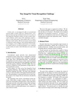
Tiny ImageNet Challenge Submission
Lucas Hansen
Stanford University
[email protected]
Abstract
order to prevent over-fitting to the test dataset.
The current state-of-the-art on the ILSVRC dataset is a
top-1 accuracy rate of 23% [1] using a very deep convolutional neural networ. The Tiny ImageNet challenge is a
strictly simpler version of this problem, so ideally it should
be possible to get an even better top-1 accuracy than 23%.
However, there is the caveat that each image has been downsampled to 64x64 pixels (normally the images are much
larger in ILSVRC), and upon further investigation it seems
that this has significantly impacted performance.
The problems caused by downsampling all of the images to 64x64 pixels are more subtle than one might expect.
Figure 1 shows some example images from the Tiny ImageNet dataset that have been severely effected by the downsampling. The average image size in the vanilla ImageNet
dataset is 482x418 pixels with an average object scale of
17.0% [3]. This means that to downsample the image to
64x64 pixels we must first throw away 13.3% of the image (to make it square), and then shrink it by a factor 6.5,
on average. This transformation has 4 potential negatives
consequences on the image:
Implemented a deep convolutional neural network on the
GPU using Caffe and Amazon Web Services (AWS). Current
architecture is based on AlexNet augmented with Parametric ReLU’s. Preliminary results show a classification accuracy of 45% on the validation set.
1. Introduction
The goal of this project is to build an extremely accurate classifier for the Tiny ImageNet dataset. This dataset is
a strict subset of the ILSVRC dataset (containing only 200
categories rather than the usual 1000 categories). In general, we would expect that the same sorts of techniques that
work well on the ILSVRC dataset would also work well on
the Tiny ImageNet dataset, so much of this project will be
applying techniques which were successful on ILSVRC in
recent years.
At this scale of problem it is imperative that we use a
GPU as our primary computation device so that we can
rapidly iterate and cross-validate designs. So this project
will focus on designs that have already been optimized to
run quickly on the GPU.
(a) Scaling artifacts are introduced
(b) The object of interest is cropped out
(c) The object of interest is tiny
2. Tiny ImageNet Challenge
(d) Much of the texture in the image is lost or distorted
The Tiny ImageNet dataset is a strict subset of the
ILSVRC2014 dataset with 200 categories (instead of 100
categories). Each class has 500 training images, 50 validation images, and 50 testing images. Each image has been
downsampled to 64x64 pixels. The testing images are unlabeled and bounding boxes are provided for the training and
validation images only. The accuracy of a classifier is defined as the percent of the test images which are correctly
classified. Naturally the accuracy of a classifier cannot be
measured directly by any of the participants in this challenge. A participant must upload labels for all of the test
images produced by his classifier, and an evaluation server
then scores this labeling and updates the live scoreboard.
New submissions are only accepted once every 2 hours in
It is not clear exactly what effect (a) has on performance.
As long as the model is trained from scratch it may not effect anything. In fact, since the scaling artifacts are dependent on the properties of the original image, it may actually
help in classification by providing additional global information. However, it would likely be quite detrimental in
a model that relies on fine-tuning an existing CNN. Both
(b) and (c) are similar in nature; the object of interest is either not present in the image or its representation is much
reduced. This can be a major issue for object categories
that lack distinctive background imagery, but as discussed
in [4] for many categories the background imagery is sufficient for accurate classification. In these cases, (b) and
1
(a) Orangutang
(b) Broom
(c) Popsicle
(d) Trolleybus
(e) iPod
(f) Lighthouse
(g) Bikini
(h) Lawnmower
Figure 1: Some examples of difficult images. Note the scaling artifacts prominent in (a) and (d), the loss of texture in (c) and
(g), the loss of crucial information due to cropping in (b), (f), and (h), and the difficulty of locating small objects in (c).
to work better and that a network should be be made as deep
as possible while still being trainable.
There have been a few particularly novel and useful contributions that have been over the past few months that
we would like to integrate into our approach. The first of
these, the so called ”Inception module” [2] or ”NetworkIn-Network” structure [7], was a part of the GoogLeNet
which won ILSVRC this year. The basic idea is to build
a convolutional neural network out of components which
are more complicated than a single convolutional layer. In
GoogLeNet the basic component combines 4 parallel convolutional layers with different filter sizes. Google claims
that this model was behind their incredible performance at
ILSVRC 2014. The second idea is the idea of a Parametric
ReLU (PReLu) [1]. A PReLU is essentially a leaky ReLU
whose degree of leakiness is trained during backpropogation rather than set by cross-validation. It introduces very
little performance overhead, but for many use cases is able
to significantly boost classification accuracy. The third idea
is a strategy for reducing internal covariate shift between
layers using a technique called Batch Normalization, explored in [8]. This technique yielded incredible improvements in both training accuracy and, most dramatically, in
training speed. The authors of the paper claim that for a
wide variety of networks, training time decreased by a factor of 10-15x.
Where possible we did our best to use these breakthroughs in our classifier. Unfortunately, since many of
(c) may not be much of an issue. Perhaps the most significant distortion introduced by the image transformation
is (d). In [4], Russakovsky et al. show that CNN’s sometimes rely more heavily upon local texture information than
global information for classification. Image rescaling introduces pseudo-random distortion onto most of the textures
in the image, and hence is probably responsible for why the
Tiny ImageNet Challenge isn’t strictly easier than ILSVRC.
Unfortunately, none of these issues are easily remedied by
post-processing.
3. Related Work
The ImageNet ILSVRC has been run every year for the
past four years, producing hundreds of different models for
the various different competition categories. Since our approach is so heavily inspired by ILSVRC submissions from
recent years it is useful to review some trends in the winners
from the past few years.
Not surprisingly, the most persistent trend in recent years
has been towards deeper and deeper convolutional neural
networks. This began with Krizhevsky et al. in [5], and
every year since then has seen more and more varied submissions using convolutional neural networks. Most recently, in ILSVRC 2014 GoogLeNet [2] and VGG [6] performed extremely well in the object recognition and localization categories, respectively. Some lessons learned from
these papers are that smaller convolutional filter sizes tend
2
Figure 2: A diagram of our most performant network architecture. The gray ovals are blobs, Caffe’s terminology for chunks of memory used throughout the
forward pass.
these techniques are so new, there sometimes wasn’t a reliable open-source implementation, which limited our ability
to explore their usefulness.
4. Technical Approach
There are two main prongs to our approach. The first is
architecture and the second is the technical details of training that architecture. We will discuss the architecture of the
CNN first and the details of training afterwards.
4.1. Architecture
We are using Caffe to model and train all of our networks and so it is very important that we choose architectures that are simple to implement on this platform. As an
initial baseline we just slightly modified Caffe’s implementation of AlexNet to run on the Tiny ImageNet dataset (we
just changed the crop size to 60 to deal with the fact that our
images are only 64 by 64 pixels). This network has 5 convolutional layers, 3 max-pool layers, and 3 fully connected
layers. By default the Caffe implementation of AlexNet
uses only random crops and mirroring for data augmentation. This produced a top-1 accuracy of 25%. Very little
hyper-parameter tweaking was required, as AlexNet came
with a default set of hyper-parameters known to work very
well for that network. The default AlexNet implementation
trained much, much faster than any of the other models that
we tried.
Since then we have made a few more modifications
based off of the advice that we have been given in lecture.
We removed the normalization layers, decreased the size of
the max-pool kernel, and changed most of the filter sizes to
3. This resulted in an increase in performance of roughly
10%, bringing us to a top-1 accuracy of 35%. Although
these changes resulted in a net increase in performance, we
needed to perform quite a lot of hyper-parameter search to
get the network to train properly. Some of the most important modifications involved changing the base learning
rate and learning rate annealing schedule. We observed that
the default settings of AlexNet make very inefficient use
of GPU time. The default strategy is a base learning rate
of .01 and annealing the learning rate by 10 every 100000
iterations. We noticed that the network converged much
more quickly when we annealed by 10 every 5000 iterations instead of every 100000 iterations. For the final model
we manually slowed down the annealing schedule to get
the best possible performance but during development and
cross-validation such slow convergence is not practical.
After these basic modification, we found that it was very
difficult to increase the performance of the network. We
experimented with adding and removing pooling layers,
adding and removing convolutional layers, changing the
number of neurons in the fully connected layers, changing
the number of fully connected layers, experimenting with
3
from UC Berkeley. This is a relatively expensive way of
doing things but there doesn’t really seem to be a viable alternative. All told, we probably ended spending somewhere
on the order of $125 on EC2. This is much cheaper than
purchasing a computer with a capable graphics card, but it is
still a non-negligble cost. To be honest, given how much we
learned from this project, the cost seems more than worth it.
Because the Tiny ImageNet dataset has many fewer images than ILSVRC and all of the images are downsampled
to 64 by 64 pixels, all of the data is able to easily fit on the
GPU. So the 4GB GPU available on the Amazon G2 EC2
instances is sufficient.
We trained the final model depicted in 2 for about 1.5
days, occasionally manually tweaking the learning rate so
that network never got stuck in local optima.
Figure 3: ReLU vs PReLU. For PReLU, the coefficient of
the negative part is not constant and is adaptively learned.
This plot and caption are originally from [1]
different training schemes (including SGD, AdaGrad, and
Nesterov’s Accelerated Gradient), and nothing really improved the performance of the network (although Nesterov
was able to speed up training by approximately a factor of
2). In particular, varying the number of layers in the network was pretty disastrous. When removed any of the layers, the performance was extremely poor and whenever we
added a new layer the network was unable to converge. This
was probably due to improper hyper-parameter settings, but
cross-validation to find better parameters is extremely computationally expensive.
We also tried ensemble techniques, although the number of classifiers in the ensemble was generally quite small
(between 2 and 4 models) due to our limited computational
budget. The ensemble was created by simply averaging the
activations of the last layer of every network, and takign
the max activation of the averaged model to be the category
prediction. Unfortunately, at least with the small number of
models that we tested out, ensembling yielded no increase
in classification accuracy, and in fact very slightly decreased
test set performance.
There was one final adjustment that yielded a surprisingly sizeable increase in performance for very little work.
We replaced all of the ReLU’s in our network with PReLU’s
[1]. This single change yielded an almost 10% increase in
performance. As [1] suggests, we used Xavier weight initialization, and although we were not able to exactly replicate their weight initialization methods, using Xavier did
seem to speed up the training process. Figure 3 shows how
the activation function in a PReLU works. Our final submission used PReLU’s together with architecture shown in
Figure 2.
5. Results
Using the network depicted in 2 we were able to achieve
a top-1 accuracy of 45%. When we started the project, and
after the first milestone, we hoped that we would be able to
do much, much better than this, but unfortunately the problem turned out to be harder than we thought. We suspect
that this is partly because of our inexperience at choosing
the hyper-parameters for extremely large CNN’s, but also
partly because of the distortion introduced into the image
by scaling.
6. Future Work
There are still many, many things left to try. For instance,
we should probably try more types of data augmentation.
As we learned in Assignment 3 contrast and hue data augmentations and can significantly help the performance of
a CNN, especially when there is not a ton of data. And
of course the default AlexNet is not particularly deep compared to more modern architectures and it could be fruitful
to try architectures with many more convolutional layers.
We very much wanted to try out Batch Normalization
as described in [8], since the reported increase in performance would have drastically sped up training and crossvalidation. Given our limited computational budget, a 10x
speedup in training time would’ve allowed us to try out
vastly more models, and would’ve made architectures that
were infeasible for us to train from scratch, such as VGG
[6], possible to experiment with. Unfortunately, this technique is extremely new and not trivial to implement. So at
the moment no working implementation exists in Caffe.
In our original proposal we said that we were interested in implementing Google’s Inception CNN (which won
ILSVRC 2014) for the GPU, because so far it had only
been implemented for the CPU. It turns out that although
Inception has only been implemented on the CPU, it was
actually run on an enormous cluster of computers, specially
4.2. Training
As we have mentioned earlier, all of the training for
our network was performed with Caffe on a GPU. Unfortunately, we do not have access to our own personal GPU.
So we have been running all of our training on a G2 Amazon EC2 instance, using an AMI prepared by Achal Dave
4
(a) Raw Image
(b) First Layer Weights
(c) Filtered Image
(d) Second Layer Weights
Figure 4: Visualization of some early network layers
designed by a research group at Google for training Convolutional Neural Networks. And the network architecture
was designed to take advantage of the particular properties
of this computer cluster. So it is unlikely that implementing
Inception on a GPU would render any real performance improvement. On a sidenote, as of early January, Caffe now
comes with an implementation of Inception by default.
The thing that we are most eager to try is running our
models on the full-sized images. We suspect that we would
have greatly increased performance on the raw dataset, and
that since there are fewer categories in the Tiny ImageNet
Challenge than ILSVRC, we might be able to have a better
top-1 accuracy than that reported in the ILSVRC submissions.
lenged the ILSVRC, which has so greatly influenced the
growth of computer vision over the past few years. In any
case, this competition was sufficiently involved that I feel
fully capable of working on a CNN centered independent
project in the future. And given how incredible the perfomance of these models are, I have little doubt that I will take
advantage of this knowledge before long.
Thanks to Andrej, Fei-Fei, and the TA’s for putting on
such an incredible class! It is certainly one of my favorites
at Stanford. I had more ”wow” moments in this class than
any other class that I have ever taken. Before this class I
didn’t have too much interest in computer vision, but that
has now changed drastically. For the sake of all Stanford
students, I hope that this class is taught again next year!
7. Conclusion
References
This was an extremely rewarding project. We learned
a lot of things in this class about convolutional neural networks, and all of the assignments contained lots of hands-on
examples, but it still felt like a very structured environment.
Until this project I wasn’t confident in my ability to train
and use convolutional neural networks in the real world,
without all of the scaffolding provided in the assignments.
Furthermore, I had never used a GPU before and was not
entirely confident in my ability to figure it out. Nevertheless, I was able to successfully train a very deep network
that gave reasonable performance on a large dataset. It is
a pretty amazing feeling to know that what I built for this
competition was unthinkable 10 years ago.
Most people in the class chose to work on independent
project, unrelated to the Tiny ImageNet Challenge. At times
throughout the quarter I have wished that I had taken this
route. But I was extremely busy this quarter and had another independent project that I was expected to make a lot
of progress on. So I chose the more standard Tiny ImageNet Challenge project. In the end, I don’t much regret
doing this. The live scoreboard was quite a lot of fun, and
added a competitive element that the independent projects
didn’t really have. It was very cool how closely this chal-
[1] Kaiming He, Xiangyu Zhang, Shaoqing Ren, Jian
Sun. ”Delving Deep into Rectifiers: Surpassing
Human-Level Performance on ImageNet Classification” arXiv preprint arXiv:1502.01852 (2015).
[2] Christian Szegedy, Wei Liu, Yangqing Jia, Pierre
Sermanet, Scott Reed, Dragomir Anguelov, Dumitru
Erhan, Vincent Vanhoucke, Andrew Rabinovich.
”Going Deeper with Convolutions” arXiv preprint
arXiv:1409.4842 (2014).
[3] O. Russakovsky, J. Deng, J. Krause, A. Berg, F.
Li. ILSVRC-2013, 2013, URL http://www.imagenet.org/challenges/LSVRC/2013/.
[4] Russakovsky et al. (2014), ImageNet Large Scale Visual Recognition Challenge, arXiv:1409.0575
[5] A. Krizhevsky, I. Sutskever and G. E. Hinton, ”ImageNet Classification with Deep Convolutional Neural
Networks”, Advances in Neural Information Processing Systems, 2012.
5
[6] Karen Simonyan, Andrew Zisserman, ”Very Deep
Convolutional Networks For Large-Scale Image
Recognition” (2014), arXiv:1409.1556
[7] Min Lin, Qiang Chen, Shuicheng Yan, ”Network in
Network” (2014), arXiv:1409.1556
[8] Sergey Ioffe, Christian Szegedy, ”Batch Normalization: Accelerating Deep Network Training by Reducing Internal Covariate Shift” (2015),
arXiv:1502.03167
6