
Deep Convolutional Network for Handwritten Chinese Character
Deep Convolutional Network for Handwritten Chinese Character Recognition
Yuhao Zhang
Computer Science Department
Stanford University
[email protected]
Abstract
existence of joined-up handwriting makes the recognition
even more difficult. For example, Figure 2 shows the influence of different handwriting styles on the appearance
of handwritten Chinese characters. It is even a challenging
task for a well-educated Chinese to recognize all the handwritten characters correctly.
In this project, we will focus on two specific questions:
1) How will the architecture and depth influence the accuracy of CNN on recognizing handwritten Chinese characters? 2) Does the extracted features make sense in terms of
visualization? The rest of the report is organized as follows.
We will first introduced the dataset and our network configurations in Section 2 and Section 3. Then we will introduce
how we implement and train our networks in Section 4. Afterwards we present our experimental results in Section 5
and analyze the results in Section 6. Finally, we will discuss the related work in Section 7.
In this project we explored the performance of deep convolutional neural network on recognizing handwritten Chinese characters. We ran experiments on a 200-class and a
3755-class dataset using convolutional networks with different depth and filter numbers. Experimental results show
that deeper network with larger filter numbers give better
test accuracy. We also provide a visualization of the learned
network on the handwritten Chinese characters.
1. Introduction
Deep convolutional neural network (CNN) has become
the architecture of choice for complex vision recognition
problems for several years. There has been a lot of research
on using deep CNN to recognize handwritten digits, English alphabets, or the more general Latin alphabets. Experiments have shown that well-constructed deep CNNs are
powerful tools to tackle these challenges. As the recognition of characters in various languages has attracted much
attention in the research community, a natural question is:
How does deep CNN perform for recognizing more complex handwritten characters? In this project, we will explore
the power of deep CNN on the classification of handwritten
Chinese characters.
Compared to the task of recognizing handwritten digits
and English alphabets, the recognition of handwritten Chinese characters is a more challenging task due to various
reasons. Firstly, there are much more categories for Chinese characters than for digits and English characters. As
a comparison, there are 10 digits for usual digit recognition
tasks, and there are 26 alphabets for English, while there are
in total over 50,000 Chinese characters and around 3,000 of
them are for everyday use. Secondly, most Chinese characters have much more complicated structures and consist
of much more strokes compared to digits or English characters. Figure 1 shows a comparison of different handwritten
characters. Thirdly, handwriting style for Chinese characters varies hugely from person to person. Moreover, the
(a) Digit
(b) English
(c) Chinese
Figure 1: Example of handwritten characters
2. Data
2.1. Dataset
For this project we use the CASIA offline database, as
described in [6]. The data consists of plain gray-scale images of isolated handwritten Chinese characters, as shown
in Figure 2. Specifically, we will use the HWDB1.1 dataset,
which totally includes 3,755 Chinese characters and 171 alphanumeric and symbols. As is presented in Table 1, each
category contains handwritten images from approximately
300 writers (with minor difference for some categories), and
each writer contributes one image to each category. As released, the full dataset is split into two parts: a training set
1
Figure 2: Different data examples in the same category. Examples on each row come from different writers and correspond to
the same Chinese character: 艾, 斌, and 棉 respectively. Very different handwriting styles across writers could be observed.
Dataset
# Writers
# Classes
# Total Samples
# Chinese characters
# Symbols
CASIA HWDB1.1
300
3,755
1,172,907
1,121,749
51,158
Table 1: HWDB1.1 Dataset Information
and test set. Test set contains 60 randomly sampled images
for each category, and training set contains the rest (approximately 240). In this project, for debugging and comparing
different models during training, we further split the original training set into two parts: a training set and a validation
set, with training set containing 200 images for each category and validation set contains the rest (approximately 40).
Training on the full dataset (over 1 million examples)
can take many hours or days even with the fastest GPU.
Constraint by the computation resources we have access to,
we ran our major experiments (for model comparison and
visualization) on a subset of the full dataset, which contains
200 randomly sampled classes. The size of training set, validation set and test set for each class remains unchanged.
We also ran experiments on the full dataset to evaluate
the power of our best models. This full dataset contains all
the 3,755 classes. It is worth noting that there are much
more classes than examples for each classes in the training
set. The information about two datasets are listed in Table 2.
a handwritten Chinese character, we first resized the image
into a normalized size. After visual inspection of several
examples, we found 56 × 56 to be a proper size. The resizing was done uniformly, and the biggest dimension of each
character determined the resizing factor. We also added 4pixel white margins to the resized image, and centered the
character in the final resized image. Thus, a final resized
image has a size of 64 × 64. Secondly, we rescaled the image values to maximize the contrast. In another word, we
forced the image to have values ranging from 0 to 255. Finally, we computed the mean image with all images from
the training set, and subtracted the mean image from each
example before we fed the example into the following models. A comparison of images after each step is shown in
Figure 3.
2.2. Preprocessing
To explore the performance of deep convolutional neural networks on classifying handwritten Chinese characters,
and answer the questions proposed in Section 1, we implemented a few experiments with different sets of convolutional network configurations. Specifically, we evaluated the performance of CNN on the task of 200-class classification, 3755-class classification, transfer learning from
full dataset to 200-class dataset, and a visualization of the
learned network. Now we presented network configurations
for each of the experiment and the reasons of our design
choices in the following subsections.
3. Network Configurations
The released dataset contains examples in binary format,
along with labels. So the first step of the data processing
is to convert the binary data into image format. Here we
use .jpg to encode the image and store the image files. The
converted images have background labeled as 255 and foreground pixels in 255 gray levels (0-254).
As it is used in [2], here we followed a three-step preprocessing approach: resizing, contrast maximization and image mean subtraction. Given a raw input image describing
2
Dataset
# Classes
Training (per class)
Validation (per class)
Test (per class)
# Total examples
Subset
Full
200
3,755
200
200
40
40
60
60
59,711
1,121,749
Table 2: Training set, validation set and test set information for the subset and full dataset
Figure 3: An example image (corresponding to the Chinese character “爱”) after each of the three steps. From left to right:
raw input image, resized image, and rescaled image (contrast maximized). Note that black borders are added to the images
to show the sizes. The final output with image mean subtracted is not included in this figure.
3.1. 200-class classification
it is shown in Table 3. These layers are named by the
number of weight layers (convolutional layers and fullyconnected layers). For example, model M5 has three convolutional layers and two fully-connected layers. Minor variants of the architecture are also reflected in the name of the
network, e.g. M6- and M6+.
To explore the influence of depth on the classification
accuracy, we started by implementing a 5-layer network,
i.e. M5, and then added layer to this network step by step.
We finally pushed the depth of our model to 11 layers, i.e.
M11. The design choices are made based on several reasons: A convolutional network with fewer layers than M5
is not expressive enough to achieve a very high accuracy on
the handwritten Chinese character recognition task, while a
convolutional network with more than 11 layers can give us
very limited extra performance, and requires significantly
larger effort to train. This insight is proved by our experiment results presented in later section. While the depth of
our networks are increased from left to right as shown in Table 3, we fixed the filter size of all the filters to 3. In order to
keep the size of the output, we consequently fixed the stride
size to 1 pixel and the zero padding size to 1 pixel. The
choice of uniform small filter sizes significantly reduces the
number of parameters in the network and makes the networks easier to train, while still keeps the expressive power
of the models. This is the same approach used in the VGGNet paper [7], and a more detailed discussion and comparison of filter sizes is shown in that paper.
To investigate the influence of the number of filters in
the network, specifically in the convolutional layers, on the
classification accuracy, we designed two variants for our 6layer model M6, i.e. M6- and M6+. Model M6- halves the
number of filters used in all the convolutional layers com-
We first ran experiments on the 200-class dataset with
the objective to compare the influence of different CNN
architectures on the final classification accuracy for handwritten Chinese characters. Note that experiments on the
full dataset can give more precise and compelling results,
but running the experiments on the full dataset requires
much larger GPU computation power (1121749 examples
vs. 59711 examples) to complete in acceptable time. As
this is a class project, we have very limited GPU computation power, and have to share it across many groups of
students, we instead implemented our major experiments
on the 200-class dataset. Since we randomly sampled the
dataset from the full dataset, we assume that the results on
the 200-class dataset is representative enough to draw solid
conclusions. We would like to note the readers that experiments on a larger dataset could be done in the future to
validate our findings.
During the design of the experiments, we keep the following questions in our mind:
1. How does the depth of the network influence the classification accuracy?
2. How does the number of filters in the convlutional layers influence the classification accuracy?
3. Does adding a convolutional layer help more or adding
a fully-connected layer help more in terms of the test
accuracy?
To explore these questions, following a similar approach
introduced in the VGGNet paper [7], we designed and implemented 8 convolutional neural network architectures, as
3
M5
5 weight
layers
M66 weight
layers
M6
6 weight
layers
CNN Configurations
M6+
M7-1
6 weight
7 weight
layers
layers
M7-2
7 weight
layers
M9
9 weight
layers
M11
11 weight
layers
conv3-64
conv3-64
conv3-64
conv3-64
conv3-128
conv3-128
conv3-128
conv3-128
input data (64 x 64 gray-scale image)
conv3-64
conv3-32
conv3-64
conv3-80
conv3-64
maxpool
conv3-128
conv3-64
conv3-128
conv3-160
conv3-128
maxpool
conv3-256
conv3-128
conv3-256
conv3-256
conv3-320
conv3-256
conv3-256
conv3-256
conv3-256
conv3-256
conv3-256
conv3-512
maxpool
conv3-512
conv3-640
conv3-512
maxpool
conv3-512
conv3-512
conv3-512
conv3-512
conv3-512
FC-1024
FC-1024
FC-200 / FC-3755
softmax
Table 3: CNN configurations
pared to M6. M6+ increases the number of filters used in
the first convolutionial layer from 64 to 80, and doubles the
filter number in each subsequent convolutional layer. We
did not double the filter number from M6 to M6+ due to
the constraint of our GPU architecture: Doubling the filter number will cause the intermediate matrices to be overlarge, and our GPU does not allow this. All other aspects of
the network remain unchanged for M6- and M6+.
3 convolutional layers, we thus only use three max-pooling
layers for it; for all the subsequent models, we use four maxpooling layers, and if the layer contains more than four convolutional layers, we stacked two convolutional layers before fed the output to a max-pooling layer, as shown in the
table.
All the hidden layers (convolutional layers and intermediate fully-connected layers) are followed by rectification
non-linearity (ReLU layer), which is not shown in Table 3.
We did not include Local Response Normalisation (LRN)
layers in our network. The inclusion of ReLU layers and
exclusion of LRN layers are explained at large in previous
research [7], and we do not provide details here. The output of the last fully-connected layers are fed into a softmax
layer to compute the probabilities.
The third question is explored by our design of the two
variants of 7-layer networks, i.e. M7-1 and M7-2. For M71, we added an extra convolutional layer right before fullyconnected layers compared to M6, and for M7-2, we added
a fully connected layers before the fully-connected layer in
M6. We expect the comparison of the results for M7-1 and
M7-2 provide us clues to answer the third question. For
model M9 and M11, we built them on top of 7-layer networks and used three fully-connected layers for both. The
difference exists in the number of convolutional layers: M9
used 6 convolutional layers, and M11 used 8 convolutional
layers.
3.2. 3755-class classification
To evaluate our model not only on the subset of data, but
also on the full dataset, we also ran the 3755-class classification task. Constraint by time and computation power,
we only implemented four models for this task, i.e. M6,
M6+, M7-1, M7-2. The only difference is that we use 3755
neurons for the last fully-connected layer for each model instead of 200 neurons. We did not include M5 and M6- models based on our experience on the 200-class classification
experiments that M5 and M6- are less expressive compared
to larger models. And M9 and M11 are less easier to train
During training, the inputs to our network are 64 × 64
gray-scale images, as discussed in previous section. Spatial pooling is carried out by max-pooling layers denoted by
“maxpool” in the table. All the max-pooling is carried out
over a 2 × 2 pixel window, with stride of 2 pixel. Please
note that we used slightly different number of max-pooling
layers in the networks: Since the M5 model only includes
4
over more than 1 million examples, and the learned model
provides us with very limited accuracy gain on the 200-class
classification, thus we did not include them in this part, either.
All the other aspects of the networks remain the same for
the 3755-class classification task.
optimizing the softmax objective using mini-batch gradient
descent with momentum. The batch size is set to 100 due
to the limitation of GPU architecture. The momentum is
set to 0.9 for all networks. The training is regularized by
weight-decay (L2 regularization) and dropout at each fullyconnected layer. We set the weight-decay to 0.0005 and
dropout rate to 0.5 for all the networks.
3.3. Visualization
The evaluation during training is carried over the validation set, and we evaluated each model after 0.5 epoch. The
initial learning rate is set to 0.01 and we halved the learning rate after every 3 epochs. Model M5 through M7-2 are
trained for 15 epochs, and the learning rate was halved for
5 times in total. For deeper networks, i.e. M9 and M11, we
trained them for 18 epochs and the learning rate was halved
for 6 times as they requires more time to train.
Visualization is a natural way to learn about a neural network and understand how a specific network succeeds or
fails at classifying an example. For convolutinal neural network, visualizing the filters at convolutional layers and data
output after each layer is intuitive and helpful. Thus, we
focused on visualizing the filters and data output in the network for this part of experiments.
In order to maximize the visual effect of the result and
make the visualization more intuitive, we did not restrict
our filter size to 3 in this part. Instead, we experimented
with different architectures with different filter sizes, and
set our final architecture to what is shown in Figure 4. This
network consists of four convolutional layers and two fullyconnected layers. We used filter size of 11, 7, 5 and 3 for
the four convolutional layer respectively, as a larger filter
can present more details after visualized. The data output
size and parameter size of each layer is also shown in the
figure for reference.
The initialization of certain networks is a little bit tricky.
For model M5 through M7-2, initializing the weights by
sampling from normal distribution with zero mean and
a variance of 0.01 and initializing the biases with 0s is
enough. However, for deeper networks M9 and M11, initializing the weights randomly will result in a network that
learns very slowly or does not learn at all. Thus, we instead
initialized the M9 and M11 with the trained 7-layer network
and fine-tuned over the learned weights. This trick makes
the training process for M9 and M11 converge within 18
epochs.
Since the input to the networks is gray-scale handwritten
Chinese characters already centered in the image, we did
not use data augmentation such as random cropping, scaling
or shifting. Thus, the influence of data augmentation on
the handwritten Chinese character recognition task remains
undiscussed.
4. Classification Settings
In the previous section we introduce the architecture of
our convolutional networks for different experiments. In
this section, we present the classification settings in terms
of implementation of the networks, training and testing settings.
4.3. Testing
4.1. Implementation
Testing is carried over the test set and is also implemented in Caffe command line interface (with exception
to model ensemble). For each designed model, we tested
for two accuracies: top-1 accuracy and top-5 accuracy, with
top-5 accuracy representing the accuracy that the correct label presents in the top 5 predicted labels. In addition to the
designed models from M5 through M11, we also tested the
result of model ensembles. Model ensemble is implemented
in Caffe python interface and averages the predicted probabilities generated by several different models to make a final
prediction over an example.
All the convolutional neural networks that we introduced
are implemented in Caffe [1]. Specifically, we used the
Caffe command line interface for model training and testing, and we used the Caffe python interface for model ensemble and visualization. We implemented the first two preprocessing steps in MATLAB and the image mean subtraction is implemented in Caffe. Both the training and testing of all the models were run on the Stanford Farmshare
machines, and specifically we used Rye machines to exploit the GPU power. The Rye machine contains 6 Tesla
C2070 GPU, each with a memory size of around 5GB. This
memory size is very limited for many modern deep learning
tasks, and restricted the design of our models.
5. Experimental Results
4.2. Training
Experiments were run following the network architectures and classification settings introduced in previous sections. In this section we report the experimental results.
We used similar convolutional neural network training
procedures with [7]. Namely, the training is carried our by
5
Input
(64 x 1 x 11 x 11)
(128 x 64 x 7 x 7)
(256 x 128 x 5 x 5)
(512 x 256 x 3 x 3)
conv11-64
stride: 1
pad: 5
conv7-128
stride: 1
pad: 3
conv5-256
stride: 1
pad: 2
conv3-512
stride: 1
pad: 1
(1 x 64 x 64)
MP
(64 x 32 x 32)
MP
(128 x 16 x 16)
MP
(256 x 8 x 8)
MP
FC-1024
FC-200
(512 x 4 x 4)
Figure 4: Architecture of the network for visualization. The data output size of each layer is shown at the bottom, and the
paramter size of each layer is shown on the top.
Model
Validation Accuracy (%)
M5
M6M6
M6+
M7-1
M7-2
M9
M11
Ensemble
95.9
96.8
97.0
97.4
97.3
97.0
97.4
97.7
N/A
Test Accuracy (%)
Top 1
Top 5
95.7
99.1
96.6
99.5
96.9
99.5
97.0
99.6
97.1
99.6
96.8
99.6
97.2
99.6
97.3
99.6
98.1
99.7
Table 4: Classification results on the 200-class dataset
5.1. Classification results
6. Discussion
The classification results for the 200-class dataset is reported in Table 4. Here we also included the results for
model ensemble. The model ensemble makes predictions
by averaging the results from M6, M6+, M7-1, M7-2, M9
and M11. We did not include M5 and M6- in the model
ensemble because they gave relatively low validation accuracy compared to other models. The best test accuracies are
achieved by model ensemble.
As it is shown in Table 4, the best test accuracy is
achieved by model ensemble on the 200-class classification
task. If we examine the models with the same filter size
but different depth (i.e. M5, M6, M7-1, M9, and M11), we
could find that the test accuracy increases as the depth of
the CNN increases. This is an interesting observation and it
aligns with the conclusion from the VGGNet paper [7]. If
we further examine the results achieved by different models,
we can easily find that the accuracy gain that a deeper network can give us on top of a shallower network is shrinking
as the depth increases. For instance, the test accuracy gain
from M5 to M6 is 0.9%, the accuracy gain from M6 to M71 is 0.2%, and the accuracy gain from M7-1 to M9 and M9
to M11 is 0.1%. In another word, the accuracy gain that the
increased depth of the network can provide us with follows
the law of “diminishing returns”.
If we compare the results for all the 6-layer networks, i.e.
M6-, M6 and M6+, it is easily found that larger filter number in the convolutional layer can provide us with larger test
accuracy (M6-:96.6% < M6:96.9% < M6+:97.0%). Though
the difference is quite intuitive and obvious, since we only
ran the comparison experiments for 6-layer networks, the
generalization of this observation still needs to be proven
by more experiments.
If we compare the results for M7-1 and M7-2, we could
easily observe that when we have a relatively small num-
The classification results for the 3755-class dataset is reported in Table 5. We also included the results for model ensemble. It makes predictions by averaging the results from
all single models (M6, M6+, M7-1, M7-2). Again, the best
test accuracies are achieved by model ensemble.
5.2. Network visualization
The visualizations of the filters and data outputs in network described in previous section are shown in Figure 5
and Figure 6. We used an example of Chinese character
“祝” to demonstrate the visualization. Restricted by space
limitations, for conv2, conv3 and conv4, we only presented
visualizations for the first 100 filters. In addition, the visualization of conv4 output is visually filled with black boxes,
thus we instead visualize the pool4 output.
6
Model
Validation Accuracy (%)
M6
M6+
M7-1
M7-2
Ensemble
94.9
95.1
95.5
95.3
N/A
Test Accuracy (%)
Top 1
Top 5
94.6
98.9
94.9
99.1
95.1
99.2
95.0
99.2
95.5
99.3
Table 5: Classification results on the 3755-class dataset
(a) conv1
(b) conv2
(c) conv3
(d) conv4
Figure 5: Visualization of network filters
7. Related Work
ber of convolutional layers (4 in this case), adding an extra
convolutional layer can provide us with larger performance
gain compared to adding an extra fully-connected layer. In
fact, if we compare the result of M7-2 to that of M6+, we
can also observe that the benefit of increasing filter number
beats that of adding extra fully-connected layer. Note that
this conclusion is interesting but less generalizable since we
only ran our experiments on 7-layer networks.
Our work on exploring the performance of deep convolutional neural network on handwritten Chinese character
recognition is inspired by a few related works. LeNet [5]
is the earliest work of applying convolutional neural network to recognizing characters with noise. It demonstrated
that convolutional neural network system can achieve high
accuracy on vosual recognition of zip codes (digits) symbols and English alphabets. However, the networks that
are used in the paper is relatively shallow and no results on
handwritten Chinese character recognition is reported in the
paper. Krizhevsky et al.’s work [4] on using convolutional
neural network (AlexNet) to tackle the ImageNet challenge
caught a lot of attention by increasing the depth of the network and implementing many tricks to optimize the performance of the convolutional network. Their work demonstrated the potential of using deep convolutional network to
solve complex image recognition problems. Later, VGGNet
[7] further pushed the depth of the convolutional neural networks to 13 layers and shows that the deeper the network,
the better the performance can be achieved on complex visual recognition problems. It also proposed the preference
of small filter size (3) to larger filter sizes for deeper neural
networks.
For the 3755-class classification task, as shown in Figure 5, the best validation accuracy is achieved by model M71 and the best test accuracy is again achieved by model ensemble. The test accuracy of classifying over 3755 classes
is significant lower than that over 200 classes, but is still
very impressive, with an accuracy of 95.5%. This result is
possible to beat a human classifier after a Chinese reader
manually examined the test examples, but no experiment
can show this strictly. The top-5 accuracies are very high
for both cases. Adding layers, while helps increase the top1 accuracy, contributes little to the top-5 accuracy, since the
top-5 accuracy is already very high.
The visualization of the network filters and outputs is
very intuitive. The filter of the first convolutional layers
presents the appearance of small natural strokes. The filters
of later convolutional layers demonstrates patterns of the
characters on larger scales. This observation aligns very
well with our intuitions.
In 2011, Chinese Academy of Science released the CASIA dataset [6] of online and offline isolated handwritten
Chinese character images. Later, some attempts [2] [3] have
been made to explore the power of convolutional neural network on recognizing Chinese handwritten characters. In
7
(c) conv1 output
(a) raw input
(b) mean subtracted
(d) conv2 output
(e) conv3 output
(f) pool4 output
Figure 6: Visualization of layer outputs
one project, researchers explored the possibility of transfer learning from Latin characters to Chinese characters.
In another piece of work, a multi-column neural network
proposed in [?] is used to synthesize the predictions of several different CNN architectures and make final predictions.
This idea is the origin of model ensembles. This work
shows that well-trained CNN can achieve high performance
on recognizing handwritten Chinese characters, especially
when CNNs are combined to form model ensemble. However, the CNN used in this work is relatively shallow, and
no discussion about the influence of architectural factors of
CNN on the final result is made in this paper. Moreover, no
visualization of the learned networks is presented.
accuracies beats all single networks. Our visualization of
the learned network on the handwritten Chinese characters
is very intuitive.
References
[1] BVLC. Caffe. http://caffe.berkeleyvision.
org/.
[2] D. Cire¸san and J. Schmidhuber. Multi-column deep neural
networks for offline handwritten chinese character classification. arXiv preprint arXiv:1309.0261, 2013.
[3] D. C. Ciresan, U. Meier, and J. Schmidhuber. Transfer learning for latin and chinese characters with deep neural networks.
In Neural Networks (IJCNN), The 2012 International Joint
Conference on, pages 1–6. IEEE, 2012.
[4] A. Krizhevsky, I. Sutskever, and G. E. Hinton. Imagenet classification with deep convolutional neural networks. In Advances in neural information processing systems, pages 1097–
1105, 2012.
[5] Y. LeCun, L. Bottou, Y. Bengio, and P. Haffner. Gradientbased learning applied to document recognition. Proceedings
of the IEEE, 86(11):2278–2324, 1998.
[6] C.-L. Liu, F. Yin, D.-H. Wang, and Q.-F. Wang. Casia online and offline chinese handwriting databases. In Document
Analysis and Recognition (ICDAR), 2011 International Conference on, pages 37–41. IEEE, 2011.
[7] K. Simonyan and A. Zisserman. Very deep convolutional
networks for large-scale image recognition. arXiv preprint
arXiv:1409.1556, 2014.
8. Conclusion
In this project we explored the problem of recognizing
handwritten Chinese characters. Specifically we use deep
convolutional neural networks and achieved very impressive performance. We ran experiments on a 200-class and
a 3755-class dataset using convolutional networks with different depth and filter numbers. Our main findings are that
for convolutional neural network with small filter sizes: 1)
the deeper the network, the larger the accuracy; 2) increasing the depth gives us diminishing returns in terms of accuracy but highly increases the difficulty of training; 3) increasing the filter number in a moderate range can increase
the accuracy; 4) for networks with relatively few convolutional layers, the benefit of adding extra convolutional layer
beats that of adding extra fully-connected layer. We also
find that using model ensemble of networks with similar
8


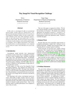


© Copyright 2026