
Annual Miles Drive Used Car Prices
Annual Miles Drive Used Car Prices
Maxim Engers
University of Virginia
Monica Hartmann
University of St. Thomas
Steven Stern
University of Virginia
January 2008
Abstract
Abstract: This paper investigates whether changes in vehicle’s net
bene…ts, proxied by annual miles driven, explain the observed pattern
of price declines over a vehicle’s life. We …rst model the household’s
decision on how much to drive each of its vehicles using two approaches.
The …rst is a basic nonstructural approach that restricts the relationship
between annual mileage and the household’s characteristics to be linear
over the vehicle’s life. The second is a structural model that allows for
nonlinearity. It takes into account how the composition of vehicles owned
- the number and the age distribution of the vehicles - in‡uence which
household car is drive on a particular trip and how much it is driven. We
then use the mileage estimates to determine if the variation in householdmileage decision across brands can explain the pricing paths observed for
used cars. Results indicate that the structural estimates of the household
mileage decision better predict changes in prices over a vehicle’s life. The
superiority of the structural estimates implies that the e¤ect vehicle age
has on mileage decisions (and consequently the vehicle’s market value)
cannot be estimated independently of household characteristics and the
composition of the vehicle stock owned. Thus, one must account for these
feedback e¤ects when using mileage to control for exogenously depreciated
quality. The results strongly suggest that variation in net bene…ts of
speci…c brand/vintage vehicles signi…cantly a¤ects variation in used car
prices.
Keywords: Annual Miles, Used Car Prices, Durable Goods
Corresponding Author: Steven Stern, Department of Economics, University of Virginia,
Charlottesville, Va 22904; [email protected]; (434)924-6754; fax: (434)982-2904.
1
1
Introduction
The net ‡ow of bene…ts provided by a vehicle can be viewed as the value of
transportation services provided minus the maintenance and repair costs incurred. Suppose that the annual mileage serves as a proxy for this ‡ow. Then
annual miles may explain the observed drop in used car prices over a vehicle’s
working life. This paper investigates what factors in‡uence household miles decisions and whether these choices are consistent with the observed pricing paths
of these assets.
There are a number of alternative explanations for why used car prices
decline with age, the pricing path we observe. One explanation is obsolescence
due to styling changes or quality improvements, such as airbags, advancements
that are available in newer cars.. For example, Purohit (1992) …nds that the
rate of depreciation on small vehicles increases with the introduction of a newer
model with greater horsepower. However, this obsolescence e¤ect, although signi…cant, is small relative to other durable goods that have more radical model
changes. Thus, it seems unlikely that improvements in car quality or in styling
changes can explain the magnitude of price declines and the variation in price
declines over brands. Another explanation is that the adverse selection problem
increases as vehicles age.1 For instance, Engers et al. (2005) provide evidence
that the used car market for four year old vehicles su¤ers more from adverse
selection than the one year old market. Still, it is questionable whether this is
su¢ ciently large to drive the decline in prices.
To determine if variation in vehicle usage (i.e., annual miles) helps explain
the observed price declines for automobiles, we …rst model the household vehicle
annual miles decision and then establish the empirical relationship between annual miles and used car prices. To estimate the household-vehicle annual miles
decision, we estimate two models: a basic OLS model and a structural model.
The OLS model assumes a linear relationship between household characteristics
and annual miles. In contrast, the structural model allows for nonlinear in‡uence of changes in car portfolios and household demographic characteristics on
how a vehicle’s age a¤ects annual miles. For instance, it takes into account
how the portfolio of vehicles owned - the number and the age distribution of the
vehicles - in‡uences a household’s decision to drive a car on a particular trip
and how much it is driven. Our results indicate that the structural estimates
of the household mileage decision better explain the observed pattern of price
decline over a vehicle’s life than the OLS model. Furthermore, the structural
model also allows us to decompose the age e¤ect of mileage on prices into three
parts: a direct aging e¤ect, a household-car portfolio e¤ect, and a household
demographics e¤ect. The …rst component captures the direct e¤ect vehicle age
1 One may argue that because of the vast improvements in car quality that adverse selection
is no longer a serious problem. According to J.D. Power & Associates’ Survey of Initial Car
Quality, the average number of car problems per 100 vehicles has declined signi…cantly in the
last 7 years. Despite these improvements, there is still variation across brands (e.g., Lexus
- 81, Mazda - 149, Suzuki -151). Furthermore, these …gures provide no indication about
the variability within a brand to make a statement that the adverse selection problem has
weakened.
2
has on annual miles. The portfolio e¤ect re‡ects the fact that annual miles
depend on the characteristics of the stock of vehicles the household owns. For
example, households often choose to drive the newer, more dependable vehicle
on long trips. Finally, the third e¤ect measures the in‡uence household characteristics, such as the number of drivers and whether or not the household lives
in an urban area, has on driving patterns. The superiority of the structural
model suggests that one cannot estimate the e¤ect age has on annual miles
decisions independent of household characteristics and household-car portfolio
choices. Thus, studies that measure the impact of adverse selection on prices,
for instance, miss these feedback e¤ects if they use only annual miles to control
for exogenously depreciated quality. They also must control for di¤erence in
driving patterns across households, vehicle age, and brand.
Our model of vehicle utilization and used car prices di¤ers from previous
studies. Goldberg (1998), using micro-level data, models annual miles as a
function of household demographic and vehicle characteristics as well as characteristics of the household’s stock of vehicles (e.g., number of vehicles, average
age of the stock, age of the youngest vehicle). Our study of vehicle utilization
di¤ers in three ways. First, we examine driving patterns over a vehicle’s entire working life and not just in its …rst year. Second, we investigate whether
driving patterns are constant across brands. Quality deterioration is known to
vary across brands. Thus, the value of the transportation services may vary by
brand and lead to di¤erent patterns of car usage over the vehicle’s working life.
Third, we examine if the amount a given vehicle is driven depends on its quality
relative to all of the other vehicles owned by the household and not just the
average quality of the household’s vehicle stock.
Our model of the process that generates used car prices di¤ers from Alberini
et al. (1995) (AHM1) and Alberini et al. (1998) (AHM2) as well. They estimate the distribution of vehicle values based on what owners would accept to
scrap their vehicles.2 Because their sample includes only vehicles that qualify
for a vehicle scrappage program, the average age is 17 years with a minimum
and maximum age of 13:5 and 32 years, respectively. Thus, they estimate the
distribution of vehicle values for only the right tail of the age distribution. In
addition to expanding the range of ages analyzed, our model allows annual miles
to play a di¤erent role in determining vehicle values. AHM1 and AHM2 model
household and vehicle characteristics directly determining the vehicle’s value.
Instead, we model these characteristics a¤ecting the vehicle’s value only indirectly through annual miles. Unlike AHM1 and AHM2, we …nd that household
characteristics are determinants of a vehicle’s value, but through their in‡uence
on annual miles. The intuition behind our result is that vehicle and household
characteristics a¤ects a household’s driving patterns and consequently a¤ects
the vehicle’s value as well.
Our …nding that vehicle age a¤ects annual miles nonlinearly also has implications for other automobile-related studies. For example, both Goldberg (1998)
2 The amount a household is willing to accept to scrap its car is weakly tied to the car’s
net bene…ts of transportation services. Alternatively, we use Kelly Blue Book used car prices
to proxy the car’s value that captures both supply and demand market conditions.
3
and Verboven (2002) assume annual miles are constant over the vehicle’s life.
Goldberg (1998) uses a model of vehicle utilization demand to estimate elasticity of annual miles demand with respect to gasoline cost per mile. Substitution
patterns derived from this model take into account di¤erences in fuel e¢ ciency
across new and used vehicles. Because it does not allow for di¤erences in vehicle usage across age, the model overestimates annual miles demand for older
vehicles and the reverse for newer ones, potentially biasing elasticity estimates.
Several data sources are used to establish the relationship between annual
miles and used car prices. Data from the National Personal Transportation
Survey allows us to track how much households drive each vehicle they own. The
survey also provides information on demographic characteristics that in‡uence
the amount of driving. Detailed pricing information is collected from Kelly Blue
Books. Finally, observed scrappage rates by brand are used to estimate jointly
the parameters of the process that determines used car prices and scrappage
rates, correcting for a potential selection bias problem in the price estimates.
The layout of the paper is as follows: Section 2 considers a simple dynamic
model of the relationship between annual miles and price to motivate the remainder of the paper. Section 3 describes the annual miles data and then
presents two alternative models to estimate household annual miles decisions.
Section 4 presents the model that jointly estimates prices and scrappage rates to
control for a selection bias. Section 5 examines the relationship between annual
miles and price and demonstrates that the structural model of household annual
miles decisions best explains the price decline observed in the used car market,
and Section 6 concludes.
2
Dynamic Model of Annual Miles and Price
The empirical results of this paper show that variation across brands in rates
of decline in annual miles explains variation in price declines across brands. In
order to understand these results, consider the following simple model of annual
miles and prices. Suppose that the bene…t ‡ow net of costs derived from owning
a car of brand b and age t is denoted by fbt which monotonically decreases with
t. We think of annual miles, the ‡ow of miles driven in one year, as a proxy
for fbt . Throughout the paper, we are interested in the ‡ow of miles driven
in one year rather than in the stock of miles previously driven. For simplicity,
suppose that the rate of decline in fbt is uniform over time (but can vary from
brand to brand), so that
fbt = & fb + fb t
(1)
where & fb > 0 and fb < 0.
If is the per-period discount factor, the value Wbt to any consumer of a
car of brand b of age t satis…es a simple recursion condition: the car can either
be sold at price pbt or kept for the period, generating current net surplus of fbt .
Thus
Wbt = maxffbt + Wbt+1 ; pbt g
(2)
4
Competition among buyers and the possibility of free disposal ensure that
pbt = maxfWbt ; 0g:
(3)
Because fb0 > 0 and fbt decreases at a constant rate, there is a (unique)
…nal period tb in which the vehicle provides a positive service ‡ow;
9tb : pbtb = Wbtb > 0; pbtb +k = Wbtb +k = 0 8k > 0:
Let Wbs denote the change in Wbs when s is increased by one, so that
Wbs+1 Wbs . In all periods t tb , Wbt = fbt + Wbt+1 , and so
Wbt =
By induction on tb
f
b
+
Wbt+1 8t < tb :
(4)
Wbs =
(5)
t, it follows that
Wbt < 0 8t < tb ;
(6)
so prices decline monotonically until the car becomes worthless. Di¤erentiating
gives
@ Wbt+1
@
f
b
=1+
@ Wbt+1
@
f
b
8t < tb ;
(7)
t,
and, again by induction on tb
@ Wbt+1
@
f
b
> 0 8t < tb :
(8)
This last relationship says that, if we compare two di¤erent brands, then
the one whose annual miles decline at a faster rate (i.e. whose fb is a larger
negative number) will also be the one whose price declines faster. The goal of
this paper is to see whether this relationship between the annual miles changes
and price changes is found in the data we examine.
3
Annual Miles
This section presents factors that in‡uence driving patterns. We …rst examine
relationships in the raw data between annual miles and household and vehicle characteristics. Then a simple OLS regression of log annual miles on these
characteristics provides insight into the in‡uence of each factor on driving patterns. Finally, we present a structural model that links annual miles choices with
household characteristics and the quality of the vehicles the household owns.
5
3.1
Data
The annual miles data for this study come from the Nationwide Personal Transportation Survey, 1995 (NPTS). The NPTS is a sample of 47293 vehicles owned
by 24814 households. We observe some characteristics of each household in
the sample such as family income, location characteristics (e.g., urban), and the
number of drivers disaggregated by age, gender, and work status. Also, we
observe each vehicle owned by the household, its age, brand, and annual miles
driven.
Table 1 reports moments of the data. The average household has a log
income of 5:93 ($37600)3 with 1:85 drivers and 1:91 vehicles. It has 0:2 teenage
drivers and 0:45 drivers who do not work, and it drives 23462 miles per year.
The average vehicle in the sample is 9:91 years old.
Figure 1 presents broad brand categories which will be disaggregated further
for most of the analysis. The categories included in the analysis are GM (Buick,
Chevrolet, Geo, Oldsmobile, Pontiac, Saturn); Japanese (Honda, Mazda, Mitsubishi, Nissan, Subaru, Toyota); Ford (Ford, Mercury); Luxury (American
Luxury,4 European Luxury,5 Japanese Luxury6 ); Chrysler (Chrysler, Dodge,
Plymouth); European (Volkswagen, Volvo); Truck;7 and Other.8 Trucks are
the most common category. Our method of aggregation is somewhat di¤erent than others in the literature. Goldberg (1998) aggregates into categories
of “subcompact,” “compact,” “intermediate,” “standard,” “luxury,” “sports,”
“pick-up truck,” and “van.” We feel our aggregation scheme is better for our
purposes because we think there are more likely to be brand e¤ects in the annual
miles decision. In fact, Goldberg’s results suggest that variability in car quality
based on car size is not a statistically signi…cant predictor of annual miles decisions.9 Thus, given that we are disaggregating by brand, not disaggregating
further by model causes a problem only to the extent that the mileage decision
is a¤ected by variation in car quality within a brand that is not correlated with
size. Berry et al. (1995) use a much …ner aggregation scheme. Using the
level of aggregation in their work would lead to inprecise estimates in our work,
especially given some of the sample sizes of complementary data used in related
work (Engers et al., 2004, Engers et al., 2005).
There are three measures of annual miles in the sample. We observe answers
3 Income
is measured in $100 units.
and Cadillac are aggregated throughout the analysis.
5 Audi, BMW, Jaguar, Mercedes-Benz, Porsche, and Saab are aggregated thoughout the
analysis.
6 In…niti and Lexus are aggregated throughout the analysis.
7 “Truck” includes all vehicles that are not automobiles.
8 The most common brands in “Other” are “not reported,” Hyundai, and Eagle.
9 Furthermore, there is no standard de…nition for vehicle size. Choo and Mokhtariam (2004)
reports alternative vehicle classi…cation schemes used in the academic literature and government agency reports. These studies primarily group vehicles either based on size, function
(e.g., sedan, coupe, truck), or both. In addition to no standard de…nition, the classi…cations
are not constant across time and thus somewhat arbitrary. For example, Consumer Reports’
“midsize”category has changed over time, particularly during the periods when the “compact”
category was eliminated (1980-1983 and 1995-present).
4 Lincoln
6
to questions of the form: “About how many miles was this vehicle driven?” The
time unit is a year if the vehicle was purchased more than a year ago, and it is
the tenure of the car otherwise. In either case, an annualized miles variable is
created. Also, we observe the odometer reading at the time of the interview
and a few weeks after the interview. Pickrell and Schimek (1999) report results
using reported annual miles and imputed annual miles based on the change
in the odometer (after adjusting for season, etc.) Their estimates look quite
similar to each other. Using the odometer reading, we also can construct a
measure of annual miles as a function of age by aggregating vehicles into cells
by age and brand and then di¤erencing the annual miles readings. Figure 2
shows how di¤erent estimates of annual miles vary with the age of the vehicle.
The estimate based on odometer reading is very imprecise and, in fact, for older
vehicles, is frequently negative. For the remainder of the analysis, we focus on
reported annual miles.10
Figure 2 shows a marked decline in annual miles as a function of age.11
This is consistent with previous work (Pickrell and Schimek, 1999). There are
many outliers in the annual miles data, so we checked to see if there are large
di¤erences between mean and median annual miles. While there are some differences, especially at late ages, these are not substantial enough to warrant
using orthogonal regression methods. One reason for the decline in annual
miles with age is that the vehicle becomes less useful and the household drives
the vehicle less. Lave (1994) suggests an alternative in which household heterogeneity causes some households to drive new cars many miles and then sell
them and other households to drive fewer miles and hold the cars longer. Rust
(1985) and Hendel and Lizzeri (1999) also have models of household heterogeneity with similar results. Later, in Section 5, we show that the household
e¤ects discussed in these papers are important in understanding the relationship
between changes in annual miles and changes in used car prices. In any case,
older vehicles are driven less than newer vehicles.
We can disaggregate the data by brand and then plot annual miles as a
function of age by brand. One can see signi…cant variation in annual miles
(negative) growth rates by brand. Figure 3 graphs the intercepts and slopes
of a log-linear regression lines for each brand. One sees signi…cant variation in
both base (annual miles of new cars) and annual miles growth rates. The three
brands with positive growth rates are Saturn (0:066), Japanese Luxury (0:049),
and Geo (0:033). All three of these cases have truncated age distributions
and are thus not that informative. However, even if these three are treated as
outliers, the remaining range in growth rates is still quite substantial, varying
from 0:094 (for Other) to 0:021 (for Volvo). It is also clear that growth rate
and base are negatively correlated.
1 0 We
…nd that the odometer reliability problem is not con…ned to the NPTS. Engers et al.
(2004) look at odometer readings and observe similar problems in the CEX. There, 8% of the
observations for which one is able to calculate quarterly miles using odometer readings give
negative results.
1 1 We can not control for variation in model year at the same time as age of the vehicle
because we have only a cross-section.
7
Household characteristics also might a¤ect annual miles. The most obvious
household characteristic is the number of drivers. Figure 4 shows the distribution of annual miles, disaggregated by the number of drivers in the household.
Among households with a single driver, 58% drive less than 15000 miles per
year, and 98% drive less than 40000 miles per year. Among households with
two drivers, only 28% drive less than 15000 miles, and 88% drive less than 40000
miles. There is a smaller increase in annual miles for households with three
drivers and then essentially no increase for households with more drivers. This
may suggest that a) there are economies of scale in driving12 or that b) not all
drivers are equal. Later we characterize drivers by their age, gender, and work
status.
Figure 5 is consistent with both (a) and (b) above. It shows that, while
vehicle ownership increases as household size increases from one to two, further
increases in household size have very little e¤ect on the number of vehicles in
the household. In all cases with household size greater than one, the modal
number of vehicles is two.
We also can observe how miles across vehicles within a household portfolio
vary with the number of vehicles in the household. Figure 6 provides such
information. In households with two vehicles, the best car13 is driven 65% of
the time (height of the …rst bar for rank 1), and the second best is driven 35% of
the time (height of the …rst bar for rank 2). In households with three vehicles,
the best is driven 52% of the time (height of the second bar for rank 1), the
second best is driven 33% of the time (height of the second bar for rank 2), and
the third best is driven 15% of the time. It is clear that, in households with
more than three vehicles, those beyond the third best have little e¤ect on the
usage of the …rst three best (each cluster ‡attens out after three vehicles). This
result is used later in the structural estimation of miles.
3.2
Nonstructural Estimates
In order to begin to understand what explains driving patterns, we …rst run
an OLS regression of log annual miles on vehicle and household characteristics
ignoring the nonlinear relationships suggested by Figure 4. The speci…cation
of the estimated model is
log mij
=
00
+
10 aij
+
K
X
0k bijk
+
k=1
+
K
X
2k bijk
iid 0;
2
h
;
min (aij ; 5) +
"ij
1k bijk aij
(9)
k=1
k=1
ei
K
X
iid 0;
H
X
3h Dih
+ ei + "ij ;
h=1
2
v
1 2 For example, 58% of single driver households drive less than 15000 miles, but 83% of
two-driver households drive less than 30000 miles, and 91% of three driver households drive
less than 45000 miles.
1 3 The best car is the one that is driven the most.
8
where mij is annual miles of vehicle j in household i, bijk is a dummy for
whether vehicle j is brand k, aij is the age of vehicle j, and Di is a vector of H
household characteristics.14 Though OLS is used to estimate ( 0 ; 1 ; 2 ; 3 ),
standard errors are corrected to account for household e¤ects captured by ei .15
The results are reported in Table 2.
The brand and brand/age interactions imply declining annual miles for all
brands over all ages with a few exceptions: Toyota, Mazda, Volvo, and European Luxury have modest annual miles increases for the …rst …ve years and
then signi…cant declines in subsequent years. Saturn has large increases and
then large decreases, but Saturn estimates are very imprecise. In all cases,
declines in log annual miles are steeper after age 5 than before age 5.
Wald tests for H0 : 0 = 0 and H0 : 1 = 2 = 0 against the general
alternatives are statistically signi…cant at the 1% level of signi…cance. The
results also suggest that household income increases annual miles, and living in
an urban area decreases annual miles. The latter result would follow from the
closer proximity of places of interest and the higher cost of driving in tra¢ c.
While there are o¤setting e¤ects such as the greater abundance of places to go
and higher costs of living close to work, the former e¤ects dominate empirically.
The addition of other vehicles in the household decreases annual miles on each
vehicle as Figure 6 suggests. Annual miles generally increases with drivers,
especially working and adult drivers. Males drive more than females. A Wald
test for H0 : 3 = 0 against HA : 3 6= 0 is statistically signi…cant at the 1%
level of signi…cance.
3.3
Structural Estimation Method
The OLS regression reveals basic factors that in‡uence driving patterns across
households and their vehicles. This section presents a structural model that formally incorporates the nonlinear relationship between annual miles and number
of drivers as evident in the data. We model annual miles choices as being determined by a two-stage process that …rst determines the number of trips and
then determines the choice of car for each trip. The demand for trips is a function of the household’s demographic characteristics and the quality of vehicles
it owns. The choice of car to use for each trip is a random utility choice where
the value of each mode for the particular trip has a deterministic component
plus an iid Extreme Value error. This structure is the same structure as in
models of brand choice such as Berry et al. (1995). There, one models the
choice of each decision maker and then aggregates over decisionmakers to …nd
shares. Here, one models the vehicle choice for each trip and then aggregates
over trips to …nd annual miles shares for each household vehicle.16
1 4 The
inclusion of the min (aij ; 5) term allows for a spline in age with a node at 5 years.
variance parameters, 2h and 2v , are estimated by matching second sample moments
to theoretical moments implied by 2h and 2v .
1 6 Technically, we also must assume that all trips are for one mile. However, since we have
no data on trip distances, it is both unlikely we could identify the parameters of a richer
speci…cation and unlikely that the violation of our assumption a¤ects results in a signi…cant
1 5 The
9
Let mij be annual miles of car j in household i, j = 1; ::; Ji , and
mi =
Ji
X
mij :
(10)
j=1
Let household i have demographic characteristics Di and car j of household i
have characteristics Cij . We can model
mij
mi
= g (j; Ci ; ui ; ) mi ;
= h (Ci ; Di ; ui ; )
(11)
where Ci = (Ci1 ; Ci2 ; ::; CiJi ), ui = (ui1 ; ui2 ; ::; uiJi ) is a vector of errors, ui
iidN 0; 2u I , and is a vector of parameters speci…ed below. The data suggest
that, even for households with 4 or more cars, the characteristics of only the 3
best cars matter in the h function (see Figure 6).17
Let the value of car j be18
Vij = Cij + uij ;
(12)
and let Ri (j) be the rank of car j in household i according to Vij ; i.e., Ri (j) <
Ri (k) i¤ Vij > Vik and Ri (j) 2 f1; 2; ::; Ji g.19 Let S ( ) be the inverse of Ri ( ).
We model h semiparametrically using polynomials with imposed monotonicity. In particular, de…ne p0 (v) 1 and
pj (v) =
M
X
jm v
m
(13)
m=1
as an M th-degree polynomial in v for j > 0. Let
8
if j = 0
< 0
ViS(j)
if j = 1
ViS(j) =
:
ViS(j) ViS(j 1) if j > 1
;
(14)
i.e., ViS(1) is the value of i’s best choice, and ViS(j) is the negative of the
marginal reduction in value between the jth best choice and the (j 1)th best
choice for j > 1. De…ne Ji = min (Ji ; 3) and
[Ji ; Vi ] =
Ji Ji
X
X
jk pj
ViS(j) pk
ViS(k)
(15)
j=0 k=j
way.
1 7 Figure 4 shows that the marginal e¤ect of drivers after the second driver is small also.
However, we use characteristics of all of the drivers because it is easy to do so and it is not
obvious how to rank drivers.
1 8 One should note that we do not allow the value of car j to depend upon the household’s
demographics. Berry et al. (1995) found valuation of vehicle characteristics (e.g. miles per
gallon, size) varied across income groups, and one might expect these vehicle characteristics
to in‡uence how much a vehicle of a particular brand is driven. For instance, Hondas with
high mpg may be driven over longer distances than Volvos with low mpg. While these are
good arguments, since we use only age and brand as car characteristics, we think it unlikely
we could measure household demographic/car characteristic interactions with any precision.
1 9 We ignore ties because they occur with zero probability.
10
as a product of polynomials in di¤erent combinations of ViS(j) and ViS(k)
with 00 = 0 and 01 = 1. We think of [Ji ; Vi ] as a semiparametric approx3
imation of a general function in
ViS(j) j=0 in the sense that, as the sample
size increases, we can increase M (and also the number of ranked cars in the
function from 3). This point is formalized in the Appendix.
Ji
Note that [Ji ; Vi ] is equivalent to a function in ViS(j) j=0
that can be
constructed by expanding equation (15) and then collecting terms appropriately.
The speci…cation in equation (15) is preferred because it makes it easier to
impose conditions such as @ [Ji ; Vi ] =@ ViS(j) declining in j.20 Consider the
special case where jk = 0 for all j > 0 and only linear terms (= 1) occur in
equation (13); i.e.,
Ji
X
[Ji ; Vi ] =
(16)
0k ViS(k) :
k=j
Then, for example, if all car values increase by 1, [Ji ; Vi ] increases by 1; and,
if just the best car increases in value by one, then [Ji ; Vi ] increases by 1
02 .
All of the remaining jm terms in equation (13) and jk terms in equation
(15) allow for nonlinearity. The jm terms allow ViS(k) to enter [Ji ; Vi ]
nonlinearly, and the jk terms allow for interactions among the pj
ViS(j)
terms.21
We could model h (Ci ; Di ; ui ; ) as a function of [Ji ; Vi ] and Di , but such a
speci…cation would allow for the possibility that [Ji ; Vi ] would have some estimated negative partial derivatives. Stern (1996) found that, without imposing
monotonicity on a semiparametric function of two arguments that theory implied should be monotone, the estimated function deviated far from a monotone
function. Mukarjee and Stern (1994) and Stern (1996) suggest a simple method
to impose monotonicity, similar in spirit to Matzkin (1991), and we use an analogous method here. For any function f : W ! R where W is a nonempty subset
of RJ for some J, de…ne
[f ] (x) = sup [f (y)] :
(17)
y x
transforms the function f into a new function
all of its arguments. In fact,
[f ] g
[f ] that is nondecreasing in
(18)
for all nondecreasing g such that f g. We use the [ ] transformation because
annual miles by household should be increasing in the vector of V values. We
model
log h (Ci ; Di ; ui ; ) = [ ] + Di
(19)
2 0 We
specify equation (19) in terms of ViS(j) rather than ViS(j) also because the optimization method performs signi…cantly better. This speci…cation implies that ViS(j)
0
for all j > 1.
2 1 Some terms are not identi…ed separately; e.g. the linear term in
and the linear term in
.
11
as a partial linear equation, ‡exible in car values and linear in household characteristics. We approximate the function by discretizing the V -space and then
checking for monotonicity in h point by point. This sounds computationally
intensive, but, in fact, its cost is proportional to the number of grid points.
We assume that the g function depends on Ci and ui only through the e¤ect
of Ci and ui on Vi = (Vi1 ; Vi2 ; ::; ViJi ), and it depends on j only through Vij and
Rij = Ri (j). Let
exp f (Vij ; Rij ; )g
j 0 exp f (Vij 0 ; Rij 0 ; )g
where
(Vij ; Rij ; ) =
g (j; Ci ; ui ; ) = P
( P
Ji
1
k=Rij
! k ViS(k)
ViS(k+1)
0
if Rij Ji
if Rij = Ji
(20)
1
(21)
is a spline function (in slopes) in Vij with nodes at the values of the ranked Vi ’s.
This is a weighted logit function that allows for ‡exibility with respect to how
ranking interacts with car value. Note that it is increasing in each element of
Vi (assuming ! k is positive 8k) and that, if ! k = 1 8k, then g (j; Ci ; ui ; ) is
a logit function. While there is no explicit “outside option” in equation (20),
we allow for an outside option by modelling the total demand for annual miles
in equation (19). Finally, the functional forms of equations (19) through (21)
satisfy the conditions described in Berry et al. (1995) for a unique solution in
ui to the set of equations,
mij
= g (j; Ci ; ui ; ) ; j = 1; 2; ::; Ji ;
mi
(22)
log mi = log h (Ci ; Di ; ui ; ) :
(23)
De…ne u
bi as the value of ui that satis…es equations (22) and (23). If we decompose u
bi into u
bi1 and u
bi=1 = (b
ui2 ; u
bi3 ; ::; u
biJi ), then, conditional on any value of
ui1 = u0i1 , there is a unique solution u0i=1 to equation (22). Furthermore,
@u0ij
= 1 for all j
@u0i1
(24)
because of the usual location identi…cation problem in random utility models.
The value of u
bi1 is the value that solves equation (23).
We ignore endogeneity problems. In particular, households that require a
lot of annual miles (large ui ) will purchase vehicles of greater quality (larger
Vij ). More importantly, households that like to drive (large ui ) may also like
to have higher quality vehicles (larger Vij ) independent of their need for annual
miles.22
Thus, the estimates of in equation (13) may be biased upwards.
2 2 Verboven (2002) models the choice of car make, focusing on whether to buy a car with
a gas or diesel engine, given desired annual miles of the household. While we ignore the
endogeneity of brand choice, he ignores the endogeneity of annual miles.
12
Given the nature of the data, all we can do here is acknowledge the problem
and interpret results with caution.23
The set of parameters to estimate is =
; ; ; ; !; 2u where is the
e¤ect of car characteristics Cij on car values Vij in equation (12), is the e¤ect
of demographic characteristics Di on total household annual miles in equation
(19), is the set of polynomial coe¢ cients in equation (13),
is the set of
weights on each of the polynomial products used to determine the total value of
the household’s car portfolio in equation (15), ! is the set of weights determining
how car shares depend upon relative values in equations (20) and (21), and 2u is
the variance of the unobserved household heterogeneity in equation (12). The
log likelihood contribution of family i is
Li =
Ji
X
j=1
log
1
u
u
bij (Ci ; )
u
log j ( )j
(25)
where [ ] is the standard normal density function and ( ) is the Jacobian.
Our model speci…cation di¤ers signi…cantly from other models of demand
for annual miles. For example, Goldberg (1998) uses a model similar to Dubin and McFadden (1984) to measure the joint decision of buying a new car
and how many miles to drive it. The technology available in Dubin and McFadden (1984) controls for the selection bias in annual miles associated with
brand choice. As stated above, we ignore this selection bias. On the other
hand, while we have a rich speci…cation of how annual miles decisions for each
car in a household’s portfolio interact, Goldberg includes only aggregate characteristics of the household’s portfolio (average stock age, age of newest car,
whether any other cars are owned, and number of cars) and estimates a miles
equation for only the new car recently purchased.24 Mannering and Winston
(1985) construct a dynamic model of car choice and utilization but also do not
really allow for any interaction across cars within a household in simultaneous
decisions about how much to use each car.25
3.4
Results for Structural Speci…cation
We estimate a number of di¤erent speci…cations of the structural model of the
household’s decision of how much to drive each vehicle it owns. The speci…2 3 We cannot use the methodology developed in Verboven (2002) because our problem is
more complicated. In particular, Verboven (2002) assumes each household owns only one
car. While this assumption re‡ects European household vehicle stock in the early 1990s,
the sample period for this study, a quarter of western European households now own two
or more vehicles (Ingham, 2002). This assumption is further violated in the U.S. where
the average household owns 1.91 vehicles. Because we are using U.S. data and Verboven’s
methodology relies heavily on the one vehicle per household assumption, we had to develop
another methodology to examine household annual miles decisions.
2 4 Our model suggests that Goldberg’s aggregated portfolio characteristics could never be a
su¢ cient statistic for all of the characteristics of the portfolio. For example, while the number
of cars matters, it must be interacted with some measure of the quality of each of the cars.
2 5 In their model, the use of a car today a¤ects the use of similar cars in the future because
it a¤ects perceptions of the car. However, there is no decision today about how to allocate
driving miles among cars in the household portfolio.
13
cation we focus on, reported in Table 3, restricts in equation (13) to linear
functions26 and the higher order shape parameters ( in equation (19))27 and
reports estimates for ! in equation (21), car characteristic e¤ects ( in equation
(12)), demographic e¤ects ( in equation (19)), and log u in equation (12).28
This allows for the value of each vehicle to in‡uence log household annual miles
‡exibly. We allow (in ) for brand e¤ects and brand-age interaction e¤ects
as we did in the nonstructural model. Most of the estimates are statistically
signi…cant, and almost all of the brand-age e¤ects are negative after adding the
age slope e¤ects.
Many of the estimates in Table 3 are di¢ cult to interpret. Starting with the
! shape parameters in equation (21), recall that the number of annual miles
driven on a given vehicle depends on its value relative to the other vehicles
owned. Thus, ! k captures how the relative value of the kth car to the next best
vehicle a¤ects the multinomial logit share of household miles driven on that
vehicle. Consider a family with three vehicles. The log ratio of the model’s
choice probability for the choice with the best V to a multinomial logit model’s
choice probability for the choice with the best V is displayed in Figure 7 for
di¤erent values of Vi2 and Vi3 . The log ratios are always positive because
!
b 2 > ! 1 = 1; this implies that values for third choices (or lower) receive less
weight than values for the second choice. In particular, we can write the
probability of the …rst choice as
P1 =
exp f! 1 V1 + (! 2 ! 1 ) V2 g
exp f! 1 V1 + (! 2 ! 1 ) V2 g + exp f! 2 V2 g + exp f! 2 V3 g
(26)
which converges to a multinomial logit probability as ! 2 ! ! 1 and is greater
than the multinomial logit probability when ! 2 > ! 1 . Also note that the choice
probabilities given our speci…cation still have the independence of irrelevant
alternatives property (after conditioning on u), so Figure 7 displays also the log
ratio probabilities for the second best choice.
The coe¢ cients in equation (15) capture how the (total) household annual
miles is dependent on the nonlinear relationships between the relative values
of di¤erent combinations of vehicles from which the household takes on trips.
Since we estimated only linear terms, the h ( ) is linear as well.
The results we are most interested in are the age e¤ects. When interpreting
the age e¤ects on the annual miles decision, consider that, for the most valuable
26
= 1 and j2 = 0 for j = 1; 2; 3:
= 1 and 01 = 1 (for identi…cation), jk = 0 8j 6= 0; 1 = 1, k = 0 8k 6= 1.
2 8 We estimate a third speci…cation adding the nonlinear
terms and …nd that it behaves
very poorly. It is clear that adding such terms leads to severe over…tting of the data as is
common in using polynomials to approximate functional form.
27
j1
00
14
car in a household portfolio,29
@ log mij
=
@Ageij
[1
g (j; Ci ; ui ; )] +
1
h (Ci ; Di ; ui ; )
(
Age
+
Brand-Age ) ;
(27)
while, for the second most valuable car,
@ log mij
=
@Ageij
[1
g (j; Ci ; ui ; )] (! 2
1) +
02
h (Ci ; Di ; ui ; )
(
Age
+
Brand-Age )
(28)
(note that !
b 2 1 = 0:456 and b02 = 1:931). However, since Age does not vary
over brands (b Age = 0:302 if Age
5 and b Age = 0:337 if Age > 5), one
can compare variation in age e¤ects over brands by focusing just on the BrandAge estimates. One should note that the thought experiment corresponding
@ log m
to @Age ij is not to let the car age one year; rather it is to sell the car and
ij
purchase a car of the same brand one year older. The importance of this point
becomes clear in Section 5.
Probably, a more fruitful way to understand age derivatives in the structural
speci…cation is to directly evaluate and graph average derivatives of log annual
miles with respect to age. Such derivatives vary by brand, age, household-car
portfolios, and household characteristics. In Figure 8, we aggregate over households, therefore averaging over household-car portfolio and household characteristics e¤ects. Figure 8 shows how average derivatives for a selected subset of
brands vary with brand and age. The average derivatives are mostly negative
and declining with age. Of those not represented in Figure 8, only Dodge has
positive age derivatives; the other 16 are all negative and declining with age.
We also can measure how the usage of other cars in the family changes as a
particular car ages. The implication of the vehicle annual miles share function
in equation (20) is that, as a particular car ages (holding all else constant), it
becomes less valuable (because the relevant estimated total e¤ects are generally negative), thus increasing the shares of the other cars in the household’s
portfolio. On the other hand, the household total miles function in equation
(19) implies that total household miles decline. The structural estimates imply
that the net e¤ect is very small and negative, averaging about 0:4% per year.
We also can measure how demographic characteristics a¤ect car usage. The
estimates in Table 3 measure
in equation (19), the e¤ect of demographic
characteristics on total miles. We do not interact demographic characteristics
with car characteristics. Thus, the demographic derivatives do not vary over
cars or over age. The results also suggest that vehicle utilization varies across
households with varying numbers of drivers. Annual miles rises with the number
of adult drivers, male drivers, and working drivers in the household, but falls
2 9 Note
that, for multinomial logit probabilities,
@ log P
P (1 P ) @P
=
= (1
@A
P
@A
15
P)
@P
:
@A
with other types of drivers. Finally, household income increases annual miles,
but unlike with the OLS estimates, living in an urban area raises annual miles.
4
Prices
In the previous section, we show that annual miles falls as a vehicle ages. Before
we can ascertain the relationship between annual miles and prices, we explore
the extent to which scrappage rates explain price declines. We jointly estimate
used car prices and scrappage rates as a vehicle ages. Then we examine if we
need to correct for a selection bias; poorer quality vehicles are scrapped …rst
biasing the estimates of price declines.
4.1
Data
The price data for this study come from the Kelley Blue Books over the period
1986 - 2000.30 The price data are generated from sales reports to the National
Automobile Dealer’s Association (NADA) provided by member dealers. For
each year in the sample period, we observe the average price of each brand of
car for each relevant manufacturing year.31 For example, in 1990, we observe
the average price of multiple models for each brand for the 15 model years
from 1986 - 1990 inclusive. We observe 8887 prices and 7918 changes in price.
The mean price is $10797, and the standard deviation is $8463. The price
range is from $825 to $97875. The average change in log prices is 0:133, and
its standard deviation is 0:077. One can see in Figure 9 that there is a large
percentage price decline in the …rst year and then smaller declines in subsequent
years. When vehicles reach 12 years of age, price declines signi…cantly diminish.
We argue below that this can be explained by a scrapping e¤ect. Table 4 shows
how price changes vary by brand.32 There is signi…cant variation by brand
with Honda and Toyota having the smallest average price declines and Isuzu
and Hyundai having the largest average price declines. American cars tend to
have larger than average price declines.
Finally, the scrapping data used in this study are from R.L. Polk & Co. The
scrapping rates are observed reductions in the stock of cars of each brand as a
proportion of the stock the year before. We observe scrapping rates only for
3 0 See Porter and Sattler (1999) for a more detailed discussion of the quality of the Blue Book
data. Alternatively, one could use transaction prices to capture car-speci…c quality. However,
these transaction prices also re‡ect the relative bargaining power of the buyer and seller and
other characteristics idiosyncratic to the particular car. If we were to uses transactions prices,
we would average them just as Kelly Blue Book did to average out any car-speci…c e¤ects.
3 1 Prices based on the base model, four-door sedan model are used whenever possible. When
matching the price data with the vehicle data in the NPTS, we assume all cars are sold at
the base model price. Thus, we lose some variation in prices within a brand-model, but do
capture the variation in prices across brand-models.
3 2 The truck category was dropped because we lack price data. NADA records price information for trucks in a separate publication from the one that reports passenger vehicle prices
used for this study. The other category was also dropped and the Isuzu and Hyundai brands
were added in place because we had detailed price information on cars in this category.
16
eight car categories and only for a limited number of relevant vintages.33 So we
use nearby substitutes for other brands and use scrapping rates for cars manufactured in 1990. Also, we ignore the …rst two years of the car because observed
scrapping rates are actually negative as car dealers sell their remaining stock.
The substitution pattern is reported in Table 5. One might worry that scrapping rates are not constant over time and thus it is problematic to use scrapping
rates for cars manufactured in just 1990 to proxy for all scrapping rates. However, we have no data on scrapping rates disaggregated over both calendar time
and brands. Also data from Ward’s Communications (2001), shown in Figure
10, show that, once after initial volatility in scrapping rates (across calendar
time), scrapping rates are relatively stable. Most of the selection e¤ect occurs
at these later ages.
4.2
Pricing Estimation Method
Given the data described above, we can estimate a pricing function for passenger
vehicles controlling for scrappage. Assume the price of car j of brand i at age t
is
pijt = it + ij
(29)
2
(30)
i t:
(31)
iidN 0;
ij
with
it
=
i
+
Let pit be the average observed price of brand i cars at age t, and let dit be the
scrapping rate of brand i cars at age t. Scrapping occurs because some fraction
d are totaled or otherwise exogenously disappear and because some cars have
nonpositive value. We observe only positive prices; cars with negative prices
are junked. The joint moments of (pit ; dit ) are
o
n
R1
2
p1
it
(
+
)
exp
it
2 2 d
2
it
o
n
;
(32)
=
+
Epit =
R
it
2
it
1
p1
d
exp
2
2
2
it
n
o
R it
2
1
p
it 1
it
d
exp
2
2
2
it 1
n
o
Edit = d +
=
d
+
:
R
it
1
2
1
p1
exp
d
2
2
2
it
1
n
n
In the data, we observe fpi1 ; pi2 ; ::; piT gi=1 and fdi1 ; di2 ; ::; diT gi=1 for some
0
subset of n car brands. Let yit = (pit ; dit ) , let = ( ; ; ; d ) be the set of
parameters, and consider minimizing the objective function,
L( ) =
3 3 The
1 X
(yit
nT i;t
0
Eyit )
(yit
Eyit ) :
Polk scrapping rate data were given to us by Matthew Shum.
17
(33)
The asymptotic distribution of the estimates is
p
nT b
N (0; )
(34)
with
= B
1
2
plim 4
E (yit
b
1 X @E yit j
nT i;t
@ 0
E (yit j )) (yit
where
B = plim
4.3
(35)
0
E (yit j )) j
1 X @E (yit j
nT i;t
@ 0
0
@E yit j b
) @E (yit j )
:
@
@
3
5B
1
(36)
Pricing and Scrappage Results
The pricing and scrappage parameter estimates are reported in Table 6.34 All
of the estimates are highly signi…cant. The most important parameters are the
estimates of and d . The estimate of log is 1:345 implying an estimate of
of 3:838. While we think this may be a bit high, it is necessary to explain
the curvature in the price curve and the increase in scrapping rates as cars age.
The estimate of d is 0:0091. The estimate of d is very close to the observed
scrapping rates of four year old cars. This is what should be expected.
One can perform a residual analysis to see how well the model …ts the data.
De…ne
edit
= dit
epit
= pit
E dit j b ;
(37)
E pit j b :
Table 7 reports average residuals for scrapping rates and prices aggregated by
brand, and Table 8 reports the same aggregated by age. Though most of
the average residuals are statistically signi…cant, most are small in magnitude.
Note that, for brand-speci…c residuals, almost all of the brands have average
scrapping rate residuals and price residuals of the same sign. In cases where
this is not so, then the pricing parameters ( i ; i ) can adjust to reduce the absolute value of both residuals. The residual analysis suggests that Nissan,Volvo,
3 4 Additional brands were dropped because we do not have scrappage rates on their close
substitutes to estimate the joint moments of (pit ; dit ). Those dropped were the three luxury
brands, Geo, Hyundai, Saturn. Alternatively, one could estimate a hazard function for vehicle
scrappage. Chen and Niemeier (2005) estimate retention rates by vehicle class (all passenger
vehicles were in the same class). They use smog check data collected by the California Bureau
of Automotive Repair. But because vehicles under age 5 are exempt from inspection, a full
hazard function cannot be estimated for our purposes.
18
Honda, and Dodge are bad …ts.35 Part of what may be occurring, especially for
Nissan, Honda, and Volvo, is that manufacturers signi…cantly change their cars
across model years during the sample period leading to di¤erent prices paths
across model years (or sets of model years). For example, the 3rd generation
Honda Accord arrived in 1986, and Accords were upgraded when the 4th generation Accord arrived in 1990. Thus, there may be di¤erent price paths for
pre and post 1990 Honda Accords. Because of this, a composition e¤ect may
be contaminating our results for these brands. It also suggests that our model
is not rich enough to explain the nonlinearity in observed average pricing and
its interaction with scrapping rates. In particular, we overestimate scrapping
rates at ages t
12. This is partly true because used car prices depend on
many factors not controlled for in this study such as the vehicle’s equipment
and condition. While these factors in‡uence actual transaction prices, they do
not a¤ect the Kelly Blue Book value. This value is just a starting point for
dealers to estimate a vehicles’worth and does not take into account car-speci…c
factors. Thus, controlling for additional factors would not improve the model’s
predictive power of Kelly used car prices across vehicle age.
Lastly, we examine if one must correct our results for a selection bias. Used
car prices represent the average price of automobiles still in use in time t and
not the average price of vehicles in the original cohort. Failing to control for the
scrapping of poorer quality vehicles …rst would bias upwards the rate of decline
in prices. In order to compare how alternative speci…cations …t the data, we can
plot the observed price path, the predicted price path ignoring selection, and
the predicted price path taking into account selection. For example, the price
paths for Oldsmobiles are shown in Figure 11.36 For most brands, our model
is very precise in predicting the price paths after controlling for the selection
bias. However, there is something about the price paths for Honda, Volvo, and
Volkswagen that we miss. In particular, we cannot explain increasing price
paths with our selection model when the underlying randomness is normal.
We also can plot scrapping paths.37 We can not explain nonmonotone scrapping rates and, in general, we miss the scrapping rates by signi…cant amounts.
This occurs basically because the terms in in equation (33) associated with
edit and epit in equation (37) gives more weight to epit than edit .
3 5 This also may be due to not controlling for how the market perceives changes in vehicle
models. Purohit (1992) shows that if the market perceives a new model is less preferable than
earlier models, then the demand for used versions of these vehicle rises, increasing their used
prices (and vice versa). These shifts in the price paths would not be captured by our model.
3 6 Price paths for each brand are available at
http://faculty.virginia.edu/stevenstern/resint/empiostf/selection_gi¢ les/paths.html.
3 7 Scrapping
paths for each brand are available also at
http://faculty.virginia.edu/stevenstern/resint/empiostf/selection_gi¢ les/paths.html.
19
5
Relationship Between Annual Miles and Price
Now that we have estimated the process that generates both annual miles and
pricing, we can investigate the relationship between these two processes. The
estimates of from equation (9) in Table 2 tell us how log annual miles declines
with age, disaggregated by brand, and the estimates of from equation (31) in
Table 6 tell us how log prices decline with age, disaggregated by brand.38 We
can compare annual miles and price decline estimates to see if the two processes
are moving together. This is done in Figure 12. The OLS estimates of the
linear relationship between them are
bj =
0:791 + 6:75bj + uj :
(38)
The t-statistic on the bj coe¢ cient is 2:00, and the R2 is 0:21. This, along with
the price/maintenance results in Engers et al. (2004), suggests that declines in
annual miles might explain declines in price as a car ages.
Consider using the structural average derivatives with respect to age, some of
which are shown in Figure 8, to explain the change in log prices. The estimated
slope is 0:557, and R2 = 0:020. So the obvious question is why the OLS estimates explain prices pretty well and the structural estimates do not. The answer
is that the two sets of estimates are measuring very di¤erent objects. In particM iles
jDem ographics,Portfolios ; i.e.,
ular, the structural estimates are measuring @ log
@Age
unlike the OLS estimates, they are holding constant demographic e¤ects and
household-car portfolio e¤ects. We can interpret these di¤erences in light of the
model of car turnover in Rust (1985) or the base model in Hendel and Lizzeri
(1999) (with no transactions costs or asymmetric information problems). In
these models, because there are no transactions costs or asymmetric information
problems, each household sells its cars every period. Changes in prices as the
M iles
car ages re‡ect both @ log
jDem ographics,Portfolios and the changes due to the
@Age
movement of cars to di¤erent household types as the car ages.
We would like to measure the demographic e¤ects and household-car portfolio e¤ects but do not have enough data to estimate models of portfolio choice.39
However, we can construct semiparametric estimates of total average derivatives
(allowing demographic characteristics and household-car portfolios to change).
Using our structural estimates, we construct an estimate of the total derivative
for each car j in household i in our sample. Let bij be the brand of car j in
household i and aij be its age. De…ne ij = Di b (from equation (19)) as a
propensity score for household demographic characteristics in the spirit of Rubin (1979), Rosenbaum and Rubin (1983), and Heckman et al. (1998) and as
3 8 Since
we aggregate car makes in the NPTS and Kelley Blue Book data the same way,
we have no problem matching annual miles slope estimates from Table 2 with price slope
estimates from Table 6.
3 9 The fact that the NPTS is not a panel prevents us from measuring changes in portfolios.
20
a bandwidth.40 Then our estimate of the total derivative is
P
i0
i0 j 0 1 (bi0 j 0 = bij ) 1 (ai0 j 0 = aij + 1) K
@ logd
Milesij
=
P
@Age
+ 1) K
0 0 1 (b 0 0 = b ) 1 (a 0 0 = a
ij
ij
ij
ij
ij
i
i0
log mi0 j 0
i
log mij
(39)
where 1 ( ) is the indicator function and K ( ) is a kernel function. Note that we
condition on cars having the same brand and being one year older. We use two
separate kernel functions. First, we set K ( ) 1. This choice of kernel function
causes averaging over varying demographic characteristics of households owning
cars of brand bij with age equal to aij +1. Then we set K ( ) equal to a standard
normal density function truncated at 4. This choice of kernel function controls
for household demographics; i.e., we weight more heavily the annual miles of
cars i0 j 0 in households with similar demographic characteristics Di0 to household
i’s characteristics Di (where similarity is measured in terms of the propensity
scores).
Using the estimates from equation (39), we construct median derivatives
disaggregated by brand and disaggregated by brand and age. We use median derivatives because mean derivatives are unduly in‡uenced by outliers. In
fact, Figure 13 shows how median derivatives, disaggregated by age, vary over
age. The three di¤erent derivatives shown are: 1) “Age” plots the derivative
holding demographic characteristics and portfolio choices constant, 2) “Total”
plots the derivative holding only demographic characteristics constant, while
3) “No Demographics” plots the derivative when both demographic characteristics and vehicle portfolio are allowed to change. Note that, while the “Age”
curve behaves well, the other two curves are poorly behaved. Curves for other
brands look similar. Figure 14 presents the distribution function of derivatives
(censored at 0:5) for Chrysler aggregated over age (other brands have similar
graphs). While there is some mass in between the censoring points (in fact
the median is always strictly between the censoring points), most of the mass
is beyond the censoring points.
The plim of an OLS estimate in the presence of measurement error in the
2
2
2
is the true value of the linear
explanatory variable is
x=
x + e where
2
slope term, x is the sample variance of the explanatory variable, and 2e is the
variance of the measurement error.41 Under the assumption that a sample of
random
variables is iid, the standard deviation of the estimate of a median is
p
1
[2 nf ( )] where n is the number of observations used to estimate the median
and f ( ) is the density of the random variables evaluated at the median (e.g.,
Bickel and Doksum, 1977, p. 400). The estimated standard deviations of the
median estimates and corresponding bias ratios ( 2x = 2x + 2e ) are listed in
M iles
Table 9. The estimated median partial derivative @ log
jDem ographics,Portfolios
@Age
is measured very precisely relative to the variation across brands x . But the
estimates of the total derivatives have large standard deviations.
4 0 We
use one quarter of the standard deviation of the propensity score as the bandwidth.
the more general case where there is heteroskedasticity in
Pthe2 measurement error across
observations (as is true here), the term 2e is replaced by n 1
ei .
4 1 In
21
Figures 13 and 14 and Table 9 suggest that the derivatives estimated using
equation (39) are problematic. However, we proceed to use them in a regression similar to equation (38). We do this partially because there is no better
alternative and partially because, even though the biases of the OLS estimates
are large, the R2 statistics (and therefore t-statistics and F -statistics) have no
asymptotic bias.42 The results are presented in Table 10. The …rst row of Table
10 repeats the results of equation (38), and the second row repeats the results
using the partial derivatives already discussed. The last two rows correspond to
using K ( ) equal the truncated normal density and K ( ) 1 respectively. The
M iles
jDem ographics,Portfolios have no explanatory power for
partial derivatives @ log
@Age
price changes. For the linear semiparametric speci…cation, the partial derivative
is negative, casting more doubt on the credibility of the linear semiparametric
M iles
estimates. On the other hand, the total derivative @ log
and the derivative
@Age
M iles
jDem ographics both explain price changes
controlling for demographics @ log
@Age
as well as the OLS equation from Figure 12.43 When we further consider that
the implication of Figure 14 is that median derivatives are measured with signi…cant error (and we know that measurement error in an explanatory variable
causes bias towards zero), we conclude that the structural estimates explain
the price changes better than the OLS equation. These results suggest that
portfolio e¤ects and turnover e¤ects in the spirit of Rust (1985) and Hendel and
Lizzeri (1990) are important in explaining price changes as cars age.
The results also demonstrate the value of the structural estimates. While
the OLS estimates in equation (38) provide a useful measure of the total e¤ect
of aging on car prices, they can not be used to decompose the aging e¤ect into
its components: the direct aging e¤ect, the household-car portfolio e¤ect, and
the household demographics (or car turnover) e¤ects. The structural estimates,
along with information about the distribution of cars across households, allow
us to decompose the e¤ects.
4 2 This
result is not as well known as the bias result. However, given the linear model,
y =x +u
with
R2 =
w
=
x + e;
y
=
wb + v;
0
(wb) (wb) =n
b0 (x + e)0 (x + e) b=n
=
0
y y=n
(x + u)0 (x + u) =n
and
plimR2 =
2 2
x
2
x
2
e
2 + 2
x
e
2 2
2
x+ u
=
2 2
x
2 2
x
+
+ 2u
which is independent of measurement error in x.
4 3 Note that multiplying the reported estimates for the total derivative and the derivative
controlling for demographics by the inverse of the associated bias terms in Table 9 results in
an estimate very similar to the OLS derivatives.
22
6
Conclusion
The objective of this paper is to determine if changes in a vehicle’s net bene…ts,
proxied by annual miles, explain the observed decline in used car prices over
the vehicle’s life. We …rst model the household-vehicle annual miles decision
using two alternative models. The OLS model restricts the relationship between
annual miles and household demographics to be linear. The structural model
constructed allows for a nonlinear relationship as exhibited in the data. We then
compare the two models and …nd the structural model of household mileage
decisions better explains the observed price decline in used car prices.
The intuition behind the dominance of the structural model is that it formalizes the link between annual miles choices and household and vehicle-stock
characteristics. The model speci…cation allows for car portfolios and household
demographic characteristics to in‡uence how vehicle age a¤ects annual miles.
We …nd that the observed decline in used car prices as a vehicle ages is best
explained by decomposing the age e¤ect into three components: the direct aging
e¤ect, the household-car portfolio e¤ect, and the household demographics (or
car turnover) e¤ect. This implies that the e¤ect age has on annual miles (and
consequently the vehicle’s value) cannot be estimated independently of household characteristics and household-car portfolio choices. The intuition behind
this result is that, as a vehicle becomes older and less reliable, households are
less likely to take that vehicle on long driving trips. When possible, households
often take instead the newer, more reliable vehicle on those trips. The decline
in usage (and subsequently annual miles) continues until the …nal years of a
vehicle’s working life where it one day primarily becomes used to transport the
owner on short local trips. The estimated relationship between annual miles
and vehicle value is consistent with the theoretical model of car turnover in
Rust (1995) or the base model in Hendel and Lizzeri (1999) (with no transaction costs or asymmetric information problems). Portfolio and turnover e¤ects
explain price changes as a car ages.
The literature provides alternative explanations for the decline in prices:
adverse selection, declining quality, and higher maintenance costs. Quality and
maintenance costs both a¤ect the net bene…t ‡ow as discussed in Section 2.
While asymmetric information has been shown (empirically) to lower prices,
Engers et al. (2004) shows that this can not be the case for maintenance costs.
Thus, we are left with two competing explanations for the observed decline:
adverse selection and quality deterioration.
Hendel and Lizzeri (1999) provides an empirical test to determine if information asymmetry or exogenous depreciation (in vehicle bene…ts) is the dominant
factor that drives price declines in the used car market. Ideally, one would like
to separate out and measure each factor’s e¤ect on price declines individually.
However, in order to separate these two e¤ects, researchers must have a better
understanding of how quality depreciates over the vehicle’s life and how this
translates to explaining the observed decline in used car prices as a vehicle ages.
Many of these issues have been addressed in this paper. Separation of these two
competing explanations for price declines is left for future work.
23
Our results also are relevant for policy makers who need to estimate travel
demand to identify driving patterns or combat congestion for instance. We
identify the factors that determine household driving behavior. We also show
that one can not estimate annual miles just as a function of the vehicle’s age and
brand, but one also must factor in how household demographics and household
portfolio choices in‡uence driving decisions.
7
Appendix: Denseness of Polynomial Approximations
Take any vector x 2 Rn . We do a two-step change of variables, …rst arranging
the components of x in descending order, and then taking di¤erences. The
vector y = R(x); the reordering of x in descending order, consists of the same
components as x but in non-increasing order, so that y1
y2
:::
yi
::: yn and y = (x (1) ; x (2) ; :::; x (n) ) where is a permutation on the set
f1; 2; :::; ng. If there are ties, the permutation is not unique, but this does not
lead to a nonuniqueness in y = R(x). By de…nition, the value of a symmetric
function f is unaltered by a permutation of its arguments, and so, for all x,
f (x) = f (R(x)) = f (y).
Given real numbers a < b, any symmetric function on the box B = [a; b]n
n
R is completely determined by its values on the wedge
W = R(B) = fy 2 B : y1
y2
:::
yi
:::
yn g:
(40)
There is a one-to-one correspondence between the continuous symmetric functions on B and the continuous functions on W , and this one-to-one correspondence is clearly an isometry. Thus approximating a continuous symmetric
function on B is equivalent to approximating a continuous function on W .
Next we introduce the transformation
that di¤erences any vector in W .
Each vector y 2 W maps to a vector z = (y) = (y1 ; y2 y1 ; y3 y2 ; :::; yn
yn 1 ), and it is easy to check that the mapping
is one-to-one and onto the
compact set
D=
(W ) = fz 2 [a; b]
[a
b; 0]n
1
:
n
X
j=1
zj 2 [a; b]g:
(41)
Pi
Since, for each i, yi = j=1 zj , each polynomial in the yi can be written as a
polynomial in the associated zi . Conversely, since each zi is a linear combination
of at most two yi , each polynomial in the zi can be written as a polynomial in
the associated yi . Since
and its inverse are linear, it is a homeomorphism
between W and D:
We show that any continuous symmetric function on the box B is the uniform
limit of a sequence of polynomials on W when the composite change of variable
z =
R (x) is applied to the x vector. Any symmetric function on B is
completely determined by its values on W . Via the homeomorphism , each
continuous function on W is associated with a continuous function on D.
24
Proposition 1 Any continuous symmetric function f (x) on B can be uniformly
approximated by a sequence of polynomials in z =
R(x).
Proof. We apply the Stone-Weierstrass approximation theorem (see Rudin,
1976), which states that any algebra of functions on a compact set that vanishes
nowhere and separates points is dense (in the uniform norm) in the space of
continuous functions on that set. The set of all polynomials on the compact set
D is an algebra since the sum and product of polynomials are polynomials as are
scalar multiples of polynomials. Because (nonzero) constants are polynomials,
the algebra of polynomials never vanishes at any point of D, and, given any two
distinct points z 0 ; z 00 in D, it is possible to …nd polynomials that take di¤eent
values at the two points (just …nd an index i such that zi0 6= zi00 , and then the
linear polynomial zi su¢ ces). So the algebra of polynomials separates points.
By the Stone-Weierstrass Theorem, the polynomials on D are dense in the
space of continuous functions on D:with the uniform norm. Thus any continuous function on D is the uniform limit of polynomials in D.
8
References
References
[1] Alberini A, Harrington W, McConnell V. 1995. Determinants of participation in accelerated vehicle retirement programs. Rand Journal of Economics
26: 93-112. DOI:10.2307/2556037
[2] Alberini A, Harrington W, McConnell W. 1998. Fleet turnover and old car
scrap policies. Resources for the Future. Discussion Paper 98-23.
[3] Berry S, Levinsohn J, Pakes A. 1995. Automobile prices in market equilibrium. Econometrica. 63: 841-890. DOI:10.2307/2171802
[4] Bickel P, Doksum K. 1977. Mathematical Statistics: Basic Ideas and Selected Topics. Holden-Day, Inc: San Francisco, Cal.
[5] Chen C, Niemeier D. 2005. A mass point vehicle scrappage model. Transportation Research Part B. 39: 401-415. DOI:10.1016/j.trb.2004.06.003
[6] Choo S, Mokhtarian P. 2004. What type of vehicle do people drive? the role
of attitude and lifestyle in in‡uencing vehicle type choice. Transportation
Research Part A. 38:201-222.
[7] Dubin J, McFadden D. 1984. An econometric analysis of residential appliance holdings and consumption. Econometrica. 52: 345-362.
DOI:10.2307/1911493
[8] Engers M, Hartmann M, Stern S. 2004. Automobile maintenance costs,
used cars, and adverse selection.” University of Virginia manuscript.
25
[9] Engers M, Hartmann M, Stern S. 2005. Are lemons really hot potatoes?”
University of Virginia manuscript.
[10] Fabel O, Lehmann E. 2002. Adverse selection and market substitution by
electronic trade.” International Journal of the Economics of Business. 9:
175-193. DOI:10.1080/13571510210134646
[11] Genesove D. 1993. Adverse selection in the wholesale used car market.
Journal of Political Economy. 101: 644-665. DOI:10.1086/261891
[12] Goldberg P. 1998. The e¤ects of the corporate average fuel e¢ ciency
standards in the US. Journal of Industrial Economics. 46: 1-33.
DOI:10.1111/1467-6451.00059
[13] Heckman J, Ichimura H, Todd P. 1998. Matching as an econometric evaluation estimator. Review of Economic Studies. 65: 261-294.
DOI:10.1111/1467-937X.00044
[14] Hendel I, Lizzeri L. 1999. Adverse selection in durable goods markets.
American Economic Review. 89: 1097-1114.
[15] Ingham R. 2002. Europe takes lead in tackling the car. Agence FrancePresse. September 20.
[16] Lave C. 1994. What really matters is the growth rate of vehicle miles traveled. Presented at the 72nd Annual Meeting of the Transportation Research
Board. Washington, D.C.
[17] Mannering F, Whinston C. 1985. A dynamic empirical analysis of household
vehicle ownership and utilization. Rand Journal of Economics. 16: 215-236.
DOI:10.2307/2555411
[18] Matzkin R. 1991. Semiparametric estimation of monotone and concave utility functions for polychotomous choice models. Econometrica. 59: 13151327. DOI:10.2307/2938369
[19] Mukarjee H, Stern S. 1994. Feasible nonparametric estimation of multiargument monotone functions. Journal of the American Statistical Association.
89: 77-80. DOI:10.2307/2291202
[20] Pickrell D, Schimek S. 1999. Growth in motor vehicle ownership and use:
evidence from the nationwide personal transportation survey. Journal of
Transportation and Statistics. 2: 1-17.
[21] Porter R, Sattler P. 1999. Patterns of trade in the market for used durables:
theory and evidence.” NBER Working Paper 7149.
[22] Purohit D. 1992. Exploring the relationship between the markets for new
and used durable goods: the case of automobiles. Marketing Science. 11:
154-167.
26
[23] Rosenbaum P, Rubin D. 1983. The central role of the propensity
score in observational studies for causal e¤ects. Biometrika. 70: 41-55.
DOI:10.1093/biomet/70.1.41
[24] Rubin D. 1979. Using multivariate matched sampling and regression adjustment to control bias in observational studies. Journal of the American
Statistical Association. 74: 318-329. DOI:10.2307/2286330
[25] Rudin W. 1976. Principles of Mathematical Analysis. 3rd ed. McGraw-Hill:
NY.
[26] Rust J. 1985. Stationary equilibrium in a market for durable assets. Econometrica. 53: 783-805. DOI:10.2307/1912654
[27] Stern S. 1996. Semiparametric estimates of the supply and demand e¤ects
of disability on labor force participation. Journal of Econometrics. 71: 4970. DOI: 10.1016/0304-4076(94)01694-1
[28] Verboven F. 2002. Large quality-based price discrimination and tax incidence: evidence from gasoline and diesel cars. Rand Journal of Economics.
33: 275-297. DOI:10.2307/3087434
[29] Walls M, Krupnick A, Hood HC. 1993. Estimating the demand for vehicle miles traveled using household survey data: results from the 1990
nationwide personal transportation survey. Discussion Paper ENR93-25.
Resources for the Future. Washington, D.C.
[30] Ward’s Communications. 2001. Ward’s Automotive Yearbook. South…eld,
MI.
27
9
Tables and Figures
Table 1
Sample Moments
Variable
Mean Std Dev Variable
Household Characteristics
# Worker Drivers
log (Income)
5.93
0.70
# Vehicles
Urban
0.61
0.49
Annual Miles (100)
# Drivers
1.85
0.72
# Adult Drivers 1.65
0.62
Vehicle Characteristics
# Male Drivers
0.92
0.54
Age
Mean
1.40
1.91
234.62
Std Dev
0.86
0.82
172.89
9.91
5.97
Notes:
1. The number of households is 24814, and the number of vehicles is 47293.
2. Income is measured in $100 units.
3. Annual Miles is measured in 100 mile units.
===========================================
28
Table 2
log Mileage OLS Regression Estimates
Vehicle Characteristics
Brand
Dummy ( 0k ) Age ( 1k )
min [Age,5] (
4.595**
-0.099**
Constant ( 00 ; 10 )
(0.078)
(0.006)
-0.312**
0.003
0.080**
Chrysler
(0.132)
(0.013)
(0.038)
-0.268**
0.006
0.067**
Dodge
(0.101)
(0.009)
(0.024)
-0.437**
0.008
0.106**
Plymouth
(0.151)
(0.011)
(0.036)
-0.284**
0.032**
0.045**
Ford
(0.079)
(0.007)
(0.014)
-0.389**
0.028**
0.070**
Mercury
(0.109)
(0.010)
(0.027)
-0.202**
0.054**
-0.011
Buick
(0.108)
(0.009)
(0.023)
-0.303**
0.031**
0.049**
Chevrolet
(0.084)
(0.007)
(0.016)
-0.305**
0.041**
0.042*
Oldsmobile
(0.110)
(0.008)
(0.025)
-0.368**
0.028**
0.058**
Pontiac
(0.095)
(0.008)
(0.022)
-0.400**
-0.715
0.877
Saturn
(0.122)
(0.988)
(0.993)
-0.316**
0.031**
0.064**
American Luxury
(0.120)
(0.009)
(0.029)
-0.538
0.084
0.059
Japanese Luxury
(0.192)
(0.342)
(0.365)
-0.539**
0.020**
0.130**
European Luxury
(0.193)
(0.009)
(0.034)
-0.381**
0.055**
0.057**
Honda
(0.085)
(0.010)
(0.021)
-0.222
0.058
0.028
Mitsubishi
(0.154)
(0.044)
(0.073)
-0.438**
0.055**
0.054
Mazda
(0.133)
(0.017)
(0.041)
-0.299**
0.029**
0.056**
Nissan
(0.100)
(0.011)
(0.027)
-0.099
0.019
0.041
Subaru
(0.148)
(0.018)
(0.047)
-0.380**
0.045
0.053**
Toyota
(0.091)
(0.010)
(0.022)
-0.275*
0.033**
0.065*
Volkswagen
(0.163)
(0.009)
(0.038)
29
2k )
Table 2 (continued)
Vehicle Characteristics (continued)
Brand
Dummy ( 0k ) Age ( 1k )
min [Age,5] (
-0.620**
0.051**
0.104**
Volvo
(0.180)
(0.014)
(0.050)
-0.055
0.052
-0.016
Geo
(0.212)
(0.082)
(0.111)
-0.273**
0.027**
0.056**
Truck
(0.065)
(0.006)
(0.007)
Household Characteristics ( 3k )
-0.195**
-0.138**
# Cars
Urban
(0.007)
(0.010)
0.097**
log (Income)
(0.009)
Household Driver Characteristics ( 3k )
Characteristic # Drivers
min [# Drivers; 2]
-0.016
0.065**
Total
(0.018)
(0.026)
0.028
-0.095**
Adult
(0.022)
(0.028)
0.134**
-0.007
Male
(0.038)
(0.040)
0.066**
0.102**
Workers
(0.020)
(0.022)
Random E¤ect Standard Deviations
Household E¤ect ( h )
0.302
Vehicle E¤ect ( v )
0.932
2k )
Notes:
1. The number of observed households is 24814, and the number of observed
vehicles is 47293.
2. The excluded brand is Other.
3. Numbers in parentheses are asymptotic standard errors. Single starred
items are signi…cant at the 10% level, and double starred items are significant at the 5% level.
=========================================
30
Brand Variables
Chrysler
Dodge
Plymouth
Ford
Mercury
Buick
Chevrolet
Oldsmobile
Pontiac
Saturn
American Luxury
Japanese Luxury
Intercept
-0.101**
(0.006)
-0.307**
(0.002)
0.064**
(0.001)
-0.124**
(0.001)
0.051**
(0.013)
-0.038**
(0.007)
0.251**
(0.001)
-0.073**
(0.001)
-0.059**
(0.008)
-0.032**
(0.003)
0.387**
(0.003)
0.131**
(0.012)
Constant
Age
min (Age; 5)
log (Household Income)
Urban
log Likelihood
Table 3
Structural Estimates
Age Slope
Brand Variables
0.164**
European Luxury
(0.017)
0.392**
Honda
(0.011)
-0.158**
Mitsubishi
(0.011)
0.361**
Mazda
(0.000)
-0.076**
Nissan
(0.003)
0.120**
Subaru
(0.008)
-0.096**
Toyota
(0.002)
0.130**
Volkswagen
(0.008)
-0.066**
Volvo
(0.000)
-0.206
Geo
(0.027)
-0.052**
Other
(0.000)
-0.028
Truck
(0.116)
Table 3 (continued)
Other Variables
3.985**
# Drivers
(0.040)
-0.337**
# Adult Drivers
(0.000)
0.035**
# Male Drivers
(0.000)
0.220**
# Working Drivers
(0.007)
0.093**
log u
(0.011)
-64967.4
31
Intercept
-0.329**
(0.016)
0.161**
(0.001)
-0.433**
(0.028)
-0.202**
(0.011)
0.186**
(0.001)
-0.067*
(0.035)
-0.032**
(0.002)
-0.076**
(0.017)
0.106**
(0.033)
0.584**
(0.020)
0.119**
(0.005)
-0.078**
(0.000)
-0.070**
(0.012)
0.134**
(0.011)
0.311**
(0.012)
0.034**
(0.008)
-0.969**
(0.002)
Age Slope
0.447**
(0.013)
0.054**
(0.002)
-0.027
(0.051)
-0.189**
(0.010)
0.063**
(0.002)
0.022
(0.041)
0.256**
(0.002)
0.215**
(0.001)
-0.045
(0.031)
0.273**
(0.031)
0.032
(0.007)
0.227**
(0.002)
Table 3 (continued)
Linear Semiparametric Shape Terms
0.000
!1
1.000
00
1.456**
3.000
!2
01
(0.001)
1.931**
1.149**
!3
02
(0.018)
(0.002)
1.165**
1.246**
!4
03
(0.032)
(0.016)
Notes:
1. Numbers in parentheses are standard errors.
2. Single-starred items are statistically signi…cant at the 10% level, and double starred items are statistically signi…cant at the 5% level.
3.
00 ,
01 ,
and ! 1 are restricted.
==================================
32
Variable
Isuzu
Chrysler
Dodge
Plymouth
Ford
Mercury
Buick
Chevrolet
Oldsmobile
Pontiac
Saturn
American
Luxury
Table 4
Moments of Change in Log Prices by Brand
# Obs Moments
Variable
# Obs
-0.176**
Japanese
96
156
(0.133)
Luxury
-0.146**
European
282
659
(0.072)
Luxury
-0.139
360
Honda
441
(0.076)
-0.135
274
Mitsubishi
181
(0.085)
-0.136
692
Mazda
354
(0.071)
-0.148**
338
Nissan
395
(0.066)
-0.145**
474
Subaru
197
(0.065)
-0.135
675
Toyota
543
(0.079)
-0.145**
297
Volkswagen
121
(0.066)
-0.133
503
Volvo
191
(0.066)
-0.121
80
Geo
65
(0.073)
-0.165**
427
Hyundai
117
(0.067)
Moments
-0.133
(0.064)
-0.131
(0.070)
-0.097**
(0.068)
-0.141
(0.103)
-0.120**
(0.077)
-0.118**
(0.068)
-0.130
(0.099)
-0.105**
(0.064)
-0.106**
(0.061)
-0.114**
(0.079)
-0.182**
(0.130)
-0.182**
(0.121)
Notes:
1. Numbers in parentheses are standard deviations.
2. Double-starred items are statistically signi…cant at the 5% level for H0 :
log P = 0:133 vs HA : log P 6= 0:133 (assuming observations are
iid within a brand).
==================================
33
Brand with Observed
Scrapping Rate
Buick
Chevrolet
Oldsmobile
Dodge
Ford
Mercury
Import
Volkswagen
Table 5
Observed Scrapping Rates
Close
Scrapping Rate
Substitutes
at Age 4
Buick
0.0067
Chevrolet, Pontiac
0.0049
Oldsmobile
0.0067
Dodge, Chrysler,
0.0119
Plymouth
Ford
0.0095
Mercury
0.0080
Honda, Mitsubishi,
Mazda, Nissan,
0.0103
Subaru, Toyota,
Volvo
Volkswagen
0.0140
==================================
34
Scrapping Rate
at Age 9
0.0668
0.0832
0.0559
0.1072
0.1042
0.0969
0.0653
0.0683
Brand
Chrysler
Dodge
Plymouth
Ford
Mercury
Buick
Chevrolet
Oldsmobile
Pontiac
log
Table 6
Pricing and Scrapping Estimates
Brand
i Estimate
i Estimate
12.616**
-1.095**
Honda
(0.230)
(0.020)
10.189**
-0.916**
Mitsubishi
(0.180)
(0.016)
13.791**
-1.138**
Mazda
(0.249)
(0.021)
13.627**
-1.115**
Nissan
(0.254)
(0.021)
16.896**
-1.324**
Subaru
(0.333)
(0.026)
13.858**
-1.043**
Toyota
(0.298)
(0.022)
16.230**
-1.233**
Volkswagon
(0.330)
(0.024)
12.910**
-0.995**
Volvo
(0.236)
(0.018)
16.239**
-1.428**
(0.302)
(0.026)
1.345**
log 1 d d
(0.018)
i Estimate
10.740**
(0.195)
15.449**
(0.320)
15.152**
(0.329)
11.222**
(0.215)
15.774**
(0.347)
14.524**
(0.319)
22.350**
(0.680)
8.231**
(0.151)
Estimate
-0.908**
(0.016)
-1.175**
(0.024)
-1.115**
(0.023)
-0.920**
(0.017)
-1.145**
(0.024)
-1.095**
(0.023)
-1.593**
(0.047)
-0.753**
(0.014)
i
-4.685**
(0.007)
Notes:
1. Prices are measured in $1000.
2. Numbers in parentheses are standard errors.
3. Double starred items are signi…cant at the 5% level.
4.
= log is estimated (rather than ) to avoid considering negative
values of . The estimate of is 3:838.
5.
d
d = log 1 d is estimated (rather than d ) to ensure that 0
Note that
exp f d g
d =
:
1 + exp f d g
d
1.
The estimate of d is 0:0091.
================================================
35
Table 7
Residual Analysis by Brand
Average Residual
Scrap
Brand
# Obs
Prices
Rates
Chrysler
314 -0.006** -0.171
Dodge
241 -0.013** -0.203**
Plymouth
602
0.004**
0.000
Ford
295
0.000
-0.115
Mercury
410
0.005** -0.045
Buick
588 -0.004** -0.032
Chevrolet
261
0.006** -0.034
Oldmobile
439 -0.003*
-0.129*
Pontiac
65 -0.001
-0.012
Honda
158 -0.020** -0.277**
Mitsubishi
307
0.001
-0.032
Mazda
345
0.005**
0.024
Nissan
174 -0.016** -0.236*
Subaru
475
0.008**
0.057
Toyota
105
0.001
-0.006
Volkwagen
167
0.026**
0.208
Volvo
56 -0.033** -0.474**
========================================
Age
3
4
5
6
7
8
9
10
11
12
13
14
Table 8
Residual Analysis by Age
Average Residual
Scrap
# Obs
Prices
Rates
693
0.000
0.383**
693 -0.004**
0.157
636 -0.003** -0.082
574
0.011** -0.249**
503
0.002** -0.304**
439
0.003** -0.242**
383
0.012** -0.183**
325
0.017** -0.197**
276
0.008** -0.089
220 -0.018** -0.142*
159 -0.033** -0.084
101 -0.061** -0.078
Notes:
1. Single starred items are signi…cant at the 10% level, and double starred
items are signi…cant at the 5% level.
36
========================================
Table 9
Measurement Error for Parametric Speci…cation
Explanatory Variable
Name
@ log M iles
@Age
@ log M iles
@Age
@ log M iles
@Age
Age
No Demographics
Total
jDem ographics,Portfolios
jDem ographics
e
22.62
678.95
439.80
x
165.53
280.45
283.15
2
x
2+ 2
x
e
0.982
0.146
0.293
Note: All standard deviations are multiplied by 10000.
========================================
Table 10
Linear Relationships Between logMiles and logPrice
Explanatory
Estimate
Variable
6.754
logMiles (OLS)
[0.210]
0.559
@ log M iles
jDem ographics,Portfolios
@Age
[0.019]
2.848**
@ log M iles
jDem ographics
@Age
[0.196]
2.957**
@ log M iles
@Age
[0.200]
Notes:
1. Numbers in brackets are R2 statistics.
2. Double-starred items are signi…cant at the 5% level.
========================================
37
Figure 1: Brand Proportions
Figure 1
38
Annual Miles by Age
15000
10000
Mileage
Mean Mileage
5000
Median Mileage
0
0
5
10
15
20
-5000
-10000
Age
Figure 2: Annual Miles by Age
Figure 2
39
Mean Change in
Odometer Reading
Figure 3: Base and Growth Combinations
Figure 3
40
Distribution
Distribution of Annual Miles by Number of
Drivers
1
0.9
0.8
0.7
0.6
0.5
0.4
0.3
0.2
0.1
0
1 Driver
2 Drivers
3 Drivers
4 Drivers
5 Drivers
0
20
40
60
80
100
120
Mileage (1000)
Figure 4: Distribution of Annual Miles by Number of Drivers
Figure 4
41
Frequency of Vehicles by Number of Drivers
0.9
0.8
Frequency
0.7
0.6
1 Driver
2 Drivers
0.5
3 Drivers
0.4
4 Drivers
0.3
5 Drivers
0.2
0.1
6 or more Drivers
0
-0.1 0
2
4
6
8
10
Vehicles
Figure 5: Frequency of Vehicles by Number of Drivers
Figure 5
42
Density of Miles Across Vehicles By Number of Vehicles
0.7
0.6
0.5
Density
2 Vehicles
0.4
3 Vehicles
4 Vehicles
5 Vehicles
0.3
6 Vehicles
7 Vehicles
0.2
8 Vehicles
0.1
0
1
2
3
4
5
6
7
8
Rank
Figure 6: Density of Miles Across Vehicles by Number of Vehicles
Figure 6
43
Figure 7: log Ratio of Model Odds to MNL Odds
Figure 7
44
Figure 8: Average Age Derivatives for Selected Brands
Figure 8
45
Figure 9: Change in log Price by Age
Figure 9
46
Figure 10: Scrappage Rates by Calendar Year
Figure 10
47
Figure 11: Price Paths for Oldsmobile
Figure 11
48
Relationship Between OLS Annual Miles
Derivatives and Price Derivatives
0
-0.1 -0.09 -0.08 -0.07 -0.06 -0.05 -0.04 -0.03 -0.02 -0.01
-0.2 0
Price Derivative
-0.4
-0.6
-0.8
-1
-1.2
-1.4
-1.6
-1.8
y = 6.7538x - 0.7911
OLS Annual Miles Derivative
2
R = 0.2103
Figure 12: Relationship Between OLS Annual Miles Derivatives and Price Derivatives
Figure 12
49
Figure 13: Median Age Derivatives for Chrysler
Figure 13
50
Figure 14: Distribution of Average Age Derivatives for Chrysler
Figure 14
51


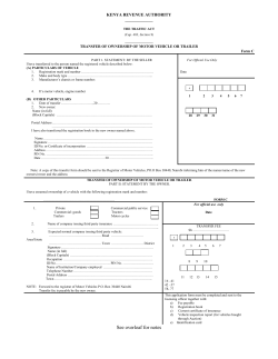


© Copyright 2026