
METAMODELS FOR COMPUTER-BASED ENGINEERING DESIGN
METAMODELS FOR COMPUTER-BASED ENGINEERING DESIGN: SURVEY AND
RECOMMENDATIONS
Timothy W. Simpson<, Jesse Peplinski; , Patrick N. KochH, and Janet K. Allen†
Systems Realization Laboratory
Woodruff School of Mechanical Engineering
Georgia Institute of Technology
Atlanta, Georgia 30332-0405, USA
ABSTRACT
The use of statistical techniques to build approximations of expensive computer analysis codes
pervades much of today’s engineering design. These statistical approximations, or metamodels,
are used to replace the actual expensive computer analyses, facilitating multidisciplinary,
multiobjective optimization and concept exploration. In this paper we review several of these
techniques including design of experiments, response surface methodology, Taguchi methods,
neural networks, inductive learning, and kriging.
We survey their existing application in
engineering design and then address the dangers of applying traditional statistical techniques to
approximate deterministic computer analysis codes. We conclude with recommendations for the
appropriate use of statistical approximation techniques in given situations and how common
pitfalls can be avoided.
1 INTRODUCTION
Much of today's engineering analysis consists of running complex computer codes: supplying
a vector of design variables (inputs) x and computing a vector of responses (outputs) y. Despite
steady advances in computing power, the expense of running many analysis codes remains nontrivial; single evaluations of aerodynamic or finite-element analyses can take minutes to hours, if
<
Currently Assistant Professor of Mechanical & Nuclear Engineering and Industrial & Manufacturing Engineering, The Pennsylvania State
University, University Park, PA.
Currently Associated with The General Electric Corporation, Schennectedy NY.
H
Currently at Engineous Software, Inc. Cary, NC.
;
.
not longer. Moreover, this mode of query-and-response often leads to a trial and error approach
to design whereby a designer may never uncover the functional relationship between x and y and
therefore never identify the "best" settings for input values.
Statistical techniques are widely used in engineering design to address these concerns. The
basic approach is to construct approximations of the analysis codes that are more efficient to run
and yield insight into the functional relationship between x and y. If the true nature of a computer
analysis code is
y = f(x),
then a "model of the model" or metamodel (Kleijnen, 1987) of the original analysis code is
yˆ
= g(x), and so y = yˆ + ε
where ε represents both the error of approximation and measurement (random) errors. The most
common metamodeling approach is to apply the design of experiments (DOE) to identify an
efficient set of computer runs (x1, x2, ..., xn) and then use regression analysis to create a
polynomial approximation of the computer analysis code. These approximations then can replace
the existing analysis code while providing:
• a better understanding of the relationship between x and y,
• easier integration of domain dependent computer codes, and
• fast analysis tools for optimization and exploration of the design space by using
approximations in lieu of the computationally expensive analysis codes themselves.
We have found that many applications (including our own) using these methods for computerbased design are statistically questionable because many analysis codes are deterministic in which
the error of approximation is not due to random effects. This calls into question the subsequent
†
Corresponding author. Email: [email protected]. Phone/Fax: 404-894-8168/9342.
2
statistical analyses of model significance. Consequently, we seek to highlight potential statistical
pitfalls in metamodeling and provide specific recommendations for the proper use of
metamodeling techniques in deterministic computer-based engineering design. In Section 2 we
present a review of metamodeling techniques including regression analysis, neural networks,
inductive learning, and kriging. We conclude Section 2 with an introduction to the general
statistical approaches of response surface methodology and Taguchi's robust design. In Section 3
we describe the engineering design context for statistical applications, review existing applications
and methods and conclude with a closer look at deterministic applications of metamodeling. In
Section 4 we present some recommendations for avoiding pitfalls in using metamodeling, and in
Section 5 we conclude by discussing some more advanced issues that contribute to making
metamodeling an active and interesting research area.
2 REVIEW OF METAMODELING TECHNIQUES
Metamodeling involves (a) choosing an experimental design for generating data, (b) choosing
a model to represent the data, and then (c) fitting the model to the observed data. There are
several options for each of these steps as shown in Figure 1, and we have attempted to highlight a
few of the more prevalent ones. For example, building a neural network involves fitting a
network of neurons by means of backpropagation to data which is typically hand selected while
Response Surface Methodology usually employs central composite designs, second order
polynomials and least squares regression analysis.
3
EXPERIMENTAL
DESIGN
MODEL
CHOICE
MODEL
FITTING
SAMPLE
APPROXIMATION
TECHNIQUES
(Fractional)
Factorial
Polynomial
(linear, quadratic)
Least Squares
Regression
Response Surface
Methodology
Central Composite
Splines
(linear, cubic)
Weighted
Least Squares
Regression
Box-Behnken
D-Optimal
G-Optimal
Realization of a
Stochastic Process
Orthogonal Array
Kernel Smoothing
Plackett-Burman
Hexagon
Hybrid
Latin Hypercube
Select By Hand
Random Selection
Radial Basis
Functions
Best Linear
Unbiased Predictor
Kriging
Best Linear
Predictor
Log-Likelihood
Network of
Neurons
Backpropagation
Neural
Networks
Rulebase or
Decision Tree
Entropy
(info.-theoretic)
Inductive
Learning
Figure 1. Techniques for Metamodeling
In the remainder of this section we provide a brief overview of several of the options listed in
Figure 1. In Section 2.1 the focus is on experimental designs, particularly (fractional) factorial
designs, central composite designs and orthogonal arrays. In Section 2.2 we discuss model choice
and model fitting, focusing on response surfaces, neural networks, inductive learning and kriging.
We conclude with an overview of two of the more common metamodeling techniques, namely,
response surface methodology and Taguchi's robust design.
2.1
Experimental Design
Properly designed experiments are essential for effective computer utilization. In engineering,
traditionally a single parameter is varied (perturbed) and the effects are observed. Alternatively,
combinations of factor settings are assigned either systematically (e.g., grid search) or randomly
to provide an alternative for comparison. Experimental design techniques that were originally
developed for physical experiments are being applied to the design of computer experiments to
4
increase the efficiency of these analyses.
In this section an overview of different types of
experiment designs is provided along with measures of merit for selecting/comparing different
experimental designs.
2.1.1 A Survey of Experimental Designs. An experimental design represents a sequence of
experiments to be performed, expressed in terms of factors (design variables) set at specified
levels (predefined values). An experimental design is represented by a matrix, X, where the rows
denote experiment runs, and the columns denote particular factor settings.
Factorial Designs: The most basic experimental design is a full factorial design. The number
of design points dictated by a full factorial design is the product of the number of levels for each
factor. The most common are 2k (for evaluating main effects and interactions) and 3k designs (for
evaluating main and quadratic effects and interactions) for k factors at 2 and 3 levels, respectively.
A 23 full factorial design is shown in Figure 2(a).
The size of a full factorial experiment increases exponentially with the number of factors; this
leads to an unmanageable number of experiments. Fractional factorial designs are used when
experiments are costly and many factors are required. A fractional factorial design is a fraction of
a full factorial design; the most common are 2(k-p) designs in which the fraction is 1/2(p). A half
fraction of the 23 full factorial design is shown in Figure 2(b). The reduction of the number of
design points in a fractional factorial design is not without a price. The 23 full factorial design
shown in Figure 2(a) allows estimation of all main effects (x1, x2, x3), all two factor interactions
(x1x2, x1x3 and x2x3), as well as the three factor interaction (x1x2x3). For the 23-1 fractional
factorial indicated by the solid dots in Figure 2(b), the main effects are aliased (or biased) with the
two factor interactions. Aliased effects cannot be estimated independently unless they are known
(or assumed) not to exist.
5
X2
X2
X2
X1
X3
X1
X1
X3
X3
(a) 23 Full Factorial (b) 23-1 Fractional Factorial
(c) Composite Design
Figure 2. Basic Three-Factor Designs
Often 2k and 2(k-p) designs are used to identify or screen for important factors. When there
are many factors, the sparsity of effects principle (Montgomery, 1997) can be invoked whereby
the system is assumed to be dominated by main effects and low order interactions. Thus, two
level fractional factorial designs are used to "screen" factors to identify those with the greatest
effects. The sparsity of effects principle is not always valid, however; Hunter, 1985, notes that
every design provides aliased estimates: quadratic and cubic effects, if present, bias the estimates
of the mean and main effects when a two level fractional factorial design is used.
One specific family of fractional factorial designs frequently used for screening are two level
Plackett-Burman (PB) designs (Plackett and Burman, 1946). These are used to study k=n-1
factors in n=4m design points, where m is an integer. PB designs in which n is a power of two are
called geometric designs and are identical to 2(k-p) fractional factorials. If n is strictly a multiple of
four, the PB designs are referred to as non-geometric designs and have very messy alias
structures. Their use in practical problems is problematic particularly if the design is saturated
(i.e., the number of factors is exactly n-1). If interactions are negligible, however, these designs
allow unbiased estimation of all main effects, and require only one more design point than the
number of factors; they also give the smallest possible variance (Box, et al., 1978). Myers and
Montgomery(1995) present a more complete discussion of factorial designs and aliasing of
effects. Minimum variance and minimum size designs are discussed in Section 2.1.2.
6
Central Composite and Box-Behnken Designs: To estimate quadratic effects, 3k or 3(k-p)
designs can be used but often require an unmanageable number of design points. The most
common second order designs, configured to reduce the number of design points, are central
composite and Box-Behnken designs.
A central composite design (CCD) is a two level (2(k-p) or 2k) factorial design, augmented by
n0 center points and two "star" points positioned at ±α for each factor. This design, shown for
three factors in Figure 2(c), consists of 2(k-p)+2k+no total design points to estimate 2k+k(k-1)/2+1
coefficients. For three factors, setting α=1 locates the star points on the centers of the faces of
the cube, giving a face-centered central composite (CCF) design; note that for values of α other
than 1, each factor is evaluated at five levels.
Often it is desirable to use the smallest number of factor levels in an experimental design. One
common class of such designs is the Box-Behnken designs (Box and Behnken, 1960). These are
formed by combining 2k factorials with incomplete block designs. They do not contain points at
the vertices of the hypercube defined by the upper and lower limits for each factor. This is
desirable if these extreme points are expensive or impossible to test. More information about
CCD and Box-Behnken designs can be found in (Montgomery, 1997).
Orthogonal Arrays: The experiment designs used by Taguchi, orthogonal arrays, are usually
simply fractional factorial designs in two or three levels (2(k-p) and 3(k-p) designs). These arrays are
constructed to reduce the number of design points necessary; two-level L4, L12, and L16 arrays, for
example, allow 3, 11, and 15 factors/effects to be evaluated with 4, 12, and 16 design points,
respectively. Often these designs are identical to Plackett-Burman designs (Lucas, 1994). The
definition of orthogonality for these arrays and other experiment designs is given in Section 2.1.2.
An overview of Taguchi's approach to parameter design is given in Section 2.3.
7
“Space Filling” Designs: For sampling deterministic computer experiments, many researchers
advocate the use of “space filling” designs which treat all regions of the design space equally.
Simpson (1998) and Palmer (1998) also recommend the use of space filling designs in the early
stages of design when the form of the metamodel cannot be pre-specified. As discussed by
Booker, et al.(1995), in the "classical" design and analysis of physical experiments (i.e., using
central composite and factorial designs), random variation is accounted for by spreading the
sample points out in the design space and by taking multiple data points (replicates), see Figure 3.
Sacks, et al. (1989) state that the “classical” notions of experimental blocking, replication, and
randomization are irrelevant when it comes to deterministic computer experiments; thus, sample
points in DACE should be chosen to fill the design space. They suggest minimizing the integrated
mean squared error (IMSE) over the design region by using IMSE-optimal designs; the “space
filling” design illustrated in Figure 3(b) is an IMSE optimal design.
1.0
1.0
0.5
0.5
x2 0.0
x2 0.0
-0.5
-0.5
-1.0
-1.0
-1.0
-0.5
0.0
0.5
-1.0
1.0
-0.5
0.0
0.5
x1
x1
(a) “Classical”Design
(b) “Space Filling”Design
1.0
Figure 3. “Classical” and “Space Filling” Designs [adapted from Booker, et al., 1995]
Koch (1997) investigates the use of a modified central composite design which combines half
fractions of a CCI and a CCF to more evenly distribute the points throughout the design space.
Koehler and Owen (1996) describe several Bayesian and Frequentist “space filling” designs,
including maximum entropy designs, mean squared-error designs, minimax and maximin designs,
8
Latin hypercubes, randomized orthogonal arrays, and scrambled nets. Minimax and maximin
designs were originally proposed by Johnson, et al.(1990) specifically for use with computer
experiments. Sherwy and Wynn (1988) and Currin, et al. (1991) use the maximum entropy
principle to develop designs for computer experiments. Tang (1993) describes orthogonal arraybased Latin hypercubes which he asserts are more suitable for computer experiments than general
Latin hypercubes.
Park (1994) discusses optimal Latin hypercube designs for computer
experiments which either minimize IMSE or maximize entropy, spreading the points out over the
design region. Morris and Mitchell (1995) propose maximin distance designs found within the
class of Latin hypercube arrangements since they “offer a compromise between the
entropy/maximin criterion, and good projective properties in each dimension.” Owen (1992)
advocates the use of orthogonal arrays as suitable designs for computer experiments, numerical
integration, and visualization; a collection of orthogonal array generators is available over the
Internet (Owen, 1995). A review of Bayesian experimental designs for linear and nonlinear
regression models is given in Chaloner and Verdinelli (1995_.
2.1.2 Measures of Merit for Evaluating Experimental Designs. Selecting the appropriate design is
essential for effective experimentation: the desire to gain as much information as possible about
the response-factor relationships is balanced against the cost of experimentation.
Several
measures of merit are available and useful for evaluating and comparing experimental designs.
Orthogonality, Rotatability, Minimum Variance, and Minimum Bias: To facilitate efficient
estimates of parameters, four desirable characteristics of an experimental design are orthogonality,
rotatability, minimum variance, and minimum bias. A design is orthogonal if, for every pair of
factors xi and xj, the sum of the cross-products of the N design points:
9
N
∑x
iu
u =1
x ju
is zero. For a first order model, the estimates of all coefficients will have minimum variance if the
design can be configured so that
N
∑x
u =1
2
iu
=N;
the variance of predictions yˆ will also have constant variance at a fixed distance from the center
of the design, and the design will also be rotatable.
In second order modeling, Hunter (1985) suggests that orthogonality is less important: "If the
objective of the experimenter is to forecast a response at either present or future settings of x,
then an unbiased minimum variance estimate of the forecast yˆ is required. In the late 1950's Box
and his co-workers demonstrated that “rotatability...and the minimization of bias from higher
order terms...were the essential criteria for good forecasting."
A design is rotatable if
N•Var[ yˆ (x)]/σ2 has the same value at any two locations that are the same distance from the
design center. The requirements for minimum variance and minimum bias designs for second
order models are beyond the scope of this work; we refer the reader to (Myers and Montgomery,
1995) for more information.
Unsaturated/Saturated and Supersaturated Designs: In many cases, the primary concern in
the design of an experiment is its size. Most designs are unsaturated in that they contain at least
two more design points than the number of factors. A saturated design is one in which the
number of design points is equal to one more than the number of factor effects to be estimated.
Saturated fractional factorial designs allow unbiased estimation of all main effects with the
smallest possible variance and size (Box, Hunter et al., 1978). The most common examples of
saturated designs are the Plackett-Burman two level design and Taguchi’s orthogonal arrays. For
10
estimating second order effects, small composite designs have been developed to reduce the
number of required design points. A small composite design is saturated if the number of design
points is 2k+k(k-1)/2+1 (the number of coefficients to be estimated for a full quadratic model).
Myers and Montgomery(1995) note that recent work has suggested that these designs may not
always be good; additional comments on small composite designs can be found in Box and Draper
(1987) and Lucas (1974). Finally, in supersaturated designs the number of design points is less
than or equal to the number of factors (Draper and Lin, 1990).
It is most desirable to use unsaturated designs for predictive models, unless running the
necessary experiments is prohibitively expensive. When comparing experiments based on the
number of design points and the information obtained, the D-optimal and D-efficiency statistics
are often used.
D-optimal and D-efficiency: A design is said to be D-optimal if |X'X|/np is maximized where
X is the expanded design matrix which has n rows (one for each design setting) and p columns
(one column for each coefficient to be estimated plus one column for the overall mean). The Defficiency statistic for comparing designs, Eq. (1), compares a design against a D-optimal design,
normalized by the size of the matrix in order to compare designs of different sizes.
D-efficiency = (|X'X|design/|X'X|D-optimum)1/p
(1)
Other statistics for comparing designs such as G-efficiency, Q-efficiency, and A-optimality have
also been formulated, see (Myers and Montgomery, 1995). We now turn to the issues of model
choice and model fitting.
2.2
Model Choice and Model Fitting
After selecting an appropriate experimental design and performing the necessary computer
runs, the next step is to choose an approximating model and fitting method. Many alternative
11
models and methods exist, but here we review the four that are most prevalent in the literature:
response surfaces, neural networks, inductive learning, and kriging.
2.2.1 Response Surfaces. Given a response, y, and a vector of independent factors x influencing y,
the relationship between y and x is:
y = f(x) + ε ,
(2)
where ε represents random error which is assumed to be normally distributed with mean zero and
standard deviation σ. Since the true response surface function f(x) is usually unknown, a response
surface g(x) is created to approximate f(x). Predicted values are then obtained using yˆ = g(x).
The most widely used response surface approximating functions are low-order polynomials.
For low curvature, a first order polynomial can be used as in Eq. (3); for significant curvature, a
second order polynomial which includes all two-factor interactions is available, see Eq. (4).
yˆ = β0 +
yˆ = β0 +
k
∑
i =1
βi xi +
k
∑
i =1
k
∑ βx
(3)
i i
i =1
βii xi +
2
k
k
∑ ∑
i =1 j =1,i < j
βij xi x j
(4)
The parameters of the polynomials in Eq. (3) and Eq. (4) are usually determined by least
squares regression analysis by fitting the response surface approximations to existing data. These
approximations are normally used for prediction within response surface methodology (RSM).
RSM was first developed by Box and Wilson in1951. A more complete discussion of response
surfaces and least squares fitting is presented in (Myers and Montgomery, 1995). An overview of
RSM is given in Section 2.3.
2.2.2 Neural Networks. A neural network is composed of neurons (single-unit perceptrons) which
are multiple linear regression models with a nonlinear (typically sigmoidal) transformation on y. If
12
the inputs to each neuron are denoted {x1, x2, ..., xn}, and the regression coefficients are denoted
by the weights, wi, then the output, y, might be given by
y=
1
1 + e-η/T
(5)
where η = Σwixi + β (where β is the "bias value" of a neuron), and T is the slope parameter of the
sigmoid defined by the user. A neural network is then created by assembling the neurons into an
architecture; the most common of which is the multi-layer feedforward architecture, see Figure 4.
Inputs
x1
x2
w1
x3
•
•
wn
•
xn
Input
Units
Hidden
Layer
Output
Units
η = Σw ixi + β
Output
y
Neuron
y=
1
1 + e -η/T
(a) Single-Unit Perceptron
~x
~y
•
•
•
•
•
•
(b) Feedforward Two-layer Architecture
Figure 4. Typical Neuron and Architecture
There are two main issues in building a neural network: (1) specifying the architecture and (2)
training the neural network to perform well with reference to a training set. "To a statistician, this
is equivalent to (i) specifying a regression model, and (ii) estimating the parameters of the model
given a set of data" (Cheng and Titterington, 1994). If the architecture is made large enough, a
neural network can be a nearly universal approximator (Rumelhart, et al.,1994). Hajela and Berke
(1993) review the use of neural networks in structural analysis and design.
"Training" a neural network is the determination of the proper values for all weights, w i, in the
architecture and is usually done by backpropagation (Rumelhart, et al., 1994); this requires a set
13
of n training data points {(x1,y1), (x2,y2), ..., (xp,yp)}.
For a network with output y, the
performance is
E = ∑ ( y p − yˆp )
2
(6)
p
where yˆ p is the output that results from the network given input xp, and E is the total error of the
system. The weights are then adjusted in proportion to
∂E ∂y
.
∂y ∂wij
(7)
Neural networks are best suited for approximating deterministic functions in regression-type
applications. "In most applications of neural networks that generate regression-like output, there
is no explicit mention of randomness. Instead, the aim is function approximation” (Cheng and
Titterington, 1994). Typical applications of neural nets are speech recognition and handwritten
character recognition where the data is complex and of high dimensionality. Networks with tens
of thousands of parameters have been used but the requisite gathering of training data and
calculation of model parameters can be extremely computationally expensive.
Cheng and
Titterington (1994) comment that "...the procedure is to toss the data directly into the NN
software, use tens of thousands of parameters in the fit, let the workstation run 2-3 weeks
grinding away doing the gradient descent, and voilá, out comes the result." Rogers and LaMarsh
(1995) describe parallel computing efforts aimed at reducing the time required to “train” neural
networks.
2.2.3
Inductive Learning. Inductive learning is one of five main paradigms of machine learning
that also include neural networks, case-based learning, genetic algorithms, and analytic learning
(Langley and Simon, 1995). Of these five, inductive learning is the most akin to regression and
metamodeling and is therefore the focus here. An inductive learning system induces rules from
14
examples; the fundamental modeling constructs are condition-action rules which partition the data
into discrete categories and can be combined into decision trees for ease of interpretation, see
Figure 5.
y = f(x 1,x2)
x1, x2
x1 = a
x1 = b
x2 = c
x2 = d
x2 = e
x2 = f
y = y1
y = y2
y = y3
y = y4
Figure 5. A Decision Tree
Training data are required in the form {(x1,y1),(x2,y2), ..., (xn,yn)} where xi is a vector of
attribute values (e.g., processing parameters and environmental conditions), and each yi is a
corresponding observed output value. Although attributes and outputs can be real-valued, the
method is better suited to discrete-valued data; real values must often be transformed into discrete
representations (Evans and Fisher, 1994). Once the data has been collected, training algorithms
build a decision tree by selecting the "best" divisive attribute and then recursively calling the
resulting data subsets. Although trees can be built by selecting attributes randomly, it is more
efficient to select attributes that minimize the amount of information needed for category
membership. The mathematics of such an information-theoretic approach are given in (Evans and
Fischer, 1994).
15
Many of the applications of inductive learning have been in process control and diagnostic
systems, and inductive learning approaches can be used to automate the knowledge-acquisition
process of building expert systems. Furthermore, although decision trees appear best suited for
applications with discrete input and output values, there are also applications with continuous
variables that have met with greater success than standard statistical analysis. Leech (1986)
reports a process-control application where "Standard statistical analysis methods were employed
with limited success. Some of the data were non-numerical, the dependencies between variables
were not well understood, and it was necessary to simultaneously control several characteristics
of the final product while working within system constraints.
The results of the statistical
analysis, a set of correlations for each output of interest, were difficult for people responsible for
the day-to-day operation to interpret and use." Additional examples can be found in (Evans and
Fischer, 1994; Langley and Simon, 1995).
2.2.4 Kriging. Since many computer analysis codes are deterministic and therefore not subject to
measurement error, the usual measures of uncertainty derived from least-squares residuals have
no obvious meaning (cf., Sacks, et al., 1989). Consequently, some statisticians (e.g., Sacks, et al.,
1989; Welch, et al., 1992; Koehler, 1996, Booker, et al., 1995) have suggested modeling
responses as a combination of a polynomial model plus departures of the form:
y(x) = f(x) + Z(x)
(8)
where y(x) is the unknown function of interest, f(x) is a known polynomial function of x, and Z(x)
is the realization of a normally distributed Gaussian random process with mean zero, variance σ2,
and non-zero covariance. The f(x) term in Eq. (8) is similar to the polynomial model in a
response surface and provides a "global" model of the design space; in many cases f(x) is simply
taken to be a constant term, see (Sacks, et al., 1992; Welch et al., 1989, Welch, et al., 1992).
16
While f(x) "globally" approximates the design space, Z(x) creates "localized" deviations so
that the kriging model interpolates the ns sampled data points. The covariance matrix of Z(x) is
given by:
Cov[Z(xi),Z(xj)] = σ2 R([R(xi,xj)].
(9)
where R is the correlation matrix, and R(xi,xj) is the correlation function between any two of the
ns sampled data points xi and xj. R is a (ns x ns) symmetric matrix with ones along the diagonal.
The correlation function R(xi,xj) is specified by the user; Sacks, et al. (1989) and Koehler and
Owen (1996) discuss several correlation functions which may be used. A Gaussian correlation
function of the form:
R (x i ,x j ) = exp[−
∑ k=1 θk xik −
ns
2
x jk ]
(10)
is the most frequently used where θk are the unknown correlation parameters used to fit the
model, and the xki and xkj are the kth components of sample points xi and xj. In some cases using
a single correlation parameter gives sufficiently good results, see (Osio and Amon, 1996; Sacks,
et al., 1989).
Predicted estimates, yˆ (x), of the response y(x) at untried values of x are given by:
ˆ)
yˆ = βˆ + r T (x)R − 1 (y − fβ
(11)
where y is the column vector of length ns which contains the values of the response at each sample
point, and f is a column vector of length ns which is filled with ones when f(x) is taken as a
constant. In Eq. (11), rT(x) is the correlation vector of length ns between an untried x and the
sampled data points {x1, x2, ..., xns} and is given by:
rT(x) = [R(x,x1), R(x,x2), ..., R(x,xns)]T
17
(12)
ˆ is estimated using Eq. (13).
In Eq. (11), β
ˆ = (f T R − 1 f )− 1 f T R − 1y .
β
(13)
ˆ2 , from the underlying global model (not the variance in the
The estimate of the variance, σ
observed data) is given by
ˆT −1
ˆ
ˆ2 = (y − fβ) R (y − fβ)
σ
ns
(14)
ˆ. The maximum likelihood estimates (i.e., "best
where f(x) is assumed to be the constant β
guesses") for the θk in Eq. (10) used to fit the model are found by maximizing (Booker, et al.,
1995):
−
ˆ2 ) + ln|R| ]
[n s ln(σ
2
(15)
ˆ2 and |R| are both functions of θk. While any values for the θk create an
for θk > 0 where both σ
interpolative approximation model, the “best” kriging model is found by maximizing Eq. (15).
Depending on the choice of correlation function in Eq. (10), kriging can either "honor the
data," providing an exact interpolation of the data, or "smooth the data," providing an inexact
interpolation (Cressie, 1998). Finally, it should be noted that kriging is different from fitting
splines (i.e., non-parametric regression models). In several comparative studies kriging performs
as well as, if not better than, splines (Laslett, 1994).
2.2.4 Additional Metamodeling Approaches. For completeness, we include references for some
alternative metamodeling techniques that have not been discussed in the previous subsections.
Rasmussen (1990) offers an accumulated approximation technique for structural optimization
which refines the approximation of objective and constraint functions by accumulating the
18
function values of previously visited points.
Similarly, Balling and Clark (1992) describe
weighted and gradient-based approximations for use with optimization which utilize weighted
sums of exact function values at sample points. Friedman (1991) describes multivariate adaptive
regression splines: a flexible regression modeling method based on recursive partitioning and
spline fitting for high dimensional data. Dyn, et al. (1986) use radial basis functions to build
global approximation surfaces to interpolate smooth data.
Wang, et al. (1996) present
multivariate Hermite approximations for multidisciplinary design optimization which uses data
generated during the course of iterative optimization; it is compared against linear, reciprocal, and
other standard approximations but shows inefficiencies because it requires more data points.
Wavelet modeling uses a special form of a basis function which is especially effective in modeling
sharp jumps in a response surface (Mallet, 1998).
Finally, Friedman and Steutzle (1981)
introduce projection pursuit regression which works well in high-dimensional (< 50) data and with
large data sets (can handle 200,000+ data points). Project pursuit regression takes the data and
generates different projections of it along linear combinations of the variables; an optimizer finds
the best projections and builds a predictor by summing them together with arbitrary levels of
precision.
This concludes our discussion on experimental design, model selection and model fitting. We
now turn to more general methods for experimental design and modeling building.
2.3
Experimentation and Metamodeling Strategies
Two widely used methods incorporating experimental design, model building, and prediction
are response surface methodology and Taguchi's robust design or parameter design. A brief
overview of these two approaches is provided.
19
2.3.1
Response Surface Methodology (RSM). Different authors describe RSM differently.
Myers, et al.(1989) define RSM as "a collection of tools in design or data analysis that enhance
the exploration of a region of design variables in one or more responses." Box and Draper (1987)
state that, "Response surface methodology comprises a group of statistical techniques for
empirical model building and model exploitation. By careful design and analysis of experiments, it
seeks to relate a response, or output variable, to the levels of a number of predictors, or input
variables, that affect it." Finally, Myers and Montgomery (1995) state that RSM “is a collection
of statistical and mathematical techniques useful for developing, improving, and optimizing
process. It also has important applications in the design, development, and formulation of new
products, as well as in the improvement of existing product designs.”
The “collection of statistical and mathematical techniques” of which these authors speak refers
to the design of experiments (Section 2.1), least squares regression analysis and response surface
model building (Section 2.2.1), and "model exploitation," exploring a factor space seeking
optimum factor settings. The general RSM approach includes all or some of the following steps:
i) screening: when the number of factors is large or when experimentation is expensive,
screening experiments are used to reduce the set of factors to those that are most influential to
the response(s) being investigated;
ii) first order experimentation: when the starting point is far from the optimum point or when
knowledge about the space being investigated is sought, first order models and an approach
such as steepest ascent are used to "rapidly and economically move to the vicinity of the
optimum" (Montgomery, 1997);
iii) second order experimentation: after the best solution using first order methods is obtained, a
second order model is fit in the region of the first order solution to evaluate curvature effects
and to attempt to improve the solution.
20
Response surfaces are typically second-order polynomial models; therefore, they have limited
capability to model accurately non-linear functions of arbitrary shape. Obviously, higher-order
response surfaces can be used to model a non-linear design space; however, instabilities may arise
(cf. Barton, 1992) or what is more likely to happen is that it is difficult to take enough sample
points in order to estimate all of the coefficients in the polynomial equation, particularly in high
dimensions. Hence, many researchers advocate the use of a sequential response surface modeling
approach using move limits ( e.g., Toporov, et al., 1996 and Wujek, 1997) or a trust region
approach ( e.g., Rodriguez, et al., 1997 and Wujek and Renaud, 1998).
A more detailed description of RSM techniques and tools can be found in (Myers and
Montgomery, 1995) and a comprehensive review of RSM developments and applications from
1966-1988 is given in (Myers, et al, 1989). In Section 3 we review recent applications in
aerospace and mechanical engineering design, but first we discuss Taguchi’s robust design
approach.
2.3.3
Taguchi's Robust Design. Genichi Taguchi developed an approach for industrial product
design built on statistically designed experiments. Taguchi's robust design for quality engineering
includes three steps: system design, parameter design, and tolerance design (Byrne and Taguchi,
1987). The key step is parameter design within which statistical experimentation is incorporated.
Rather than simply improving or optimizing a response value, the focus in parameter design is
to identify factor settings that minimize variation in performance and adjust the mean performance
to a desired target in order to minimize the associated loss. Factors included in experimentation
include control factors and noise factors; control factors are set and held at specific values, while
noise factors cannot be controlled, e.g., shop floor temperature.
The evaluation of mean
performance and performance variation is accomplished by "crossing" two orthogonal arrays
21
(Section 2.1.1). Control factors are varied according to an inner array, or "control", array, and
for each run of the control array, noise factors are varied according to an outer, or "noise", array.
For each control factor experiment, a response value is obtained for each noise factor design
point. The mean and variance of the response (measured across the noise design points) are
calculated. The performance characteristic used by Taguchi is a signal-to-noise (S/N) ratio
defined in terms of the mean and variance of the response. Several alternate S/N ratios are
available based on whether lower, higher, or nominal response values are desired, see (Ross,
1996).
The Taguchi approach does not explicitly include model building and optimization. Analysis
of experimental results is used to identify factor effects, to plan additional experiments, and to set
factor values for improved performance. A comprehensive discussion of the Taguchi approach is
given in (Ross, 1996; Phadke, 1989). Taguchi methods have been used extensively in engineering
design and are often incorporated within traditional RSM for efficient, effective, and robust design
(Myers and Montgomery, 1995). These applications and their implications for engineering design
are discussed next.
3 METAMODELING IN ENGINEERING DESIGN
How are the metamodeling techniques of the previous section employed in engineering
design? All of these techniques can be used to create approximations of existing computer
analyses, and produce fast analysis modules for more efficient computation. These metamodeling
techniques also yield insight into the functional relationship between input and output parameters.
Where would such models be useful?
A designer's goal is usually to arrive at improved or
robust solutions that are the values of design variables that best meet the design objectives as
shown in Figure 6. A search for these solutions usually relies on an optimization technique that
22
generates and evaluates many potential solutions in the path toward design improvement; thus,
fast analysis modules are an imperative.
When are metamodels useful or appropriate? In the later stages of design when detailed
information about specific solutions is available, highly accurate analysis is essential. In the early
stages of design, however, the focus is on generating, evaluating, and comparing potential
conceptual configurations. The early stages of design are characterized by a large amount of
information, often uncertain, which must be managed. To ensure the identification of a "good"
system configuration, a comprehensive search is necessary. In this case, the tradeoff between
accuracy and efficiency may be appropriate. The creation of metamodels allows fast analysis,
facilitating both comprehensive and efficient design space search at the expense of a (hopefully
slight) loss of accuracy.
23
Given:
Factors,
Responses
Large # of
Factors?
YES
Run Screening
Experiment
Screening
NO
Run Modeling
Experiment(s)
Model
Building
Reduce #
Factors
Build Predictive
Model ( y )
Noise
Factors?
YES
Build Robustness
Model ( µy , σy )
NO
Model
Exercising
Search Design
Space
Solutions
(improved or robust)
Figure 6. Principal Use of Statistics in Computer-Based Design
Having established context for using metamodels in engineering design, we present a review
of several statistical applications in engineering design in Section 3.1. In Section 3.2 we discuss
general metamodel-based methods that have been developed for engineering applications, and we
conclude by discussing some of the pitfalls associated with the application of statistical techniques
to deterministic computer experiments in Section 3.3. This paves the way for Section 4 wherein
guidelines for the appropriate use of metamodels in computer-based design are discussed.
24
3.1
Applications in Engineering Design
3.1.1
DOE, RSM, and Taguchi’s Robust Design. In Table 1 we present a survey of several
engineering applications of design of experiments, response surface methodology, and Taguchi's
robust design approach.
Most of these examples come from aerospace and mechanical
engineering design applications presented at conferences in recent years.
A review of
approximation concepts used in structural design can be found in (Barthelemy and Haftka, 1993).
Some observations regarding our findings are as follows.
• Central composite designs and D-optimal designs seem to be preferred among aerospace
engineers while orthogonal arrays (OAs) are preferred by mechanical engineers; grid and
random point searches are seldom used since they are less efficient.
• Optimization seems to be the principal driver for aerospace applications of DOE and RSM;
these types of applications typically involve the use of computer intensive analysis and
optimization routines, and DOE and RSM is a logical choice for increased efficiency.
• Mechanical engineers usually use OAs and Taguchi's approach for robust design and the signalto-noise ratio for parameter and tolerance design.
• Very few designers actually model Taguchi's loss function directly (e.g., Beard and Sutherland,
1993); many prefer to model the response instead.
• Most applications use second order response surface models; there are only a few cases where
higher order (e.g., Venter, et al., 1996) and mixed polynomial models (e.g., Roux, et al., 1996)
are used for engineering design.
• When orthogonal arrays are used, special care must be taken to avoid aliasing main effects with
interactions, unless the interactions are known (or assumed) to be insignificant.
25
• Most applications utilize least squares regression analysis when fitting a model; only a few use
stepwise regression, and this is usually because the model is not second order.
Table 1. Survey of Engineering Applications of DOE, RSM, and Taguchi's Robust Design
(Simpson, et al., 1997)
3.1.1
Kriging Applications. Kriging, also referred to as DACE (Design and Analysis of
Computer Experiments) after the paper (Sacks, et al., 1989), has found limited use in engineering
26
design and optimization. This may be due to the lack of readily available software to fit kriging
models, the added complexity of fitting a kriging model, or the additional effort required to use a
kriging model. Simpson, et al. (1997) detail a preliminary comparison of second-order response
surface models and kriging models for the multidisciplinary design of an aerospike nozzle which
has three geometry (design) variables; neither the kriging models nor the response surface models
consistently outperform the other in this engineering example.
Giunta (1997) presents an
investigation into the use of kriging for the multidisciplinary design optimization of a High Speed
Civil Transport aircraft. He explores a five and a ten variable design problem, observing that the
kriging and response surface modeling approaches yield similar results due to the quadratic trend
of the responses. Osio and Amon(1996) have developed an extension of DACE modeling for
numerical optimization which uses a multistage strategy for refining the accuracy of the model;
they have applied their approach to the thermal design of an embedded electronic package which
has 5 design variables. Booker, et al. (1996) solve a 31 variable helicopter rotor structural design
problem using an similar approximation methodology based on kriging. Booker (1996) extends
the helicopter rotor design problem to include 56 structural variables to examine the aeroelastic
and dynamic response of the rotor. Welch, et al.(1992) describe a kriging-based approximation
methodology to identify important variables, detect curvature and interactions, and produce a
useful approximation model for two 20 variable problems using only 30-50 runs of the computer
code; they claim their method can cope with up to 30-40 variables provided factor sparsity can be
exploited. Trosset and Torczon (1997) have developed a numerical optimization strategy which
incorporates DACE modeling and pattern search methods for global optimization. Cox and John
(1995) have developed the Sequential Design for Optimization method which uses lower
confidence bounds on predicted values of the response for the sequential selection of evaluation
27
points during optimization.
Both approaches have shown improvements over traditional
optimization approaches when applied to a variety of standard mathematical test problems.
3.2
Existing Methods and Tools in Engineering Design
In this section we present some methods and tools developed specifically for engineering
which incorporate statistical techniques from Section 2. Since the Taguchi approach and RSM
have been widely applied in engineering design, a literature review comparing these approaches is
given first. This is followed by an overview of some methods and “tools” that have been
developed for general design applications.
These include the Robust Concept Exploration
Method, the Variable-Complexity Response Surface Modeling Method, and Concurrent
SubSpace Optimization to name a few.
3.2.1 Taguchi Approach vs. RSM. The Taguchi approach and RSM have been applied extensively
in engineering design. It is commonly accepted that the principles associated with the Taguchi
approach are both useful and very appropriate for industrial product design. Ramberg, et al.,
1991, suggest that "the loss function and the associated robust design philosophy provide fresh
insight into the process of optimizing or improving the simulation's performance." Two aspects of
the Taguchi approach are often criticized: the choice of experimental design (orthogonal arrays,
inner and outer) and the loss function (signal-to-noise ratio).
It has been argued and
demonstrated that the use of a single experiment combining control and noise factors is more
efficient, (Shoemaker, et al., 1991, Unal, et al., 1994; and Welch, et al., 1990). The drawbacks of
combining response mean and variance into a single loss function (signal-to-noise ratio) are welldocumented. Many authors advocate measuring the response directly and separately tracking
mean and variance (cf., Chen, et al., 1997; Ramberg, et al. 1991; Welch, et al., 1990). However,
28
Shoemaker, et al. (1991) warn that a "potential drawback of the response-model approach is that
it depends more critically than the loss-model approach on how well the model fits."
Given the wide acceptance of Taguchi robust design principles and the criticisms, many
advocate a combined Taguchi-RSM approach or simply using traditional RSM techniques within
the Taguchi framework, (Lucas, 1994; Myers, et al, 1989; Meyers and Montgomery, 1995; and
Ramberg, et al., 1991). We believe that orthogonal inner and outer arrays, and single composite
experiments each have advantages and disadvantages and appropriate uses, and that separate
observation of mean and variance leads to useful insight. Regardless, the core principles of both
Taguchi and RSM provide a foundation for many of the specific design methods discussed in
Section 3.2.2.
3.2.2 An Overview of Existing Methods.
The Robust Concept Exploration Method (RCEM)
facilitates quick evaluation of different design alternatives and generation of top-level design
specifications in the early stages of design (Chen et al., 1994; Chen et al, 1996). Foundational to
the RCEM is the integration of robust design principles, DOE, RSM, and the compromise
Decision Support Problem (a multiobjective decision model). The RCEM has been applied to the
multiobjective design of a High Speed Civil Transport (Chen et al., 1997 and Chen, et al., 1996),
a family of General Aviation Aircraft (Simpson, et al., 1996), a turbine lift engine (Koch, et al,
1996), a solar-powered irrigation system (Chen, et al., 1996), a flywheel (Lautenschlager, et al.,
1997), to manufacturing simulation (Peplinski, et al, 1996) and to maintainability design of aircraft
engines (Nottingham, et al., 1997). A preliminary investigation into the use of DOE and neural
networks to augment the capabilities of response surface modeling within the RCEM is given in
(Chen, et al., 1997).
29
The Variable-Complexity Response Surface Modeling (VCRSM) Method uses analyses of
varying fidelity to reduce the design space to the region of interest and build response surface
models of increasing accuracy (e.g., Giunta, et al., 1995 and Giunta, et al., 1994). The VCRSM
method employs DOE and RS modeling techniques and has been successfully applied to the
multidisciplinary wing design of a high speed civil transport (e.g., Balabanov, Kaufman, Giunta, et
al.,1996 and Balabanov, Kaufman, Knill et al, 1996; Giunta, et al, 1994; Kaufman, et al, 1996), to
the analysis and design of composite curved channel frames (Mason, et al., 1994), to the
structural design of bar trusses (Roux, et al., 1996), to predict the fatigue life of structures
(Venter, et al., 1997), to reduce numerical noise inherent in structural analyses (Giunta, et al,
1994 and Venter, et al., 1996) and shape design problems using fluid flow analysis (Narducci, et
al., 1995,), and to facilitate the integration of local and global analyses for structural optimization
(Gangadharan, et al., 1995; Ragon, et al., 1997; and Venkatraman, et al., 1997). Coarse-grained
parallelization of analysis codes for efficient response surface generation has also been
investigated (Burgee, et al, 1995; and Kaufman, et al., 1996).
Concurrent SubSpace Optimization (CSSO) uses data generated during concurrent subspace
optimizations to develop response surface approximations of the design space. Optimization of
these response surfaces forms the basis for the subspace coordination procedure. The data
generated by the subspace optimizers is not uniformly centered about the current design as in
CCD or other sampling strategies, but instead follows the descent path of the subspace
optimizers.
In (Renaud and Gabriele, 1994; Renaud and Gabriele, 1993; and Renaud and
Gabriele, 1991), interpolating polynomial response surfaces are constructed which have either a
first or second order basis for use in the CSSO coordination procedure. In (Wujek, et al., 1996),
a modified decomposition strategy is used to develop quadratic response surfaces for use in the
CSSO coordination procedure. Finally, in (Sellar and Batill, 1996; Sellar, Stelmack, et al., 1996;
30
and Sellar, Batill, et al, 1996), artificial neural network response surfaces are developed for use in
the CSSO coordination procedure.
Robust Design Simulation (RDS) is a stochastic approach which employs the principles of
Integrated Product and Process Development (IPPD) for the purpose of determining the optimum
values of design factors and proposed technologies (in the presence of uncertainty) which yield
affordable designs with low variability. Toward this end, RDS combines design of experiments
and response surface metamodels with Monte Carlo simulation and Fast Probability Techniques
(e.g., (Bandte and Mavris, 1997)) to achieve customer satisfaction through robust systems design
(Mavris, Bandte et al., 1995). RDS has been applied to the design of a High Speed Civil
Transport aircraft (Mavris, et al., 1996, Mavris, et al., 1995) and very large transports (Mavris,
Mantis, et al., 1997). RDS has also been used to study the economic uncertainty of the HSCT
(Mavris, Bandte and Schrage, 1997), and the feasibility/viability of aircraft (Mavris, et al., 1998).
NORMAN/DEBORA is a Technology Computer Aided Design system incorporating advanced
sequential DOE and RSM techniques to aid in engineering optimization and robust design
(Cartuyvels and Dupas, 1993). NORMAN/DEBORA includes a novel design of experiments
concept— Target
Oriented
Design— a
unique
parameter
transformation
technique—
RATIOFIND— and a non-linear, constrained optimizer— DEBORA (Cartuyvels and Dupas,
1993).
It has been successfully employed for semiconductor integrated circuit design and
optimization (Cartuyvels, et al., 1991; Cartyuvels, et al., 1992; Cartuyvels, et al, 1993, Huizing, et
al, 1995). An updated and more powerful version of NORMAN/DEBORA is being offered as
LMS Optimus (LMS Numerical Technologies, 1997).
The Probabilistic Design System (PDS) being developed at Pratt and Whitney uses BoxBehnken designs and response surface methodology to perform probabilistic design analysis of
gas turbine rotors (Fox, 1993; Fox, 1994). Fox (1996) describes twelve criteria which are used
31
to validate the response surfaces which are used in combination with cheap-to-run analyses in a
Monte Carlo Simulator to estimate the corresponding distributions of the responses and minimum
life of system components.
Adamson (1994) describes issues involved with developing,
calibrating, using, and testing the PDS and discusses Pratt and Whitney’s plans to validate the
PDS by designing, building, and testing actual parts.
DOE/Opt is a prototype computer system for DOE, RSM, and optimization (Boning and
Mozumder, 1994).
It has been used in semiconductor process/device design including
process/device optimization, simulator tuning, process control recipe generation, and design for
manufacturability.
Hierarchical and Interactive Decision Refinement (HIDER) is a methodology for concept
exploration in the early stages of design.
It integrates simulation, optimization, statistical
techniques, and machine learning to support design decision making, Reddy, 1996; and
Yerramareddy, 1992. The methodology is used to hierarchically refine/reduce “a large initial
design space through a series of multiple-objective optimizations, until a fully specified design is
obtained” (Yerramareddy and Lu, 1993). HIDER uses the Adaptive Interactive Modeling System
(AIMS) (Lu and Tcheng, 1991) to decompose the design space using distance-based, populationbased, and hyperplane-based algorithms. HIDER and AIMS have been applied to the design of a
cutting process (Lu and Tcheng, 1991), a diesel engine (Yerramareddy, et al., 1992)
(Yerramareddy, et al., 1992), and a wheel loader (Reddy, 1996).
iSIGHT, developed by Engineous Software, is a generic software shell environment for
integration of engineering design simulation programs, automated execution of integrated codes,
and design space exploration.
Included in the comprehensive suite of engineering design
functionalities that compose iSIGHT is a set tools to support DOE capabilities including the
traditional experimental designs (full factorial, orthogonal arrays, central composite designs, Latin
32
hypercubes, etc.) and user defined designs (Kodiyalam, et al., 1998). Approximation techniques
supported include response surfaces, Taylor series (linear, reciprocal, hybrid, two point), and
variability complexity modeling that allows a lower fidelity analysis tool to be mapped to a higher
fidelity, more expensive analysis tool. An effective approach for model updating for improved
model quality during optimization is implemented for approximation-based optimization
(Golovidov, et al., 1998).
iSIGHT has been successfully implemented for the design of
multicomponent, multidisciplinary products such as automobiles, (Miura, et al., 1997), aircraft,
nuclear reactors, satellites, and weapons systems.
Other approaches incorporating statistical techniques in engineering design exist; only a few
have been included here. Our focus is not on the methods, but on the appropriateness of the
statistical techniques; many of the examples to which these methods have been applied employ
deterministic computer experiments in which the application of statistical techniques is
questionable. Associated issues are discussed in the next section.
3.3
A Closer Look at Experimental Design for Deterministic Computer Experiments
Since engineering design usually involves exercising deterministic computer analysis codes,
the use of statistical techniques for creating metamodels warrants a closer look. Given a response
of interest, y, and a vector of independent factors x thought to influence y, the relationship
between y and x (see Eq. (2)) includes the random error term ε.
To apply least squares
regression, error values at each data point are assumed to have identical and independent normal
distributions with means of zero and standard deviations of σ, or εi i.i.d. N(0,σ2), see Figure 7(a).
The least squares estimator then minimizes the sum of the squared differences between actual data
points and predicted values. This is acceptable when no data point actually lies on the predicted
model because it is assumed that the model "smoothes out" random error. Of course, it is likely
33
that the regression model itself is merely an approximation of the true behavior of x and y so that
the final relationship is
y = g(x) + εbias + εrandom
(16)
where εbias represents the error of approximation. However, for deterministic computer analyses
as shown in Figure 7(b), εrandom has mean zero and variance zero, yielding the relationship
y = g(x) + εbias .
y
(17)
ε= 0
y
ε ~ N(0,σ2)
(yi - yi )
∑ (y i −
2
L.S.E. = ∑ (y i − yˆi )
y = g(x) = second order
least squares fit
2
ˆ
yi ) = 0
y = g(x) = spline fit
x
x
(a) Non-Deterministic Case
(b) Deterministic Case
Figure 7. Deterministic and Non-Deterministic Curve Fitting
The deterministic case in Eq. (17) conflicts sharply with the methods of least squares
regression. Unless εbias is i.i.d. N(0,σ2) the assumptions for statistical inference from least squares
regression are violated. Further, since there is no random error it is not justifiable to smooth
across data points; instead the model should hit each point exactly and interpolate between them
as in Figure 7(b). Finally, most standard tests for model and parameter significance are based on
computations of εrandom and therefore cannot be computed. These observations are supported by
34
literature in the statistics community; as Sacks, et al. (1989) carefully point out that because
deterministic computer experiments lack random error:
• response surface model adequacy is determined solely by systematic bias,
• the usual measures of uncertainty derived from least-squares residuals have no obvious
statistical meaning (deterministic measures of uncertainty exist, e.g., max. | yˆ (x) - y(x)| over
x, but they may be very difficult to compute), and
• the classical notions of experimental blocking, replication and randomization are irrelevant.
Furthermore, some of the methods for the design and analysis of physical experiments (e.g.,
Box, et al., 1978; Box and Draper, 1987; Myers and Montgomery, 1995) are not ideal for
complex, deterministic computer models. "In the presence of systematic error rather than random
error, statistical testing is inappropriate" (Welch, et al., 1990). A discussion of how the model
should interpolate the observations can be found in (Sacks, et al., 1989).
So where can these methods go wrong? Unfortunately it is easy to misclassify the εbias term
from a deterministic model as εrandom and then proceed with standard statistical testing. Several
authors have reported statistical measures (e.g., F-statistics and root mean square error) to verify
model adequacy, see (Healy et al., 1975; Unal, et al., 1994; Koch, et al., 1996; Venter, et al.,
1996; and Welch, et al., 1990). However, these measures have no statistical meaning since they
assume the observations include a random error term with a mean of zero and a non-zero standard
deviation. Consequently, the use of stepwise regression for polynomial model fitting is also
inappropriate since it utilizes F-statistics when adding/removing model parameters.
Some researchers (Giunta, et al, 1994; Giunta, et al, 1996; Venter, et al. 1996; Venter, et al,
1997; Narducci, et al, 1995) have used metamodeling techniques for deterministic computer
experiments containing numerical noise. Metamodels are used to smooth the numerical noise
which inhibits the performance of gradient based optimizers (cf., Giunta, et al., 1994). When
35
constructing the metamodels, the numerical noise is used as a surrogate for random error, and the
standard least-squares approach is then used to determine model significance.
The idea of
equating numerical noise to random error warrants further investigation into the sources and
nature of this “deterministic” noise.
How can model accuracy be tested? R-Squared (the model sum of squares divided by the
total sum of squares) and R-Squared-adjusted (which takes into account the number of
parameters in the model) are the only measures for verifying model adequacy in deterministic
computer experiments.
This measure is often insufficient; a high R-Squared value can be
deceiving. Residual plots may be helpful for verifying model adequacy, identifying trends in data,
examining outliers, etc; however, validating the model using additional (different) data points is
essential. Maximum absolute error, average absolute error, and root mean square error for the
additional validation points can be calculated to assess model accuracy, see (Venter, et al, 1997,
Simpson, et al., 1997). Patera and his co-authors (Otto, et al., 1995; Otto, et al, 1996; and
Yesilyurt and Patera, 1996) have developed a Bayesian-validated surrogate approach which uses
additional validation points to make qualitative assessments of the quality of the approximation
model and provide theoretical bounds on the largest discrepancy between the model and the
actual computer analysis. They have applied their approach to optimization of multi-element
airfoils (Otto, et al., 1996), design of trapezoidal ducts and axisymmetric bodies (Otto, et al.,
1995), and optimization of an eddy-promoter heat exchanger (Yesilyurt, et al., 1996; Yesilyurt
and Patera, 1995). Finally, an alternative method that does not require additional points is leaveone-out cross validation (Mitchell and Morris, 1992). Each sample point used to fit the model is
removed one at a time, the model is rebuilt without a sample point, and the difference between the
model without the sample point and actual value at the sample point is computed for all of the
sample points.
36
Given the potential problems in applying least-squares regression to deterministic applications,
the trade-off then is between appropriateness and practicality. If a response surface is created to
model data from a deterministic computer analysis code using experimental design and least
squares fitting, and if it provides good agreement between predicted and actual values, then there
is no reason to discard it. It should be used, albeit with caution. However, it is important to
understand the fundamental assumptions of the statistical techniques employed to avoid
misleading statements about model significance. In the next section we offer some guidelines for
the appropriate use of statistical metamodeling with deterministic computer analyses.
4 GUIDELINES AND RECOMMENDATIONS
How can a designer apply metamodeling tools while avoiding the pitfalls described in
Section 3.3? This can either be answered from the bottom up (tools à applications, Section 4.1)
or from the top down (motives à tools, Section 4.2).
4.1
Evaluation of Metamodeling Techniques
There are two components to this section. The first is an evaluation of the four metamodeling
techniques described in Section 2.2. The second component is choosing an experimental design
that has more direct applicability to response surface methods. Determining what experimental
designs are most appropriate for the other metamodeling techniques discussed in Section 2.2 are
open research areas.
4.1.1 Evaluation of Model Choice and Model Fitting Alternatives. Some guidelines for the
evaluation of the metamodeling techniques presented in Section 2.2 are summarized in Table 2.
37
Table 2. Recommendations for Model Choice and Use
Model Choice
Responses Surfaces
•
•
•
•
Neural Networks
•
•
Rule Induction /
Inductive Learning
•
•
Kriging
•
•
•
•
Characteristics/Appropriate Uses
well-established and easy to use
best suited for applications with random error
appropriate for applications with < 10 factors
good for highly nonlinear or very large problems
(~10,000 parameters)
best suited for deterministic applications
high computational expense (often > 10,000
training data points); best for repeated application
best when factors and responses are discretevalued
form of model is rules or decision tree; better
suited to diagnosis than engineering design
extremely flexible but complex
well-suited for deterministic applications
can handle applications with < 50 factors
limited support is currently available for
implementation
Response Surfaces: primarily intended for applications with random error; however, they have
been used successfully in many engineering design applications. It is the most well-established
metamodeling technique and is probably the easiest to use, provided the user is aware of the
possible pitfalls described in Section 3.3.
Neural Networks: nonlinear regression approach best suited to deterministic applications
which require repeated use. Building a neural network for a one-shot use can be extremely
inefficient due to the computational overhead required.
Inductive Learning: modeling technique most appropriate when input and output factors are
primarily discrete-valued or can be grouped. The predictive model, in the form of conditionaction rules or a decision tree, may lack the mathematical insight desired for engineering design.
Kriging: an interpolation method capable of handling deterministic data which is extremely
flexible due to the wide range of correlation functions which may be chosen. However, the
method is more complex than response surface modeling and lacks readily available computer
38
support software. Kriging models are not limited by assumptions on the nature of random error in
the observations.
4.1.2 Evaluation of Experimental Designs. There are many voices in the discussion of the relative
merits of different experimental designs, and it is therefore unlikely that we have captured them
all. The opinions on the appropriate experimental design for computer analyses vary; the only
consensus reached thus far is that designs for non-random, deterministic computer experiments
should be “space filling.” Several “space filling” designs were discussed previously in Section
2.1.1. For a comparison of some specific design types, we refer the reader to the following
articles.
• Myers and Montgomery(1995) provide a comprehensive review of experimental designs for
fitting second order response surfaces. They conclude that hybrid designs are useful, if the
unusual levels of the design variables can be tolerated; with computer experiments this is
unlikely to be a problem.
• Carpenter(1993) examines the effect of design selection on response surface performance. He
compares 2k and 3k factorial designs, central composite designs, minimum point designs, and
minimum point designs augmented by additional randomly selected points; he favors the
augmented point designs for problems involving more than 6 variables.
• Giovannitti-Jensen and Myers (1989) discuss several first and second order designs, observing
that the performance of rotatable CCD and Box-Behnken designs are nearly identical. They
note that "hybrid designs appear to be very promising."
• Lucas (1976) compares CCD, Box-Behnken, uniform shell, Hoke, Pesotchinsky, and BoxDraper designs, using the D-efficiency and G-efficiency statistics.
39
• Montgomery and Evans (1975) compare six second order designs: (a) 32 factorial, (b) rotatable
orthogonal CCD, (c) rotatable uniform precision CCD, (d) rotatable minimum bias CCD, (e)
rotatable orthogonal hexagon, and (f) rotatable uniform precision hexagon. Comparison criteria
include average response achievement and distance from true optimum.
• Lucas (1974) compares symmetric and asymmetric composite and smallest composite designs
for different numbers of factors using the D-efficiency and G-efficiency statistics.
4.2
Recommendations for Metamodeling Uses
Most metamodeling applications are built around creating low order polynomials using central
composite designs and least squares regression. The popularity of this approach is due, at least in
part, to the maturity of RSM, its simplicity, and readily accessible software tools. However, RSM
breaks down when there are many (greater than 10) factors or highly nonlinear responses.
Furthermore, there are also dangers in applying RSM blindly in deterministic applications as
discussed in Section 3.3. Alternative approaches to metamodeling (see Section 4.1.1) address
some of these limitations. Our recommendations are:
• If many factors must be modeled in a deterministic application, neural networks may be the
best choice despite their tendency to be computationally expensive to create.
• If the underlying function to be modeled is deterministic and highly nonlinear in a moderate
number of factors (less than 50, say), then kriging may be the best choice despite the added
complexity.
• In deterministic applications with a few fairly well behaved factors, another option for
exploration is using the standard RSM approach augmented by a Taguchi outer (noise)
array for the case in which noise factors exist (robust design).
40
RSM/OA approach: The basic problem in applying least-squares regression to deterministic
applications is the lack of εrandom in Eq. (17). However, if some input parameters in the computer
analysis are classified as noise factors, and if these noise factors are varied across an outer array
for each setting of the control factors, then essentially a series of replications are generated to
approximate εrandom. This is justified if it is reasonable to assume that, were the experiments
performed on an actual physical system, the random error observed would have been due to these
noise factor fluctuations. Statistical testing of model and parameter significance can then be
performed, and models of both mean response and variability are created from the same set of
experiments. Further discussion and a preliminary investigation into such an approach is given in
(Lewis, 1997).
5 SUMMARY AND CLOSING REMARKS
In this paper we survey some applications of statistics in engineering design and have
discussed the concept of metamodeling, refer to Section 1 and Figure 6. However, applying these
techniques to deterministic applications in engineering design can cause problems, see Sections
3.1 and 3.3. We present recommendations for applying metamodeling techniques in Section 4,
but these recommendations are by no means complete. Comprehensive comparisons of these
techniques must be performed; preliminary and ongoing investigations into the use of kriging as
an alternative metamodeling technique to response surfaces is described in (Simpson, et al.,
1997).
The difficulties of large problem size and non-linearity are ever-present. In particular, an issue
of interest to us is the problem of size (Koch, et al., 1999). As the number of factors in the
problem increases, the cost associated with creating metamodels begins to out-weigh the gains in
efficiency. In addition, often screening is insufficient to reduce the problem to a manageable size.
41
This difficulty is compounded by the multiple response problem— complex engineering design
problems invariably include multiple measure of performance (responses) to be modeled. The
screening process breaks down when attempting to select the most important factors for more
than one response since each response may require different important factors. The general
question arising from these problems, then, is how can these experimentation and metamodeling
techniques be used efficiently for larger problems (problems with greater than 10 factors after
screening)? One approach is problem partitioning or decomposition. Using these techniques, a
complex problem may be broken down into smaller problems allowing efficient experimentation
and metamodeling, which again leads to comprehensive and efficient exploration of a design
space (Koch, 1997). A significant literature base exists of techniques for breaking a problem into
smaller problems; a good review of such methods can be found in (Lewis and Mistree, 1998).
Detailed reviews of multidisciplinary design optimization approaches for formulating and
concurrently solving decomposed problems are presented in (Sobiesczanski-Sobieski and Haftka,
1996) and (Cramer et al., 1994), and a comparison of some of these approaches is given in
(Balling and Wilkinson, 1996).
ACKNOWLEDGMENTS
Timothy Simpson and Jesse Peplinski were NSF Graduate Research Fellows and Patrick Koch
was support by a Gwaltney Manufacturing Fellowship. Support from NSF Grants DMI-96-12365
and DMI-96-12327 and NASA Grant NGT-51102 is gratefully acknowledged. The cost of
computer time was underwritten by the Systems Realization Laboratory.
42
REFERENCES
Adamson, J.D. (1994). "The Probabilistic Design System Development Experience." 35th
AIAA/ASME/ASCE/AHA/ASC Structures, Structural Dynamics, and Materials Conference,
April 18-20, Hilton, Head, SC, AIAA.
Balabanov, V., Kaufman, M., Giunta, A.A., Haftka, R.T., Grossman, B., Maso, W.H., and
Watson, L.T. (1996) "Developing Customized Wing Function by Structural Optimization on
Parallel Computers," 37th AIAA/ASME/ASCE/AHS/ASC Structure. Structual Dynamics, and
Materials Conference, Salt Lake City, Utah, 1: 113-125, AIAA-96-1336-CP.
Balabanov, V., Kaufman, M., Knill, D.L., Golovidov, O., Giunta, A.A., Haftka, R.T., Grossman,
B., Mason, W.H. and Watson, L.T., (1996) "Dependence of Optimal Structural Weight on
Aerodynamic Shape for a High-Speed Civil Transport." 6th AIAA/USAF/NASA/ISSMO
Symposium on Multidisciplinary Analysis and Optimization, September 4-6, Bellevue, WA,
1: 599-612, AIAA-96-4046-CP.
Balling, R.J. and Wilkinson, C.A. (1996). "Execution of Multidisciplinary Design Optimization
Approaches on Common Test Problems." 6th AIAA/NASA/ISSMO Symposium on
Multidisciplinary Analysis and Optimization, September 4-6, Bellevue, WA, AIAA.
Bandte, O. and Mavris, D.N. (1997). "A Probabilistic Approach to Multivariate Constrained
Robust Design Simulation." SAE World Aviation Congress and Exposition, October 13-16,
Anaheim, CA.
Barthelemy, J.-F.M. and Haftka, R.T. (1993). “Approximation Concepts for Optimum Structural
Design - A Review.” Structural Optimization 5: 129-144.
Barton, R.R. (1992) "Metamodels for Simulation Input-Output Relations." Proceedings of the
1992 Winter Simulation Conference, December 13-16, Arlington, VA.
Bauer, D. and Krebs, R., (1996) "Optimization of Deep Drawing Processes Using Statistical
Design of Experiments," Advances in Design Automation (McCarthy, J. M., ed.), Irvine, CA,
ASME, August 18-22, Paper No. 96-DETC/DAC-1446.
Beard, J.E. and Sutherland, J.W. (1993). "Robust Suspension System Design." Advances in
Design Automation, Albuquerque, NM, , September 19-22, ASME, pp. 387-395.
Boning, D.S. and Mozumder, P.K. (1994). “DOE/Opt: A System for Design of Experiments,
Response Surface Modeling, and Optimization Using Process and Device Simulation.” IEEE
Transactions on Semiconductor Manufacturing 7(2): 233-244.
Booker, A.J. (1996). “Case Studies in Design and Analysis of Computer Experiments.”
Proceedings of the Section on Physical and Engineering Sciences, American Statistical
Association.
Booker, A.J., Conn, A.R., Dennis, J.E., Frank, P.D., Serafini, D., Torczon, V. and Trosset, M.
(1996). Multi-Level Design Optimization: A Boeing/IBM/Rice Collaborative Project.
Seattle, WA, The Boeing Company.
Box, G.E.P. and Behnken, D.W. (1960). “Some New Three Level Design for the Study of
Quantitative Variables.” Technometrics 2(4): 455-475, "Errata" 3(4) p. 576.
Box, G.E.P. and Draper, N.R. (1987). Empirical Model Building and Response Surfaces. New
York, John Wiley and Sons.
Box, G.E.P., Hunter, E. and J., H. (1978). Statistics for Experimenters. New York, Wiley, Inc.
Box, G.E.P. and Wilson, K.B. (1951). “On the Experimental Attainment of Optimum
Conditions.” Journal of the Royal Statistical Society, Series B 13: 1-45.
43
Burgee, S., Giunta, A.A., Narducci, R., Watson, L.T., Grossman, B., Haftka, R.T. (1995) "A
Coarse-Grained Variable-Complexity Approach to MDO for HSCT Design" Parallel
Processing for Scientific Computing, Bailey, D.H., Ed., 96-101.
Byrne, D.M. and Taguchi, S. (1987). "The Taguchi Approach to Parameter Design." 40th Annual
Quality Control Congress Transactions, Milwaukee, WI, American Society of Quality
Control, Inc.
Carpenter, W.C. (1993). Effect of Design Selection on Response Surface Performance. NASA
Langley Research Center, Hampton, VA, NASA Contract Report 4520.
Cartuyvels, R., Booth, R., Kubicek, S., Dupas, L, and DeMeyer, K. (1993) "A Powerful TCAD
System Inducing Advanced RSM Techniques for Various Engineering Optimization
Problems," Conference on Simulation of Semiconductor Devices and Processes (SISDEP'93),
September 7-9, Vienna, Austria.
Cartuyvels, R. and Dupas, L. (1993). "NORMAN/DEBORA: A Powerful CAD-Integrating
Automatic Sequencing System Including Advanced DOE/RSM Techniques for Various
Engineering Optimization Problems." JSPE-IFIP WG 5.3 DIISM'93 Workshop (Design of
Informtaion Infrastructure Systems for Manufacturing) November 8-10, Tokyo, Japan.
Cartuyvels, R., Booth, R., Dupas, L, and DeMeyer, K., (1992) "Process Technology Optimization
Using an Integrated Process and Device Simulation Sequencing System" 22nd European
Solid State Device Research Conference, 19: 507-510.
Cartuyvels, R., Booth, R., Dupas, ., and DeMeyer, K. (1991) "An Integrated Process and Device
Simulation Sequencing System for Process Technology Design Optimization." Conference on
Simulation and Semiconductor Devices and processes (SISDEP),Zurich, Switzerland.
Chaloner, K. and Verdinellli, I. (1995). “Bayesian Experimental Design: A Review.” Statistical
Science 10(3): 273-304.
Chen, W., Allen, J.K., Mavris, D., and Mistree, F. (1996) "A Concept Exploration Method for
Determining Robust Top-Level Specifications," Engineering Optimization, 26(2): 137-158.
Chen, W., Allen, J.K., Tsui, K.-L. and Mistree, F. (1996). “A Procedure for Robust Design:
Minimizing Variations Caused by Noise and Control Factors.” Journal of Mechanical Design
118(4): 478-485.
Chen, W., Allen, J.K. and Mistree, F. (1997) "A Robust Concept Exploration Method for
Enhancing Productivity in Concurrent Systems Design" Concurrent Engineering: Research
and Applications, 5(3): 203-217.
Chen, W. and Varadarajan, S. (1997) "Integration of Design of Experiments and Artificial Neural
Networks for Achieving Affordable Concurrent Design" 38th AIAA/ASME/ASCE/AHS/ASC
Structures, Structural Dynamics, and Materials Conference and AIAA/ASME/AHS Adaptive
Structures Forum, April 7-10, Kissimmee, FL, 1316-1324, AIAA-97-1230.
Cheng, B. and Titterington, D.M. (1994). “Neural Networks: A Review from a Statistical
Perspective.” Statistical Science 9(1): 2-54.
Chi, H.-W. and Bloebaum, C. L., (1995) "Mixed Variable Optimization Using Taguchi's
Orthogonal Arrays," Advances in Design Automation (Azarm, S., et al., eds.), Boston, MA,
ASME, 68-1: pp. 501-508.
Cox, D.D. and John, S. (1995). "SDO: A Statistical Method for Global Optimization"
Proceedings of the ICASE/NASA Langley Workshop on Multidisciplinary Optimization,
March 16, Hampton, VA, SIAM.
Cramer, E.J., Dennis, J.E., Jr., Frank, P.D., Lewis, R.M. and Shubin, G.R. (1994). “Problem
Formulation for Multidisciplinary Optimization.” SIAM Journal of Optimization 4(4): 754776.
44
Cressie, N. (1998). “Spatial Prediction and Ordinary Kriging.” Mathematical Geology 20(4): 405421.
Currin, C., Mitchell, T., Morris, M. and Ylvisaker, D. (1991). “Bayesian Predication of
Deterministic Functions, With Applications to the Design and Analysis of Computer
Experiments.” Journal of the American Statistical Association 86(416 December): 953-963.
Draper, N.R. and Lin, D.K.J. (1990). “Connections Between Two-Level Designs of Resolutions
III and IV.” Technometrics 32(3): 283-288.
Draper, N.R. and Lin, D.K.J. (1990). “Small Response-Surface Design.” Technometrics 32(2):
187-194.
Dyn, N., Levin, D. and Rippa, S. (1986). “Numerical Procedures for Surface Fitting of Scattered
Data by Radial Basis Functions.” SIAM Journal of Scientific and Statistical Computing 7(2
(April)): 639-659.
Engelund, W. C., Douglas, O. S., Lepsch, R. A., McMillian, M. M. and Unal, R., (1993)
"Aerodynamic Configuration Design Using Response Surface Methodology Analysis," AIAA
Aircraft Design, Systems and Operations Meeting, Monterey, CA, Paper No. AIAA 93-3967.
Evans, B. and Fisher, D. (1994). “Overcoming Process Delays with Decision Tree Induction.”
IEEE Expert 9(February): 60-66.
Fox, E.P. (1996) "Issues in Utilizing Response Surface Methodologies for Accurate Probabilistic
Design," 37th AIAA/ASME/ASCE/AHS/ASC Structures, Structural Dynamics, and Materials
Confernce, April 15-17, Salt Lake City, Utah, AIAA, 3: 1615-1622, AIAA-96-1496-CP.
Fox, E.P. (1994). "The Pratt and Whitney Probabilistic Design System." 35th
AIAA/ASME/ASCE/AHS/ASC Structures, Structural Dynamics, and Materials Conference,
April 18-20, Hilton Head, SC, AIAA.
Fox, E.P. (1993) "Methods of Integrating Probabilistic Design Within an Organization's Design
Systems Using Box-Behnken Matrices." 34th AIAA/ASME/ASCE/AHS/ASC Structures,
Structural Dynamics, and Materials Conference and AIAA/ASME Adaptive Structures
Forum, April 19-22, LaJolla, CA, 2: 714-723, AIAA-93-1380.
Friedman, J.H. (1991). “Multivariate Adaptive Regressive Splines.” The Annals of Statistics
19(1): 1-67.
Friedman, J.H. and Steutzle, W. (1981). “Projection Pursuit Regression.” Journal of the
American Statistical Association 76(372): 817-823.
Gadallah, M. H. and ElMaraghy, H. A., (1994) "The Tolerance Optimization Problem Using a
System of Experimental Design," Advances in Design Automation (Gilmore, B. J., Hoeltzel,
D. A., et al., eds.), Minneapolis, MN, ASME, September 11-14, 69-1: pp. 251-265.
Gangadharan, S.N., Haftka, R.T. and Fiocca, Y.I., (1995) "Variable-Complexity-Modeling
Structural
Optimization
Using
Response
Surface
Methodology."
36th
AIAA/ASME/ASCE/AHS/ASC Structures, Structural Dynamics, and Materials Conference
and AIAA /ASME Adaptive Structures Forum, April 10-13, New Orleans, LA, AIAA 951164.
Giovannitti-Jensen, A., and Meyers, R.H. (1989). “Graphical Assessment of the Prediction
Capability of Response Surface Designs.” Technometrics 31(2 (May)): 159-171.
Giunta, A.A. (1997). Aircraft Multidisciplinary Design Optimization Using Design of
Experiments Theory and Response Surface Modeling, PhD Dissertation and MAD Center
Report No. 97-05-01. Department of Aerospace and Ocean Engineering. Blacksburg, VA,
Virginia Polytechnic and State University.
Giunta, A.A., Balbanov, V., Haim, D., Grossman, B., Mason, W.H., and Watson, L.T. (1996)
"Wing Design for a high Speed Civil Transport Using a Design of Experiments
45
Methodology." 6th AIAA/USAF/NASA/ISSMO Symposium on Multidisciplinary Analysis and
Optimization, September 4-6, Bellevue, WA, 168-183, AIAA-96-4001-CP.
Giunta, A.A., Balbanov, V., Kaufmann, M., Burgee, S., Grossman, B., Haftka, R.T., Mason,
W.H., Watson, L.T., (1995) "Variable Complexity Response Surface Design of an HSCT
Configuration" Multidisciplinary Design Optimization State of the Art-Proceedings of the
ICASE/NASA Langley Workshop on Multidisciplinary Design Optimization, March 13-16,
Hampton, VA, 348-367.
Giunta, A.A., Dudley, J.M., Narducci, R., Grossman, B., Haftka, R.T., Mason, W.H. and
Watson, L.T. (1994). "Noisy Aerodynamic Response and Smooth Approximations in HSCT
Design." 5th AIAA/USAF/NASA/ISSMO Symposium on Multidisciplinary Analysis and
Optimization, September 7-9, Panama City, FL, AIAA.
Golovidov, O., Koduyalam, S. and Marineau, P. (1998). "Flexible Implementation of
Approximation Concepts in an MDO Framework." 7th AIAA/NASA/USAF/ISSMO
Symposium on Multidisciplinary Analysis and Optimization, St. Louis, MO.
Hajela, P. and Berke, L. (1993). "Neural Networks in Structural Analysis and Design: An
Overview." 4th AIAA/USAF/NASA/OAI Symposium on Multidisciplinary Analysis and
Oprimization, September 21-23, Cleveland, OH, AIAA.
Healy, M.J., Kowalik, J.S., and Ramsey, J.W., (1975) "Airplane Engine Selection by Optimization
of Surface Fit Approximations." Journal of Aircraft, 12(7): 593-599.
Hong, J., Dagli, C. H. and Ragsdell, K. M., "Artificial Neural Network and the Taguchi Method
Application for Robust Wheatstone Bridge Design," (1994) Advances in Design Automation
(Gilmore, B. J., Hoeltzel, D. A., et al., eds.), Minneapolis, MN, ASME, September 11-14,
69-2: pp. 37-41.
Hunter, J.S. (1985). “Statistical Design Applied to Product Design.” Journal of Quality
Technology 17(4): 210-221.
Huizing, H.G.A., Cartuyvels, R., Dupas, L., and Crans, W. (1995) "New Optimization Strategy
Combining Response Surface Model and Levenburg-Marquardt Methods for Various
Optimizaition Purposes," 25th European Solid State Device Research Conference
(ESSDERC'95).
Johnson, M.E., Morre, L.M. and Ylvisaker, D. (1990). “Minimax and Maximum Distance
Designs.” Journal of Statistical Planning and Inference 26(2): 131-148.
Kaufman, M., Balbanov, V., Surgee, S.L., Giunta, A.A., Grossman, B., Mason, W.H., Watson,
L.T. (1996) "Variable-Complexity Response Surface Approximations for Wing Structural
Weight in HSCT Design." 34th Aerospace Sciences Meeting and Exhibit, January 15-18,
Reno, NV, AIAA 96-0089.
Kleijnen, J.P.C. (1987). Statistical Tools for Simulation Practitioners. New York, Marcel
Dekker.
Koch, P.N. (1997). Hierarchical Modeling and Robust Synthesis for the Preliminary Design of
Large Scale, Complex Systems. The G.W. Woodruff School of Mechanical Engineering.
Atlanta, GA, Georgia Institute of Technology.
Koch, P.N., Allen, J.K., Mistree, F. and Mavris, D. (1999). “Statistical Approximations for
Multidisciplinary Optimization: The Problem of Size.” Journal of Aircraft, Special MDO
Issue 36(1): 275-286.
Koch, P.N., Allen, J.K. and Mistree, F., (1996) "Configuring Turbine Propulsions Systems Using
Robust Concept Exploration." Advances in Design Automation, August 18-22, Irvine, CA,
Paper No. DETC96/DAC-3983.
46
Kodiyalam, S., Su Lin, J. and Wujek, B.A. (1998). "Design of Experiments Based Response
Surface Models for Design Optimization." 39th AIAA/ASME/ASCE/AHS/ASC Structures,
Structural Dynamics and Materials Conference, Long Beach, CA.
Koehler, J.R. and Owen, A.B. (1996). Computer Experiments. Handbook of Statistics. S. Ghosh
and C. R. Rao, Eds. New York, Elsevier Science. pp. 261-308.
Korngold, J. C. and Gabriele, G. A., "Multidisciplinary Analysis and Optimization of Discrete
Problems Using Response Surface Methods," Advances in Design Automation (Azarm, S.,
Dutta, D., et al., eds.), Boston, MA, ASME, September 17-20, 1995, 82-1: 173-180.
Langley, P. and Simon, H.A. (1995). “Applications of Machine Learning and Rule Induction.”
Communications of the ACM 38(11): 55-64.
Laslett, G.M. (1994). “Kriging and Splines: An Empirical Comparison of Their Predictive
Performance in Some Applications.” Journal of the American Statistical Association 89(426):
391-400.
Lautenschlager, U., Eschenhauer, H.A., and Mistree, F., (1997) "Multiobjective Flywheel Design:
A DOE-Based Concept Exploration Task" Advances in Design Automation, September 1417, Sacramento, CA, Paper No. DETC/DAC-3961.
Leech, W.J. (1986). “A Rule Based Process Control Method with Feedback.” Advances in
Instrumentation 41: 169-175.
Lewis, K. (1997). “Statistical Approximation of Subsystems Interactions in Multidisciplinary
Design.” Working Paper, SUNY, University at Buffalo, Buffalo, NY.
Lewis, K. and Mistree, F. (1998). “The Other Side of Multidisciplinary Design Optimization:
Accommodating a Multiobjective, Uncertain and Non-Deterministic World.” Engineering
Optimization 31: 161-189.
Li, C.-C., Sheu, T.-S. and Lee, Y.-C., (1994) "Robustness Consideration in Modeling a Prototype
by Quality Engineering," Design Theory and Methodology - DTM'94 (Hight, T. K. and
Mistree, F., eds.), Minneapolis, MN, ASME, September 11-14, 68: 55-62.
LMS Numerical Technologies, (1997). LMS Optimus Rev 2.0 User's Manual. Leuven, Belgium,
LMS International.
Lu, S.C.-Y. and Tcheng, D.K. (1991). “Building Layered Models to Support Engineering
Decision Making: A Machine Learning Approach.” Journal of Engineering for Industry
113(February): 1-9.
Lucas, J.M. (1974). “Optimum Composite Design.” Technometrics 16(4): 561-567.
Lucas, J.M. (1976). “Which Response Surface Design is Best.” Technometrics 18(4): 411-417.
Lucas, J.M. (1994). “Using Response Surface Methodology to Achieve a Robust Process.”
Journal of Quality Technology 26(4): 248-260.
Mallet, C.G. (1998). A Wavelet Tour of Signal Processing. Boston, MA, Academic Press.
Mason, B.H., Haftka, R.T. and Johnson, E.R. (1994). "Analysis and Design of Composite
Channel Frames." 5th AIAA/NASA/USAF/ISSMO Symposium on Multidisciplinary Analysis
and Optimization, September 7-9, Panama City, FL.
Mavris, D.N., Bandte, O., and Schrage, D.P. (1997) "Effect of Mission Requirements on the
Econpomic Robustness of an HSCT," Journal of Parametrics, 17(1): 53-77.
Mavris, D., Bandte, O., and Schrage, D. (1996) "Application of Probabilistic Methods for the
Determination
of
an
Economically
Robust
HSCT
Configuration,"
6th
AAA/USAF/NASA/ISSMO Symposium on Multidisciplinary Analysis and Optimization
September 4-6, Bellevue, WA, 2: 968-978, AIAA-96-4090-CP.
47
Mavris, D., Bandte, O. and Schrage, D.P. (1995). "Economic Uncertainty Assessment of an
HSCT Using a Combined Design of Experiments/Monte Carlo Simulation Approach." 17th
Annual Conference of International Society of Parametric Analysts, San Diego, CA.
Mavris, D., Mantis, G. and Kirby, M. (1997). "Demonstration of a Probabilistic Technique for the
Determination of Aircraft Economic Viability." SAE World Aviation Congress and
Exposition, October 13-16, Anaheim, CA, AIAA.
Mavris, D.N., DeLaurentis, D.A. and Bandte, O. (1998). "A Probabilistic Approach to
Multidisciplinary Aircraft Analysis and Design." 48th Aerospace Sciences Meeting, January
12-15, Reno, NV, AIAA.
Mitchell, T.J. and Morris, M.D. (1992). “Bayesian Design and Analysis of Computer
Experiments: Two Examples.” Statistica Sinica 2: 359-379.
Miura, H., Umezu, Y. and Kodiyalam, S. (1997). "Improvement of Crash Characteristics through
a Design Optimization Application." LS-DYNA User Conference, Japan.
Montgomery, D.C. (1997). Design and Analysis of Experiments, Fourth Edition. New York,
John Wiley and Sons.
Montgomery, D.C. and Evans, D.M., Jr. (1975). “Second-Order Response Surface Designs in
Computer Simulation.” Simulation 29(6): 169-178.
Morris, M.D. and Mitchell, T.J. (1995). “Exploratory Designs for Computational Experiments.”
Journal of Statistical Planning and Inference 43(3): 381-402.
Myers, R.H., Khuri, A.I. and Carter, W.H. (1989). “Response Surface Methodology: 19661988.” Technometrics 31(2): 137-157.
Myers, R.H. and Montgomery, D.C. (1995). Response Surface Methodology: Process and
Product Optimization Using Designed Experiments. New York, John Wiley & Sons.
Narducci, R., Grossman, B., Valorani, M., Dadone, A. and Haftka, R.T. (1995). "Optimization
Methods for Non-Smooth or Noisy Objective Functions in Fluid Design Problems." 12th
AIAA Computational Fluid Dynamics Conference, June 19-22, San Diego, CA.
Nottingham, C.R., Ortega, R.A., Ranjaranjan, B., Koch, P.N., Mistree, F. (1997) "Designing for
Maintainability in the Preliminary Stages of Aircraft Engine Design" Advances in Design
Automation, September 14-17, Sacramento, CA, DETC97/DAC-3963.
Osio, I.G. and Amon, C.H. (1996). “An Engineering Design Methodology with Multistage
Bayesian Surrogates and Optimal Sampling.” Research in Engineering Design 8(4): 198-206.
Otto, J.C., Landman, D. and Patera, A.T. (1996). "A Surrogate Approach to the Experimental
Optimization of Multielement Airfoils. Proceedings of the Forum on CFD for Design and
Optimization," ASME International Mechanical Engineering Conference and Exposition,
September 4-6, San Francisco, CA.
Otto, J.C., Paraschivoiu, M., Yesilyurt, S. and Patera, A.T. (1995). "Computer-Simulation
Surrogates for Optimization: Application of Trapezoidal Ducts and Axisymmetric Bodies."
Proceedings of the Forum on CFD for Design and Optimization, AMSE International
Mechanical Engineering Conference and Exposition, November 12-17, San Francisco, CA.
Owen, A.B. (1992). “Orthogonal Arrays for Computer Experiments, Integration and
Visualization.” Statistica Sinica 2: 439-452.
Owen, A.B. (1995, January 6). http://playfair.stanford,edu/reports/owen/oa .
Palmer, K.D. (1998). Data Collection Plans and Meta Models for Chemical Process Flowsheet
Simulators. School of Industrial and Systems Engineering. Atlanta, GA, Georgia Institute of
Technology.
Park, J.-S. (1994). “Optimal Latin Hypercube Designs for Computer Experiments.” Journal of
Statistical Planning and Inference 39(1): 95-111.
48
Peplinski, J.D., Allen, J.K. and Mistree, F. (1996) "Integrating Product Design with
Manufacturing Process Design Using the Robust Concept Exploration Method" Design
Theory and Methodology, August 18-22, Irvine, CA, 96-DETC/DTM-1502.
Phadke, M.S. (1989). Quality Engineering using Robust Design. Englewood Cliffs, NJ, Prentice
Hall.
Plackett, R.L. and Burman, J.P. (1946). “The Design of Optimum Multifactorial Experiments.”
Biometrika 33: 305-325.
Ragon, S.A., Gurdal, Z., Haftka, R.T., Tzong, T.J. (1997) "Global/Local Structural Wing Design
Using Response Surface Techniques." 38th AIAA/ASME/AHS Adaptive Structures Forum,
Kissimmee, FL, 2: 1204-1214, AIAA-97-1051.
Ramberg, J.S., Sanchez, S.M., Sanchez, P.J. and Hollick, L.J. (1991). "Designing Simulation
Experiments: Taguchi Methods and Response Surface Metamodels." Proceedings of the 1991
Winter Simulation Conference (WSC), December 8-11, Phoenix, AZ, ISSS.
Rasmussen, J. (1990). "Accumulated Approximation-A New Method for Structural Optimization
by Iterative Improvement." 3rd USAF/NASA Symposium on Recent Advances in
Multidisciplinary Analysis and Optimization, San Francisco, CA.
Reddy, S.Y. (1996). "HIDER: A Methodology for Early-Stage Exploration of Design Space."
Advances in Design Automation - Design Automation and Design Optimization, August 1822, Irvine, CA, ASME.
Renaud, J.E., and Gabriele, G.A. (1994) "Approximation in Non-hierarchic System
Optimization." AIAA Journal, 32(1): 198-205.
Renaud, J.E., and Gabriele, G.A. (1993) "Improved Coordination in Non-Hierarchic System
Optimization" AIAA Journal, 31(12): 2367-2373.
Renaud, J.E. and Gabriele, G.A. (1991) "Sequential Global Approximation in Non-Hierarchic
System Decomposition and Optimization." Advances in Design Automation - Design
Automation and Design Optimization, September 22-25, Miami, FL, 32-1: 191-200.
Rodriguez, J.F., Renaud, J.E., and Watson, L.T., (1997) "Sequential Global Approximation in
Non-Hierarchic System Decomposition and Optimization" Advances in Design Automation,
September 14-17, Sacramento, CA, DETC97/DAC-3773.
Rogers, J.L., Jr. and LaMarsh, W.J., II (1995). Reducing Neural Network Training Time with
Parallel Processing, NASA Technical Memorandum 110154. Langley Research Center,
Hampton, VA.
Ross, P.J. (1996). Taguchi Techniques for Quality Engineering. Second Edition. New York,
McGraw-Hill.
Roux, W.J., Stander, N. and Haftka, R.T. (1996). "Response Surface Approximations for
Structural Optimization." 6th AIAA/USAF /NASA/ISSMO Symposium on Multidisciplinary
Analysis and Optimization, September 4-6, Bellevue, WA, AIAA.
Rumelhart, D.E., Widrow, B. and Lehr, M.A. (1994). “The Basic Ideas in Neural Networks.”
Communications of the ACM 37(3): 87-92.
Sacks, J., Schiller, S.B. and Welch, W.J. (1989). “Design for Computer Experiments.”
Technometrics 31(1): 41-47.
Sacks, J., Welch, W.J., Mitchell, T.J. and Wynn, H.P. (1989). “Design and Analysis of Computer
Experiments.” Statistical Science 4(4): 409-435.
Sellar, R.S. and Batill, S.M. (1996) "Concurrent Subspace Optimization Using GradientEnhanced Neural Networkk Approximations." 6th AIAA/USAF/NASA/ISSMO Symposium on
Multidisciplinary Design Optimization, September 4-6, Bellevue, WA, AIAA, 1:319-330,
AIAA-96-4019-CP.
49
Sellar, R.S., Stelmack, M.A., Batill, S.M., and Renaud, J.E. (1996) "Multidisciplinary Design and
Analysis of an Integrated Aeroelastic/Propulsive System, 3rd AIAA/ASME/ASCE/AHS/ASC
Structures, Structural Dynamics and Materials Conference, April 15-17, Salt Lake City,
Utah, 583-593.
Sellar, R.S., Batill, S.M., and Renaud, J.E. (1996) "A Neural-Network Based, Concurrent
Subspace Optimization Approach to Multidisciplinary Design Optimization," 34th Aerospace
Sciences Meeting and Exhibit, January 15-18, Reno, NV, AIAA 96-0714.
Shewry, M.C. and Wynn, H.P. (1988). "Maximum Entropy Sampling with Application to
Simulation Codes." Proceedings of the 12th World Congress on Scientific Computation,
IMAC88.
Shoemaker, A.C., Tsui, K.L. and Wu, J. (1991). “Economical Experimentation Methods for
Robust Design.” Technometrics 33(4): 415-427.
Simpson, T.W. (1998). A Concept Exploration Method for Product Family Design. The George
W. Woodruff School of Mechanical Engineering. Atlanta, GA, Georgia Institute of
Technology.
Simpson, T.W., Peplinski, J., Koch, P.N. and Allen, J.K. (1997). "On the Use of Statistics in
Design and the Implications for Deterministic Computer Experiments." Design Theory and
Methodology- DTM'97, September 14-17, Sacramento, CA, ASME.
Simpson, T., Chen, W., Allen, J.k. and Mistree, F., (1996) "Conceptual Design of a Family of
Products Through the Use of the Robust Concept Exploration Method" 6th
AIAA/USAF/NASA/ISSMO Symposium on Multidisciplinary Analysis and Optimization,
September 4-6, Bellevue, WA, 1535-1545, AIAA-96-4161-CP.
Sobieszczanski-Sobieski, J. and Haftka, R.T. (1996). "Multidisciplinary Aerospace Design
Optimization: Survey of Recent Developments." 34th Aerospace Sciences Meeting and
Exhibit, January 15-18, Reno, NV.
Stanley, D. O., Unal, R. and Joyner, C. R., (1992) "Application of Taguchi Methods to
Propulsion System Optimization for SSTO Vehicles," Journal of Spacecraft and Rockets,
29(4): 453-459.
Tang, B. (1993). “Orthogonal Array Based Latin Hypercubes.” Journal of the American
Statistical Association 88(424): 1392-1397.
Toporov, V., van Keulen, F., Markine, V., and de Doer, H. (1996) "Refinements in the MultiPoint Approximation Method to Reduce the Effects of Noisy Structural Responses." 6th
AIAA/USAF/NASA/ISSMO Symposium on Multidisciplinary Analysis and Optimization,
September 4-6, Bellevue, WA, 2:941-951, AIAA-96-4087-CP.
Trosset, M.W. and Torczon, V. (1997). Numerical Optimization Using Computer Experiments,
Report No. TTR97-02. Houston, TX, Department of Computational and Applied
Mathematics, Rice University.
Unal, R., Lepsch, R. A., Engelund, W. and Stanley, D. O., (1996) "Approximation Model
Building and Multidisciplinary Design Optimization Using Response Surface Methods," 6th
AIAA/USAF/NASA/ISSMO Symposium on Multidisciplinary Analysis and Optimization,
Bellevue, WA, AIAA, September 4-6, 1: 592-597, AIAA-96-4044-CP.
Unal, R., Stanley, D.O., Englund, W. and Lepsch, R. (1994a) "Design for Quality Using
Response Surface Methods: An Alternative to Taguchi's Parameter Design Approach."
Engineering Management Journal, 6(3): 40-48.
Unal, R., Stanley, D.O., and Joyner, C.R. (1994b) "Parametric Model Building and Design
Optimization Using Response Surface Methods: An Alternative to Taguchi's Parameter
Design Approach." Journal of Parametrics 14(1): 81-96.
50
Unal, R., Stanley, D. O. and Joyner, C. R., (1992) "The Role of Statistically Designed
Experiments in Conceptual Aerospace Vehicle Design," 1992 IEEE International
Engineering Management Conference, Eatontown, NJ, ASEM, October 25-28, 211-214.
Venkatraman, S., and Haftka, R.T. (1997) "Integration of Finite Element Analysis Programs and
Panel Design Program." 38th AIAA/ASME/ASCE/AHS/ASC Structures, Structural Dynamics,
and Materials Conference and AIAA/ASM/AHS Adaptive Structures Forum, April 7-10,
Kissimmee, FL, AIAA-97-1052.
Venter, G., Haftka, R.T. and Chirehdast, M. (1997). "Response Surface Approximations for
Fatigue Life Prediction." 38th AIAA/ASME/ASCE/AHS/ASC Structures, Structural Dynamics,
and Materials Conference and AIAA/ASM/AHS Adaptive Structures Forum, April 7-10,
Kissimmee, FL, AIAA.
Venter, G., Haftka, R.T. and Starnes, J.H., Jr. (1996). "Construction of Response Surfaces for
Design Optimization Applications." 6th AIAA/USAF/NASA/ISSMO Symposium on
Multidisciplinary Analysis and Optimization, September 4-6, Bellevue, WA, AIAA.
Wang, L., Grandhi, R.V. and Canfield, R.A. (1996). “Multivariate Hermite Approximation for
Design Optimization.” International Journal for Numerical Methods in Engineering 39(5):
787-803.
Welch, W.J., Buck, R.J., Sacks, J., Wynn, H.P., Mitchell, T.J. and Morris, M.D. (1992).
“Screening, Predicting, and Computer Experiments.” Technometrics 34(1): 15-25.
Welch, W.J., Yu, T.-K., Kang, S.M. and Sacks, J. (1990). “Computer Experiments for Quality
Control by Parameter Design.” Journal of Quality Technology 22(1): 15-22.
Wujek, B.A., and Renaud, J.E. (1998) "Improved Trust Region Model Management for
Approximate Optimization" Advances in Design Automation, September 13-16, Atlanta, GA,
DETC98/DAC-5616.
Wujek, B.A. (1997) Automation Enhancements in Multidisciplinary Design Optimization,
University of Notre Dame, Ph.D. Dissertation.
Wujek, B., Renaud, J.E., Batill, S.M., and Brockman, J.B. (1996) "Concurrent Subspace
Optimization Using Design Variable Sharing in a Distributed Computing Environment"
Concurrent Engineering: Research and Applications (CERA), 4(4): 361-378.
Yerramareddy, S. and Lu, S.C.-Y. (1993). “Hierarchical and Interactive Decision Refinement
Methodology for Engineering Design.” Research in Engineering Design 4(4): 227-239.
Yerramareddy, S., Tcheng, D.K., Lu, S.C.-Y. and Assanis, D.N. (1992). “Creating and Using
Models for Engineering Design.” IEEE Expert 7(3): 52-59.
Yesilyurt, S. and Patera, A.T. (1995) "Surrogates for Numerical Simulations: Optimization of
Eddy-Promoter Heat Exchangers." Computer Methods in Applied Mechanics and
Engineering, 21(1-4), 231-257.
Yesilyurt, S., Paraschivoiu M., Otto, J., Patera, A.T., (1996) "Computer-Simulation Response
Surfaces: A Bayesian Validated Approach." 11th International Conference on Computational
Methods in Water Resources (CMWR96), Cancun, Mexico, 1: 13-22.
Yu, J.-C. and Ishii, K., (1993) "A Robust Optimization Method for Systems with Significant
Nonlinear Effects," Advances in Design Automation (Gilmore, B. J., Hoeltzel, D. A., et al.,
eds.), Albuquerque, NM, ASME, September 19-22, 65-1: 371-378.
51


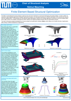


© Copyright 2026