1. science
2. mathematics
3. geometry

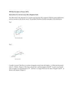
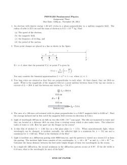
A Supercooled Spin Liquid State
in the Frustrated Pyrochlore Dy2Ti2O7
Ethan R. Kassner1, Azar B. Eyvazov1, Benjamin Pichler1,2, Timothy J. S. Munsie3,4,
Hanna A. Dabkowska3, Graeme M. Luke3,4,5 & J.C. Séamus Davis1,6,7,8
LASSP, Department of Physics, Cornell University, Ithaca, NY 14853, USA
Department of Physics, Stanford University, Palo Alto, CA 94301, USA
3 Brockhouse Institute for Materials Research, McMaster University, Hamilton, ON, Canada.
4 Department of Physics, McMaster University, Hamilton, Ontario, L8S 4M1, Canada.
5 Canadian Institute for Advanced Research, Toronto, Ontario, M5G 1Z8, Canada
6 CMPMS Department, Brookhaven National Laboratory, Upton, NY 11973, USA.
7 School of Physics , University of St. Andrews, St. Andrews, Fife KY16 9SS, Scotland.
8 Kavli Institute at Cornell for Nanoscale Science, Cornell University, Ithaca, NY 14850, USA.
1
2
A ‘supercooled’ liquid develops when a fluid does not crystallize upon cooling below
its ordering temperature. Instead, the microscopic relaxation times diverge so rapidly
that, upon further cooling, equilibration eventually becomes impossible and glass
formation occurs. Classic supercooled liquids exhibit specific identifiers including
microscopic relaxation times diverging on a Vogel-Tammann-Fulcher (VTF)
trajectory, a Havriliak-Negami (HN) form for the dielectric function 𝜺(𝝎, 𝑻), and a
general Kohlrausch-Williams-Watts (KWW) form for time-domain relaxation.
Recently, the pyrochlore Dy2Ti2O7 has become of interest because its frustrated
magnetic interactions may, in theory, lead to highly exotic magnetic fluids. However,
its true magnetic state at low temperatures has proven very difficult to identify
unambiguously. Here we introduce high-precision, boundary-free magnetization
transport techniques based upon toroidal geometries and gain a fundamentally new
understanding of the time- and frequency-dependent magnetization dynamics of
Dy2Ti2O7. We demonstrate a virtually universal HN form for the magnetic
susceptibility 𝝌(𝝎, 𝑻), a general KWW form for the real-time magnetic relaxation, and
a divergence of the microscopic magnetic relaxation rates with precisely the VTF
trajectory. Low temperature Dy2Ti2O7 therefore exhibits the characteristics of a
supercooled magnetic liquid; the consequent implication is that this translationally
invariant lattice of strongly correlated spins is evolving towards an unprecedented
magnetic glass state, perhaps due to many-body localization of spin.
1
Supercooled Liquids
Cooling a pure liquid usually results in crystallization via a first order phase
transition. However, in glass-forming liquids when the cooling is sufficiently rapid, a
metastable ‘supercooled’ state is achieved instead (1-3). Here, the microscopic relaxation
times diverge until equilibration of the system is no longer possible at a given cooling rate.
At this juncture there is generally a broad peak in the specific heat preceding the glass
transition, at which no symmetry breaking phase transition occurs (Fig. 1A). The antecedent
fluid exhibits a set of phenomena characteristic of the supercooled liquid state (1-3). For
example, the divergence of microscopic relaxation times 𝜏0 (𝑇) typically shows substantial
departures from Arrhenius behavior (𝜏0 (𝑇) = 𝐴exp(Δ⁄𝑘𝑇)) and, instead, is described
characteristically using the Vogel-Tammann-Fulcher (VTF) form (4)
𝐷𝑇
𝜏0 (𝑇) = 𝐴exp (𝑇−𝑇0 )
(1)
0
Here 𝑇0 is a temperature at which the relaxation time diverges to ∞ while D characterizes
the extent of the super-Arrhenius behavior (Fig. 1B). One way to establish 𝜏0 (𝑇) is by
measuring the characteristic frequency 𝜔0 (𝑇) = 1/𝜏0 (𝑇) of peaks in the dissipative
(imaginary) component of the dielectric function 𝜀(𝜔, 𝑇). For classic supercooled liquids,
𝜀(𝜔, 𝑇) generally exhibits the Havriliak-Negami (HN ) form (5,6)
𝜀(𝜔, 𝑇) = 𝜀∞ +
𝜀0
(2)
(1+(𝑖𝜔𝜏𝐻𝑁 )𝛼 )𝛾
Here the exponents α and γ describe, respectively, the broadening and asymmetry of the
relaxation in frequency compared to a simple Debye form (=1), 𝜏𝐻𝑁 (𝑇) is the microscopic
relaxation time, and 𝜖∞ is a purely real quantity that describes the relaxation in the 𝜔 → ∞
limit. The HN forms of 𝑅𝑒[𝜀(𝜔, 𝑇)] and 𝐼𝑚[𝜀(𝜔, 𝑇)] that are characteristic of supercooled
liquids are shown in Fig. 1C. In the time domain, this relaxation is described by the classic
Kohlrausch-Williams-Watts (KWW) form (7)
𝜀(𝑡) = 𝜀0 exp [− (𝜏
𝑡
𝐾𝑊𝑊
𝛽
) ]
(3)
where 𝜀(𝑡) describes the evolution of polarization P(t), 𝜏𝐾𝑊𝑊 is the microscopic relaxation
time, and 0< 𝛽 <1 is a “stretching exponent” (Fig. 1D). Debye relaxation corresponds to 𝛽 =
1 while 𝛽 < 1 typically indicates the presence of a more complex energy barrier distribution.
Although the KWW function has no analytic Fourier transform when 𝛽 ≠ 1/2, KWW and HN
2
are actually complementary descriptions of the same microscopic phenomena, being
connected by the relations (8)
ln (𝜏
𝜏𝐻𝑁
𝐾𝑊𝑊
) = 2.6(1 − 𝛽)0.5 exp(−3𝛽) with 𝛼𝛾 = 𝛽1.23 (4)
Observation of this HN / KWW phenomenology is the generally used standard by which
classic supercooled fluids are identified (1,2,3,4).
Magnetization Dynamics Studies of Dy2Ti2O7
Frustrated magnetic pyrochlores are now the focus of widespread interest because of
the possibility that they can support different exotic magnetic phases (9-14). The pyrochlore
Dy2Ti2O7 is one of the most widely studied; it consists of highly-magnetic Dy3+ ions in a sublattice comprised of corner-sharing tetrahedra (Fig. 2A), and an interpenetrating octahedral
lattice of Ti4+ ions playing no magnetic role. Crystal fields break the angular-momentumstate degeneracy and cause the Dy3+ moments (𝐽 =
15
2
, 𝜇 ≈ 10𝜇𝐵 ) to point along their local
[111] directions (15). Although high-temperature susceptibility measurements indicate a
Curie-Weiss temperature of ~1.2K (16), both low temperature susceptibility (16) and muon
spin rotation studies (17) have revealed no magnetic ordering transition in Dy2Ti2O7 down
to T~50 mK. Additionally, a broad peak in the specific heat (18-22) centered around 𝑇 ≈ 1.0
K occurs at or below the transition temperature that might be expected from the Curie-Weiss
temperature, but no phase transition occurs. By contrast, in a typical paramagnet the heat
capacity would exhibit a sharp peak at the ordering temperature below which long-range
magnetic order would become apparent in for example the susceptibility, muon spin
rotation, and neutron scattering; none of these ordering indications are observed in
Dy2Ti2O7. Instead, dipole and exchange interactions combine to create an effective nearestneighbor Ising interaction of the form −𝐽𝑒𝑓𝑓 ∑𝑺𝑖 ⋅ 𝑺𝑗 with 𝐽𝑒𝑓𝑓 ≈ 1.1 K (23). A consequence
of this interaction in the pyrochlore geometry is that there are six possible equivalent
magnetic ground state conformations of a single Dy2Ti2O7 tetrahedron; these can be mapped
to the Bernal-Fowler (“2-in, 2-out”) rules that govern hydrogen bond configurations in water
ice but now it is a 2-in, 2-out arrangement of Dy3+ moments (Fig. 2B). This elegant ‘spin-ice’
configuration has been firmly established (10,14,21,22,24). Theoretically, the long range
3
dipole interactions can also generate magnetic ordering (10,14,25) but, significantly, this has
not been observed down to temperatures below 50mK.
The magnetic excited states of Dy2Ti2O7 are then of great interest. One conjecture is
that the magnetization dynamics may be described as a fluid of emergent delocalized
magnetic monopoles (26). The widely-used dipolar spin-ice model (DSIM) (23) can be used
to derive this magnetic monopoles in spin-ice (MMSI) picture. DSIM incorporates nearestneighbor exchange interactions and long-range dipole interactions:
𝐻𝐷𝑆𝐼 = −𝐽 ∑ 𝑺𝑖 ⋅ 𝑺𝑗 + 𝐷𝑎3 ∑ (
<𝑖𝑗>
𝑖<𝑗
𝑺𝑖 ⋅ 𝑺𝑗
|𝒓𝑖𝑗 |
3
−
3(𝑺𝑖 ⋅ 𝒓𝑖𝑗 )(𝑺𝑗 ⋅ 𝒓𝑖𝑗 )
|𝒓𝑖𝑗 |
5
)
(5)
where a is the nearest-neighbor distance between moments, J is an exchange strength, and
𝐷 = 𝜇0 𝜇 2 /(4𝜋𝑎3 ) is a nearest-neighbor dipole energy scale. This Hamiltonian is
mathematically equivalent to a model where flips of the real Dy3+ dipoles are recast as two
opposite magnetic charges which, though a sequence of spin flips, are hypothesized to form
a fluid of delocalized magnetic monopoles (red and green in Fig. 2C) (26). At low
temperatures these monopoles might then form a dilute neutral gas analogous to an
electrolyte, so that a Debye-Hückel electrolyte model (27) suitably modified for magnetic
monopoles, may be used to describe a ‘magnetolyte’ state (28). Such a mobile fluid of
magnetic monopole excitations, if extant, would constitute a highly novel magnetic state.
However, many observed properties of Dy2Ti2O7 remain unexplained when they are
analyzed using the DSIM/MMSI models. Though DSIM captures some of the diffuse neutron
scattering features of Dy2Ti2O7, simulations based on Eqn. (5) give an incomplete description
of the data; additional exchange contributions from next-nearest and third-nearest
neighbors are required to actually fit the measured scattering intensities precisely (29).
Similarly, while the magnetic susceptibility 𝜒(𝜔, 𝑇) = 𝜒 ′ (𝜔, 𝑇) − 𝑖𝜒 ′′ (𝜔, 𝑇) is known
empirically with high precision (30-33) no accurate quantitative model based on internally
consistent parameterizations of 𝜒 ′ (𝜔, 𝑇) and 𝜒 ′′ (𝜔, 𝑇) has been achieved using DSIM/MMSI
(or any other) models. Moreover, the measured susceptibility of Dy2Ti2O7 cannot be
4
described by the simple Debye form (e.g Eqn. 2 with =1) that would be expected of a
typical paramagnet (33). Microscopic approaches have also failed to capture precisely the
Dy2Ti2O7 magnetization dynamics. For example, DSIM simulations do not accurately
reproduce the measured 𝜒(𝜔, 𝑇) data at low temperatures (34). Furthermore, below ~ 0.5K
macroscopic relaxation rates in Dy2Ti2O7 become ultra-slow (20,21,30,33,35,36,37); this
reflects a divergence of microscopic relaxation times (30,33) that is unexplained
quantitatively within the present DSIM/MMSI models. Thus, although Debye-Hückel
calculations (28) and DSIM/MMSI simulations (38,39) offer clear improvements over a
simple Arrhenius form for 𝜏(𝑇), they still significantly underestimate the observed
magnitude and rate of increase of 𝜏 below 1 K. In fact, as emphasized in a recent review (14),
no studies of Dy2Ti2O7
have yielded direct and unambiguous evidence of a fluid of
delocalized magnetic monopoles. This motivates the search for a more accurate
identification and understanding of the low temperature magnetic state of this important
compound.
Experimental Methods
To explore these issues, we introduce a novel high-precision, boundary-free
technique for studying magnetization transport in Dy2Ti2O7. The innovation consists
primarily of using a toroidal geometry for both the Dy2Ti2O7 samples and the magnetization
sensors, an arrangement with several important benefits. The first is that the
superconducting toroidal solenoid (STS) can be used to both drive magnetization flows
azimuthally and to simultaneously and directly detect dM/dt throughout the whole torus.
More significantly, this topology removes any boundaries in the direction of the
magnetization transport. To achieve this sample topology, holes were pierced through disks
of single-crystal Dy2Ti2O7 (SI Section 1). A superconducting toroidal solenoid of NbTi wire
(diameter~ 0.1 mm) is then wound around each Dy2Ti2O7 torus (SI Section 1). Typical
samples had an ID ~ 2.5 mm, OD ~ 6 mm, and thickness ~ 1 mm. The superconducting
circuitry used to drive and measure dM/dt is shown schematically in Fig. 2D, along with
indicators of the azimuthal B generated by the STS (blue arrows) and the putative flow of a
mixed-sign monopole fluid (red/green arrows).
The all-superconducting 4-point I-V
5
measurement circuit used to generate the B-field and simultaneously measure the EMF
induced by dM/dt is shown schematically in Fig. 2D. These toroidal sample/coil assemblies
were mounted on a dilution refrigerator and studied at temperatures 30mK<T<3K, and
using currents not exceeding 30 mA in the STS (B < ~ 1 G, so always in the low-field limit
𝜇𝐵 ≪ 𝑘𝐵 𝑇).
Time-domain Measurements
Elementary magnetization dynamics experiments in the time-domain are then
carried out using the following repeated measurement cycle. First, a current (and thus B) is
switched on in the STS and the EMF across this same coil V(t) is measured from when the
switch-on transient ends until V(t) drops below our noise level. Next, the current (and B)
is turned off and we again measure the V(t) response. The current is then turned on in the
reverse direction (-B for the same time interval and turned off for the same time interval,
and the procedure is repeated. Complete data sets for this sequence as a function of
temperature are shown in SI Section 3.
Fig. 3A shows the time-dependent magnetization of Dy2Ti2O7 determined from
V(𝑡, 𝑇) ∝ 𝑑𝑴/𝑑𝑡[𝑡, 𝑇] at each temperature (Fig. 3A). To study these measurements in the
context of KWW, we fit each transient 𝑉(𝑡, 𝑇) to the KWW function Eqn. 3 and determine
𝜏𝐾𝑊𝑊 (𝑇) and 𝛽(𝑇). The results are shown directly by plotting the measured log
𝑉(𝑡)
𝑉0
versus
𝑥(𝑡) ≡ ((𝑡)/𝜏𝐾𝑊𝑊 (𝑇))𝛽(𝑇) in Fig. 3B; for these temperatures β ~ 0.75. There we see that, for
all measured transients over a range 575mK < T < 900mK, the 𝑑𝑴/𝑑𝑡 of Dy2Ti2O7 is very
well represented by a KWW time dependence. This puts the ultra-slow magnetization
dynamics in the same empirical class as classic supercooled liquids (1-4). Stretchedexponential relaxation has been previously seen in studies of single-crystal rods of Dy2Ti2O7
(37) but there it was proposed that this relaxation occurred due to the open boundary
conditions. However, our sample topology is a physical realization of periodic boundary
conditions implying that our observed KWW relaxation is actually a fundamental property
of the system. Thus, while simulations of the DSI and delocalized MMSI models in periodic
boundary conditions explicitly rule out stretched-exponential relaxation of magnetization in
Dy2Ti2O7 (39), our measurement results exhibit these characteristics comprehensively.
6
Frequency-domain measurements
If KWW magnetization transient dynamics as in Fig. 3 are evidence for supercooling
of a correlated magnetic fluid, the equivalent phenomena should also be observed as a
universal HN form for the frequency-dependent complex magnetic susceptibility 𝜒(𝜔, 𝑇). To
explore this possibility, we apply sinusoidal currents 𝐼0 Cos(𝜔𝑡) to the STS and generate a
field BCos(𝜔𝑡 + 𝜙) while simultaneously detecting the resulting EMF: 𝑉(𝜔, 𝑇) = 𝑉𝑥 (𝜔, 𝑇) +
𝑖𝑉𝑦 (𝜔, 𝑇). Here the 𝑉(𝜔, 𝑇) is due to temperature dependent changes in the sample
dynamical magnetization (SI Section 2). Directly from the experimental setup (SI Section 2)
one can write
𝑉𝑥 (𝜔, 𝑇) = −𝐼0 𝜔𝐿𝜒 ′′ , 𝑉𝑦 (𝜔, 𝑇) = −𝐼0 𝜔𝐿𝜒′ where L is the effective
geometrical inductance of the STS. A complete set of 𝜒 ′ (𝜔, 𝑇) and 𝜒 ′′ (𝜔, 𝑇) measured in this
fashion is shown in Fig 4A,B and described in SI Section 2. Equivalent phenomena were
measured in three different Dy2Ti2O7 tori ruling out any specific sample preparation or
torus/coil geometry effects as the cause of reported phenomena. Empirically, the
temperature and frequency dependence of the 𝜒 ′ (𝜔, 𝑇) and 𝜒 ′′ (𝜔, 𝑇) in our studies is
virtually identical to what has been reported previously. Until now, however, no quantitative
internally consistent model for the susceptibility of Dy2Ti2O7 has been identified. Here, we
show that a HN form for a magnetic susceptibility
𝜒
𝜒𝐻𝑁 (𝜔, 𝑇) = 𝜒∞ + (1+(𝑖𝜔𝜏0
𝐻𝑁 )
𝛼 )𝛾
(6)
provides a comprehensive accurate internally consistent description for both 𝜒 ′ (𝜔, 𝑇) and
𝜒 ′′ (𝜔, 𝑇) of Dy2Ti2O7. To achieve this, we need to demonstrate that all our disparate 𝜒(𝜔, 𝑇)
data has the same HN functional form. We define a scaled susceptibility 𝐺(𝛾, 𝜒) that depends
only upon  𝜒0 and 𝜒(𝜔, 𝑇):
Re[𝐺(𝛾, 𝜒)] ≡
Im[𝐺(𝛾, 𝜒)] ≡
−1/𝛾
𝜒0 [(𝜒 ′ )2
−1/𝛾
𝜒0 [(𝜒 ′ )2
+
+
1
(𝜒 ′′ )2 ]2𝛾
1
(𝜒 ′′ )2 ]2𝛾
1
𝜒 ′′
cos [ arctan ( ′ )]
𝛾
𝜒
(7)
1
𝜒 ′′
sin [ arctan ( ′ )]
𝛾
𝜒
where we have neglected 𝜒∞ because it is much smaller than 𝜒0 at our experimental
temperatures (SI Section 2). As shown analytically in SI Section 2, if plotting
Re[𝐺(𝛾, 𝜒)] and Im[𝐺(𝛾, 𝜒)] vs. (𝜔𝜏)𝛼 collapses 𝜒(𝜔, 𝑇) data onto a single curve, then the
7
magnetic susceptibility exhibits a universal HN form. Figure 4C,D show this data collapse for
all measured 𝜒(𝜔, 𝑇) where the fine solid line is the model HN form of Eqn. 6. It is clear that
𝜒𝐻𝑁 (𝜔, 𝑇) fits the observed Dy2Ti2O7 data precisely and comprehensively. To our knowledge,
this is the first time that both 𝜒 ′ (𝜔, 𝑇) and 𝜒 ′′ (𝜔, 𝑇) of Dy2Ti2O7 have been quantitatively
and simultaneously described by a single internally-consistent function, across very wide
frequency/temperature ranges and with Kramers-Kronig consistency. More importantly,
since this HN form for magnetic susceptibility is functionally indistinguishable from the
𝜀(𝜔, 𝑇) of supercooled liquids (1-3) it strongly implies supercooling of a correlated magnetic
fluid in this compound.
Diverging Microscopic Relaxation Rates
A final test of the supercooled magnetic liquid hypothesis would be to show that the
magnetic relaxation times diverge on a VTF trajectory for Dy2Ti2O7. To determine
microscopic relaxation times 𝜏0 (T) spanning the whole temperature range, we use 𝜏𝐻𝑁 (T)
from fitting Eqn. 6 simultaneously to 𝜒 ′ (𝜔, 𝑇) and 𝜒 ′′ (𝜔, 𝑇) for 0.8K < T < 3K, and 𝜏𝐾𝑊𝑊 (T)
from the time-domain V(t,T) fitted by Eqn. 3 and then converted to the equivalent 𝜏𝐻𝑁 (T)
for 0.58K<T<0.85K using Eqn. 4. As shown in Fig. 4E the resulting 𝜏𝐻𝑁 (T) of Dy2Ti2O7 can,
indeed, be represented by a VTF function (Eqn. 1) with high precision over many orders of
magnitude (𝑇0 ≈ 0.24K and fragility parameter 𝐷 ≈ 14). This unifies the evidence (Figs. 3,4)
that the magnetic state of Dy2Ti2O7 for 0.5 K < T < 3K is a supercooled magnetic liquid.
Conclusions and Discussion
One may now reconsider the anomalous phenomena of Dy2Ti2O7 in this new context.
Empirically, our measured 𝜒(𝜔, 𝑇) data are in good agreement with earlier reports (30-33)
implying that all can be describable by a HN susceptibility (Eqn. 2; Fig. 4A,B). Also, while the
Curie-Weiss temperature TCW~1.2K (16) implies a tendency towards ferromagnetic order,
no ordering is observed and, instead, a broad peak in specific heat C(T) appears just below
TCW (18,19,20,21,22); this is as expected for a supercooled liquid (Fig. 1A and Refs. 1-3). The
location of Dy3+ moments in the highly anisotropic environment of the Dy2Ti2O7 prevents
ferromagnetic ordering at a temperature that might be expected from the nearest-neighbor
interaction energy scale; this may be analogous to preventing the onset of a crystalline phase
8
in glass-forming liquids due to anisotropic interactions between molecules. Moreover, ultraslow macroscopic equilibration is widely reported at lower temperatures (20, 35,37) and is
also is just what one expects in a supercooled liquid approaching the glass transition (1-3).
Our observed stretched-exponential form for ultra-slow magnetization relaxation agrees
well with previous studies (37). While actually at odds with the predictions of DSIM/MMSI
simulations for periodic geometries (39) this phenomenon is characteristic of a supercooled
fluid (1,2,3). Finally, the published data on divergences of microscopic relaxation times
(30,33) are in good empirical agreement with ours, implying that the VTF form for(T) is
general for Dy2Ti2O7 (Eqn. 1, Fig 4E). Thus we conjecture that overall magnetization
dynamics of Dy2Ti2O7 are best explained if the system is a classical correlated-spin liquid that
that is supercooled and approaching a glass transition. Within this picture, the divergence
temperature 𝑇0 ≈ 240 mK derived from our VTF fit (Fig. 4E) provides an estimate of the
lowest temperature at which a metastable magnetic liquid state can survive under arbitrary
cooling protocols; below this temperature we expect that Dy2Ti2O7 must transition into
either a heterogeneous glass phase or a phase with global magnetic order.
To recapitulate: for the magnetic pyrochlore system Dy2Ti2O7 we discover that the
magnetic susceptibility 𝜒(𝜔, 𝑇) exhibits a Havriliak-Negami form, the magnetic relaxation
𝜒(𝑡) simultaneously exhibits the Kohlrausch-Williams-Watts form, while the microscopic
magnetic relaxation rates 𝜏(T) occur on the Vogel-Tammann-Fulcher trajectory. When, in
combination with a broad specific heat peak, this phenomenology is observed for the 𝜀(𝜔, 𝑇)
of a classic glass forming material, it definitely identifies a supercooled liquid (1-3). Our
observations therefore strongly imply that the magnetic state of Dy2Ti2O7 is a supercooled
classical spin liquid, approaching a glass transition. However, we emphasize that one should
not expect any consequent magnetic glass to be a classic spin glass, because all the Dy2Ti2O7
spins are at ordered crystal lattice sites with locally identical spin Hamiltonians. And, indeed,
Dy2Ti2O7 is known to exhibit a very different field-dependence from what is seen in classical
spin glasses (30). The supercooled liquid characteristics of magnetization dynamics in
Dy2Ti2O7 (Fig.s 3,4) more likely imply some form of persistent heterogeneous freezing in the
microscopic configurations of strongly correlated spins (40,41). Such a situation could also
9
be described (somewhat redundantly) as freezing of monopole configurations. However, in
terms of actual magnetization transport, the observed stretched-exponential time
dependence of magnetization (Fig. 3, Ref. 37) contradicts the predicted dynamics of both
DSIM and MMSI models (39). Instead, one intriguing possibility is that the state of Dy2Ti2O7
actually represents translationally-invariant many-body localization of the spins (42,43,44).
It will be fascinating, in this context, to reconsider the absence of magnetic ordering in other
frustrated pyrochlores so as to determine if supercooled classical spin liquids occur therein.
Acknowledgements: We are grateful to E. Fradkin, B. Gaulin, M. Gingras, S. Grigera, D.
Hawthorn, R. Hill, E.-A. Kim, J. Kycia, M.J. Lawler, A.P. Mackenzie, R. Melko, and J. Sethna for
very helpful discussions and communications. This research is funded by the Gordon and
Betty Moore Foundation’s EPiQS Initiative through Grant GBMF4544 and by the EPSRC
Programme Grant ‘Topological Protection and NonEquilibrium States in Correlated
Electron Systems’.
10
FIGURE CAPTIONS
Figure 1: Signatures of Supercooling in Classic Glass-forming Fluids
A. Under suitable conditions, a liquid can be cooled through the melting temperature 𝑇𝑚
without crystallizing and instead reaches a supercooled liquid state. With further cooling,
the heat capacity of the supercooled liquid must eventually decrease from the higher
liquid value toward the lower crystalline value; this is necessary for the entropy to
remain non-negative at very low temperatures. Supercooled liquids therefore typically
have a broad peak in their heat capacity below 𝑇𝑚 and a little above the glass transition
temperature 𝑇𝑔 .
B. In a classic supercooled liquid, diverging microscopic relaxation times 𝜏0 (𝑇) typically do
not follow Arrhenius behavior (dashed line) but instead follow the Vogel-TammannFulcher (VTF) evolution (blue curve; Eqn. 1). Here 𝑇0 is a temperature at which the
relaxation time diverges to ∞ while D characterizes the extent of the super-Arrhenius
behavior. By convention, a classic glass is said to form when𝜏0 >100s.
C. 𝑅𝑒[𝜀(𝜔, 𝑇)] and 𝐼𝑚[𝜀(𝜔, 𝑇)] of the Havriliak-Negami form (Eqn. 2) of the dielectric
function; these are both characteristic of supercooled liquids.
D. Ultra-slow relaxation in glass-forming liquids occurs with a KWW form (green curve,
Eqn. 3) instead of a Debye form (dashed line), as shown here for the dielectric function
(t).
Figure 2: Novel Experimental Techniques for Frustrated Magnetism in Dy2Ti2O7
A. The Dy3+ moments (black circles) in Dy2Ti2O7 are located on a lattice comprised of
equilateral corner-sharing tetrahedra. The centers of tetrahedra themselves form a
diamond lattice.
B. An allowed magnetic ground-state configuration for two tetrahedra in Dy2T2iO7. Here the
crystal field anisotropy causes the moments to point along their local [111] axes, thus
forcing them to point toward or away from each tetrahedron center. To minimize
11
magnetic energy, the spin configurations of a tetrahedron of Dy2T2iO7 satisfy the spin
equivalent of the Bernal-Fowler ‘ice rules’, with each tetrahedron having two spins
pointing toward its center and two spins pointing away from its center.
C. Schematic of a pair of delocalized magnetic monopoles (+ green, - red) representing a
sequence of spin flips as shown.
D. Schematic representation of the toroidal geometry of our Dy2Ti2O7 sample (yellow) and
the superconducting toroidal solenoid (blue). The cryogenic sample environment
30mK<T<4K is indicated by a dashed rectangle. DC current flow in the direction indicated
by black arrow produces an azimuthal static magnetic field B(blue arrows). If a fluid of
magnetic-monopoles of both signs exists, the net magnetization current J (red/green
arrows) would be nonzero. Applied AC currents 𝐼0 𝐶𝑜𝑠(𝜔𝑡) generate the azimuthal fields
H𝐶𝑜𝑠(𝜔𝑡) whose effect is simultaneously detected by measuring the EMF across the
STS: 𝑉(𝜔, 𝑇). The dynamical magnetic susceptibility components are then derived from
𝑉𝑥 (𝜔, 𝑇) = −𝐼0 𝜔𝐿𝜒 ′′ , 𝑉𝑦 (𝜔, 𝑇) = −𝐼0 𝜔𝐿𝜒′, where L is the effective geometrical
inductance of the STS.
Figure 3: Kohlrausch-Williams-Watts Magnetization Transient Dynamics
A. Typical examples of measured V(t,T) of Dy2Ti2O7 torus after the current is switched off in
the STS.
B. The KWW collapse of all measured V(t,T) transients from our Dy2Ti2O7 torus experiments
at the temperatures shown. Clearly, a KWW relaxation model provides an excellent
description of the data over the entire range of temperatures at which we could resolve
the dM/dt signals.
12
Figure 4: Havriliak-Negami Magnetic Susceptibility and Vogel-Tammann-Fulcher
Microscopic Relaxation Times
A. Measured frequency and temperature dependence of the real component of the magnetic
susceptibility calculated from the EMF component 𝑉𝑦 that is 90-degrees out of phase with
the applied field.
B. Measured frequency and temperature dependence of the imaginary component of the
magnetic susceptibility calculated from the EMF component 𝑉𝑥 that is in phase with the
applied field.
C. To demonstrate that the Dy2Ti2O7 magnetic susceptibility 𝜒(𝜔, 𝑇) is comprehensively
described by a Havriliak-Negami form, we define in Eqn. 7 a scaled susceptibility 𝐺(𝛾, 𝜒)
depending only upon  𝜒0 and 𝜒(𝜔, 𝑇) . Here we plot Re[𝐺(𝛾, 𝜒)] vs. (𝜔𝜏)𝛼 for all our
measured 𝜒(𝜔, 𝑇) showing a very high precision collapse of all our data to the HN form
(shown as a solid line for [𝜒0 = 1, 𝛾 = 1, 𝜏𝐻𝑁 = 1, 𝛼 = 0.91]). The fit values of γ(T) and
α(T) are shown in the insets.
D. Im[𝐺(𝛾, 𝜒)] plotted versus vs. (𝜔𝜏)𝛼 for all measured 𝜒(𝜔, 𝑇) again showing a high
precision collapse of all our data to the HN form (shown as a solid line for [𝜒0 = 1, 𝛾 =
1, 𝜏𝐻𝑁 = 1, 𝛼 = 0.91]) with identical parameters as in A. The fit values of 𝜒0 are shown
in the inset.
E. Measured microscopic relaxation times 𝜏𝐻𝑁 (T) for magnetization in Dy2Ti2O7 spanning
the whole temperature range 0.575 K< T < 3 K plotted versus (T-To)-1 where To = 242 mK.
This demonstrates clearly that magnetic relaxation in Dy2Ti2O7 is governed by the VTF
form (Eqn. 1) over almost four orders of magnitude in 𝜏𝐻𝑁 .
13
FIGURE 1
14
FIGURE 2
A
B
C
D
15
FIGURE 3
A
B
16
FIGURE 4
B
A
C
D
E
17
REFERENCES
1
Ediger M, Angell C, Nagel S (1996) Supercooled Liquids and Glasses. J. Phys. Chem.
100:13200-13212.
2
Tarjus G, Kivelson S, Nussinov Z, Viot P (2005) The frustration-based approach of
supercooled liquids and the glass transition: a review and critical assessment. J. Phys:
Condens. Matt. 17:R1143-R1182.
3
Cavagna A (2009) Supercooled liquids for pedestrians. Physics Reports 476:51-124.
4
Bohmer R, Ngai K, Angell C, Plazek D (1993) Nonexponential relaxations in strong and fragile
glass formers. J. Chem. Phys. 99:4201-4209.
5
Havriliak S, Negami S (1967) A Complex Plane Representation of Dielectric and Mechanical
Relaxation Processes in Some Polymers. Polymer 8:161-210.
6
Havriliak Jr. S, Havriliak S (1994) Results from an unbiased analysis of nearly 1000 sets of
relaxation data. J. Non-Cryst. Solids 172-174:297-310.
7
Kohlrausch R (1854) Theorie des elektrischen ruckstandes in der leidner flasche. Annelen
der Physik und Chemie (Poggendorff) 91:179-213.
8
Alvarez F, Alegría A, Colmenero J (1991) Relation between the time-domain KohlrauschWilliams-Watts and frequency-domain Havriliak-Negami relaxation functions. Phys. Rev. B
44:7306-7312.
9
Harris M., Bramwell S, Holdsworth P, Champion J (1998) Liquid-Gas Critical Behavior in a
Frustrated Pyrochlore Ferromagnet. Phys. Rev. Lett. 81:4496-4499.
10
(2011) Introduction to Frustrated Magnetism: Materials, Experiments, Theory, eds Lacroix C,
Mendels P, Mila F (Springer Series in Solid-State Sciences, 2011).
11
Gardner J, Gingras M, Greedan E (2010) Magnetic pyrochlore oxides. Rev. Mod. Phys. 82:53107.
12
Balents L (2010) Spin liquids in frustrated magnets. Nature 464:199-208.
13
Castelnovo C, Moessner R, Sondhi S (2012) Spin Ice, Fractionalization, and Topological
Order. Annu. Rev. Condens. Matter Phys. 3:35-55.
14
Gingras M, McClarty P (2014) Quantum spin ice: a search for gapless quantum spin liquids
in pyrochlore magnets. Rep. Prog. Phys. 77:056501.
18
15
Rosenkranz S et al (2000) Crystal-field interaction in the pyrochlore magnet Ho2Ti2O7.
Journal of Applied Physics 87:5914-5916.
16
Fukazawa H, Melko R, Higashinaka R, Maeno Y, Gingras M (2002) Magnetic anisotropy of the
spin-ice compound Dy2Ti2O7. Phys. Rev. B 65:054410.
17
Dunsiger S et al. (2011) Magnetic Excitations without Monopole Signatures using Muon Spin
Rotation. Phys. Rev. Lett. 107:207207.
18
Klemke B et al. (2011) Thermal Relaxation and Heat Transport in the Spin Ice Material
Dy2Ti2O7. J. Low Temp. Phys. 163:345-369.
19
Higashinaka R, Fukazawa H, Yanagishima D, Maeno Y (2002) Specific heat of Dy2Ti2O7 in
magnetic fields: comparison between single-crytalline and polycrystalline data. J. Phys.
Chem. Solids. 63:1043-1046.
20
Pomaranski D et al. (2013) Absence of Pauling’s residual entropy in thermally equilibrated
Dy2Ti2O7. Nat. Phys. 9:353–356.
21
Ramirez A, Hayashi A, Cava R, Siddharthan R (1999) Zero-point entropy in ‘spin ice’. Nature
399:333-335.
22
Morris D et al. (2009) Dirac Strings and Magnetic Monopoles in the Spin Ice Dy2Ti2O7.
Science 326:411-414.
23
den Hertog B, Gingras M (2000) Dipolar Interactions and the Origin of Spin Ice in Ising
Pyrochlore Magnets. Phys. Rev. Lett. 84:3430.
24
Bramwell S, Gingras M (2001) Spin Ice State in Frustrated Magnetic Pyrochlore Materials.
Science 294:1495-1501.
25
Melko R, Gingras M (2004) Monte Carlo studies of the dipolar spin ice model. J. Phys.
Condens. Matter. 16:R1277–R1319.
26
Castelnovo C, Moessner R, Sondhi S (2008) Magnetic monopoles in spin ice. Nature. 451:4245.
27
Levin Y (2002) Electrostatic correlations: from plasma to biology. Rep. Prog. Phys 65:15771632.
28
Castelnovo C, Moessner R, Sondhi S (2011) Debye-Hückel theory for spin ice at low
temperature. Phys. Rev. B 84:144435.
29
Yavors’kii T, Fennell T, Gingras M, Bramwell S (2008) Dy2Ti2O7 Spin Ice: A Test Case for
Emergent Clusters in a Frustrated Magnet. Phys. Rev. Lett. 101:037204.
19
30
Snyder J et al. (2004) Low-temperature spin freezing in the Dy2Ti2O7 spin ice. Phys. Rev. B
69:064414.
31
Matsuhira K et al. (2011) Spin Dynamics at Very Low Temperature in Spin Ice Dy2Ti2O7. J.
Phys. Soc. Japan 80:123711.
32
Bovo L, Bloxsom J, Prabhakaran D, Aeppli G, Bramwell S (2013) Brownian motion and
quantum dynamics of magnetic monopoles in spin ice. Nat. Comm. 4:1535-1542.
33
Yaraskavitch L et al. (2012) Spin dynamics in the frozen state of the dipolar spin ice
Dy2Ti2O7. Phys. Rev. B 85:020410.
34
Takatsu H et al. (2013) AC Susceptibility of the Dipolar Spin Ice Dy2Ti2O7: Experiments and
Monte Carlo Simulations. J. Phys. Soc. Japan 82:104710.
35
Giblin S, Bramwell S, Holdsworth P, Prabhakaran D, Terry I (2011) Creation and
measurement of long-lived magnetic monopole currents in spin ice. Nat. Phys., 7:252-258.
36
Orendáĉ M et al. (2007) Magnetocaloric study of spin relaxation in dipolar spin ice
Dy2Ti2O7. Phys. Rev. B 75:104425.
37
Revell H et al. (2012) Evidence of impurity and boundary effects on magnetic monopole
dynamics in spin ice. Nat. Phys 9:34-37.
38
Jaubert L, Holdsworth P (2009) Signature of magnetic monopole and Dirac string dynamics
in spin ice. Nat. Phys 5:258-261.
39
Jaubert L, Holdsworth P (2011) Magnetic monopole dynamics in spin ice. J. Phys.: Condens.
Matt. 23:164222.
40
Cépas O, Canals B (2012) Heterogeneous freezing in a geometrically frustrated spin model
without disorder: Spontaneous generation of two timescales. Phys. Rev. B 86:024434.
41
Z. Nussinov, C. D. Batista, B. Normand, and S. A. Trugman (2007) High-dimensional
fractionalization and spinon deconfinement in pyrochlore antiferromagnets Phys. Rev. B
75: 094411
42
De Roeck W, F. Huveneers (2014) Scenario for delocalization in translation-invariant
systems. Phys. Rev. B 90:165137.
43
Yao N, Laumann C, Cirac J, Lukin M, Moore J (2014) Quasi Many-body Localization in
Translation-Invariant Systems. arXiv 1410.7407
44
Schiulaz M, Silva A, Müller M, (2014) Dynamics in many-body localized quantum systems
without disorder. arXiv 1410.4690.
20
Supplementary Information for
A Supercooled Spin Liquid State
in the Frustrated Pyrochlore Dy2Ti2O7
Ethan R. Kassner, Azar B. Eyvazov, Benjamin Pichler, Timothy J. S. Munsie,
Hanna A. Dabkowska, Graeme M. Luke & J.C. Séamus Davis
S1. Toroidal Dy2Ti2O7 sample and Toroidal Superconducting Sensor Coil
The Dy2Ti2O7 samples used in this project were synthesized by the Graeme Luke
Group at McMaster University using an optical floating zone furnace. The original sample
boule was grown at a rate of ~ 7mm/hr in O2 gas under 2 atm of pressure, and was
subsequently cut into disks of diameter ~ 6 mm and thickness ~ 1 mm. X-ray diffraction on
the resultant crystal was sharp and showed no signs of twinning or the presence of
multiple grains. Performance of Rietveld refinement on the diffraction data yields a unit cell
lattice constant of 10.129 Å; this implies a maximum possible level of “spin stuffing”
(substitution of Dy3+ ions on Ti4+ sites) of ≈ 2.9% and a most likely spin stuffing fraction <
1%.
To create boundary-free conditions for our measurements of magnetization
dynamics, we pierced holes of diameter ~ 2.5 mm through each Dy2Ti2O7 disk using
diamond-tipped drill bits. Fig. S1A shows two typical samples after the completion of the
drilling process. We also manufactured equivalent tori from Stycast 1266 for control
measurements; these were cut and drilled to match the geometrical details of our Dy2Ti2O7
samples. Because Stycast 1266 has negligible magnetic activity in our parameter space, it
functioned as a good material for control tests; we observed no significant temperaturedependent magnetic signals in this epoxy.
CuNi-clad NbTi wire (thickness 0.1 mm) was wound around each toroidal Dy2Ti2O7
sample creating a superconducting toroidal solenoid (STS) (Fig S1B). Lakeshore varnish
(VGE-7031) was used to mount our samples on a stage connected to the mixing chamber of
a dilution refrigerator and performed measurements at temperatures from 30 mK up to 3
1
K. Sample temperature was measured with a Lakeshore RuO2 (RoxTM) thermometer, and
temperature was controlled using a Lakeshore 370 AC Resistance Bridge.
S2. AC magnetization dynamics experiments
For AC measurements four-probe I-V circuit configuration (Fig 2D in the main text)
was utilized . A lock-in amplifier was used to apply AC currents (of up to 30 mA) to the STS
and to simultaneously measure the STS EMF. We begin our AC analysis by writing the STS
EMF in terms of the changing magnetic flux:
𝑉=−
𝑑Φ
𝑑𝐵
𝑑
= −𝑁𝐴
= −𝑁𝐴𝜇0 (𝐻 + 𝑀)
𝑑𝑡
𝑑𝑡
𝑑𝑡
where N is the number of coil turns in the STS and A is the effective coil cross-sectional
area. Using the standard definition of the frequency-dependent magnetic volume
susceptibility, 𝑀(𝜔) = 𝜒(𝜔)𝐻(𝜔), and the applied magnetic field 𝐻 = 𝑛𝐼exp(𝑖𝜔𝑡), one can
calculate the amplitude of the STS EMF:
𝑉(𝜔) = −𝜇0 𝑁𝐴𝑛𝐼𝑖𝜔(1 + 𝜒(𝜔)) = −𝑖𝐼𝜔𝐿(1 + 𝜒(𝜔))
(S1)
where N is total number of STS turns, n is the turns/length in the STS, A is the effective
cross-sectional area of the coil, I is the applied current, and L is the effective geometric
inductance of the STS. We specifically measured the EMF components that were in phase
(“X”) and 90 degrees out of phase (“Y”) with the applied current: 𝑉 = 𝑉𝑥 + 𝑖𝑉𝑦 . Experiments
on our nonmagnetic Stycast 1266 control sample, which used the same circuitry as our
Dy2Ti2O7 measurements, showed no temperature dependence; all signals in the Stycast
coils were due simply to standard circuit responses to a changing magnetic field. These
observations confirmed that the circuit geometry and conductance in the area of the
experiment had no significant variation in our measured temperature range. Any
temperature-dependent changes in the frequency-dependent STS EMF are due to changes
in the magnetization dynamics of the Dy2Ti2O7 samples.
2
Since the microscopic relaxation times of Dy2Ti2O7 are sensitive to its temperature (1), it
was essential to verify that our samples and measurements stabilized at each set
temperature. We determined thermalization times by performing tests in which we took
lock-in amplifier readings for several hours after temperature and frequency changes;
Figure S2 shows typical results of these measurements. After frequency changes the EMF
readings settled almost immediately (within seconds) to stable long-time values, while the
readings reached stable values after less than 10 minutes following temperature changes.
To accommodate this thermalization time, we waited at least 15 minutes after temperature
changes before recording data in both the AC and DC experiments.
We measured the geometric inductance L of our STS systems by measuring 𝑉𝑦 at
frequencies in the range 40-80 kHz at T=30 mK; these frequencies are well above the
frequency range in which we observed significant Dy2Ti2O7 dynamics, so for these
measurements the STS EMF is dominated by the vacuum inductor signal 𝑉𝑦 = 𝐼𝜔𝐿. From
the linear frequency dependence of 𝑉𝑦 we have found that our typical STS inductances are
1-2 µH.
Figs S3A and S3B show the real and imaginary parts, respectively, of typical STS
EMF data at 500 mK and 900 mK, with 50-mK data treated as background and subtracted.
There is a clear difference in the EMFs measured at 900 mK and 50 mK; we use this
temperature dependence of the STS signals to study the frequency-dependent
magnetization dynamics of Dy2Ti2O7 (see below). At 500 mK, however, the STS EMF is
indistinguishable from the EMF at 50 mK. Previous susceptibility measurements (2)
indicate that Dy2Ti2O7 has negligible magnetic activity in our frequency range (2-1000 Hz)
at temperatures as low as several hundred mK; we therefore assume that the data at 50 mK
is due completely to non-Dy2Ti2O7 sources, and we conclude that all data in our parameter
space taken at T ≤ 500 mK are due to non- Dy2Ti2O7 background sources.
3
For experiments at higher temperatures, we subtracted the 500-mK data to isolate
Dy2Ti2O7 contributions to the STS EMF:
Δ𝑉(𝜔, 𝑇) = 𝑉(𝜔, 𝑇) − 𝑉(𝜔, 500 𝑚𝐾) = Δ𝑉𝑥 (𝜔, 𝑇) + 𝑖Δ𝑉𝑦 (𝜔, 𝑇)
= −𝑖𝐼𝜔𝐿(𝜒 ′ − 𝑖𝜒 ′′ )
where we have used the conventional notation for the complex magnetic volume
susceptibility 𝜒 = 𝜒 ′ − 𝑖𝜒′′. Therefore, the quadrature EMF components can be written as
Δ𝑉𝑥 = −𝐼𝜔𝐿𝜒 ′ ′
(S2)
Δ𝑉𝑦 = −𝐼𝜔𝐿𝜒′
The HN form for a magnetic susceptibility is given by
𝜒(𝜔, 𝑇) = 𝜒∞ +
𝜒0
[1 + (𝑖𝜔𝜏𝐻𝑁 )𝛼 ]𝛾
(S3)
where 𝜒0 is a relaxation amplitude, 𝜏𝐻𝑁 is a characteristic relaxation time, and the
exponents α and γ describe the spread and asymmetry, respectively, of the relaxation in
frequency space. 𝜒∞ gives the relaxation in the 𝜔 → ∞ limit. This model is a generalization
of the simplest complex relaxation models: Debye relaxation has 𝛼 = 1, 𝛾 = 1; Cole-Cole
relaxation has 𝛾 = 1; and Davidson-Cole relaxation has 𝛼 = 1. Figures S4A and S4B show
the quadrature susceptibility components at two representative temperatures, along with
fits to Debye and HN forms. Debye relaxation is clearly an inadequate description of our
data; one needs the full set of HN parameters to reproduce the observed magnetization
dynamics.
Figures S5A and S5B show the full set of real and imaginary parts of the
susceptibility using and Equation (S2). These experiments were performed between 0.8 K
and 3 K. We performed simultaneous fits of 𝜒′(𝜔) and 𝜒′′(𝜔) to the HN function using a
least squares method that minimized the cumulative residuals of the real and imaginary
susceptibility components. The solid lines in Figs S5A and B show the results of these fits;
our observations are clearly described very well by HN relaxation. The small residuals
(𝜒′(𝜔, 𝑇) − 𝜒 ′ 𝐻𝑁 (𝜔, 𝑇), inset of Fig. S5A; 𝜒 ′′ (𝜔, 𝑇) − 𝜒 ′′ 𝐻𝑁 (𝜔, 𝑇), inset of Fig. S5B) further
illustrate the quality of these fits; throughout all of our parameter space the residuals are a
4
few percent or less of the signal size. HN spectra are generally found in supercooled liquids.
The temperature dependencies of the HN parameters 𝜒0 (Fig. S6A), 𝜒∞ (Fig. S6B), α (Fig.
S6C), and γ (Fig. S6D) are shown in Fig. S6; 𝜏𝐻𝑁 is shown along with the relaxation times
obtained from our DC experiments in Figure 4E of the main text.
We can further show the broad applicability of HN relaxation to Dy2Ti2O7 dynamics by
finding scaled HN variables that collapse the T-dependent 𝜒′ and 𝜒′′ data onto single
curves. To do this, we start with the basic HN form and separate the exponents α and γ:
𝜒(𝜔, 𝑇) = 𝜒 ′ − 𝑖𝜒′′ =
1/𝛾
𝜒 ′ − 𝑖𝜒′′
(
)
𝜒0
=
𝜒0
[1 + (𝑖𝜔𝜏𝐻𝑁 )𝛼 ]𝛾
1
1 + (𝑖𝜔𝜏𝐻𝑁 )𝛼
(S4)
where we ignore the effects of 𝜒∞ since it is much smaller than 𝜒0 (Figure S6). Using
complex algebra identities, we can write the LHS of Equation (S4) as
1/2𝛾
𝜒′2 + 𝜒′′2
𝐺(𝛾, 𝜒0 , 𝜒) ≡ (
)
𝜒0 2
1
𝜒′′
1
𝜒′′
(cos ( arctan ′ ) − 𝑖 sin ( arctan ′ ))
𝛾
𝜒
𝛾
𝜒
(S5)
and we can write the RHS as
𝜋𝛼
𝜋𝛼
1 + (𝜔𝜏𝐻𝑁 )𝛼 (cos 2 − 𝑖sin 2 )
𝐻(𝛼, 𝜔𝜏𝐻𝑁 ) ≡
𝜋𝛼
1 + 2(𝜔𝜏𝐻𝑁 )𝛼 cos 2 + (𝜔𝜏𝐻𝑁 )2𝛼
(S6)
The real and imaginary components of G give us effective scaled variables for the real and
imaginary susceptibility components, respectively:
Re[𝐺(𝛾, 𝜒0 , 𝜒)] =
−1/𝛾
𝜒0 [(𝜒 ′ )2
−1/𝛾
Im[𝐺(𝛾, 𝜒0 , 𝜒)] = 𝜒0
1
1
𝜒 ′′
′′ )2 ]2𝛾
(𝜒
+
cos [ arctan ( ′ )]
𝛾
𝜒
1
1
𝜒 ′′
[(𝜒 ′ )2 + (𝜒 ′′ )2 ]2𝛾 sin [ arctan ( ′ )]
𝛾
𝜒
5
To complete the data collapse procedure, we need to choose a suitable scaled frequency;
the best choice is 𝑥 ≡ (𝜔𝜏𝐻𝑁 )𝛼 . Using this definition we can rewrite the HN relaxation as
𝜋𝛼
𝜋𝛼
1 + 𝑥(cos 2 − 𝑖sin 2 )
𝐺(𝛾, 𝜒0 , 𝜒) =
𝜋𝛼
1 + 2𝑥cos 2 + 𝑥 2
(S7)
α varies weakly with temperature (Fig. S6C), so with these definitions we achieve excellent
universal collapse of our AC data (Figs. 4C and 4D in the main text). The characteristic
curve of this collapse is a Cole-Cole curve with 𝛼 = 0.91.
S3. Time-domain experiments
During time domain experiments we used a 4-probe superconducting I-V circuit
configuration to apply current to and measure the EMF across our STSs (Fig. 2D in the main
text). For these studies we applied DC currents as high as 25 mA using an Agilent 33210A
Arbitrary Waveform Generator to create a current supply; we simultaneously measured
the STS EMF, V(t), with a Keithley 2182A Nanovoltmeter. As shown in Fig. S7A, the current
application protocol is as follows (green dashed lines): (1) apply current in one direction
for a time interval t, (2) turn off the current for an identical interval t, (3) apply current in
the opposite direction for t, (4) turn off the current for t and then return to step 1. We
typically repeated this sequence hundreds of times to improve our signal-to-noise ratio and
achieve robust fits to the data. Fig S7A depicts a typical complete measurement sequence at
three experimental temperatures. The STS V(t) was measured every 20 milliseconds
throughout the experiment, and we observed that 20 seconds is sufficient for the induced
EMF to drop below our noise level ~1 nV at all temperatures above 550 mK. Our ability to
resolve decay curves at higher temperatures was limited by the time resolution of the
nanovoltmeter.
Our V(t) are direct measurements of changes in the sample magnetization density M
over time:
6
𝑑Φ
𝑑(𝑀 + 𝐻)
= −𝜇0 𝑁𝐴
𝑑𝑡
𝑑𝑡
𝑑𝑀
𝑑𝐻
= −𝜇0 𝑁𝐴
− 𝜇0 𝑁𝐴
𝑑𝑡
𝑑𝑡
𝑉 = −𝑁
(S8)
where N is the number of coil turns in the STS and A is the effective STS cross-sectional
area. The second term, which describes the STS response to changes in the applied field
itself, is present even when the STS encloses vacuum. Since the only change in H occurs
when we turn the applied current on or off, the contributions of this term are limited to
very short times (< ~ 100 ms) after current changes. For our fits we examined data taken ≥
200 ms after current changes, when only the first term in Equation (S8) contributes.
We can relate the measured EMF to the time-dependent magnetic volume
susceptibility χ(t) by considering the STS as having inductance L with I as the fieldgenerating current. Taking the time derivative of M(t) and inserting it into Equation (S8)
gives the final expression for the long-time STS EMF:
𝑉 = 𝐼𝐿𝜒(𝑡)
(S9)
Fig S7B depicts the typical measured EMF (symbols) generated for t ≥ 200 ms after
turning off the STS current at temperatures from 575 mK up to 900 mK; at these times the
EMF is given by Equation (S9). The STS EMF shows slower-than-exponential decay, and the
decay times increase dramatically with decreasing temperature. The lines in Fig. S6B are
fits to the Kohlrausch-Williams-Watts (KWW) form
𝑉(𝑡) = 𝑉0 exp (− (
𝑡
𝜏𝐾𝑊𝑊
𝛽
) )
(S10)
where 𝜏𝐾𝑊𝑊 is a relaxation time and β is a stretching exponent. Here β = 1 corresponds to
standard Debye relaxation, while β < 1 indicates the presence of a more complex landscape
of energy barriers and dynamics. The KWW fits to our measured V(t) were performed
using a least squares method.
7
Figure S7B shows that the KWW form describes the time-domain magnetization
dynamics very well. If there is truly universal applicability of the KWW function to our
data, we should be able to define scaled variables such that data from all temperatures
collapse onto a single function. We achieve this by defining a scaled time 𝑥 ≡ (𝜏
plotting 𝑣 ≡ log
𝑉(𝑡)
𝑉0
𝑡
𝐾𝑊𝑊
)𝛽 and
against this new parameter. From Equation (S10), relaxation with a
KWW form should collapse onto a simple exponential given by 𝑣 = exp(−𝑥), which is a
straight line on a log-linear plot; indeed this is what we find (Fig. 3B in the main text).
The inset to S7B shows residuals for the KWW fits, i.e. 𝑉(𝑡) − 𝑉𝐾𝑊𝑊 (𝑡). The
magnitude and time independence of these residuals indicate that the KWW model is an
excellent description of all our V(t) data. Figure S8 shows temperature dependence of the
exponent β; this exponent shows a weak increasing trend, but in most of the temperature
range we find 𝛽 ≈ 0.75, indicating the presence of complex relaxation dynamics in
Dy2Ti2O7. The temperature dependence of 𝜏𝐾𝑊𝑊 is shown in Fig. 4C of the main text, as is
the behavior of the relaxation time obtained from our AC experiment (see below).
S4. Super-Arrhenius Diverging Microscopic Relaxation Times
The temperature dependence of the observed relaxation times differs substantially from
the standard Arrhenius form 𝜏 = 𝐴exp(Δ/𝑘𝐵 𝑇). Supercooled dielectric liquids are known to
possess dynamical quantities, such as the viscosity and microscopic dielectric relaxation
time, that exhibit a super-Arrhenius temperature variation described by the VogelTammann-Fulcher (VTF) form (3,4,5):
𝜏0 (𝑇) = 𝐴exp (
𝐷𝑇0
)
𝑇 − 𝑇0
(S11)
Here D characterizes the extent of departure from an Arrhenius form (often referred to as
the “fragility” of the liquid), and 𝑇0 is a temperature at which the relaxation time diverges.
8
From experiments we know that 𝑇0 gives an effective lower bound on the temperature at
which a glass-forming liquid must transition into the glass state or crystallize (5).
To apply this formalism to our Dy2Ti2O7 measurements, we must present the results
from our separate DC and AC measurements in a unified manner. We have done this by
converting 𝜏𝐾𝑊𝑊 from DC measurements into 𝜏𝐻𝑁 using the relations in Equation 4 of the
main text; the complete temperature dependence of the relaxation times is plotted in Fig
4E in the main text and in Fig S9. We performed AC and DC experiments at overlapping
temperatures of 800 mK – 850 mK to make sure that the relaxation times obtained by these
two independent techniques give a consistent description of Dy2Ti2O7 magnetization
dynamics. Fig S9 shows that the microscopic relaxation time in Dy2Ti2O7 varies smoothly
throughout our entire temperature range, even when we cross over from our AC results to
DC results. Results for 𝜏(𝑇) from AC and DC measurements are equal within the
uncertainty at the overlap temperatures. Therefore, they yield a single smooth unified
description of Dy2Ti2O7 dynamics from 575 mK up to 3 K. 𝜏(𝑇) exhibits super-Arrhenius
behavior that is captured by the VTF form in Equation (S11).
9
FIGURE CAPTIONS
Figure S1: Samples
A. Two typical drilled Dy2Ti2O7 samples; these tori have OD ~ 6 mm, ID ~ 2.5 mm, and
thickness ~ 1 mm.
B. DTO samples after being wound with fine 0.1-mm-thick, CuNi-clad NbTi wire to
create a Superconducting Toroidal Solenoid (STS). The STS allows us to measure
Dy2Ti2O7 magnetization dynamics in a situation where any putative magnetic fluid
does not encounter crystal boundaries. It also minimizes demagnetization effects
that are present in cylindrical or rod geometries.
Figure S2: Thermalization tests
A. Time series of the in-phase EMF component Vx after frequency changes and
temperature changes. The EMF settles to stable values seconds after frequency
changes and < 10 minutes after temperature changes.
B. Time series of the out-of-phase EMF component Vy after frequency changes and
temperature changes. The relaxation behavior of this component is similar to what
was observed for the in-phase component.
Figure S3: AC background analysis
A. Typical changes in the in-phase EMF Δ𝑉𝑥 from the EMF measured at 50 mK. The Tdependent signal is negligible at 500 mK, while we see clear EMF changes at 900
mK. Since the superconducting circuit geometry and conductance characteristics do
not significantly change in this temperature range, we conclude that the data at 500
mK can be treated as a background signal, and that changes in the EMF at higher
temperatures are due to Dy2Ti2O7 magnetization dynamics.
B. Typical changes in the out-of-phase EMF quadrature component Δ𝑉𝑦 . Once again we
see no significant signal changes at 500 mK, while measurements at higher
temperatures find clear contributions from Dy2Ti2O7 magnetization dynamics.
10
Figure S4: Necessity of the HN form for Magnetic Susceptibility
A. Real part of the AC susceptibility (symbols) measured at 1.15 K and 1.75 K, with fits
to a Debye relaxation form (dashed lines) and HN relaxation form (solid lines).
Debye relaxation clearly cannot describe the data, while HN relaxation provides
excellent fits to the data.
B. Imaginary part of the measured AC susceptibility (symbols) at 1.15 K and 1.75 K,
with fits to a Debye relaxation form (dashed lines) and HN relaxation form (solid
lines). As in (A), HN relaxation provides a far superior empirical descriptuon of the
data.
Figure S5: AC susceptibility measurements
A. Real part of the AC susceptibility (symbols) calculated from the out-of-phase EMF
component 𝑉𝑦 between 0.8 K and 3 K. Solid lines are the fits to the HN relaxation
model. Inset: Residuals 𝜒 ′ (𝜔) − 𝜒 ′ 𝐻𝑁 (𝜔) for the HN fit; throughout our parameter
space the residuals are a few percent or less of the signal size, indicating that HN
susceptibility provides an excellent global description of our observations.
B. Imaginary part of the AC susceptibility (symbols) calculated from the in-phase EMF
component 𝑉𝑥 between 0.8 K and 3 K. Once again HN fits to the data (lines) are
′′
excellent throughout the temperature range. Inset: Residuals 𝜒 ′′ (𝜔) − 𝜒𝐻𝑁
(𝜔) for
the HN fit; again the residuals are small and only a few percent or less of the signal
size.
Figure S6: AC susceptibility fitting parameters.
A. Temperature dependence of the HN relaxation amplitude 𝜒0 , which gives the HN
susceptibility in the 𝜔 → 0 limit.
B. Temperature dependence of the limiting susceptibility 𝜒∞ , which gives the
susceptibility in the 𝜔 → ∞ limit. 𝜒∞ is less than 0.5% of 𝜒0 throughout our
temperature range, so it does not contribute significantly to DTO dynamics in our
frequency bandwidth.
11
C. Temperature dependence of the HN exponent α, which describes the overall width
of the 𝜒′′ peak in frequency space. α varies only weakly with temperature, allowing
us to describe data at all temperatures with a universal functional form (Section S5).
D. Temperature dependence of the HN exponent γ, which describes the asymmetry of
the 𝜒′′ peak in frequency space. γ decreases substantially with increasing
temperature, indicating that Dy2Ti2O7 relaxation dynamics become increasingly
skewed toward higher frequencies at higher temperatures.
Figure S7: Time domain relaxation dynamics
A. Typical results of a complete DC measurement sequence at 0.6 K, 0.7 K, and 0.8 K
(symbols). A 25-mA current (green dashed line) is applied at t=0 s, turned off at
t=20 s, applied in the opposite direction at t=40 s, and turned off again at t=60s. This
current sequence is repeated hundreds of times to achieve good statistical noise
levels. A very sharp signal peak and fast decay occur within ~ 100 ms (independent
of temperature) of current changes; after this the signals settle into smooth decays.
The initial signal spike is dominated by instrumental/circuit effects, while the
subsequent smooth decay is dominated by Dy2Ti2O7 dynamics.
B. EMF decays (symbols) measured across the STS after turning off the applied
current. We can describe these decays very well with a KWW relaxation model
(solid lines). Inset: Residuals of KWW fits to the data are a few percent or less of the
signal size throughout our parameter range, demonstrating the very good quality
and universality of these fits.
Figure S8: KWW stretching exponent
Temperature dependence of the KWW stretching exponent β from fits to the data in Fig. S2.
Figure S9: The complete set of Dy2Ti2O7 relaxation times
Relaxation times as determined from HN fits to the AC susceptibility (red circles) and as
calculated from time domain fits using Equation (4) in the main text (blue circles). The
measured divergence of the relaxation times with decreasing temperature cannot be
12
captured by an Arrhenius fit (dashed line). By contrast, the VTF form (solid line) for 𝜏(𝑇)
describes the phenomena excellently.
13
FIGURES
FIGURE S1
A
B
14
FIGURE S2
15
FIGURE S3
A
B
16
FIGURE S4
17
FIGURE S5
18
FIGURE S6
19
FIGURE S7
A
B
20
FIGURE S8
21
FIGURE S9
22
REFERENCES
1
Snyder J et al. (2004) Low-temperature spin freezing in the Dy2Ti2O7 spin ice. Phys. Rev.
B 69:064414.
2
Yaraskavitch L et al. (2012) Spin dynamics in the frozen state of the dipolar spin ice
Dy2Ti2O7. Phys. Rev. B 85:020410.
3
Ediger M, Angell C, Nagel S (1996) Supercooled Liquids and Glasses. J. Phys. Chem.
100:13200-13212.
4
Tarjus G, Kivelson S, Nussinov Z, Viot P (2005) The frustration-based approach of
supercooled liquids and the glass transition: a review and critical assessment. J. Phys:
Condens. Matt. 17:R1143-R1182.
5
Cavagna A (2009) Supercooled liquids for pedestrians. Physics Reports 476:51-124.
23