1. No category

DeepDriving: Learning Affordance for Direct Perception in Autonomous Driving
arXiv:1505.00256v2 [cs.CV] 4 May 2015
Chenyi Chen
Ari Seff Alain Kornhauser Jianxiong Xiao
Princeton University
http://deepdriving.cs.princeton.edu
Abstract
Mediated Perception
Today, there are two major paradigms for vision-based
autonomous driving systems: mediated perception approaches that parse an entire scene to make a driving decision, and behavior reflex approaches that directly map an
input image to a driving action by a regressor. In this paper,
we propose a third paradigm: a direct perception based approach to estimate the affordance for driving. We propose
to map an input image to a small number of key perception indicators that directly relate to the affordance of a
road/traffic state for driving. Our representation provides
a set of compact yet complete descriptions of the scene to
enable a simple controller to drive autonomously. Falling
in between the two extremes of mediated perception and behavior reflex, we argue that our direct perception representation provides the right level of abstraction. To demonstrate this, we train a deep Convolutional Neural Network
(CNN) using 12 hours of human driving in a video game
and show that our model can work well to drive a car in
a very diverse set of virtual environments. Finally, we also
train another CNN for car distance estimation on the KITTI
dataset, results show that the direct perception approach
can generalize well to real driving images.
Input Image
Driving Control
Behavior Reflex
Direct Perception (ours)
Figure 1: Three paradigms for autonomous driving.
proposed for vision-based autonomous driving. To date,
most of these systems can be categorized into two major
paradigms: mediated perception approaches and behavior
reflex approaches.
Mediated perception approaches [18] involve multiple
initial sub-components for recognizing driving-relevant objects, such as lanes, traffic signs, traffic lights, cars, pedestrians, etc. [6]. The recognition results are then combined
into a consistent world representation of the car’s immediate surroundings (Figure 1). To control the car, an AI-based
engine will take all of this information into account before
making each decision. Since only a small portion of the
detected objects are indeed relevant to driving decisions,
this level of total scene understanding may add unnecessary complexity to an already difficult task. Luckily, unlike
other robotic tasks, driving a car only requires manipulating the direction and the speed. This final output space resides in a very low dimension, while mediated perception
computes a high-dimensional world representation, possibly including redundant information. Instead of detecting a
bounding box of a car and then using the bounding box to
estimate the distance to the car, why not simply predict the
distance to a car directly? After all, the individual sub-tasks
involved in mediated perception are themselves considered
unsolved research questions in computer vision. Although
mediated perception encompasses the current state-of-theart approaches for autonomous driving, vision-based versions of such systems are rarely used in fully autonomous
1. Introduction
In the past decade, significant progress has been made
in autonomous driving. However, vision-based systems are
still rarely employed. Today, autonomous cars rely mostly
on laser range finders, GPS and radar. Besides being very
expensive, these sensors have many failure modes that preclude a full solution to autonomous driving. For example,
when it rains, the Velodyne LiDAR scanner that Google’s
autonomous cars heavily rely on will not work due to the
reflectance of rain drops. The same is true for fog and snowfall. Therefore, even with these expensive non-visual sensors on board, it is still valuable to have a vision-based perception system in autonomous driving as a failback solution
to increase robustness.
In computer vision, many novel methods have been
1
(a) one-lane
(b) two-lane, left
(c) two-lane, right
(d) three-lane
(e) inner lane mark.
(f) boundary lane mark.
Figure 2: Six examples of driving scenarios from an ego-centric perspective. The lanes monitored for making driving
decisions are marked with light gray.
cars today. Requiring solutions to many challenging problems in general scene understanding in order to solve the
simpler car-controlling problem may deter the use of computer vision in fully autonomous driving.
Behavior reflex approaches construct a direct mapping
from an image to a driving action. This idea dates back to
the late 1980s when [16, 17] used a neural network to construct a direct mapping from an image to steering angles.
To learn the model, a human drives the car along the road
and the system records the images and steering angles as
the training data. Although this idea is very elegant, it can
struggle to deal with traffic and complicated driving maneuvers for several reasons. Firstly, with other cars on the road,
even when the input images are similar, different human
drivers may make completely different decisions, which results in an ill-posed problem that is confusing when training a regressor. For example, with a car directly ahead, one
may choose to follow the car, to pass the car from the left,
or to pass the car from the right. When all these scenarios exist in the training data, a machine learning model will
have difficulty deciding what to do given almost the same
images. Secondly, the decision-making for behavior reflex
is too low-level. The direct mapping cannot see a bigger
picture of the situation. For example, from the model’s perspective, passing a car and switching back to a lane are just a
sequence of very low level decisions for turning the steering
wheel slightly in one direction and then in the other direction for some period of time. This level of abstraction fails
to capture what is really going on, increasing the difficulty
of the task unnecessarily. Finally, because the input to the
model is the whole image, the learning algorithm must determine which parts of the image are relevant. However, the
level of supervision to train a behavior reflex model, i.e. the
steering angle, may be too weak to force the algorithm to
learn this critical information.
We desire a representation that directly predicts the affordance for driving actions, instead of visually parsing the
entire scene or blindly mapping an image to steering angles.
In this paper, we propose a direct perception approach [7]
for autonomous driving – a third paradigm that falls in between mediated perception and behavior reflex. We propose
to learn a mapping from an image to several meaningful af-
fordance indicators of the road situation, including the angle
of the car relative to the road, the distance to the lane markings, and the distance to cars in the current and adjacent
lanes. With this compact but meaningful affordance representation as perception output, we demonstrate that a very
simple controller can then make driving decisions at a high
level and drive the car smoothly.
Our model is built upon the state-of-the-art deep Convolutional Neural Network (CNN) framework to automatically learn image features for estimating affordance related
to autonomous driving. To build our training set, we ask
a human driver to play a car racing video game TORCS
for 12 hours to record the screenshots and the corresponding labels. Together with the simple controller that we design, our model can make meaningful predictions for affordance indicators and autonomously drive a car in different tracks of the video game, under different traffic conditions and lane configurations. At the same time, it enjoys a
much simpler structure than the typical mediated perception
approach. Testing our system on car-mounted smartphone
videos and the KITTI dataset [6] demonstrates good realworld perception as well. Our direct perception approach
provides a compact, task-specific affordance description for
scene understanding in autonomous driving.
1.1. Related work
Most autonomous driving systems from industry today
are based on (non-vision) mediated perception approaches.
In computer vision, researchers have studied each task separately [6]. Car detection and lane detection are two key elements of an autonomous driving system. Typical algorithms
output bounding boxes on detected cars [4, 13] and splines
on detected lane markings [1]. However, these bounding
boxes and splines are not the direct affordance information
we use for driving. Thus, a conversion is necessary which
may result in extra noise. Typical lane detection algorithms
such as the one proposed in [1] suffer from false detections. Structures with rigid boundaries, such as highway
guardrails or asphalt surface cracks, can be misrecognized
as lane markings. Even with good lane detection results,
critical information for car localization may be missing. For
instance, given that only two lane markings are usually de-
on marking system
activate range
angle
overlapping
area
dist_MM
toMarking_ML
toMarking_MR
toMarking_LL
(a) angle
dist_LL dist_RR
dist_L dist_R
toMarking_R
in lane system
activate range
toMarking_L
toMarking_RR
(b) in lane: toMarking
toMarking_M
(c) in lane: dist
(d) on mark.: toMarking
(e) on marking: dist
(f) overlapping area
Figure 3: Illustration of our affordance representation. A lane changing maneuver needs to traverse the “in lane system”
and the “on marking system”. (f) shows the designated overlapping area used to enable smooth transitions.
tected reliably, it can be difficult to determine if a car is
driving on the left lane or the right lane of a two-lane road.
To integrate different sources into a consistent world
representation, [5, 21] proposed a probabilistic generative
model that takes various detection results as inputs and outputs the layout of the intersection and traffic details.
For behavior reflex approaches, [16, 17] are the seminal
works that use a neural network to map images directly to
steering angles. More recently, [11] train a large recurrent
neural network using a reinforcement learning approach.
The network’s function is the same as [16, 17], mapping
the image directly to the steering angles, with the objective
to keep the car on track. Similarly to us, they use the video
game TORCS for training and testing.
In terms of deep learning for autonomous driving, [14] is
a successful example of convolutional neural network based
behavior reflex approach. The authors propose an off-road
driving robot DAVE that learns a mapping from images to
a human driver’s steering angles. After training, the robot
demonstrates capability for obstacle avoidance. [9] propose
an off-road driving robot with self-supervised learning ability for long-range vision. In their system, a multi-layer convolutional network is used to classify an image segment as
a traversable area or not. For depth map estimation, DeepFlow [19] uses CNN to achieve very good results for driving scene images on the KITTI dataset [6]. For image features, deep learning also demonstrates significant improvement [12, 8, 3] over hand-crafted features, such as GIST
[15]. In our experiments, we will make a comparison between learned CNN features and GIST for direct perception
in driving scenarios.
2. Learning affordance for driving perception
To efficiently implement and test our approach, we use
the open source driving game TORCS (The Open Racing
Car Simulator) [20], which is widely used for AI research.
From the game engine, we can collect critical indicators for
driving, e.g. speed of the host car, the host car’s relative position to the road’s central line, the distance to the preceding
always:
1) angle: angle between the car’s heading and the tangent of the road
“in lane system”, when driving in the lane:
2) toMarking LL: distance to the left lane marking of the left lane
3) toMarking ML: distance to the left lane marking of the current lane
4) toMarking MR: distance to the right lane marking of the current lane
5) toMarking RR: distance to the right lane marking of the right lane
6) dist LL: distance to the preceding car in the left lane
7) dist MM: distance to the preceding car in the current lane
8) dist RR: distance to the preceding car in the right lane
“on marking system”, when driving on the lane marking:
9) toMarking L: distance to the left lane marking
10) toMarking M: distance to the central lane marking
11) toMarking R: distance to the right lane marking
12) dist L: distance to the preceding car in the left lane
13) dist R: distance to the preceding car in the right lane
Figure 4: Complete list of affordance indicators in our
direct perception representation.
cars, etc. In the training phase, we manually drive a “label
collecting car” in the game to collect screenshots (first person driving view) and the corresponding ground truth values
of a few selected affordance indicators. This data is stored
and used to train a model to estimate affordance in a supervised learning manner.
In the testing phase, at each time step, the trained model
takes a driving scene image from the game and estimates the
affordance indicators for driving. A driving controller processes the indicators and computes the steering and acceleration/brake commands. The driving commands are then
sent back to the game to drive the host car. Ground truth
labels are also collected during the testing phase to evaluate the system’s performance. In both the training and
testing phase, traffic is configured by putting a number of
pre-programmed AI cars on road.
2.1. Mapping from an image to affordance
We use a state-of-the-art deep learning CNN as our direct perception model to map an image to the affordance
indicators. In this paper, we focus on highway driving with
multiple lanes. From an ego-centric point of view, the host
car only needs to concern the traffic in its current lane and
the two adjacent (left/right) lanes when making decisions.
Therefore, we only need to model these three lanes. We
train a single CNN to handle three lane configurations together: a road of one lane, two lanes, or three lanes. Shown
in Figure 2 are the typical cases we are dealing with. Occasionally the car has to drive on lane markings, and in such
situations only the lanes on each side of the lane marking
need to be monitored, as shown in Figure 2e and 2f.
Highway driving actions can be categorized into two major types: 1) following the lane center line, and 2) changing
lanes or slowing down to avoid collisions with the preceding
cars. To support these actions, we define our system to have
two sets of representations under two coordinate systems:
“in lane system” and “on marking system”. To achieve two
major functions, lane perception and car perception, we propose three types of indicators to represent driving situations:
heading angle, the distance to the nearby lane markings, and
the distance to the preceding cars. In total, we propose 13
affordance indicators as our driving scene representation,
illustrated in Figure 3. A complete list of the affordance indicators is enumerated in Figure 4. They are the output of
the CNN as our affordance estimation and the input of the
driving controller.
The “in lane system” and “on marking system” are activated under different conditions. To have a smooth transition, we define an overlapping area, where both systems are
active. The layout is shown in Figure 3f.
Except for heading angle, all the indicators may output
an inactive state. There are two cases in which a indicator
will be inactive: 1) when the car is driving in either the “in
lane system” or “on marking system” and the other system
is deactivated, then all the indicators belonging to that system are inactive. 2) when the car is driving on boundary
lanes (left most or right most lane), and there is either no
left lane or no right lane, then the indicators corresponding
to the non-existing adjacent lane are inactive. According to
the indicators’ value and active/inactive state, the host car
can be accurately localized on the road.
2.2. Mapping from affordance to action
The steering control is computed using the car’s position
and pose, and the goal is to minimize the gap between the
car’s current position and the center line of the lane. Defining dist center as the distance to the center line of the lane,
we have:
steerCmd = C ∗(angle−dist center/road width) (1)
where C is a coefficient that varies under different driving
conditions. When the car changes lanes, the center line
changes from the current lane to the objective lane. The
while (in autonomous driving mode) {
CNN outputs affordance indicators
check availability of both the left and right lanes
if (approaching the preceding car in the same lane)
if (left lane exists and is clear and lane changing allowable)
left lane changing decision made
else if (right lane exists and is clear and lane changing allowable)
right lane changing decision made
else
slow down decision made
if (normal driving)
center line= center line of current lane
else if (left/right lane changing)
center line= center line of objective lane
compute steering command
compute desired speed
compute acceleration/brake command based on desired speed
}
Figure 5: Controller logic.
pseudo code describing the logic of the driving controller is
listed in Figure 5.
At each time step, the system computes desired speed.
A controller makes the actual speed follow the
desired speed by controlling the acceleration/brake.
The baseline desired speed is 72 km/h. If the car is
turning, a desired speed drop is computed according to
the past few steering angles. If there is a preceding car
in close range and a slow down decision is made, the
desired speed is also determined by the distance to the
preceding car. To achieve car-following behavior in such
situations, we implement the Optimal Velocity Model as:
v(t) = vmax (1 − exp(−
c
dist(t) − d))
vmax
(2)
where dist(t) is the distance to the preceding car, vmax
is the largest allowable speed, c and d are coefficients to
be calibrated. With this implementation, the host car can
achieve stable and smooth car-following under a wide range
of speeds and even make a full stop if necessary.
3. Implementation
Our direct perception CNN is built upon Caffe [10], and
we take advantage of the AlexNet structure. There are 5
convolutional layers followed by 4 fully connected layers
with output dimensions of 4096, 4096, 256, and 13, respectively. Euclidian loss is used as the loss function. Because
the 13 affordance indicators have various ranges, we normalize them to the range of [0.1,0.9].
We select 7 tracks and 22 traffic cars in TORCS, shown
in Figure 6 and Figure 7, to generate the training set. We
replace the original road surface textures in TORCS with
over 30 customized asphalt textures of various lane configurations and asphalt darkness levels. We also program dif-
Speed
Image & Speed
Read
Write
angle
TORCS
Shared
Memory
Read
toMarking
...
Image
Read
Driving Controls
Figure 6: Examples of the 7 tracks used for training.
Each track is customized to the configuration of one-lane,
two-lane, and three-lane with multiple asphalt darkness levels. The rest of the tracks are used in the testing set.
CNN
Driving
Controller
dist
...
Write
Controller
Output
Figure 8: System architecture. The CNN processes the
TORCS image and estimates 13 indicators for driving.
Based on the indicators and the current speed of the car,
a controller computes the driving commands which will be
sent back to TORCS to drive the host car in it.
4. TORCS evaluation
Figure 7: Examples of the 22 cars used in the training
set. The rest of the cars are used in the testing set.
ferent driving behaviors for the traffic cars to create different traffic patterns. We manually drive a car on each track
multiple times to collect training data. While driving, the
screenshots are simultaneously down-sampled to 280 × 210
and stored in a database together with the ground truth labels. This data collection process can be easily automated
by using an AI car in TORCS. Yet, when driving manually, we can intentionally create extreme driving conditions
to collect more effective training samples, which makes the
CNN more powerful and significantly reduces the training
time.
In total, we collect 484,815 images for training. The
training procedure is similar to training an AlexNet on ImageNet data. The differences are: the input image has a resolution of 280 × 210 and is no longer a square image. We do
not use any crops or a mirrored version. We train our model
from scratch. We choose an initial learning rate of 0.01,
and each minibatch consists of 64 images randomly selected
from the training samples. After 140,000 iterations, we stop
the training process.
In the testing phase, when our system drives a car in
TORCS, the only information it accesses is the front facing
image and the speed of the car. Right after the host car overtakes a car in its left/right lane, it cannot judge whether it is
safe to move to that lane, simply because the system cannot see things behind. To solve this problem, we make an
assumption that the host car is faster than the traffic. Therefore if sufficient time has passed since its overtaking (indicated by a timer), it is safe to change to that lane. The
control frequency in our system for TORCS is 10Hz, which
is sufficient for driving below 80 km/h. A schematic of the
system is shown in Figure 8.
We first evaluate our direct perception model on the
TORCS driving game. Within the game, the CNN output
can be visualized and used by the controller to drive the host
car. To measure the estimation accuracy of the affordance
indicators, we construct a testing set consisting of tracks and
cars not included in the training set.
In the aerial TORCS visualization (Figure 11a, right),
we treat the host car as the reference object. As its vertical
position is fixed, it moves horizontally with a heading computed from angle. Traffic cars only move vertically. We do
not visualize the curvature of the road, so the road ahead is
always represented as a straight line. Both the estimation
(empty box) and the ground truth (solid box) are displayed.
4.1. Qualitative assessment
Our system can drive very well in TORCS without any
collision. In some lane changing scenarios, the controller
may slightly overshoot, but it quickly recovers to the desired position of the objective lane’s center. As seen in the
TORCS visualization, the lane perception module is pretty
accurate, and the car perception module is reliable up to 30
meters away. In the range of 30 meters to 60 meters, the
CNN output becomes noisier. In a 280 × 210 image, when
the traffic car is over 30 meter away, it actually appears as a
very tiny spot, which makes it very challenging for the network to estimate the distance. However, because the speed
of the host car does not exceed 72 km/h in our tests, reliable
car perception within 30 meters can guarantee satisfactory
control quality in the game.
To maintain smooth driving, our system can tolerate
moderate error in the indicator estimations. The car is a
continuous system, and the controller is constantly correcting its position. Even with some scattered erroneous estimations, the car can still drive smoothly without any sign of
collision.
To visualize how the CNN neurons respond to the input
images. We collect a diverse dataset (21,100 images) by
manually driving a car on 9 different tracks with traffic in
Parameter
Caltech ln.
CNN full
GIST
descriptor
is “in lane”
angle
is “on marking”
SVR*3
toMarking_ML
toMarking_MR
dist_MM
to ML
1.179
0.197
to MR
1.084
0.179
to RR
1.220
0.239
to L
1.113
0.291
to M
1.060
0.262
to R
0.895
0.231
Table 1: Mean Absolute Error (MAE, angle is in radian,
the rest are in meter) on the testing set for the Caltech lane
detector baseline.
30
SVC
SVC
SVR
SVC
has right lane
has left lane
toMarking_M
has right lane
SVR*2
SVR*2
SVR*2
SVR*2
toMarking_LL
dist_LL
toMarking_RR
dist_RR
toMarking_L
dist_L
toMarking_R
dist_R
30
CNN full
CNN sub
GIST half
GIST whole
25
20
15
10
5
0
10
30
CNN full
CNN sub
GIST half
GIST whole
25
20
15
10
5
20
30
40
Distance threshold (meter)
50
(a) MAE, dist LL
60
0
10
CNN full
CNN sub
GIST half
GIST whole
25
Mean Absolute Error (meter)
SVC
to LL
1.673
0.260
Mean Absolute Error (meter)
has left lane
SVR
Mean Absolute Error (meter)
SVC
SVC
angle
0.048
0.025
20
15
10
5
20
30
40
Distance threshold (meter)
50
(b) MAE, dist MM
60
0
10
20
30
40
Distance threshold (meter)
50
60
(c) MAE, dist RR
Figure 9: GIST baseline. Procedure of mapping GIST descriptor to the 13 affordance indicators for driving using
SVR and SVC.
Figure 10: Comparison of car perception accuracy between different models. Legend: green, CNN full; dark
blue, CNN sub; light blue, GIST half; red, GIST whole.
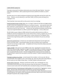
TORCS. For each of the 4096 neurons in the first fully connected layer of our direct perception CNN, we pick the top
100 images from the dataset that activate the neuron most,
and average them to get a activation pattern for this neuron. In this way, we can tell what does this neuron learn
from training. Figure 14 shows 42 typical averaged images.
We observe that the neurons’ activation patterns have strong
correlation with the host car’s heading, the location of the
lane markings and traffic cars. Thus we believe the CNN
has developed task-specific features for driving.
tem composed of 8 Support Vector Regression (SVR) and
6 Support Vector Classification (SVC) models (from libsvm
[2]) to fulfill the mapping (a mediated perception approach).
The system layout is similar to the GIST-based system (next
section) illustrated in Figure 9, but has no car perception
function.
Because the Caltech lane detector is a relatively weak
baseline, to make the task simpler, we create a special training set and testing set. Both the training set (2430 samples)
and testing set (2533 samples) are collected from the same
track (not among the 7 training tracks for CNN) without
traffic, and in a finer image resolution of 640 × 480. We discover that, even when trained and tested on the same track,
the Caltech lane detector based system still performs worse
than our model. We define our error metric as Mean Absolute Error (MAE) between the affordance estimations and
ground truth distances. A comparison of the errors for the
two systems is shown in Table 1.
3) GIST: We compare the hand-crafted GIST descriptor
with the deep features learned by the CNN’s convolutional
layers in our model. A set of 13 SVR and 6 SVC models are
trained to convert the GIST feature to the 13 affordance indicators defined in our system. The procedure is illustrated
in Figure 9. The GIST descriptor partitions the image into
4 × 4 segments. Because the ground area represented by the
lower 2 × 4 segments may be more relevant to driving, we
try two different settings in our experiments: 1) convert the
whole GIST descriptor, and 2) convert the lower 2 × 4 segments of GIST descriptor. We refer to these two baselines
as “GIST whole” and “GIST half” respectively.
Due to the constraints of libsvm, training with the full
dataset of 484,815 samples is prohibitively temporally expensive. We instead use a subset of the training set containing 86,564 samples for training. Samples in the sub training
set are collected on two training tracks with two-lane configurations. To make a fair comparison, we train another
4.2. Comparison with baselines
To quantitatively evaluate the performance of the
TORCS-based direct perception CNN, we compare it with
three baseline methods. We refer to our model as “CNN
full” in the following comparisons.
1) Behavior reflex CNN: The method directly maps an
image to steering using a CNN. We train this model on the
driving game TORCS using two settings: 1) The training
samples (over 60,000 images) are all collected while driving on an empty track; the task is to follow the lane. 2) The
training samples (over 80,000 images) are collected while
driving in traffic; the task is to follow the lane, avoid collisions by switching lanes, and overtake slow preceding cars.
For (1), the behavior reflex system can easily follow empty
tracks. For (2), when testing on the same track where the
training set is collected, the trained system demonstrates
some capability at avoiding collisions by turning left or
right. However, the trajectory is erratic. The behavior is far
different from a normal human driver and is unpredictable the host car collides with the preceding cars frequently.
2) Mediated perception (lane detection): We run the
Caltech lane detector [1] on TORCS images. Because only
two lanes can be reliably detected, we map the coordinates
of spline anchor points of the top two detected lane markings to the lane-based affordance indicators. We train a sys-
Parameter
GIST whole
GIST half
CNN sub
CNN full
angle
0.051
0.055
0.043
0.033
to LL
1.033
1.052
0.253
0.188
to ML
0.596
0.547
0.180
0.155
to MR
0.598
0.544
0.193
0.159
to RR
1.140
1.238
0.289
0.183
dist LL
18.561
17.643
6.168
5.085
dist MM
13.081
12.749
8.608
4.738
dist RR
20.542
22.229
9.839
7.983
to L
1.201
1.156
0.345
0.316
to M
1.310
1.377
0.336
0.308
to R
1.462
1.549
0.345
0.294
dist L
30.164
29.484
12.681
8.784
dist R
30.138
31.394
14.782
10.740
Table 2: Mean Absolute Error (MAE, angle is in radian, the rest are in meter) on the testing set for the GIST baseline.
5.2. Car distance estimation on the KITTI dataset
(a) Autonomous driving in TORCS
(b) Testing on real video
Figure 11: Testing the TORCS-based system. The estimation is shown as an empty box, while the ground truth is
indicated by a solid box. For testing on real videos, without
the ground truth, we can only show the estimation.
CNN on the same sub training set for 80,000 iterations (referred to as “CNN sub”). The testing set is collected by
manually driving a car on three different testing tracks with
two-lane configurations and traffic. It has 8,639 samples.
The results are shown in Table 2. The dist (car distance)
errors are computed when the ground truth cars lie within
[2, 50] meters ahead. Below two meters, cars in the adjacent
lanes are not visually present in the image. To assess how
the accuracy of dist estimation changes with distance, we
calculate errors for six different ranges and plot Figure 10.
The chosen ranges are [2,10], [2,20], [2,30], [2,40], [2,50],
and [2,60] meters.
Results in Table 2 and Figure 10 show that the CNNbased system works considerably better than the GISTbased system. By comparing “CNN sub” and “CNN full”, it
is clear that more training data is very helpful for increasing
the accuracy of the CNN-based direct perception system.
5. Testing on real-world data
5.1. Smartphone video
We test our TORCS-based direct perception CNN on real
driving videos taken by a smartphone camera. Although
trained and tested in two different domains, our system still
demonstrates reasonably good performance. The lane perception module works particularly well. The algorithm is
able to determine the correct lane configuration, localize the
car in the correct lane, and recognize lane changing transitions. The car perception module is slightly noisier, probably because the computer graphics model of cars in TORCS
look quite different from the real ones. A screenshot of the
system running on real video is shown in Figure 11b. Since
we do not have ground truth measurements, only the estimations are visualized.
To quantitatively analyze how the direct perception approach works on real images, we train a different CNN on
the KITTI dataset. The task is estimating the distance to
other cars ahead.
The KITTI dataset contains over 40,000 stereo image
pairs taken by a car driving through European urban areas.
Each stereo pair is accompanied by a Velodyne LiDAR 3D
point cloud file. Around 12,000 stereo pairs come with official 3D labels for the positions of nearby cars, so we can
easily extract the distance to other cars in the image. The
settings for the KITTI-based CNN are altered from the previous TORCS-based CNN. In most KITTI images, there is
no lane marking at all, so we cannot localize cars by the lane
in which they are driving. For each image, we define a 2D
coordinate system on the zero height plane: the origin is the
center of the host car, the y axis is along the host car’s heading, while the x axis is pointing to the right of the host car
(Figure 12a). We ask the CNN to estimate the coordinate
(x, y) of the cars “ahead” of the host car in this system.
There can be many cars in a typical KITTI image, but
only those closest to the host car are critical for driving decisions. So it is not necessary to detect all the cars. We
partition the space in front of the host car into three areas
according to x coordinate: 1) central area, x ∈ [−1.6, 1.6]
meters, where cars are directly in front of the host car. 2)
left area, x ∈ [−12, 1.6) meters, where cars are to the left
of the host car. 3) right area, x ∈ (1.6, 12] meters, where
cars are to the right of the host car. We are not concerned
with cars outside this range. We train the CNN to estimate
the coordinate (x, y) of the closest car in each area (Figure 12a). Thus, this CNN has 6 outputs.
Due to the low resolution of input images, cars far away
can hardly be discovered by the CNN. We adopt a two-CNN
structure. The close range CNN covers 2 to 25 meters (in
the y coordinate) ahead, and its input is the entire KITTI
image resized to 497 × 150 resolution. The far range CNN
covers 15 to 55 meters ahead, and its input is a cropped
KITTI image covering the central 497 × 150 area. The final
distance estimation is a combination of the two CNNs’ outputs. We build our training samples mostly form the KITTI
officially labeled images, with some additional samples we
labeled ourselves. The final number is around 14,000 stereo
pairs. This is still insufficient to successfully train a CNN.
We augment the dataset by using both the left camera and
right camera images, mirroring all the images, and adding
d
6.299
6.271
y\FP
4.332
5.000
x\FP
1.097
1.214
d\FP
4.669
5.331
Table 3: Mean Absolute Error (MAE, in meter) on the
KITTI testing set. Errors are computed by both penalizing
(column 1∼3) and not penalizing false positives (column
4∼6).
some negative samples that do not contain any car. Our final
training set contains 61,894 images. Both CNNs are trained
on this set for 50,000 iterations. We label another 2,200 images as our testing set, on which we compute the numerical
estimation error.
5.3. Comparison with DPM-based baseline
We compare the performance of our KITTI-based CNN
with the state-of-the-art DPM car detector (a mediated perception approach). The DPM car detector is provided by [5]
and is optimized for the KITTI dataset. We run the detector on the full resolution images and convert the bounding
boxes to distance measurements by projecting the central
point of the lower edge to the ground plane (zero height)
using the calibrated camera model. The projection is very
accurate given that the ground plane is flat, which holds for
most KITTI images. DPM can detect multiple cars in the
image, and we select the closest ones (one on the host car’s
left, one on its right, and one directly in front of it) to compute the estimation error. Since the images are taken while
the host car is driving, many images contain closest cars
that only partially appear in the left lower corner or right
lower corner. DPM cannot detect these partial cars, while
the CNN can better handle such situations. To make the
comparison fair, we only count errors when the closest cars
fully appear in the image. The error is computed when the
traffic cars show up within 50 meters ahead (in the y coordinate). When there is no car present, the ground truth is
set as 50 meters. Thus, if either model has a false positive,
it will be penalized. The Mean Absolute Error (MAE) for
the y and x coordinate, and the mean Euclidian distance d
between the estimated car position and the ground truth car
position are shown in Table 3. A screenshot of the system
is shown in Figure 12b.
To assess how the accuracy changes with distance on
the KITTI testing set, we calculate errors for four different
ranges and plot Figure 13. The chosen ranges are [2,20],
[2,30], [2,40], and [2,50] meters (in the y coordinate).
From Table 3 and Figure 13, we observe that our direct
perception CNN has similar performance to the state-ofthe-art mediated perception baseline. Due to the cluttered
driving scene of the KITTI dataset, and the limited number of training samples, our CNN has more false positives
than the DPM baseline on some testing samples. If we do
not penalize false positives, the CNN has much lower error
7
6
7
CNN
DPM
CNN w/o FP
DPM w/o FP
6
5
4
3
2
4
3
2
1
0
20
0
20
(a) MAE, in y
50
6
5
1
30
40
Distance threshold (meter)
7
CNN
DPM
CNN w/o FP
DPM w/o FP
Mean Euclidian diatance (meter)
x
1.565
1.502
Mean Absolute Error (meter)
y
5.832
5.824
Mean Absolute Error (meter)
Parameter
CNN
DPM + Proj.
CNN
DPM
CNN w/o FP
DPM w/o FP
5
4
3
2
1
30
40
Distance threshold (meter)
(b) MAE, in x
50
0
20
30
40
Distance threshold (meter)
50
(c) Mean distance d
Figure 13: Comparison of car distance estimation accuracy between different models. Legend: green, CNN penalizing false positives; red, DPM + Projection penalizing
false positives; dark blue, CNN not penalizing false positives; light blue, DPM + Projection not penalizing false
positives.
than the DPM baseline, which means its direct distance estimations of true cars are more accurate than the DPM-based
approach. From our experience, the false positive problem
can be reduced by simply including more training samples.
Note that the DPM baseline requires a flat ground plane
for projection. If the host car is driving on some uneven
road (e.g. hills), the projection will introduce a considerable amount of error. We also try building SVR regression
models mapping the DPM bounding box output to the distance measurements, but the regressors turn out to be far
more inaccurate than the projection, so they are not worth
comparing.
From the comparisons, we can see that, while working
on real-world images, our direct perception approach works
as well as the state-of-the-art mediated perception approach
and has a simpler structure.
5.4. Visualization of the CNN response map
To visualize how the convolutional layers of our direct
perception CNN respond to input images, we generate the
response map. In CNN, each convolutional layer is composed of a set of filters. During a forward pass, each filter convolves with the input data and generates a 2D array
(filter response). The 2D arrays generated by all the filters
of this layer share the same size. For each location in the
2D array, we take the largest value among all the filter responses to produce a single array, and it is the response map
of this convolutional layer. Location information of objects
in the original input image is preserved in the response map,
thus we can have an idea of “where does the CNN look at”
(e.g. has strong response) when making the estimation. We
show the response maps of the 4th convolutional layer of
the close range CNN on some KITTI testing images in Figure 15. We observe that the filters have strong response
over the location of the closest cars, which indicates that
the CNN learns to “look” at those cars when estimating the
distance. We further provide some response maps of our
TORCS-based CNN in Figure 16, the conclusion is similar.
Since the TORCS-based CNN is also estimating the dis-
(xm,ym)
Left area
Central
area
(-1.6m~1.6m)
(-12m~-1.6m)
(xr,yr)
Right area
y
(1.6m ~12m)
(xl,yl)
o
x
(a)
(b)
Figure 12: Car distance estimation on the KITTI dataset. (a) The coordinate system is defined relative to the host car.
We partition the space into three areas, and the objective is to estimate the coordinate of the closest car in each area. (b)
We compare our direct perception approach to the DPM-based mediated perception. The central crop of the KITTI image
(indicated by the yellow box in the upper left image and shown in the lower left image) is sent to the far range CNN. The
bounding boxes output by DPM are shown in red, as are its distance projections in the LiDAR visualization (right). The CNN
outputs and ground truth are represented by green and black boxes, respectively.
tance to lane markings, its filters have very strong response
over the location of lane markings.
6. Conclusions
In this paper, we propose a novel autonomous driving
paradigm based on direct perception. Our representation
leverages a deep CNN architecture to estimate the affordance for driving actions instead of parsing entire scenes
(mediated perception approaches), or blindly mapping an
image directly to driving commands (behavior reflex approaches). Experiments show that our system is capable
of driving a car in multiple road/traffic scenarios in a virtual
environment. Furthermore, empirical results demonstrate
that direct perception can accurately estimate many drivingrelevant affordance indicators. For future work, we plan to
collect more real-world training data to further develop our
approach. We also plan to extend our model from highways
to urban streets, and to more complex environments such as
intersections on busy roads.
Acknowledgment. This work is partially supported by
gift funds from Google, Intel Corporation and Project X
grant to the Princeton Vision Group, and a hardware donation from NVIDIA Corporation.
References
[1] M. Aly. Real time detection of lane markers in urban streets.
In Intelligent Vehicles Symposium, 2008 IEEE, pages 7–12.
IEEE, 2008. 2, 6
[2] C.-C. Chang and C.-J. Lin. Libsvm: a library for support
vector machines. ACM Transactions on Intelligent Systems
and Technology (TIST), 2(3):27, 2011. 6
[3] D. Erhan, C. Szegedy, A. Toshev, and D. Anguelov. Scalable object detection using deep neural networks. In Proceedings of the IEEE Conference on Computer Vision and
Pattern Recognition (CVPR), 2014. 3
[4] P. F. Felzenszwalb, R. B. Girshick, D. McAllester, and D. Ramanan. Object detection with discriminatively trained partbased models. Pattern Analysis and Machine Intelligence,
IEEE Transactions on, 32(9):1627–1645, 2010. 2
[5] A. Geiger, M. Lauer, C. Wojek, C. Stiller, and R. Urtasun. 3d
traffic scene understanding from movable platforms. Pattern
Analysis and Machine Intelligence (PAMI), 2014. 3, 8
[6] A. Geiger, P. Lenz, C. Stiller, and R. Urtasun. Vision meets
robotics: The kitti dataset. The International Journal of
Robotics Research, 2013. 1, 2, 3
[7] J. J. Gibson. The ecological approach to visual perception.
Psychology Press, 1979. 2
[8] R. Girshick, J. Donahue, T. Darrell, and J. Malik. Rich feature hierarchies for accurate object detection and semantic
segmentation. In Proceedings of the IEEE Conference on
Computer Vision and Pattern Recognition (CVPR), 2014. 3
[9] R. Hadsell, P. Sermanet, J. Ben, A. Erkan, M. Scoffier,
K. Kavukcuoglu, U. Muller, and Y. LeCun. Learning longrange vision for autonomous off-road driving. Journal of
Field Robotics, 26(2):120–144, 2009. 3
[10] Y. Jia, E. Shelhamer, J. Donahue, S. Karayev, J. Long, R. Girshick, S. Guadarrama, and T. Darrell. Caffe: Convolutional architecture for fast feature embedding. arXiv preprint
arXiv:1408.5093, 2014. 4
Figure 14: Activation pattern of neurons. For each of the 4096 neurons (42 shown here) in the first fully connected layer,
we pick the top 100 images that activate the neuron most, and average them to get a activation pattern for this neuron. The
neurons’ activation patterns have strong correlation with the host car’s heading, the location of the lane markings and traffic
cars.
[11] J. Koutn´ık, G. Cuccu, J. Schmidhuber, and F. J. Gomez.
Evolving large-scale neural networks for vision-based torcs.
In FDG, pages 206–212, 2013. 3
[12] A. Krizhevsky, I. Sutskever, and G. E. Hinton. Imagenet
classification with deep convolutional neural networks. In
Advances in neural information processing systems, pages
1097–1105, 2012. 3
[13] P. Lenz, J. Ziegler, A. Geiger, and M. Roser. Sparse scene
flow segmentation for moving object detection in urban environments. In Intelligent Vehicles Symposium (IV), 2011
IEEE, pages 926–932. IEEE, 2011. 2
[14] U. Muller, J. Ben, E. Cosatto, B. Flepp, and Y. L. Cun. Off-
road obstacle avoidance through end-to-end learning. In Advances in neural information processing systems, pages 739–
746, 2005. 3
[15] A. Oliva and A. Torralba. Modeling the shape of the scene: A
holistic representation of the spatial envelope. International
journal of computer vision, 42(3):145–175, 2001. 3
[16] D. A. Pomerleau. Alvinn: An autonomous land vehicle in a
neural network. Technical report, DTIC Document, 1989. 2,
3
[17] D. A. Pomerleau. Neural network perception for mobile
robot guidance. Technical report, DTIC Document, 1992.
2, 3
Figure 15: Response map of our KITTI-based CNN. The maps are generated from the responses of the 4th convolutional
layer. The level of the response is color coded, the warmer the color, the stronger the response. We observe that the filters
have strong response over the location of cars.
Figure 16: Response map of our TORCS-based CNN. The maps are generated from the responses of the 4th convolutional
layer. The level of the response is color coded, the warmer the color, the stronger the response. We observe that the filters
have strong response over the location of lane markings.
[18] S. Ullman. Against direct perception. Behavioral and Brain
Sciences, 3(03):373–381, 1980. 1
[19] P. Weinzaepfel, J. Revaud, Z. Harchaoui, and C. Schmid.
Deepflow: Large displacement optical flow with deep matching. In Computer Vision (ICCV), 2013 IEEE International
Conference on, pages 1385–1392. IEEE, 2013. 3
[20] B. Wymann, E. Espi´e, C. Guionneau, C. Dimitrakakis,
R. Coulom, and A. Sumner. TORCS, The Open Racing Car
Simulator. http://www.torcs.org, 2014. 3
[21] H. Zhang, A. Geiger, and R. Urtasun. Understanding highlevel semantics by modeling traffic patterns. In Computer Vision (ICCV), 2013 IEEE International Conference on, pages
3056–3063. IEEE, 2013. 3