
Field Observations during the Tenth Microwave Water and
AE512
Field Observations during the
Tenth Microwave Water and Energy Balance
Experiment (MicroWEX-10): from March 1, 2011,
through January 5, 20121
Tara Bongiovanni, Pang-Wei Liu, Karthik Nagarajan, Daniel Preston, Patrick Rush, Xueyang Duan,
Guanbo Chen, Robert Terwilleger, Alejandro Monsivais-Huertero, Jasmeet Judge, Roger De Roo, Ruzbeh
Akbar, Mary Morris, Olivia Williams, Lindsey Marks, Courtnay Cardozo, Mahta Moghaddam, and
Anthony England2
______________________________________________________________________________________
1.
2.
This document is AE512, one of a series of the Agricultural and Biological Engineering Department, UF/IFAS Extension. First
published April 2015. Visit the EDIS website at http://edis.ifas.ufl.edu.
Tara Bongiovanni and Pang-Wei Liu, graduate research assistants, Center for Remote Sensing (CRS), Agricultural and Biological
Engineering Department; Karthik Nagarajan, post-doctoral researcher, CRS, Agricultural and Biological Engineering Department; Daniel
Preston, engineering technician, CRS, Agricultural and Biological Engineering Department; Patrick Rush, engineer, CRS, Agricultural and
Biological Engineering Department; Xueyang Duan, Guanbo Chen, Roger De Roo, Ruzbeh Akbar, Mahta Moghaddam, and Anthony
England, Electrical Engineering and Computer Sciences Department, University of Michigan, Ann Arbor, MI 48109; Robert Terwilleger,
Lindsey Marks, and Courtnay Cardozo, undergraduate research assistants, CRS, Agricultural and Biological Engineering Department;
Alejandro Monsivais-Huertero, assistant professor, ESIME Unidad Ticomán, Instituto Politécnico Nacional, Mexico; Jasmeet Judge
([email protected]), assistant professor and director, CRS, Agricultural and Biological Engineering Department; Mary Morris and Olivia
Williams, UF Research Experience for Undergraduates; UF/IFAS Extension, Gainesville, FL 32611.
The Institute of Food and Agricultural Sciences (IFAS) is an Equal Opportunity Institution authorized to provide
research, educational information and other services only to individuals and institutions that function with nondiscrimination with respect to race, creed, color, religion, age, disability, sex, sexual orientation, marital status, national
origin, political opinions or affiliations. U.S. Department of Agriculture, Cooperative Extension Service, University of
Florida, IFAS, Florida A. & M. University Cooperative Extension Program, and Boards of County Commissioners
Cooperating. Nick T. Place, Dean.
i
TABLE OF CONTENTS
1. INTRODUCTION…………………………………………………………………………………………………………1
2. OBJECTIVES.……..………………………………………………………………………………………………………1
3. FIELD SETUP.…………………………………………………………………………………………………………….1
4. SENSORS..…………………………………………………………………………………………………………………5
4.1 University of Florida Microwave Radiometer Systems…………………………………………………………5
4.1.1 University of Florida C-band Microwave Radiometer (UFCMR)………………………………………5
4.1.1.1 Theory of operation………………………………………………………………………………7
4.1.2 University of Florida L-band Microwave Radiometer (UFLMR) ………………………………………9
4.1.2.1 Theory of operation…………………..…………………………………………………………11
4.2 University of Michigan Radiometer System……………………………………………………………………13
4.2.1 Truck Mounted Radiometer System L-band (TMRS-L)………………………………………………13
4.2.1.1 Theory of operation……………………………………………………………………………14
4.3 University of Florida Radar System…………………………………………………………………………….14
4.3.1 University of Florida L-band Automated Radar System (UF-LARS) …………………………………14
4.4 University of Michigan Radar System…………………………………………………………………………16
4.4.1 Microwave Observatory of Subcanopy and Subsurface (MOSS)……………………………………16
4.4.1.1 Theory of operation……………………………………………………………………………17
4.5 Net Radiometer…………………………………………………………………………………………………19
4.6 Air Temperature and Relative Humidity………………………………………………………………………19
4.7 Thermal Infrared Sensor ………………………………………………………………………………………20
4.7.1 Thermal Infrared Sensor (elephant grass) ………………………………………………………………20
4.7.2 Thermal Infrared Sensor (sweet corn) …………………………………………………………………20
4.8 Soil Temperature Probes ………………………………………………………………………………………20
4.8.1 Soil Temperature Probes (elephant grass) ………………………………………………………………20
4.8.2 Soil Temperature Probes (sweet corn) …………………………………………………………………21
4.9 Soil Moisture Probes ……………………………………………………………………………………………21
4.9.1 Soil Moisture Probes (elephant grass) …………………………………………………………………21
4.9.2 Soil Moisture Probes (sweet corn) ………………………………………………………………………21
4.10 Precipitation …………………………………………………………………………………………………21
4.10.1 Precipitation (elephant grass) ……………………………………………………………………………21
4.10.2 Precipitation (sweet corn) ………………………….……………………………………………………21
4.11 Drip irrigation …………………………………………………………………………………………………22
5. VEGETATION SAMPLING AT THE ELEPHANT GRASS SITE…………………………………………………22
5.1 Clump and Tiller Count ………………………………………………………………………………………22
5.2 Clump Height and Width………………………………………………………………………………………22
5.3 Tiller Height and Width…………………………………………………………………………………………23
ii
5.4 Wet and Dry Biomass ………………………………………………………………………………………….23
5.5 LAI ……………………………………………………………………………………………………………23
5.6 Vertical Distribution of Moisture in the Canopy………………………………………………………………23
5.7 Geometric Description……………………………………………………………………………………….….24
6. VEGETATION SAMPLING AT THE SWEET CORN SITE…………………………………………………………24
6.1 Height and Width………………………………………………………………………………………………24
6.2 Wet and Dry Biomass …………………………………………………………………………………………24
6.3 LAI ……………………………………………………………………………………………………………24
6.4 Vertical Distribution of Moisture in the Canopy ………………………………………………………………24
6.5 Geometric Description …………………………………………………………………………………………25
7. WELL SAMPLING………………………………………………………………………………………………………26
7.1 Water level measurement………………………………………………………………………………………26
8. SOIL SAMPLING……………………………………………………….………………………………………………26
8.1 Soil Analysis ……………………………………………………………………………………………………26
8.2 Soil Roughness …………………………………………………………………………………………………27
9. OBSERVATIONS………………..……………………………………….………………………………………………29
10. ELEPHANT GRASS FIELD LOG……………………………………………………………………………………30
11. SWEET CORN FIELD LOG…………………………………………………………………………………………37
12. REFERENCES....……………………………….………………………………………………………………………41
13. ACKNOWLEDGMENTS..……………….…………………………………………………………………………….42
A. FIELD OBSERVATIONS.………………………………………………………………………………………………43
B. JULIAN DAY CALENDAR.……………………………………………………………………………………………97
iii
1. INTRODUCTION
For accurate prediction of weather and near-term climate, root-zone soil moisture is one of the most crucial
components driving surface hydrological processes. Soil moisture in the top meter governs moisture and energy
fluxes at the land–atmosphere interface, and it plays a significant role in partitioning of precipitation into runoff and
infiltration.
Energy and moisture fluxes at the land surface during growing seasons can be estimated by coupled Soil-VegetationAtmosphere-Transfer and crop growth models. Even though the biophysics of moisture and energy transport and of
crop growth and development are well-captured in most current models, the errors in initialization, forcings, and
computation accumulate over time and the model estimates of soil moisture in the root zone diverge from reality.
Remotely sensed microwave observations can be assimilated in these models to improve root zone soil moisture and
crop yield estimates.
The microwave signatures at low frequencies, particularly at 1–4 GHz (L-band) and 4–8 GHz (C-band) are very
sensitive to soil moisture in the top few centimeters in most vegetated surfaces. Many studies have been conducted in
agricultural areas—such as bare soil, grass, soybean, wheat, pasture, and corn—to understand the relationship
between soil moisture and microwave remote sensing. It is important to know how microwave signatures vary with
soil moisture, evapotranspiration (ET), and biomass during the growing season for a dynamic agricultural canopy
with a significant wet biomass of 4–12 kg/m2.
2. OBJECTIVES
The goal of MicroWEX-10 was to conduct a season-long experiment, which incorporated active and passive
microwave observations for a growing season of elephant grass and sweet corn. The variety of sensors allowed for
further understanding of the land–atmosphere interactions during the growing season, and their effect on observed
passive microwave signatures at 6.7 GHz and 1.4 GHz and active microwave signatures at 1.14 GHz and 1.25 GHz.
These observations match that of the satellite-based passive microwave radiometers, Advanced Microwave Scanning
Radiometer-2 (AMSR-2), and the Soil Moisture and Ocean Salinity (SMOS) mission, respectively, and the upcoming
National Aeronautics and Space Administration’s Soil Moisture Active Passive (SMAP) mission. Specific objectives
of MicroWEX-10 include the following:
1. To acquire simultaneous active and passive data for both elephant grass and corn.
2. To collect passive and active microwave and other ancillary data to develop preliminary algorithms to
estimate microwave signatures for elephant grass and corn.
3. To implement alternate irrigation methods when the height of the elephant grass canopy exceeds 3 m.
4. To evaluate feasibility of soil moisture retrievals using passive microwave data at 6.7 GHz and 1.4 GHz and
active microwave data at 1.14 GHz and 1.25 GHz for the growing elephant grass canopy and corn.
This report describes the observations conducted during the MicroWEX-10.
3. FIELD SETUP
MicroWEX-10 was conducted at the UF/IFAS Extension Plant Science Research and Education Unit (PSREU), Citra,
FL. Figures 1 and 2 show the location of the PSREU and the study site for the MicroWEX-10, respectively. The study
site was located at the west side of the PSREU (29.4°N, 82.17°W). The dimensions of the elephant grass study site
were 183 m × 183 m with the corners of the field located at 29.410°N 82.179°W; 29.410°N 82.177°W; 29.409°N
82.177°W; 29.409°N 82.179°W. The elephant grass (Pennisetum purpureum) of varieties Merkeron, N-13, N-43, and
N-51, was in its second year of growth. The row spacing was 182.9 cm (72 inches). A linear move system was used
for irrigation in the beginning of the season with drip irrigation installed on May 31 (Day of Year [DoY] 151) in
2011. (See Table B-1 for corresponding months and dates to the DoY mentioned in this document on page 97.) The
instruments consisted of two ground-based microwave radiometer systems, a ground-based microwave radar system,
and micrometeorological stations. The ground-based microwave radiometer systems were installed at the location
1
shown in Figure 3(a), facing south to avoid the radiometer shadow interfering with the field of view. The groundbased microwave radar system was installed adjacent to the radiometer with a portion of the radar footprint
overlapping the radiometer footprint, facing in the same direction as the radiometer system. The ground-based
microwave radiometer systems installation began on DoY 50 in 2011 with micrometeorological stations on DoY 83
in 2011 and radar measurements starting on DoY 241 in 2011. Three micrometeorological stations with soil moisture
and soil temperature sensors were installed at the locations shown in Figure 3(a). Rain gauges were installed in line
with the outer edge of the L-band radiometer footprint. A relative humidity (RH) and temperature sensor were
installed at the C-band station. A net radiometer and thermal infrared sensor were installed south of the C-band
radiometer.
The dimensions of the corn study site were 100 m × 175 m. A linear move system was used for irrigation. The corn of
variety Yellow Supersweet Hybrid (SH2) Saturn was planted on DoY 186 in 2011, at an orientation 0º from the east.
The plant spacing was 15.9 cm (6 ¼ inches) and the row spacing was 91.4 cm (36 inches). Instrument installation
began on DoY 188 in 2011. The instruments consisted of a ground-based microwave radiometer system, two groundbased microwave radar systems, and micrometeorological stations. The ground-based microwave radiometer system
was installed at the location shown in Figure 3(b), facing south to avoid the radiometer shadow interfering with the
field of view. The ground-based microwave radar systems were installed adjacent to the radiometer with a portion of
the radar footprint overlapping the radiometer footprint, facing in the same direction as the radiometer system. Rain
gauges were installed in line with the outer edge of the radar footprint. Two micrometeorological stations with soil
moisture and soil temperature sensors were installed at the locations shown in Figure 3(b). A thermal infrared sensor
was installed in the southern end of the field out of the range of the footprints. This report provides detailed
information regarding sensors deployed and data collected during the MicroWEX-10.
Figure 1. Location of PSREU/IFAS
Credits: http://plantscienceunit.ifas.ufl.edu/directions.shtml
2
Figure 2. Location of the field site for MicroWEX-10 at the UF/IFAS PSREU
Credits: http://plantscienceunit.ifas.ufl.edu/images/location/p1.jpg
3
Figure 3(a). Layout of the sensors during MicroWEX-10 elephant grass
4
Figure 3(b). Layout of the sensors during MicroWEX-10 corn
4. SENSORS
MicroWEX-10 had six major types of instrument subsystems: (1) the ground-based University of Florida C-band and
L-band radiometers, (2) the ground-based University of Michigan L-band radiometer, (3) the ground-based
University of Florida L-band radar, (4) the ground-based University of Michigan L-band radar, (5) the
micrometeorological, and (6) the soil subsystem.
4.1 University of Florida Microwave Radiometer Systems
4.1.1 University of Florida C-band Microwave Radiometer (UFCMR)
Microwave brightness temperatures at 6.7 GHz (λ = 4.48 cm) were measured every 15 minutes using the University
of Florida’s C-band Microwave Radiometer system (UFCMR) (Figure 4[a]). The radiometer system consisted of a
dual polarization total power radiometer operating at the center frequency of 6.7 GHz housed atop a 10 m tower
installed on a 16ʹ trailer bed. The UFCMR was designed and built by the Microwave Geophysics Group at the
University of Michigan. It operates at the center frequency at 6.7 GHz, which is near one of the center frequencies on
the space borne AMSR-2 aboard the Japan Aerospace Exploration Agency’s Global Change Observation MissionWater satellite. The UFCMR observed the 6.58 m × 5.71 m footprint from a height of 7.747 m. A rotary system was
used to rotate the look-angle of the UFCMR both for field observations and sky measurements. The brightness
temperatures were observed at an incidence angle of 45˚. The radiometer was calibrated at least once every week with
a microwave absorber as warm load and measurement of sky as cold load. Figure 4(b) shows the close-up of the
rotary system and Figure 4(c) shows a close-up of the UFCMR antenna. Table 1 lists the UFCMR specifications.
Figure A-1 shows the V- and H-pol brightness temperatures observed at C-band during MicroWEX-10 for the
elephant grass field.
5
Table 1. UFCMR specifications
Parameter
Frequency
Bandwidth
Beamwidth
Qualifier
Center
3 dB
3 dB V-pol elevation a
3 dB V-pol azimuth b
3 dB H-pol elevation c
3 dB H-pol azimuth d
Isolation
Polarizations
Sequential
Receiver
temp
(Trec)
Noise Figure
From Trec
RF gain
NEDT
1 sec
8 sec
a
sidelobes < −33 dB
b
sidelobes < −28 dB
c
sidelobes < −27 dB
d
sidelobes < −35 dB
6
Value
6.7 GHz
20 MHz
23°
21°
21°
23°
> 27 dB
V/H
437 K
3.99 dB
85 dB
0.71 K
0.25 K
a
b
c
Figure 4. (a) The UFCMR system, (b) the side view of the UFCMR showing the rotary system, and (c) the front view
of the UFCMR showing the receiver antenna
Credits: J. Casanova, University of Florida
4.1.2.1 Theory of operation
The UFCMR uses a thermoelectric cooler (TEC) for thermal control of the Radio Frequency (RF) stages for the
UFCMR. This is accomplished by the Oven Industries “McShane” thermal controller. McShane is used to cool or
heat by Proportional-Integral-Derivative (PID) algorithm with a high degree of precision at 0.01°C. The RF
components are all attached to an aluminum plate that must have sufficient thermal mass to eliminate short-term
thermal drifts. All components attached to this thermal plate, including the TEC, use thermal paste to minimize
thermal gradients across junctions.
7
The majority of the gain in the system is provided by a gain and filtering block designed by the University of
Michigan for the STAR-Light instrument (De Roo 2003). The main advantage of this gain block is the close
proximity of all the amplifiers, simplifying the task of thermal control. This gain block was designed for a radiometer
working at the radio astronomy window of 1400–1427 MHz, and so the receiver is a heterodyne type with
downconversion from the C-band RF to L-band. To minimize the receiver noise figure, a C-band low-noise amplifier
(LNA) is used just prior to downconversion. To protect the amplifier from saturation due to out-of-band interference,
a relatively wide bandwidth, but low insertion loss, bandpass filter is used just prior to the amplifier. Three
components are between the filter and the antenna: a switch for choosing polarization, a switch for monitoring a
reference load, and an isolator to minimize changes in the apparent system gain due to differences in the reflections
looking upstream from the LNA.
The electrical penetrations use commercially available weatherproof bulkhead connections (Deutsch connectors or
equivalent). The heat sinks have been carefully located employing RTV (silicone sealant) to seal the bolt holes. The
radome uses 15 mil polycarbonate for radiometric signal penetration. It is sealed to the case using a rubber gasket
held down by a square retainer.
The first SubMiniature version A (SMA) connection is an electromechanical latching, driven by the Z-World control
board switches between V- and H-polarization sequentially. The SMA second latching that switches between the
analog signal from the first switch and the reference load signal from a reference load resistor sends the analog signal
to an isolator, where the signals within 6.4–7.2 GHz in radiofrequency are isolated. Then the central frequency is
picked up by a 6.7 GHz bandpass filter, which also protects the amplifier from saturation. A low-noise amplifier
(LNA) is used to eliminate the noise figure and adjust gain. A mixer takes the input from the LNA and a local
oscillator to output a 1.4 GHz signal to STAR-Light. After the power amplifier and filtering block (Star-Light backend), the signal is passed through a square law detector and a post-detection amplifier (PDA). The UFCMR is
equipped with a microcontroller that is responsible for taking measurements, monitoring the thermal environment,
and storing data until a download is requested. A laptop computer is used for running the user interface named
FluxMon to communicate with the radiometer through Radiometer Control Language (RadiCL). The radiometer is
configured to maintain a particular thermal set point, and make periodic measurements of the brightness at both
polarizations sequentially and the reference load. The data collected by the radiometer are not calibrated within the
instrument, since calibration errors could corrupt an otherwise useful dataset. Figure 5 shows the block diagram of
the UFCMR.
8
Figure 5. Block diagram of the University of Florida C-band Microwave Radiometer
Credits: De Roo (2002)
4.1.2 University of Florida L-band Microwave Radiometer (UFLMR)
Microwave brightness temperatures at 1.4 GHz (λ = 21.0 cm) were measured every 15 minutes using the University
of Florida’s L-band Microwave Radiometer system (UFLMR) (Figure 6[a]). The radiometer system consisted of a
horizontally polarized total power radiometer operating at the center frequency of 1.4 GHz housed atop a 9.14 m
tower installed on a 16ʹ trailer bed. The UFLMR was designed and built by the Microwave Geophysics Group at the
University of Michigan. It operates at the center frequency at 1.4 GHz, which is identical to the center frequency on
the space-borne SMOS mission. The UFLMR observed the 5.54 m × 4.47 m footprint from a height of 7.9375 m. The
brightness temperatures were observed at an incidence angle of 40˚. A rotary system was used to rotate the lookangle of the UFLMR for both field observations and sky measurements. The radiometer was calibrated at least every
week with a measurement of sky as cold load. Figure 6(b) shows a close up of the rotary system and Figure 6(c)
shows the antenna of the UFLMR. Table 2 lists the UFLMR specifications. Figure A-1 shows the horizontally
polarized brightness temperatures observed by the UFLMR during MicroWEX-10 for the elephant grass field.
9
a
b
c
Figure 6. (a) The UFLMR system, (b) the side view of the UFLMR showing the rotary system, and (c) the front view
of the UFLMR showing the receiver antenna
Credits: J. Casanova, University of Floida
10
Table 2. UFLMR specifications
Parameter
Frequency
Bandwidth
Beamwidth
Qualifier
Center
3 dB
3 dB H-pol elevation a
3 dB H-pol azimuth b
Single
Polarizations
Receiver
temp
(Trec)
Noise Figure
From Trec
RF gain
NEΔT
a
sidelobes < −20 dB
b
sidelobes < −30 dB
Value
1.4 GHz
20 MHz
22.5°
20.0°
H
179 K
2.1 dB
79 dB
0.5 K
4.1.2.1 Theory of operation
The UFLMR is similar to the UFCMR in many respects, using a thermoelectric cooler (TEC) for thermal control, a
similar electromechanical switching mechanism, and a Z-World controller. The PDA is the same, and the software is
a newer version of RadiCL. The RF block is designed for V- and H-pol switching. However, the UFLMR’s employs
only a single-polarization. As a result, only the H-pol signal is guided from antenna to coax to the RF block, and the
V-pol input to the RF block is a cold load (ColdFet).
In the RF block, the first switch alternates between V- and H-pol and the second alternates between the reference load
and the signal from the first switch. An isolator prevents reflections of the input signal. After the isolator, the signal
goes through a bandpass filter and then an LNA, followed by a series of bandpass filters and power amplifiers before
the square law detector and the PDA. The microcontroller logs voltage and physical temperature measurements.
Figure 7 shows the block diagram of the UFLMR.
11
Figure 7. Block diagram of the University of Florida L-band Microwave Radiometer
Credits: De Roo (2010)
12
4.2 University of Michigan Radiometer
4.2.1 Truck Mounted Radiometer System - L-band (TMRS-L)
The Truck Mounted Radiometer System (TMRS) is a dual-polarized, multi-frequency radiometer system from the
University of Michigan that measures microwave brightness temperatures. The radiometer system consisted of
multiple dual polarization total power radiometers housed atop a bucket truck. In this experiment, only the L-band
radiometer, operating at the center frequency of 1.4 GHz (λ = 21.0 cm), was used to measure every-15-minute data
(Figure 8[a]) in the corn field. The TMRS was designed and built by the Microwave Geophysics Group at the
University of Michigan. The height, incident angle, and footprint were identical to the UFLMR. A rotary system was
used to rotate the look angle of the TMRS both for field observations and sky measurements. The radiometer was
calibrated at least every week with a measurement of sky as cold load. Figure 8(b) shows the antenna and Figure 8(c)
shows the close-up of the rotary system of the TMRS-L. Table 3 lists the specifications of the TMRS-L. Figure A-2
shows the V- and H-pol brightness temperatures observed by the TMRS-L during MicroWEX-10 for the corn field.
b
a
c
Figure 8. (a) The TMRS-L, (b) the front view of the TMRS-L showing the receiver antenna, and (c) the side view of
the TMRS-L showing the rotary system
Credits: D. Preston, UF/IFAS
13
Table 3. TMRS-L specifications
Parameter
Frequency
Bandwidth
Beamwidth
Qualifier
Center
3 dB
3 dB H-pol elevation a
3 dB H-pol azimuth b
3 dB V-pol elevation c
3 dB V-pol azimuth d
Sequential
Polarizations
Receiver temp
(Trec)
Noise Figure
From Trec
RF gain
NEΔT
a
sidelobes < −20 dB
b
sidelobes < −30 dB
c
sidelobes < −30 dB
d
sidelobes < −20 dB
Value
1.4 GHz
20 MHz
22.5°
20.0°
20.0°
22.5°
V/H
179 K
2.1 dB
79 dB
0.5 K
4.2.1.1 Theory of operation
The TMRS-L is similar to the UFLMR and UFCMR in many respects, using a thermoelectric cooler (TEC) for
thermal control, a similar electromechanical switching mechanism and a Z-World controller; the PDA is the same,
and the software is an older version of RadiCL. The RF block is designed for V- and H-pol switching similar to the
UFCMR.
In the RF block, the first switch alternates between V- and H-pol and the second alternates between the reference load
and the signal from the first switch. An isolator prevents reflections of the input signal. After the isolator, the signal
goes through a bandpass filter and then an LNA, followed by a series of bandpass filters and power amplifiers before
the square law detector and the PDA. The microcontroller logs voltage and physical temperature measurements.
4.3 University of Florida Radar System
4.3.1 University of Florida L-band Automated Radar System (UF-LARS)
Observations of radar backscatter (σ0) over 21 spatial samples were collected every 15 minutes using the University
of Florida L-band Automated Radar System (UF-LARS) (Figure 9). The UF-LARS is mounted on a 25 m Genie
manlift and is comprised of three major sub-systems: (1) the antenna and the RF (ARF) sub-system, (2) the electromechanical positioning (EMP) sub-system, and (3) the software control and data acquisition (SDA) sub-system.
Figure 10 shows a simplified block diagram of the UF-LARS. The RF subsystem was based upon the established
designs for ground-based scatterometers employing a vector network analyzer with simultaneous acquisition of Vand H- polarized returns. These components operate at a center frequency of 1250 MHz, with a bandwidth of 300
MHz and the one-way 3 dB beamwidth of 14.7° in the E-plane and 19.7° in the H-plane. The polarization isolation at
the center frequency was > 37 dB for all principal planes and decreases to about 23 dB at the band edge of 1400
MHz. The EMP sub-system employs an embedded computer and is composed of three digital inclinometers, an
elevation-over-azimuth controller, linear actuators, and a laser range finder. The elevation-over-azimuth controller
was used to rotate the look-angle of the UF-LARS for both field observations and sky measurements. The antenna
incidence angle was set to 40˚. The SDA enabled system integration and automated data acquisition using a software
control system designed in the Visual C++ environment. Radar calibration included sky measurements, a trihedral
corner-reflector (Figure 9), and pole throughout the season. Table 4 summarizes the system specifications. More
information regarding the UF-LARS can be found in Nagarajan et al. (2014). Figures A-3 and A-4 show the co-pol
and cross-pol radar backscatter observed by the UF-LARS during MicroWEX-10 for the elephant grass and corn
field, respectively.
14
Figure 9. UF-LARS mounted on the 25 m Genie platform. (Inset) Trihedral calibration target made of aluminum with
an aperture length of 1.28 m.
Credits: Nagarajan et al. (2014)
Figure 10. Sub-systems within the UF-LARS
Credits: Nagarajan et al. (2014)
15
Table 4. UF-LARS specifications
Parameter
Center frequency
Bandwidth
Number of channels
Antenna HPBW
Value
1.25 GHz
300 MHz
4
14.7° (E-plane)
19.7° (H-plane)
4.4 University of Michigan Radar System
4.4.1 Microwave Observatory of Subcanopy and Subsurface (MOSS)
The Microwave Observatory of Subcanopy and Subsurface (MOSS) is an L-band tower-mounted radar (Figure 11[a])
from the University of Michigan that measures the scattering. Figure 11(b) shows the corner reflector; Figure 11(c)
shows the antennae and top-mounted electronics of the radar system; and Figure 11(d) shows its ground-mounted
electronics. This radar system operates at a center frequency of 1.14 GHz. It has two independent channels
transmitting and receiving pulses of 50 ns yielding ~20 MHz bandwidth. Polarization of each channel is determined
by the orientation of the antenna mounted. Cross-pol channels were measured by rotating one of the antennas. The
look-angle of the antennas was ~40˚, which is the same as the look angle used in the SMAP mission. The yagi
antenna used has half-power beamwidths (HPBWs) of ~32.4˚ in E-plane and ~41.4˚ in H-plane, which result in a
minimum footprint size of 12 m × 18 m (50 m × 25 m assured during the measurements) at tower height of 12 m. To
further focus the antenna beam in the vertical direction, the tower was raised stepwise from ~10 m to ~11.5 m during
each measurement, and data were taken at more than 20 locations equally spaced with a quarter-wavelength interval.
The synthesized beamwidth was ~15.3˚. Calibration of the radar system had been done in the anechoic chamber at the
University of Michigan. Sky calibration was taken before and after each full set of observations. Internal (the overall
system except the antennae) calibration was done with every datatake, and a corner reflector was measured for
absolute calibration in data post-processing. Observations of field scattering in L-band were obtained for the
morning/evening during different stages of the corn growth including germination, before ear formation, and before
harvest. Table 5 summarizes the system specifications.
Table 5. MOSS specifications
Parameter
Center frequency
Bandwidth
Number of channels
Antenna HPBW
Value
1.14 GHz
20 MHz
4
32.4° (E-plane)
41.4° (H-plane)
15.3°
Synthesized beamwidth
16
b
a
c
d
Figure 11. (a) The MOSS system, (b) corner reflector (l = 2.4157 m), (c) antennae and tower-mounted electronics,
and (d) ground-mounted electronics
Credits: X. Duan, University of Michigan
4.4.1.1 Theory of operation
Figure 12 shows a high-level system block diagram of the radar. This radar system was designed for measurements at
multiple frequencies. For this experiment the measurement frequency was specified to be 1.14 GHz. An arbitrary
waveform generator is used to produce an L-band continuous wave signal for transmit. The transmit signal is routed
through a switching network to either the V- (or 1-) or H- (or 2-) channels determined by the antenna orientation as
mounted on the tower. The transmit/receive switches (fast switches) switch at 50 ns yielding ~20 MHz bandwidth is
the radar single receive path. The network of switches that determine the transmit-and-receive paths are used to
sequentially select the channel combinations (11 12 21 22). The received signal is filtered by the L-band filter in the
17
multi-frequency bank. The received signal is then mixed down to baseband and sampled in-phase and quadrature.
The data are then stored on a PC for in-field and post analysis.
The spectral content of a returned signal from a point target is given as
E (ω ) =
G exp [−2iω r / c ]W (ω ) H (ω )σ (ω )
r2
where G is the two-way complex gain, W(ω) is the transmit pulse spectrum, H(ω) is the system frequency response
and σ(ω) is the (potentially frequency dependent) radar cross-section. For nominal field operation, it is necessary to
characterize the parameters G, W(ω), and H(ω) as a function of time and for each tower (antenna) position. The three
steps to obtain these terms in full are the internal calibration loop; the “passive,” or corner reflector calibration; and
the “active,” or transponder calibration. The internal calibration loop seen in Figure 12 characterizes the entire system
except for the antennas. Therefore, it gives W(ω), H(ω), and all of G excluding the complex antenna gain. Internal
calibration data are collected automatically at the beginning and end of every datatake (as detailed subsequently), and
the internal calibration drift can be monitored on-screen. Figure A-5 shows the radar observations during MicroWEX10.
Figure 12. Block diagram of the University of Michigan’s Microwave Observatory of Subcanopy and Subsurface
(MOSS).
Credits: X. Duan, University of Michigan
18
4.5 Net Radiometer
A Kipp and Zonen CNR-1 four-component net radiometer (Figure 13) was located in the elephant grass field, south
of the C-band radiometer (as shown in Figure 3[a]), to measure up- and down-welling shortwave and longwave
infrared radiation. The sensor consists of two pyranometers (CM-3) and two pyrgeometers (CG-3). The sensor was
installed in the elephant grass field, south of the C-band radiometer, at the height of 2.95 m above ground and facing
south on DoY 68 in 2011. On DoY 102 in 2011, the sensor was moved to a height of 4.84 m to stay above the plant
canopy. Table 6 shows the list of specifications of the CNR-1 net radiometer. Figure A-6 shows the down- and upwelling solar (shortwave) and far infrared (longwave) radiation observed during MicroWEX-10.
Figure 13. CNR-1 net radiometer
Credits: J. Casanova, University of Florida
Table 6. Specifications of the CNR-1 net radiometer
Description
Measurement spectrum: CM-3
Measurement spectrum: CG-3
Response time
Sensitivity
Pt-100 sensor temperature
measurement
Accuracy of the Pt-100 measurement
Heating
Value
305–2800 nm
5000–50000 nm
18 sec
10–35 μV/(W/m2)
DIN class A
±2K
Resistor 24 ohms, 6 VA at 12
volt
Maximum error due to heating: CM- 10 W/m2
3
Operating temperature
−40º–70ºC
Daily total radiation accuracy
± 10%
Cable length
10 m
Weight
4 kg
Source: Campbell Scientific (2006a)
4.6 Air Temperature and Relative Humidity
Air temperature and relative humidity were measured every five minutes at the C-band station in the elephant grass
field using a Campbell Scientific HMP45C Temperature and Relative Humidity Probe (Campbell Scientific 2006b).
Figure A-7 shows the relative humidity and air temperature observations during MicroWEX-10.
19
4.7 Thermal Infrared Sensor
Two Apogee instruments IRR-PN thermal infrared sensors were installed during MicroWEX-10; one in the elephant
grass and the other in the corn field site. Table 7 shows the list of specifications of the thermal infrared sensors.
Table 7. Specifications of the thermal infrared sensor (IRR-PN)
Description
Field of view
Output
Target temp.
Sensor body temp.
Accuracy
−10ºC to 65ºC
−40ºC to 70ºC
Optics
Wavelength range
Response time
Input power
Operating
environment
Cable
Dimensions
Mass
Value
18°half angle
40 μV per ºC difference
from sensor body
0–2500 mV
±0.2ºC absolute accuracy
±0.1ºC uniformity
±0.05ºC repeatability
±0.5ºC absolute accuracy
±0.3ºC uniformity
±0.1ºC repeatability and uniformity
Germanium lens
8–14 μm (corresponds to atmospheric window)
< 1 second to changes in target temperature
2.5 V excitation
−55ºC–80ºC; 0%–100% RH (non-condensing)
Water resistant, designed for continuous outdoor
use
4.5 meters twisted, shielded 4 conductor wire with
Santoprene casing.
6 cm long by 2.3 cm diameter
190 g
4.7.1 Thermal Infrared Sensor (elephant grass)
The sensor was installed south of the C-band radiometer (as shown in Figure 3[a]) at a height of 2.5 m to observe
skin temperature at nadir. On DoY 102 in 2011, the sensor was raised to 4.8 m. Figure A-8 shows the thermal
infrared temperatures observed during MicroWEX-10.
4.7.2 Thermal Infrared Sensor (sweet corn)
The sensor was installed south of the radar and radiometer footprints (as shown in Figure 3[b]) at a height of 2.245 m
to observe skin temperature at nadir. Figure A-9 shows the surface thermal infrared temperature observed during
MicroWEX-10.
4.8 Soil Temperature Probes
Lab made temperature probes, based on Campbell Scientific 107-l temperature sensor, were used to measure soil
temperature.
4.8.1 Soil Temperature Probes (elephant grass)
Thirty-nine temperature probes were placed at depths of 2, 4, 8, 16, 32, 64, 100, 120, and 150 cm measuring every
five minutes. At the C-band and L-band stations, the depths included replicates at 2, 4, 8, 16, and 32 cm. The radar
station included two replicates at 2, 4, and 8 cm. Figure A-10 shows the soil temperatures observed at the depths of 2,
4, 8, 16, 32, 64, 120, and 150 cm at the L-band station during MicroWEX-10. Figure A-11 shows the soil
temperatures at the same depths at the C-band station during MicroWEX-10. Figure A-12 shows the soil
temperatures observed at the depths of 2, 4, 8, 16, 32, 64, and 100 cm at the radar station during MicroWEX-10.
20
4.8.2 Soil Temperature Probes (sweet corn)
Twenty-six temperature probes were placed at depths of 2, 4, 8, 16, 32, 64, and 100 cm measuring every five
minutes. The north and the south station included 2 replicates at 2, 4, and 8 cm. Figure A-13 and Figure A-14 show
the soil temperatures observed at the depths of 2, 4, 8, 16, 32, 64, and 100 cm at the north and south station,
respectively, during MicroWEX-10.
4.9 Soil Moisture Probes
Campbell Scientific time-domain water content reflectometers (CS616) were used to measure soil volumetric water
content. The calibration coefficients were obtained from laboratory calibration and are listed in Table 8.
Table 8. The calibration coefficients for the CS616 probe
Coefficient
C0
C1
C2
C3
Value
1.5377
0.1814
−0.0070
0.0001
4.9.1 Soil Moisture Probes (elephant grass)
Thirty-nine reflectometers were placed at depths of 2, 4, 8, 16, 32, 64, 100, 120, and 150 cm measuring every five
minutes. At the C-band and L-band stations, the depths included replicates at 2, 4, 8, 16, and 32 cm. The radar station
included two replicates at 2, 4, and 8 cm. Figure A-15 shows the volumetric soil moisture contents observed at the
depths of 2, 4, 8, 16, 32, 64, 120, and 150 cm at the L-band station during MicroWEX-10. Figure A-16 shows the
volumetric soil moisture contents observed at the same depths at the C-band station during MicroWEX-10. Figure A17 shows the volumetric soil moisture contents observed at the depths of 2 cm, 4 cm, 8 cm, 16 cm, 32 cm, 64 cm, and
100 cm at the Radar station during MicroWEX-10.
4.9.2 Soil Moisture Probes (sweet corn)
Twenty-six reflectometers were placed at depths of 2, 4, 8, 16, 32, 64, and 100 cm measuring every five minutes. The
north and the south station included two replicates at 2, 4, and 8 cm. Figure A-18 and Figure A-19 shows the
volumetric soil moisture contents observed at the depths of 2, 4, 8, 16, 32, 64, and 100 cm at the north and south
station, respectively, during MicroWEX-10.
4.10 Precipitation
Precipitation and overhead irrigation was determined using six tipping-bucket rain gauges with locations shown in
Figure 3(a) and (b).
4.10.1 Precipitation (elephant grass)
Two tipping-bucket rain gauges, in line with the outer edge of the L-band radiometer footprint were installed on DoY
129 in 2011 at a height of 20 cm above the ground to catch both precipitation and irrigation. Figure A-20 shows the
observed precipitation and overhead irrigation.
4.10.2 Precipitation (sweet corn)
Four tipping-bucket rain gauges, in line with the outer edge of the Michigan radiometer footprint and at the southeast
and southwest corners of the field were installed on DoY 193 in 2011 at a height of 20 cm. The rain gauges were
raised to a height of 3 m above the ground on DoY 224 in 2011 to stay above the height of the corn canopy. Figure
A-21 shows the observed precipitation.
21
4.11 Drip Irrigation
Drip-tape with a diameter of 15.9 mm (⅝ inch) and emitters every 30.5 cm (12 inches) was installed on DoY 151 in
2011 in the elephant grass field (Figure 14). The specified flow rate was 0.5 gpm/100 ft. In the north side of the field,
where intensive monitoring was typically conducted, three drip tapes per row were installed (Figure 14). In other
areas of the field, one drip tape per row was installed. Drip irrigation occurred on DoY 209, DoY 217, DoY 220,
DoY 230, DoY 245, DoY 256, DoY 278, and DoY 280 in 2011. On DoY 4 and DoY 5 in 2012, measurements were
taken using a flow meter in six locations of the field. Figure A-22 shows the observed flow measurements.
Figure 14. Irrigation via drip-tape
Credits: D. Preston, UF/IFAS
5. VEGETATION SAMPLING AT THE ELEPHANT GRASS SITE
Vegetation properties in four spatially distributed sampling locations, as shown in Figure 3(a), were measured from
DoY 74 until DoY 312 in 2011 during the field experiment. The first sampling occurred in all four locations of the
field on DoY 74 in 2011. Starting on DoY 111 in 2011 biweekly sampling occurred until DoY 279 in 2011 with a
sampling in the northern sections of the field on DoY 312 and DoY 342 in 2011. A vegetation sampling consisted of
measurements of clump height and width, as well as tiller height, width, biomass, LAI, and geometric description of
the plant. Vertical distribution of moisture in the canopy was also measured when the canopy reached 4.5 m. Two
sampling locations were located where Merkron was planted in the north end of the field, while the other sampling
locations included N-51 in the southwest location and N-13 in the southeast location of the field. Each sampling
included one row of elephant grass in the four sampling locations. The sampling length started between two clumps
and ended at the next midpoint between clumps that was greater than or equal to 4 m from the starting point.
5.1 Clump and Tiller Count
The clumps and tillers were counted for each sampling length in each of the four sampling areas. Before DoY 181 in
2011, when the tillers were not uniform in height, three representative clumps were chosen to determine the
percentages of small, medium, and large tillers in the sampling area. Figure A-23 and A-24 show the clumps and
tillers per square meter.
5.2 Clump Height and Width
Maximum clump height and width were measured by placing a tape measure at the soil surface adjacent to the stems
to the maximum height of the clump. The clump width, parallel to the row, was measured at the base of the clump.
Before DoY 209 in 2011, all clump heights and widths were measured in the sampling area described in 5.1. From
DoY 209 in 2011 until the end of the season, measurement of the maximum clump height was taken from 1–3 sample
clumps. Figures A-25 and A-26 show the average of the maximum clump heights and widths during MicroWEX-10.
22
5.3 Tiller Height and Width
One to three representative tillers were selected from the 10 sample tillers to obtain heights and widths. Tiller height
and width were measured by placing a tape measure at the soil surface adjacent to the stem up to the maximum height
of the crop. The maximum width of the tiller (parallel or perpendicular to the row) was also measured. Figures A-27
and A-28 show the maximum tiller height and width during MicroWEX-10.
5.4 Wet and Dry Biomass
Using the sampling area, 10 tillers each of representative small, medium, and large were chosen from the three
clumps in section 5.1. Each tiller was cut at the base, separated into leaves and stems, and weighed immediately. The
samples were dried in the oven at 60ºC for one week for leaves and two weeks for stems. Figure A-29 shows the wet
and dry biomass (in kg/m2) observed during MicroWEX-10 for the four sampling areas.
5.5 LAI
LAI was measured with destructive sampling implementing Equation 1. Using the 1–3 tillers selected in section 5.3,
the leaves were separated from the stems. The length and width of the green leaves were measured. The specific leaf
area (SLA) in Equation 1 was calculated, assuming a leaf as an ellipse (Boote 1994). The green leaves, senesced
leaves, and the stems were then dried in an oven at 60°C for 48–72 hours to measure the dry weight of the leaves and
the dry biomass of the sample. The ratio of the leaf dry weight to the sample dry biomass was used to calculate the
fraction of leaf (FLEAF). The total dry biomass (DM) was obtained in section 5.4.
𝐿𝐿𝐿𝐿𝐿𝐿 = 𝐷𝐷𝐷𝐷 ∙ 𝐹𝐹𝐿𝐿𝐿𝐿𝐿𝐿𝐿𝐿 ∙ 𝑆𝑆𝑆𝑆𝑆𝑆
(Equation 1)
The LAI obtained is shown in Figure A-30.
5.6 Vertical Distribution of Moisture in the Canopy
The vertical distribution measurement was conducted on DoY 270 in 2011 during MicroWEX-10. The sampling
consisted of one representative tiller from the northwest area. The tiller was cut at the base and laid with the leaves
arranged to closely match their natural orientation in the field as shown in Figure 15. The tiller was cut every 20 cm.
The sample in each layer was weighed, both fresh and after drying in the oven at 60°C for 48 hours. Figure A-31
shows the wet and dry weights as a function of crop height during MicroWEX-10.
Figure 15. Tiller sample marked and ready to be subdivided into 20 cm layers
Credits: T. Bongiovanni, UF/IFAS
23
5.7 Geometric description
A geometric description of the tiller consisted of the leaf height from the ground and the maximum length and width
of each green leaf of the 1–3 representative tillers in section 5.3. The stem circumference was measured by using a
string to wrap around the base and around the tip of the plant to calculate the diameter of the stem. The stem length
was measured from the base of the tiller to the base of the last leaf. Figure A-32 (a–b) shows the height of each leaf.
The leaf length and width are shown in Figures A-33 (a–b) and A-34 (a–b). The stem length and diameter observed
are shown in Figure A-35 and A-36.
6. VEGETATION SAMPLING AT THE SWEET CORN SITE
Vegetation properties in two sampling locations as shown in Figure 3(b) were measured weekly during the field
experiment. A vegetation sampling consisted of measurements of height, width, biomass, LAI, geometric description
of the plant, and vertical distribution of moisture in the canopy. The crop density derived from the stand density (6.3
plants per m2) and row spacing (36″) was measured at the first sampling (DoY 196). The first two vegetation
sampling on DoY 196 and DoY 200 in 2011 did not include measurements of moisture distribution in the canopy or
stem diameter. After the initial two vegetation samplings, seven vegetation samplings were conducted on DoY 207,
DoY 214, DoY 221, DoY 229, DoY 236, DoY 243, and DoY 250 in 2011.
6.1 Height and Width
Crop height and width were measured by placing a measuring stick at the soil surface adjacent to the stem up to the
maximum height of the crop. The maximum canopy width of the plant (parallel or perpendicular to the row) was also
measured. Four representative plants were selected to obtain heights and widths inside each vegetation sampling area.
Figure A-37 shows the average maximum crop heights and widths during MicroWEX-10.
6.2 Wet and Dry Biomass
Each sampling included one row of corn in the four sampling locations. The sampling length started between two
plants and ended at the next midpoint between plants that was greater than or equal to one meter away from the
starting point. The plants within this length were cut at the base, separated into leaves, stems, and ears, and weighed
immediately. The samples were dried in the oven at 60ºC for one week and weighed. Figure A-38 shows the wet and
dry biomass observed during MicroWEX-10 for the four sampling areas.
6.3 LAI
Destructive LAI was measured by taking two representative plants in the sampling area and separating the leaves.
The leaves and the rest of the plant were then dried in an oven at 60°C for one week to measure the dry weight of the
leaf and the dry biomass of the sample. The ratio of the leaf dry weight to the dry biomass was used to calculate the
fraction of leaf (FLEAF) in Equation 1. The length and width of each individual leaf of the four sample plants were also
measured. Assuming a leaf as an ellipse, the area of the leaves was summed and divided by the dry mass of the leaves
to calculate the specific leaf area (SLA) in Equation 1. The total dry biomass (DM) was found using the procedure in
5.2. Equation 1 was then used to determine the destructive LAI (Boote 1994). The LAI obtained is shown in Figure
A-39.
6.4 Vertical Distribution of Moisture in the Canopy
The wet and dry biomass of discrete vertical layers of individual corn plants was measured. Seven samplings were
conducted during MicroWEX-10. Each sampling was conducted by selecting a representative plant at each sampling
location. The plants were taken out of the ground with the roots still attached and taken indoors to prevent moisture
loss. Each plant sample was carefully laid out on a metal sheet with grid spacing of 2 cm. The leaves were arranged
to closely match their natural orientation in the field. The stem was cut every 10 cm as shown in Figure 16. The
sample in each layer was weighed, both fresh and after drying in the oven at 60°C for 48 hours. Figure A-40 shows
the wet and dry weights as a function of crop height during MicroWEX-10.
24
Figure 16. Subdividing plant samples into 10 cm layers
Credits: D. Preston, UF/IFAS
6.5 Geometric description
A geometric description of the plant consisted of the maximum length and width of each leaf of the sample plants, as
shown in Figure 17. The stem circumference was measured by using a string to wrap around the base and around the
tip of the plant to calculate the diameter of the stem. The ear length was measured while still in the husk from the
base of the cob near the stem to the top, and the maximum circumference of the ear was measured by using a string.
The stem length and diameter observed are shown in Figure A-41. Figure A-42 shows the height of each leaf. The
leaf length and width are shown in Figures A-43 and A-44. The ear height, length, and diameter are shown in Figure
A-45. The ear and leaf angles were measured from a digital photograph of a single plant taken while still in the field
at each sampling area using a reference length such as a meter stick. The angle between the leaf and the stem (θ1), the
angle of the leaf fold (θ2), and the ear angle (θe) were measured using an angle gage, as shown in Figure 18. See
Figures A-46 and A-47 for the value of θ1 and θ2. Figure A-48 shows the ear angle for each ear.
Leaf width
Leaf length
Figure 17. Leaf length and width
Credits: D. Preston, UF/IFAS
25
Figure 18. Leaf angles and ear angle location
Credits: R.Terwilleger, UF/IFAS
7. WELL SAMPLING
7.1 Water level measurement
The water level measurement was processed by the Levelogger from Solinst Canada Ltd. The Leveloggers were
installed at the northern wells in the elephant grass field and set to automatically record the water level every 30
minutes. The data were downloaded onto a laptop during the well sampling. Figure A-49 shows the water table
elevation and depth during MicroWEX-10.
8. SOIL SAMPLING
8.1 Soil Analysis
Soil sampling from two locations in the corn field and two locations in the elephant grass field was done on DoY 174
in 2011 and from four locations of the elephant grass field on DoY 208 in 2011. Samples included organic matter,
texture analysis, and full (10, 18, 32, 56, 100, 316, 1000, and 1500 kPa) and partial (10 and 1500 kPa) moisture
curves from depths of 1–10, 10–40, 40–90, and 90–120 cm for the corn field and 0–15, 15–40, 40–70, and 70–100
cm for the elephant grass site (Figure A-50). The texture analysis was conducted at the elephant grass field site for
depths of 0–10 cm for two locations and 0–15 cm for four locations of the field (Table 9). The texture analysis was
conducted at the corn field site for depths of 0–10 cm in two locations of the field (Table 10). Organic matter, bulk
density, and saturated hydraulic conductivity in the elephant grass field was conducted for depths of 0–15, 15–40, 40–
70, and 70–100 cm for four locations in the field. Organic matter and saturated hydraulic conductivity in the corn
field was conducted for depths of 0–10, 10–40, and 40–90 cm for one location and 0–10, 10–40, 40–90, and 90–120
cm for the other location in the field. Bulk density in the corn field was conducted twice for depths of 0–10, 10–40,
and 40–90 cm for one location and 0–10, 10–40, 40–90, and 90–120 cm for the other location in the field.
26
Table 9. The soil physical properties for elephant grass field site (percentages are given on a weight basis)
Elephant Grass Soil Physical Properties
Sand (%)
Silt (%)
Depth
0–10
0–15
15–40
40–70
Avg
94.360
92.443
-
SD
0
0.688
-
Avg
2.000
2.668
-
70–100
-
-
-
Clay (%)
SD
Avg
0
3.64
0.471 4.890
-
-
OM (%)
KSAT
(cm/hr)
Bulk Density
(g/cm3)
SD
0
0.500
-
Avg
2.268
2.248
1.310
SD
0.676
0.662
0.633
Avg
527
102
276
SD
456
43
82
Avg
1.416
1.630
1.497
SD
0.165
0.088
0.194
-
1.115
0.630
277
73
1.395
0.112
Table 10. The soil physical properties for the corn field site (percentages are given on a weight basis)
Corn Soil Physical Properties
Sand (%)
Depth
0–10
10–40
40–90
90–120
Avg
93.525
-
SD
1.181
-
Silt (%)
Avg
SD
2.335 0.474
-
Clay (%)
Avg
4.140
-
SD
0.707
-
OM (%)
Avg
1.505
1.625
0.620
0.790
SD
0.049
0.233
0.113
-
KSAT
(cm/hr)
Avg
100
95
127
152
SD
36
45
0
-
Bulk Density
(g/cm3)
Avg
1.515
1.689
1.544
1.632
SD
0.178
0.033
0.164
0.085
8.2 Soil Surface Roughness
Soil roughness was measured near the radiometer footprints in the corn field on DoY 160, 162, 182, 200, 227, and
231 in 2011 with a traditional grid board method (Table 11). The 2D surface profiles in directions parallel and
perpendicular to the row structure were measured using a 2 m long grid board. Jang et al. (2005) describes the grid
board method in detail. Table 12 lists the root mean square height and correlation length measurements parallel and
perpendicular to the row structure.
27
Table 11. Soil surface roughness measurements using 2 m long grid board
DoY (2011)
Parellel to row structure
160
Before Plowing
-
160
After Plowing
-
162
-
Perpendicular to row structure
182
Before Plowing
182
After Plowing
200
227
231
28
Table 12. Soil surface roughness measurements of root mean square height (s) and correlation length (cl)
DoY
160
Before Plowing
160
After Plowing
162
182
Before Plowing
182
After Plowing
200
227
231
Parallel to row structure
s (cm)
cl (cm)
Perpendicular to row structure
s (cm)
cl (cm)
-
-
0.78
7.40
-
-
1.30
6.91
-
-
1.60
7.62
0.25
20.44
0.66
20.92
0.90
13.40
1.74
8.76
0.41
0.86
0.42
13.69
11.95
9.95
1.07
0.62
0.69
12.57
13.88
14.98
9. OBSERVATIONS
For the microwave radiometric observations at C-band, the horizontally polarized brightness temperatures were found
to be more sensitive to soil moisture than vertically polarized brightness temperatures during the short vegetation
cover periods (Figure A-1). As the vegetation grew, it effectively masked the contribution of microwave emission
from soil resulting in sensitivity decrease at both polarizations. Due to its higher penetration capability, the
observations at lower frequencies (longer wavelengths), such as the L-band, were more sensitive to soil moisture
during the growing season than at the higher frequencies of C-band (Figure A-2). The σ0VV was more sensitive to the
vertical structure of growing vegetation in the mid- and late-stages of crop growth (Figure A-3–A-4).
The first row in Figure A-5 shows the measurements of the field of germinating corn. The signature of the return
signal does not change much from the bare soil measurements, as expected. The second row in Figure A-5 presents
the measurements of the field when the corn grew approximately 1 meter tall before earing. More features appear in
the return signals even after 600 ns. Both the HH and VV measurements show larger ground return signals. The cross
polarization components are also measured, showing similar signature as the co-pol components. This becomes
clearer in the third row of Figure A-5, showing the measurements of the corn field right before harvest.
The average down-welling shortwave radiation average was 206.22 W/m2 during the growing season while the
average up-welling shortwave radiation was 38.93 W/m2 (Figure A-6). The average relative humidity was 79.89%
while the average air temperature was 294.76 K (Figure A-7). The average thermal infrared temperature was 287.70
K and 300.78 K for the elephant grass and corn field, respectively (Figure A-8–A-9). The rain gauges below the
canopy in the elephant grass field tended to give diverse readings, which could be due to canopy cover (Figure A-20–
A-21). Figure A-22 shows that the flow meter measurements of the drip tape were highest at the main line and
decreased as the drip tape went into the field. The water table gradually decreased as the year progressed (Figure A49). The field capacity (10 kPa) for the elephant grass field site was higher than the corn site; however, the wilting
point (1500 kPa) was similar (Figure A-50).
During the beginning of the season when vegetation was low, diurnal variations in soil temperature were maximum,
while later in the season the diurnal variations were minimal. Diurnal variations for soil temperatures at 64 cm and
below were minimal throughout the season (Figure A-10–A-14). The change in soil moisture in the deeper layers was
minimal during light rains (Figure A-15–A-19).
29
The average clump density for the elephant grass was 0.9 clump/m2 (Figure A-23). The tiller density started high
before decreasing and reaching equilibrium (Figure A-24). The maximum height of the canopy was the highest at the
NW vegetation sampling area, reaching 5.3 m, while the NE and SW area were the lowest, with a maximum height of
4.2 m (Figure A-25). The average clump width was 0.42 m (Figure A-26). The maximum height of the sample tillers
was the highest at the NW vegetation sampling area, reaching 5.4 m, while the NE area was the lowest, with a
maximum height of 4.0 m (Figure A-27). The widest maximum width of the sample tiller was an average of 2.22 m
for the SW vegetation sampling areas (Figure A-28). The biomass of the plant increased before reaching a maximum
and then decreased slightly (Figure A-29). The LAI increased before reaching a maximum of 12.7 m2/m2, and then
decreased due to leaf senescence (Figure A-30). The moisture per 10 cm section in the plant remained relatively
constant due to the stem until there was a decrease with the lowest amount of moisture located at the top of the plant
(Figure A-31). The maximum number of leaves in the NE vegetation sampling area was 38 leaves, while the SE
vegetation sampling area had a maximum of 62 leaves due to the increased number of tillers (Figure A-32). The
maximum leaf length was 1.46 m (Figure A-33) and the maximum leaf width was 0.055 m (Figure A-34). The length
of the stem increased until DoY 200 when it leveled out (Figure A-35). The average minimum diameter was 0.012 m,
while the average maximum diameter was 0.018 m (Figure A-36).
The maximum height of the sweet corn was the same for both vegetation sampling area, reaching 1.7 m (Figure A37). The maximum width of the sweet corn plant was 0.95 m at the north vegetation sampling areas (Figure A-37).
The biomass of the plant continued to increase in the south sampling area while the biomass in the north sampling
area reaching an equilibrium after DoY 236 in 2011 (Figure A-38). The LAI increased before reaching a maximum of
3 m2/m2, and then decreasing slightly due to leaf senescence (Figure A-39). During ear formation the moisture per 10
cm section in the plant was higher at the ear location (Figure A-40). The length of the stem increased until DoY 236
in 2011 when it leveled out (Figure A-41). The average minimum diameter was 0.009 m while the average maximum
diameter was 0.023 m (Figure A-41). The maximum number of leaves in the south vegetation sampling area was 20
(Figure A-42). The maximum leaf length was 0.84 m (Figure A-43) and the maximum leaf width was 0.095 m
(Figure A-44). Each plant had 1–2 ears, with the highest ear not exceeding 0.60 m above the base (Figure A-45). The
ear located highest on the plant was bigger in both length and diameter than the other ears on the plant (Figure A-45).
For the leaf angles, θ1 ranged from 0°–90° from the vertical (Figure A-46) while θ2 ranged from 90°–180° (Figure A47). The ear angle, θe, was larger for the bigger ears (Figure A-48).
10. ELEPHANT GRASS FIELD LOG
Note: Time is in Eastern Standard Time.
March 1 (DoY 60)
Buried L-band station sensor 2–32 cm north pit
Marked vegetation sampling areas in 60ʹ–75ʹ (10 rows × 75ʹ)
L-band radiometer was mounted (looking angle 45°)
Marked L-band footprint
March 2 (DoY 61)
8:50
Attached guy wires to C-band
Installed L-band station pole
March 4 (DoY 63)
Timer of L-band radiometer fixed
March 7 (DoY 66)
9:45
Buried L-band station sensor 2–150 cm south pit
30
March 9 (DoY 68)
Installed CNR at 2.95 m
Installed TIR pole
Installed low rain gauges
Buried C-band station soil sensors
March 15 (DoY 74)
Elephant grass vegetation sampling
March 22 (DoY 81)
Took L-band radiometer out of field to burn
Removed sensors from field
April 12 (DoY 102)
Reburied sensors
April 18 (DoY 108)
L-band radiometer mounted (looking angle 40°)
April 21 (DoY 111)
Elephant grass vegetation sampling NE and NW
April 25 (DoY 115)
9:45
L-band radiometer calibration
May 4 (DoY 124)
10:00
L-band radiometer calibration
May 5 (DoY 125)
Elephant grass vegetation sampling NE, NW, SE, and SW
May 6 (DoY 126)
C-band radiometer mounted (angle 90°)
May 9 (DoY 129)
C-band radiometer error msg: overheat shutdown
Hooked by C-band radiometer rotator
Installed NE and NW rain gauges
May 11 (DoY 131)
14:50
L-band radiometer calibration
May 12 (DoY 132)
14:50
C-band radiometer troubleshooting
May 13 (DoY 133)
Rebooted C-band radiometer
Adjusted gain and offset for C-band radiometer
May 16 (DoY 136)
10:35
L-band radiometer calibration
Adjusted gain and offset for C-band radiometer
C-band radiometer calibration
31
May 17 (DoY 137)
10:35
L-band radiometer calibration
May 19 (DoY 139)
10:35
L-band radiometer calibration
Elephant grass vegetation sampling NE, NW, SE, and SW
May 24 (DoY 144)
14:30
C-band radiometer calibration
15:20
L-band radiometer calibration
TIR pole knocked down
Measured CNR height: 4.84 m
May 31 (DoY 151)
Installed drip tape
Lowered CNR
Raised CNR
June 1 (DoY 152)
9:40
C-band radiometer calibration
10:20
L-band radiometer calibration
12:00
Lowered CNR
June 2 (DoY 153)
Elephant grass vegetation sampling NE, NW, SE, and SW
10:00
Raised CNR
12:00
Lowered CNR
June 3 (DoY 154)
Raised CNR
June 7 (DoY 158)
10:35
C-band radiometer calibration
11:20
L-band radiometer calibration
10:00
Lowered CNR
June 8 (DoY 159)
13:30
Raised CNR
June 9 (DoY 160)
10:15
C-band radiometer calibration
11:03
L-band radiometer calibration
June 16 (DoY 167)
9:10
C-band radiometer calibration
10:05
L-band radiometer calibration
Elephant grass vegetation sampling NE, NW, SE, and SW
June 23 (DoY 174)
9:25
C-band radiometer calibration
10:20
L-band radiometer calibration
June 29 (DoY 180)
10:00
L-band radiometer calibration
10:50
C-band radiometer calibration
32
June 30 (DoY 181)
8:30
Elephant grass vegetation sampling NE, NW, SE, and SW
July 7 (DoY 188)
11:25
C-band radiometer calibration
12:20
L-band radiometer calibration
July 14 (DoY 195)
10:30
C-band radiometer calibration
11:16
L-band radiometer calibration
Elephant grass vegetation sampling NE, NW, SE, and SW
July 21 (DoY 202)
9:20
C-band radiometer calibration
10:05
L-band radiometer calibration
July 26 (DoY 207)
Replaced C-band station 8 cm and 32 cm thermistors with new model in north pit
Fixed two TDRs on C-band station
July 27 (DoY 208)
Soil sampling in elephant grass field in skip row
July 28 (DoY 209)
8:50
Elephant grass vegetation sampling NE, NW, SE, and SW
9:00
C-band radiometer calibration
10:05
L-band radiometer calibration
9:25
Drip tape turned on
August 2 (DoY 214)
Replaced C-band station 2, 4, and 16 cm thermistors with new model in north pit
Connected C-band-thermistors
August 4 (DoY 216)
9:17
L-band radiometer calibration
10:17
C-band radiometer calibration
Replaced L-band station 64 and 120 cm thermistors
C-band 32 cm thermistor output writing to wrong array
August 5 (DoY 217)
7:30
Drip irrigation ~ 5 hrs
Fixed hole in drip irrigation at C-band north pit
August 8 (DoY 220)
Drip irrigation ~ 24 hrs
August 11 (DoY 223)
Elephant grass vegetation sampling NE, NW, SE, and SW
August 12 (DoY 224)
9:16
L-band radiometer calibration
9:32
C-band radiometer calibration
Power failure in evening
33
August 18 (DoY 230)
Drip Irrigation
9:06
C-band radiometer calibration
9:36
L-band radiometer calibration
August 25 (DoY 237)
Elephant grass vegetation sampling NE, NW, SE, and SW
C-band was set to incident angle of 52° changed back to 45°
August 26 (DoY 238)
8:47
C-band radiometer calibration
9:18
L-band radiometer calibration
Moved radar to elephant grass field
August 28 (DoY 240)
Radar stopped
August 29 (DoY 241)
Restarted radar
Cleared skip row to get to radar center
Buried sensors for radar station
August 30 (DoY 242)
Stopped radar to look for laser height
Restarted radar
August 31 (DoY 243)
Set up pole with board for height measurement
14:45
Radar stopped working
September 1 (DoY 244)
Radar calibration
September 2 (DoY 245)
Brought radar down to work on restart
Drip irrigation
September 6 (DoY 249)
Power failure
September 7 (DoY 250)
9:35
C-band radiometer calibration
10:15
L-band radiometer calibration
Switched UPS battery
Moved radar to corn field
September 8 (DoY 251)
Elephant grass vegetation sampling NW and SW
September 13 (DoY 256)
Drip irrigation ~5 hrs
Wired in radar station, started program
34
September 15 (DoY 258)
9:20
C-band radiometer calibration
9:50
L-band radiometer calibration
Moved radar to elephant grass field
Fixed thermistors on L-band station- found corrosion
September 20 (DoY 263)
9:28
Michigan radiometer calibration
Moved Michigan radiometer to elephant grass field
Power failure on C-band and L-band radiometer
September 21 (DoY 264)
9:24
C-band radiometer calibration
9:50
L-band radiometer calibration
10:20
Michigan radiometer calibration
September 22 (DoY 265)
Elephant grass vegetation sampling NW and SW
September 27 (DoY 270)
9:27
L-band radiometer calibration
10:20
C-band radiometer calibration
Michigan radiometer power failure
Unplugged Michigan radiometer’s UPS
Michigan radiometer calibration
Radar stopped
September 30 (DoY 273)
Michigan radiometer power failure
October 3 (DoY 276)
Changed the GFI breaker to normal for Michigan radiometer
October 5 (DoY 278)
Drip irrigation ~5 hrs
October 6 (DoY 279)
11:32
L-band radiometer calibration
C-band radiometer calibration
Michigan radiometer calibration
Elephant grass vegetation sampling NW and SW
October 7 (DoY 280)
Drip irrigation ~5 hrs
October 10 (DoY 283)
Power failure
Restarted radiometers
October 11 (DoY 284)
Restarted radar
35
October 13 (DoY 286)
Radar failed
Michigan radiometer calibration
9:25
L-band radiometer calibration
10:12
C-band radiometer calibration
October 17 (DoY 290)
14:57
Michigan radiometer calibration
October 20 (DoY 293)
9:47
Michigan radiometer calibration
9:50
L-band radiometer calibration
10:47
C-band radiometer calibration
October 24 (DoY 297)
14:50
Michigan radiometer calibration
October 27 (DoY 300)
9:35
C-band radiometer calibration
9:53
Michigan radiometer calibration
Power for truck failed
L-band radiometer calibration
October 28 (DoY 301)
14:46
Michigan radiometer calibration
Michigan radiometer rotator failed
November 3 (DoY 307)
9:58
L-band radiometer calibration
10:35
C-band radiometer calibration
November 8 (DoY 312)
Elephant grass vegetation sampling NE and NW
November 10 (DoY 314)
9:06
C-band radiometer calibration
9:47
L-band radiometer calibration
November 17 (DoY 321)
Radar stopped
1:55
L-band radiometer calibration
2:32
C-band radiometer calibration
South flowering completed
North ready to flower
Fixed station time
Michigan rotator fixed
Michigan radiometer calibration
November 22 (DoY 326)
9:10
Michigan radiometer calibration
9:10
L-band radiometer calibration
9:47
C-band radiometer calibration
36
November 25 (DoY 329)
Radar not moving
17:33
Connected and restarted radar
December 6 (DoY 340)
Radar not moving
10:00
L-band radiometer calibration
10:05
Michigan radiometer calibration
10:32
C-band radiometer calibration
11:32
Restarted radar
December 8 (DoY 342)
Elephant grass vegetation sampling NE and NW
Started to remove sensors
December 19 (DoY 353)
9:18
C-band radiometer calibration
10:02
L-band radiometer calibration
Uninstalled C-band radiometer
January 4 (DoY 4)
Drip tape initial measurements
January 5 (DoY 5)
Drip tape measurements
Uninstalled radar
January 25 (DoY 25)
Burned field
11. SWEET CORN FIELD LOG
June 2 (DoY 153)
8:30
Sensors for bare soil installed in corn field—3 pits, 13 sensors total
June 5 (DoY 156)
8:30
UM bare soil measurements
June 9 (DoY 160)
12:30
Sensors taken out of field (TDR at NE 4 cm and thermistor at NE 8 cm were disturbed upon arrival)
Field plowed
Sensors reinstalled into bare soil field
June 24 (DoY 175)
8:30
Upon arrival 2 cm and 4 cm TDR and thermistor in SW pit were disturbed (possible animal)
TDRs for SE pit were switched out for longer TDRs
June 28 (DoY 179)
8:30
Moved bare soil stations
37
July 1 (DoY 182)
8:30
Moved bare soil stations due to flooding on northwest of corn field
15:30
Data collection begins
Soil roughness measurements using grid board
18:00
Power failure Michigan radiometer
July 4 (DoY 185)
17:30
Power outage for UF radar
July 5 (DoY 186)
10:00
Power restarted on Michigan radiometer
Removed sensors for planting
Thermal infrared: 2 m 24.5 cm
Michigan radiometer boom angle 53°, incident angle 40°
Corn planting
July 6 (DoY 187)
17:30
South station installed
July 7 (DoY 188)
Michigan radiometer calibration
July 11 (DoY 192)
Emergence of corn
Herbicide spray
Wire north station
July 12 (DoY 193)
Installed rain gauges
July 13 (DoY 194)
North station complete
University of Michigan arrives
Two TDRs not working
July 14 (DoY 195)
Radar motor installed
July 15 (DoY 196)
Corn vegetation sampling
July 17 (DoY 198)
University of Michigan leaves
July 18 (DoY 199)
Troubleshooting two TDRs
Michigan radiometer calibration
July 19 (DoY 200)
Corn vegetation sampling
Moved rain gauges
Radar calibration
Soil roughness measurements using grid board
38
July 20 (DoY 201)
7:41
Radar stopped due to power fluctuation
14:56
Restarted radar
July 22 (DoY 203)
Radar stopped due to A/C unit
9:26
Restarted radar
July 25 (DoY 206)
West hobos not communicating
July 26 (DoY 207)
5:56
Radar stopped
Corn vegetation sampling
10:00
North station sensors ran over by mower
11:56
Restarted radar
Replaced C-band station 8 cm and 32 cm thermistors with new model in north pit
Fixed two TDRs on C-band station
July 27 (DoY 208)
8:26
Restarted radar due to slow movement
9:06
North station repaired
July 29 (DoY 210)
13:00
Corn fertilizer application
August 1 (DoY 213)
4:41
Radar stopped
10:26
Restarted radar
Michigan radiometer = adjusted H-pol
August 2 (DoY 214)
Replaced C-band station 2, 4, and 16 cm thermistors with new model in north pit
Connected C-band thermistors
Michigan radiometer = adjusted H-pol
Michigan truck boom not working
August 3 (DoY 215)
Michigan truck boom fixed
Michigan radiometer calibration
August 7 (DoY 219)
20:00
Radar stopped due to power surge
August 8 (DoY 220)
12:32
Restarted radar
August 9 (DoY 221)
8:41
Restarted radar for correct time-offset
Corn vegetation sampling in south
August 10 (DoY 222)
Corn vegetation sampling in north
39
August 11 (DoY 223)
Checked Michigan radiometer
August 12 (DoY 224)
10:30
Michigan radiometer calibration
Corn is tasseling
10 ft rain gauge poles installed to stay above the canopy
SW and NE pits redug; replaced NE 8 cm thermistor
Power failure in evening
August 14 (DoY 226)
Michigan radiometer calibration
August 15 (DoY 227)
Michigan radiometer calibration
Soil roughness measurements using grid board
Coax cable replaced for Michigan radiometer H-pol
Power supply installed for Michigan radiometer
August 16 (DoY 228)
Downloaded Michigan radiometer
Ear formation beginning
15:48
Power failure on Michigan radiometer due to power cable getting run over by irrigation system
August 17 (DoY 229)
Corn silking ~15%
Michigan radiometer calibration
August 18 (DoY 230)
Michigan radiometer calibration
August 19 (DoY 231)
Soil roughness measurements using grid board
Michigan radiometer calibration
August 23 (DoY 235)
10:03
Michigan radiometer calibration
August 24 (DoY 236)
9:17
Michigan radiometer calibration
August 25 (DoY 237)
Michigan radiometer cannot communicate with software
August 26 (DoY 238)
Moved radar to elephant grass field
September 2 (DoY 245)
Connector port is fixed on Michigan radiometer
Restarted Michigan radiometer
September 6 (DoY 249)
Power failure
40
September 7 (DoY 250)
11:05
Michigan radiometer calibration
Moved radar to corn field
September 8 (DoY 251)
11:17
Michigan radiometer calibration
September 9 (DoY 252)
10:05
Michigan radiometer calibration
Harvested south side of field
September 12 (DoY 255)
10:07
Michigan radiometer calibration
Harvested north side of field
September 15 (DoY 258)
10:42
Michigan radiometer calibration
Coax cable replaced for Michigan radiometer V-pol
Moved radar to elephant grass field
September 16 (DoY 259)
14:41
Michigan radiometer calibration
September 20 (DoY 263)
9:28
Michigan radiometer calibration
Moved Michigan radiometer to elephant grass field
Power failure on C-band and L-band radiometer
12. REFERENCES
Apogee Instruments, Inc. Infrared Radiometer Owner’s Manual, Model: IRR-PN. Logan, UT: Apogee Instruments
Inc., 2007.
Boote, K. J. “Data Requirements for Model Evaluation and Techniques for Sampling Crop Growth and
Development.” In: DSSAT version 3.5, Volume 4. ed. Gerrit Hoogenboom, Paul W. Wilken, and Gordon Y. Tsuji.
Honolulu, HI: University of Hawaii, 1994, 215–229.
Campbell Scientific. CNR1 Net Radiometer Instruction Manual. Logan, UT: Campbell Scientific Inc., 2006a.
Campbell Scientific. Campbell Scientific Model HMP45C Temperature and Relative Humidity Probe Instruction
Manual. Logan, UT: Campbell Scientific Inc., 2006b.
De Roo, R. D. University of Florida C-band Radiometer Summary. Space Physics Research Laboratory, University
of Michigan, Ann Arbor, Michigan, March, 2002.
De Roo, R. D. TMRS-3 Radiometer Tuning Procedures. Space Physics Research Laboratory, University of Michigan,
Ann Arbor, Michigan, March, 2003.
De Roo, R. D. Personal communication, 2010.
Jang, M. Y., K. C. Tien, J. J. Casanova, and J. Judge, “Measurements of soil surface roughness during the fourth
microwave water and energy balance experiment: April 18 through June 13, 2005.” Gainesville: University of Florida
41
Institute of Food and Agricultural Sciences. Center of Remote Sensing. UF/IFAS EDIS Circular 1483.
http://edis.ifas.ufl.edu/AE363, 2005.
Nagarajan, K., P. W. Liu, R. D. DeRoo, J. Judge, R. Akbar, P. Rush, S. Feagle, D. Preston, and R. Terwilleger.
“Automated L-Band Radar System for Sensing Soil Moisture at High Temporal Resolutions.” IEEE Geosci. and
Remote Sens. Letters, 11(2), 2014
13. ACKNOWLEDGEMENTS
The authors would like to acknowledge Mr. James Boyer and his team at the PSREU, Citra, Florida, for excellent
field management. MicroWEX-10 was supported by grant from NASA-THP (Grant number: NNX09AK29G).
42
A. FIELD OBSERVATIONS
Figure Captions
Figure A-1 Microwave brightness at C-band at Vertical and Horizontal polarization and L-band at Horizontal polarization—
UFCMR
and
UFLMR
(elephant
grass)……………..…….….….……………………………………………44
Figure A-2 Microwave brightness at L-band at Vertical and Horizontal polarization—TMRS-L (sweet corn)….………45
Figure A-3 Radar backscatter at Co-Pol- and Cross-Pol—UF-LARS (elephant grass)…….…….……….……….………46
Figure A-4 Radar backscatter at Co-Pol- and Cross-Pol—UF-LARS (sweet corn)………….………………………………47
Figure A-5 UM Radar observations (sweet corn)—MOSS: germinating, growing ~1 meter tall, and before harvest ……48
Figure A-6 Down- and up- welling shortwave and longwave radiation……………………….………………………………49
Figure A-7 Relative humidity and air temperature …………………………………………..……..….………………………50
Figure A-8 Surface temperature (TIR) (elephant grass)…………………………..……………………..………………………51
Figure A-9 Surface temperature (TIR) (sweet corn)……………………………..………………………………………………52
Figure A-10 L-band station soil temperature ………………………………………..……………..……………………………53
Figure A-11 C-band station soil temperature………………………………………..……………………………………………54
Figure A-12 Radar station soil temperature ……………………………………..……..……………..…………………………55
Figure A-13 North station soil temperature ……………………………………..………………………………………………56
Figure A-14 South station soil temperature……………………………………..…………..……………………………………57
Figure A-15 L-band station soil moisture………………………………………………….……………………………………58
Figure A-16 C-band station soil moisture ………………………………………………..…….………………………………59
Figure A-17 Radar station soil moisture…………………………………………………………………………………………60
Figure A-18 North station soil moisture……………………………………………………..…..………………………………61
Figure A-19 South station soil moisture …………………………………………………………………………………………62
Figure A-20 Rainfall and overhead irrigation (elephant grass)…………………………….…………………………………63
Figure A-21 Rainfall and overhead irrigation (sweet corn)………………………………..…………..………………………64
Figure A-22 Flow meter measurements in gal/min where (0,0) is point A in Figure 3(a)……………………………………65
Figure A-23 Clumps in one square meter………………………………………………………………..……………..…………66
Figure A-24 Tillers in one square meter……………………………....……………….……………….……………….…………67
Figure A-25 Averages and standard deviations of the maximum clump height ……………………………………………68
Figure A-26 Averages and standard deviations of the base width ……………………………………………………………69
Figure A-27 Maximum height of sample tillers…………………………………..……….……..………………………………70
Figure A-28 Maximum width of sample tillers……………………………………………..……………..………………………71
Figure A-29 Wet and dry canopy biomass …………………………………………………………….…………………………72
Figure A-30 Canopy LAI…………………………….……..………..…..…………..……………………..…………………………73
Figure A-31 Vertical distribution of wet and dry biomass ………………….…………………………………………………74
Figure A-32 Leaf height ……………………………….……………………..……………..…………..………..……..……………75
Figure A-33 Leaf length…………….…….………..…………..…………..…………………………………………………………77
Figure A-34 Leaf width …………………..…………….………..…………..………………………………………………………79
Figure A-35 Stem length ……………………..……..……………..………..………………………………………………………81
Figure A-36 Stem diameter ………………………..….……………..………..……………………………………………………82
Figure A-37 Average crop height and width (sweet corn)……..………………………………………………………………83
Figure A-38 Wet and dry canopy biomass (sweet corn)………..………..……………………………………………………84
Figure A-39 Canopy LAI (sweet corn)……………………………………………………………………………………………85
Figure A-40 Vertical distribution of wet and dry biomass ……….……………………………………………………………86
Figure A-41 Stem length and diameter ………………………….…..……….…..…..……………………………………………87
Figure A-42 Leaf height ………………………..………………..………..………..……….…..……………………………………88
Figure A-43 Leaf length…………….………………………..…………..……………………………………………………………89
Figure A-44 Leaf width …………………………….………..……………..…………..……………………………………………90
Figure A-45 Ear height, length, and diameter …………..…………….…………………………………………………………91
Figure A-46 Leaf angle (θ1) ……….……………………………………………..…………………………………………………92
Figure A-47 Leaf angle (θ2) …………………………………………………………………………………………………………93
Figure A-48 Ear angle (θe) …………………………………………………………………………………………………………94
Figure A-49 Water table depth and elevation above sea level ….….………………….…………….…….………………………95
Figure A-50 Water retention curve ………….…..……….……………....………..……………………….…………………..……96
43
Figure A-1. Microwave brightness at C-band at vertical and horizontal polarization and L-band at horizontal
polarization—UFCMR and UFLMR (elephant grass)
44
Figure A-2. Microwave brightness at L-band at vertical and horizontal polarization—TMRS-L (sweet corn)
45
Figure A-3. Radar backscatter at Co-Pol- and Cross-Pol—UF-LARS (elephant grass)
46
Figure A-4. Radar backscatter at Co-Pol- and Cross-Pol—UF-LARS (sweet corn)
47
Figure A-5. UM Radar observations (sweet corn)—MOSS: germinating (row 1), growing ~1 meter tall (row 2), and
before harvest (row 3)
48
Figure A-6. Down- and up-welling shortwave and longwave radiation
49
Figure A-7. Relative humidity and air temperature
50
Figure A-8. Surface temperature (TIR) (elephant grass)
51
Figure A-9. Surface temperature (TIR) (sweet corn)
52
Figure A-10. L-band station soil temperature
53
Figure A-11. C-band station soil temperature
54
Figure A-12. Radar station soil temperature
55
Figure A-13. North station soil temperature
56
Figure A-14. South station soil temperature
57
Figure A-15. L-band station soil moisture
58
Figure A-16. C-band station soil moisture
59
Figure A-17. Radar station soil moisture
60
Figure A-18. North station soil moisture
61
Figure A-19. South station soil moisture
62
Figure A-20. Rainfall and overhead irrigation (elephant grass)
63
Figure A-21. Rainfall and overhead irrigation (sweet corn)
64
Figure A-22. Flow meter measurements in gal/min where (0, 0) is point A in Figure 3(a)
65
Figure A-23. Clumps in one square meter
66
Figure A-24. Tillers in one square meter
67
Figure A-25. Averages and standard deviations of the maximum clump height
68
Figure A-26. Averages and standard deviations of the base width
69
Figure A-27. Maximum height of sample tillers
70
Figure A-28. Maximum width of sample tillers
71
Figure A-29. Wet and dry canopy biomass
72
Figure A-30. Canopy LAI
73
Figure A-31. Vertical distribution of wet and dry biomass
74
Figure A-32(a). Leaf height
75
Figure A-32(b). Leaf height
76
Figure A-33(a). Leaf length
77
Figure A-33(b). Leaf length
78
Figure A-34(a). Leaf width
79
Figure A-34(b). Leaf width
80
Figure A-35. Stem length
81
Figure A-36. Stem diameter
82
Figure A-37. Average crop height and width (corn)
83
Figure A-38. Wet and dry canopy biomass
84
Figure A-39. Canopy LAI
85
Figure A-40. Vertical distribution of wet and dry biomass
86
Figure A-41. Stem length and diameter
87
Figure A-42. Leaf height
88
Figure A-43. Leaf length
89
Figure A-44. Leaf width
90
Figure A-45. Ear height, length, and diameter
91
Figure A-46. Leaf angle (θ1)
92
Figure A-47. Leaf angle (θ2)
93
Figure A-48. Ear angle (θe)
94
Figure A-49. Water table depth and elevation above sea level
95
Figure A-50. Water retention curve
96
B. JULIAN DAY CALENDAR
1
2
3
4
5
6
7
8
9
10
11
12
13
14
15
16
17
18
19
20
21
22
23
24
25
26
27
28
29
30
31
Table B-1. Julian Day Calendar for non-leap years
Jan Feb Mar Apr May Jun Jul Aug Sep Oct Nov Dec
1
32
60
91
121 152 182 213 244 274 305 335
2
33
61
92
122 153 183 214 245 275 306 336
3
34
62
93
123 154 184 215 246 276 307 337
4
35
63
94
124 155 185 216 247 277 308 338
5
36
64
95
125 156 186 217 248 278 309 339
6
37
65
96
126 157 187 218 249 279 310 340
7
38
66
97
127 158 188 219 250 280 311 341
8
39
67
98
128 159 189 220 251 281 312 342
9
40
68
99
129 160 190 221 252 282 313 343
10
41
69
100 130 161 191 222 253 283 314 344
11
42
70
101 131 162 192 223 254 284 315 345
12
43
71
102 132 163 193 224 255 285 316 346
13
44
72
103 133 164 194 225 256 286 317 347
14
45
73
104 134 165 195 226 257 287 318 348
15
46
74
105 135 166 196 227 258 288 319 349
16
47
75
106 136 167 197 228 259 289 320 350
17
48
76
107 137 168 198 229 260 290 321 351
18
49
77
108 138 169 199 230 261 291 322 352
19
50
78
109 139 170 200 231 262 292 323 353
20
51
79
110 140 171 201 232 263 293 324 354
21
52
80
111 141 172 202 233 264 294 325 355
22
53
81
112 142 173 203 234 265 295 326 356
23
54
82
113 143 174 204 235 266 296 327 357
24
55
83
114 144 175 205 236 267 297 328 358
25
56
84
115 145 176 206 237 268 298 329 359
26
57
85
116 146 177 207 238 269 299 330 360
27
58
86
117 147 178 208 239 270 300 331 361
28
59
87
118 148 179 209 240 271 301 332 362
29
88
119 149 180 210 241 272 302 333 363
30
89
120 150 181 211 242 273 303 334 364
31
90
151
212 243
304
365
97


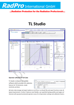
© Copyright 2026