
A New Method for General Solution Of System Of Higher
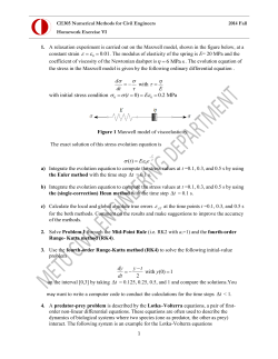
International Conference on Inter Disciplinary Research in Engineering and Technology [ICIDRET] 240 International Conference on Inter Disciplinary Research in Engineering and Technology [ICIDRET] ISBN Website Received Article ID 978-81-929742-5-5 www.icidret.in 14 - February - 2015 ICIDRET039 Vol eMail Accepted eAID I [email protected] 25 - March - 2015 ICIDRET.2015.039 A New Method for General Solution Of System Of Higher-Order Linear Differential Equations Srinivasarao Thota1, Shiv Datt Kumar2 Department of Mathematics, Motilal Nehru National Institute of Technology Allahabad Uttar Pradesh, India – 211004. Abstract- This paper presents a new method for solving system of higher-order linear differential equations (HLDEs) with constant coefficients; however the same idea can be extended to variable coefficients. Using the basic concept of inverse of matrix and variation of parameters, we develop a new method to solve system of HLDEs. Proposed method works for any right hand side function, so-called vector forcing function f (x) of given system of HLDEs. Selected examples are presented using proposed method to show the efficiency. Key words: Systems of higher-order linear differential equations, Variation of parameters, Inverse of matrix, General solution. I INTRODUCTION The systems of higher-order linear differential equations (HLDEs) have been vigorously pursued by many researchers and engineers and developed many different method to solve the system, for example, see [1-10]. Naturally, the systems of HLDEs arise in many applications of nuclear reactors, multi-body systems, vibrating wires in magnetic fields, models of electrical circuits, mechanical systems, robotic modeling, and diffusion processes etc. We consider the following type of systems of n linear differential equations of order m > 0, Am dm u ( x) dx m A1 d u ( x) A0u ( x) f ( x), dx (1) where, for i = 0, … , n, Ai are coefficient matrices of order n n , f ( x) ( f1 ( x), , f n ( x))T and u( x) (u1 ( x), , un ( x))T are an n-dimensional vector forcing function and unknown vector respectively. If the lading coefficient Am is non-singular, then the system of HLDEs (1) is called as of first kind, otherwise it is called second kind. In this paper, we present a new method to solve the system (1) of first kind with constant coefficients; however the same idea can be extended to variable coefficients. For obtaining the general solution of given system, we use the basic concepts of inverse of matrix and variation of parameters formula. Rest of the paper is organized as follows: In Section II, we present the proposed method to solve system of HLDEs and selected examples are presented in Section III to show the efficiency of proposed method. II A NEW METHOD FOR SYSTEM OF HIGHER-ORDER LINEAR DIFFERENTIAL EQUATIONS Recall the system of HLDEs given in Section I This paper is prepared exclusively for International Conference on Inter Disciplinary Research in Engineering and Technology [ICIDRET] which is published by ASDF International, Registered in London, United Kingdom. Permission to make digital or hard copies of part or all of this work for personal or classroom use is granted without fee provided that copies are not made or distributed for profit or commercial advantage, and that copies bear this notice and the full citation on the first page. Copyrights for third-party components of this work must be honoured. For all other uses, contact the owner/author(s). Copyright Holder can be reached at [email protected] for distribution. 2015 © Reserved by ASDF.international Cite this article as: Srinivasarao Thota , Shiv Datt Kumar. “A new method for general solution of system of higherorder linear differential equations.” International Conference on Inter Disciplinary Research in Engineering and Technology (2015): 240-243. Print. International Conference on Inter Disciplinary Research in Engineering and Technology [ICIDRET] L(u ( x)) Am dm u ( x) dx m A1 d u( x) A0u( x) f ( x), dx 241 (2) dm d A1 A0 , is n n matrix differential operator. Now the following theorem presents the algorithm to dx dx m compute the general solution of system (2), with given set of fundamental system of determinant of matrix differential operator L. where L Am Theorem 1: Given a fundamental system {v1 ( x), Am , vmn ( x)} , of T det( L) , then the system of higher-order LDEs dm u ( x) dx m A1 d u ( x) A0u ( x) f ( x), dx (3) has following solution mn det(W j ) f i ( x) n i 1 1 dx (1) det( Li ) v j ( x) det(W ) j 1 i 1 u ( x) n mn det(W j ) f i ( x) in n ( 1) det( L ) v ( x ) dx i j det( W ) i 1 j 1 where W is the Wronskian matrix of {v1 ( x), (4) , vmn ( x)} and Wi obtained from W by replacing the i-th column by mn-th unit vector; k i and det( L ) denotes the determinant of L after removing i-row and k-th column. Proof: Since the leading coefficient Am of system (3) is non-singular matrix, the inverse of L exists with det(L) = T as scalar differential operator of order mn. If {v1 ( x), , vmn ( x)} is fundamental system of T. Now the solution of system (3) can be obtained as u x Adj ( L) y( x) , where y( x) ( y1 ( x), , yn ( x))T is solution obtained from Tyi x fi x computed using the classical formulation variation of parameters as follows. The scalar differential equation Ty x f x can be reformulated as system of first order linear differential equation, say y '( x) My( x) f ( x) , where M is companion matrix. Now the solution of first order system is obtained as y( x) W W 1 f ( x) dx and the solution Ty x f x is the first row of y ( x) . The solution (4) satisfies given system of HLDEs, as follows: mn n det(W j ) f i ( x) i 1 1 dx (1) det( Li ) v j ( x) det( W ) i 1 j 1 L(u ( x)) L n mn det( W ) f ( x ) j i in n dx (1) det( Li ) v j ( x) det(W ) j 1 i 1 11 1 (1) det( L1 ) L (1) n 1 det( L1n ) ( f1 , , f n )T f det(W j ) f1 ( x) mn dx v j ( x) det(W ) ( 1) det( L ) j 1 nn n mn det(W j ) f n ( x) ( 1) det( Ln ) v ( x ) dx j det( W ) j 1 1 n n 1 Therefore, the solution (4) is general solution system (3). In following section, we present selected numerical examples (system of HLDEs with constant coefficients and variable coefficients) using proposed method presented in Theorem 1. Cite this article as: Srinivasarao Thota , Shiv Datt Kumar. “A new method for general solution of system of higherorder linear differential equations.” International Conference on Inter Disciplinary Research in Engineering and Technology (2015): 240-243. Print. International Conference on Inter Disciplinary Research in Engineering and Technology [ICIDRET] III 242 NUMERICAL EXAMPLES In this section, we present couple of examples for system of linear differential equations with constant coefficients (Example 1) and variable coefficients (Example 2) respectively, to show the efficiency of proposed method in Theorem 1. Example 1: Consider the following system of linear differential equations of order two with constant coefficients d2 u1 ( x) u1 ( x) 2u2 ( x) sin( x), dx 2 d2 d u ( x) u2 ( x) e 3 x . 2 2 dx dx The system (5) can be written in matrix notations as L(u( x)) f ( x), with L A2 (5) d2 d A1 A0 , where 2 dx dx sin( x) 1 0 0 0 1 2 u1 ( x) A2 , f ( x) 3 x . , A1 , A0 and u ( x) 0 1 0 1 0 0 u2 ( x ) e If we denote D D2 1 2 d , then L . Following procedure in Theorem 1, we have 2 dx D D 0 Ty( x) D4 y( x) D3 y( x) D2 y( x) Dy( x) f ( x) , here y( x) ( y1 ( x), y2 ( x))T . Now from Theorem 1, we have the general solution of given system (5) as follows x 1 c1 cos( x) c2 sin( x) cos( x) 2c3 c4 e x e 3 x u ( x ) 1 2 60 , u ( x) 1 3 x x u2 ( x ) c3 c4 e e 12 where c1,c2,c3 and c4 are arbitrary constants. Example 2: Consider the following system of linear differential equations of order one with variable coefficients d d u1 ( x) x u2 ( x) u1 ( x) (1 x)u2 0, dx dx d u2 ( x ) u2 ( x ) e 2 x . dx The matrix representation of system (5) is L(u ( x)) A1 (6) d u ( x) A0u ( x) f ( x) , where dx 0 1 x 1 1 x u1 ( x) A1 , f ( x) 2 x . , A0 and u ( x) 0 1 0 1 u ( x ) 2 e D 1 Matrix differential operator L 0 given system (6) as follows xD 1 x d . Following Theorem 1, we have the general solution of , where D D 1 dx Cite this article as: Srinivasarao Thota , Shiv Datt Kumar. “A new method for general solution of system of higherorder linear differential equations.” International Conference on Inter Disciplinary Research in Engineering and Technology (2015): 240-243. Print. International Conference on Inter Disciplinary Research in Engineering and Technology [ICIDRET] 243 x 1 x c e 2c2 xe x c2 e x e 2 x e 2 x u1 ( x) 1 3 9 , u ( x) 1 2x x u2 ( x ) c e e 2 3 where c1 and c2 are arbitrary constants. IV CONCLUSION In this paper, we have presented a new method for solving system of higher order linear differential equations. This proposed method works for any vector forcing function of given system of HLDEs. The proposed method is developed using the basic concept of inverse of matrix and variation of parameters. Couple of examples (systems with constants coefficients and variable coefficients) are presented using proposed method to show the efficiency. REFERENCES [1] D. Sengupta: Resolution of the identity of the operator associated with a system of second order differential equations, J. Math. Comput. Sci. 5, No. 1, 56-71, 2015. [2] D. Sengupta: On the expansion problem of a function associated with a system of second order differential equations, J. Math. Comput. Sci. 3, No. 6, 1565-1585, 2013. [3] D. Sengupta: Asymptotic expressions for the eigenvalues and eigenvectors of a system of second order differential equations with a turning point (Extension II), International Journal of Pure and Applied Mathematics, Volume 78 No. 1, 85-95, 2012. [4] S. Suksern, S. Moyo, S.V. Meleshko: Application of group analysis to classification of systems of three second-order ordinary differential equations, John Wiley \& Sons, Ltd. DOI: 10.1002/mma.3430, 2015. [5] Vakulenko, S., Grigoriev, D. and Weber, A.: Reduction methods and chaos for quadratic systems of differential equations. Studies in Applied Mathematics, doi: 10.1111/sapm. 12083, 2015. [6] Mukesh Grover: A New Technique to Solve Higher Order Ordinary Differential equations. IJCA Proceedings on National Workshop-Cum-Conference on Recent Trends in Mathematics and Computing 2011 RTMC, May 2012. [7] R. Ben Taher and M. Rachidi: Linear matrix differential equations of higher-order and applications. Electronic Journal of Differential Equations, 2008(95), 1-12, 2008. [8] G. I. Kalogeropoulos, A. D. Karageorgos, and A. A. Pantelous: Higher-order linear matrix descriptor differential equations of Apostol-Kolodner type. Electronic Journal of Differential Equations, 2009(25), 1-13, 2009. [9] S. Abramov: EG - eliminations. Journal of Difference Equations and Applications, 5, 393-433, 1999. [10] Carole EL BACHA: Methodes Algebriques pour la Resolution dEquations Differentielles Matricicelles d'Ordre Arbitraire. PhD thesis, LMC-IMAG, 2011. [11] E. A. Coddington and R. Carlson: Linear ordinary differential equations. Society for Industrial and Applied Mathematics (SIAM), 1997. [12] Apostol, Tom M.: Calculus, volume II. John Wiley \& Sons (Asia) Pte. Ltd., New York-Chichester-Brisbane-TorontoSingapore (2002). [13] Henry J. Ricardo: A Modern Introduction to Differential Equations, Second Edition, Academic Press, March, (2009). Cite this article as: Srinivasarao Thota , Shiv Datt Kumar. “A new method for general solution of system of higherorder linear differential equations.” International Conference on Inter Disciplinary Research in Engineering and Technology (2015): 240-243. Print.


© Copyright 2026