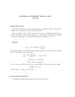
SPECIAL FEATURE
Fossils, phylogenies, and the challenge of
preserving evolutionary history in the face of
anthropogenic extinctions
Danwei Huanga,b, Emma E. Goldbergc, and Kaustuv Royd,1
a
Department of Biological Sciences, National University of Singapore, Singapore 117543, Singapore; bDepartment of Earth and Environmental Sciences,
University of Iowa, Iowa City, IA 52242; cDepartment of Ecology, Evolution and Behavior, University of Minnesota, St Paul, MN 55108; and dSection of Ecology,
Behavior and Evolution, University of California, San Diego, La Jolla, CA 92093
extinction
| phylogenetic diversity | phylogeny | fossil record | bivalves
E
xtinction of any species or higher taxon invariably results in
some loss of existing evolutionary history (EH), but a major
concern about extinctions driven by anthropogenic impacts is
that they may remove a disproportionately large amount of such
history (1–3). In groups as varied as birds, mammals, and plants,
studies have shown that extinctions of species currently on the
International Union for the Conservation of Nature Red List of
Threatened Species would lead to a much larger loss of EH than
expected under randomly distributed extinction of the same
number of species (4–6). This disproportionate loss of EH stems
from phylogenetic clustering of anthropogenic extinctions (1) with
a bias toward the loss of species-poor and geologically old taxa (7–9).
Such predictions, along with the realization that not all species
currently threatened by human activities can be saved, have
motivated the development of various strategies for minimizing
the loss of EH (8, 10, 11). These approaches primarily target
lineages that are old but species poor in an attempt to protect large
amounts of EH and, presumably, also unique traits and functions
that may affect future evolutionary potential (10, 12).
Although the disproportionate loss of EH caused by anthropogenic extinctions is increasingly evident, surprisingly little is
known about the loss of EH during extinctions in the geological
past. The rich archive of extinctions preserved in the fossil record
has been the main source of insights about the nature of the
extinction process (13–15), and it provides the baseline against
which the magnitude of the current crisis has been measured
www.pnas.org/cgi/doi/10.1073/pnas.1409886112
(16). Comparisons of ecological and biogeographic components
of past and present extinctions also hold great potential for
predicting the nature of future losses (17, 18). Although paleontological studies have tested for age-related bias in extinction
vulnerability (19–22), such analyses have focused primarily on
background extinctions rather than on selectivity across major
extinction events (23). However, without a better understanding
of patterns of loss of EH during major pulsed extinctions in the
geological past, we cannot answer the fundamental question of
whether we, as a species, are pruning the tree of life in a unique
manner. Such an understanding requires developing a comparative framework that includes both paleontological and
neontological data.
A major impediment to comparing anthropogenic impacts on
EH with those during past extinctions is that the methods used in
each case differ. Analyses of future losses caused by anthropogenic extinctions primarily have used tree-based measures of EH
(24, but see ref. 25) that are not easily applicable to extinct taxa
for which large phylogenies are still lacking. More importantly,
even when phylogenies of extinct taxa are available, the differences in the nature of paleontological and molecular phylogenies
complicate direct comparisons. In paleontological phylogenies, a
species maintains its identity over time as long as its traits remain
relatively constant. This property allows “budding cladogenesis”
in which a parent species remains unaffected while giving rise to
a daughter (Fig. 1) (26, 27). In contrast, molecular (or cladistic)
phylogenies allow only “bifurcating cladogenesis” in which the
parent lineage is replaced by two daughters (or more daughters
Significance
Anthropogenic impacts are endangering many species, potentially leading to a disproportionate loss of evolutionary history
(EH) in the future. However, surprisingly little is known about
the loss of EH during extinctions in the geological past, and
thus we do not know whether anthropogenic extinctions are
pruning the tree of life in a manner that is unique in Earth’s
history. Comparisons of EH loss during past and ongoing
extinctions is difficult because of conceptual differences in how
ages are estimated from paleontological data versus molecular
phylogenies. We used simulations and empirical analyses to
show that the differences between the two data types do not
preclude such comparisons, which are essential for improving
evolutionarily informed models of conservation prioritization.
Author contributions: D.H., E.E.G., and K.R. designed research, performed research, analyzed data, and wrote the paper.
The authors declare no conflict of interest.
This article is a PNAS Direct Submission.
Data deposition: All datasets and R scripts are available at dx.doi.org/10.5281/zenodo.
11404.
1
To whom correspondence should be addressed. Email: [email protected].
This article contains supporting information online at www.pnas.org/lookup/suppl/doi:10.
1073/pnas.1409886112/-/DCSupplemental.
PNAS | April 21, 2015 | vol. 112 | no. 16 | 4909–4914
EARTH, ATMOSPHERIC,
AND PLANETARY SCIENCES
Anthropogenic impacts are endangering many long-lived species
and lineages, possibly leading to a disproportionate loss of existing
evolutionary history (EH) in the future. However, surprisingly little is
known about the loss of EH during major extinctions in the geological
past, and thus we do not know whether human impacts are pruning
the tree of life in a manner that is unique in the history of life. A major
impediment to comparing the loss of EH during past and current
extinctions is the conceptual difference in how ages are estimated
from paleontological data versus molecular phylogenies. In the
former case the age of a taxon is its entire stratigraphic range,
regardless of how many daughter taxa it may have produced; for
the latter it is the time to the most recent common ancestor shared
with another extant taxon. To explore this issue, we use simulations to understand how the loss of EH is manifested in the two
data types. We also present empirical analyses of the marine
bivalve clade Pectinidae (scallops) during a major Plio–Pleistocene
extinction in California that involved a preferential loss of younger
species. Overall, our results show that the conceptual difference in
how ages are estimated from the stratigraphic record versus molecular phylogenies does not preclude comparisons of age selectivities of past and present extinctions. Such comparisons not only
provide fundamental insights into the nature of the extinction
process but should also help improve evolutionarily informed
models of conservation prioritization.
EVOLUTION
Edited by David Jablonski, The University of Chicago, Chicago, IL, and approved January 1, 2015 (received for review May 27, 2014)
extinction biased to old A B C D E F G H I
absolute age (A, I) 8 1 3 4 2 1 3 1 6
A B C D E F G H I
1 1 3 2 1 1 2 2 7
extinction biased to young
absolute age (F, H)
Full, budding branching history
A B C
t=0
D E F G
J
H
I
K
MN
L
Stratigraphic ranges
A B C D E F G H I
8 1 3 4 2 1 3 1 6
t=4
Bifurcating phylogeny
A B C D E F G H I
1 1 3 2 1 1 2 2 7
t=8
extinction biased to old
relative age (C, I)
extinction biased to young
relative age (A, B)
Fig. 1. A simple tree showing how the full branching history of a clade can
be reduced to either stratigraphic ranges or a bifurcating phylogeny. A clade
undergoes speciation (assumed here to be budding, with survival of the
parent) and extinction, with nine lineages (A–I) surviving to the focal time
(t = 0). The stratigraphic range and absolute age of each surviving species are
determined by the time of its first appearance in the fossil record, without
reference to species relationships. The bifurcating phylogeny is determined by
the divergence times of surviving species relative to one another, without
regard for their original times of speciation. Colors illustrate the four scenarios
of age-dependent extinction at the focal time. Note that the oldest species
differ—in both identity and age—between the absolute and relative age
definitions, as do the youngest species. Thus, stratigraphic and phylogenetic
diversity are differently affected by the loss of species.
in the case of multifurcation), even for speciation events that were,
in fact, budding (Fig. 1) (26). Thus, the discrepancy between the
stratigraphic and cladistic representations depends on the frequency of budding versus bifurcating speciation, which remains
unknown at present despite well-documented cases of budding
cladogenesis in the fossil record (26–28).
Whether cladogenesis is viewed as budding or bifurcating has
important consequences for assessing what the “age” of a species
is and consequently for analyses of age selectivities as well as other
aspects of evolutionary dynamics (29). For budding cladogenesis,
the age of a taxon is its entire stratigraphic range (hereafter
absolute age) regardless of daughter taxa it may have produced,
whereas for bifurcating cladogenesis the age of the taxon is the
time to the most recent common ancestor shared with another
extant taxon (hereafter relative age) (Fig. 1) (26, 29). Comparing
paleontological insights about evolutionary dynamics with those
inferred from molecular phylogenies requires us to understand
better the consequences of this difference for empirical analyses.
For the question addressed here, the age definition used will affect
empirical tests of age selectivity during extinctions. It also will
affect simulation tests, such as when choosing taxa for removal
during an age-biased extinction event (Fig. 1). We emphasize,
however, that these two age definitions are simply different
conceptualizations of a given biological history. Extinction selectivity is expected to be based on traits (e.g., geographic range,
body size) rather than on age per se, so any signal of age-dependent
extinction more likely reflects its relationship to other traits.
Our goal here is to understand how the loss of EH is manifested in budding versus bifurcating phylogenies. We start with
simulations to illustrate how a given extinction event erodes EH
on each of these types of phylogenies. We then explore this issue
empirically using a phylogeny of living and extinct marine scallops (Pectinidae) that experienced elevated extinction during the
Plio–Pleistocene transition (30).
Measuring the Loss of Evolutionary History
Although many metrics are available to quantify loss of EH (12,
31), the one most commonly used to estimate potential losses of
EH caused by anthropogenic extinctions is phylogenetic diversity
(PD), defined as the sum of branch lengths on a phylogenetic
4910 | www.pnas.org/cgi/doi/10.1073/pnas.1409886112
tree (24). Because of its widespread application (1, 4, 32–34), we
focus on PD here.
As discussed above, although reconstructed bifurcating phylogenies estimate the relative divergence time of two lineages,
stratigraphic range data approximate the absolute duration of
each taxon (35) independent of other taxa derived from it. When
branches are pruned off a clade, the loss of EH may look quite
different from a paleontological perspective (Fig. 1). We define
stratigraphic diversity (SD), analogously to PD, as the sum of the
stratigraphic ranges of taxa within a clade. Loss of PD and SD
may scale differently with extinction intensity and selectivity in
the two types of trees (Fig. 1).
One window into how extinction erodes EH comes from its
age selectivity. Paleontological studies have long tested for age
bias in extinctions, starting with the work of Simpson (36) and the
much-cited conclusion of Van Valen (19) that the extinction risk
of a taxon is independent of its age. Subsequent studies at different taxonomic levels and across various extinction intensities
instead have found evidence for preferential extinctions of either
older (21) or younger taxa (20). However, virtually all these
analyses focused on background rather than on pulsed extinctions.
For anthropogenic extinctions, disproportionately large losses of
PD predicted for many groups (4–6, 9) suggest the preferential
endangerment of older and species-poor lineages, although a
recent study of mammals failed to find such age bias (37).
Simulations
Loss of EH. We designed a set of simulations to compare the loss
of EH under the same extinction event using paleontological and
molecular phylogenies, considering different effects of species
ages on extinction risk. Our central question is whether excessive
loss of older (or younger) taxa as measured on one phylogeny type
is detectable using the other.
We simulated phylogenies under a constant-rates birth–death
process with budding speciation, retaining only species that survived to the time of observation. By assuming that all speciation
events are budding, we maximize the difference between absolute
and relative ages and hence the discrepancy between SD and PD.
Our analyses are based on these histories and do not incorporate
uncertainty in estimating phylogeny or stratigraphic range. Two
alternative simulation programs were used, SimTreeSDD (Figs. 2
and 3) (38) and paleotree (39) (Figs. S1–S3 and SI Materials and
Methods). We then reduced the outcome of the branching process
to either stratigraphic ranges, which define the “absolute age” of
each species, or to a bifurcating phylogeny on which the terminal
branch length is the “relative age” of each species (Fig. 1 and SI
Materials and Methods).
Trees were simulated for two pairs of speciation and extinction
rates, capturing relatively low and high extinction [« = μ/λ = 0.2
or 0.8, where λ is the origination rate and μ the extinction rate
(40)] while holding the net diversification rate (r = λ − μ) constant.
We subjected each simulated tree to five different forms of age
bias in extinction risk (Fig. 1 and SI Materials and Methods): extinction risk independent of both absolute age and relative age, extinction risk increasing linearly with absolute or relative age, or
extinction risk decreasing linearly with absolute or relative age.
We considered four different extinction intensities (m) for each
age structure of extinction, removing between 10% and 80% of
species. Note the distinction between the background extinction
rate of the clade (μ, used to simulate the trees) and the intensity
of the specific extinction event (m). We are interested in age bias
associated with the latter.
For each simulation outcome, we computed the loss of EH
measured by PD (24) as the sum of all of the branch lengths
(terminal and internal) removed from the phylogeny. We also
computed the corresponding loss of EH measured by the paleontological metric SD, the loss of which is defined here as the
sum of all absolute ages removed. Letting the subscript “observed” denote EH remaining after the extinction event in any
particular outcome and “random” denote EH remaining when
age does not influence extinction risk, we quantify the excess loss
Huang et al.
C
D
Fig. 2. PDexcess based on bifurcating phylogenies versus the corresponding
SDexcess for the same extinction event under four age-biased extinction
regimes. Individual colors depict extinction probability increasing linearly
with absolute age (stratigraphic range) or with relative age (phylogenetic tip
length) or decreasing linearly with absolute age or with relative age. Excessover-random losses (see main text) are shown for four extinction intensities
(m = 10, 30, 50, or 80%) and trees simulated with two pairs of speciation (λ)
and extinction (μ) rates (e = μ/λ = 0.2 or 0.8). (A) One thousand trees with e =
0.8. (B) Largest quartile of trees (250) with e = 0.8. (C) One thousand trees
with e = 0.2. (D) Largest quartile of trees (250) with e = 0.2.
of EH with EHexcess = (EHrandom − EHobserved)/EHrandom (41),
where EH may be either PD or SD. This excess quantity is
positive when more EH is lost than expected by chance and
negative when less EH is lost.
When loss of species during an extinction event is independent
of both absolute and relative age, we find that SD loss is greater
than PD loss (Fig. S1). This effect is driven by the extinction of
older species. When species of large absolute age go extinct, they
take their entire EH with them, whereas when species of large
relative age go extinct, part of their shared history (internal
branches) may remain on the phylogeny (e.g., species A in Fig. 1).
When an extinction event preferentially removes taxa with
older absolute ages, SDexcess values are strongly positive because
less SD remains than under random extinction, but PDexcess
values are smaller or even negative (Fig. 2, blue). The discordance between SDexcess and PDexcess decreases with increasing
tree size and extinction intensity. When extinction most affects
taxa with older relative ages, both SDexcess and PDexcess are
generally positive (Fig. 2, red). These results together show that
when an extinction event preferentially affects older species—by
either definition—paleontological studies are more likely to
detect the effect than are neontological studies.
When extinction preferentially removes species of younger
absolute or relative age, both SDexcess and PDexcess values are
often negative although many are near zero (Fig. 2, green and
purple). We see the largest effect of young-biased extinction and
the greatest consequent loss of EH when μ is low but m is high.
These age-biased extinction results are determined by three
factors. First, SD loss is generally greater than PD loss under any
extinction regime, as discussed above (Fig. S1). Second, the age
distribution of an exponentially growing clade is dominated by
the continual production of younger species (42). Thus, even
when risk during an extinction event is independent of age, more
extinctions are of younger species simply because younger species
are more numerous. This inherent feature of random extinction
overshadows much of the signal of young-biased extinction while
Huang et al.
Taxon Age Selectivity. We used the same simulations to test whether
age bias during extinction events is manifested statistically in phylogenetic and stratigraphic data. Following Finnegan et al. (20), we
used a binomial logistic regression model to test for the effect of age
on the survival of a species. The odds ratio of a logistic regression
conveniently summarizes the results: the log-odds are expected to
be negative when extinction preferentially removes older taxa and
positive when younger taxa suffer greater extinction. Our central
question is again whether an extinction event biased by absolute
age can be recognized by studies using relative age, and similarly
whether absolute age studies can detect relative age-biased
extinction.
When extinction risk is independent of age, no statistically significant age bias is detected for either definition of age (Fig. 3 I
and J). We do see a slight influence of extinction intensity (m) on
effect size, however, with positive log-odds (in the direction of
young-biased extinction) for low m and negative log-odds for high
m. We attribute this difference to the age distributions, discussed
above. With an overrepresentation of young species, especially as
measured by relative age, old species are less likely to be captured
in any one extinction episode.
When extinction risk is biased to older absolute or relative age,
log-odds almost always are negative. If absolute age drives the
risk (Fig. 3 A and B), the signal is strongest when measured by
absolute age, as expected, but also generally is significant when
A
B
C
D
E
F
G
H
I
J
Fig. 3. Taxon age selectivity under four age-biased extinction regimes plus
a null model of random, age-independent extinction. (A–J) Bars represent
the natural logarithm of the odds ratio (log-odds) based on a binomial
logistic regression model. Log-odds are expected to be negative when extinction preferentially removes older taxa and positive when younger taxa
are more likely to go extinct. Solid colors represent log-odds calculated based
on absolute ages from stratigraphic ranges; shaded colors represent log-odds
calculated using relative ages from bifurcating phylogenies. Shown are logodds under four extinction intensities (m = 10, 30, 50, or 80%) for trees simulated with two pairs of speciation (λ) and extinction (μ) rates (e = μ/λ = 0.2 or
0.8). Numbers above or below bars represent the proportions of trees that
show a statistically significant effect of age on species survivorship.
PNAS | April 21, 2015 | vol. 112 | no. 16 | 4911
SPECIAL FEATURE
EVOLUTION
B
highlighting the signal of old-biased extinction. Third, the frequencies of absolute and relative ages within a clade differ. Because
the birth of a new species reduces the relative but not absolute age
of the parent lineage, the relative age distribution is even more
strongly biased toward the young. Consequently, there is less scope
for extinctions biased by relative age, reducing the size of PDexcess
relative to SDexcess.
EARTH, ATMOSPHERIC,
AND PLANETARY SCIENCES
A
measured by relative age except for low extinction intensity. If
relative age drives the risk (Fig. 3 C and D), the age bias of
extinction is detected less reliably when measured by absolute
age. We ascribe this difference to the smaller pool of species of
old relative age, compared with the absolute age distribution. As
in the previous case, the results for the two types of age match
best when both m and « are high, and the mismatch is worst for
very low extinction intensities, especially when « is low (Fig. 3).
In cases where we preferentially remove younger taxa, using
either relative or absolute ages, the log-odds are always positive,
as expected (Fig. 3 E–H). The effect size is larger for absolute
age when extinction risk is based on absolute age, and likewise
for relative age. The results rarely are statistically significant,
however. We again attribute this difference in effect size to the
overrepresentation of young species in a clade: young-biased extinction then has less effect on the age distributions of victims
and survivors.
4912 | www.pnas.org/cgi/doi/10.1073/pnas.1409886112
Holocene
Pleistocene
Miocene
Pliocene
5.332
2.588
0.0117
Oligocene
23.03
33.9
Eocene
Paleocene
56
66
Late
Cretaceous
100.5
Early
Cretaceous
145
Plio–Pleistocene Extinctions
Paleontological analyses of age-related bias in extinction vulnerability (19–22) have focused on background extinctions rather than
on selectivity across major extinction events (23), whereas analyses
of anthropogenic extinctions are focused on a single, unfolding
event. As a first step toward reducing this information gap, we
tested for age-related bias in the Plio–Pleistocene extinction of
marine scallops (family Pectinidae) in California.
The Late Cenozoic fossil record of California preserves a rich
assemblage of shallow marine molluscan species, which suffered
a major extinction during the Plio-Pleistocene transition (30),
a time of elevated extinctions of mollusks in other regions of the
world as well (43–45). The bivalve family Pectinidae suffered
particularly heavy losses in California during this extinction event
with little subsequent evolutionary rebound (46). The systematics
of the Neogene pectinids of California also is well studied,
making this an ideal group for phylogenetic analyses of extinction selectivity (47–49). To perform these extinction analyses, we
used Bayesian methods to infer a time-calibrated phylogeny of
living and Neogene pectinid species based on molecular and
fossil data, generating a posterior set of 1,000 fully resolved trees
(SI Materials and Methods). Of the 50 species of Plio–Pleistocene
scallops known from California, 25 were lost during this extinction
event (Fig. 4). Despite this 50% reduction in species richness, the
loss of PD in this case was significantly less than expected across
the 1,000 posterior trees (Fig. S4), suggesting a preferential loss of
younger species during this extinction. Comparisons of relative
ages produce a qualitatively similar result, with the age selectivity
log-odds being larger than under age-independent extinctions,
although this finding is not significant across all trees (Fig. S5).
The loss of SD using absolute ages shows that SDexcess is negative, but the confidence interval (CI) is broad and overlaps with
zero (mean SDexcess = −0.11, 95% CI = −0.38 to 0.08 based on
1,000 iterations). The log-odds using absolute ages are also
positive (0.02), but, again, are not significant (P = 0.75). Taken
together, although all metrics indicate a preferential loss of
younger scallop species during this extinction event, only PD loss
using relative ages shows a significant signal.
We also tested for selectivity in absolute ages of other bivalve
species during the Plio–Pleistocene extinction using stratigraphic
ranges from Hall (30) because a phylogeny for nonpectinid species
involved in this event is not currently available. In contrast to the
scallops, species across all families of bivalves show an overall
negative log-odds (−0.03, n = 286), as do Veneridae, the most
species-rich family in this fauna (−0.05, n = 33), but neither effect
is significant (P = 0.16 overall and P = 0.52 for Veneridae). Thus,
the bias toward a loss of younger species seen in the pectinids is
not reflected in other families, suggesting that clades can differ in
their patterns of species age selectivity during the same extinction event.
Euvola vogdesi
Euvola coalingaensis
Euvola heimi
Euvola juanensis
Euvola refugioensis
Euvola keepi
Euvola lecontei
Euvola hartmanni
Euvola diegensis
Euvola carrizoensis
Euvola bellus
Euvola aletes
Leopecten stearnsii
Amussiopecten venvlecki
Amusium lompocensis
Lyropecten terminus
Lyropecten miguelensis
Lyropecten estrellanus
Lyropecten pretiosus
Lyropecten modulatus
Lyropecten crassicardo
Lyropecten gallegosi
Lyropecten cerrosensis
Lyropecten catalinae
Lyropecten vaughni
Lyropecten tiburionensis
Nodipecten veatchii
Nodipecten subnodosus
Nodipecten arthriticus
Argopecten ventricosus
Argopecten purpuratus
Argopecten sverdrupi
Argopecten subdolus
Argopecten percarus
Argopecten mendenhalli
Argopecten invalidus
Argopecten hakei
Argopecten ericellus
Argopecten deserti
Argopecten cristobalensis
Argopecten callidus
Argopecten abieties
Leptopecten weaveri
Leptopecten tumbezensis
Leptopecten tolmani
Leptopecten praevalidus
Leptopecten pabloensis
Leptopecten latiauratus
Leptopecten discus
Leptopecten bilineatus
Leptopecten andersoni
Paraleptopecten bellilamellatus
Chlamys rubida
Chlamys islandica
Chlamys hastata
Chlamys sespeensis
Chlamys sanctiludovici
Chlamys opuntia
Chlamys jordani
Chlamys hodgei
Chlamys hertleini
Chlamys egregius
Chlamys corteziana
Chlamys branneri
Chlamys bartschi
Patinopecten propatulus
Patinopecten oregonensis
Patinopecten lohri
Patinopecten healeyi
Patinopecten haywardensis
Patinopecten caurinus
Yabepecten condoni
Swiftopecten parmeleei
Swiftopecten nutteri
Vertipecten perrini
Vertipecten kemensis
Vertipecten fucanus
Vertipecten bowersi
Lituyapecten turneri
Lituyapecten purisimaensis
Lituyapecten falorensis
Lituyapecten dilleri
Crassadoma gigantea
Crassadoma benedicti
Spathochlamys vestalis
Delectopecten vancouverensis
Delectopecten pedroanus
Delectopecten peckhami
Delectopecten harfordus
Extant today
Extinct after 2.5 mya
Extinct at 2.5 mya
Extinct before 2.5 mya
Fig. 4. Stratigraphic ranges (thick lines) and phylogenetic relationships (thin
lines) of 89 Late Oligocene to Recent species of scallops (Pectinidae) known
from California. The tree shown forms the backbone for generating 1,000 fully
resolved Bayesian posterior trees used to analyze extinctions occurring at the
Plio–Pleistocene transition, ∼2.5 Mya, which removed 25 of the 50 species
present at that time. Species names and stratigraphic ranges are colored
according to times of extinction relative to the Plio–Pleistocene transition.
Discussion
Comparing the loss of EH during major extinction events using
paleontological versus molecular phylogenies can be difficult
because of the conceptual difference in how ages are estimated. However, our simulations and empirical analyses show
that estimated EH losses during major extinction events tend
to be qualitatively similar despite this difference. The simulations
also show that extinction generally removes EH more rapidly in
paleontological data than in molecular phylogenies, where the
loss is buffered by shared history. Preferential extinction of older
taxa leads to large losses of EH in both cases, but the magnitudes
differ among the two data types with molecular phylogenies
again providing the more conservative estimates. This asymmetry
when comparing phylogeny-based EH losses with those from the
fossil record indicates that analyses of major extinction events in
the geologic past can provide a meaningful baseline for comparing patterns of endangerment in ongoing extinctions. The
absence of excess loss of EH observed during past extinction
events would indicate that there is little natural analog for the
preferential endangerment of older lineages currently seen from
anthropogenic impacts. Furthermore, our results suggest that
such comparisons can be based on either the sum of the ages or
the age distributions themselves, although conceptually the latter
may be preferable.
When extinctions preferentially remove younger species, the
signal is muted in paleontological data and more so in phylogenies. We ascribe this lower power to the age distributions of
species at any point in time being skewed toward the younger
ages. Therefore, these results caution that type II errors are most
likely to arise when a bias toward younger ages in species-level
extinctions is suspected. Such a bias should be easier to detect at
Huang et al.
1. Purvis A, Agapow P-M, Gittleman JL, Mace GM (2000) Nonrandom extinction and the
loss of evolutionary history. Science 288(5464):328–330.
2. von Euler F; Euler von F (2001) Selective extinction and rapid loss of evolutionary
history in the bird fauna. Proc Biol Sci 268(1463):127–130.
3. Sechrest W, et al. (2002) Hotspots and the conservation of evolutionary history. Proc
Natl Acad Sci USA 99(4):2067–2071.
4. Mooers AØ, Atkins RA (2003) Indonesia’s threatened birds: Over 500 million years of
evolutionary heritage at risk. Anim Conserv 6(2):183–188.
Huang et al.
Conclusions
Although there is little doubt that anthropogenic impacts are endangering many long-lived species and lineages, potentially leading to their extinction and thus a disproportionate loss of existing
EH, whether this bias is likely to be a unique evolutionary legacy
of our species remains unknown. The rich archive of past extinctions preserved in the fossil record holds the key to answering this
question, and our results show that the conceptual difference in
how ages are estimated from the stratigraphic record versus phylogenies does not preclude comparisons of age selectivities of past
and present extinctions. Such comparisons can provide fundamental understanding about the nature of the extinction process
and also can help us develop more evolutionarily informed models
of conservation prioritization.
Materials and Methods
Further details about simulations, data, and analytical methods are provided
in SI Materials and Methods.
ACKNOWLEDGMENTS. We thank David Jablonski and Neil Shubin for the
invitation to write this paper, and David Jablonski and two anonymous
reviewers for very helpful comments on previous versions of the manuscript.
D.H. thanks Gregory Rouse for providing laboratory and computational support.
5. Davies TJ, et al. (2008) Colloquium paper: Phylogenetic trees and the future of
mammalian biodiversity. Proc Natl Acad Sci USA 105(Suppl 1):11556–11563.
6. Vamosi JC, Wilson JRU (2008) Nonrandom extinction leads to elevated loss of angiosperm evolutionary history. Ecol Lett 11(10):1047–1053.
7. Mace GM, Gittleman JL, Purvis A (2003) Preserving the tree of life. Science 300(5626):
1707–1709.
8. Isaac NJB, Turvey ST, Collen B, Waterman C, Baillie JEM (2007) Mammals on the EDGE:
Conservation priorities based on threat and phylogeny. PLoS ONE 2(3):e296.
PNAS | April 21, 2015 | vol. 112 | no. 16 | 4913
SPECIAL FEATURE
EVOLUTION
addition, paleontological data show that many geologically old
lineages tend to be morphologically unremarkable (66). Finally,
some species-poor, long-lived lineages are likely to fit the “dead
clade walking” model of Jablonski (67, 68), in which formerly
diverse groups are bottlenecked by an extinction event without
subsequent recovery. These patterns suggest that we need to
better understand how age-biased extinctions, especially those that
preferentially remove older taxa, affect future evolutionary trajectories. Given the problems of estimating extinction rates from
molecular phylogenies of extant species (69, 70) and the uncertainties associated with ancestral state reconstructions (71), data
from the fossil record are critical for addressing this issue. However, although much of our insight into the extinction process
comes from paleontological studies, the issues of age bias and
trait loss during major extinction events and their effects on
subsequent recoveries still remain poorly explored.
Our finding that the signal of preferential extinctions of young
species can be hard to detect through the approaches commonly
used to study age-biased extinctions also has important implications. As discussed above, evolutionary conservation studies
have focused on the endangerment of older lineages, but many
young species can have unique traits and important functional
and ecological roles. Adaptive radiations, in particular, often
contain many unique young species, and examples abound of
such species being negatively affected by anthropogenic impacts
(e.g., refs 72–75). A focus on the loss of EH alone is likely to
underestimate the erosion of trait and functional diversity
resulting from such extinctions in young radiations, especially for
smaller clades. Such losses of young species also would suggest
that anthropogenic impacts have the potential to suppress origination rates in some clades, although the effect remains to be
quantified. The same lack of power also can plague analyses of
past extinctions of species, as seen for the pectinids here. Thus,
although a bias toward younger genera of marine invertebrates
during background extinction has been documented, establishing
whether a similar bias exists for species, especially during major
extinctions, may require alternative analytical approaches.
EARTH, ATMOSPHERIC,
AND PLANETARY SCIENCES
higher taxonomic levels where the age distributions contain a
larger proportion of older taxa. Available empirical evidence is
generally consistent with this view, with at least one previous study
finding a significant bias toward younger genera during background extinctions (20). Our empirical results show that species
loss of pectinids during a major extinction event in California involved preferential loss of younger taxa; however, the effect is
significant only using PD, indicating that the age bias in this case is
more closely tied to relative than to absolute age. Because these
extinct species had geographic ranges significantly smaller than
those of the survivors (50), we hypothesize that the ranges of
parent species were reduced by giving rise to daughters; speciation
made the parent taxa younger and range-restricted (e.g., refs. 51
and 52), and thus more extinction prone.
In addressing our central question of whether we are currently
trimming the tree of life in a manner different from in the past,
our results are encouraging in that they identify ways of making
comparisons across extinction events using paleontological data
and molecular phylogenies. As discussed above, virtually all paleontological analyses of the age selectivity of extinctions have
focused on background extinctions, integrating over a substantial
history of individual clades (20, 21, 23), but the best analogs of
the current extinction crisis are the more severe extinction pulses
of the past, either regional or global (16). Furthermore, the incomplete nature of the fossil record and the difficulties involved
in identifying fossil species have led previous analyses to focus on
higher taxa rather than species (but see ref. 21). Because the age
distributions of higher taxa are different from those of species, it
is difficult to compare patterns of age selectivity across taxonomic levels. Thus, existing studies do not readily allow direct
comparisons of past losses of EH with those predicted for anthropogenic extinctions. Although temporal durations of species
in the fossil record are more difficult to estimate reliably than
those of higher taxa (23), a number of paleontological studies
have used fossil species successfully to test important evolutionary
and biogeographic hypotheses (21, 51–56) as well as various
aspects of the extinction process (57–59). With the increasing
availability of large, taxonomically standardized paleontological
databases, analyses of age selectivity of extinctions at the species
level, such as the one undertaken here, are now feasible, especially on regional scales. In addition, molecular sequence data
for living species continue to accumulate in GenBank and other
repositories, and novel approaches for integrating fossil species
into molecular phylogenies are now available (60, 61), making it
feasible to undertake age-selectivity analyses of past and present
extinctions using a common currency of relative ages estimated
from phylogenies.
Although much remains to be learned about how extinctions,
past and present, remove EH, the long-term evolutionary consequences of age-biased extinctions are even less understood. The
use of PD in conservation is based primarily on a proposed correlation between PD and trait diversity (24, 62, 63). Under this
model, excessive loss of PD would result in a disproportionate
loss of traits and consequently in a greater effect on future evolutionary trajectories. Species in geologically old and species-poor
lineages are considered to be particularly important from this
perspective because they alone represent millions of years of trait
evolution, and considerable effort is being put into identifying
such taxa, generally known as “Evolutionarily Distinct and Globally Endangered” (EDGE) species (8, 11, 64). However, empirical
analyses using molecular phylogenies of living species often fail to
find a strong correlation between PD and trait diversity (33, 65). In
9. Huang D, Roy K (2013) Anthropogenic extinction threats and future loss of evolutionary history in reef corals. Ecol Evol 3(5):1184–1193.
10. Forest F, et al. (2007) Preserving the evolutionary potential of floras in biodiversity
hotspots. Nature 445(7129):757–760.
11. Isaac NJB, Redding DW, Meredith HM, Safi K (2012) Phylogenetically-informed priorities for amphibian conservation. PLoS ONE 7(8):e43912.
12. Cadotte MW, et al. (2010) Phylogenetic diversity metrics for ecological communities:
Integrating species richness, abundance and evolutionary history. Ecol Lett 13(1):
96–105.
13. McKinney ML (1997) Extinction vulnerability and selectivity: Combining ecological
and paleontological views. Annu Rev Ecol Syst 28:495–516.
14. Jablonski D (2001) Lessons from the past: Evolutionary impacts of mass extinctions.
Proc Natl Acad Sci USA 98(10):5393–5398.
15. Jablonski D (2005) Mass extinctions and macroevolution. Paleobiology 31:192–210.
16. Barnosky AD, et al. (2011) Has the Earth’s sixth mass extinction already arrived? Nature 471(7336):51–57.
17. Harnik PG, et al. (2012) Extinctions in ancient and modern seas. Trends Ecol Evol
27(11):608–617.
18. Dietl GP, Flessa KW (2011) Conservation paleobiology: Putting the dead to work.
Trends Ecol Evol 26(1):30–37.
19. Van Valen L (1973) A new evolutionary law. Evol Theory 1:1–30.
20. Finnegan S, Payne JL, Wang SC (2008) The Red Queen revisited: Reevaluating the age
selectivity of Phanerozoic marine genus extinctions. Paleobiology 34:318–341.
21. Ezard THG, Aze T, Pearson PN, Purvis A (2011) Interplay between changing climate
and species’ ecology drives macroevolutionary dynamics. Science 332(6027):349–351.
22. Krug AZ, Jablonski D, Roy K, Beu AG (2010) Differential extinction and the contrasting
structure of polar marine faunas. PLoS ONE 5(12):e15362.
23. Liow LH, Van Valen L, Stenseth NC (2011) Red Queen: From populations to taxa and
communities. Trends Ecol Evol 26(7):349–358.
24. Faith DP (1992) Conservation evaluation and phylogenetic diversity. Biol Conserv 61:
1–10.
25. Russell GJ, Brooks TM, McKinney MM, Anderson CG (1998) Present and future taxonomic selectivity in bird and mammal extinctions. Conserv Biol 12:1365–1376.
26. Wagner PJ (2000) The quality of the fossil record and the accuracy of phylogenetic
inferences about sampling and diversity. Syst Biol 49(1):65–86.
27. Aze T, et al. (2011) A phylogeny of Cenozoic macroperforate planktonic foraminifera
from fossil data. Biol Rev Camb Philos Soc 86(4):900–927.
28. Benton MJ, Pearson PN (2001) Speciation in the fossil record. Trends Ecol Evol 16(7):
405–411.
29. Roy K, Goldberg EE (2007) Origination, extinction, and dispersal: Integrative models
for understanding present-day diversity gradients. Am Nat 170(Suppl 2):S71–S85.
30. Hall CA, Jr (2002) Nearshore marine paleoclimatic regions, increasing zoogeographic
provinciality, molluscan extinctions, and paleoshorelines, California: Late Oligocene
(27 Ma) to Late Pliocene (2.5 Ma). Special Papers of the Geological Society of America
357:1–489.
31. Helmus MR, Bland TJ, Williams CK, Ives AR (2007) Phylogenetic measures of biodiversity. Am Nat 169(3):E68–E83.
32. Devictor V, et al. (2010) Spatial mismatch and congruence between taxonomic,
phylogenetic and functional diversity: The need for integrative conservation strategies in a changing world. Ecol Lett 13(8):1030–1040.
33. Winter M, Devictor V, Schweiger O (2013) Phylogenetic diversity and nature conservation: Where are we? Trends Ecol Evol 28(4):199–204.
34. D’agata S, et al. (2014) Human-mediated loss of phylogenetic and functional diversity
in coral reef fishes. Curr Biol 24(5):555–560.
35. Marshall CR (1990) Confidence intervals on stratigraphic ranges. Paleobiology 16:
1–10.
36. Simpson GG (1944) Tempo and Mode in Evolution (Columbia Univ Press, New York).
37. Verde Arregoitia LD, Blomberg SP, Fisher DO (2013) Phylogenetic correlates of extinction risk in mammals: Species in older lineages are not at greater risk. Proc Biol Sci
280(1765):20131092.
38. Goldberg EE (2014) SimTreeSDD: Simulating phylogenetic trees under state-dependent diversification. doi:10.5281/zenodo.9965.
39. Bapst DW (2012) paleotree: an R package for paleontological and phylogenetic
analyses of evolution. Methods Ecol Evol 3:803–807.
40. Magallón S, Sanderson MJ (2001) Absolute diversification rates in angiosperm clades.
Evolution 55(9):1762–1780.
41. Parhar RK, Mooers AØ (2011) Phylogenetically clustered extinction risks do not substantially prune the Tree of Life. PLoS ONE 6(8):e23528.
42. Foote M (2001) Evolutionary Patterns: Growth, Form, and Tempo in the Fossil Record,
eds Jackson JBC, Lidgard S, McKinney FK (Univ of Chicago Press, Chicago), pp 245–294.
43. Johnson KG, Curry GB (2001) Regional biotic turnover dynamics in the Plio-Pleistocene
molluscan fauna of the Wanganui Basin, New Zealand. Palaeogeogr Palaeoclimatol
Palaeoecol 172:39–51.
4914 | www.pnas.org/cgi/doi/10.1073/pnas.1409886112
44. Monegatti P, Raffi S (2001) Taxonomic diversity and stratigraphic distribution of
Mediterranean Pliocene bivalves. Palaeogeogr Palaeoclimatol Palaeoecol 165:171–193.
45. Valentine JW, Jablonski D, Krug AZ, Berke SK (2013) The sampling and estimation of
marine paleodiversity patterns: Implications of a Pliocene model. Paleobiology 39:
1–20.
46. Smith JT, Roy K (2006) Selectivity during background extinction: Plio-Pleistocene
scallops in California. Paleobiology 32:408–416.
47. Waller TR (1996) Bridging the gap between the eastern Atlantic and eastern Pacific: A
new species of Crassadoma (Bivalvia: Pectinidae) in the Pliocene of Florida. J Paleontol
70:941–946.
48. Waller TR (2007) The evolutionary and biogeographic origins of the endemic Pectinidae (Mollusca: Bivalvia) of the Galápagos Islands. J Paleontol 81:929–950.
49. Waller TR (2011) Neogene paleontology of the northern Dominican Republic. 24.
Propeamussiidae and Pectinidae (Mollusca: Bivalvia: Pectinoidea) of the Cibao Valley.
Bull Am Paleontol 381:1–198.
50. Smith JT (2000) Extinction Dynamics of the Late Neogene Pectinidae in California. MS
Thesis (Univ of California, San Diego, La Jolla, CA).
51. Foote M, et al. (2007) Rise and fall of species occupancy in Cenozoic fossil mollusks.
Science 318(5853):1131–1134.
52. Liow LH, Stenseth NC (2007) The rise and fall of species: Implications for macroevolutionary and macroecological studies. Proc Biol Sci 274(1626):2745–2752.
53. Hunt G, Roy K, Jablonski D (2005) Species-level heritability reaffirmed: A comment on
“on the heritability of geographic range sizes”. Am Nat 166(1):129–135, discussion
136–143.
54. Hunt G, Cronin TM, Roy K (2005) Species–energy relationship in the deep sea: A test
using the Quaternary fossil record. Ecol Lett 8:739–747.
55. Foote M, Crampton JS, Beu AG, Cooper RA (2008) On the bidirectional relationship
between geographic range and taxonomic duration. Paleobiology 34:421–433.
56. Hopkins MJ (2011) How species longevity, intraspecific morphological variation, and
geographic range size are related: A comparison using late Cambrian trilobites.
Evolution 65(11):3253–3273.
57. Harnik PG (2011) Direct and indirect effects of biological factors on extinction risk in
fossil bivalves. Proc Natl Acad Sci USA 108(33):13594–13599.
58. Kolbe SE, Lockwood R, Hunt G (2011) Does morphological variation buffer against
extinction? A test using veneroid bivalves from the Plio-Pleistocene of Florida. Paleobiology 37:355–368.
59. Hardy C, et al. (2012) Deep-time phylogenetic clustering of extinctions in an evolutionarily dynamic clade (Early Jurassic ammonites). PLoS ONE 7(5):e37977.
60. Pyron RA (2011) Divergence time estimation using fossils as terminal taxa and the
origins of Lissamphibia. Syst Biol 60(4):466–481.
61. Ronquist F, et al. (2012) A total-evidence approach to dating with fossils, applied to
the early radiation of the hymenoptera. Syst Biol 61(6):973–999.
62. Omland KE (1997) Correlated rates of molecular and morphological evolution. Evolution 51:1381–1393.
63. Wagner PJ (1997) Patterns of morphologic diversification among the Rostroconchia.
Paleobiology 23:115–150.
64. Collen B, et al. (2011) Investing in evolutionary history: Implementing a phylogenetic
approach for mammal conservation. Philos Trans R Soc Lond B Biol Sci 366(1578):
2611–2622.
65. Fritz SA, Purvis A (2010) Phylogenetic diversity does not capture body size variation at
risk in the world’s mammals. Proc Biol Sci 277(1693):2435–2441.
66. Liow LH (2007) Lineages with long durations are old and morphologically average: An
analysis using multiple datasets. Evolution 61(4):885–901.
67. Jablonski D (2002) Survival without recovery after mass extinctions. Proc Natl Acad Sci
USA 99(12):8139–8144.
68. Huang D, Roy K The future of evolutionary diversity in reef corals. Philos Trans R Soc
B-Biol Sci 370(1662):20140010.
69. Rabosky DL (2010) Extinction rates should not be estimated from molecular phylogenies. Evolution 64(6):1816–1824.
70. Liow LH, Quental TB, Marshall CR (2010) When can decreasing diversification rates be
detected with molecular phylogenies and the fossil record? Syst Biol 59(6):646–659.
71. Losos JB (2011) Seeing the forest for the trees: The limitations of phylogenies in
comparative biology. (American Society of Naturalists Address). Am Nat 177(6):709–727.
72. Cowie RH (1992) Evolution and extinction of Partulidae, endemic Pacific island land
snails. Philos Trans R Soc Lond B Biol Sci 335:167–191.
73. Verschuren D, et al. (2002) History and timing of human impact on Lake Victoria, East
Africa. Proc Biol Sci 269(1488):289–294.
74. Cowie RH, Robinson AC (2003) The decline of native Pacific island faunas: Changes in
status of the land snails of Samoa through the 20th century. Biol Conserv 110:55–65.
75. Vonlanthen P, et al. (2012) Eutrophication causes speciation reversal in whitefish
adaptive radiations. Nature 482(7385):357–362.
Huang et al.
Supporting Information
Huang et al. 10.1073/pnas.1409886112
SI Materials and Methods
Simulations. Phylogenies were simulated under a constant-rates
birth–death process (1) using the program SimTreeSDD (2). The
program was updated to return not only the resulting phylogeny
of extant species but also the time of speciation for each species.
This new version of SimTreeSDD is now available (3).
For each of the simulated trees, we quantified the change in EH
for four extinction intensities (m) corresponding to the loss of 10,
30, 50, or 80% of the tips on the tree. Trees were subjected to
five extinction regimes—old bias based on absolute or relative
age, young bias based on absolute or relative age, or random with
respect to age. For each extinction regime and rate, 100 replicates were performed. Before and after each extinction event, we
computed the PD of each tree, given as the sum of all branch
lengths of the phylogeny (4), and the corresponding SD, given as
the sum of absolute ages of species on the tree. We then compared
each of the old- or young-biased extinction regimes against a null
model represented by the random regime (5–8) using PDexcess and
SDexcess (9).
To explore the effect of age on species survivorship, we fit a
binomial logistic regression model with either absolute or relative
age as the explanatory variable and survivorship during the simulated extinction event as the binary response variable. The regression coefficient is the natural logarithm (log-odds) of the odds
ratio p/(1 − p), where p is the probability of surviving through the
event (10). We fit the model separately for each of the five extinction regimes and four extinction intensities described above.
We also repeated our analyses on trees generated by the R (11)
package, paleotree (12). We simulated morphotaxa and their
relationships in the fossil record under the budding cladogenesis
model (13), based on the same speciation and extinction parameters and minimum number of extant taxa outlined above. Similarly,
we generated 1,000 sets of absolute ages each for the high and low
amounts of background extinction («). These sets then were
converted into time-scaled phylogenies for analyses. SimTreeSDD
trees are used in the main text (Figs. 2 and 3), and results using
paleotree trees are presented here as Figs. S2 and S3.
Plio–Pleistocene Extinctions in California. To reconstruct the phylogeny of extant and extinct species of California Pectinidae, we
first assembled from GenBank a molecular dataset comprising six
markers—the mitochondrial 12S rRNA, 16S rRNA, and cytochrome c oxidase subunit I, as well as nuclear 18S rRNA, 28S
rRNA, and histone H3—covering 76 living pectinid species
worldwide and three outgroup species from the Propeamussidae
(14). Extinct species were added to the dataset as topological
constraints based on their genus identities. More specific constraints were implemented based on refs. 15–19.
Fossil node calibrations were carried out based on the first
appearance of pectinid genera obtained from an existing global
marine bivalve database (20, 21). For nodes for which fossil data
were available, we used as prior a truncated normal distribution
with the mean set to the earliest date (stage midpoint) among
sister clades and an SD of 2.5 Ma. Calibration was carried out at
the genus level and above for taxa with molecular data, so a
species’ time of bifurcation with its sister on the phylogeny can
occur after its first appearance in the fossil record. The root of
the tree, representing the origin of Pectinidae was designated a
truncated normal prior with a mean of 251 Mya and SD of 5 Ma.
Based on stratigraphic ranges of pectinid species compiled from
primary literature (18, 22–26), the origin of each extinct species
was assigned a truncated normal prior with a mean based on first
appearance and an SD of 1 Ma, with its termination represented
by noncontemporaneous tip dates based on the species’ last
appearance and a uniform distribution of ± 0.25 Ma (27).
Based on the molecular data, topological constraints, and fossil
calibrations, we used an uncorrelated lognormal relaxed clock
implemented in BEAST 1.8 (28–30) to infer the pectinid phylogeny comprising 79 living (global) and 75 extinct (California)
species. Four separate Markov chain Monte Carlo runs of 60
million generations were carried out with a sampling interval of
1,000. The first 10 million of all posterior trees were discarded
upon convergence that was checked in Tracer 1.5 (31), and the
remaining trees were subsampled to every 200,000 iterations to
generate 1,000 fully resolved trees.
Species not present in California as well as those that were
extinct before the Plio–Pleistocene extinction event 2.5 Mya were
trimmed from the trees, resulting in a 50-species phylogeny with
25 of the tips going extinct at this time. Because we were analyzing
an extinction that happened around 2.5 Mya (Plio–Pleistocene),
we trimmed back to this date the branch lengths of living species
that survived the extinction event. We also carried out a separate
reconstruction based on the 14 living and 75 extinct Californian
species, excluding at the onset species not present in California, to
determine if our results were sensitive to the amount of data used
to reconstruct the phylogeny. All subsequent calculations were
performed for each of the 1,000 posterior trees, separately for the
global species and Californian species calibrations.
Following the procedure for the simulated trees, we computed
PDexcess and performed the binomial logistic regression to obtain
the log-odds of survivorship with respect to relative age for this
particular extinction event. We also computed log-odds for the
null model with the same extinction rate.
1. Nee S (2006) Birth-death models in macroevolution. Annu Rev Ecol Evol Syst 37:1–17.
2. Goldberg EE, Lancaster LT, Ree RH (2011) Phylogenetic inference of reciprocal effects
between geographic range evolution and diversification. Syst Biol 60(4):451–465.
3. Goldberg EE (2014) SimTreeSDD: simulating phylogenetic trees under state-dependent
diversification. doi:10.5281/zenodo.9965.
4. Faith DP (1992) Conservation evaluation and phylogenetic diversity. Biol Conserv 61:
1–10.
5. Purvis A, Agapow PM, Gittleman JL, Mace GM (2000) Nonrandom extinction and the
loss of evolutionary history. Science 288(5464):328–330.
6. Sechrest W, et al. (2002) Hotspots and the conservation of evolutionary history. Proc
Natl Acad Sci USA 99(4):2067–2071.
7. Fritz SA, Purvis A (2010) Phylogenetic diversity does not capture body size variation at
risk in the world’s mammals. Proc Biol Sci 277(1693):2435–2441.
8. Huang D, Roy K (2013) Anthropogenic extinction threats and future loss of evolutionary history in reef corals. Ecol Evol 3(5):1184–1193.
9. Parhar RK, Mooers AØ (2011) Phylogenetically clustered extinction risks do not substantially prune the Tree of Life. PLoS ONE 6(8):e23528.
10. Finnegan S, Payne JL, Wang SC (2008) The Red Queen revisited: Reevaluating
the age selectivity of Phanerozoic marine genus extinctions. Paleobiology 34:
318–341.
11. R Development Core Team (2013) R: A Language and Environment for Statistical
Computing (R Foundation for Statistical Computing, Vienna).
12. Bapst DW (2012) paleotree: An R package for paleontological and phylogenetic
analyses of evolution. Methods Ecol Evol 3:803–807.
13. Foote M (1996) On the probability of ancestors in the fossil record. Paleobiology 22:
141–151.
14. Alejandrino A, Puslednik L, Serb JM (2011) Convergent and parallel evolution in life
habit of the scallops (Bivalvia: Pectinidae). BMC Evol Biol 11:164.
15. Waller TR (1996) Bridging the gap between the eastern Atlantic and eastern Pacific: A
new species of Crassadoma (Bivalvia: Pectinidae) in the Pliocene of Florida. J Paleontol
70:941–946.
16. Waller TR (2011) Neogene paleontology of the northern Dominican Republic. 24.
Propeamussiidae and Pectinidae (Mollusca: Bivalvia: Pectinoidea) of the Cibao Valley.
Bull Am Paleontol 381:1–198.
Huang et al. www.pnas.org/cgi/content/short/1409886112
1 of 5
17. Waller TR (2006) New phylogenies of the Pectinidae (Mollusca: Bivalvia): Reconciling
morphological and molecular approaches. Dev Aquacult Fish Sci 35:1–44.
18. Waller TR (2007) The evolutionary and biogeographic origins of the endemic Pectinidae (Mollusca: Bivalvia) of the Galapagos Islands. J Paleontol 81:929–950.
19. Matsubara T (2003) A new Miocene Yabepecten (Bivalvia: Pectinidae) from the
Hongô Formation in northeast Japan. Paleontol Res 7:167–179.
20. Roy K, Hunt G, Jablonski D (2009) Phylogenetic conservatism of extinctions in marine
bivalves. Science 325(5941):733–737.
21. Jablonski D, et al. (2013) Out of the tropics, but how? Fossils, bridge species, and
thermal ranges in the dynamics of the marine latitudinal diversity gradient. Proc Natl
Acad Sci USA 110(26):10487–10494.
22. Hertlein LG, Grant US, IV (1972) The geology and paleontology of the marine Pliocene
of San Diego, California (Paleontology: Pelecypoda). Mem San Diego Soc Nat Hist 2:
135–411.
23. Hall CA (2002) Nearshore marine paleoclimatic regions, increasing zoogeographic
provinciality, molluscan extinctions, and paleoshorelines, California: Late Oligocene
(27 Ma) to late Pliocene (2.5 Ma). Spec Pap Geol Soc Am 357:1–489.
24. Smith JT, Roy K (2006) Selectivity during background extinction: Plio-Pleistocene
scallops in California. Paleobiology 32:408–416.
25. Smith JT (2000) Extinction Dynamics of the Late Neogene Pectinidae in California. MS
Thesis (Univ of California, San Diego, La Jolla, CA).
26. Coan EV, Valentich-Scott P, Bernard FR (2000) Bivalve Seashells of Western North
America (Santa Barbara Museum of Natural History, Santa Barbara, CA).
27. Wood HM, Matzke NJ, Gillespie RG, Griswold CE (2013) Treating fossils as terminal
taxa in divergence time estimation reveals ancient vicariance patterns in the palpimanoid spiders. Syst Biol 62(2):264–284.
28. Drummond AJ, Rambaut A (2007) BEAST: Bayesian evolutionary analysis by sampling
trees. BMC Evol Biol 7:214.
29. Drummond AJ, Suchard MA, Xie D, Rambaut A (2012) Bayesian phylogenetics with
BEAUti and the BEAST 1.7. Mol Biol Evol 29(8):1969–1973.
30. Miller MA, Pfeiffer W, Schwartz T (2010) Creating the CIPRES Science Gateway for
inference of large phylogenetic trees. Proceedings of the Gateway Computing Environments Workshop, 14 November 2010, New Orleans, LA:1–8.
31. Rambaut A, Drummond AJ (2009) Tracer: MCMC trace analysis tool. Version 1.5.
Available at tree.bio.ed.ac.uk/software/tracer/. Accessed March 7, 2012.
Fig. S1. Proportion of original EH lost or remaining after simulated species extinction independent of absolute or relative age. Shown are outcomes of PD
based on bifurcating phylogenies as well as SD for extinction intensities (m) between 10% and 80%. Trees were simulated using SimTreeSDD under e = μ/λ =
0.8. Patterns are similar for trees simulated under e = 0.2 and with paleotree (12).
Huang et al. www.pnas.org/cgi/content/short/1409886112
2 of 5
Fig. S2. PDexcess and SDexcess. (A–D) Figure components are the same as in Fig. 2. Trees used here were simulated with paleotree (12), whereas trees used in
Fig. 2 were simulated with SimTreeSDD (3).
m
m
Fig. S3. Taxon age selectivity. (A–J) Figure components are the same as in Fig. 3. Trees used here were simulated with paleotree (12), whereas trees used in
Fig. 3 were simulated with SimTreeSDD (3).
Huang et al. www.pnas.org/cgi/content/short/1409886112
3 of 5
0
50
CA species calibration
0
10
20
30
40
Number of trees
10
20
30
40
50
All species calibration
-16
-14
-12
-10
-8
-6
-4
-2
Excess loss of phylogenetic diversity (%)
Fig. S4. PDexcess of California scallop (Pectinidae) species during the Plio–Pleistocene extinction event (∼2.5 Mya) in which 25 of the 50 species present at that
time went extinct. Results are similar for each posterior set of 1,000 trees calibrated with a global molecular dataset of 79 living and 75 extinct species (Upper)
and a California dataset of 14 living and 75 extinct species (Lower).
Huang et al. www.pnas.org/cgi/content/short/1409886112
4 of 5
All species calibration
CA species calibration
Log-odds
0.02
0.01
0.00
actual
random
actual
random
Extinction
Fig. S5. Age selectivity log-odds of survival during the Plio–Pleistocene extinction event (∼2.5 Mya) in which 25 of the 50 species present at that time went
extinct. Results are similar for each posterior set of 1,000 trees calibrated with a global molecular dataset of 79 living and 75 extinct species (Left) and
a California dataset (Right) of 14 living and 75 extinct species (Right). None of the log-odds computed for trees of both calibrations show statistical significance
based on a binomial logistic regression model for the actual event (red) and random, age-independent species loss (cyan).
Huang et al. www.pnas.org/cgi/content/short/1409886112
5 of 5