
PDF - Energy & Geoscience Institute
Completed
Immediate Delivery
EGI Director
Raymond Levey, Ph.D.
Email: [email protected]
South America Shale Gas and
Shale Oil Plays
Phase 1: Regional Geological
Characteristics and Play Modeling
Sponsor Investment
$57.5k (USD)
Sponsors Receive:
• Robust ArcGIS
Product
• Digital Report &
Database
•On-site
Presentation
Nancy Taylor, Contracts &
Assistant Business Manager
Steven Osborne
I 01005
Energy & Geoscience Institute
EGI Director – Raymond A. Levey, Ph.D.
EMAIL: [email protected]
PHONE: (801) 585-9137
Project I 01005
egi.utah.edu | EGI ... the science to find energy | [email protected]
May 22, 2015 11:19 AM
Available for Immediate Delivery | South American Shales | Phase 1 | I 01005
Executive Summary
Spurred by interest in exporting the success of shale resource plays in North America for the preceding
decade, the Energy & Geoscience Institute (EGI) conducted a fifteen month evaluation of the shale gas
and shale liquid potential of selected basins in South America. Twenty-five sponsors supported the
investigation. Eleven basins spanning five countries and containing twenty-seven shales were selected
for evaluation. The assessment focused on the geological aspects of shale potential, although other
parameter data were collected if available. The core evaluation elements include an analog comparison
of what we found in South America compared to what we knew about North America, a comprehensive
geological and geophysical review and a multivariate analysis to help identify areas of interest within
a basin. The geological review had a bias towards geochemical and petrologic data. Political, fiscal,
environmental, contractual or surface aspects were not a part of the research.
Data sources for the project included EGI archival data, public domain data and data derived in conjunction
with agreements signed with local oil and gas organizations and universities. Eight agreements were
signed that helped provide sample, seismic and well data. Availability of data from basin to basin varied
considerably as a consequence of differences in exploration maturity, timing of agreement signing,
government policy on data access and EGI database content. As a result, there was variability in study
completeness between basins. The Neuquén Basin of Argentina had the most complete dataset, while
the São Francisco Basin of Brazil had the least.
Deliverables
1.
Complete ArcGIS project in versions 9.3 and 10.0.
2. GIS catalog in Excel format that provides hyperlinked screenshots of the majority of GIS layers
and hyperlinked exhibits.
3. Hyperlinked written report in both hardcopy and digital (Word) formats.
4. Complete bibliography.
5. Analog table in Excel format containing key South American shale parameters and their
analogous North American counterparts.
6. Excel delivery of all tables.
7. PowerPoint presentations from final presentation.
8. Landmark and Petrel data files related to the project.
9. Geochemical database and charts (Excel).
10. Petrologic database (Excel).
The shales of South America and basins that contain them resemble those of North America. A wide
spectrum of shales in terms of basin origin, age, depth, size, geochemistry, mineralogy and potential
exists in South America that is very comparable to North America. Given similar North American fiscal
terms and availability of infrastructure, exploration of South American shales would have advanced
further. It is believed that ultimately, South American shales will be exploited, but at a pace slower
than in North America due to the scarcity of infrastructure required and other challenges that are
non-geological. Basins with shales that are proven source rocks and that contribute to conventional
2
Available for Immediate Delivery | South American Shales | Phase 1 | I 01005
petroleum systems represent the best targets provided fiscal terms are acceptable and opportunities
exist (Neuquén, Middle Magdalena and San Jorge). The Sub-Andean basins are productive to varying
degrees but tend to be only marginally mature, at least at the Mesozoic levels and reservoir energy
should be a consideration. (Putumayo, Oriente, Marañon and Ucuyali). Although strictly not part of this
assessment, fiscal and above ground aspects have to be addressed in these basins. The remaining basins
(Madre de Dios, Chaco-Paraná, Paraná and São Francisco) are non-productive, although each possesses
shales that have geochemistry that might be conducive to shale resource development.
Research Team
Staff
Expertise/Affiliation
Steve Osborne
Principal Investigator
EGI, University of Utah
Pitch Allen
Regional Geology, Research Scientist
EGI, University of Utah
Bill Keach
Geophysics, Research Scientist,
Head of EGI Visualization, University of Utah
John McLennan
EGI Senior Advisor & Research Scientist, Associate
Professor Chemical Engineering, University of Utah
Bryony Richards-McClung
Petrology, Research Scientist
EGI, University of Utah
Júlia Kotulová
Petroleum Geochemistry, Research Scientist
EGI, University of Utah
Gregory Nash
Satellite image of shales, Research Associate
Professor, EGI, University of Utah
Nicola Dahdah
Geochemistry & QEMSCAN® sample tests,
EGI, University of Utah
Ian Walton
Resource Estimates, Senior Research Scientist
EGI, University of Utah
Clay Jones
X-ray & petrography, Geologist
EGI, University of Utah
Sudeep Kanungo
Chronostratigraphy, Research Assistant Professor
EGI, University of Utah
James Anderson
GIS, Research Assistant EGI, University of Utah
(now National Geospatial-Intelligence Agency)
Christopher Kesler
GIS Manager, EGI, University of Utah
Chelsea Welker
Structure/GIS, Research Assistant,
EGI, University of Utah
3
Available for Immediate Delivery | South American Shales | Phase 1 | I 01005
Sponsors
4
Available for Immediate Delivery | South American Shales | Phase 1 | I 01005
Table of Contents
1 Introduction................................................................................................................................................. 1.1
1.1 Background.......................................................................................................................................................................... 1.1
1.2 Team....................................................................................................................................................................................... 1.6
1.3 Agreements.......................................................................................................................................................................... 1.7
1.4 Database............................................................................................................................................................................... 1.8
1.5 Deliverables........................................................................................................................................................................ 1.10
1.6 General South American Shale Comments.................................................................................................................. 1.11
1.7 Analog Comparisons........................................................................................................................................................ 1.22
1.8 Geochemistry Introduction............................................................................................................................................. 1.30
1.9 Integrated Petrological Workflow: The Importance of Correlative Workflows...................................................... 1.32
1.10 The DlogR Petrophysical Technique............................................................................................................................ 1.33
1.11 Multivariable Exploration Modeling........................................................................................................................... 1.35
1.11.1 INTRODUCTION..........................................................................................................................................................................1.35
1.11.2 Fuzzy Logic Model Development........................................................................................................................................1.36
1.11.2.1 Data Preparation...........................................................................................................................................................1.36
1.11.2.2 Fuzzy Logic Application...............................................................................................................................................1.36
1.11.2.3 Vector Model Development........................................................................................................................................1.37
1.11.3 Modeling Conclusions.............................................................................................................................................................1.38
2 Brazil – São Francisco Basin........................................................................................................................ 2.1
2.1 Location and Setting.......................................................................................................................................................... 2.1
2.1.1 Geography........................................................................................................................................................................................ 2.1
2.1.2 Infrastructure................................................................................................................................................................................... 2.2
2.2 Regional Geology and Geological History..................................................................................................................... 2.3
2.3 Structure and Stratigraphy................................................................................................................................................ 2.6
2.4 History of Exploration...................................................................................................................................................... 2.11
2.5 Petroleum System Review............................................................................................................................................... 2.14
2.5.1 Source...............................................................................................................................................................................................2.15
2.5.2 Reservoir..........................................................................................................................................................................................2.23
2.5.3 Seal....................................................................................................................................................................................................2.24
2.5.4 Migration and Timing.................................................................................................................................................................2.24
2.5.5 Trap....................................................................................................................................................................................................2.26
2.6 Unconventional Potential Systems................................................................................................................................ 2.27
2.6.1 Identification and Description of Shales..............................................................................................................................2.29
2.6.1.1 Paranoá Group.................................................................................................................................................................2.29
2.6.1.2 Vazante Group..................................................................................................................................................................2.29
2.6.1.3 Bambuí Group..................................................................................................................................................................2.30
5
Available for Immediate Delivery | South American Shales | Phase 1 | I 01005
2.6.2 Properties of Shale Reservoirs.................................................................................................................................................2.32
2.6.3 Conclusions....................................................................................................................................................................................2.32
2.7 Geochemistry..................................................................................................................................................................... 2.33
2.7.1 Kerogen Type:................................................................................................................................................................................2.33
2.7.2 TOC:...................................................................................................................................................................................................2.33
2.7.3 Maturity:..........................................................................................................................................................................................2.33
2.7.4 Rock Eval:.........................................................................................................................................................................................2.33
2.7.5 Plots...................................................................................................................................................................................................2.34
3 Brazil – Paraná Basin................................................................................................................................... 3.1
3.1 Location, Setting and Regional Geology........................................................................................................................ 3.1
3.1.1 Infrastructure................................................................................................................................................................................... 3.7
3.2 Stratigraphy.......................................................................................................................................................................... 3.9
3.3 Conventional Petroleum System Review...................................................................................................................... 3.14
3.3.1 Source...............................................................................................................................................................................................3.14
3.3.2 Reservoir..........................................................................................................................................................................................3.17
3.3.3 Migration and Timing.................................................................................................................................................................3.18
3.4 Unconventional Potential Systems................................................................................................................................ 3.20
3.4.1 Identification and Description of Shales..............................................................................................................................3.20
3.4.2 Properties of Shale Reservoirs.................................................................................................................................................3.27
3.4.2.1 Devonian, Ponta Grossa................................................................................................................................................3.27
3.4.2.2 Permian Irati.....................................................................................................................................................................3.29
3.4.3 Conclusions....................................................................................................................................................................................3.30
3.5 Geochemistry..................................................................................................................................................................... 3.31
3.5.1 Kerogen Type:................................................................................................................................................................................3.31
3.5.2 TOC:...................................................................................................................................................................................................3.31
3.5.3 Maturity:..........................................................................................................................................................................................3.31
3.5.4 Plots...................................................................................................................................................................................................3.32
3.6 Petrology - Paraná Basin.................................................................................................................................................. 3.37
3.6.1 XRD....................................................................................................................................................................................................3.37
3.6.1.1 Ponta Grossa Formation................................................................................................................................................3.37
3.6.1.2 Irati Formation.................................................................................................................................................................3.37
3.6.2 Interpretation.................................................................................................................................................................................3.37
3.6.2.1 Ponta Grossa Formation................................................................................................................................................3.37
3.6.2.2 Irati Formation.................................................................................................................................................................3.37
3.7 Basin Modeling.................................................................................................................................................................. 3.41
3.8 Multivariate Analysis........................................................................................................................................................ 3.46
3.8.1 Brazil: Paraná Basin Exploration Models...............................................................................................................................3.46
3.8.1.1 Irati Fm. Vector Model.....................................................................................................................................................3.46
3.8.1.2 Ponta Grossa Fm. Vector Model...................................................................................................................................3.46
6
Available for Immediate Delivery | South American Shales | Phase 1 | I 01005
4 Argentina – Chaco-Paraná Basin................................................................................................................ 4.1
4.1 Location and Setting.......................................................................................................................................................... 4.1
4.2 Regional Geology and Geological History..................................................................................................................... 4.2
4.3 Structure and Stratigraphy................................................................................................................................................ 4.4
4.3.1 Alhuampa Sub-Basin..................................................................................................................................................................... 4.4
4.4 Conventional Petroleum System Review........................................................................................................................ 4.7
4.5 Unconventional Potential Systems.................................................................................................................................. 4.8
4.5.1 Identifcation and Description of Shale Reservoirs............................................................................................................. 4.8
4.5.2 Properties of Shale Reservoirs.................................................................................................................................................4.14
4.5.2.1 Chacabuco Formation: (Lower Permian to Late Permian)....................................................................................4.14
4.5.2.2 Charata Formation: (Upper Carboniferous to Lower Permian),...........................................................................4.14
4.5.2.3 Sachayoj (Carboniferous)..............................................................................................................................................4.14
4.5.2.4 Rincón Formation (Middle to Upper Devonian).......................................................................................................4.16
4.5.2.5 Copo Formation (Silurian).............................................................................................................................................4.16
4.5.3 Conclusions....................................................................................................................................................................................4.16
4.6 Geochemistry..................................................................................................................................................................... 4.17
4.6.1 Kerogen Type:................................................................................................................................................................. 4.17
4.6.2 TOC:................................................................................................................................................................................... 4.17
4.6.3 Maturity:.......................................................................................................................................................................... 4.17
4.6.4 Rock Eval:......................................................................................................................................................................... 4.17
4.6.5 Plots.................................................................................................................................................................................. 4.18
5 Argentina – Neuquén Basin........................................................................................................................ 5.1
5.1 Location and Setting.......................................................................................................................................................... 5.1
5.2 Structure............................................................................................................................................................................... 5.4
5.3 Stratigraphy.......................................................................................................................................................................... 5.8
5.4 History of Exploration...................................................................................................................................................... 5.12
5.5 Conventional Petroleum System Review...................................................................................................................... 5.12
5.5.1 Source...............................................................................................................................................................................................5.12
5.5.2 Reservoir..........................................................................................................................................................................................5.13
5.6 Unconventional Potential Systems................................................................................................................................ 5.13
5.6.1 Identification of Shales...............................................................................................................................................................5.13
5.6.2 Properties of Shale Reservoirs.................................................................................................................................................5.19
5.6.2.1 Agrio Formation...............................................................................................................................................................5.19
5.6.2.2 Vaca Muerta Formation.................................................................................................................................................5.22
5.6.3 Conclusions....................................................................................................................................................................................5.27
5.6.3.1 Los Molles Formation......................................................................................................................................................5.28
5.6.4 Conclusions....................................................................................................................................................................................5.34
5.7 Geophysics – Neuquén Basin.......................................................................................................................................... 5.34
7
Available for Immediate Delivery | South American Shales | Phase 1 | I 01005
5.8 Geochemistry..................................................................................................................................................................... 5.40
5.8.1 Kerogen Type:................................................................................................................................................................................5.40
5.8.2 TOC:...................................................................................................................................................................................................5.41
5.8.3 Maturity:..........................................................................................................................................................................................5.41
5.8.4 Plots...................................................................................................................................................................................................5.42
5.8.4.1 Neuquén Basin.................................................................................................................................................................5.42
5.8.4.2 Neuquén Basin - Agrio Formation...............................................................................................................................5.47
5.8.4.3 Neuquén Basin – Quintuco-Vaca Muerta Formations...........................................................................................5.52
5.8.4.4 Neuquén Basin – Los Molles Formation.....................................................................................................................5.61
5.9 Petrology - Neuquén Basin.............................................................................................................................................. 5.66
5.9.1 Thin Section....................................................................................................................................................................................5.66
5.9.1.1 Los Molles Formation......................................................................................................................................................5.66
5.9.1.2 Vaca Muerta Formation.................................................................................................................................................5.66
5.9.1.3 Agrio Formation...............................................................................................................................................................5.67
5.9.2 XRD....................................................................................................................................................................................................5.72
5.9.2.1 Los Molles Formation......................................................................................................................................................5.72
5.9.2.2 Vaca Muerta Formation.................................................................................................................................................5.72
5.9.2.3 Agrio Formation...............................................................................................................................................................5.72
5.9.3 QEMSCAN®.......................................................................................................................................................................................5.77
5.9.3.1 Los Molles Formation......................................................................................................................................................5.77
5.9.3.2 Vaca Muerta Formation.................................................................................................................................................5.77
5.9.3.3 Agrio Formation...............................................................................................................................................................5.77
5.9.4 SEM....................................................................................................................................................................................................5.85
5.9.4.1 Los Molles Formation......................................................................................................................................................5.85
5.9.4.2 Vaca Muerta Formation.................................................................................................................................................5.85
5.9.4.3 Agrio Formation...............................................................................................................................................................5.85
5.9.5 SEM-FIB............................................................................................................................................................................................5.86
5.9.5.1 Los Molles Formation......................................................................................................................................................5.86
5.9.6 Interpretation.................................................................................................................................................................................5.92
5.9.6.1 Los Molles Formation......................................................................................................................................................5.92
5.9.6.2 Vaca Muerta Formation.................................................................................................................................................5.92
5.9.6.3 Agrio Formation...............................................................................................................................................................5.93
5.10 Tight Rock Analysis (TRA).............................................................................................................................................. 5.98
5.11 Petrophysics..................................................................................................................................................................... 5.99
5.11.1 DlogR Technique........................................................................................................................................................................5.99
5.11.2 Objectives.....................................................................................................................................................................................5.99
5.11.3 Background..................................................................................................................................................................................5.99
5.11.4 Ranking the shales:................................................................................................................................................................ 5.103
8
Available for Immediate Delivery | South American Shales | Phase 1 | I 01005
5.12 Basin Modeling..............................................................................................................................................................5.104
5.13 Multivariate Analysis....................................................................................................................................................5.111
5.13.1 Neuquén Basin Exploration Models................................................................................................................................. 5.111
5.13.1.1 Agrio Formation Models........................................................................................................................................... 5.111
5.13.1.2 Los Molles Fm. Models............................................................................................................................................... 5.119
5.13.1.3 Vaca Muerta Fm. Models.......................................................................................................................................... 5.125
6 Argentina – Golfo de San Jorge Basin........................................................................................................ 6.1
6.1 Location and Setting.......................................................................................................................................................... 6.1
6.2 Regional Geology and Geological History..................................................................................................................... 6.3
6.2.1 Structure and Stratigraphy......................................................................................................................................................... 6.3
6.3 History of Exploration........................................................................................................................................................ 6.4
6.4 Conventional Petroleum System Review........................................................................................................................ 6.5
6.4.1 Source................................................................................................................................................................................................. 6.5
6.4.2 Migration and Timing................................................................................................................................................................... 6.5
6.4.3 Reservoir............................................................................................................................................................................................ 6.7
6.4.4 Trap...................................................................................................................................................................................................... 6.7
6.5 Paleogeography/Facies Distribution and DLogR.......................................................................................................... 6.8
6.5.1 Introduction:.................................................................................................................................................................................... 6.8
6.5.2 Methodology:................................................................................................................................................................................6.11
6.5.3 Results:.............................................................................................................................................................................................6.11
6.5.3.1 D-129 Facies 1 ..................................................................................................................................................................6.11
6.5.3.2 D-129 Facies 2 ..................................................................................................................................................................6.12
6.5.3.3 D-129 Facies 3 ..................................................................................................................................................................6.13
6.5.3.4 D-129 Facies 4 ..................................................................................................................................................................6.15
6.5.3.5 D-129 Facies 5 ..................................................................................................................................................................6.17
6.5.4 Conclusions:...................................................................................................................................................................................6.18
6.6 Unconventional Potential Systems................................................................................................................................ 6.19
6.6.1 Identification and Description of Shales..............................................................................................................................6.19
6.6.2 Properties of Shale Reservoirs.................................................................................................................................................6.22
6.6.2.1 Pozo D-129..................................................................................................................................................................................6.22
6.6.2.2 Cerro Guadal.....................................................................................................................................................................6.25
6.6.2.3 Cerro Guadal.....................................................................................................................................................................6.29
6.6.2.3.1 Aguada Bandera................................................................................................................................................................................ 6.33
6.6.3 Conclusions....................................................................................................................................................................................6.36
6.7 Geophysics – Golfo de San Jorge Basin......................................................................................................................... 6.37
6.8 Geochemistry..................................................................................................................................................................... 6.43
6.8.1 Kerogen Type:................................................................................................................................................................................6.43
6.8.2 TOC:...................................................................................................................................................................................................6.43
9
Available for Immediate Delivery | South American Shales | Phase 1 | I 01005
6.8.3 Maturity:..........................................................................................................................................................................................6.43
6.8.4 Rock Eval:.........................................................................................................................................................................................6.43
6.8.5 Plots...................................................................................................................................................................................................6.44
6.9 Petrology - San Jorge Basin............................................................................................................................................. 6.49
6.9.1 Thin Sections..................................................................................................................................................................................6.49
6.9.1.1 Aguada Bandera Formation.........................................................................................................................................6.49
6.9.1.2 Cerro Guadal Formation................................................................................................................................................6.49
6.9.1.3 D-129 Formation.............................................................................................................................................................6.50
6.9.2 XRD....................................................................................................................................................................................................6.55
6.9.2.1 Aguada Bandera Formation.........................................................................................................................................6.55
6.9.2.2 Cerro Guadal Formation................................................................................................................................................6.55
6.9.2.3 D-129 Formation.............................................................................................................................................................6.55
6.9.3 QEMSCAN®......................................................................................................................................................................................6.58
6.9.3.1 Aguada Bandera Formation.........................................................................................................................................6.58
6.9.3.2 Cerro Guadal Formation................................................................................................................................................6.58
6.9.3.3 D-129 Formation.............................................................................................................................................................6.59
6.9.4 SEM....................................................................................................................................................................................................6.65
6.9.4.1 Aguada Bandera Formation.........................................................................................................................................6.65
6.9.4.2 Cerro Guadal Formation................................................................................................................................................6.66
6.9.4.3 D-129 Formation.............................................................................................................................................................6.66
6.9.5 Interpretation.................................................................................................................................................................................6.70
6.9.5.1 Aguada Bandera Formation.........................................................................................................................................6.70
6.9.5.2 Cerro Guadal Formation................................................................................................................................................6.71
6.9.5.3 D-129 Formation.............................................................................................................................................................6.72
6.9.6 Tight Rock Anayses (TRA) of shales........................................................................................................................................6.78
6.10 Basin Modeling................................................................................................................................................................ 6.81
6.11 Multivariate Analysis...................................................................................................................................................... 6.86
6.11.1 San Jorge Basin Exploration Models...................................................................................................................................6.86
6.11.1.1 D-129 Fm. Hybrid Fuzzy and Vector Modeling.......................................................................................................6.86
6.11.1.2 Aguada Bandara Fm....................................................................................................................................................6.94
7 Colombia – Middle Magdalena Basin......................................................................................................... 7.1
7.1 Location and Setting.......................................................................................................................................................... 7.1
7.2 Regional Geology and Geological History................................................................................................................... 7.10
7.2.1 Stratigraphy and Structure.......................................................................................................................................................7.10
7.3 History of Exploration...................................................................................................................................................... 7.19
7.4 Conventional Petroleum System Review...................................................................................................................... 7.20
7.4.1 Source and Maturation...............................................................................................................................................................7.20
7.4.2 Reservoir..........................................................................................................................................................................................7.26
10
Available for Immediate Delivery | South American Shales | Phase 1 | I 01005
7.5 Unconventional Potential Systems................................................................................................................................ 7.26
7.5.1 Identification and Description of Shale Reservoirs..........................................................................................................7.26
7.5.2 Properties of Shale Reservoirs.................................................................................................................................................7.30
7.5.2.1 Umir Formation (Santonian-Maastrichtian)............................................................................................................7.30
7.5.2.2 La Luna Formation..........................................................................................................................................................7.31
7.5.2.3 Simiti Formation..............................................................................................................................................................7.35
7.5.2.4 Tablazo Formation..........................................................................................................................................................7.37
7.5.2.5 Paja Formation.................................................................................................................................................................7.39
7.5.2.6 Rosablanca Formation...................................................................................................................................................7.40
7.5.3 Conclusions....................................................................................................................................................................................7.41
7.6 Geophysics – Middle Magdalena Basin......................................................................................................................... 7.42
7.7 Geochemistry: Middle Magdalena Basin and Cordillera Oriental............................................................................ 7.44
7.7.1 Kerogen Type, TOC, and Maturity:..........................................................................................................................................7.44
7.7.1.1 Middle Magdalena..........................................................................................................................................................7.44
7.7.1.2 Cordillera Oriental...........................................................................................................................................................7.45
7.7.2 Plots...................................................................................................................................................................................................7.46
7.7.2.1 Colombia - Middle Magdalena Basin.........................................................................................................................7.46
7.7.2.2 Colombia – Eastern Cordillera......................................................................................................................................7.51
7.8 Petrology – Middle Magdalena Basin............................................................................................................................ 7.56
7.8.1 Thin Section....................................................................................................................................................................................7.56
7.8.1.1 Tablazo Formation..........................................................................................................................................................7.56
7.8.1.2 Simiti Formation..............................................................................................................................................................7.56
7.8.1.3 La Luna Formation..........................................................................................................................................................7.57
7.8.2 XRD....................................................................................................................................................................................................7.62
7.8.2.1 Tablazo Formation..........................................................................................................................................................7.62
7.8.2.2 Simiti Formation..............................................................................................................................................................7.62
7.8.2.3 La Luna Formation..........................................................................................................................................................7.62
7.8.3 QEMSCAN®......................................................................................................................................................................................7.69
7.8.3.1 Tablazo Formation..........................................................................................................................................................7.69
7.8.3.2 Simiti Formation..............................................................................................................................................................7.70
7.8.3.3 La Luna Formation..........................................................................................................................................................7.70
7.8.4 SEM....................................................................................................................................................................................................7.76
7.8.4.1 Tablazo Formation..........................................................................................................................................................7.76
7.8.4.2 Simiti Formation..............................................................................................................................................................7.76
7.8.4.3 La Luna Formation..........................................................................................................................................................7.76
7.8.5 Interpretation.................................................................................................................................................................................7.79
7.8.5.1 Tablazo Formation..........................................................................................................................................................7.79
7.8.5.2 Simiti Formation..............................................................................................................................................................7.80
11
Available for Immediate Delivery | South American Shales | Phase 1 | I 01005
7.8.5.3 La Luna Formation..........................................................................................................................................................7.81
7.8.6 Tight Rock Analysis (TRA)..........................................................................................................................................................7.82
7.9 Basin Modeling.................................................................................................................................................................. 7.85
7.10 Multivariate Analysis...................................................................................................................................................... 7.92
7.10.1 Middle Magdalena Basin.........................................................................................................................................................7.92
7.10.1.1 Laluna Fm. Vector Model.....................................................................................................................................................7.92
8 Colombia – Caguán-Putumayo Basin......................................................................................................... 8.1
8.1 Location and Setting.......................................................................................................................................................... 8.1
8.2 Structure and Stratigraphy................................................................................................................................................ 8.3
8.3 History of Exploration........................................................................................................................................................ 8.7
8.4 Conventional Petroleum System Review........................................................................................................................ 8.7
8.4.1 Source................................................................................................................................................................................................. 8.7
8.4.2 Reservoir............................................................................................................................................................................................ 8.9
8.4.3 Trap...................................................................................................................................................................................................... 8.9
8.5 Unconventional Potential Systems................................................................................................................................ 8.11
8.5.1 Identification and Description of Shale Reservoirs..........................................................................................................8.11
8.5.2 Properties of Shale Reservoirs.................................................................................................................................................8.16
8.5.2.1 Villeta Formation.............................................................................................................................................................8.16
8.5.2.2 Caballos Formation........................................................................................................................................................8.18
8.5.3 Conclusions....................................................................................................................................................................................8.20
8.6 Geophysics – Caguán-Putumayo Basin......................................................................................................................... 8.21
8.7 Geochemistry..................................................................................................................................................................... 8.25
8.7.1 Kerogen Type:................................................................................................................................................................................8.25
8.7.2 TOC:...................................................................................................................................................................................................8.25
8.7.3 Maturity:..........................................................................................................................................................................................8.25
8.7.4 Plots...................................................................................................................................................................................................8.26
8.8 Petrology Caguán-Putumayo Basin............................................................................................................................... 8.31
8.8.1 XRD....................................................................................................................................................................................................8.31
8.8.1.1 Villeta Formation.......................................................................................................................................................................8.31
8.8.2 Interpretation.................................................................................................................................................................................8.31
8.8.2.1 Villeta Formation.............................................................................................................................................................8.31
8.9 Basin Modeling.................................................................................................................................................................. 8.33
8.10 Multivariate Analysis...................................................................................................................................................... 8.37
8.10.1 Caguán-Putamayo Basin Exploration Models.................................................................................................................8.37
8.10.1.1 Caballos Fm. Vector Model.........................................................................................................................................8.37
8.10.1.2 Villeta Fm. Vector Model..............................................................................................................................................8.37
9 Ecuador – Oriente Basin.............................................................................................................................. 9.1
12
Available for Immediate Delivery | South American Shales | Phase 1 | I 01005
9.1 Location and Setting........................................................................................................................................................................ 9.1
9.2 Regional Geology and Geological History................................................................................................................................ 9.5
9.2.1 Structure and Stratigraphy......................................................................................................................................................... 9.5
9.3 Conventional Petroleum System Review...................................................................................................................... 9.11
9.3.1 Source...............................................................................................................................................................................................9.11
9.3.2 Migration and Timing.................................................................................................................................................................9.16
9.4 Unconventional Potential Systems................................................................................................................................ 9.19
9.4.1 Identification and Description of Shales..............................................................................................................................9.19
9.4.2 Properties of Unconventional Shale Reservoirs................................................................................................................9.22
9.4.2.1 Napo Group.......................................................................................................................................................................9.22
9.4.2.2 Santiago Formation........................................................................................................................................................9.26
9.4.3 Conclusions....................................................................................................................................................................................9.27
9.5 Geochemistry..................................................................................................................................................................... 9.27
9.5.1 Kerogen Type:................................................................................................................................................................................9.27
9.5.2 TOC:...................................................................................................................................................................................................9.27
9.5.3 Maturity............................................................................................................................................................................................9.27
9.5.4 Plots...................................................................................................................................................................................................9.28
9.6 Basin Modeling.................................................................................................................................................................. 9.33
9.7 Multivariate Analysis........................................................................................................................................................ 9.38
9.7.1 Ecuador, Oriente Basin: Napo Fm...........................................................................................................................................9.38
9.7.1.1 Basal Napo Vector Model..............................................................................................................................................9.38
9.7.1.2 Napo M1 Shale Vector Model.......................................................................................................................................9.38
9.7.1.3 General Napo Vector Model..........................................................................................................................................9.38
10 Peru – Marañon Basin.............................................................................................................................. 10.1
10.1 Location and Setting...................................................................................................................................................... 10.1
10.2 Structure and Stratigraphy........................................................................................................................................... 10.4
10.3 Conventional Petroleum System Review.................................................................................................................... 10.5
10.3.1 Source............................................................................................................................................................................................10.5
10.3.2 Reservoir.......................................................................................................................................................................................10.7
10.3.3 Maturation....................................................................................................................................................................................10.7
10.3.4 Trap............................................................................................................................................................................................... 10.11
10.4 Unconventional Potential Systems............................................................................................................................10.12
10.4.1 Identification and Description of Shale Reservoirs..................................................................................................... 10.12
10.4.2 Properties of Shale Reservoirs............................................................................................................................................ 10.14
10.4.2.1 Pozo Formation (Eocene)......................................................................................................................................... 10.15
10.4.2.2 Cachiyacu Formation................................................................................................................................................ 10.15
10.4.2.3 Chonta Formation (Turonian-Campanian)......................................................................................................... 10.16
13
Available for Immediate Delivery | South American Shales | Phase 1 | I 01005
10.4.2.4 Raya Formation (Albian).......................................................................................................................................... 10.17
10.4.2.5 Pucara Formation...................................................................................................................................................... 10.18
10.4.2.6 Ene Formation............................................................................................................................................................. 10.20
10.4.2.7 Tarma/Copacabana Formations............................................................................................................................ 10.20
10.4.2.8 Cabanillas Formation................................................................................................................................................ 10.21
10.4.2.9 Contaya Formation.................................................................................................................................................... 10.23
10.4.3 Conclusions:.............................................................................................................................................................................. 10.23
10.5 Geochemistry: Marañon – Santiago – Huallaga Basins.........................................................................................10.23
10.5.1 Kerogen Type, TOC, and Maturity:.................................................................................................................................... 10.23
10.5.1.1 Marañon Basin............................................................................................................................................................ 10.23
10.5.1.2 Santiago Basin............................................................................................................................................................ 10.24
10.5.1.3 Huallaga Basin............................................................................................................................................................ 10.25
10.5.2 Plots............................................................................................................................................................................................. 10.26
10.5.2.1 Marañon Basin and Marañon Basin (other)........................................................................................................ 10.26
10.5.2.2 Santiago Basin (external thrust belt – Marañon Basin).................................................................................... 10.35
10.5.2.3 Huallaga Basin (external thrust belt – southern Marañon and northern Ucayali basins)....................... 10.40
10.6 Basin Modeling..............................................................................................................................................................10.49
11 Peru – Ucayali Basin................................................................................................................................. 11.1
11.1 Location and Setting...................................................................................................................................................... 11.1
11.2 Regional Geology and Geological History................................................................................................................. 11.8
11.2.1 Structure and Stratigraphy.....................................................................................................................................................11.8
11.3 History of Exploration..................................................................................................................................................11.14
11.4 Conventional Petroleum System Review..................................................................................................................11.16
11.4.1 Source......................................................................................................................................................................................... 11.16
11.4.2 Reservoir.................................................................................................................................................................................... 11.19
11.4.3 Trap............................................................................................................................................................................................... 11.20
11.5 Unconventional Potential Systems............................................................................................................................11.24
11.5.1 Identification and Description of Shale Reservoirs..................................................................................................... 11.24
11.5.2 Properties of Shale Reservoirs............................................................................................................................................ 11.27
11.5.2.1 Chonta Formation (Turonian-Campanian)......................................................................................................... 11.27
11.5.2.2 Raya Formation (Albian).......................................................................................................................................... 11.28
11.5.2.3 Pucará Group.............................................................................................................................................................. 11.29
11.5.2.4 Ene Formation............................................................................................................................................................. 11.30
11.5.2.5 Tarma/Copacabana Formations............................................................................................................................ 11.31
11.5.2.6 Ambo Formation (Tournaisian to Visean)............................................................................................................ 11.32
11.5.2.7 Cabanillas Formation................................................................................................................................................ 11.33
11.5.2.8Contaya Formation.................................................................................................................................................... 11.34
11.5.3 Conclusions:.............................................................................................................................................................................. 11.34
14
Available for Immediate Delivery | South American Shales | Phase 1 | I 01005
11.6 Geochemistry.................................................................................................................................................................11.35
11.6.1 Kerogen Type, TOC, and Maturity:.................................................................................................................................... 11.35
11.6.2 Plots............................................................................................................................................................................................. 11.36
11.7 Basin Modeling..............................................................................................................................................................11.41
12 Peru – Madre de Dios Basin.................................................................................................................... 12.1
12.1 Regional Geology and Geological History................................................................................................................. 12.1
12.1.1 Structure and Stratigraphy.....................................................................................................................................................12.1
12.2 History of Exploration.................................................................................................................................................... 12.3
12.3 Conventional Petroleum System Review.................................................................................................................... 12.6
12.3.1 Source............................................................................................................................................................................................12.6
12.3.2 Reservoir.................................................................................................................................................................................... 12.10
12.3.3 Trap............................................................................................................................................................................................... 12.11
12.4 Unconventional Potential Systems............................................................................................................................12.16
12.4.1 Identification and Description of Shale Reservoirs..................................................................................................... 12.16
12.4.2 Properties of Shale Reservoirs............................................................................................................................................ 12.18
12.4.2.1 Chonta Formation (Turonian-Campanian)......................................................................................................... 12.19
12.4.2.2 Tarma/Copacabana Formations............................................................................................................................ 12.19
12.4.2.3 Ambo Formation (Tournaisian to Visean)............................................................................................................ 12.20
12.4.2.4 Cabanillas Formation................................................................................................................................................ 12.20
12.4.3 Conclusions:.............................................................................................................................................................................. 12.21
12.5 Geochemistry.................................................................................................................................................................12.22
12.5.1 TOC and Maturity.................................................................................................................................................................... 12.22
12.5.2 Plots............................................................................................................................................................................................. 12.23
12.6 Basin Modeling..............................................................................................................................................................12.28
13 Multivariate Analysis - Peru.................................................................................................................... 13.1
13.1 Ambo Fm. Vector Model................................................................................................................................................ 13.1
13.2 Cabanillas Fm. Vector Model......................................................................................................................................... 13.1
13.3 Cachiyacu Fm. Vector Model......................................................................................................................................... 13.4
13.4 Chonta Fm. Vector Model.............................................................................................................................................. 13.4
13.5 Ene Fm. Vector Model..................................................................................................................................................... 13.4
13.6 Pucara Fm. Vector Model............................................................................................................................................... 13.8
13.7 Raya Fm. Vector Model................................................................................................................................................... 13.8
13.8 Tarma-Copacabana Fms. Vector Model...................................................................................................................... 13.8
14 Geomechanical Considerations for South American Shales................................................................ 14.1
14.1 Charter:............................................................................................................................................................................. 14.1
14.2 Why is Stress Information Important?......................................................................................................................... 14.1
14.3 What Information is Available?..................................................................................................................................... 14.1
15
Available for Immediate Delivery | South American Shales | Phase 1 | I 01005
14.3.1 What Information is Available?.............................................................................................................................................14.1
14.4 How Is/Can/Should This Information be Interpreted?...........................................................................................14.17
14.5 What Other Information/Analyses Would Be Desirable?.......................................................................................14.21
15 Resource Assessment.............................................................................................................................. 15.1
16 GIS Delivery - South America Shales Project......................................................................................... 16.1
16.1 Installing the South America Shales GIS data:........................................................................................................... 16.1
16.2 Map Projection of Data Frame:..................................................................................................................................... 16.1
16.3 Data Organization in the File Structure:..................................................................................................................... 16.2
16.4 Data Organization in the Map Document:................................................................................................................. 16.5
16.5 Data Layers with Hyperlinks in the SAG project:...................................................................................................... 16.6
16.6 Bookmarks:....................................................................................................................................................................... 16.6
16.7 Metadata:.......................................................................................................................................................................... 16.7
17 Report References................................................................................................................................... 17.1
List of Figures
Figure 1.1. Basins Selected for Study.....................................................................................................................................................................1.2
Figure 1.2. Project Objectives & Workflow...........................................................................................................................................................1.5
Figure 1.3. Correlation Chart of Studied South American Shales............................................................................................................ 1.12
Figure 1.4. Generalized Grouping of South American Shales by Age.................................................................................................... 1.13
Figure 1.5. Ternary Diagram Showing Mineralogy of Studied South American Shales................................................................... 1.14
Figure 1.7. Expected Hydrocarbon Type by Shale......................................................................................................................................... 1.16
Figure 1.8. Total Organic Carbon Content of Shales Reviewed................................................................................................................. 1.18
Figure 1.9 . Measured TOC vs. Calculated Original TOC............................................................................................................................... 1.19
Figure 1.10. Maturity (Ro) of Selected South American Shales................................................................................................................. 1.20
Figure 1.11. South American Shale Kerogen Types....................................................................................................................................... 1.21
Figure 1.12. Areal Size of Shale Resource Basins............................................................................................................................................ 1.23
Figure 1.13. Areal Size of Shale Resource Plays.............................................................................................................................................. 1.24
Figure 1.14. Average Gross Shale Thickness North & South America..................................................................................................... 1.25
Figure 1.15. Depth Range of South & North American Shales.................................................................................................................. 1.26
Figure 1.16. Average Porosity Comparison of North & South American Shales................................................................................. 1.27
Figure 1.17. North and South America TOC Ranges..................................................................................................................................... 1.28
Figure 1.18. Summary North American/South American Analog Comparison.................................................................................. 1.29
Figure 1.19. Conceptual petrological workflow for shale samples.......................................................................................................... 1.33
Figure 1.20. Example of a DlogR well log display. Tracks 3, 6, and 7 (left to right) display the DT-RT overlay, DlogR response,
and calculated %TOC (and measured %TOC). Tracks 4 and 5 show the baseline conditions chosen for this well.... 1.35
Figure 1.21. Polygon intersection (top) results in an output feature class containing only areas that directly overlay one
another, while Union (bottom) results in a new feature class where all original polygons are retained. The new table
resulting from either method contains data from all input datasets......................................................................................... 1.38
16
Available for Immediate Delivery | South American Shales | Phase 1 | I 01005
Figure 2.1. The location of the São Francisco Basin (modified from Bizzi et al., 2003)........................................................................2.1
Figure 2.2. Expansion of the gas pipelines in Brazil between 1999 and 2012 (Cecchi, 2013). Note the gas pipelines to Belo
Horizonte in the São Francisco Basin, but the lack of a gas pipeline to Brasilia, in the Brasilia Belt east of the São
Francisco Basin..................................................................................................................................................................................................2.2
Figure 2.3. A map of oil and gas pipelines in Brazil in 2007 (Moreira, 2007)...........................................................................................2.3
Figure 2.4. A simplified map of the São Francisco Craton (Alkmim and Martins-Neto, 2012). The sediments of the São
Francisco Basin are marked by the Macaúbas and Bambuí sequences (in grey)......................................................................2.4
Figure 2.5. A map of the São Francisco-Congo Craton prior to the Mesozoic breakup of Gondwana (Alkmim and MartinsNeto, 2012).........................................................................................................................................................................................................2.4
Figure 2.6. A chart of radiometric ages showing the orogenic periods associated with assembly of supercontinents
since the Archean (Meert, 2012). Increases in number of detrital zircons are associated with assemblage of
supercontinents, while decreases in the numbers of zircons are generally associated with the breakup of
supercontinents................................................................................................................................................................................................2.5
Figure 2.7. Maps of the São Francisco Craton. The map to the left is modified from Hercos (2008), and the map to the right
is from Delgado et al. (2003). The map to the left shows the area of undeformed Neoproterozoic (green) and the
external, thin-skinned fold and thrust belts. The map to the right shows the stratigraphy, with the Neoproterozoic
sediments in blue (units 4 and 5)...............................................................................................................................................................2.6
Figure 2.8. A schematic diagram of the evolution of the western São Francisco Basin and Brasília Belt (Dardenne, 2000)..2.7
Figure 2.9. A stratigraphic chart of the São Francisco Basin (Duarte, 2008)............................................................................................2.8
Figure 2.10. Stratigraphic column of the Vazante Group (Miller, 2012)....................................................................................................2.8
Figure 2.11. A stratigraphic chart comparing the various groups across the São Francisco Basin (modified from Alkmim
and Martins-Neto, 2012)................................................................................................................................................................................2.9
Figure 2.12. The setting of the Brasília Belt on the western margin of the São Francisco Craton................................................ 2.10
Figure 2.13. The geology of the Brasiliano belt on the west side of the São Francisco Craton..................................................... 2.11
Figure 2.14. Exploration in the São Francisco Basin prior to 1998 (Lima and Petersohn, 2009)................................................... 2.12
Figure 2.15. Map of four wells drilled in the São Francisco Basin, including the two discoveries: Morada Nova de Minas and
Brasilândia de Minas (Cordeiro, 2011)................................................................................................................................................... 2.14
Figure 2.16. Information on indications of gas in the São Francisco Basin, in 2008 prior to the first well drilled in the more
recent round of exploration (Duarte, 2008)......................................................................................................................................... 2.15
Figure 2.17. Stratigraphic and diagrammatic cross sections of the Paranoá Group in part of the external Brasília Belt, with a
map of the location of the stratigraphic section (Dardenne, 2000). .......................................................................................... 2.17
Figure 2.18. A cross section showing the stratigraphy of the 1-RC-1-GO well (Tonietto, 2010)................................................... 2.18
Figure 2.19. A stratigraphic column of the Paranoá Group in the Alto Paraíso de Goiás region 2.19
Figure 2.20. A stratigraphic column of the Vazante Group (Geboy, 2006)............................................................................................ 2.20
Figure 2.21. A chart of δ13C versus TOC for the Serra do Garrote, Serra do Poço Verde and Lapa formations of the Vazante
Group (Geboy, 2006).................................................................................................................................................................................... 2.21
Figure 2.22. Stratigraphic chart of the Neoproterozoic of the São Francisco Basin.......................................................................... 2.22
Figure 2.23. Stratigraphic chart of the Bambuí Group (Martins and Lemos, 2007)........................................................................... 2.22
Figure 2.24. Stratigraphic cross sections of the Bambuí Group in the São Francisco Basin, showing stratigraphic settings
(ramps and bathyal) above, and facies below (Martins and Lemos, 2007).............................................................................. 2.23
Figure 2.25. The range of values for various biomarkers (Peters et al., 2005)...................................................................................... 2.25
Figure 2.26. The type of gas in the São Francisco Basin, showing the ranges of δ13C methane (‰) and δ2H methane (‰) .
2.26
17
Available for Immediate Delivery | South American Shales | Phase 1 | I 01005
Figure 2.27. Two interpretations of an W-E seismic cross section of the São Francisco Basin (Duarte, 2008). Note the
unconformity between the Bambuí and Paranoá groups, marked in red in the upper section and between the light
blue and green units in the lower section........................................................................................................................................... 2.27
Figure 2.28. Stratigraphic summary of the São Francisco Basin, Brasil.................................................................................................. 2.28
Figure 2.29. Stratigraphic column of the Bambuí Basin (Cruz, 2012)..................................................................................................... 2.31
Figure 2.30. Pseudo Van Krevelen plot of Hydrogen Index (HI) vs. Oxygen Index (OI) ................................................................... 2.34
Figure 2.31. Source Rock Quality plot of S1+S2 vs. Total Organic Carbon (TOC) .............................................................................. 2.34
Figure 2.32. Kerogen Type and Maturity plot of Hydrogen Index (HI) vs. Tmax (no data).............................................................. 2.35
Figure 2.33. Kerogen Type and Maturity plot of Hydrogen Index (HI) vs. %Ro (no data)................................................................ 2.35
Figure 2.34. Kerogen Type and Quality plot of S2 vs. TOC SAS Geochem plots.xlsx......................................................................... 2.36
Figure 2.35. Maturity plot of Tmax vs. %Ro, (qualification of Tmax) (no data)..................................................................................... 2.36
Figure 2.36. Kerogen Transformation plot of Production Index (PI) vs. Maturity (%Ro) (no data)............................................... 2.37
Figure 2.37. Maturity (%Ro) vs. Sample Depth (m) plot (no data)........................................................................................................... 2.37
Figure 2.38. Total Organic Carbon (TOC) vs. Sample Depth (m) plot SAS Geochem plots.xlsx..................................................... 2.38
Figure 3.1. A stratigraphic chart of the interior Paleozoic basins of Brazil (Bizzi et al., 2003)............................................................3.3
Figure 3.2. A simplified map of the Paleozoic intra-cratonic basins of South America, and the extent of the Andean
Cordillera (Milani and Zalan, 1999)............................................................................................................................................................3.4
Figure 3.3. The extent of the Early Cretaceous igneous province of South America and Africa......................................................3.5
Figure 3.4. Maps of the Paraná Basin, including the depth to the basement (left) and an isopach map of the Ponta Grossa
Formation (right) (Rezende, 2007).............................................................................................................................................................3.6
Figure 3.5. Stratigraphic chart of the Paraná Basin (Milani et al., 2007)....................................................................................................3.8
Figure 3.6. A stratigraphic column of the Rio Ivaí Supersequence (to the left), probably from Paraguay where a Paraguai
Formation which overlies the units in Brazil, and an isopach of the Rio Ivaí Supersequence (Milani et al., 2006-7)..3.10
Figure 3.7. Type section of the Vila Maria Formation (Assine et al., 1994)............................................................................................. 3.11
Figure 3.8. A stratigraphic column (to the left) and an isopach map of the Paraná Supersequence.......................................... 3.12
Figure 3.9. A stratigraphic column (to the left) and an isopach map of the Gondwana I Supersequence .............................. 3.13
Figure 3.10. Paleogeographic model, lithological indicators and stratigraphy of the postglacial glacial stage of the Permian
(Cisuralian–early Guadalupian) of south-central South America................................................................................................ 3.14
Figure 3.11. The area of early maturation of the Irati Formation due to burial (Petersohn, 2008)............................................... 3.15
Figure 3.12. Areal distribution of the volume of hydrocarbons migrated due to the thermal effect of igneous intrusives
on the Assistência Member of the Irati Formation (V m3/km2 = 2.5 × 1.66 × ΔSm × h m3 HC/km2; CI = 500 × 103)
(Araujo et al., 2000)....................................................................................................................................................................................... 3.16
Figure 3.13. An isopach map and a map of maturation levels of the Ponta Grossa Formation ................................................... 3.17
Figure 3.14. Possible conventional reservoirs in the Paraná Basin (Petersohn, 2008)...................................................................... 3.18
Figure 3.15. Isopach, total thickness of sills and percentage of sills of the Irati Formation of the Paraná Basin (Correa, 2004).
3.18
Figure 3.16. Model of the migration of oil and gas generated from the Permian Irati and Devonian Ponta Grossa
formations (Correa, 2004)........................................................................................................................................................................... 3.19
Figure 3.17. Models of the Barra Bonita and Mato Rico gas fields in the Paraná Basin (Catto, 2008)......................................... 3.20
Figure 3.18. Stratigraphic summary of the Paraná Basin, Brazil............................................................................................................... 3.21
18
Available for Immediate Delivery | South American Shales | Phase 1 | I 01005
Figure 3.19. Simplified S-N and W-E stratigraphic cross sections of the Devonian Paraná Group of the Paraná Basin
(Rezende, 2007)............................................................................................................................................................................................. 3.22
Figure 3.20. Stratigraphic sequences and tracts on the eastern side of the Paraná Basin (Candido and Rostirolla, 2006-7)......
3.23
Figure 3.21. Stratigraphic sequences of the Ponta Grossa Formation (Rezende, 2007).................................................................. 3.24
Figure 3.22. A stratigraphic column and TOC (COT) and residual insoluble carbon (RI) and HI (IH) of the PL-13-SP well
(Marcelino de Souza, 2004)....................................................................................................................................................................... 3.25
Figure 3.23. A model of the depositional settings of the Irati Formation (Marcelino de Souza, 2004)...................................... 3.26
Figure 3.24. Stratigraphic sequences of the Irati Formation, and the variation in TOC................................................................... 3.26
Figure 3.25. Distribution of Ponta Grossa TOC values by depth and across the basin..................................................................... 3.28
Figure 3.26. Ponta Grossa Isopach and maturity map, based on depth of burial.............................................................................. 3.28
Figure 3.27. Area of mature Ponta Grossa contrasting pre-intrusive maturity and post-intrusive maturity........................... 3.29
Figure 3.28. Relationship of Irati organic richness to paleogeography (Araujo et al., 2000).......................................................... 3.30
Figure 3.29. Pseudo Van Krevelen plot of Hydrogen Index (HI) vs. Oxygen Index (OI) ................................................................... 3.32
Figure 3.30. Source Rock Quality plot of S1+S2 vs. Total Organic Carbon (TOC) (SAS Geochem plots.xlsx)............................ 3.32
Figure 3.31. Kerogen Type and Maturity plot of Hydrogen Index (HI) vs. Tmax (SAS Geochem plots.xlsx).............................. 3.33
Figure 3.32. Kerogen Type and Maturity plot of Hydrogen Index (HI) vs. %Ro (SAS Geochem plots.xlsx................................. 3.33
Figure 3.33. Kerogen Type and Quality plot of S2 vs. TOC (SAS Geochem plots.xlsx)...................................................................... 3.34
Figure 3.34. Maturity plot of Tmax vs. %Ro, (qualification of Tmax) (SAS Geochem plots.xlsx).................................................... 3.34
Figure 3.35. Kerogen Transformation plot of Production Index (PI) vs. Maturity (%Ro) ................................................................. 3.35
Figure 3.36. Maturity (%Ro) vs. Sample Depth (m) plot (SAS Geochem plots.xlsx)........................................................................... 3.35
Figure 3.37. Total Organic Carbon (TOC) vs. Sample Depth (m) plot (SAS Geochem plots.xlsx).................................................. 3.36
Figure 3.38. Ternary diagram showing the distribution of Paraná Basin samples related to total clay, silicate (quartz and
feldspar) and carbonate (calcite and dolomite) mineralogical data from XRD analyses. .................................................. 3.38
Figure 3.39. Ternary diagram showing the distribution of Paraná Basin samples related to total clay, silicate (quartz and
feldspar) and carbonate (calcite and dolomite) and total mineralogical data from XRD analyses................................. 3.39
Figure 3.40. XRD ternary diagrams of Formations from the Paraná Basin in comparison with pie charts of average XRD
compositions from each of the Ponta Grossa and Irati formations............................................................................................ 3.40
Figure 3.41. Map of the geohistory locations.................................................................................................................................................. 3.41
Figure 3.42. Geohistorical model of Paraná basin. Diagram is based on well 2-CB-1-SP in the deep part of basin and shows
that Ponta Grossa shales below the Itararé Group entered the oil generation window during breakup of Gondwana
(adapted frm França and Potter, 1991).................................................................................................................................................. 3.42
Figure 3.43. Burial history diagram of the Furnas Formation south of the outcrop belt, suggesting possible hydrocarbon
generation from Vendian shales (cf. Meister et al., 2007), and illustrating the probable burial and uplift history of the
outcropping sandstones (yellow)........................................................................................................................................................... 3.43
Figure 3.44. Figs. A and B. A - Total subsidence and backstripped curves for well # 1 (Figure 3.42), showing three major
phases of subsidence (from Oliveira, 1987; in Zalan et al., 1990). B - Subsidence curves of major lithostratigraphic
units (Milani et al., 1990, in De Ros et al., 2000). ................................................................................................................................ 3.44
Figure 3.45. Petroleum systems events charts, Paraná Basin.................................................................................................................... 3.45
Figure 3.46. Vector exploration model for the Irati Fm., Paraná Basin, Brazil....................................................................................... 3.47
19
Available for Immediate Delivery | South American Shales | Phase 1 | I 01005
Figure 3.47. Vector exploration model for the Ponta Grossa Fm., Paraná Basin, Brazil.................................................................... 3.48
Figure 4.1. A isopach map of the total sediments of the Chaco-Paraná Basin of Argentina. The red areas are outcrops
of basement (west) or Early Paleozoic (Uruguay) (Chebli et al., 1999). The block points are wells used in the
construction of the isopach map...............................................................................................................................................................4.1
Figure 4.2. Isopach maps of the Lower (left) and Upper (right) Paleozoic of the Chaco-Paraná Basin (modified from Chebli
et al., 1999). Note the major Lower Paleozoic depocenter (Alhuampa Sub-basin) to the northwest, and the Upper
Paleozoic (Paraná Basin) to the southeast...............................................................................................................................................4.2
Figure 4.3. The location of potential shale gas and shale oil in the Devonian Cordobes Formation in the Norte Basin of
Uruguay (Schenk et al., 2011)......................................................................................................................................................................4.3
Figure 4.4. Stratigraphic chart of the Norte Basin of Uruguay, showing potential source rocks (ANCAP, 2010).......................4.3
Figure 4.5. Stratigraphic chart of the Chaco-Paraná Basin (Fernández Garrasino et al., 2005)........................................................4.5
Figure 4.6. Selected wells of the Chaco-Paraná Basin (Lima, 2004). The wells in green are identified as available, and the
wells in red are identified not available. See also Quintas (2002)...................................................................................................4.6
Figure 4.7. A stratigraphic cross section of the Silurian to Devonian of the central northern Chaco-Paraná Basin, showing
TOC logs for the Rincón Formation of over 1-1.5% (Quintas, 2002)..............................................................................................4.7
Figure 4.8. Map of the Chaco-Paraná Basin, showing results of exploration in the basin (Urien, 2001).......................................4.9
Figure 4.9. Stratigraphic summary of the Chaco-Paraná Basin, Argentina (modified from Chebli et al., 1999; Kotulová, 2012;
Malizia et al., 1993; Pezzi and Mozetic, 1989; Quintas, 2002)........................................................................................................ 4.11
Figure 4.10. Late Carboniferous-earliest Permian paleogeographic and stratigraphic maps of the terminal stage of the
Carboniferous glacial event of southern South America (Limarino et al., 2013 in press)................................................... 4.12
Figure 4.11. Maps of the paleogeography and stratigraphy of the Early to Middle Permian (Cisuralian-Guadalupian)
postglacial stage of the late Paleozoic glacial event of southern South America................................................................. 4.13
Figure 4.12. Permo-Carboniferous isopach map showing location of Chacobuco, Charata and Sachayoj combined
depocenters (after Malizia et al., 1993). Location of Arbol Blanco well is highlighted........................................................ 4.15
Figure 4.13. Correlation of TOC values between Arbol Blanco and Coronel Rico wells (Lima, 2004)......................................... 4.15
Figure 4.14. Pseudo Van Krevelen plot of Hydrogen Index (HI) vs. Oxygen Index (OI) ................................................................... 4.18
Figure 4.15. Source Rock Quality plot of S1+S2 vs. Total Organic Carbon (TOC) (SAS Geochem plots.xlsx)............................ 4.18
Figure 4.16. Kerogen Type and Maturity plot of Hydrogen Index (HI) vs. Tmax (SAS Geochem plots.xlsx).............................. 4.19
Figure 4.17. Kerogen Type and Maturity plot of Hydrogen Index (HI) vs. %Ro (no data)................................................................ 4.19
Figure 4.18. Kerogen Type and Quality plot of S2 vs. TOC (SAS Geochem plots.xlsx)...................................................................... 4.20
Figure 4.19. Maturity plot of Tmax vs. %Ro, (qualification of Tmax) (no data)..................................................................................... 4.20
Figure 4.20. Kerogen Transformation plot of Production Index (PI) vs. Maturity (%Ro) (no data)............................................... 4.21
Figure 4.21. Maturity (%Ro) vs. Sample Depth (m) plot (no data)........................................................................................................... 4.21
Figure 4.22. Total Organic Carbon (TOC) vs. Sample Depth (m) plot (SAS Geochem plots.xlsx).................................................. 4.22
Figure 5.1. Location of the Neuquén Basin (Hogg, 1993)..............................................................................................................................5.1
Figure 5.2. Simplified map of the Early-Middle Jurassic back-arc of Chile and Argentina.................................................................5.2
Figure 5.3. A map of the location of the Chilenia Terrane (to the left), showing that the Neuquén Basin matches southern
Chilenia, and the general evolution of the basin (to the right) (after Ramos et al., 2011).....................................................5.3
Figure 5.4. Cartoons of the changing tectonics of the western margin of southern South America, ranging from JurassicEarly Cretaceous extension to Late Cretaceous compression (Ramos, 2009)............................................................................5.4
20
Available for Immediate Delivery | South American Shales | Phase 1 | I 01005
Figure 5.5. A stratigraphic column of the Neuquén Basin and the tectonic history of the basin...................................................5.5
Figure 5.6. Morpho-structural provinces of the Neuquén Basin (Hogg, 1993)......................................................................................5.6
Figure 5.7. A view toward the east of Cerro Lotena, along the Dorsal de Huincul. Note the angular unconformities
between the Lower-Upper Jurassic and the Upper Jurassic-Lower Cretaceous, and between the Upper JurassicLower Cretaceous and the Upper Cretaceous.......................................................................................................................................5.7
Figure 5.8. Structural history of the Neuquén Basin (Folguera et al., 2007)............................................................................................5.8
Figure 5.9. Stratigraphic column of the Neuquén Basin (Stinco and Mosquera, 2003)......................................................................5.9
Figure 5.10. A map of the Precuyano rifts of the Neuquén Basin (modified from Legarreta and Villar, 2011)........................ 5.10
Figure 5.11.A stratigraphic cross section of the Neuquén Basin. Note the source rocks (olive color): the Precuyano, Los
Molles, Vaca Muerta, Lower Agrio and Upper Agrio (Legarreta et al., 2004)........................................................................... 5.12
Figure 5.12. Stratigraphic column of the Late Jurassic-Early Cretaceous Mendoza and Rayoso groups.................................. 5.14
Figure 5.13. Simplified model of the Precuyano and Cuyano Group in SW Neuquén Basin......................................................... 5.14
Figure 5.14. Stratigraphic summary of the Neuquén Basin, Argentina (modified from Howell et al., 2005; Kotulová, 2012;
Legarreta et al., 1999; Legarreta et al., 2005; Stinco and Mosquera, 2003).............................................................................. 5.15
Figure 5.15. Simplified model of the lower Mendoza Group (Vaca Muerta, Quintuco, and pre-mid-Valangian unconformity
Mulichinco (Bajada Colorado Fm.) (Leanza et al., 2011).................................................................................................................. 5.16
Figure 5.16. Lithological log and sequence stratigraphy of the Agua de la Mula Member, Agrio Formation at the Agrio del
Medio and Bajada del Agrio localities, Neuquén Basin (Guler et al., 2013).............................................................................. 5.17
Figure 5.17. TOC of a section of the Los Molles Fm at Chacay Melehue, NW of the town of Chos Malal.................................. 5.18
Figure 5.18. Paleofacies map of the Agrio Fm................................................................................................................................................. 5.20
Figure 5.19. Maturity map (Ro) of the Agrio (after Legarreta and Villar, 2011), with EGI Ro values............................................. 5.21
Figure 5.20. Vaca Muerta isopach (after Wavrek et al., 1994)..................................................................................................................... 5.22
Figure 5.21. Paleofacies map for the Vaca Muerta, also showing XRD pie diagrams........................................................................ 5.23
Figure 5.22. TOC map of the Vaca Muerta (EGI SAS Report, July 2013).................................................................................................. 5.24
Figure 5.23. Selection of well profiles covering the Vaca Muerta section illustrating XRD results and TOC profile (blue).
Note increase in TOC content with depth. (EGI 2013)...................................................................................................................... 5.25
Figure 5.24. Vaca Muerta maturity map (Ro) (EGI 2013).............................................................................................................................. 5.26
Figure 5.25. Clay distribution map based on XRD analyses. Mineralogy pie charts are also shown........................................... 5.27
Figure 5.26. Los Molles Isopach (Chebli et al., 2011)..................................................................................................................................... 5.29
Figure 5.27. Los Molles shale isopach map (Chebli et al., 2011)............................................................................................................... 5.30
Figure 5.28. Los Molles TOC map (EGI, 2013)................................................................................................................................................... 5.31
Figure 5.29. Los Molles Maturity map (Ro), (EGI 2013)................................................................................................................................. 5.32
Figure 5.30. Los Molles clay content from XRD. Note increase in clay content towards southwest, although total clay values
remain reasonable (EGI, 2013).................................................................................................................................................................. 5.33
Figure 5.31. F1 Location map of 2D seismic lines in the Neuquén Basin. Inset of 2D lines in a 3D display.............................. 5.35
Figure 5.32. F2 Comparison of two seismic lines in the Neuquén data set displaying an example of the variability of the
data quality and shifts................................................................................................................................................................................. 5.36
Figure 5.33. F3 Side by side comparison of a line tie, before and after manual correction. Left image, no shift applied.
Right image, the line to the left is shifted down 260 ms to match the line on the right. This shift value is
representative of shifts for much of the data set............................................................................................................................... 5.36
21
Available for Immediate Delivery | South American Shales | Phase 1 | I 01005
Figure 5.34. F4 Line 17017 with example of the interpreted top and base of the Vaca Muerta Formation............................. 5.37
Figure 5.35. F5 Time-structure map of the top of the Vaca Muerta Formation in the Neuquén Basin in a 3D display. Blue is
deepest and red is shallowest.................................................................................................................................................................. 5.38
Figure 5.36. F6 Time-structure map of the base of the Vaca Muerta Formation in the Neuquén Basin. Blue indicates
deepest and red indicates shallowest................................................................................................................................................... 5.39
Figure 5.37. F7 Isochron map displaying the thickness of the Vaca Muerta Formation in two way time. Reds indicate
thinner and blues indicate thickest. Notice that the formation thins to the east and thickens toward the west.... 5.40
Figure 5.38. Pseudo Van Krevelen plot of Hydrogen Index (HI) vs. Oxygen Index (OI) ................................................................... 5.42
Figure 5.39. Source Rock Quality plot of S1+S2 vs. Total Organic Carbon (TOC) (SAS Geochem plots.xlsx)............................ 5.42
Figure 5.40. Kerogen Type and Maturity plot of Hydrogen Index (HI) vs. Tmax (SAS Geochem plots.xlsx).............................. 5.43
Figure 5.41. Kerogen Type and Maturity plot of Hydrogen Index (HI) vs. %Ro (SAS Geochem plots.xlsx)............................... 5.43
Figure 5.42. Kerogen Type and Quality plot of S2 vs. TOC (SAS Geochem plots.xlsx)...................................................................... 5.44
Figure 5.43. Maturity plot of Tmax vs. %Ro, (qualification of Tmax) (SAS Geochem plots.xlsx).................................................... 5.44
Figure 5.44. Kerogen Transformation plot of Production Index (PI) vs. Maturity (%Ro) Figure 5.45. Maturity (%Ro) vs.
Sample Depth (m) plot (SAS Geochem plots.xlsx)............................................................................................................................ 5.45
Figure 5.46. Total Organic Carbon (TOC) vs. Sample Depth (m) plot (SAS Geochem plots.xlsx).................................................. 5.46
Figure 5.47. Pseudo Van Krevelen plot of Hydrogen Index (HI) vs. Oxygen Index (OI) ................................................................... 5.47
Figure 5.48. Source Rock Quality plot of S1+S2 vs. Total Organic Carbon (TOC) (SAS Geochem plots.xlsx)............................ 5.47
Figure 5.49. Kerogen Type and Maturity plot of Hydrogen Index (HI) vs. Tmax (SAS Geochem plots.xlsx).............................. 5.48
Figure 5.50. Kerogen Type and Maturity plot of Hydrogen Index (HI) vs. %Ro (SAS Geochem plots.xlsx)............................... 5.48
Figure 5.51. Kerogen Type and Quality plot of S2 vs. TOC (SAS Geochem plots.xlsx)...................................................................... 5.49
Figure 5.52. Maturity plot of Tmax vs. %Ro, (qualification of Tmax) (SAS Geochem plots.xlsx).................................................... 5.49
Figure 5.53. Kerogen Transformation plot of Production Index (PI) vs. Maturity (%Ro) ................................................................. 5.50
Figure 5.54. Maturity (%Ro) vs. Sample Depth (m) plot (SAS Geochem plots.xlsx)........................................................................... 5.50
Figure 5.55. Total Organic Carbon (TOC) vs. Sample Depth (m) plot (SAS Geochem plots.xlsx).................................................. 5.51
Figure 5.56. Vaca Muerta Pseudo Van Krevelen plot of Hydrogen Index (HI) vs. Oxygen Index (OI) .......................................... 5.52
Figure 5.57. Quintuco-Vaca Muerta Pseudo Van Krevelen plot of Hydrogen Index (HI) vs. Oxygen Index (OI) ..................... 5.52
Figure 5.58. Vaca Muerta Source Rock Quality plot of S1+S2 vs. Total Organic Carbon (TOC) ..................................................... 5.53
Figure 5.59. Quintuco-Vaca Muerta Source Rock Quality plot of S1+S2 vs. Total Organic Carbon (TOC) ................................ 5.53
Figure 5.60. Vaca Muerta Kerogen Type and Maturity plot of Hydrogen Index (HI) vs. Tmax........................................................ 5.54
Figure 5.61. Quintuco-Vaca Muerta Kerogen Type and Maturity plot of Hydrogen Index (HI) vs. Tmax................................... 5.54
Figure 5.62. Vaca Muerta Kerogen Type and Maturity plot of Hydrogen Index (HI) vs. %Ro......................................................... 5.55
Figure 5.63. Quintuco-Vaca Muerta Kerogen Type and Maturity plot of Hydrogen Index (HI) vs. %Ro..................................... 5.55
Figure 5.64. Vaca Muerta Kerogen Type and Quality plot of S2 vs. TOC (SAS Geochem plots.xlsx)............................................. 5.56
Figure 5.65. Quintuco-Vaca Muerta Kerogen Type and Quality plot of S2 vs. TOC (SAS Geochem plots.xlsx)........................ 5.56
Figure 5.66. Vaca Muerta Maturity plot of Tmax vs. %Ro, (qualification of Tmax) (SAS Geochem plots.xlsx).......................... 5.57
Figure 5.67. Quintuco-Vaca Muerta Maturity plot of Tmax vs. %Ro, (qualification of Tmax) ........................................................ 5.57
Figure 5.68. Vaca Muerta Kerogen Transformation plot of Production Index (PI) vs. Maturity (%Ro) ....................................... 5.58
22
Available for Immediate Delivery | South American Shales | Phase 1 | I 01005
Figure 5.69. Quintuco-Vaca Muerta Kerogen Transformation plot of Production Index (PI) vs. Maturity (%Ro) (SAS
Geochem plots.xlsx)..................................................................................................................................................................................... 5.58
Figure 5.70. Vaca Muerta Maturity (%Ro) vs. Sample Depth (m) plot (SAS Geochem plots.xlsx)................................................. 5.59
Figure 5.71. Quintuco-Vaca Muerta Maturity (%Ro) vs. Sample Depth (m) plot (SAS Geochem plots.xlsx)............................ 5.59
Figure 5.72. Vaca Muerta Total Organic Carbon (TOC) vs. Sample Depth (m) plot (SAS Geochem plots.xlsx)........................ 5.60
Figure 5.73. Quintuco-Vaca Muerta Total Organic Carbon (TOC) vs. Sample Depth (m) plot 5.60
Figure 5.74. Pseudo Van Krevelen plot of Hydrogen Index (HI) vs. Oxygen Index (OI) ................................................................... 5.61
Figure 5.75. Source Rock Quality plot of S1+S2 vs. Total Organic Carbon (TOC) (SAS Geochem plots.xlsx............................. 5.61
Figure 5.76. Kerogen Type and Maturity plot of Hydrogen Index (HI) vs. Tmax (SAS Geochem plots.xlsx).............................. 5.62
Figure 5.77. Kerogen Type and Maturity plot of Hydrogen Index (HI) vs. %Ro (SAS Geochem plots.xlsx)............................... 5.62
Figure 5.78. Kerogen Type and Quality plot of S2 vs. TOC (SAS Geochem plots.xlsx)...................................................................... 5.63
Figure 5.79. Maturity plot of Tmax vs. %Ro, (qualification of Tmax) (SAS Geochem plots.xlsx).................................................... 5.63
Figure 5.80. Kerogen Transformation plot of Production Index (PI) vs. Maturity (%Ro) ................................................................. 5.64
Figure 5.81. Maturity (%Ro) vs. Sample Depth (m) plot (SAS Geochem plots.xlsx)........................................................................... 5.64
Figure 5.82. Total Organic Carbon (TOC) vs. Sample Depth (m) plot (SAS Geochem plots.xlsx).................................................. 5.65
Figure 5.83. Photomicrographs of Los Molles Formation samples showing a variety of transmitted and cross-polarized
light (A-D) and reflected light (E-F) of shales: A. Transmitted cross-polarized light image of sample NQ060R; Silicaterich lamination. B. Transmitted plane-polarized light image of sample NQ060R; Clay-rich lamination. C. Transmitted
cross-polarized light image of sample NQ126R; Organic material and pyrite (black opaques). D. Transmitted crosspolarized light image of sample NQ126R; Calcite-rich lamination within sample. E. Reflected plane-polarized light
image of sample NQ126R; Image shows large Inertinite fusinite maceral (~500 µm in length) in center of image,
with smaller semi-fusinite remnants (red arrows) surrounding central maceral. F. Reflected plane-polarized image
of sample NQ126R; Image shows abundance of Inertinite (semi-fusinite) macerals, in addition to likely Liptinite
sporinite maceral (red arrow).................................................................................................................................................................... 5.68
Figure 5.84. Photomicrographs of Vaca Muerta Formation samples showing a variety of transmitted and cross-polarized
light (A-C) and reflected light (D-F) of shales: A. Transmitted cross-polarized light image of sample NQ331R; Silicateand clay-rich lamination with large, likely secondary calcite grains. B. Transmitted plane-polarized light image
of sample NQ122R; Clay-rich laminations with detrital quartz and calcite grains, in addition to calcite replaced
foraminifera (red arrow). C. Transmitted plane-polarized light image of sample NQ332R; Clay-rich lamination
with central organic material (red arrow), likely to be of the vitrinite, maceral group. D. Reflected plane-polarized
light image of sample NQ332R; Clay-rich lamination with central organic material (red arrow), likely to be of the
vitrinite, maceral group. E. Reflected plane-polarized light image of sample NQ064R; Image shows abundant
organic material content (red arrows) with organic material is dominated by vitrinite macerals dominated by
woody, humminite contents, e.g. ulmenite and Humic Gelinite: Levigelinite, Telogelinite, Detrogelinite, Eugelinite
and Porigelinite. F. Reflected plane-polarized image of sample NQ331R; Image shows abundance of organic matter,
surrounding grains and infilling void spaces/replaced material within the sample............................................................ 5.69
Figure 5.85. Photomicrographs of Agrio Formation samples showing a variety of transmitted and cross-polarized light (A,
C-E) and reflected light (B and F) of shales: A. Transmitted plane-polarized light image of sample NQ106R; Silicaterich lamination, with detrital quartz, calcite and large recrystallized calcite lenses. Clay and organic matter within
the sample is seen as dark brown/black grains. B. Reflected plane-polarized light image of sample NQ106R; Image
highlights abundant organic matter (light gray) and pyrite (white). C. Transmitted cross-polarized light image of
sample NQ106R showing calcite lenses in clay-rich matrix. D. Transmitted plane-polarized light image of sample
NQ106R (C) showing calcite lenses in clay-rich (illite) matrix with small detrital quartz, calcite and mica (muscovite)
grains. E. Reflected plane-polarized light image of sample NQ116R showing calcite lenses in clay-rich (illite) matrix
with small detrital quartz, calcite and mica (muscovite) grains, organic matter is present as lenses/stringers within
the sample (red arrows). F. Reflected plane-polarized image of sample NQ116R; image shows abundance of pyrite
23
Available for Immediate Delivery | South American Shales | Phase 1 | I 01005
(white grains) surrounded by organic matter (light gray) and clay-rich matrix (dark colored grains comprising the
matrix of the sample)................................................................................................................................................................................... 5.71
Figure 5.86. Ternary diagram showing the distribution of Neuquén Basin samples related to total clay, silicate (quartz and
feldspar) and carbonate (calcite and dolomite) mineralogical data from XRD analyses.................................................... 5.73
Figure 5.87. Ternary diagram showing the distribution of Neuquén Basin samples related to total clay, silicate (quartz and
feldspar) and carbonate (calcite and dolomite) mineralogical data from XRD analyses. .................................................. 5.74
Figure 5.88. Average XRD analyses for formations from the Neuquén basin with each formation also shown on a standard
ternary diagram. Ternary diagram showing the distribution of San Jorge Basin samples related to total clay, silicate
(quartz and feldspar) and carbonate (calcite and dolomite) mineralogical data from XRD analyses. .......................... 5.75
Figure 5.89. Harker plot showing variable clay content (kaolinite versus illite and smectite) from XRD analyses in samples
from the Neuquén Basin............................................................................................................................................................................. 5.76
Figure 5.90. Summary of QEMSCAN® analyses from the Los Molles Formation, Neuquén Basin in relation to sample XRD
analyses............................................................................................................................................................................................................. 5.78
Figure 5.91. Conceptual QEMSCAN® analysis of NQ060R. A: Full (low-resolution) scan of sample, B: High-resolution scan
showing conceptual analysis of sample............................................................................................................................................... 5.79
Figure 5.92. Summary of QEMSCAN® analyses from the Vaca Muerta Formation, Neuquén Basin in relation to sample XRD
analyses............................................................................................................................................................................................................. 5.80
Figure 5.93. Conceptual QEMSCAN® analysis of NQ122R. A: Full (low-resolution) scan of sample, B: High-resolution scan
showing conceptual analysis of sample............................................................................................................................................... 5.81
Figure 5.94. Summary of QEMSCAN® analyses from the Agrio Formation, Neuquén Basin in relation to sample XRD
analyses............................................................................................................................................................................................................. 5.82
Figure 5.95. Harker plot showing total clay content (kaolinite versus illite and smectite) versus TOC from XRD analyses in
samples from the Neuquén Basin........................................................................................................................................................... 5.83
Figure 5.96. Harker plot showing total clay content (kaolinite versus illite and smectite) versus S2 from XRD and Rock-Eval
analyses in samples from the Neuquén Basin. Inset: SEM images of samples NQ060R and NQ122R, highlighting the
potential relationship between maturity (S2 values) and porosity............................................................................................ 5.87
Figure 5.97. Harker plot showing TOC versus Brittleness Index (Brittleness Index (BI)=(Quartz+Carbonate)/
(Quartz+Carbonate+Clay+TOC)) in samples from the Neuquén Basin..................................................................................... 5.88
Figure 5.98. SEM images of Los Molles Formation, Neuquén Basin sample NQ060R showing a variety of porosity types
following Loucks et al. (2012). Central image of the figure is a MAPSTM image. Field of view of the central image is
approximately 0.22 mm (220 µm)........................................................................................................................................................... 5.89
Figure 5.99. SEM images of Vaca Muerta Formation, Neuquén Basin sample NQ122R showing a variety of porosity types,
following Loucks et al. (2012). Central image of the figure is a MAPSTM image. Field of view of the central image is
approximately 0.22 mm (220 µm)........................................................................................................................................................... 5.90
Figure 5.100. SEM images of Agrio Formation, Neuquén Basin sample NQ071R. Mineralogical and porosity summaries
for each image are as follows; A: Overview of Agrio Formation sample NQ071R, B: Intraparticle porosity between
quartz, clay and calcite grains, interparticle porosity in calcite, fracture porosity not controlled by individual
particles, C: Kerogen in sample (central left of image), interparticle porosity between quartz, clay and detrital grains,
and D: Interparticle porosity between quartz, clay and detrital grains..................................................................................... 5.91
Equation 1. Brittleness Index (BI)......................................................................................................................................................................... 5.92
Figure 5.101. Tight Rock analyses (TRA) porosity values for samples from the Neuquén Basin in relation to SEM (MAPSTM)
images of; Los Molles Formation (NQ060R), Vaca Muerta Formation (NQ122R) and Agrio Formation (NQ106R,
NQ071R) and QEMSCAN® analyses. Samples are plotted on a standard XRD ternary diagram in order to show
relative mineralogy. Sample NQ106R was chosen due to their not being enough of sample NQ071R; the NQ106R
sample was specifically chosen due to being a core and not a cutting sample.................................................................... 5.95
24
Available for Immediate Delivery | South American Shales | Phase 1 | I 01005
Figure 5.102. Tight Rock analyses (TRA) porosity values for samples from the Neuquén Basin................................................... 5.96
Figure 5.103. Petrological summaries for samples from the Neuquén Basin...................................................................................... 5.97
Figure 5.104. Wells analyzed for DLogR in the Neuquén Basin, Argentina........................................................................................5.100
Figure 5.105. DLogR for the PCA-1 Well, Neuquén Basin (Thrust Belt), showing the top and base of the Agrio Formation
(A.G.).................................................................................................................................................................................................................5.101
Figure 5.106. DLogR curve for the NQ.AP-1 Well, central Neuquén Basin..........................................................................................5.102
Figure 5.107. DLogR curve for the NQ.Ca-x.1Well, northern Neuquén Basin....................................................................................5.103
Figure 5.108. Map of geohistory locations.....................................................................................................................................................5.104
Figure 5.109. Neuquén Basin – burial curves and calculated maturity of organic matter in the Chos Malal fold and thrust
belt (a) (modified from Rodriguez Monreal et al., 2009)...............................................................................................................5.105
Figure 5.110. Neuquén Basin – burial curves and calculated maturity of organic matter in the Agrio fold and thrust belt (b)
(modified from Rodriguez Monreal et al., 2009)..............................................................................................................................5.106
Figure 5.111. Neuquén Basin – burial curves and calculated maturity of organic matter in the Los Catucos (c) (modified
from Rodriguez Monreal et al., 2009)...................................................................................................................................................5.107
Figure 5.112. Neuquén Basin – burial curves and calculated maturity of organic matter in the Loma Guadalosa (d)
(modified from Cruz et al., 2002)...........................................................................................................................................................5.108
Figure 5.113. Neuquén Basin – burial curves and calculated maturity of organic matter in the Lindero Atravesado (e)
(modified from Cruz et al., 2002)...........................................................................................................................................................5.109
Figure 5.115. Agrio Fm. hybrid fuzzy model for oil potential..................................................................................................................5.112
Figure 5.116. Agrio Fm. hybrid fuzzy model for gas potential. The High Chihuidos area is not included because all available
maturity data indicated that it fell into the early oil window......................................................................................................5.113
Figure 5.117. Fuzzy/Ro_Crisp Agrio Fm. exploration model for the fold belt area..........................................................................5.114
Figure 5.118. Fuzzy/Ro_Crisp exploration model of the High Chihuidos area. Based upon the maturity data available for
this study, the entire area falls within the early oil window.........................................................................................................5.115
Figure 5.119. Agrio Fm. vector exploration model created using TOC and Ro polygons. Clay distribution was also
considered.....................................................................................................................................................................................................5.117
Figure 5.120. Vector exploration model (colored – 50% transparency) overlaying the hybrid fuzzy oil model (gray-scale).
The brightest green areas within the data intersection may represent higher priority target areas created by the
variability within the hybrid fuzzy model..........................................................................................................................................5.118
Figure 5.121. Los Molles Fm. hybrid fuzzy model for oil potential covering part of the Huincul Ridge area........................5.120
Figure 5.122. Los Molles Fm. hybrid fuzzy model for gas potential covering part of the Huincul Ridge area......................5.121
Figure 5.123. Los Molles Fuzzy/Ro_Crisp exploration model. The areas marked as Predicted as Immature had values <0.5
in the Ro statistical surface which resulted in values of 0.0 in the above model.................................................................5.122
Figure 5.124. Los Molles Fm. vector exploration model created using TOC, Ro, facies, and top of formation depth. Clay
distribution was also considered, but the XRD data points were all in the southern part of the model area. Jagged
cutouts in the southern part of the model are in areas of basement outcrops...................................................................5.123
Figure 5.125. shows the vector model (color at 50% transparency) overlain on the hybrid oil fuzzy model (gray scale –
part of Huincul Ridge area only). It is interesting to note that the hybrid model indicates potential oil (light area) in
the southern most area of the vector model area which has been classified as low potential by the vector model.
Because the geochemical data points, from the geochemical dataset complied by EGI, did not extend into this
area, this may be a false positive caused by extrapolation. Therefore, the polygon file is, at this time, considered to
be more reliable. However, there is a chance that oil is present in the blue area, but more data would be needed to
substantiate this..........................................................................................................................................................................................5.124
25
Available for Immediate Delivery | South American Shales | Phase 1 | I 01005
Figure 5.126. Vaca Muerta Fm. hybrid fuzzy oil potential model...........................................................................................................5.127
Figure 5.127. Vaca Muerta Fm. hybrid fuzzy gas potential model.........................................................................................................5.128
Figure 5.128. Fuzzy/Crisp Ro model for the Vaca Muerta Fm..................................................................................................................5.129
Figure 5.129. Vaca Muerta vector exploration model results. The model was created using TOC, Ro, top of formation depth,
formation thickness, and facies polygons..........................................................................................................................................5.130
Figure 5.130. Vaca Muerta vector exploration model overlain on the oil fuzzy models of the area. Once again, the hybrid
fuzzy models are more variable than the vector model. A hybrid model predicts the bright green area in the south
as having the most potential for oil (embayment - arrow). Note that some high values in the Huincul Ridge area in
the south part of the model are the result of data interpolation across areas where basement rock outcrops occur
(blue)................................................................................................................................................................................................................5.131
Figure 5.131. Vaca Muerta vector exploration model overlain on the gas fuzzy models of the area. Like Figure 16, the
fuzzy hybrid models are more variable than the vector model. A hybrid model predicts the bright green area in the
central part of the model as having the most potential for gas (High Chihuidos - arrow). However, the area marked
as “Best oil” in Figure 17 again appears bright in the gas hybrid model, but this area is classified as marginal oil in the
vector model. Note that some high values in the Huincul Ridge area, in the south part of the model, are the result
of data interpolation across areas where basement rock outcrops occur (blue on vector model)...............................5.132
Figure 6.1. The four major Mesozoic sedimentary basins of Patagonia (Hechem and Strelkov, 2002).........................................6.1
Figure 6.2. A map of the Golfo San Jorge Basin (Sylwan et al., 2011)........................................................................................................6.2
Figure 6.3. Stratigraphic chart of the Golfo San Jorge Basin (Sylwan et al., 2011). The source rocks are the TithonianHauterivian Pozo Cerro Guadal and Pozo Anticlinal Aguada Bandera formations (light blue), the Barremian-Aptian
Pozo D-129 Formation (dark blue), and equivalents...........................................................................................................................6.3
Figure 6.4. Stratigraphic chart and cycles of the Golfo de San Jorge Basin (Figari et al., 2002).......................................................6.4
Figure 6.5. Present maturation levels at the base of the D-129 (Figari et al., 1999).............................................................................6.6
Figure 6.6. Present maturation levels at the top of the D-129 (Figari et al., 1999)................................................................................6.6
Figure 6.7. Diagram showing the different traps in both extensional and compressional environments in the Golfo San
Jorge Basin (Sylwan et al., 2008).................................................................................................................................................................6.7
Figure 6.8. Map of San Jorge Basin showing wells analyzed using the DLogR technique...............................................................6.9
Figure 6.9. DLogR results for the YPF.Ch.ELV.x-1 Well. The DLogR curve is on the extreme right for D-129 facies 4 and 2 with
measured TOC points shown by the black dots................................................................................................................................. 6.13
Figure 6.10. DLogR results for the YPF.SC.CL.xp-1643 Well (SE part of basin). The DLogR curve is on the extreme right for
D-129 facies 4, 3, 2 and 1 with measured TOC points shown by the black dots.................................................................... 6.14
Figure 6.11. DLogR results for the YPF.SC.EDL.x-1 (western basin). The DLogR curve for facies 4 and facies 2 of the D-129
Fm. is on the extreme right. Measured TOC points shown by the black dots........................................................................ 6.15
Figure 6.12. DLogR results for the YPF.Ch.PQ.x-1Well (central basin). The DLogR curve for facies 4 of the D-129 Fm. is on the
extreme right with measured TOC points shown by the black dots.......................................................................................... 6.16
Figure 6.13. DLogR results for the YPF.Ch.RM.xp-6 Well (NW basin). The DLogR curve is on the extreme right for facies 5
and 2 of the D-129 Fm................................................................................................................................................................................. 6.17
Figure 6.14. Regional S-N and W-E cross sections of the Golfo de San Jorge Basin (Sylwan et al., 2011).................................. 6.19
Figure 6.15. Stratigraphic summary of the San Jorge Basin, Argentina (modified from Fitzgerald et al., 1990; Peroni et al.,
1995; Strelkov et al., 2005)......................................................................................................................................................................... 6.21
Figure 6.16. Structure map on the Top of the Pozo D-129 (EGI South American Shales 2013)..................................................... 6.22
Figure 6.17. Isopach map of the Pozo D-129 (EGI South American Shales 2013).............................................................................. 6.23
Figure 6.18. D-129 maturity based on vitrinite reflectance (EGI South American Shales 2013)................................................... 6.24
26
Available for Immediate Delivery | South American Shales | Phase 1 | I 01005
Figure 6.19. Map of clay mineralogy for the D-129 Fm. along with ternary diagram and well profiles for selected wells
demonstrating clay distribution in time and space.......................................................................................................................... 6.25
Figure 6.20. Paleofacies map of the Cerro Guadal Fm. (Uliana and Legarreta, 1999)....................................................................... 6.26
Figure 6.21. Depth to Top Cerro Guadal Structure Map.............................................................................................................................. 6.27
Figure 6.22. Maturity (Ro) map of the Cerro Guadal Fm. (EGI, SAS 2013).............................................................................................. 6.28
Figure 6.23. Cerro Guadal mineralogical summary based on XRD analysis (EGI, SAS 2013).......................................................... 6.29
Figure 6.24. Paleofacies map of the Cerro Guadal Fm. (Uliana and Legarreta, 1999)....................................................................... 6.30
Figure 6.25. Depth to Top Cerro Guadal Structure Map.............................................................................................................................. 6.31
Figure 6.26. Maturity (Ro) map of the Cerro Guadal Fm. (EGI, SAS 2013).............................................................................................. 6.32
Figure 6.27. Cerro Guadal mineralogical summary based on XRD analysis (EGI, SAS 2013).......................................................... 6.33
Figure 6.28. Paleofacies map of the Aguada Bandera Fm. (Uliana and Legarreta, 1999)................................................................ 6.34
Figure 6.29. Oil to source rock matching indicates that the D-129 sources the hydrocarbons in the eastern reaches of the
basin, while the Aguada Bandera source those in the west.......................................................................................................... 6.35
Figure 6.30. Mineralogy summary for the Aguada Bandera Fm including ternary diagram and well profiles....................... 6.36
Figure 6.31. F1 Location map of 2D seismic lines in the San Jorge Basin. Inset of 2D lines in a 3D display............................. 6.37
Figure 6.32. F2 Comparison of seismic lines in the San Jorge Basin showing the variability of the data quality in the data
set........................................................................................................................................................................................................................ 6.38
Figure 6.33. F3 Line 108p-c with example of the interpretation of the top and bottom of the D-129 shale.......................... 6.38
Figure 6.34. F4 Time-structure map of the top D-129 shale in the San Jorge Basin......................................................................... 6.39
Figure 6.35. F5 Time-structure map of the base of the D-129 shale in the San Jorge Basin.......................................................... 6.40
Figure 6.36. F6 Isochron map displaying the thickness of the D-129 shale in two way time........................................................ 6.41
Figure 6.37. F7 Comparison of Sonic TOC curves with seismic character at select locations in the San Jorge Basin. ......... 6.42
Figure 6.38. Pseudo Van Krevelen plot of Hydrogen Index (HI) vs. Oxygen Index (OI).................................................................... 6.44
Figure 6.39. Source Rock Quality plot of S1+S2 vs. Total Organic Carbon (TOC) (SAS Geochem plots.xlsx)............................ 6.44
Figure 6.40. Kerogen Type and Maturity plot of Hydrogen Index (HI) vs. Tmax (SAS Geochem plots.xlsx).............................. 6.45
Figure 6.41. Kerogen Type and Maturity plot of Hydrogen Index (HI) vs. %Ro (SAS Geochem plots.xlsx)............................... 6.45
Figure 6.42. Kerogen Type and Quality plot of S2 vs. TOC (SAS Geochem plots.xlsx)...................................................................... 6.46
Figure 6.43. Maturity plot of Tmax vs. %Ro, (qualification of Tmax) (SAS Geochem plots.xlsx).................................................... 6.46
Figure 6.44. Kerogen Transformation plot of Production Index (PI) vs. Maturity (%Ro) ................................................................. 6.47
Figure 6.45. Maturity (%Ro) vs. Sample Depth (m) plot (SAS Geochem plots.xlsx)........................................................................... 6.47
Figure 6.46. Total Organic Carbon (TOC) vs. Sample Depth (m) plot (SAS Geochem plots.xlsx).................................................. 6.48
Figure 6.47. Photomicrographs of Aguada Bandera Formation samples showing a variety of transmitted and crosspolarized light (A-C) and reflected light (D-F) of shales: A. Transmitted plane-polarized light image of sample
SJ173R; Clay and organic-rich laminations. Detrital minerals present as small strings of material through clay-rich
laminations. B. Transmitted plane-polarized light image of sample SJ202R; Clay and organic rich laminations
showing compaction. Detrital grains (dominated by quartz) are present as larger, likely juvenile/recycled grains. C.
Transmitted cross-polarized light image of sample SJ022R; Calcite vein within clay-rich cutting. D. Reflected (plane
polarized) light image of sample SJ082R; Semi-fusinite organic maceral (red arrow) within pyrite–rich sample. E.
Reflected (plane-polarized) light image of sample SJ046R; Image shows microcracks/fractures within clay and
organic-rich sample. F. Reflected plane-polarized image of sample SJ046R; Pyrite-rich mass within clay and organicrich sample...................................................................................................................................................................................................... 6.51
27
Available for Immediate Delivery | South American Shales | Phase 1 | I 01005
Figure 6.48. Photomicrographs of Cerro Guadal Formation samples showing a variety of transmitted and cross-polarized
light (A-C) and reflected light (D-F) of shales: A. Transmitted plane-polarized light image of sample SJ052R; Clay-rich
laminations, with polycrystalline calcite lenses showing compaction characteristics. B. Transmitted plane-polarized
light image of sample SJ198R; Siliceous-rich sample with detrital mica (muscovite) grains in a clay-rich matrix.
Organic-rich material is common within sample and appears to be associated with clays. C. Transmitted crosspolarized light image of sample SJ068R; Juvenile-rich sample with large quantities of detrital mica (biotite), quartz
and plagioclase grains in a clay-rich matrix. D. Reflected (plane polarized) light image of sample SJ068R; Image
highlights compaction and deformation of mica grains in addition to large amount of detrital, juvenile grains within
the sample. E. Reflected (plane-polarized) light image of sample SJ139R; Image shows gross mineralogy of sample
showing homogenous texture, clay-rich matrix with pyrite/organic matter and detrital silicate (quartz, plagioclase)
grains. F. Reflected plane-polarized image of sample SJ164R; Clay and organic-rich sample showing organic
macerals (red arrows) likely to be humic kerogen composition.................................................................................................. 6.52
Figure 6.49. Photomicrographs of D-129 Formation samples showing a variety of transmitted and cross-polarized light
(A-C and E) and reflected light (D and F) of shales: A. Transmitted cross-polarized light image of sample SJ060R;
Detrital plagioclase and ooids in a clay-rich siliceous mudstone sample. B. Transmitted cross-polarized light image
of sample SJ046R; Plagioclase and quartz-rich cutting sample. C. Transmitted plane-polarized light image of
sample SJ060R; Well-formed and preserved ooids, with central bioclastic material within grains. D. Reflected (plane
polarized) light image of sample SJ060R; Well-formed and preserved ooids, with central bioclastic material within
grains. E. Transmitted cross-polarized light image of sample SJ165R; Image shows bioclastic material (including
foraminifera) within a siliceous/clay-rich matrix. F. Reflected plane-polarized image of sample SJ165R; bioclastic
material (including foraminifera) within a siliceous/clay-rich matrix......................................................................................... 6.54
Figure 6.50. Ternary diagram showing the distribution of San Jorge Basin samples related to total clay, silicate (quartz and
feldspar) and carbonate (calcite and dolomite) mineralogical data from XRD analyses. Gray squares indicate average
mineralogical data from notable North American oil and gas reservoirs................................................................................ 6.56
Figure 6.51. Average XRD analyses for formations from the San Jorge Basin with each formation also shown on a standard
ternary diagram. Ternary diagram showing the distribution of San Jorge Basin samples related to total clay, silicate
(quartz and feldspar) and carbonate (calcite and dolomite) mineralogical data from XRD analyses. .......................... 6.57
Figure 6.52. Harker plot showing variable clay content (kaolinite versus illite and smectite) from XRD analyses in samples
from the San Jorge Basin............................................................................................................................................................................ 6.58
Figure 6.53. Summary of QEMSCAN® analyses from the Aguada Bandera Formation, San Jorge Basin in relation to sample
XRD analyses................................................................................................................................................................................................... 6.60
Figure 6.54. Summary of QEMSCAN® analyses from the Cerro Guadal Formation, San Jorge Basin in relation to sample XRD
analyses............................................................................................................................................................................................................. 6.61
Figure 6.55. Summary of QEMSCAN® analyses from the D-129 Formation, San Jorge Basin in relation to sample XRD
analyses............................................................................................................................................................................................................. 6.62
Figure 6.56. Harker plot showing total clay content (kaolinite versus illite and smectite) versus TOC from XRD analyses in
samples from the San Jorge Basin.......................................................................................................................................................... 6.63
Figure 6.57. Harker plot showing total clay content (kaolinite versus illite and smectite) versus S2 from XRD analyses in
samples from the San Jorge Basin.......................................................................................................................................................... 6.64
Figure 6.58. Harker plot showing TOC versus Brittleness Index (Brittleness Index (BI)=(Quartz+Carbonate)/
(Quartz+Carbonate+Clay+TOC)) in samples from the San Jorge Basin.................................................................................... 6.65
Figure 6.59. SEM images of Aguada Bandera Formation sample SJ202R. Mineralogical and porosity summaries for
each image are as follows. A: Overview of Aguada Bandera Formation sample SJ202R. B: Overview of sample
showing gross mineralogy of sample; quartz, calcite, pyrite and clay (predominantly illite) grains in addition to
organic-matter (kerogen). C: Kerogen in sample, interparticle porosity between quartz, clay and detrital grains. D:
Interparticle and intraparticle porosity between quartz, clay and organic matter/grains................................................. 6.67
28
Available for Immediate Delivery | South American Shales | Phase 1 | I 01005
Figure 6.60. SEM images of Cerro Guadal Formation sample SJ198R. Mineralogical and porosity summaries for each
image are as follows. A: Overview of Cerro Guadal Formation sample SJ198R. B, C: Overview of sample showing
gross mineralogy of sample; quartz, calcite, pyrite and clay (predominantly illite) grains in addition to organicmatter (kerogen). D: Interparticle and intraparticle porosity (top right of image) between quartz, calcite and clay
grains. Fracture porosity (<10 µm) organic-matter (kerogen) porosity in the central kerogen grain is surrounded by
secondary calcite........................................................................................................................................................................................... 6.68
Figure 6.61. SEM images of D-129R Formation sample SJ083R. Mineralogical and porosity summaries for each image are
as follows. A: Overview of D-129 Formation sample SJ083R, quartz, feldspar, clay (predominantly illite) with minor
calcite and pyrite. B: Interparticle porosity between quartz, grains, kerogen grains are noted as having tortuous
morphologies, potentially as a result of replacement of fossil bodies and/or compaction. C: Large kerogen grain
with tortuous morphology and secondary pyrite grains characteristic of compacted fusinite (vitrinite maceral, IV
kerogen). Fracture porosity also noted in the sample. D: Interparticle and intraparticle porosity between clay grains,
quartz and secondary calcite. Large kerogen grain contains secondary pyrite grains....................................................... 6.69
Figure 6.62. Tight Rock analyses (TRA) porosity values for samples from the San Jorge Basin in relation to SEM (MAPSTM)
images of Aguada Bandera Formation (SJ202R), Cerro Guadal Formation (SJ198R) and D-129 Formation (SJ083R)
and QEMSCAN® analyses. Samples are plotted on a standard XRD ternary diagram in order to show relative
mineralogy....................................................................................................................................................................................................... 6.70
Equation 2. Brittleness Index (BI)......................................................................................................................................................................... 6.71
Figure 6.63. Petrological summaries for samples from the San Jorge Basin........................................................................................ 6.74
Figure 6.64. Tight Rock analyses (TRA) porosity values for samples from the San Jorge Basin in relation to SEM (MAPSTM)
images of; Aguada Bandera Formation (SJ202R), Cerro Guadal Formation (SJ198R) and D-129 Formation (SJ083R)
and QEMSCAN® analyses. Samples are plotted on a standard XRD ternary diagram in order to show relative
mineralogy....................................................................................................................................................................................................... 6.79
Figure 6.66. Locations of geohistories.............................................................................................................................................................. 6.81
Figure 6.67. Temperature-burial modeling based on data from well A (modified from Peroni et al., 1995)............................ 6.82
Figure 6.68. Burial diagram of depocenter “B” (modified from Figari et al., 1999)............................................................................. 6.83
Figure 6.69. Burial diagram of depocenter “C” (modified from Figari et al., 1999)............................................................................. 6.84
Figure 6.70. Petroleum systems events chart of the Golfo de San Jorge Basin (sources: Bruno et al., 2009; Figari et al., 1999;
Figari et al., 2002; Ramos and Kay, 1992).............................................................................................................................................. 6.85
Figure 6.71. San Jorge D129 Fm. oil hybrid fuzzy model results.............................................................................................................. 6.88
Figure 6.72. San Jorge D129 Fm. gas hybrid fuzzy model results............................................................................................................ 6.89
Figure 6.73. San Jorge D129 Fm. Fuzzy/Crisp Ro model. Upon close inspection, this model has reasonable correlation with
the fuzzy hybrid models............................................................................................................................................................................. 6.90
Figure 6.74. San Jorge D-129 Fm. vector exploration model results. The model was created using TOC, Ro, top of formation
depth, formation thickness, and facies polygons and clay XRD data........................................................................................ 6.91
Figure 6.75. D-129 Fm. hybrid oil fuzzy models (gray scale) overlain on the colored vector exploration model. The area
marked as “Good oil” from the hybrid fuzzy model overlaps areas of both oil and gas on the vector model............ 6.92
Figure 6.76. D-129 Fm. hybrid gas fuzzy models (gray scale) overlain on the colored vector exploration model. Note the
disagreement between the models in the west central region -- shown as good gas in the hybrid fuzzy model and
shown as marginal oil in the vector model.......................................................................................................................................... 6.93
Figure 6.77. San Jorge, Aguada Bandara Fm., TOC surface. The entire area of this surface is within the gas window based
upon a few scattered Ro values............................................................................................................................................................... 6.95
Figure 6.78. San Jorge, Aguada Bandara Fm., vector oil and gas exploration model....................................................................... 6.96
Figure 7.1. Producing or potential hydrocarbon basins of Colombia (from Barrero et al., 2007). The labeled basins which
presently produce gas are boxed on the map.......................................................................................................................................7.1
29
Available for Immediate Delivery | South American Shales | Phase 1 | I 01005
Figure 7.2. Mid to late Albian paleogeography of northern South America, see from Erlich et al. (2003). Note the normal
fault symbols indicating the location of the Cordillera Oriental rift..............................................................................................7.2
Figure 7.3. A chart of Cretaceous units in several of the basins of Colombia (from Ceron, 2011). The most important
Cretaceous source rocks are in the “Albian Interval” and especially the “Turonian Interval”, although the earlier Paja
Formation of the Middle Magdalena Basin and the Fomeque Formation of the Cordillera Oriental are also possible
sources.................................................................................................................................................................................................................7.3
Figure 7.4. Late Jurassic-Cretaceous troughs in western Venezuela and eastern Colombia (after Erlich et al., 2000). Note
that the Mesozoic Uribante Trough partially follows the present Merida Andes, while the similar Machiques Trough
follows the present Sierra de Perija...........................................................................................................................................................7.4
Figure 7.5. A simplified geologic map of the Colombia and western Venezuela area, showing inverted sedimentary basins
(in purple) (from Erlich et al., 2003)............................................................................................................................................................7.5
Figure 7.6. A cross section of the Caribbean margin of Colombia, showing the San Jorge Basin of the Lower Magdalena
Basin (right) south of the San Jacinto Fold Belt (from Mantilla Pimiento, 2007).......................................................................7.6
Figure 7.7. The setting of the Cordillera Oriental, showing largely Cretaceous units at the surface, bounded by the Middle
Magdalena, Upper Magdalena and Llanos basins covered by Tertiary units at the surface (from Barrero et al., 2007;
Restrepo-Pace et al., 2004)............................................................................................................................................................................7.7
Figure 7.8. A simplified NW-SE structural cross section of the Cordillera Oriental (Barrero et al., 2007)......................................7.8
Figure 7.9. A map of the Miocene fold and thrust belts on the borders of the Cordillera Oriental, showing that the
Cretaceous Basin consists of the Middle Magdalena to the west, the Cordillera Oriental in the center, and the Llanos
Basin to the east, separated by the fold and thrust belts on the margins of the Cordillera Oriental (Andres Mora et
al., 2010)...............................................................................................................................................................................................................7.9
Figure 7.10. A west-east stratigraphic cross section of the Cordillera Oriental rift of Colombia from Erlich et al. (2003),
at the latitude of Bogotá. Note the important Upper Cretaceous sandstone units along the eastern Llanos
Basin margin and the more limited sandstones and the carbonates on the western Magdalena Basin side. The
stratigraphy of the western end of this section is characteristic of the transition between the northern Upper
Magdalena and southern Middle Magdalena basins, while the stratigraphic nomenclature of the western side of the
cross section in Figure 7.11 is characteristic of the main Middle Magdalena Basin............................................................. 7.10
Figure 7.11. A NW-SE stratigraphic cross section (see index map) of the Middle Magdalena Basin, Cordillera Oriental and
Llanos Basin (from Cooper et al., 1995). Note the late Paleozoic to Late Jurassic rifts under the Cordillera Oriental........
7.11
Figure 7.12. A simplified paleogeographic map of the earliest Cordillera Oriental basin (marked by normal faults),
bordered to the west by the shallow marine Middle Magdalena Basin and the probable extension of the setting into
the present Cordillera Central (Rolon, 2004)....................................................................................................................................... 7.12
Figure 7.13. Isopach maps of the Early Cretaceous Cordillera Oriental, the adjacent Middle and northern Upper Magdalena
basins, and the Cordillera Central. Note the expansion of marine conditions to the south into the Upper Magdalena
Basin, but marine conditions were still not present in the Llanos Basin (Sarmiento-Rojas et al., 2006)........................ 7.13
Figure 7.14. Paleogeographic maps of Colombia, approximately in the Valanginian-Hauterivian (prior to marine
deposition in the Llanos Basin, similar to the middle map above by Sarmiento-Rojas et al. (2006)), ConiacianSantonian (maximum transgression in the Llanos Basin), and Campanian-Maastrichtian (regression from the Llanos
Basin) (from Cooper et al., 1995).............................................................................................................................................................. 7.14
Figure 7.15. The paleogeography of the La Luna Formation and equivalents (from Villamil, 2003)........................................... 7.15
Figure 7.16. Map of the areas of deformation in the Cordillera Oriental area, showing the west to east progression of
deformation with time (Restrepo-Pace et al., 2004)......................................................................................................................... 7.16
Figure 7.17. Deformation of a cross section of the central to eastern Cordillera Oriental, showing the development of
structures from the early Eocene to the Present............................................................................................................................... 7.17
30
Available for Immediate Delivery | South American Shales | Phase 1 | I 01005
Figure 7.18. A model of structural development of part of the fold and thrust belt of the eastern Middle Magdalena Basin
(from Restrepo-Pace et al., 2004)............................................................................................................................................................. 7.18
Figure 7.20. A stratigraphic chart of the Cordillera Oriental, showing the nomenclature of the central Cordillera and the
foothills on both margins (e.g. Middle Magdalena Basin to west and Llanos Basin to east), and the major source
rocks (modified from Barrero et al., 2007)............................................................................................................................................ 7.21
Figure 7.21. Stratigraphic chart of the Middle Magdalena Basin showing the source rocks and information on deformation
and the source rock maturation (Rolón et al., 2001)........................................................................................................................ 7.22
Figure 7.22. A similar stratigraphic chart of the Middle Magdalena Basin, showing slightly different structural timing
(Barrero et al., 2007)...................................................................................................................................................................................... 7.23
Figure 7.23. Stratigraphic chart of the Llanos Basin (Barrero et al., 2007)............................................................................................. 7.24
Figure 7.24. A simplified cross section of the Middle Magdalena Basin and central to western Cordillera Oriental, showing
the variation in Ro across the section (Garcia and Parra, 2003).................................................................................................... 7.25
Figure 7.25. A cross section of the transition from the Middle Magdalena to the Cordillera Oriental basins, showing Ro
values in the Cordillera Oriental (Sánchez, 2011).............................................................................................................................. 7.25
Figure 7.26. Schematic cross-section representing the different structural styles of the Llanos foothills (Martinez, 2006).......
7.26
Figure 7.27. A SSW-NNE chronostratigraphic section of the Middle Magdalena Basin (Sassi et al., 2007)............................... 7.27
Figure 7.28. Stratigraphic summary of the Middle Magdalena Basin, Colombia (modified from Barrero et al., 2007; Dickey,
1991; Garcia Gonzalez et al., 2009-10; Sánchez, 2011; Torres et al., 2012)................................................................................ 7.29
Figure 7.29. Umir Paleofacies map (Sarmiento, 2011).................................................................................................................................. 7.31
Figure 7.30. La Luna (Galembo) paleofacies map (Allen et al., 1994)..................................................................................................... 7.32
Figure 7.31. La Luna TOC Distribution (after Sarmiento, 2011)................................................................................................................. 7.33
Figure 7.32. La Luna Ro maturity (after Sarmiento, 2011).......................................................................................................................... 7.34
Figure 7.33. TOC and Mineralogy profile for well Infantas 1613. La Luna (Galembo, Pujamana, Salada) and Tablazo/Paja
represent the most organic rich intervals and also the lowest Clay content zones.............................................................. 7.35
Figure 7.34. Paleofacies of the Simiti Formation (after Allen et al., 1994). Variability of average shale clay content should be
noted: Catalina 13.68%, Bosques 53%, Margaritas 48.8%, Infantas 1629 48.5%, Cascajales 21.69% (EGI 2013)........ 7.36
Figure 7.35. Tablazo Fm. paleofacies map with wells mentioned in Tablazo text identified......................................................... 7.37
Figure 7.36. Tablazo maturity based on vitrinite reflectance. Wells mentioned in the text are indicated................................ 7.38
Figure 7.37. Paja paleofacies map (after Sarmiento, 2011). Wells mentioned in text are indicated............................................ 7.39
Figure 7.38. Paleofacies Rosablanca Fm. (after Sarmiento, 2011)............................................................................................................ 7.41
Figure 7.39. F1 Location map of 2D seismic lines in the Middle Magdalena Basin. Inset is of the 2D lines in a 3D display.
The blue lines indicate the 44 lines loaded (as of the date of this report)............................................................................... 7.42
Figure 7.40. F2 Example of the 2D seismic with top and base Cretaceous interpreted in the northern portion of the basin...
7.43
Figure 7.41. F3 Preliminary 3D grid of the top Cretaceous as interpreted in the northern portion of
the basin........................................................................................................................................................................................................... 7.44
Figure 7.42. Pseudo Van Krevelen plot of Hydrogen Index (HI) vs. Oxygen Index (OI) ................................................................... 7.46
Figure 7.43. Source Rock Quality plot of S1+S2 vs. Total Organic Carbon (TOC) (SAS Geochem plots.xlsx)............................ 7.46
Figure 7.44. Kerogen Type and Maturity plot of Hydrogen Index (HI) vs. Tmax (SAS Geochem plots.xlsx).............................. 7.47
Figure 7.45. Kerogen Type and Maturity plot of Hydrogen Index (HI) vs. %Ro (SAS Geochem plots.xlsx)............................... 7.47
31
Available for Immediate Delivery | South American Shales | Phase 1 | I 01005
Figure 7.46. Kerogen Type and Quality plot of S2 vs. TOC (SAS Geochem plots.xlsx)...................................................................... 7.48
Figure 7.47. Maturity plot of Tmax vs. %Ro, (qualification of Tmax) (SAS Geochem plots.xlsx).................................................... 7.48
Figure 7.48. Kerogen Transformation plot of Production Index (PI) vs. Maturity (%Ro).................................................................. 7.49
Figure 7.49. Maturity (%Ro) vs. Sample Depth (m) plot (SAS Geochem plots.xlsx)........................................................................... 7.49
Figure 7.50. Total Organic Carbon (TOC) vs. Sample Depth (m) plot (SAS Geochem plots.xlsx).................................................. 7.50
Figure 7.51. Pseudo Van Krevelen plot of Hydrogen Index (HI) vs. Oxygen Index (OI) ................................................................... 7.51
Figure 7.52. Source Rock Quality plot of S1+S2 vs. Total Organic Carbon (TOC) (SAS Geochem plots.xlsx)............................ 7.51
Figure 7.53. Kerogen Type and Maturity plot of Hydrogen Index (HI) vs. Tmax (SAS Geochem plots.xlsx).............................. 7.52
Figure 7.54. Kerogen Type and Maturity plot of Hydrogen Index (HI) vs. %Ro (SAS Geochem plots.xlsx)............................... 7.52
Figure 7.55. Kerogen Type and Quality plot of S2 vs. TOC (SAS Geochem plots.xlsx)...................................................................... 7.53
Figure 7.56. Maturity plot of Tmax vs. %Ro, (qualification of Tmax) (SAS Geochem plots.xlsx).................................................... 7.53
Figure 7.57. Kerogen Transformation plot of Production Index (PI) vs. Maturity (%Ro) ................................................................. 7.54
Figure 7.58. Maturity (%Ro) vs. Sample Depth (m) plot (SAS Geochem plots.xlsx)........................................................................... 7.54
Figure 7.59. Total Organic Carbon (TOC) vs. Sample Depth (m) plot (SAS Geochem plots.xlsx).................................................. 7.55
Figure 7.60. Photomicrographs of Tablazo Formation samples showing a variety of transmitted and cross-polarized
light (A-C, D and E) and reflected light (D) of shales: A. Transmitted plane-polarized light image of sample CAT-104; Morphology of organic material, suspected to be humic (terrestrial origin). Bioclastic material comprised of
euhedral calcite grains are indicated by a red arrow. B. Transmitted cross-polarized light image of sample CAT-104; Morphology of organic material, suspected to be humic (terrestrial origin). Bioclastic material comprised of
euhedral calcite grains are indicated by a red arrow. C. Transmitted plane-polarized light image of sample CAT-1-17;
Organic (humic?) organic material within carbonate-rich (micritic matrix) sample. D. Reflected (plane polarized)
light image of sample CAT-1-17; Organic (humic?) organic material within carbonate-rich (micritic matrix) sample.
E. Transmitted plane-polarized light image of sample CAT-1-19; Clay-rich, glauconitic argillaceous sample. F. Plane
plane-polarized image of sample EC142; Differential compaction surrounding recycled XXX grain. Recycled grain
exhibits overgrowths (as indicated by red arrow)............................................................................................................................. 7.58
Figure 7.61. Photomicrographs of Simiti Formation samples showing a variety of transmitted and cross-polarized light
(A, C, E) and reflected light (B, D, F) of shales: A. Transmitted cross-polarized light image of sample CAT-1-22R;
homogeneous foraminifera-rich sample. Foraminifera range range from ~50 µm to 150 µm within a micritic matrix.
Organic material and pyrite grains are noted as dispersed throughout the sample. B. Reflected plane-polarized light
image of sample CAT-1-24R; Organic material within calcite-rich sample. C. Transmitted cross-polarized light image
of sample CAT-1-24; Bioclastic material within micritic matrix. D. Reflected (plane polarized) light image of sample
CAT-1-24 bioclastic material within micritic matrix. E. Transmitted cross-polarized light image of sample CAT-1-27R;
pyrite-rich mass within foramifera-rich sample. Sample matrix is noted to be rich in clay and organic material. F.
Reflected plane-polarized image of sample CAT-1-27; pyrite-rich mass within foramifera-rich sample. Sample matrix
is noted to be rich in clay and organic material................................................................................................................................. 7.60
Figure 7.62. Photomicrographs of La Luna Formation samples showing a variety of transmitted and cross-polarized
light (A-C and E) and reflected light (D-F) of shales: A. Transmitted plane-polarized light image of sample LL-1-05
(Pujamana/Salada Member); Foraminifera-rich laminations with interspersed organic matter. B. Transmitted planepolarized light image of sample EC119 (Galembo Member); Foraminifera-rich laminations with interspersed organic
matter. C. Transmitted cross-polarized light image of sample LL-1-08 (Pujamana/Salada Member); Siliceous-rich
glauconitic argillaceous sample. D. Reflected (plane polarized) light image of sample LL-1-08 (Pujamana/Salada
Member); Siliceous-rich glauconitic argillaceous sample. E. Transmitted (cross-polarized) light image of sample
EC130 (Salada member); rutile-rich siliceous mudstone. F. Reflected plane-polarized image of sample EC130 (Salada
member); rutile-rich siliceous mudstone............................................................................................................................................. 7.61
32
Available for Immediate Delivery | South American Shales | Phase 1 | I 01005
Figure 7.63. Ternary diagram showing the distribution of Middle Magdalena Basin samples related to
total clay, silicate (quartz and feldspar) and carbonate (calcite and dolomite) mineralogical data
from XRD analyses. ...................................................................................................................................................................................... 7.63
Figure 7.64. Ternary diagram showing the distribution of Middle Magdalena Basin samples (including the Umir and Paja
Formations for reference) related to total clay, silicate (quartz and feldspar) and carbonate (calcite and dolomite)
mineralogical data from XRD analyses. Gray squares indicate average mineralogical data from notable North
American oil and gas reservoirs............................................................................................................................................................... 7.64
Figure 7.65. Ternary diagram showing the distribution of Middle Magdalena Basin samples from the Tablazo Formation,
broken out by well, related to total clay, silicate (quartz and feldspar) and carbonate (calcite and dolomite)
mineralogical data from XRD analyses. Gray squares indicate average mineralogical data from notable North
American oil and gas reservoirs............................................................................................................................................................... 7.65
Figure 7.66. Ternary diagram showing the distribution of Middle Magdalena Basin samples from the Simiti Formation,
broken out by well, related to total clay, silicate (quartz and feldspar) and carbonate (calcite and dolomite)
mineralogical data from XRD analyses. Gray squares indicate average mineralogical data from notable North
American oil and gas reservoirs............................................................................................................................................................... 7.66
Figure 7.67. Ternary diagram showing the distribution of Middle Magdalena Basin samples from the La Luna Formation,
broken out by well, related to total clay, silicate (quartz and feldspar) and carbonate (calcite and dolomite)
mineralogical data from XRD analyses. Gray squares indicate average mineralogical data from notable North
American oil and gas reservoirs............................................................................................................................................................... 7.67
Figure 7.68. Average XRD analyses for formations from the Middle Magdalena Basin with each formation also shown on a
standard ternary diagram. Ternary diagram showing the distribution of Middle Magdalena Basin samples related to
total clay, silicate (quartz and feldspar) and carbonate (calcite and dolomite) mineralogical data from XRD analyses.
Gray squares indicate average mineralogical data from notable North American oil and gas reservoirs.................... 7.68
Figure 7.69. Harker plot showing variable clay content (kaolinite versus illite and smectite) from XRD analyses in samples
from the Middle Magdalena Basin.......................................................................................................................................................... 7.69
Figure 7.70. Summary of QEMSCAN® analyses from the Tablazo Formation, by well, from the Middle Magdalena basin in
relation to sample XRD analyses.............................................................................................................................................................. 7.71
Figure 7.71. Summary of QEMSCAN® analyses from the Simiti Formation, by well, from the Middle Magdalena basin in
relation to sample XRD analyses. NB. Additional sample CAT-1-27 is included, but does not have an equivalent XRD
analyses............................................................................................................................................................................................................. 7.72
Figure 7.72. Summary of QEMSCAN® analyses from the La Luna Formation, by well, from the Middle Magdalena basin in
relation to sample XRD analyses.............................................................................................................................................................. 7.73
Figure 7.73. Summary of QEMSCAN® analyses from the La Luna Formation, Eastern Cordillera (analogous to the Middle
Magdalena La Luna samples; Figure 7.68), in relation to sample XRD analyses..................................................................... 7.74
Figure 7.74. SEM images of Tablazo Formation sample CAT-1-01. Mineralogical and porosity summaries for each image are
as follows; A: Overview of Tablazo Formation sample CAT-1-01, with anastomosing fracture networks. B: Overview of
sample showing gross mineralogy of sample; quartz, calcite, pyrite, in addition to minor amounts of organic-matter
(kerogen). C: Interparticle porosity between calcite grains. D: Interparticle and intraparticle porosity between calcite
grains................................................................................................................................................................................................................. 7.77
Figure 7.75. SEM images of Simiti Formation sample CAT-1-22. Mineralogical and porosity summaries for each image are
as follows; A: Overview of Cerro Guadal Formation sample CAT-1-22, mineralogy comprises calcite, micrite, quartz
and minor clay, pyrite and apatite. NB. White patches on the sample are due to sample drift during running of the
SEM. B: Organic-matter (kerogen) within calcite and minor clay grains. C: Kerogen content (with secondary calcite)
within fossil body (coccolith) with intraparticle organic-matter porosity. D: Organic-matter (kerogen) content within
euhedral calcite grains. Kerogen shows high amounts of organic-matter porosity............................................................. 7.78
Figure 7.76. SEM images of La Luna Formation sample EC-215R (from the Eastern Cordillera). Mineralogical and porosity
summaries for each image are as follows; A: Mineralogical overview of La Luna Formation sample EC-215R,
33
Available for Immediate Delivery | South American Shales | Phase 1 | I 01005
comprising calcite, micrite, quartz, feldspar and pyrite. B: Intraparticle porosity within replaced calcite coccoliths
fossil bodies grains. Porosity is likely to have been created through the growth of secondary calcite, leading to the
development of euhedral pores. C: Large interparticle pore between quartz, calcite and micrite, potentially formed
due to dissolution. D: Interparticle and intraparticle porosity in calcite from ~50 nm to ~500 nm............................... 7.79
Figure 7.77. Petrological summaries for samples from the Middle Magdalena Basin...................................................................... 7.82
Figure 7.78. Tight Rock analyses (TRA) porosity values for samples from the Middle Magdalena Basin.................................. 7.84
Figure 7.79. Maps of the geohistory locations................................................................................................................................................ 7.85
Figure 7.80. Geohistical model of the La Cira Field (map 1) (modified from Dickey, 1991)............................................................ 7.86
Figure 7.81. Burial history of source rocks in portions of the Middle Magdalena Basin (map 2) (modified from Garcia and
Parra, 2003). The pink stripes illustrate the times in which the highest temperature of source rocks were reached in
the basin........................................................................................................................................................................................................... 7.87
Figure 7.82. Petroleum systems events chart of the Middle Magdalena Basin (modified from Barrero et al., 2007; Garcia
and Parra, 2003)............................................................................................................................................................................................. 7.88
Figure 7.83. Map of the location of the Cordillera Oriental........................................................................................................................ 7.89
Figure 7.84. Geohistorial model of the Cordillera Oriental (after Garcia Gonzalez et al., 2009-10)............................................. 7.90
Figure 7.85. Petroleum systems events chart of the Cordillera Oriental).............................................................................................. 7.91
Figure 7.86. Vector oil and gas exploration model of the La Luna Fm., Middle Magdalena Basin, Colombia......................... 7.93
Figure 8.1. Location of the Caguán-Putumayo Basin (from Barrero et al., 2007)...................................................................................8.1
Figure 8.2. The location of the Caguán-Putumayo Basin, on a total Bouguer anomaly map...........................................................8.2
Figure 8.3. Location and a cross section of the Caguán-Putumayo Basin (from Gonçalves et al., 2002)......................................8.3
Figure 8.4. An W-E stratigraphic cross section of the Caguán-Putumayo and southern Llanos basins........................................8.4
Figure 8.5. Stratigraphic columns of the Putumayo, Caguán and southern Llanos Basins...............................................................8.5
Figure 8.6. Locations of the wells in Figure 8.7 (Alejandro Mora et al., 2010)........................................................................................8.6
Figure 8.7. A SSW-NNE stratigraphic cross section of the Upper Magdalena and Putumayo basins, from Mora et al. (2010).
The location of the section is shown in Figure 30. Note the thinning of the Cretaceous from the northern Upper
Magdalena Basin to the Putumayo Basin, a combined result of transgression at the base and truncation at the top
of the section.....................................................................................................................................................................................................8.6
Figure 8.8. The location and a schematic cross section of the Moqueta-1 well in the fold and thrust belt of the Putumayo
Basin (from Gran Tierra Energy Inc., 2012). Note the gas cap in the field....................................................................................8.7
Figure 8.9. Stratigraphic columns of the Putumayo and Caguán basins (from Aguilera et al., 2010)............................................8.8
Figure 8.10. Gas seeps in the Putumayo Basin (data from Agencia Nacional de Hidrocarburos, http://www.epis.com.co/
wp_content/uploads/2013/05/REZUMADEROS_1.zip)......................................................................................................................8.9
Figure 8.11. A schematic cross section of the Putumayo Basin foreland (Aguilera et al., 2010)................................................... 8.10
Figure 8.12. A model for the structural and hydrocarbon development of the Putumayo Basin................................................ 8.11
Figure 8.13. A comparison of the Cretaceous stratigraphic nomenclature of the Upper Magdalena, Putumayo and Oriente
basins (Montenegro and Barragán, 2011). The thicknesses of the Oriente Basin are not matched to the thicknesses
of the Putumayo and Upper Magdalena basins................................................................................................................................ 8.13
Figure 8.14. Stratigraphic summary of the Caguán-Putumayo Basin, Colombia (modified from Garcia Gonzalez et al., 200910; Mojica, 2010; Mora et al., 1998; Rodríguez et al., 2009)............................................................................................................ 8.15
Figure 8.15. Villeta TOC map (Aguilera et al., 2010)....................................................................................................................................... 8.17
Figure 8.16. Villeta maturity based on vitrinite reflectance (Ro) (Aguilera et al., 2010)................................................................... 8.18
Figure 8.17. Caballos Formation TOC map (Aguilera et al., 2010)............................................................................................................ 8.19
34
Available for Immediate Delivery | South American Shales | Phase 1 | I 01005
Figure 8.18. Caballos Formation maturity map based on vitrinite reflectance (Aguilera et al., 2010)........................................ 8.20
Figure 8.19. Hydrocarbon kitchen areas in the Putumayo-Caguan where mature source rocks are most likely to exist and
where the possibility of shale resource plays may exist (Montenegro and Barragán, 2011)............................................. 8.21
Figure 8.20. Location map of 2D seismic lines in the Caguán-Putumayo Basin. Inset is of the 2D lines in a 3D display. The
yellow lines indicate the 59 lines loaded.............................................................................................................................................. 8.22
Figure 8.21. F2 Line with example of the interpretation of the top and bottom of the Villeta Formation............................... 8.23
Figure 8.22. F3 Time-structure map of the top of the Villeta Formation in the Caguán-Putumayo Basin. Purple indicates
deepest and yellow indicates shallowest............................................................................................................................................. 8.24
Figure 8.23. F4 Time-structure map of the base of the Villeta Formation in the Caguán-Putumayo Basin. Purple indicates
deepest and yellow indicates shallowest............................................................................................................................................. 8.24
Figure 8.24. F5 Isochron map showing the thickness of the Villeta Formation in the Caguán-Putumayo Basin in two way
time. Yellow indicates thinnest area blue indicates the thickest areas..................................................................................... 8.25
Figure 8.25. Pseudo Van Krevelen plot of Hydrogen Index (HI) vs. Oxygen Index (OI) ................................................................... 8.26
Figure 8.26. Source Rock Quality plot of S1+S2 vs. Total Organic Carbon (TOC) (SAS Geochem plots.xlsx)............................ 8.26
Figure 8.27. Kerogen Type and Maturity plot of Hydrogen Index (HI) vs. Tmax (SAS Geochem plots.xlsx............................... 8.27
Figure 8.28. Kerogen Type and Maturity plot of Hydrogen Index (HI) vs. %Ro (no data)................................................................ 8.27
Figure 8.29. Kerogen Type and Quality plot of S2 vs. TOC (SAS Geochem plots.xlsx)...................................................................... 8.28
Figure 8.30. Maturity plot of Tmax vs. %Ro, (qualification of Tmax) (no data)..................................................................................... 8.28
Figure 8.31. Kerogen Transformation plot of Production Index (PI) vs. Maturity (%Ro) (no data)............................................... 8.29
Figure 8.32. Maturity (%Ro) vs. Sample Depth (m) plot (no data)........................................................................................................... 8.29
Figure 8.33. Total Organic Carbon (TOC) vs. Sample Depth (m) plot (SAS Geochem plots.xlsx).................................................. 8.30
Figure 8.34. Ternary diagram showing the distribution of Putumayo Basin samples related to total clay, silicate (quartz and
feldspar) and carbonate (calcite and dolomite) mineralogical data from XRD analyses. Gray squares indicate average
mineralogical data from notable North American oil and gas reservoirs................................................................................ 8.32
Figure 8.35. XRD ternary diagrams of Formations from the Putumayo Basin in comparison with pie charts of average XRD
compositions from the Villeta formation.............................................................................................................................................. 8.32
Figure 8.36. Map of geohistory locations......................................................................................................................................................... 8.33
Figure 8.37. Burial curves of the Orito-3 well (a), Putumayo foothills (Gonçalves et al., 2002)..................................................... 8.34
Figure 8.38. Burial curves of a pseudo-well (b) located in the present cordillera area of the Putumayo Basin (Gonçalves et
al., 2002)............................................................................................................................................................................................................ 8.35
Figure 8.39. Petroleum systems events chart, Putumayo Basin (sources: Barrero et al., 2007; Gonçalves et al., 2002; Kairuz
et al., 2000; Olaya Lopez et al., 1999)...................................................................................................................................................... 8.36
Figure 8.40. Caguán-Putamayo Basin, Caballos Fm. vector model......................................................................................................... 8.38
Figure 8.41. Caguán-Putamayo Basin, Villeta Fm. vector model.............................................................................................................. 8.39
Figure 9.1. The basins of Ecuador (Rosania S., 1990).......................................................................................................................................9.1
Figure 9.2. A structure contour map of the base of the Cretaceous sediments of the Ecuadorian portion of the MOP Basin,
and the oil fields (Albariño et al., 2008)....................................................................................................................................................9.2
Figure 9.3. A stratigraphic chart of the western portion of the Oriente Basin, showing the east to west variation of the
Cretaceous sequence from marginal to the east to marine to the west (Connolly et al., 2008)..........................................9.3
35
Available for Immediate Delivery | South American Shales | Phase 1 | I 01005
Figure 9.4. A map of the Oriente Basin of Ecuador and the Marañon Basin of northeastern Peru, showing several types
of data in the basins: 1) TOC increases from the east to the west, from less that 1.0% to the east to over 4.0% in the
western Oriente Basin; 2) kerogen type changes from type III to the east to type II to the west; and 3) the mature
Cretaceous (green) and Jurassic (purple) kitchens of the Oriente and Marañon basins (Xie et al., 2010).......................9.4
Figure 9.5. The location of the Late Triassic to Late Jurassic rifts below the Cretaceous Oriente Basin........................................9.5
Figure 9.6. A simplified chart of the Late Triassic to Recent stratigraphy of the Oriente Basin)......................................................9.6
Figure 9.7. Schematic models of the Late Triassic-Early Cretaceous of Ecuador, showing the Sacha–Shushufindi Corridor
(upper section) and Capiron–Tiputini Inverted System (middle and lower section) .............................................................9.7
Figure 9.8. Reflection seismic section crossing the inverted Late Triassic–Early Jurassic rift system of the
Sacha–Shushufindi Corridor (Baby et al., 2013)....................................................................................................................................9.8
Figure 9.9. Reflection seismic section showing the half-grabens system of the Capiron–Tiputini Inverted System
connected to an intrabasement décollement (Baby et al., 2013)...................................................................................................9.8
Figure 9.10. Palaeogeographic map of the Napo Formation showing the shoreline position at the times of initial and
maximum sea level fall (Estupiñan et al., 2010).....................................................................................................................................9.9
Figure 9.11. Generalised stratigraphic column for the Oriente Basin, and a more detailed column of the Aptian-Late
Cretaceous Hollín Formation and Napo Group, overlain by marine to Cenozoic foreland deposits (Estupiñan et al.,
2010).................................................................................................................................................................................................................. 9.10
Figure 9.12. Simplified stratigraphic column of the pre-Aptian of the Oriente Basin (Diaz et al., 2003).................................. 9.11
Figure 9.13. Paleogeographic map of the Late Triassic-Lower Jurassic of the Sacha–Shushufindi Corridor of Ecuador and
the extension into Peru (Diaz et al., 2003)............................................................................................................................................ 9.12
Figure 9.14. Stratigraphic column of the Cretaceous of the Oriente Basin (after Albariño et al., 2008).................................... 9.13
Figure 9.15. The stratigraphic sequences of the Aptian-Late Cretaceous Hollín-Napo of the Oriente Basin (after Albariño et
al., 2008)............................................................................................................................................................................................................ 9.14
Figure 9.16. Four of the six sequences of the Hollín-Napo of the Oriente Basin (after Albariño et al., 2008). Note the Hollín
Formation at the base of cycle 1.............................................................................................................................................................. 9.15
Figure 9.17. A map of Ro of the Basal Napo source rock (Baby et al., 2013). The map shows possible kitchens in the Napo
and Cutucú Uplifts to the west, a kitchen to the south-southwest, and a local Auca kitchen associated a thermal
anomaly created by Cretaceous magmatism..................................................................................................................................... 9.16
Figure 9.18. A map of a paleo-kitchen (dark blue) and a present kitchen (light blue) of the Pucará Group (after Chalco and
Valencia, 2008)............................................................................................................................................................................................... 9.17
Figure 9.19. A map of a paleo-kitchen (dark green) and a present kitchen (light green) of the Cretaceous Chonta
Formation (after Chalco and Valencia, 2008)...................................................................................................................................... 9.18
Figure 9.20. Stratigraphic summary of the Oriente Basin, Ecuador (Albariño et al., 2008; Canfield et al., 1982; Estupiñan et
al., 2010; Kotulová, 2012; Mancilla et al., 2008; Unapanta Arias, 2006)...................................................................................... 9.21
Figure 9.21. Napo stratigraphic column showing position of the primary shale (lutitas) intervals............................................ 9.23
Figure 9.22. Napo (M1) shale TOC map (after Baby et al., 1998)............................................................................................................... 9.24
Figure 9.23. Napo (M1 Shale) maturity map based on vitrinite reflectance)....................................................................................... 9.25
Figure 9.24. TOC map for the Napo Basal Shale (after Baby et al., 1998)............................................................................................... 9.26
Figure 9.25. Maturity of the Napo Basal Shale based on Ro (after Baby et al., 1998)........................................................................ 9.26
Figure 9.26. Pseudo Van Krevelen plot of Hydrogen Index (HI) vs. Oxygen Index (OI).................................................................... 9.28
Figure 9.27. Source Rock Quality plot of S1+S2 vs. Total Organic Carbon (TOC) (SAS Geochem plots.xlsx)............................ 9.28
Figure 9.28. Kerogen Type and Maturity plot of Hydrogen Index (HI) vs. Tmax (SAS Geochem plots.xlsx).............................. 9.29
Figure 9.29. Kerogen Type and Maturity plot of Hydrogen Index (HI) vs. %Ro (no data)................................................................ 9.29
36
Available for Immediate Delivery | South American Shales | Phase 1 | I 01005
Figure 9.30. Kerogen Type and Quality plot of S2 vs. TOC (SAS Geochem plots.xlsx)...................................................................... 9.30
Figure 9.31. Maturity plot of Tmax vs. %Ro, (qualification of Tmax) (no data)..................................................................................... 9.30
Figure 9.32. Kerogen Transformation plot of Production Index (PI) vs. Maturity (%Ro) (no data)............................................... 9.31
Figure 9.33. Maturity (%Ro) vs. Sample Depth (m) plot (SAS Geochem plots.xlsx)........................................................................... 9.31
Figure 9.34. Total Organic Carbon (TOC) vs. Sample Depth (m) plot (SAS Geochem plots.xlsx).................................................. 9.32
Figure 9.35. Map of geohistory locations......................................................................................................................................................... 9.33
Figure 9.36 Burial curves and calculated maturity of organic matter of well Conocaco-4 (b), Oriente Basin......................... 9.34
Figure 9.37. Burial curves and calculated maturity of organic matter of well Eden-10 (c), Oriente Basin................................ 9.35
Figure 9.38. Burial curves and calculated maturity of organic matter of well Tetete-1 (a), Oriente Basin................................. 9.36
Figure 9.39. Petroleum systems events chart of the Oriente Basin......................................................................................................... 9.37
Figure 9.40. Oriente Basin, Basal Napo exploration model........................................................................................................................ 9.39
Figure 9.41. Oriente Basin, Napo M1 shale exploration model................................................................................................................. 9.40
Figure 9.42. The general Napo Fm. vector model.......................................................................................................................................... 9.41
Figure 10.1. A structure contour map of the top of the Cretaceous of the Marañon-Oriente-Putumayo (MOP) Basin of the
northwestern South American foreland basin (in thousands of feet) (Valasek et al., 1997).............................................. 10.1
Figure 10.2. The basins of Peru, showing the Marañon Basin to the north (Zúñiga y Rivera et al., 2010)................................. 10.3
Figure 10.3. Stratigraphic chart of the Marañon Basin (highlighted in yellow) as used by Wine et al. (2002), and a
comparsion of other stratigraphic nomenclature............................................................................................................................. 10.4
Figure 10.4. Maturation levels in the Jurassic Pucará Formation in the western Marañon Basin................................................. 10.5
Figure 10.5. A map of wells of the southern Marañon Basin, showing wells with Paleozoic sediments................................... 10.6
Figure 10.6. A structure contour map of the top of the Ordovician Contaya Formation (left), and a seismic line (see location
of map to left) showing Paleozoic under the Cretaceous unconformity (right) ................................................................... 10.6
Figure 10.7. Simplified structural cross section of the northern Marañon (Gil Rodríguez, 2002). Note the limited Paleozoic
below the Mesozoic..................................................................................................................................................................................... 10.7
Figure 10.8. Ro for the Peruvian foreland Devonian Cabanillas (above) and Carboniferous Tarma/Copacabana (belowt)
groups. Note the values for the Yarina 2X well in the southeastern Marañon Basin (northern part of map) indicate an
area of Paleozoic source rocks mature for gas.................................................................................................................................... 10.8
Figure 10.9. Wells in the Marañon Basin with Jurassic Pucara Formation or Devonian Cabanillas Group well samples in the
gas window or overmature (modified from Wine et al., 2002)..................................................................................................... 10.9
Figure 10.10. Cross sections of the Marañon Basin showing maturation levels (Wine et al., 2002). The locations of the
sections are shown on Figure 10.9, from the north (section A-A’) to the south (section C-C’).......................................10.10
Figure 10.11. Maps of the top (left) and base (right) of the maturation of the Pucará Group.....................................................10.11
Figure 10.12. Maps of the top (left) and base (right) of the maturation of the Chonta Formation...........................................10.11
Figure 10.13. E-W cross section of the Marañon Basin, (from Zúñiga y Rivera et al., 2010)..........................................................10.12
Figure 10.14. Stratigraphic summary of the Marañon Basin, Peru (modified from Gandhi et al., 2010; Mathalone and
Montoya R., 1995; Minaya Encarnación, 2008; Xie et al., 2010)..................................................................................................10.13
Figure 10.15. Distribution of source rocks in the Sub-Andea basins of Peru showing progressive increase in age of source
units from North to South (modified from Klein et al., 2011)......................................................................................................10.14
Figure 10.16. Pozo TOC distribution (Right) and Pozo Ro maturity (Left) in the Marañon Basin................................................10.15
Figure 10.17. Marañon Basin Chonta TOC map (Right) and vitrinite reflectance maturity map (Left) ....................................10.16
37
Available for Immediate Delivery | South American Shales | Phase 1 | I 01005
Figure 10.18. Marañon Basin Raya Formation TOC map (Right) and maturity map based on vitrinite reflectance (Left)
(Minaya Encarnación, 2008)....................................................................................................................................................................10.18
Figure 10.19. Marañon Basin Pucara Gp. TOC. Only data available are in the Huallaga Basin, with no Pucará geochemical
analyses conducted in the Marañon (Minaya Encarnación, 2008)............................................................................................10.19
Figure 10.20. Vitrinite reflectance maturity map of the Aramachay Fm. of the Pucara Gp. (.......................................................10.20
Figure 10.21. Location of Paleozoic penetrations of the Marañon Basin (Wine et al., 2002).......................................................10.21
Figure 10.22. Marañon Basin Cabanillas TOC map (Right) and Cabanillas Maturity (Ro) map (Left) ........................................10.22
Figure 10.24. Pseudo Van Krevelen plot of Hydrogen Index (HI) vs. Oxygen Index (OI) ...............................................................10.26
Figure 10.25. Source Rock Quality plot of S1+S2 vs. Total Organic Carbon (TOC) (SAS Geochem plots.xlsx).......................10.27
Figure 10.26. Source Rock Quality plot of S1+S2 vs. Total Organic Carbon (TOC) (SAS Geochem plots.xlsx.........................10.27
Figure 10.27. Kerogen Type and Maturity plot of Hydrogen Index (HI) vs. Tmax (SAS Geochem plots.xlsx).........................10.28
Figure 10.28. Kerogen Type and Maturity plot of Hydrogen Index (HI) vs. Tmax (SAS Geochem plots.xlsx).........................10.28
Figure 10.29. Kerogen Type and Maturity plot of Hydrogen Index (HI) vs. %Ro (SAS Geochem plots.xlsx)...........................10.29
Figure 10.30. Kerogen Type and Maturity plot of Hydrogen Index (HI) vs. %Ro (SAS Geochem plots.xlsx)...........................10.29
Figure 10.31. Kerogen Type and Quality plot of S2 vs. TOC (SAS Geochem plots.xlsx)..................................................................10.30
Figure 10.32. Kerogen Type and Quality plot of S2 vs. TOC (SAS Geochem plots.xlsx)..................................................................10.30
Figure 10.33. Maturity plot of Tmax vs. %Ro, (qualification of Tmax) (SAS Geochem plots.xlsx)................................................10.31
Figure 10.34. Maturity plot of Tmax vs. %Ro, (qualification of Tmax) (SAS Geochem plots.xlsx)................................................10.31
Figure 10.35. Kerogen Transformation plot of Production Index (PI) vs. Maturity (%Ro) .............................................................10.32
Figure 10.36. Kerogen Transformation plot of Production Index (PI) vs. Maturity (%Ro) .............................................................10.32
Figure 10.37. Maturity (%Ro) vs. Sample Depth (m) plot (SAS Geochem plots.xlsx)......................................................................10.33
Figure 10.38. Maturity (%Ro) vs. Sample Depth (m) plot (SAS Geochem plots.xlsx)......................................................................10.33
Figure 10.39. Total Organic Carbon (TOC) vs. Sample Depth (m) plot (SAS Geochem plots.xlsx)..............................................10.34
Figure 10.40. Total Organic Carbon (TOC) vs. Sample Depth (m) plot (SAS Geochem plots.xlsx)..............................................10.34
Figure 10.41. Pseudo Van Krevelen plot of Hydrogen Index (HI) vs. Oxygen Index (OI) ...............................................................10.35
Figure 10.42. Source Rock Quality plot of S1+S2 vs. Total Organic Carbon (TOC) (SAS Geochem plots.xlsx).......................10.35
Figure 10.43. Kerogen Type and Maturity plot of Hydrogen Index (HI) vs. Tmax (SAS Geochem plots.xlsx).........................10.36
Figure 10.44. Kerogen Type and Maturity plot of Hydrogen Index (HI) vs. %Ro (SAS Geochem plots.xlsx)...........................10.36
Figure 10.45. Kerogen Type and Quality plot of S2 vs. TOC (SAS Geochem plots.xlsx)..................................................................10.37
Figure 10.46. Maturity plot of Tmax vs. %Ro, (qualification of Tmax) (SAS Geochem plots.xlsx)................................................10.37
Figure 10.47. Kerogen Transformation plot of Production Index (PI) vs. Maturity (%Ro) .............................................................10.38
Figure 10.48. Maturity (%Ro) vs. Sample Depth (m) plot (SAS Geochem plots.xlsx)......................................................................10.38
Figure 10.49. Total Organic Carbon (TOC) vs. Sample Depth (m) plot (SAS Geochem plots.xlsx)..............................................10.39
Figure 10.50. Pseudo Van Krevelen plot of Hydrogen Index (HI) vs. Oxygen Index (OI) Figure 10.51. Pseudo Van Krevelen
plot of Hydrogen Index (HI) vs. Oxygen Index (OI) (SAS Geochem plots.xlsx)......................................................................10.40
Figure 10.52. Source Rock Quality plot of S1+S2 vs. Total Organic Carbon (TOC) (SAS Geochem plots.xlsx).......................10.41
Figure 10.53. Source Rock Quality plot of S1+S2 vs. Total Organic Carbon (TOC) (SAS Geochem plots.xlsx).......................10.41
Figure 10.54. Kerogen Type and Maturity plot of Hydrogen Index (HI) vs. Tmax (SAS Geochem plots.xlsx).........................10.42
Figure 10.55. Kerogen Type and Maturity plot of Hydrogen Index (HI) vs. Tmax (SAS Geochem plots.xlsx).........................10.42
38
Available for Immediate Delivery | South American Shales | Phase 1 | I 01005
Figure 10.56. Kerogen Type and Maturity plot of Hydrogen Index (HI) vs. %Ro (SAS Geochem plots.xlsx)...........................10.43
Figure 10.57. Kerogen Type and Maturity plot of Hydrogen Index (HI) vs. %Ro (SAS Geochem plots.xlsx)...........................10.43
Figure 10.58. Kerogen Type and Quality plot of S2 vs. TOC (SAS Geochem plots.xlsx)..................................................................10.44
Figure 10.59. Kerogen Type and Quality plot of S2 vs. TOC (SAS Geochem plots.xlsx)..................................................................10.44
Figure 10.60. Maturity plot of Tmax vs. %Ro, (qualification of Tmax) (SAS Geochem plots.xlsx)................................................10.45
Figure 10.61. Maturity plot of Tmax vs. %Ro, (qualification of Tmax) (SAS Geochem plots.xlsx)................................................10.45
Figure 10.62. Kerogen Transformation plot of Production Index (PI) vs. Maturity (%Ro) .............................................................10.46
Figure 10.63. Kerogen Transformation plot of Production Index (PI) vs. Maturity (%Ro) .............................................................10.46
Figure 10.64. Maturity (%Ro) vs. Sample Depth (m) plot (SAS Geochem plots.xlsx)......................................................................10.47
Figure 10.65. Maturity (%Ro) vs. Sample Depth (m) plot (SAS Geochem plots.xlsx)......................................................................10.47
Figure 10.66. Total Organic Carbon (TOC) vs. Sample Depth (m) plot (SAS Geochem plots.xlsx)..............................................10.48
Figure 10.67. Total Organic Carbon (TOC) vs. Sample Depth (m) plot (SAS Geochem plots.xlsx)..............................................10.48
Figure 10.68. Geohistory of a section at Manserich on the western margin of the Marañon Basin..........................................10.49
Figure 10.69. Geohistory of the Marañon 110 well in the eastern Marañon Basin..........................................................................10.50
Figure 10.70. Petroleum systems events chart of the Marañon Basin.................................................................................................10.51
Figure 11.1. Location map, from Perúpetro..................................................................................................................................................... 11.1
Figure 11.2. Structural map (from Hermoza et al., 2006)............................................................................................................................ 11.2
Figure 11.3. Cross sections of the northern and southern sub-basins of the Ucayali Basin........................................................... 11.3
Figure 11.4. Schematic Cross Section of the northern Ucayali sub-basin............................................................................................ 11.4
Figure 11.5. Schematic cross section of the southern Ucayali sub-basin (from Baby et al., 2005)............................................... 11.4
Figure 11.6. Stratigraphic chart of the foreland basins of Peru and northern Bolivia (Madidi, on the right), showing source
rocks and oil and gas reservoirs (from Le Vot and Frouté, 1999)................................................................................................. 11.5
Figure 11.7. Stratigraphy of the Andean fold and thrust belt and foreland basins of Peru............................................................ 11.6
Figure 11.8. Source rocks in the fold and thrust belt and western foreland of eastern Peru......................................................... 11.7
Figure 11.9. Simplified stratigraphic chart of the foreland basins of Peru (Anderson, 2003). Note the source rocks and oil
and gas shows................................................................................................................................................................................................ 11.9
Figure 11.10. Stratigraphic column of the Camisea area (Disalvo et al., 2002).................................................................................11.10
Figure 11.11. N-S stratigraphic cross section of the Ucayali Basin (Martinez et al., 2003b)..........................................................11.11
Figure 11.12. Stratigraphic N-S cross section of the central (Agua Caliente) to southern (Camisea) Ucayali Basin (Brisson et
al., 2003). Note the unconformity at the base of the Cretaceous..............................................................................................11.12
Figure 11.13. W-E stratigraphic cross section of the Ene-Ucayali basins (Martinez et al., 2003b)..............................................11.12
Figure 11.14. W-E stratigraphic cross section from the northern Ucayali Basin (Clontarf Energy plc, 2011).........................11.13
Figure 11.15. Stratigraphic column of the Camisea area (Atilio et al., 2002)......................................................................................11.14
Figure 11.16. Gas fields and untested structures in the Camisea area of the southern Ucayali Basin......................................11.15
Figure 11.17. Gas pipelines in Peru (modified from Saba de Andrea, 2009)......................................................................................11.16
Figure 11.18. Topography map of the northern and central Ucayali Basin (from Hermoza et al., 2006).................................11.20
Figure 11.19. Structural cross section of the northern Ucayali Basin (from Hermoza et al., 2006)............................................11.21
Figure 11.20. Structural cross section of the northern Ucayali Basin north of the Shira Mountains........................................11.21
Figure 11.21. Structural cross section of the northern Ucayali Basin, just north of the Shira Mountains...............................11.22
39
Available for Immediate Delivery | South American Shales | Phase 1 | I 01005
Figure 11.22. Structural cross section of central Ucayali Basin, at the south end of the Shira Mountains.
Note the structure west of the Shira Mountains, showing the Pachitea Basin and the fold and
thrust belt more to the west (from Hermoza et al., 2006)............................................................................................................11.22
Figure 11.23. Structural cross section of the Cashiriari and San Martin gas field of the Camisea area, showing the migration
paths (Disalvo et al., 2003).......................................................................................................................................................................11.23
Figure 11.24. Potential traps in the Camisea area (Saba de Andrea, 2009)........................................................................................11.24
Figure 11.25. Stratigraphic summary of the Ucayali Basin, Peru ...........................................................................................................11.26
Figure 11.26. Ucuyali Basin Chonta TOC map (Right) and vitrinite reflectance maturity map (Left) .......................................11.28
Figure 11.27. Ucayali Basin Raya Formation TOC map (Right) and maturity map based on vitrinite reflectance (Left)
(Minaya Encarnación, 2008)....................................................................................................................................................................11.29
Figure 11.28. Ucayali Basin Pucará Group TOC map (Right) and maturity map based on vitrinite reflectance (Left) (Minaya
Encarnación, 2008).....................................................................................................................................................................................11.30
Figure 11.29. Ucayali Basin Ene Formation TOC map (Right) and maturity map based on vitrinite reflectance (Left) (Minaya
Encarnación, 2008).....................................................................................................................................................................................11.31
Figure 11.30. Ucayali Basin Tarma/Copacabana TOC distribution (Right) and maturity based on vitrinite reflectance (Left)
(Minaya Encarnación, 2008)....................................................................................................................................................................11.32
Figure 11.31. Ucayali Basin Tarma/Copacabana TOC distribution (Right) and maturity based on vitrinite reflectance (Left)
(Minaya Encarnación, 2008)....................................................................................................................................................................11.33
Figure 11.32. Ucuyali Basin Cabanillas TOC map (Right) and Cabanillas Maturity (Ro) map (Left) (Minaya Encarnación,
2008)................................................................................................................................................................................................................11.34
Figure 11.33. Pseudo Van Krevelen plot of Hydrogen Index (HI) vs. Oxygen Index (OI) ...............................................................11.36
Figure 11.34. Source Rock Quality plot of S1+S2 vs. Total Organic Carbon (TOC) (SAS Geochem plots.xlsx).......................11.36
Figure 11.35. Kerogen Type and Maturity plot of Hydrogen Index (HI) vs. Tmax (SAS Geochem plots.xlsx).........................11.37
Figure 11.36. Kerogen Type and Maturity plot of Hydrogen Index (HI) vs. %Ro (SAS Geochem plots.xlsx)...........................11.37
Figure 11.37. Kerogen Type and Quality plot of S2 vs. TOC (SAS Geochem plots.xlsx)..................................................................11.38
Figure 11.38. Maturity plot of Tmax vs. %Ro, (qualification of Tmax) (SAS Geochem plots.xlsx)................................................11.38
Figure 11.39. Kerogen Transformation plot of Production Index (PI) vs. Maturity (%Ro) .............................................................11.39
Figure 11.40. Maturity (%Ro) vs. Sample Depth (m) plot (SAS Geochem plots.xlsx)......................................................................11.39
Figure 11.41. Total Organic Carbon (TOC) vs. Sample Depth (m) plot (SAS Geochem plots.xlsx)..............................................11.40
Figure 11.42. Location of the geohistory figures.........................................................................................................................................11.41
Figure 11.43. Geohistory figure of well 1 (modified from Baby et al., 2005)......................................................................................11.42
Figure 11.44. Geohistory figure of well 2 (modified from Basilio, 2008)..............................................................................................11.43
Figure 11.45. Petroleum system events chart of the Ucayali Basin.......................................................................................................11.44
Figure 12.1. Stratigraphic chart of the Ucayali and Madre de Dios basin (Shepherd et al., 2002)............................................... 12.1
Figure 12.2. Stratigraphic columns of the Madre de Dios (Alemán and León, 2008, on left) and................................................ 12.2
Figure 12.3. Seismic SW-NE section of the eastern Madre de Dios Basin of Peru and Bolivia, showing the Paleozoic
sequence truncated by the Late Permian unconformity (House et al., 1999)......................................................................... 12.2
Figure 12.4. A sub-crop map below the Late Permian unconformity in the Madre de Dios.......................................................... 12.3
Figure 12.5. Hydrocarbon indications in the Andean foreland from the south Ucayali Basin to the Madre de Dios basin of
Peru and Bolivia (Alemán and León, 2008).......................................................................................................................................... 12.4
Figure 12.6. Map of blocks, national parks and reserves of southern Peru (extracted from PerúPetro, 2012)........................ 12.5
40
Available for Immediate Delivery | South American Shales | Phase 1 | I 01005
Figure 12.7. Structural contour map at the top of the basement of the Madre de Dios Basin, and generalized geology
showing the Manu and Madidi arches (Alemán and León, 2008)............................................................................................... 12.6
Figure 12.8. Stratigraphic chart of the Madre de Dios, showing source rocks in grey..................................................................... 12.7
Figure 12.9. Present source rock maturation levels in the Madre de Dios foreland.......................................................................... 12.9
Figure 12.10. Location of the Candamo 1-X well in the fold and thrust belt of the Madre de Dios..........................................12.10
Figure 12.11. Contour map of the basement in the Madre de Dios and southern Ucayali basins. This map displays the
simple West dipping basin showing few deviations from a very simplified basin configuration (from Alemán and
León, 2008)....................................................................................................................................................................................................12.12
Figure 12.12. Simplified SW-NE structural cross section of the Madre de Dios Basin....................................................................12.12
Figure 12.13. Cross section of the Manu Arch in the western Madre de Dios Basin.......................................................................12.13
Figure 12.14. Simplified structural cross sections of the fold and thrust of the Madre de Dios Basin......................................12.14
Figure 12.15. Structure of the Candamo 1-X well (Fernandez, 2008)...................................................................................................12.15
Figure 12.16. Stratigraphic summary of the Madre de Dios Basin, Peru)............................................................................................12.17
Figure 12.17. Source rocks in the fold and thrust belt and western foreland of eastern Peru....................................................12.18
Figure 12.18. Ucayali/Madre de Dios Basin Tarma/Copacabana TOC distribution (Bottom) and maturity based on vitrinite
reflectance (Top) (Minaya Encarnación, 2008)..................................................................................................................................12.19
Figure 12.19. Ucayali/Madre de Dios Basin Tarma/Copacabana TOC distribution (Right) and maturity based on vitrinite
reflectance (Left) (Minaya Encarnación, 2008)..................................................................................................................................12.20
Figure 12.20. Madre de Dios Basin Cabanillas TOC map (Right) and Cabanillos Maturity (Ro) map (Left) ............................12.21
Figure 12.21. Pseudo Van Krevelen plot of Hydrogen Index (HI) vs. Oxygen Index (OI) (no data).............................................12.23
Figure 12.22. Source Rock Quality plot of S1+S2 vs. Total Organic Carbon (TOC) (no data)........................................................12.23
Figure 12.23. Kerogen Type and Maturity plot of Hydrogen Index (HI) vs. Tmax (no data)..........................................................12.24
Figure 12.24. Kerogen Type and Maturity plot of Hydrogen Index (HI) vs. %Ro (no data)...........................................................12.24
Figure 12.25. Kerogen Type and Quality plot of S2 vs. TOC (no data)..................................................................................................12.25
Figure 12.26. Maturity plot of Tmax vs. %Ro, (qualification of Tmax) (no data)................................................................................12.25
Figure 12.27. Kerogen Transformation plot of Production Index (PI) vs. Maturity (%Ro) (no data)...........................................12.26
Figure 12.28. Maturity (%Ro) vs. Sample Depth (m) plot (SAS Geochem plots.xlsx)......................................................................12.26
Figure 12.29. Total Organic Carbon (TOC) vs. Sample Depth (m) plot (SAS Geochem plots.xlsx)..............................................12.27
Figure 12.30. Map of the geohistory locations.............................................................................................................................................12.28
Figure 12.31. Subsidence curves across the Madre de Dios Basin from the foldbelt to the foreland (modified from Alemán
et al., 2003).....................................................................................................................................................................................................12.29
Figure 12.32. Geohistory of the Paraimanu-1X well (modified from Alemán et al., 2003)............................................................12.30
Figure 12.33. Petroleum systems events chart of the Madre de Dios Basin (modified from Alemán et al., 2003)...............12.31
Figure 13.1. Peru, Ambo Fm. vector model...................................................................................................................................................... 13.2
Figure 13.2. Peru, Cabanillas Fm. vector model.............................................................................................................................................. 13.3
Figure 13.3. Peru, Cachiyacu Fm. vector model.............................................................................................................................................. 13.5
Figure 13.4. Peru, Chonta Fm. vector model.................................................................................................................................................... 13.6
Figure 13.5. Peru, Ene Fm. vector model........................................................................................................................................................... 13.7
Figure 13.6. Peru, Pucara Fm. vector model..................................................................................................................................................... 13.9
41
Available for Immediate Delivery | South American Shales | Phase 1 | I 01005
Figure 13.7. Peru, Raya Fm. vector model.......................................................................................................................................................13.10
Figure 13.8. Peru, Tarma-Copacabana Fm.s vector model........................................................................................................................13.11
Figure 14.1. The present horizontal stress was inferred to be between 112° and 138°, based on breakout data. Studying
the figure at right this is consistently normal to the thrusting front (after Castillo and Mojica, 1990).......................... 14.2
Figure 14.2. The present horizontal stress can sometimes be inferred from newly induced (during drilling) tensile fractures
in a wellbore aligned with a principal stress direction. At left is an FMI image from 14,784-9 ft in the Buenos Aires
well, Mirador Fm. At right is an UBI image from 14096-120 ft in the same well and formation. Even though the
overall trend is regular, local complexity of these fractures is apparent................................................................................... 14.2
Figure 14.3. Leakoff testing suggests fracture initiation trends which may be useful in approximating the minimum in-situ
stress. Notice relatively constant trends for the three well groups (0.65 psi/ft, 0.77 psi/ft and 0.65 psi/ft for Buenos
Aires, Cupiagua and Cusiana, respectively)......................................................................................................................................... 14.3
Figure 14.4. An example extended leakoff test that can be used to estimate the minimum principal stress........................ 14.4
Figure 14.5. Maximum horizontal stress directions (Egbue, 2011).......................................................................................................... 14.5
Figure 14.6. Fields in Columbia’s Eastern Cordillera (Egbue, 2011)......................................................................................................... 14.6
Figure 14.7. Rossello et al. (2006) described differing paleo- and neo-stress directions in the Putumayo Basin, Columbia.
Evolution and inversion of pre-Eocene extensional faulting (top) and post-Eocene transpressional faulting (bottom
showing maximum stress fields)............................................................................................................................................................. 14.7
Figure 14.8. Rossello et al. (2006) show schematic representations of three different deformation styles in the Andean
foothills. A. Western transpressional Andean Belt; B. Central transitional belt with en echelon faulting and folding
and complex traps; and C. Eastern belt of foreland where previous extensional structures favored CretaceousPaleogene depocenter followed by Andean deformation reactivation................................................................................... 14.7
Figure 14.9. Lithology of the Oriente Basin (after Torres et al., 2010)..................................................................................................... 14.8
Figure 14.10. Torres et al. (2010) reported minimum principal stress gradients in the Oriente Basin, varying from 0.64 to
0.72 psi/ft......................................................................................................................................................................................................... 14.9
Figure 14.11. Torres et al. (2010) reported the minimum horizontal stress direction in the five annotated portions of the
Oriente basin.................................................................................................................................................................................................. 14.9
Figure 14.12. Zalán et al. (1990) show substantial structural features in the Paraná Basin.........................................................14.10
Figure 14.13. Rose diagram of cumulative length of lineaments extracted from aeromagnetic surveys covering the Paraná
Basin. Three major groups can be observed: N45°-65°W, N50°-70°W, and N85°-95°W. They comprise 92% of all
lineaments observed.................................................................................................................................................................................14.11
Figure 14.14. Strugale et al. (2007) described two brittle deformation phases in the Paraná Basin; one related to
activation of an extensional system of regional faults that generated discontinuous brittle structures and dike
swarm emplacement along a NW–SE trend, and a strike-slip (transtensional) deformation system, that caused fault
reactivation along dykes and deformation bands in sandstones.............................................................................................14.12
Figure 14.15. The fracture network in the Paraná basin has two dominant superimposed fracture systems, although the
south-easterly trend does appear to dominate...............................................................................................................................14.13
Figure 14.16. Repol (2006) describes the Huincul Ridge in the Neuquén Basin...............................................................................14.13
Figure 14.17. At left are hot spot traces in western North America. 10 m.y. intervals, from 20 to 80 Ma. Rainbow bar
indicates ages for circles and σHMAX. At right is an enlarged view at 20 MA......................................................................14.14
Figure 14.18. Small circles indicating N.A. motion in hotspot frame yellow (20-30 Ma.) Left: veins (blue) and faults (red) in
Oligocene Brule Fm. NB. Right: fractures (red) SD badlands.......................................................................................................14.14
Figure 14.19. Small circles (blue) indicating N.A. motion in hotspot frame yellow (70-80 Ma.) Inset: Niobrara chalk
fractures, north shore Harlan Reservoir...............................................................................................................................................14.14
42
Available for Immediate Delivery | South American Shales | Phase 1 | I 01005
Figure 14.20. As a first step, it is acknowledged that the measurements on the WSM reflect large scale tectonic events.
One has to be more careful in interpreting WSM measurements that will embody local perturbations. At left is from
“Plate Driving Forces and Tectonic Stress Structure” (seminar, by Weil, 2013) and the image at right is after Tingay et
al. (2006).........................................................................................................................................................................................................14.15
Figure 14.21. World Stress Map (2013) compilation for South America..............................................................................................14.16
Figure 14.22. World Stress Map (2013) data for the Neuquén Basin. The arrows on the map show the direction of the
maximum horizontal stress at those locations.................................................................................................................................14.16
Figure 14.23. Compilation of maximum horizontal stress trajectories from a South American Basin (using the WSM) as well
as these data supplemented with measurements within 200 km of the basin’s nominal edge....................................14.17
Figure 14.24. South American composite of compiled maximum horizontal stress trajectories from selected South
American Basins (using the WSM (2013))...........................................................................................................................................14.18
Figure 14.25. Notice the lack of public domain, reliable in-situ stress information throughout much of the South American
continent........................................................................................................................................................................................................14.21
Figure 14.26. The pressure required to pump a fracturing treatment is sometimes called the net fracturing pressure. This
is the differential between the actual bottomhole pumping pressure and the minimum stress. This number can be
high in certain geologic regimes, with known and unknown consequences. Known consequences are increased
operational costs for more pumping equipment, for example. Unknown consequences relate to the overall
productive success of the treatment...................................................................................................................................................14.22
Figures 16.1 to 16.9. GIS Delivery and Data Manual...................................................................................................................... 16.1 to 16.8
List of Tables
Table 1.1. Project Timeline (2012-2013)...............................................................................................................................................................1.1
Table 1.2. Shales Selected for Study......................................................................................................................................................................1.3
Table 1.3. Sponsor List................................................................................................................................................................................................1.4
Table 1.4. Governmental agencies and universities........................................................................................................................................1.7
Table 1.5. Project Database Summary...................................................................................................................................................................1.8
Table 1.6. Data Distribution Restrictions..............................................................................................................................................................1.9
Table 2.1. A list of the wells drilled in the São Francisco Basin, between 2010 and 2013, from ANP, up dated to March 7,
2013 (http://www.anp.gov.br/?id=792). Note the gas indications in the last column........................................................ 2.13
Table 2.2. Properties of shales in the São Francisco Basin.......................................................................................................................... 2.32
Table 3.1. Properties of shales in the Paraná Basin, Brazil........................................................................................................................... 3.27
Table 4.1. Properties of shales in the Chaco-Paraná Basin, Argentina.................................................................................................... 4.14
Table 5.2. QEMSCAN® mineralogical data for the Neuquén Basin........................................................................................................... 5.84
Table 5.3. Neuquén Basin Tight Rock Analysis data. Table shows effective porosities (highlighted in gray), defined as the
porosity of a core sample occupied by effective fluid volume - gas, water or oil.................................................................. 5.98
Table 5.4. Neuquén Basin Tight Rock Analysis data. Table shows total porosities (highlighted in gray), defined as the
porosity of a core sample occupied by - effective fluid volume- gas, water or oil, and interstitial clay bound fluids.......
5.98
Table 5.5. Agrio Fm. hybrid models lower and upper range values......................................................................................................5.111
Table 5.6. Los Molles Fm. models lower and upper range values..........................................................................................................5.119
Table 5.7. Vaca Muerta Fm. models lower and upper range values......................................................................................................5.125
43
Available for Immediate Delivery | South American Shales | Phase 1 | I 01005
Table 6.1. List of wells analyzed for DLogR, San Jorge Basin..................................................................................................................... 6.10
Table 6.2. Summary of the D-129 facies classification (Wavrek et al., 1997)........................................................................................ 6.18
Table 6.3. Key shale parameters for the D-129, Cerro Guadal and Aguada Bandera shales, San Jorge Basin, Argentina... 6.22
Table 6.4. Table showing relationship between QEMSCAN®(values in black), XRD results (values in red) and their gross
relationship to depositional environment. Mineral names are as follows: sme=smectite (including montmorillonite),
ill=illite, kao=kaolinite, qtz=quartz, chl=chlorite, mus=muscovite, bt=biotite, plg=plagioclase, cal=calcite,
pyr=pyrite, ank/sid=ankerite/siderite, mic=micrite, dol=dolomite, k-fld=K-feldspar, glc=glauconite, gyp=gypsum
(including anhydrite)................................................................................................................................................................................... 6.75
Table 6.5. Table showing relationship between QEMSCAN®(values in black), XRD results (values in red) and their gross
relationship to depositional environment. Mineral names are as follows: sme=smectite (including montmorillonite),
ill=illite, kao=kaolinite, qtz=quartz, chl=chlorite, mus=muscovite, bt=biotite, plg=plagioclase, cal=calcite,
pyr=pyrite, ank/sid=ankerite/siderite, mic=micrite, dol=dolomite, k-fld=K-feldspar, glc=glauconite, gyp=gypsum
(including anhydrite)................................................................................................................................................................................... 6.76
Table 6.6. Table showing relationship between QEMSCAN®(values in black), XRD results (values in red) and their gross
relationship to depositional environment. Mineral names are as follows: sme=smectite (including montmorillonite),
ill=illite, kao=kaolinite, qtz=quartz, chl=chlorite, mus=muscovite, bt=biotite, plg=plagioclase, cal=calcite,
pyr=pyrite, ank/sid=ankerite/siderite, mic=micrite, dol=dolomite, k-fld=K-feldspar, glc=glauconite, gyp=gypsum
(including anhydrite)................................................................................................................................................................................... 6.77
Table 6.7. San Jorge Basin Tight Rock Analysis data. Table shows effective porosities (highlighted in gray), defined as the
porosity of a core sample occupied by effective fluid volume - gas, water or oil.................................................................. 6.78
Table 6.8. San Jorge Basin Tight Rock Analysis data. Table shows total porosities (highlighted in gray), defined as the
porosity of a core sample occupied by - effective fluid volume- gas, water or oil, and interstitial clay bound fluids.......
6.78
Table 6.9. D-129 Fm. models value ranges....................................................................................................................................................... 6.86
Table 7.1. Reported oil and gas production for Colombia by basin, for January, February and March, 2012......................... 7.20
Table 7.2. Properties of shales in the Middle Magdalena Basin, Colombia.......................................................................................... 7.30
Table 7.3. QEMSCAN® mineralogical data for the Middle Magdalena Basin........................................................................................ 7.75
Table 7.4. Middle Magdalena Tight Rock Analysis (TRA) data. Table shows effective porosities (highlighted in gray), defined
as the porosity of a core sample occupied by effective fluid volume - gas, water or oil..................................................... 7.83
Table 7.5. Middle Magdalena Tight Rock Analysis (TRA) data. Table shows total porosities (highlighted in gray), defined
as the porosity of a core sample occupied by - effective fluid volume- gas, water or oil, and interstitial clay bound
fluids................................................................................................................................................................................................................... 7.83
Table 8.1. Properties of shales in the Putumayo Basin, Colombia........................................................................................................... 8.16
Table 9.1. Properties of shales in the Oriente Basin, Ecuador.................................................................................................................... 9.22
Table 10.1. Properties of shales in the Marañon Basin, Peru....................................................................................................................10.14
Table 11.1. Source rock data from reports for the Ucayali Basin (from Minaya Encarnación, 2008).........................................11.18
Table 11.2. Reservoir characteristics of the Ucayali Basin (from Minaya Encarnación, 2008)......................................................11.19
Table 11.3. Properties of shales in the Ucuyali Basin, Peru.......................................................................................................................11.27
Table 12.1. Source rock data from reports for the Madre de Dios Basin (from Minaya Encarnación, 2008)............................. 12.8
Table 12.2. Reservoir characteristics of the Madre de Dios Basin (from Minaya Encarnación, 2008).......................................12.11
Table 12.3. Characterized leads in the Karene area of the Madre de Dios (locations in Figure 36) (from Fernandez, 2008).......
12.15
Table 12.4. Properties of shales in the Madre de Dios Basin, Peru.........................................................................................................12.18
44
Available for Immediate Delivery | South American Shales | Phase 1 | I 01005
Table 15.1. Recently released shale oil resource estimates showing the potential range of values........................................... 15.1
Table 15.2. North American shales showing selected parameters pertaining to resource determination, some of which
have been used for analogue purposes in South American shale resource calculations................................................... 15.1
Table 15.3. Resource Estimates of selected South American Shales....................................................................................................... 15.2
Additional Linked Files
Final Meeting:.............................................................................................................................................SAS Overview Presentation Final.pdf
Basin Presentations:....................................................................................................................................... SAS Basin Presentations Final.pdf
Geochem Sponsors:................................................................................................................................................. SAS Geochem Sponsors.xlsx
Geochemical data: ............................................................................................................................................................SAS Geochem plots.xlsx
Well info:............................................................................................................................................................................................. SAS Well Info.xlsx
SAS XRD:......................................................................................................................................................................................................SAS XRD.xlsx
SAS QEMScan:................................................................................................................................................................................. SAS QEMScan.xlsx
Appendix 1:............................................................................................................................................Appendix 1 SAS Final Analog Table.xlsx
SAS shalesGISFinal (CA) (directory):................................................................................................................I 01005_SAShalesGISFinal (CA)
Final Figures GIS (directory):..........................................................................................................................................................Final Figures GIS
Figures Checklist Index with Hyperlinks:............................................................................Figures Checklist Index with Hyperlinks.xlsx
SAS ArcGISTM Project Directory
I 01005_SAShalesGISFinal (CA)
45


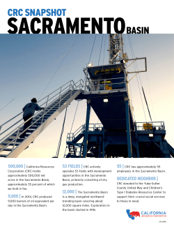


© Copyright 2026