1. No category

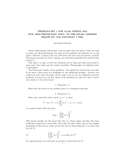
An optimal iterative solver for linear systems
arising from SFEM approximation of diffusion
equations with random coefficients
David Silvester and Pranjal
March 2015
MIMS EPrint: 2015.20
Manchester Institute for Mathematical Sciences
School of Mathematics
The University of Manchester
Reports available from:
And by contacting:
http://www.manchester.ac.uk/mims/eprints
The MIMS Secretary
School of Mathematics
The University of Manchester
Manchester, M13 9PL, UK
ISSN 1749-9097
AN OPTIMAL ITERATIVE SOLVER FOR LINEAR SYSTEMS
ARISING FROM SFEM APPROXIMATION OF DIFFUSION
EQUATIONS WITH RANDOM COEFFICIENTS
DAVID SILVESTER† AND PRANJAL‡
Abstract. This paper discusses the design and implementation of efficient solution algorithms
for symmetric linear systems associated with stochastic Galerkin approximation of elliptic PDE
problems with correlated random data. The novel feature of our iterative solver is the incorporation of
error control in the natural “energy” norm in combination with an effective a posteriori estimator for
the PDE approximation error. This leads to a robust and optimally efficient stopping criterion: the
iteration is terminated as soon as the algebraic error is insignificant compared to the approximation
error.
Key words. Stochastic Galerkin approximation, PDEs with random data, parametric operator
equations, a posteriori error analysis, iterative solvers, MINRES, optimal preconditioning.
AMS subject classifications. 35R60, 65C20, 65N30, 65N15.
1. Introduction. Stochastic spectral finite element methods are becoming popular for the numerical solution of steady-state diffusion problems whose permeability
coefficients are random fields. Galerkin approximation of the probabilistic dimension
of the PDE coupled with the finite element discretization in space gives rise to a
single linear(ized) system of equations whose coefficient matrix is symmetric positive
definite but is ill-conditioned with respect to the discretization parameters. Since
the coefficient matrix has a well-defined sparse structure, iterative solution methods can still be extremely effective. While preconditioned conjugate gradient (CG)
methods are commonly used for this purpose, we will focus on the classic MINRES
algorithm of Paige & Saunders [11] in this work. Specifically we will develop a new
solver for discretized diffusion problems with uncertain coefficients by extending the
EST MINRES algorithm developed for discrete saddle-point systems by Silvester &
Simoncini in [14]. The extended algorithm has two important features. First, the use
of a block preconditioner which will guarantee convergence independent of the problem parameters, and second, the use of a stopping criterion for the iterative solver
which balances the approximation error with the algebraic error. The latter requires
a reliable a posteriori error estimation technique for computing the approximation
error. The specific implementation discussed in this paper builds on the energy error
estimation framework developed by Bespalov et al. in [3].
Wathen [15] observed that numerical finite element approximation of PDEs endows the problem with a ‘natural norm’ that is determined by the specific approxi(k)
mation space. If u, uh , uh are the true solution, the Galerkin solution and algebraic
solution at the kth step (k = 0, 1, . . .) of the iterative solver respectively, then it is
(k)
shown that the ‘natural norm’ on the total error (u − uh ) at the kth step of iteration consists of two parts—the natural norm of the true approximation error (u − uh )
(k)
and the natural norm of the algebraic error (uh − uh ). Note that the total error
is actually the approximation error at the kth step of the iteration. For symmet‡ School of Mathematics, University of Manchester, Manchester, M13 9PL, United Kingdom,
[email protected]
† School of Mathematics, University of Manchester, Manchester, M13 9PL, United Kingdom,
[email protected]
1
ric positive-definite linear systems the ‘natural norm’ is the underlying energy norm.
Unfortunately, computing errors in the energy norm is anything but straightforward.
The preconditioned MINRES algorithm minimizes the norm of the residual of
the linear algebra system in terms of a norm that involves the preconditioner. This
‘surrogate norm’ is monotonically decreasing and is readily computable. Thus, the
choice of preconditioner is important for two different reasons. First for accelerating
convergence, and second, for ensuring that the convergence criterion matches the
‘natural norm’ of the discrete problem. In order to determine the stopping criterion
of the iterative solver, we must balance this energy norm of the algebraic error with
the energy norm of the approximation error at that step of iteration. Our stopping
criterion provides an inbuilt tolerance for the solver by balancing the approximation
error and the algebraic error. In this sense our solver is optimal.
The target linear algebra problem is set up in section 2 and the natural (energy)
norm is identified. This section also contains an overview of preconditioned MINRES
and develops the rationale for our stopping methodology. In section 3 we present a
set of computational results that can be reproduced using the S-IFISS toolbox [2]
and which confirm the effectiveness of our optimal stopping strategy. Throughout the
discussion, k · k , (·, ·) , R will denote the ℓ2 norm, the ℓ2 inner product and the set of
real numbers respectively.
2. Parameter dependent linear systems. The goal of this work is to develop
effective methods for solving parameterized symmetric linear systems of equations of
the form
(2.1)
A(y) u(y) = f,
where the entries in the matrix A ∈ Rn×n (and hence the solution vector u) depend
on a set of m parameters y = [y1 , y2 , . . . , ym ]T . Working in a statistical setting the
parameters might represent independent observations of uniform random variables
taking values in a bounded interval [a, b]. In practice the parameter dependence is
often taken to be linear, in which case we can decompose the coefficient matrix so
that
(2.2)
A(y) = A0 + σ
m
X
yk Ak ,
k=1
where A0 ∈ Rn×n might be associated with the mean of the coefficients and the
parameter σ > 0 might represent the standard deviation of the fluctuations. In
typical applications, the matrix A0 will be positive definite, but the matrices Ak may
be indefinite. In such cases, A(y) can only be guaranteed to be invertible when σ is
small enough. We will return to this issue later.
Symmetric systems of this type arise in the solution of linear elliptic partial differential equations with random coefficients. An example might be a heat conduction
problem in a region containing m different materials: each having thermal conductivity coefficient that is not known precisely. Discretization of such a PDE problem
(for example, using finite element approximation in space) typically leads to a linear
algebra system with a coefficient matrix of the form (2.2).
Classical Monte-Carlo (MC) methods are traditionally used to produce sample
solutions from independent realisations of parameter inputs. Statistics of the stochastic solution may then be generated by postprocessing the sample solutions. Although
they are robust and easily parallelizable, MC sampling can be an incredibly inefficient
2
use of computational resources, especially when solving large scale models where a
single deterministic solve of the original system is computationally expensive. An efficient alternative to MC sampling is to use a stochastic Galerkin method. These first
appeared in the engineering literature in the 1990s (see Ghanam & Spanos [6]) and
have been extensively studied over the last decade (see, for example, Deb et al. [4],
Babuska et al. [1]). Using this approach, the parameters are approximated by multivariate polynomials (Legendre polynomials in the case of uniform random variables)
of total degree p. Each solution coefficient is then written as a linear combination of
the polynomial basis functions
n
ui = u1i ξ1 + u2i ξ2 + . . . + ui ξ ξnξ
(2.3)
and the system is projected (in a least-squares sense) to give the best approximation
nξ
to the solution u from a finite-dimensional subspace Sp = span{ξj }j=1
. The Galerkin
projection process leads to the linear algebra system
(2.4)
A0 X + σ
m
X
Ak XGk = F
k=1
where X is the n × nξ matrix of the unknown coefficients uji and Gk is the weighted
Gram matrix associated with the kth parameter. Note that writing x = vec(X) leads
to an equivalent high-dimensional system (of dimension n · nξ ) with a characteristic
Kronecker product structure
P
(2.5)
Ax = f ⇐⇒ I ⊗ A0 + σ m
k=1 Gk ⊗ Ak x = f .
2.1. A model PDE problem. The simplest example of a problem that fits into
the framework above is the model of a diffusion process in a spatial domain D ⊂ Rd ,
with an isotropic permeability tensor K = κI where κ : D × Γ → R is parameterized
by m i.i.d. centred random variables, so that
(2.6)
κ(x, y1 , . . . , ym ) = µ(x) +
m
X
ψk (x) yk .
k=1
Here µ(x) is the mean value of the permeability coefficient at the point x ∈ D, yk ∈ Γk
is the image of the kth random variable, Γ = Γ1 × · · · × Γm and {ψk }m
k=1 are given
functions defined on D. The associated solution u(x, y) : D × Γ → R satisfies
(2.7a)
(2.7b)
(2.7c)
−∇ · K(x, y) ∇ u(x, y) = f (x),
u(x, y) = g(x),
K(x, y) ∇ u(x, y) · ~n = 0,
x ∈ D ⊂ Rd , (d = 2, 3), y ∈ Γ,
x ∈ ∂DD , y ∈ Γ,
x ∈ ∂DN = ∂D\∂DD , y ∈ Γ,
almost surely, where ∂DD , ∂DN are the Dirichlet and the Neumann part of the
boundary of D, and f and g are given deterministic functions.
The variational formulation of (2.7) is associated with the space W of functions
that are zero for all realizations on the Dirichlet boundary, and whose ‘stochastic
energy’ (defined later) is finite. The goal is to find u such that u − g ∈ W satisfies
Z
Z
(2.8)
K(x, y) ∇u(x, y) · ∇w(x, y) dx =
f (x)w(x, y) dx
D
D
3
for all w ∈ W , where h·i denotes the expected value of a multivariate random variable
defined on the space1 (Γ, B(Γ), π) with joint probability density function ρ(y) defined
on the product set Γ. It can thus be restated as: find u − g ∈ W such that
Z
Z
Z
Z
ρ(y) f (x)w(x, y) dx dy,
ρ(y) K(x, y) ∇u(x, y) · ∇w(x, y) dx dy =
(2.9)
Γ
Γ
D
D
for all w ∈ W . Note that the left side of (2.9) characterises the energy norm
Z
Z
2
ρ(y) K(x, y) |∇w(x, y)|2 dx dy,
(2.10)
kwkW =
Γ
D
so that the solution space is W = {u : kukW < ∞, u|∂DD ×Γ = 0} = H01 (D) ⊗ L2 (Γ).
A measure that will be equally important later is the energy norm of the solution
when the permeability coefficient is given by the mean field, that is
Z
Z
Z
2
2
ρ(y) µ(x) |∇w(x, y)| dx dy =
(2.11) kwk2E =
µ(x) |∇w(x, y)| dx .
Γ
D
D
Identifying the form of the (‘natural’) energy norms of the finite-dimensional version
of (2.8) is the first step towards expressing the energy norm of the algebraic error in
terms of a computable norm of the algebraic residual. The key point here is that the
two norms are equivalent whenever the formulation (2.8) is well posed (see [3]); that
is, there exist positive constants λ and Λ such that
(2.12)
λkwk2W ≤ kwk2E ≤ Λkwk2W
∀w ∈ W.
Galerkin approximation of (2.9) is associated with choosing finite dimensional
subspaces of the component spaces, that is Xh ⊂ H01 (D) and Sp ⊂ L2 (Γ) so that
Wh,p = H01 (D) ⊗ L2 (Γ). Full details can be found in [3] or [10, section 9.5]. When
generating test problems using the S-IFISS toolbox [2], the spatial domain D is twodimensional and the approximation is either piecewise bilinear (Q1 ) or biquadratic
(Q2 ) on a rectangular grid. This leads to sparse (stiffness) matrices A0 and Ak in
(2.4) and (2.5). In contrast, the parameter approximation space Sp is composed of
(multivariate) gobal polynomials, as in (2.3). For this space, it is sensible to choose a
nξ
basis set {ξj }j=1
that is orthogonal with respect to the probability measure π. This
leads to sparse matrices Gk (G0 = I, at most two nonzeros in any row otherwise) and
means that matrix-vector products with the coefficient matrix A in (2.5) are cheap
to compute—an essential ingredient for an effective iterative solver.
2.2. A fast iterative solver. Looking at the structure of our target system
(2.5) it is clear that the positive-definite matrix M− 1 = I ⊗ A0 will give an effective
approximation of A whenever σ is small relative to kA0 k. The use of M as a preconditioner for the system (2.5) will be a key component of our iterative solution strategy.
(In the stochastic Galerkin literature, this is sometimes referred to as mean-based
preconditioning.) Since I ⊗ A0 is a block-diagonal matrix, the action of its inverse
can be effected by a single sparse factorisation (of A0 ) followed by a nξ forward and
backward substitutions. Characterising a precise stopping criteria for our solver will
require accurate estimates of Rayleigh quotient bounds θ, Θ satisfying
(2.13)
1 The
θ≤
xT A x
≤ Θ,
xT M− 1 x
∀x ∈ Rn·nξ .
triple (Γ, B(Γ), π) is assumed to define a probability space, see Lord et al. [10, section 4.1].
4
An analysis of the spectral equivalence of M− 1 and A for our model PDE problem
can be found in Powell & Elman [13]. Note that since (2.12) is the infinite dimensional
analogue of (2.13), we know that λ ≤ θ and Θ ≤ Λ. This is not useful information in
general, since a priori estimates of λ and Λ are pessimistic and/or hard to find. To
address this, an effective way of computing estimates of θ and Θ on-the-fly will be
presented in section 2.4.
Solving our target system (2.5) using MINRES requires an initial vector x(0) , and
computes a sequence of iterates x(1) , x(2) , . . . from the shifted Krylov space
(2.14)
x(0) + span {r(0) , Ar(0) , . . . , A(k − 1) r(0) },
where r(0) = f − Ax(0) is the initial residual and k is the iteration number . The
characteristic feature of MINRES (see Liesen & Strakos [9, chap. 2]) is that the iterate
x(k) minimizes the Euclidean (ℓ2 ) norm k · k of the corresponding residual r(k) over
the shifted Krylov space r(0) + span {Ar(0) , A2 r(0) , . . . , Ak r(0) }.
The convergence estimate for unpreconditioned MINRES resulting from the minimum residual criteria is the optimal polynomial estimate
(2.15)
kr(k) k ≤
min
pk ∈ Πk , pk (0) = 1
max |pk (λj )| kr(0) k,
j
where Πk is the set of real polynomials of degree less than or equal to k and {λj }
are the eigenvalues of A (see Elman et al. [5, p. 191]). Let M be the mean-based
preconditioner for the system (2.5). Since M is a (symmetric) positive definite matrix,
we can write M− 1 = HH T and consider the preconditioned system
(2.16)
H− 1 A H− T y = H− 1 f,
y = H T x.
Clearly, any solution to (2.5) is also a solution to (2.16) and vice-versa. If MINRES
is applied to the symmetric system (2.16) then kH − 1 r(k) k will be minimized over the
k
space H − 1 (r(0) + span {AMr(0) , (AM)2 r(0) , . . . , (AM) r(0) }) at the kth iteration.
In fact, we have
(2.17)
kH − 1 r(k) k2 = kr(k) k2M = (r(k) )T M r(k) .
So, for preconditioned MINRES the convergence estimate analogous to (2.15) is
(2.18)
kr(k) kM
≤
kr(0) kM
min
pk ∈ Πk , pk (0) = 1
max |pk (λj )|,
j
where λj are the eigenvalues of the coefficient matrix H − 1 A H − T in (2.16). Note
that, from the similarity transformation, MA = H − T (H − 1 A H − T ) H T it follows
that λj are also the eigenvalues of MA. (Note that H is not needed in actual
computation—one only requires the action of M on a vector.) The optimal bound in
(2.18) can be weakened to a bound over the fixed interval [λ, Λ] by using the Rayleigh
quotient bounds on the eigenvalues of the preconditioned matrix in (2.13),
(2.19a)
(2.19b)
kr(k) kM
≤
min
max |pk (z)|
pk ∈ Πk , pk (0) = 1 z∈[θ,Θ]
kr(0) kM
≤
min
max |pk (z)| =: ρk .
pk ∈ Πk , pk (0) = 1 z∈[λ,Λ]
This implies that, when applied to our model problem, the preconditioned MINRES
iteration is guaranteed to satisfy a prescibed residual error tolerance in a fixed number
of iterations. The convergence rate of the solver will thus be bounded independently
of the stochastic Galerkin discretization parameters h and p.
5
2.3. An optimal stopping criterion. The real goal is to bound the norm of
the energy error in terms of the preconditioned residual norm that is minimised at
every step of MINRES. To this end, if r(0) is the initial residual and r(k) is the residual
at the kth iteration step, then inverting the eigenvalue bounds in (2.13) gives
T
T
(2.20)
(r(k) ) A− 1 r(k)
(r(0) ) A− 1 r(0)
1
,
≤
T
Θ
(r(0) ) M r(0)
T
(r(k) ) M r(k)
≤
1
,
θ
The algebraic error at the kth step is e(k) = x − x(k) = A− 1 r(k) , thus
(2.21)
T
T
ke(k) k2A = (e(k) ) A e(k) = (r(k) ) A− 1 r(k) = kr(k) k2A− 1 .
Combining (2.21) with (2.20) and (2.19b) gives the bounds
r
r
Θ kr(k) kM
Λ
ke(k) kA
≤
≤
(2.22a)
ρk
(0)
(0)
θ kr kM
λ
ke kA
1
(2.22b)
ke(k) kA ≤ √ kr(k) kM .
θ
The quantity √1θ kr(k) kM will be called the algebraic error bound in the rest of the
paper.
To devise the optimal stopping criterion, we make the premise that the algebraic
error at a given step of the iteration cannot be worse than the approximation error at
that step. To see what this means in the context of our model problem let uh − g ∈
Wh,p be the approximation to the PDE solution u. Then the vector x solving (2.5) will
be the coordinate vector of uh with respect to a chosen ordered basis. Next, let x(k)
be the coordinate vector at the kth iteration of the algebraic solver. Corresponding
(k)
to this kth iterate one can form the kth approximation uh and estimate the (mean)
(k)
energy error ku − uh kW a posteriori (for example, by using the energy estimator
developed in [3]). That is, one can compute η (k) satisfying
C
∼ O(1).
c
Combining the triangle inequality with Galerkin orthogonality gives the decomposition into the Galerkin solution approximation error and the algebraic error,
(2.23)
(2.24)
(k)
c η (k) ≤ ku − uh kE ≤ C η (k) ,
(k)
(k)
ku − uh k2E = ku − uh k2E + kuh − uh k2E .
Thus, assuming the a posteriori error estimates η and η k are close estimates of
the true approximation error and the approximation error at the kth iteration step,
respectively, (2.24) can be rewritten as
(2.25)
(k)
η (k) ≃ η + kuh − uh kE ,
{z
}
|
k = 0, 1, 2, . . .
ke(k) kA
Our iteration procedure can thus be looked upon as that of constructing a sequence,
{η (k) }, which converges to η. An efficient stopping point is the point when the contribution of the energy norm of the algebraic error to the sum in (2.25) becomes
insignificant. In the light of (2.22b) our preconditioned MINRES iteration will be
stopped at iteration k ∗ , the smallest value of k for which
1
√ kr(k) kM ≤ η (k) .
(2.26)
θ
A clever way of estimating the constant θ on the fly will be discussed next.
6
2.4. A posteriori estimation of the norm equivalence bounds. As already
mentioned, MINRES generates a sequence of approximations x(k) , k = 1, 2, . . . from
a shifted Krylov space such that the residual r(k) = f − Ax(k) is minimized. Let
us suppose that {w(1) , . . . , w(k) } is a set of orthonormal vectors spanning the kdimensional Krylov space, with w(1) = f /kf k, and let Wk = [w(1) , . . . , w(k) ]. These
basis vectors can be generated iteratively using the recurrence:
(2.27)
AWk = Wk Tk + tk+1,k w(k+1) eTk =: Wk+1 T k ,
where ek is the kth vector of the canonical basis and Tk is a tridiagonal symmetric matrix containing the orthogonalization coefficients; full details can be found in
Greenbaum [8, sect. 2.5]. Using (2.27) leads to the following characterisation of the
iterate, x(k) = Wk y(k) ,
(2.28)
r(k) = f − Ax(k) = Vk+1 e1 kf k − T k y(k) .
The minimizing solution x(k) may then be found by solving the least squares problem
miny ke1 kf k − T k yk. The Lanczos relation in (2.27) can also be used to show that
Tk = WkT AWk so that the eigenvalues of Tk , also known as the Ritz values,2 provide
approximations to the eigenvalues of A (or of MA if the matrix is preconditioned).
In our setting we would like to estimate the extremal eigenvalues θ, Θ of the preconditioned matrix associated with (2.13) on the fly. What works in our favour is the
fact that extremal Ritz values can be readily computed at every step of the MINRES
iteration and that they provide accurate estimates of the extremal eigenvalues, even
when k (the number of iterations) is relatively small. This key aspect is discussed
in Parlett [12, chap. 13]. The efficiency of this eigenvalue estimation strategy will be
confirmed by the computational experiments presented in the next section.
3. Computational results. To give a proof of concept, the results of computational experiments when the stopping test (2.26) is applied to systems of the form
(2.1) derived from the model PDE problem (2.7) will be presented in this section.
Representative systems (2.5) can be generated for this purpose using the S-IFISS
toolbox [2]. Our test problem is defined on a square domain D = (− 1, 1) × (− 1, 1)
with source function f (x) = 81 (2 − x21 − x22 ) and zero Dirichlet condition everywhere
on the boundary. The spatial approximation space Xh is a piecewise bilinear finite
element space on a uniform of grid of square elements (here h > 0 denotes the length
of each element edge). We will present results for h = 21 − l , (l = 3, 4, 5, 6).
The S-IFISS software generates a diffusion coefficient κ in (2.6) with uniform
random variables defined on Γk = [−1, 1], and the parameter approximation space
Sp is spanned by complete polynomials of degree p. The mean field
√ in the expansion
(2.6) is constant, µ(x) = 1, and the spatial functions ψk = 3λk ϕk in (2.6) are
associated with eigenpairs {(λk , ϕk )}m
k=1 of the (separable) covariance operator
1
(3.1)
C(x, x′ ) = σ 2 exp − kx − x′ kℓ1 , x, x′ ∈ D ⊂ R2 ,
2
where σ denotes the standard deviation, and the correlation length is 2. We note that
the resulting model problem is essentially the same as that considered in [4] and [13].
2 The idea of exploiting the Lanczos connection was introduced by Silvester & Simoncini [14] in
the context of saddle-point problems. The main difference is that harmonic Ritz values are used
in [14] in place of Ritz values—estimates of interior eigenvalues are needed in the saddle-point case.
7
2
2
10
10
√1 kr(k) kM
θ
kr(k) kM
0
10
η (k)
η
−2
10
√1 kr(k) kM
θ
kr(k) kM
1
10
η (k)
η
0
10
−1
10
−4
10
−2
10
−6
10
−3
10
−4
−8
10
0
5
10
iteration number
10
15
0
5
10
15
iteration number
20
25
Fig. 1. Errors vs iteration number for optimally preconditioned MINRES for the model PDE
problem with h = 1/32, m = 5, p = 3 | σ = 0.3 (left), σ = 0.5 (right).
2
2
10
10
√1 kr(k) kM
θ
kr(k) kM
1
10
η (k)
η
0
10
η (k)
η
0
−1
−1
10
−2
−2
10
10
−3
−3
10
10
−4
0
1
10
10
10
10
√1 kr(k) kM
θ
kr(k) kM
−4
5
10
15
20
iteration number
25
10
0
10
20
iteration number
30
Fig. 2. Errors vs iteration number for optimally preconditioned MINRES for the model PDE
problem with m = 7, p = 3 for σ = 0.5 | h = 1/8 (left), h = 1/16 (right).
The discretised problems were set up by running stoch diff testproblem. The
resulting algebraic system was solved by calling a new function stoch est minres.
A reference solution was computed in each case by turning off our optimal stopping
criterion in stoch est minres, and solving the discrete system with a preconditioned
residual reduction tolerance of 1e-14. We will compare the reference solution x
∗
obtained in this way with the result x(k ) computed using the optimal stopping test.
The starting vector x(0) is always generated using the MATLAB function rand.
Some representative results are presented in Figures 1 and 2. These figures show
the evolution of the residual error krkM together with the algebraic error bound; with
θ estimated at each step k using the strategy outlined in section 2.4. The approxima8
tion error η (k) is also plotted at each step: it can be seen to converge to the estimate
η associated with the reference solution. Note that we take 9 additional iterations
after convergence to ensure that we have stopped at the right place. The results in
Figure 1 show that the solver takes longer to converge when the standard deviation is
increased (all other parameters being kept constant). This is to be expected since λ
in (2.12) (and θ in (2.13) become increasingly negative when σ is increased.3 (Indeed
our PDE problem is not well posed for σ > σ ∗ ≈ 0.55). The iteration automatically
stops after 9 iterations when σ = 0.3, but takes about twice as may iterations when
σ = 0.5. The results in Figure 2 illustrate that the convergence of the solver is essentially independent of the spatial discretization (assuming that m and σ are kept
fixed). This is what we mean by fast convergence!
The number of iterations needed to satisfy the optimal stopping test (2.26) is
compared in Tables 1–3 with the number (ktol ) needed to satisfy a fixed (absolute)
tolerance of 1e-3. These tables provide additional evidence that, for fixed stochastic
parameters, the number of iterations stays bounded as the spatial grid is increasingly refined. This boundedness is also evident in the tabulated extremal Ritz values
computed at iteration k ∗ .
Table 1
Iteration counts and Rayleigh quotients estimates for the case σ = 0.3 m = 5 and p = 3.
l
ktol
k∗
θ∗
Θ∗
3
4
5
6
8
9
10
10
6
7
8
9
0.5276
0.4833
0.4734
0.4708
1.5044
1.5257
1.5283
1.5311
Table 2
Iteration counts and Rayleigh quotients estimates for the case σ = 0.5 m = 5 and p = 3.
l
ktol
k∗
θ∗
Θ∗
3
4
5
6
17
20
21
22
11
14
16
17
0.1358
0.1110
0.1042
0.1029
1.8789
1.8941
1.9032
1.9045
Table 3
Iteration counts and Rayleigh quotients estimates for the case σ = 0.5 m = 7 and p = 3.
l
ktol
k∗
θ∗
Θ∗
3
4
5
21
27
30
13
18
22
0.0908
0.0558
0.0413
1.9315
1.9590
1.9649
The stopping point Ritz estimates turn out to be extremely good approximations
of the actual extremal eigenvalues. This is evident in Figures 1 and 2 —the algebraic
bound curve is too close to the curve of the norm of the preconditioned residual for
3 Sharp bounds [1 − τ, 1 + τ ] for the Rayleigh quotient (2.13) are established by Powell & Elman
in [13, Theorem 3.8], where the factor τ is the sum of the norms kψk k∞ of the functions in (2.6).
These bounds suggest that convergence will also be affected if m is increased with σ kept fixed.
9
1.8
Actual eigenvalues
Ritz values
Actual eigenvalues
2
1.6
1.4
1.5
1.2
1
1
0.8
0.5
0.6
Ritz values
0.4
0
5
10
iteration number
0
0
15
5
10
15
iteration number
20
25
Fig. 3. Computed Ritz values for the model PDE problem with m = 5, p = 3 | h = 1/16 and
σ = 0.3 (left) h = 1/8 and σ = 0.5 (right).
the first few iterations but the two curves rapidly become parallel as θ(k) converges
to θ. This is also illustrated by the plots in Figure 3 showing the convergence of the
Ritz values. A final observation is that there is no sign of any “ghost” eigenvalues
(see Golub & van Loan [7, p. 566, sect. 10.3.5]) in any of these computations.
REFERENCES
[1] I. M. Babuˇ
ska, R. Tempone, and G. E. Zouraris, Galerkin finite element approximations of
stochastic elliptic partial differential equations, SIAM J. Numer. Anal., 42 (2004), pp. 800–
825.
[2] Alex Bespalov, Catherine Powell, and David Silvester, S-IFISS ver. 1.0, September
2013. available online at http://www.manchester.ac.uk/ifiss/s-ifiss1.0.tar.gz.
, Energy norm a posteriori error estimation for parametric operator equations, SIAM J.
[3]
Sci. Comput., 36 (2014), pp. A339–A363. http://dx.doi.org/10.1137/130916849.
[4] M. K. Deb, I. M. Babuˇ
ska, and J. T. Oden, Solution of stochastic partial differential equations using Galerkin finite element techniques, Comput. Methods Appl. Mech. Engrg, 190
(2001), pp. 6359–6372.
[5] Howard Elman, David Silvester, and Andy Wathen, Finite Elements and Fast Iterative
Solvers: with Applications in Incompressible Fluid Dynamics, Oxford University Press,
Oxford, UK, 2014. Second Edition.
[6] Roger G. Ghanem and Pol D. Spanos, Stochastic finite elements: a spectral approach,
Springer-Verlag, New York, 1991.
[7] Gene Golub and Charles Van Loan, Matrix Computations, The John Hopkins University
Press, Baltimore, USA, 2013. Fourth Edition.
[8] A. Greenbaum, Iterative Methods for Solving Linear Systems, SIAM, Philadelphia, PA, 1997.
¨ rg Liesen and Zdenek Strakos, Krylov Subspace Methods, Principles and Analysis, Oxford
[9] Jo
University Press, Oxford, UK, 2012.
[10] Gabriel J. Lord, Catherine E. Powell, and Tony Shardlow, An Introduction to Computational Stochastic PDEs, Cambridge University Press, Cambridge, UK, 2014.
[11] C. C. Paige and M. A. Saunders, Solution of sparse indefinite systems of linear equation,
SIAM J. Numer. Anal., 12 (1975), pp. 617–629.
[12] B. N. Parlett, The Symmetric Eigenvalue Problem, SIAM, Philadelphia, PA, 1998.
[13] Catherine E. Powell and Howard C. Elman, Block-diagonal preconditioning for spectral
stochastic finite-element systems, IMA J. Numer. Anal., 29 (2009), pp. 350–375.
[14] David J. Silvester and Valeria Simoncini, An optimal iterative solver for symmetric indefinite systems stemming from mixed approximation, ACM Trans. Math. Softw., 37 (2011).
http://dx.doi.org/10.1145/1916461.1916466.
[15] A. J. Wathen, Preconditioning and convergence in the right norm, Int. J. Comput. Math., 84
(2007), pp. 1199–1209.
10