
- White Rose Etheses Online
The Identification and
Characterisation of Microbes in
Complex Environments
Alexander L.B. Leach
Doctor of Philosophy
University of York
Biology
September, 2013
Abstract
The practice of genetically identifying microbes has become increasingly commonplace in
recent decades. Since Carl Woese discovered the utility of small subunit ribosomal RNA,
for identifying an organism and Frederick Sanger introduced his method for de novo sequencing, the throughput of producing taxonomically relevant sequence information has
risen exponentially. Small subunit rRNA has been invaluable in preliminarily identifying
microbial organisms. With just a fragment of this single gene sequence, evolutionary
distances between organisms can be inferred and microbes identified. A novel software
pipeline - SSuMMo - was designed and developed to help identify organisms present in
complex microbial communities, using datasets produced by the latest high-throughput
sequencing technologies. SSuMMo was stringently tested for accuracy, speed and efficacy
on a variety of datasets to assess its utility when analysing real sequence datasets, generated
from both 16S rRNA primer-targeted and whole genome shotgun sequencing experiments.
Sequence length is often compromised with recent high-throughput sequencing technologies, so simulations were performed to ascertain the best candidate regions for primer
design on the 16S rDNA gene. The software is further demonstrated on public sequence
datasets generated from sequencing the human oral and gut microbiomes. Our analyses
show that SSuMMo is a viable software package for identifying species present in complex
communities, particularly with primer-targeted high-throughput sequence datasets.
iii
Contents
Abstract
iii
List of Tables
ix
List of Figures
x
List of Code Listings
xii
List of Accompanying Material
xiii
Acknowledgements
xv
Declaration
1
xvii
Introduction
1
1.1
Aims . . . . . . . . . . . . . . . . . . . . . . . . . . . . . . . . . . . . . . . . .
2
1.2
Motivation . . . . . . . . . . . . . . . . . . . . . . . . . . . . . . . . . . . . . .
2
1.3
The First Signs of Microbial Life . . . . . . . . . . . . . . . . . . . . . . . . . .
4
1.3.1
Darwin’s struggle . . . . . . . . . . . . . . . . . . . . . . . . . . . . .
6
1.3.2
A (re-)revolution of biological philosophy . . . . . . . . . . . . . .
7
1.3.3
The Hereditary mechanism . . . . . . . . . . . . . . . . . . . . . . .
9
1.3.4
Distance of difference . . . . . . . . . . . . . . . . . . . . . . . . . .
11
v
1.4
2
System and Methods
12
19
2.1
Hidden Markov Models in Biological Systems . . . . . . . . . . . . . . . . . . .
20
2.2
Building the SSuMMo database of HMMs . . . . . . . . . . . . . . . . . . . . .
22
2.3
Associating names with taxonomic rank . . . . . . . . . . . . . . . . . . . . .
23
2.4
Assigning novel sequences to taxa . . . . . . . . . . . . . . . . . . . . . . . .
24
2.5
Accuracy Testing . . . . . . . . . . . . . . . . . . . . . . . . . . . . . . . . . .
24
2.5.1
HMM Testing . . . . . . . . . . . . . . . . . . . . . . . . . . . . . . . 24
2.5.2
Sequence length versus Assignment Accuracy . . . . . . . . . . . .
25
2.5.3
SSU rRNA hypervariable region accuracy . . . . . . . . . . . . . .
25
2.6
Optimizing SSuMMo for speed . . . . . . . . . . . . . . . . . . . . . . . . . . .
26
2.7
Comparative metagenomics . . . . . . . . . . . . . . . . . . . . . . . . . . . .
26
2.8
Assigning Training Sequences to Taxa . . . . . . . . . . . . . . . . . . . . . . .
27
2.9
Training the Database of HMMs . . . . . . . . . . . . . . . . . . . . . . . . . .
28
2.10 Matching Names Between ARB and NCBI Taxonomy Databases . . . . . . . . .
28
2.11
Testing Accuracy . . . . . . . . . . . . . . . . . . . . . . . . . . . . . . . . . .
30
2.12
Importing and Exporting Trees to IToL . . . . . . . . . . . . . . . . . . . . . .
31
2.13
Calculating Biodiversity Indices . . . . . . . . . . . . . . . . . . . . . . . . . .
31
2.14 Finding Taxa and their Lineage . . . . . . . . . . . . . . . . . . . . . . . . . . .
33
Plotting Tabular Data on to Trees . . . . . . . . . . . . . . . . . . . . . . . . .
34
2.16 Inferring Sequence Conservation . . . . . . . . . . . . . . . . . . . . . . . . .
34
Comparing Processing Times Against BLAST . . . . . . . . . . . . . . . . . . .
35
2.15
2.17
3
Genetic Sequencing since the 1970s . . . . . . . . . . . . . . . . . . . . . . . .
Identifying Microbes with Small Subunit ribosomal RNA
37
3.1
Taxon Identification with SSuMMo . . . . . . . . . . . . . . . . . . . . . . . . .
38
3.2
Results and Discussion . . . . . . . . . . . . . . . . . . . . . . . . . . . . . . .
43
vi
4
Assignment Accuracy . . . . . . . . . . . . . . . . . . . . . . . . . .
3.2.2
Software comparisons . . . . . . . . . . . . . . . . . . . . . . . . . . 47
3.2.3
Sequence Windows and Primer Design . . . . . . . . . . . . . . . . 48
3.2.4
Biological Diversity . . . . . . . . . . . . . . . . . . . . . . . . . . . 49
3.2.5
Repository Annotation Effects . . . . . . . . . . . . . . . . . . . . .
51
3.2.6
SSuMMo for database curation . . . . . . . . . . . . . . . . . . . .
52
Microbes Inhabiting the Human Microbiome
43
55
4.1
Aims . . . . . . . . . . . . . . . . . . . . . . . . . . . . . . . . . . . . . . . . .
56
4.2
Methods . . . . . . . . . . . . . . . . . . . . . . . . . . . . . . . . . . . . . . .
57
4.2.1
Sample Datasets . . . . . . . . . . . . . . . . . . . . . . . . . . . . .
59
Results . . . . . . . . . . . . . . . . . . . . . . . . . . . . . . . . . . . . . . . .
62
4.3
5
3.2.1
4.3.1
A core healthy microbiome . . . . . . . . . . . . . . . . . . . . . . . 62
4.3.2
Healthy and IBD-infected gut microbiotas . . . . . . . . . . . . . . 64
4.3.3
Gut microbiome differences relating to adiposity . . . . . . . . . . 67
4.3.4
Annotating WGS sequences . . . . . . . . . . . . . . . . . . . . . .
4.3.5
Gut microbiome diversity relating to geographic location . . . . . 76
Discussion
74
81
5.1
Sequence clustering methods . . . . . . . . . . . . . . . . . . . . . . . . . . .
82
5.2
Comparing microbiological community diversities . . . . . . . . . . . . . . . .
84
5.3
Summary . . . . . . . . . . . . . . . . . . . . . . . . . . . . . . . . . . . . . .
84
Appendix I
87
A1.1 Code Listings . . . . . . . . . . . . . . . . . . . . . . . . . . . . . . . . . . . .
87
A1.2 Tables . . . . . . . . . . . . . . . . . . . . . . . . . . . . . . . . . . . . . . . . 101
Nomenclature
103
vii
Bibliography
105
viii
List of Tables
3.1
SSuMMo annotation accuracies. . . . . . . . . . . . . . . . . . . . . . . . .
43
3.2
SSuMMo species mismatches. . . . . . . . . . . . . . . . . . . . . . . . . . . 46
3.3
SSuMMo vs. BLAST runtimes. . . . . . . . . . . . . . . . . . . . . . . . . . 48
4.1
Geographical human gut dataset statistics. . . . . . . . . . . . . . . . . . .
58
4.2
Healthy vs. IBD gut dataset statistics. . . . . . . . . . . . . . . . . . . . . . .
59
4.3
Analysis of Variance of biodiversity index calculations. . . . . . . . . . . . 66
4.4
SSuMMo assignment statistics of Human Microbiome sequence data. . . 69
A1.1 Biodiversity indices for geological datasets at different ranks. . . . . . . . . 101
ix
List of Figures
1.1
Shannon Entropy of DNA. . . . . . . . . . . . . . . . . . . . . . . . . . . . .
11
2.1
A simplified schematic of an Hidden Markov Model. . . . . . . . . . . . .
21
3.1
High level overview of A) SSuMMo annotation pipeline; and B) select
post-analysis programs. . . . . . . . . . . . . . . . . . . . . . . . . . . . . . .
39
3.2
Accuracy of SSuMMo assignments in SSU rRNA hypervariable regions. .
41
3.3
SSuMMo accuracy for antisense strands of hypervariable regions. . . . . . 42
3.4
Accuracy of SSuMMo compared with sequence length. . . . . . . . . . . . 44
3.5
Accuracy of Archaeal 16S rRNA sequences run through SSuMMo. . . . . 47
3.6
Counts of rRNA operon genes in Human Oral Microbiome Database. . . 50
4.1
Distribution of taxa up to genus specificity, present in the guts of 154 lean,
overweight and obese individuals, pooled by sequencing method and
BMI category. . . . . . . . . . . . . . . . . . . . . . . . . . . . . . . . . . . . 62
4.2
Gut microbiota of 99 healthy vs. 25 IBD-suffering individuals.
4.3
Body Mass Index vs. Firmicutes / Bacteroidetes ratio. . . . . . . . . . . . . 70
4.4
Biodiversity analyses of Lean, Overweight and Obese individuals’ gut
4.5
. . . . . .
65
microflora. . . . . . . . . . . . . . . . . . . . . . . . . . . . . . . . . . . . . .
71
Genera identified in Japanese guts, from WGS experiment. . . . . . . . . .
75
x
4.6
Biodiversity indices calculated for geographical datasets. . . . . . . . . . . 76
4.7
Rarefaction curves of 66 healthy individuals’ gut microbiota. . . . . . . . .
xi
77
List of Code Listings
A1.1 A Python script to plot informational entropy of a DNA sequence . . . .
A1.2 A shared module containing common plotting functions
87
. . . . . . . . . 88
A1.3 A Python script that calculates informational entropy from genomic DNA
sequence files . . . . . . . . . . . . . . . . . . . . . . . . . . . . . . . . . . . 90
A1.4 A Python script to extract sequences of interest from the Clinical Production Pilot Study (PPS) of the NIH Human Microbiome Project . . . . . . 100
xii
List of Accompanying Material
SSuMMo Documentation
API documentation, tutorial and installation instructions produced for the
SSuMMo software package, described in chapter 3.
This software was generated using Sphinx [Brandl, Georg, 2009], by extracting
documentation directly from source code, as well as using additional reStructured Text (rst) files, written specifically for the purpose of documenting the
source code packages.
xiii
Acknowledgements
I wish to thank the following for helping me on my way. . .
First and foremost, my supervisors James & Kelly, for their guidance, support
and confidence in me, since I began researching in York.
Members of my Training Advisory Committee: Gavin Thomas & Jon Pitchford, for their insight, encouragement and enthusiasm throughout my research.
The Burgess family for their philanthropism and faith in science. Their generosity provided the funds necessary to conduct the research contained herein,
as well as that of many other York biologists, both before and after my own.
The Trustees of the Holbeck Trust, for their shared contribution to my research
funding, as well as to others throughout the University.
My eldest brother Ben, for his generosity and the support he offers many
talented individuals.
My family, friends and departmental colleagues, who are too numerous to
mention individually, have helped me immeasurably in the struggle to remain
diligent, determined and vivacious.
Thank you, all!
xv
Declaration
I declare that this thesis is a presentation of original work and I am the sole
author. This work has not previously been presented for an award at this, or
any other, University. All sources are acknowledged as References.
Work in chapter 3 has largely already been published in Bioinformatics [2012]
and presented at the Nordic Archaeal [2011a] conference.
Work in chapter 4 has previously been presented at the Modelling & Microbiology [2011b] and SGM Autumn [2011c] conferences.
Leach, A.L.B., Chong, J.P.J. & Redeker, K.R. (2012). SSuMMo: rapid analysis,
comparison and visualization of microbial communities. Bioinformatics, 28,
679–686.
Leach, A.L.B., Chong, J.P.J. & Redeker, K.R. (2011a). A novel method for
phylotyping complex populations. Nordic Archaeal conference, Helskinki.
Leach, A.L.B., Chong, J.P.J. & Redeker, K.R. (2011b). Microbial community
auditing with ss-RNA. Searching for a core microbial community in the guts
of healthy humans. Modelling & Microbiology conference, Edinburgh.
Leach, A.L.B., Chong, J.P.J. & Redeker, K.R. (2011c). Searching for a core microbial community in the human gut microbiome. SGM Autumn conference,
York.
xvii
For Ben, James & Kelly
•
1
Introduction
Microbial life pervades all reaches of the Earth. As our understanding grows, so
too has its apparent ubiquity and number. From the bottom of oceans to clouds in the sky
[Sattler et al., 2001; Vetriani et al., 1999], microscopic life persists where we can just visit.
As more and more natural habitats are explored, so too do we acknowledge the unknown
forms of life that inhabit them. As way of example, in a single gram of soil, it is estimated
that there are up to twenty billion individual prokaryotes living therein [Whitman et al.,
1998]. Of those, less than one percent of species are purported to be cultivable [Amann
et al., 1995; Schloss & Handelsman, 2006].
The importance of microorganisms on Earth cannot be overstated. In their conquering
of the globe billions of years ago, it was they who formed the atmosphere that we now
require to live [Kasting & Siefert, 2002]. It was they who first learned how to harvest
energy from the sun, how to sense, swim [Blair, 1995] and even to communicate with
one another [Williams et al., 2007]. In a sense, to learn about microorganisms is to learn
about ourselves. In manipulating microorganisms, we can create fuel and medicine; food
and drink; life and death.
Since Koch’s postulates were founded in the 19th century [Falkow, 2004; Koch, 1890],
isolating microbes in pure culture has historically been one of the first steps taken in
attempting to understand a microorganism. In doing so, physiological and phenotypic
observations are made, providing knowledge of the organism in question. Since this is
1
recognised as impossible for a vast majority of organisms in natural environments, new
culture-independent methods have had to be developed. Many of these methods consist
of refinements, improvements and miniaturisation of DNA sequencing technologies,
used to determine the genetic information contained within and passed down between
generations of living organisms (see section 1.4).
1.1 Aims
This thesis begins with exploring how methods of microbiological inquiry arose and have
developed in human history, from identification of the first signs of microscopic life, to
the latest technologies used to inspect them. Computational tools were developed to assist
with analysing and visualising datasets resulting from such high-throughput sequencing
experiments and are presented herein. User manuals and library documentation, produced
as part of the software development process, are attached separately.
The overarching goals of the project are to create helpful and informative computational tools, to assist with identifying and characterising microbes in complex environments. As sequencing experiments become increasingly large and frequently created, it
is the aim of this project to create tools that may prove invaluable, in future analyses of
high-throughput sequencing data.
1.2 Motivation
Genetic sequencing has impacted and affected virtually all branches of contemporary
biology [Shendure & Aiden, 2012]. The scale at which the technology has developed
over the last decade has been unparalleled, in terms of speed, capacity and resolution
[Mardis, 2011; Metzker, 2009; Shendure & Ji, 2008]. Conversely, the cost of sequencing has
2
seen a rapid decline, shifting the main financial burden of sequencing experiments away
from generation of the sequence data itself, to practically every other stage of the process:
from collection of samples to storage of the resulting data [Shendure & Aiden, 2012].
The technical challenges of sequencing experiments have seen a similar shift, resulting
from the dramatic increase in dataset size. One of the remaining technical difficulties
regards manipulating resulting sequence data to provide meaningful insight from the
sheer quantity of genetic information produced [Nielsen et al., 2010]. Not only is technical
knowledge and skill required in using one of the many computational tools available, but
a huge amount of computational power and time is necessary to process the sequence
data [MacLean et al., 2009; Pop & Salzberg, 2008].
One of the many consequences of the sequencing revolution is the increased range
and scope of natural environments that can be investigated. While sequencing originally
had very limited coverage (see section 1.4), it is becoming increasingly common for
experiments to produce gigabases of DNA at a time (e.g. [Hess et al., 2011; Qin et al.,
2010]), with this upward trend unlikely to stop any time in the near future.
Although 100% genomic coverage is unlikely to be obtained from such densely populated environmental samples, the amount of raw data generated from single experiments
has still managed to overwhelm public data warehouses, to the extent that the National
Centre for Biotechnology Information (NCBI) announced in 2011 that, because of budget constraints, they would at some point have to stop supporting the Trace and Short
Read Archives (the ‘SRA’ - since renamed the “Sequence Read Archive”) [Galperin &
Fernández-Suárez, 2012]. Due to public demand, the NIH has since changed their stance
and has decided to continue funding the SRA, keeping in line with other consortia who
comprise the INSDC [Nakamura et al., 2013].
Although the NIH’s budget has only rarely seen decreases in its annual budget since
the 1970’s [Loscalzo, 2006], the recent technical innovations in DNA sequencing have
3
been improving faster than computer technologies have been able to keep up [Rothberg
et al., 2011]. Solutions to this problem include continually increasing the allocated budget
for computational infrastructure used to both analyse and store this mass of sequence
data. Another aim is to improve upon and develop new software for the job of both data
processing and storage [Fritz et al., 2011; Richter & Sexton, 2009].
1.3 The First Signs of Microbial Life
Biology has one of the longest and most illustriously documented histories in scientific
literature. Microbiology was a relatively recent introduction to the discipline, but can be
traced through the pages of history equally well. But what is a micro-organism? How can
they be identified and how, can they be told apart? These questions will be answered here
in the context of some important historical discoveries, before applying some classical
methodologies to contemporary datasets.
Nowadays, microbiological methods are used in a plethora of theoretical and applied
science, ranging from improving human health [Mitsuoka, 1990], to its detriment [Wheelis,
1998]; from biofuel production [Holder et al., 2011] to atmospheric cleansing [Falkowski
et al., 2008]; from manufacture of food and drink [Leroy & De Vuyst, 2004] to the
processing of waste [Tsai et al., 2007]. The use cases of microbes are now so widespread
that it is a wonder how the human race lived without recognising their existence for so
long. So when did the human race first become aware of microbial life?
“Microbe” and “microorganism” are fairly common terms nowadays, so a good place
to start might be the Oxford English Dictionary [2013], which contains entries and etymological records for both:
microbe, n.
An extremely small living organism, a microorganism; esp. a bacterium causing disease or
fermentation.
4
microorganism, n.
An organism so small as to be visible only under a microscope; esp. bacterium, fungus, or
alga.
For linguists and scientists alike, the common Greek ‘micro’ prefix is indicative of
something too small to see with the naked eye, exactly what the above dictionary definitions imply. This would also explain their relatively recent introduction to the English
language. The first known uses of each word date only back to 1880 [Holden, 2013], although microscopy had been practiced in England since the 17th century, when Robert
Hooke published Micrographia [1665], his notorious, illustrated book of observations
made under the microscope.
From this publication, Robert Hooke is recognised as the first to give a detailed
description of a microorganism; likely a fungus of the common Mucor genus [Gest, 2004;
Orlowski, 1991]. But it wasn’t until the next decade that the Dutch shopkeeper Antonie
van Leeuwenhoek first described unicellular microorganisms. In letters written in Dutch
to the Royal Society of London, he described what later became known to be protists,
as ‘animalcules’ or ‘little eels’, ‘very prettily moving’ in pepper-infused water [Gest, 2004;
Mazzarello, 1999; Porter, 1976; Smit & Heniger, 1975]. The fact that they were motile was
indication enough that they were alive, but little more insight could be learned about
microorganisms until two centuries later. This is understandable when considering the
accepted philosophies of the period, as well as the technical achievement of constructing
a microscope in the 17th century. Both Hooke and van Leeuwenhoek had to make their
microscope components themselves and van Leeuwenhoek chose to keep his methods a
close-guarded secret [Gest, 2004; Porter, 1976].
Other than morphological and physiological observations made under the microscope,
it wasn’t until the 20th century that micro-organisms could be distinguished by more
specific means. The 19th century did herald a series of novel techniques for isolating,
culturing and distinguishing certain bacteria based on physical appearance [Barnett, 2003;
5
Drews, 2000], but it still required more theoretical, philosophical and technical advance
before microorganisms could be distinguished by any quantitative means. Even macroorganisms - those lifeforms visible with the naked eye - which had been categorised based
on physiological properties since Aristotle (c. 384-322BC) [Gaarder, 1991] - could be given
no quantitative measure of relatedness until the 20th century.
1.3.1 Darwin’s struggle
Of course it was Darwin’s On the Origin on Species [Darwin, 1859] that provided some of
the first evidence for a theory of evolution, but it took time for this to become accepted.
Philosophers of the day were said mostly to be of the ‘essentialist’ school of thought, which
fundamentally contradicts the idea of evolution [Mayr, 1982]. Essentialism was introduced
by the well-renowned philosopher Plato (c. 428-437BC), a faithful student of Socrates,
whose ‘theory of ideas’ attempted to explain how individuals could be of the same species,
yet each individual of a species be different. Plato supposed that for every type of thing
that exists, be it living or otherwise, each has an eternal eide, or ‘essence’, of which we
perceive only imperfect manifestations. The essences would exist only in the ‘world of
ideas’, a place both eternal and immutable [Gaarder, 1991], while the observable forms
exist in the natural, sensory world. New species would therefore be an impossibility, as a
species’ ‘essence’ could not change or be created in the eternal world of ideas. This theory,
dubbed the “dead hand of Plato”, might explain what took mankind so long to accept the
theory of evolution [Dawkins, 2008, 2009; Mayr, 1959].
Ideas can evolve and so too, can species. After 2,000 years of Platoan, essentialist
thought and this began to be accepted. Darwin’s famous voyage on the Beagle provided
ample evidence supporting evolution, with natural selection as the mechanism in life’s
struggle to survive. But the conclusions his evidence led towards were hard for many to
accept, not only the ‘essentialists’, but creationists too [Dawkins, 2009]. Perhaps the most
6
astonishing conclusion, was that species on Earth are related, in a family tree that spans at
least the entirety of macroscopic life [Glansdorff et al., 2008; Woese, 1998].
At the turn of the 20th century, this was still far from accepted, however. The mechanisms by which to understand heredity were still a long way off, and a biological mechanism for evolution equally so. Only once these were discovered and understood, could a
method to measure the relatedness of species be found. It took another half-century for
the necessary breakthroughs to arrive, but the insight gained from Darwin’s work allowed
a new dawn of biological thought.
1.3.2
A (re-)revolution of biological philosophy
According to Mayr [1959], a shift in thought away from essentialism led to ‘populationism’, where types are not real, but are instead only averaged abstractions of individuals’
characteristics [Dawkins, 2008; Sober, 1980]. The theories are directly controvertible, as
Plato’s earlier philosophies assume the observable, sensory world we live in consists of
abstractions from eternal forms, whereas “for the populationist, the type (average) is an abstraction and only the variation is real” [Mayr, 1959]. Evolutionary theory undermines the
assumption in essentialism that species are static in nature, instead enforcing uniqueness
of individuals, concordant with Mayr’s populationism [Bradshaw, 2001].
This was an age-old argument dating again back to Aristotle, who was the first to
challenge Plato’s theory of ideas, claiming: “every change in nature [. . . ] is a transformation of substance from the ‘potential’ to the ‘actual’” [Gaarder, 1991]. So why then, did
Plato’s earlier philosophies dominate Aristotle’s up until the 19th century? The reason may
have been the so-called ‘neo-platonism’, said to have been re-introduced into Western
philosophy by Plotinus (c. 205-270), who brought Plato’s theory of ideas from Alexandria
to Rome, merging Plato’s theories into common theological beliefs regarding an eternal
soul [Gaarder, 1991]. Over 500 years after Aristotle, Western philosophy could be said
7
to have taken a step backward: a disputed philosophical reasoning was merged with
theological belief, simultaneously strengthening both modes of thought and enforcing a
preconception against evolution.
A key consideration in both Aristotelian and Darwinian theory, but missing from
Platonic, is time. Darwin understood that evolution in the visible world could only be
valid if physical changes occurred over “geological time-scales” [Gould, 1983]. Although
Aristotle wasn’t privy to the same information as Darwin when it came to geological
timescales, change of state is fundamentally a function of time. Furthermore, it remains
that what is ‘actual’ is only a subset of nature’s ‘potential’; natural environments dictate
what life has ‘potential’ to succeed, but we can only observe what actually has.
Another re-popularised concept in Aristotelian philosophy during the biological
renaissance of last century, was the argument for a Primum Mobile - a “prime mover” causing all motion in the universe. One of the key ideas here was that “every motion
must ultimately be traceable to an unmoved mover” [Bradshaw, 2001]. This statement
necessitates time in its definition: the unit of motion being speed, of which both time
and distance form a direct relation. These units (time, rate, distance) have also been
adopted by evolutionary biologists (e.g. [Kimura, 1981; Tamura et al., 2011]), but before
this adoption, physicists had unwittingly demonstrated Aristotle’s “unmoved mover” by
estimating an age for the universe, tracing time all the way back to the Big Bang, by
theorising, measuring and finally confirming a rate for the universe’s expansion [Silk,
1999].
Max Delbück was keen to apply the Primum Mobile to biological processes, and
managed to do so, once it was understood that DNA acted as an unmodified template
for protein synthesis. In 1935, Delbück initially struggled to apply this physical concept
to biological processes [Delbrück, 1935; Stent, 1968], but revisited the idea in later years
[Delbrück, 1971], claiming that it was in fact Aristotle who first conceived the DNA
8
principle: “the ‘unmoved mover’ perfectly describes DNA. It acts, creates form and
development, and is not changed in the process” [Kay, 2000, p. 38].
1.3.3
The Hereditary mechanism
Heredity had already long been observed by the time Darwin published his works [Gould,
2002], yet no-one had until then provided evidence as compelling or voluminous as in
On the Origin of Species. Through rigorous experimental and statistical analyses, the
century that followed flourished with studies on Eukaryotic progenial and ecological
phenomena. Microbiology was still fairly limited to physiological observations made
under the microscope, but biochemical methodology had by then progressed to allow
qualitative distinction between categories of bacteria, through Gram-staining techniques
[Brock, 1999; Gram, 1884].
It wasn’t until the 1950s that progress in physical sciences provided determination of
the fundamental structures of reproduction and heredity, but through deductive reasoning
and application of known, physical law, a minimal mechanism for hereditary transfer was
theorised as early as 1944, by the renowned physicist Erwin Schrödinger [Stent, 1968].
In his Dublin lecture series, later published as a short book entitled What is Life? [1944],
Schrödinger admitted at the offset that physical and chemical knowledge of the day could
not account for all events occurring inside a living organism, but conversely, he disputed
that the phenomena of life could not be accounted for by those sciences. Such orderliness
as is found in nature, he noted, could still obey the laws of thermodynamics1 , by drawing
on surrounding “negative entropy”. Until then, no reasonable explanation had been given
as to how life seemed to contradict the fundamental laws of thermodynamics, by its
avoiding decay to equilibrium.
The key metaphor Schrödinger chose, when postulating chromosomal structures as
1
The 2nd Law of Thermodynamics states that a closed system will tend towards maximum entropy.
9
‘aperiodic crystals’1 , was that of a “Morse-like code script” [Kay, 2000; Stent, 1968, p. 61-62].
In subsequent decades, the code-script metaphor was revisited and redefined in the context
of information transfer, a concept not cemented in genetics until after Henry Quastler’s
efforts to apply Shannon and Weaver’s communication theory [Shannon, 1949; Shannon
& Weaver, 1949] to biological phenomena [Dancoff & Quastler, 1953; Kay, 2000, p. 118].
Interestingly, both Schrödinger and Shannon had separately arrived at almost identical
mathematical formulae (equations 1.1 and 1.2, respectively) to describe their respective
systems: Schrödinger’s describing the amount of order extracted from an environment
into a living system; Shannon’s describing the information content in a message. The
relationship between the two was perhaps most simply described by Norbert Wiener:
“Just as the amount of information in a system is a measure of its degree of organization,
so the entropy of a system is a measure of its degree of disorganization” [Wiener, 1948].
−(entropy) = k ⋅ log
1
D
(1.1)
where D denotes “a quantitative measure of the atomistic disorder of the body in question”.
Equation 1.1: Schrödinger negative entropy
n
H = −K ⋅ ∑ p i ⋅ log p i
i=1
(1.2)
where K “merely amounts to a choice of a unit of measure”;
p i denotes the probability of a symbol within a message;
p i ⋅ log p i a defined sample.
Equation 1.2: Shannon informational entropy
The significance of these formulae has impacted not only the fields for which they
were originally intended (genetics and communication theory, respectively) but also many
1
As opposed to periodic (repetitive) crystal structures found in inanimate objects, aperiodicity reflects
an elaborate non-uniformity in structure.
10
H
1.0
1.0
0.8
0.8
0.6
0.6
0.4
0.4
0.2
0.2
0.0
0.0 0.2 0.4 0.6 0.8 1.0
0.0
0.0 0.2 0.4 0.6 0.8 1.0
GC ratio
GC ratio
(a) Simulated Shannon Entropy of DNA.
(b) Shannon Entropy of 2,087 genomes.
Figure 1.1: Shannon Entropy of DNA.
The Shannon relative entropy was computed for DNA, in a simulation based on the full range of GC ratios (a), and
calculated for a number of complete genome sequences downloaded from NCBI (b). Plasmids and incomplete
genomes were excluded.
others, including: cryptology [Ahmadian et al., 2010], machine-learning [Elias et al.,
2004] and ecological diversity studies [Magurran, 2009]. To illustrate Shannon’s formula
within a genetic context, figures have been plotted to show the informational entropy
contained within currently available genomes (Figure 1.1). Source code used for plotting
these figures is also provided (section A1.1).
1.3.4 Distance of difference
The 1950s held some of the most significant discoveries in the history of biology. At the
start of the decade, the first genetic metric of species difference had (albeit unknowingly)
been experimentally demonstrated. Retrospectively named ‘Chargaff ’s Rule’, a striking
discovery was made with respect to nucleic acids: molar ratios of purine:pyrimidine,
adenine:thymine and guanine:cytosine, all approximated unity [Chargaff, 1950; Kay, 2000,
p. 57]. Whilst smashing the ‘tetranucleotide hypothesis’ 1 , a global shift in research followed,
1
The presumption that all nucleotides were present in equimolar proportions, precluding nucleic acids
as carriers of hereditary information.
11
targeting nucleic acids (as opposed to the earlier misconception of proteins) as the key
hereditary material [Cobb, 2013; Kay, 2000, p. 55-57]. Even to present day, organismal GC
ratios provide a standard metric for distinguishing organisms based on overall genetic
content (e.g. Albertsen et al. [2013]).
The discovery of DNA’s helical structure in 1953 [Watson & Crick, 1953] was another
landmark event in biology; finally a physical structure for the hereditary material was
known! But similar to public expectation following the first human genome sequence, it
took a lot longer than anticipated for the promises of the result to be fulfilled. It wasn’t
until 1961 that Marshall Nirenberg and Heinrich Matthaei published the results from their
famous “poly-U” experiments [Matthaei & Nirenberg, 1961; Nirenberg & Matthaei, 1961],
providing the first ‘translation’ of a nucleic acid codon to an amino acid residue [Kay,
2000, p. 251-252].
Following the race to ‘crack the code’ in the 1950s and 60s, the next marked improvement to a genetic metric of species difference wasn’t demonstrated until 1977 [Woese
& Fox, 1977]. Even though decades later, Carl Woëse’s choice of using SSU rRNA as a
phylogenetic marker gene was described as a “prescient” prediction by Pace [2009].
1.4
Genetic Sequencing since the 1970s
DNA sequencing is said to have started in the 1970s, when in 1972 recombinant DNA
technology first emerged [Jackson et al., 1972], and then three years later Sanger published
his novel, notorious chain-termination sequencing method [1975]. Sanger’s was the first
reliably reproducible and relatively safe and easy method of determining the order of
nucleotide residues in DNA sequences, compared with Maxam and Gilbert’s chemical
equivalent [Maxam & Gilbert, 1977]. Now, high-throughput (or next-generation) genomic
sequencing has arrived, bringing various innovative and competing technologies, which
12
are essential for projects like the 1000 Genomes project [Siva, 2008], whose aim is to
produce a diverse set of 1,000 anonymous human genomes within 3 years; the $1,000
genome ideal; and of course for the procurement of invaluable knowledge and insight.
In 2007, two notorious geneticists were the first to have their genomes sequenced
and publicised: J. Craig Venter and James Watson [Wadman, 2008]. Having once been
supervised by Watson, Venter later admitted having had a ‘love-hate’ relationship with his
former mentor [Wolinsky, 2007]. He made his genome available without publication, just
9 days before James Watson was due to receive his at a ceremony organised specifically
for the occasion. Venter produced his genome at an estimated cost of roughly USD 70
million [Metzker, 2009], whereas Watson’s was quoted by a Vice-President of 454 Life
Sciences as costing “well under USD 1 million” [Wolinsky, 2007].
If that seems expensive, what about the first complete human genome sequence?
Taking 13 years to complete, it was released in 2003 as a collaborative multinational effort
from over 20 different organisations, it summed to a total of USD 2.7 billion [National
Human Genome Research Institute, 2003]. Although more human genome sequences
have since been produced, as of 2009, this first human genome is still considered to be
the only finished-grade1 human genome [Metzker, 2009].
Still, the technology has not reached a point where we can be satisfied. In 2006 Archon
announced a huge prize in the field of genomic sequencing: if a team can generate 100
high-quality human genomes in under 10 days for less than USD 10,000 per genome,
then that team would be awarded USD 10 million [Kedes & Liu, 2010]. The prize was
short-lived however. Before it could be awarded, the competition was cancelled, as the
organisers considered that iterative improvements to existing sequencing technologies
were advancing rapidly towards the competition’s goal, without producing any significant technological breakthroughs, which the competition was designed to incentivise
1
A finished grade, or “finished genome”, represents a high-quality genome with more of the genome
covered than in a “draft genome”, with fewer sequence errors and gaps.
13
[Diamandis, 2013].
As sequencing technologies continue to emerge and compete with one another, there
is currently no “best” or standardised method when it comes to next-generation sequencing (NGS). Instead, “the potential of NGS is akin to the early days of PCR, with one’s
imagination being the primary limitation to its use” [Metzker, 2009]. Without delving
into the biochemical fundamentals of these technologies (which are covered in a range
of excellent review articles e.g. [Fuller et al., 2009; Metzker, 2009; Rothberg & Leamon,
2008]), some of the targeted applications of NGS already include:• Seq-based methods e.g. ChIP-Seq, which is used to study interactions between
protein and DNA [Park, 2009];
• Genome-wide Association Studies, to find genetic traits associated with undesirable
phenotypic traits such as disease [Hirschhorn & Daly, 2005];
• Resequencing of specific genomic target regions to search for genetic variants and;
• Taxonomic and functional metagenomic profiling [Segata et al., 2012].
Taxonomic metagenomic profiling is the application for which computational tools
have been developed as part of this thesis. When de novo sequencing methods are applied
to organisms within a complex microbial community, it is a huge challenge to associate
DNA fragments with the species from which they derive. Various computational methods
have been and are continuing to be developed for the purpose of identifying species
however [McHardy & Rigoutsos, 2007].
As well as trying to identify species present in a habitat and reconstructing entire
genomes from a complex community, it is also informative to determine statistics relating
to the diversity of species present and the abundance of each species found. With the
increasing number of publicly available whole genome sequences, it is probable that
14
there is a representative whole genome for each known family found within a mixedcommunity sample. As of September 2013, NCBI offer over 7,000 prokaryotic genomes,
whereas the ‘List of Prokaryotic names with Standing in Nomenclature’ (LPSN) includes
just 337 families, 2,393 genera, and 12,391 different prokaryotic species [http://www.bacterio.
net/-number.html#total (accessed 2010)].
Of course, the number of currently available whole genome sequences varies widely
between different taxa. For example, Ensembl offers 33 whole genome sequences for the
different strains and substrains of the model bacterial species Escherichia coli and none
for many other genera, while many other species are underrepresented [Dini-Andreote
et al., 2012]. The coverage of available fully sequenced species presents obvious gaps and
misrepresentations of species abundance and diversity naturally present on the planet,
something that will need to be considered when working with metagenomic experiments.
Taxonomic metagenomic profiling works with the Roche / 454 Life Sciences sequence
assembler on the basis that primers can be designed to target a specific conserved region
or gene in a multitude of organisms. The conserved gene of choice, that has become what
some called just a few years ago the “gold standard of phylogenetic taxonomy, and the
most accurate” [McHardy & Rigoutsos, 2007], is 16S small subunit ribosomal RNA. The
historical reasons for 16S rRNA becoming the target gene of choice - according to the
same authors [McHardy & Rigoutsos, 2007] - include:
• Its presence in almost all bacteria, often existing as a multi-gene family, or operon;
• The function of the 16S rRNA gene over time has not changed, suggesting that
random sequence changes are a more accurate measure of time (evolution); and
• The 16S rRNA gene (1,500 bp) is large enough for bioinformatics purposes.
These reasons have led to make 16S rRNA the gene of choice for phylogenetically
classifying a prokaryotic species and it has been a universally robust method of identifying
15
a species or associating it with a taxa. However, I disagree with the assumption that
just one gene out of thousands in a genome can alone give a fair and comprehensive
representation of the evolutionary distances, in terms of time, between different species.
It has been reported [Wu & Eisen, 2008] that aligning, trimming concatenating multiple
conserved genes within and organisms results in much higher resolution trees in terms
of evolutionary distance, than when using just a single gene. This increased resolution
is a result of the fact that more sequence mutations will be present with more residues,
making the evolutionary distances in any distance-calculating algorithm become more
profound and better separable.
That said; the aims of my project do not include defining or redefining taxonomic
nomenclature or relationships between taxa. Instead I aim to provide tools with which to
represent species diversity and abundance within a sample using existing and standardised
nomenclature and topologies. This is a purpose for which SSU rRNA sequences are
ideal. The number of publicly available SSU genes far surpasses the number of sequences
determined for any other single gene, since Stackebrandt and Goebel first suggested
[Pruesse et al., 2007; Stackebrandt & Goebel, 1994] viability as a phylogenetic marker in
1994 . The ARB database houses over a million aligned SSU sequences of various qualities
(quality in this sense summed through a combination of sequence length and number of
predicted sequencing errors / gaps) and nearly half a million high quality sequences with
minimum length of 900 residues [Pruesse et al., 2007]. All the high quality sequences are
provided with their individual topologies down to genus level, and this makes for a perfect
training set for supervised classification of sequences into their most likely operational
taxonomic unit (OTU - meaning any node or leaf on the tree of life, from kingdom down
to subspecies).
What databases seem to lack however, are programs designed specifically to find
the closest fully sequenced relatives to species found in a sample from a metagenomic
16
experiment. It’s at least a new thought concept, and no robust method has been decided
on as a platform of choice.
17
2
System and Methods
Many methods have been developed to compare biological nucleic and amino
acid sequences in order to quantify their differences. There are alignment-based and
alignment-free methods, the former requiring sequence alignment a priori, in order
to quantify differences. Alignment-based methods commonly assume that sequences
are somewhat homologous and share contiguous similarities [Castresana, 2000; Feng
& Doolittle, 1987], allowing for some genetic mutations but failing to accommodate
more unrelated sequences [Blaisdell, 1989; Vinga & Almeida, 2003]. Multiple sequences
that share enough similarity for alignment-based methods can often benefit from better
accuracy [Höhl & Ragan, 2007] and can be utilised for a number of goals, including
reconstructing phylogenetic trees, predicting structure, predicting function and more
[Kemena & Notredame, 2009].
When comparing sequences that share little or no similarities, alignment-free methods
have been employed, generally relying on counting word-frequencies [Pham & Zuegg,
2004; Vinga & Almeida, 2003; Wu et al., 1997], although other methods based on complexity do exist [Almeida & Vinga, 2006; Almeida et al., 2001; Li et al., 2001].
Over a hundred different sequence alignment implementations have been produced
in the last few decades alone [Kemena & Notredame, 2009], yet as de novo sequencing
technologies develop, new alignment methods will be needed to scale with increased
dataset sizes [Li & Homer, 2010]. There are a number of reviews that cover in detail the
19
different alignment-based similarity metrics [Li & Homer, 2010; Notredame, 2007]. Here,
one category is focused upon and employed for our own methods: those based on Hidden
Markov Models.
2.1 Hidden Markov Models in Biological Systems
Hidden Markov models have successfully been applied to many aspects of biological
sequence analysis, including alignment [Krogh et al., 1994], database searching [Eddy,
1996; Finn et al., 2010], reconstructing phylogenetic trees [Siepel & Haussler, 2004]
and predicting higher order structures [Asai et al., 1993; Bystroff et al., 2000; Söding,
2005]. When working with many orthologous sequences that have the same function,
constructing profile HMMs can be useful for performing all these types of analyses.
The process of creating a profile HMM is alignment-based, but a multiple sequence
alignment (MSA) need not first be created in order to create one [Eddy, 1996]. However,
creating a high-quality seed alignment a priori is known to create better profile HMMs
[Bateman et al., 1999]. So what is a Hidden Markov Model and how does it work?
A profile hidden Markov model is a probabilistic representation of a set of sequences
that can be used to calculate confidence scores for sequences being described by that
model. Multiple sequences are modelled as Markov chains, insofar that each residue’s
confidence score is independent from adjacent residues’ identity [Eddy, 1996].
Profiles can represent any number of homologous sequences without increasing in
size, as the only required information are probabilities for every metric described by the
model, whose number relates to the number of columns in an MSA, not the number of
sequences in it. Traditional MSA profiles are based on position-specific scoring matrices
(PSSMs), where residue probabilities are calculated merely from their occurrence in
available sequences [Edgar & Sjölander, 2004]. HMMs go further by also considering
20
P(t0|e1)
B
P(t0|B)
P(t1|e2)
P(t1|e1)
e1
P(ex|e1)
e2
P(t2|e3)
P(t2|e2)
P(ex|e2)
e3
P(ex|e3)
P(tn-1|en)
P(t3|e3)
en
P(tn|en)
E
P(ex|en)
Figure 2.1: A simplified schematic of an Hidden Markov Model.
Shown is a basic architecture of an Hidden Markov Model, with begin and end states shown in circles
and emission states represented as diamonds. State emissions and transmissions are represented by
arrows, with each having an associated probability.
transition probabilities.
Figure 2.1 shows a simplified representation of how an HMM might be designed to
model a set of sequences. It is overly simplified for the purpose of representing biological
sequences, for reasons discussed below, but contains the basic ingredients for an HMM:
states, transitions and symbol emissions. Each state has an associated set of transition
probabilities P(t⋃︀e i ) that describe the possible paths that can be followed from it. In
this simplified model, each model state is an emission state that can only follow one of
two paths: one that returns to itself, the other transitioning to the next emission state.
Emission states are so called because each time the path through the model reaches an
emission state, a symbol x is emitted from a defined alphabet with K different symbols.
Each emission state has its own set of probabilities associated with each symbol in the
alphabet. Both the sum of all transition probabilities and the sum of all symbol emission
probabilities from a particular state must separately equal one. That is: ∑ P(t⋃︀e i ) = 1 and
∑ P(e x ⋃︀e i ) = 1.
n
P(S, π⋃︀HMM, θ) = ∏ P(e x ⋃︀e i ) ⋅ P(t⋃︀e i ))
i=1
(2.1)
Equation 2.1: Probability of a sequence S being emitted by a profile HMM with parameters θ , by taking
state path π .
21
The product of all emission and transition probabilities equals the probability that a
sequence S took a particular path π through the model (Equation 2.1) [Eddy, 1996; Krogh
et al., 1994]. The hidden aspect of an HMM rises from not knowing the state and transition
path through the model, even when a sequence has been aligned to it. This is because a
single sequence could potentially be created by many different paths through the same
model. The probability that a sequence is actually described by that model is therefore the
sum of all possible paths through the model that can produce that sequence [Eddy, 1996,
2004; Krogh et al., 1994].
As mentioned above, the model in Figure 2.1 is over-simplified for the purpose of
biological sequence analysis. Other states need to be considered in the model, to encompass different evolutionary phenomena. The Plan 7 architecture of HMMs also includes
symbol insertion and deletion states [Eddy, 1998], which model sequence mutations of
the same name. These extra states increase the number of both transition and emission
probabilities in a model, as insert states have their own symbol emission probabilities and
both have their own allowed transition paths.
When building a profile HMM, all model probabilities are calculated from the training
sequences. By creating a multiple sequence alignment, position specific probabilities can
be calculated purely from their observed frequency. However, this would potentially
overfit the data, so to accommodate unseen sequences and avoid overfitting the data,
mixture Dirichlet priors are usually applied to observed symbol distributions [Eddy, 1998;
Krogh et al., 1994].
2.2 Building the SSuMMo database of HMMs
Taxonomy information was parsed from the sequence headers of ARB ‘tax’ sequence
datasets, to create a traversable Python object representing sequenced representatives of
22
the tree of life. Due to the size of the uncompressed sequence file (60 GB), an index of
sequence locations was created and saved, while simultaneously associating sequence IDs
with their relevant species in the Python object model (see section 2.8). The ARB Silva
[Pruesse et al., 2007] reference alignment of SSU rRNA sequences was made compatible
with HMMER, and sequences with gaps or errors were removed. The sequence alignment
file was also split by domain, with each produced file processed to remove alignment
columns which are gapped in 100% of the domain’s sequences. HMMs were trained by all
sequences selected from the alignments that are members of each taxonomic group, and
were saved in a directory structure created according to ARB’s taxonomy (see section 2.9).
The model building program (dictify.py) was designed to use a dynamic number of
hmmbuild subprocesses that can be used to dramatically accelerate this building stage.
2.3 Associating names with taxonomic rank
A Python program (link_EMBL_taxonomy.py) was developed to load the latest NCBI
taxonomy database and link the taxonomic IDs and ranks to as many ARB taxon names
as possible, keeping the associations in a MySQL database. The script automatically
downloads and extracts the latest NCBI taxonomy database and loads selected rows
(where NameClass = ‘scientific name’) and columns (tax_ID, name, UniqueName) from
the included ‘names’ table into a local MySQL database. All rows were loaded from
the nodes table, but only columns: tax_ID, parent_tax_ID and rank. New tables for
Prokaryotes and Eukaryotes were populated with the ARB taxonomic structure, taking
taxon name, parent name, associated NCBI taxonomic ID and rank, wherever the ARB’s
OTU name/parent name combination uniquely matched. Non-unique name/parent name
combinations were inserted into a separate table ‘NonUniques’ and all IDs recorded. If no
match was found for a node, it was given a taxonomic ID of 0 and rank ‘unknown’ (see
23
section 2.10).
2.4
Assigning novel sequences to taxa
Each query sequence gets scored against profile HMMs in the SSuMMo database one node
at a time, choosing the best scoring child of each node as the most probable taxon that
the sequence has derived. Starting from the top, each sequence is compared and scored
against six profile HMMs: HMMs trained from forward and reverse-transcribed Bacteria,
Archaea and Eukaryota SSU rRNA sequence alignments. Each query sequence is assigned
to the model that returns the highest bit score, according to HMMer v3.0’s hmmsearch
program. SSuMMo.py continues to recursively traverse the taxon hierarchy, scoring
sequences against all HMMs that are direct children of the previous round’s assigned
taxon. If at any node there are multiple taxa resulting in the same bit-score, SSuMMo will
recursively score against all subsequent children from all these equal top-scorers until a
unique winner is found. When a clear winner cannot be found, the program will assign
the sequence to the last taxon with a unique top-score.
2.5 Accuracy Testing
2.5.1
HMM Testing
Several scoring and model training mechanisms built into hmmbuild were tested to see
what effect they had on overall accuracy. HMMs were built using the hmmbuild’s default
model-building options, but HMMs were also built and tested with the --wgiven option.
Several different search modes provided with hmmsearch were also tested, including
--max, --nobias and --nonull2 options. --wgiven calculates the probability of
observing residues in each position directly from the training alignment, whereas by
24
default residue probabilities are calculated with a Dirichlet-prior weighting mechanism.
--max and --nobias options affect model sensitivity and acceleration heuristics, and
--nonull2 affects the scoring procedure by turning off score corrections based on biased
residue compositions.
2.5.2
Sequence length versus Assignment Accuracy
The 144 NCBI Archaea sequences were used to test how sequence length affects accuracy
of taxon assignment. The full and partial length sequences were shortened at the 3- end of
each sequence by five residues at a time, ensuring that all sequences had identical length,
i.e. shorter sequences were removed from the dataset until their sequence lengths were at
least the length being analysed. Sequence lengths spanning from 34 to 1,509 bases were
scored, and NCBI annotations compared with SSuMMo taxon predictions to calculate
percentage accuracy according to length (section 2.10, Figure 3.4).
2.5.3
SSU rRNA hypervariable region accuracy
SSU rRNA hypervariable regions were detected and extracted using Vxtractor [Hartmann
et al., 2010]. Sequence datasets were synthesized as if primers had been designed to target
regions adjacent to each hypervariable region, by extracting sequences of a user-defined
length either from the 5- end or up to the 3 -end of each hypervariable region. Five
residues were removed at a time from the opposite end of each sequence window, and the
percentage genus accuracy was noted at lengths between 500 and 35 residues ( Figure 3.2
and 3.3).
25
2.6 Optimizing SSuMMo for speed
A test set of 144 full-length Archaeal rRNA sequences, downloaded from the NCBI ftp
servers (ftp://ftp.ncbi.nih.gov/genomes/TARGET/) was used for benchmarking. SSuMMo
v0.0.1 worked on a one-to-one basis, parsing one sequence at a time and scoring that
sequence against a single profile HMM using hmmsearch.
SSuMMo v0.0.2 worked on a many-to-one basis, perceived as such because all sequences are scored against a single model at a time, again using HMMer v3.0’s hmmsearch.
SSuMMo v0.0.3 was built with a many-to-many sequence-model comparison in mind,
by using HMMer v3.0’s hmmscan. In order to use hmmscan, the SSuMMo database had to
be modified to include ‘pressed’ collections of HMMs. In order to facilitate this database
update, dictify.py was extended to optionally use hmmpress on all HMMs at a given
node. Upon updating the database, SSuMMo v0.0.3 was updated to use hmmscan, scoring
all sequences at a node to that node’s pressed collection of HMMs in a single program call.
The aforementioned set of 144 sequences were used to test all versions of SSuMMo and
times taken for analysis compared (data not shown). SSuMMo v0.0.2 was found to be
the quickest implementation and was selected for further development to utilize multiple
processors.
2.7 Comparative metagenomics
A Python program (comparative_results.py) was written to combine SSuMMo
results files and show community differences in terms of diversity, ubiquity and abundance.
Phyloxml formatted trees can be exported and programmatically uploaded to ITOL
[Letunic & Bork, 2006], with delimited data files showing population structure and
community differences, which can be co-represented on cladograms as multi-value bar
26
graphs. (e.g. http://itol.embl.de/external.cgi?tree=226561982157513085564600). Multiple
sequence files can be grouped and the ubiquity of species across each group exported
as tabular form or ITOL representation as heatmaps. The user also has the option of
programmatically downloading the tree again in any of the formats ITOL allows to be
exported (pdf, jpeg, etc.; see Appendix I).
2.8
Assigning Training Sequences to Taxa
The ‘tax’ datasets provided by the ARB Silva database contain unaligned reference sequences for ribosomal RNA, which are annotated to species recognised in their taxonomy
database. The full taxonomic lineage is contained in each sequence header, and this was
used to create a multi-dimensional Python object, as an hierarchical mapping to the tree of
life. The sequence accessions (unique identifiers) were parsed from the sequence headers
and stored in the taxon instance at the bottom of the lineage. In this initial pass-through
of the sequence file, dictify.py also remembers the byte location of each sequence,
and stores these in a separate dictionary mapping of accessions to byte locations, as this
was found to significantly improve performance when later retrieving sequences from
files too big to store in memory. All the above can be done with a single program call:$ dictify.py --indexTaxa SSURef_<version>_tax_silva.fasta
This creates a .pkl file which holds the taxonomic hierarchy and training data accessions, as well as a .pklindex file, which stores the byte locations of each sequence in
<ARB_tax_file>.
27
2.9 Training the Database of HMMs
ARB release 104 of aligned SSU rRNA sequences was first rewritten with dictify.py,
using the ‘--rewrite’ option. ARB sequence alignments contain both ‘.’ and ‘-’ characters, which is incompatible with hmmer. A ‘.’ in the middle of a sequence signifies missing
or unknown residues, whereas a ‘-’ signifies a known insertion or deletion. Sequences
are also padded with leading and trailing ‘.’ characters. dictify.py was thus used to
remove sequences with ‘.’ characters in the middle and to convert all leading and trailing ‘.’ characters to an equal number of ‘-’ characters. Bacteria, Archaea and Eukaryote
sequences were then separated and in the next step, alignment columns which were gaps
in every sequence within the relevant alignment file were removed. This is performed
in two calls to dictify.py, by using the subcommands: ‘--splitTaxa’ and then
‘--gapbgone’.
The HMMs are built using dictify.py’s ‘--buildhmms’ subcommand. This first
loads the taxonomic index built previously, and uses it as a template to create a directory hierarchy representing the tree of life. In each directory, hmmbuild is started and
sequences assigned to that taxa are piped to the process. Each profile-HMM is saved in
the relevant directory. The number of simultaneously running hmmbuild processes can
be specified on the command line, but the default is to use all processor cores less one.
2.10 Matching Names Between ARB and NCBI Taxonomy Databases
Each taxonomy database holds a different representation of the tree of life, and so sequence
annotations can differ between identical sequences. SSuMMo uses the NCBI and ARB
taxonomy databases together to maximize the information available to the user. The
MySQL backend of SSuMMo holds five tables when fully populated: two from NCBI
28
(names and nodes tables), and three which are populated using both ARB and NCBI
taxonomy information (Eukaryotes, Prokaryotes and NonUniques). These tables
were populated with link_EMBL_taxonomy.py, which has two main modes of operation (‘--NCBI’ and ‘--compare’): the first downloads the latest NCBI taxonomy
database and populates the first two tables, and the second associates ARB sequence
annotations with NCBI taxonomy database entries. The MySQL database is populated
with two subsequent program calls:$ link_EMBL_taxonomy.py --NCBI
$ link_EMBL_taxonomy.py --compare
Names, lineages and recognized phyla commonly differed between databases, so
advanced methods to recursively walk up the NCBI taxonomy using the MySQL database
were required to map taxa where parental lineages differed. The program works by walking
down the ARB taxonomy from the ‘root’ of the tree, and for each name and parent name
combination, link_EMBL_taxonomy.py will search the NCBI database for matching
nodes, based on their names. First, it checks if the ARB taxon name alone can be mapped
to a unique entry in the NCBI database. If the taxon is found and is unique, then its
NCBI taxonomic ID and rank are returned, and entered into either the Eukaryotes or
Prokaryotes table, along with the ARB name and parent name. If there are multiple
NCBI entries matching that name, then the NCBI database is searched again for entries
whose parent name also match. If this produces a unique match, then its ID and rank are
returned, but if none are found, then the taxon name is searched with a wildcard at the
end of the taxon name (see below). But if this still produces multiple possible children,
all of their parents and grand-parents (according to NCBI) are checked to see if the ARB
name / parent name combination can be matched with an NCBI name / grand-parent
name. If still there is not a unique match, then the taxon name is shortened by a word, if
possible, and the function calls itself again to repeat the process.
29
The program link_EMBL_taxonomy.py is written in Python and makes use of the
MySQLdb library to make raw SQL calls against NCBI’s taxonomy database.
2.11
Testing Accuracy
Four datasets of annotated reference sequences were downloaded from NCBI (ftp://ftp.ncbi.
nih.gov/genomes/TARGET/) and the Human Oral Microbiome Database (HOMD) (http:
//www.homd.org/Download) for accuracy testing. SSUMMO_tally.py was developed to
parse sequence annotations from sequence headers and match them to entries in the
combined ARB and NCBI MySQL taxonomy database. This uses recursive and wildcard
matching techniques to map taxa between databases. The ARB taxonomy is known from
SSuMMo sequence annotations, but the species name in the original sequence header
(query name) is matched separately to entries in the MySQL database, to try and locate
a corresponding NCBI taxonomic ID. If a unique match is found, then its taxonomic
lineage is identified by recursively searching up through the parents from that identified
taxon. This way, we can identify the lineage from sequence annotation and compare it
with the ARB lineage, as inferred by SSuMMo, at each rank. Any query name which
cannot be matched to an entry in the NCBI taxonomy database leads to all higher level
ranks being unidentified. This negatively affects the percentage of “compared” sequences
(3.1), which decrease with higher level rank from genus specificity. To compensate this
effect, percentage accuracies were inferred only from those ranks which could be directly
matched to a corresponding NCBI taxonomic identifier.
Where no species level match is found between original annotation and NCBI taxonomy database, the number of words matching between original species annotations and
assigned taxonomy names is counted, so long as the first word is confirmed to be a genus.
The first word is only here considered a genus if it ends in one of 35 two character-long
30
endings identified within genera acknowledged by the NCBI database. If this is satisfied,
a single word match is considered a correct genus assignment, and two matching words
considered a correct species assignment.
To compare any annotated sequences to SSuMMo allocations, the command is:$ SSUMMO_tally.py [-format (fasta|sff|...)] --tally
<SEQUENCE_FILE_NAME>
2.12
Importing and Exporting Trees to IToL
comparative_results.py and versions of SSuMMo.py can programmatically upload
phyloxml formatted trees and associated metadata to IToL, as well as download them in
any format IToL supports. A Python API for IToL, produced by Albert Wang, is available
from the IToL website (http://itol.embl.de/help/iTOL_python.zip), and was used to facilitate
this functionality. From our experiences however, manually uploading trees allowed more
advanced IToL features to be used, enabling better manipulation of the trees, as well as
greater reliability. To enable automated upload and download from IToL, a user will need
to first create an account at IToL and enable “batch access”. This is documented in the
IToL website’s help pages and in the SSuMMo User Manual.
2.13
Calculating Biodiversity Indices
Ecologists have used biodiversity metrics to describe and compare macroscopic, natural
habitats for over 50 years. In the simplest of cases, biodiversity is just species richness; that
is, a count of the number of unique species in a given area [Magurran, 2009]. However,
further metrics were devised to incorporate other population-level features, including
evenness (Equation 2.2) and richness (Equation 2.3) between groupings.
31
The Shannon index “assumes that individuals are randomly sampled from an infinitely
large community and that all species are represented” [Magurran, 2009; Pielou, 1975], and
is calculated with the following equation:S
H ′ = − ∑ p i ln p i
i=0
(2.2)
where p i is the relative number of individuals belonging to the i th species in the sample
and S is number of species. A derivation of this equation shows that for the case where all
species are present in equal numbers, H ′ will reach a maximum: H max = ln S. Although
the Shannon index (Equation 2.2) takes into account species evenness within a population,
a separate evenness measure can be calculated by dividing the Shannon index by its value
at maximum evenness, H max [Magurran, 2009]. This amounts to a normalised Shannon
evenness and is calculated with J ′ = H ⇑H max .
′
Another commonly used biological diversity metric, Simpson’s index D, captures the
variance between species abundances in a population [Magurran, 2009]. The form used
in the context of the current work (Equation 2.3) rises with the diversity and evenness in
a community.
S
∑ n i ⋅ (n i − 1)
D = 1 − i=1
N ⋅ (N − 1)
(2.3)
N = total number of sequences sampled ;
S = total number of observed taxa ;
n i = number of sequences in the i th taxon.
Equation 2.3: Simpson richness index.
In microscopic environments, where the definition of species can be somewhat ambiguous, alternative features like the number of KEGG metabolic pathways or OTUs
have been used to describe genetic or functional biodiversity. SSuMMo can calculate
32
biodiversity information at levels of specificity defined by taxonomic rank, rather than
arbitrary, percentage sequence dissimilarity.
rankAbundance.py was developed to calculate the percentage of sequences assigned
to each taxon at user specified rank, and save tabular data ranked in order of taxon
abundance. This information can be loaded into other programs for further anlysis
(e.g. Excel or EstimateS). Calculated biodiversity metrics are also printed to screen. For
example:$ rankAbundance.py -in results.pkl -out rankdata.txt
rarefactionCurve.py was developed with a multitude of configurable options
to calculate and plot biodiversity information after resampling the data. For example,
Simpson and Shannon indices can be plotted against the size of a randomly selected pool
of sequences, according to their genus allocations. The pool size could be increased by
1000 sequences each iteration, and 10 replicates performed at each pool size, with the
command:$ rarefactionCurve.py -collapse-at-rank genus -replicates 10
-increment 1000 -in results.pkl results2.pkl
2.14 Finding Taxa and their Lineage
findTaxa.py can be used to find taxonomic lineages matching any species name. This
uses regular expression matching (from Python’s re module) to find all taxa in the taxonomic index that match the given pattern. For each taxon in the matching lineage(s),
the MySQL database is also searched and rank information is printed below a text tree
representation. For instance, if a user wishes to find all taxa (and their lineages) that end
with the word ‘sp.’, the following command can be used:
$ findTaxa.py ‘sp.$’
33
2.15 Plotting Tabular Data on to Trees
Given the above functionality it is possible to create phyloxml trees and plot arbitrary
numeric data at each taxon. plot_data.py was developed to create a phyloxml file, and
corresponding IToL files, to represent any tabular data data as bar graphs on an IToL tree.
For example, the number of rRNA genes present in the genomes of over 1,100 species was
copied from the rRNDB website [Klappenbach et al., 2001], and pasted into Microsoft
Excel. The genus, species, and strain columns were merged into one, column headers were
kept, and the table was saved as a plain-text, tab-delimited file called ‘rRNAcounts.txt’.
The tree and IToL-compatible files were then generated with the command:
$ plot_data.py rRNAcounts.txt -out rRNAPlot
2.16
Inferring Sequence Conservation
ACGTcounts.py was developed to create a position-specific scoring matrix (PSSM)
from any set of sequences. The 144 archaea 16S rRNA sequences were first aligned to
the domain-level archaea HMM using hmmalign, and the subsequent alignment was
loaded into ACGTcounts.py. The resulting PSSM was saved as a tab-delimited text file
and loaded into a spreadsheet. The sample variance across A, C, G and T residues was
calculated at each nucleotide position and normalised (Equation 2.4), giving the residue
conservation at each alignment position.
1 n+1
n
C n+i
= ∑ 4 ⋅ var(PA , PC , PG , PT )
i n=1
The tab-delimited PSSM can be created with the following command:$ hmmalign /path/to/arbDBdir/Archaea.hmm NCBIArchaea.fna |
ACGTcounts.py -format stockholm -out ArchaeaPSSM.txt
34
(2.4)
2.17
Comparing Processing Times Against BLAST
The ARB Silva database of reference sequences used to create the SSuMMo database of
HMMs was also used to create a BLAST database with which to compare processing times.
Databases were trained using 512,037 sequences present in the SSU reference database
v.104, with the only difference in training data being that the SSuMMo database could use
aligned sequences. Both BLAST and SSuMMo times were recorded by using the Unix
time program, which is provided by most Unix shells and is invoked simply by typing
‘time’ before the preceding program call. SSuMMo, BLASTN and MEGABLAST were
tested in this manner using each program’s default settings on the same datasets. To enable
a fairer comparison, BLASTN and MEGABLAST settings were changed to enable use of
the same number of processor cores as SSuMMo (all available CPU cores less one), and
timed when completion would occur in a feasible amount of time.
35
Identifying Microbes with Small
3
Subunit ribosomal RNA
A number of current research foci look to create a better understanding of
the complexity of microbial communities and interactions within diverse environments
[Korneel et al., 2007; Raes & Bork, 2008]. The analysis of complex microbial communities
with high-throughput sequencing (HTS) technologies can generate millions of small subunit ribosomal RNA (SSU rRNA) reads [Roesch et al., 2007; Sogin et al., 2006; Turnbaugh
et al., 2009]. SSU rRNA sequences are commonly used to assess community complexity
and have been used in such disparate sample regimes as soils [Liu et al., 2008], the human
gastrointestinal tract [Ley et al., 2006] and potential biofuel sources [DeAngelis et al.,
2011].
As an alternative to primer-targeted studies, whole-genome shotgun (WGS) metagenomics has become increasingly popular over the past decade, as it provides additional
insight into community function and is purported to reduce sampling bias [Manichanh
et al., 2008]. Both whole-genome and primer-targeted sequencing methods use the same
sequencing platforms, technologies producing ever-enlarging datasets [Shendure & Ji,
2008] and suffering similar sequence artefacts, including shorter sequence lengths and
greater uncertainty in the prediction of nucleotide bases when compared with older
methods [Ledergerber & Dessimoz, 2011].
37
Regardless of method, it is always desirable to identify those species that most significantly contribute to their environment. Powerful tools to visualise and identify differences
or commonalities between datasets at a number of hierarchical levels are needed to help
understand and model ecosystems and their dynamics in systems biology approaches
[Liu et al., 2008; Raes & Bork, 2008].
3.1 Taxon Identification with SSuMMo
We have developed the Small Subunit Markov Modeler (SSuMMo) in response to the
growing computational demands of such large datasets. SSuMMo is based upon a database
of profile hidden Markov models (HMMs), trained with the ARB Silva reference database
of SSU rRNA sequences [Pruesse et al., 2007]. The hierarchy of HMMs [Eddy, 1998] is
arranged by EMBL taxonomy and acts as a decision tree to catalogue conserved gene fragments into known species names, one taxonomic rank at a time. This design minimises
the number of pairwise comparisons and bypasses the need to create operational taxonomic units (OTUs), species proxies based on percentage sequence similarity. SSuMMo
only groups sequences into acknowledged species names, defined after pure-culture,
phenotypic characterisations [Dewhirst et al., 2010; Schloss & Handelsman, 2005].
SSuMMo has been built and optimised for Unix multicore workstations running
Python v2.6+ and is interfaced through a set of command line programs, which can
read sequences in over 20 different file formats, as supported by BioPython. SSU rRNA
sequences contained within any sequence dataset (genome, HTS gene fragment, etc.)
are identified in the first pass of domain-level classifications and retained for further
taxonomic classification. Taxonomic assignments can be visualised in real-time, and
results automatically saved into a Python object file (Figure 3.1A), which is optimised
for fast conversion into a number of formats, including phyloxml, html, svg, jpeg, etc.
38
A)
Sequences
SSUMMO.py
Score against sibling HMMs*
Assign sequences to highest scoring taxa
Continue to next child which has
been assigned sequences
If no more child nodes
Results (.pkl file)
B)
Multiple
SSuMMo results
SSuMMo results
dict_to_phyloxml.py
phyloxml
comparative_results.py
IToL-compatible
tree (.xml)
phyloxml
metadata (.txt)
IToL-compatible
tree
metadata
Multiple
Multiple
SSuMMo results
SSuMMo results
rankAbundance.py
Rank abundance
table (.txt)
rarefactionCurve.py
Biodiversity
Plots rarefaction
Plots biodiversity
indices
curve
indices
†
‡
†
Figure 3.1: High level overview of A) SSuMMo annotation pipeline; and B) select post-analysis programs.
Input & output files are represented with rounded boxes, programs in straight-edged boxes.
A) SSuMMo can accept any sequence file type supported by BioPython (e.g. sff, fastq, etc.); fasta formatted
files expected by default. Sequence files are read from files by a single process in SSUMMO.py, which pipes
sequences through threads that feed reformatted sequences into the hmmsearch sequence scoring program.
As the population’s taxonomic structure is created, a plain text tree showing quantitative information is printed
to screen. Verbose mode also prints all raw hmmsearch results. The main output is a “pickled file”, saved with
Python’s cPickle module next to the original sequence file. This currently stores the observed taxonomy and
assigned accession numbers in the form of a multi-dimensional dictionary.
B) For each .pkl file, post-analysis methods can produce various figures and / or tabular data.
*- Sequences are scored against multiple HMMs simultaneously, provided there are spare processor cores.
†
- Simpson ( D ) and Shannon (H ′ , H max , J ) indices are available to choose from.
‡
- Rarefaction curves are plotted to screen using Python’s matplotlib plotting library. Images can be saved in
raster or vector-based formats.
Scripts are provided to calculate abundance and biodiversity information, and fast-track
visualisation of results using EMBL’s IToL web application [Letunic & Bork, 2006], which
can paint quantitative and comparative information onto inferred population structures
(Figure 3.1B). SSuMMo can also save annotated sequences separately for further down39
stream analyses, or plot any numeric, tabular data onto the ARB taxonomy (section 2.15
and Figure 3.6).
Taxonomic accuracy of SSuMMo was tested by comparing annotated sequences obtained from the NCBI FTP repository [NCBI, 2010] and the Human Oral Microbiome
Database [Dewhirst et al., 2010] against SSuMMo assignments (Figure 3.4 - 3.3, Table 3.1).
Initial tests showed genus prediction accuracy to be >90% (Table 3.1), prompting development of tools to assist with visualisation and comparison of multiple datasets. Functionality
is demonstrated with SSU rRNA sequence datasets sampled from lean, overweight and
obese individuals in chapter 4.
Further detailed analyses exploring the relative accuracy of assignment in each of nine
‘hypervariable’ regions in 16S rRNA (V1-9), excised from full and near full-length archaeal
test sequences showed targeted sequences as short as 70 nucleotides could identify >70%
of genera correctly (Figure 3.2 and 3.3). Simulations were designed to identify ubiquitously
conserved sequence regions suitable for broad-spectrum primers. As HTS methods
produce relatively short reads compared with the length of the SSU rRNA gene, we looked
to identify those regions in Archaea that coincide with the highest percentage of correct
genus predictions (Figure 3.5). We note that no single region in SSU rRNA is conserved
to an extent as to enable a single primer to cover the entire Archaea domain Simulated
studies could be used to predict those taxa that would be identified with a designed 16S
rRNA primer by using the SSuMMo HMM database.
To assist with modelling changes in population structure and diversity within and
between datasets, programs were developed to perform rarefaction analyses, calculate
biodiversity indices and export stochastic matrices representing taxon probability distributions. Each program can prune resultant taxonomies at any specified rank prior to
performing analyses, an alternative to varying cluster sizes by sequence similarity. Results
can be exported in tabular form or visualised using Python’s matplotlib plotting library
40
90
80
Percentage correct genus assignments
70
60
50
V1
V2
V3
40
V4
V5
30
V6
V7
V8
20
V9
10
0
0
50
100
150
200
250
300
350
400
450
Sequence slice length
Figure 3.2: Accuracy of SSuMMo assignments in SSU rRNA hypervariable regions.
The percentage accuracy of assigning genus information to 144 Archaeal sequences at varying lengths was
recorded and tallied for all 9 hypervariable sequence regions of SSU rRNA, as detected by a modified version of
Vxtractor (available on request). The modifications worked to excise sequences of fixed length leading up to or
from the boundaries any specified hypervariable region. In this simulation, sequences of 500 residues in length
were excised from the 5’ end of each hypervariable region, and simulate_lengths.py was written to reduce
the size of the sequences by 5 residues at a time, before calling SSuMMo and recording the number of genera
correctly predicted for each sequence length. Results were saved to a whitespace-delimited text file (and printed
to screen / standard output) for plotting.
(see section 2.13). The provided scripts can apply resampling methods to SSuMMo results,
enabling visual comparisons of estimated sampling depth, taxonomic diversity, species
evenness and sampling bias within and between datasets. This is performed by ‘rarefying’,
or randomly sampling an equal number of sequences, from result datasets and calculating
Shannon and Simpson indices from the observed population distributions.
These statistical methods and metrics can be combined and compared within and
between sequence datasets to distinguish high-level features of diversity and commu41
500
90
80
Percentage correct genus assignments
70
60
50
rV1
rV2
rV3
40
rV4
rV5
30
rV6
rV7
rV8
20
rV9
10
0
0
50
100
150
200
250
300
350
400
450
500
Sequence slice length
Figure 3.3: SSuMMo accuracy for antisense strands of hypervariable regions.
Sequences were cut at the 3’ end of each hypervariable region and re-tested for accuaracy. Percentage genus
accuracies are plotted for sequence lengths between 30 and 500 residues in length in steps of 5 residues.
nity structure. The ability to combine and visualise species distributions across multiple
datasets is a unique feature of SSuMMo, and provides a far speedier alternative to predicting phylogenies, which is prone to human error and can be difficult to reproduce [Peplies
et al., 2008]. SSuMMo was shown to provide a robust framework for characterisation and
comparison of population structures, enabling fast access to an array of data-dependent
metrics. For annotation and inspection, the object-based model provides extensible tools
to help compare and edit taxa and sequence annotations between databases.
42
Dataset (Rank)
Phylum
Class
Order
Family
Genus
Species
# Sequences
Mean length ± SD
NCBI Archaeaa
Compared Matched
(%)
(%)
98.6
100
98.6
100
98.6
100
97.2
100
100.0
97.2
91.7
65.2
144
1441.1 ± 36.7
NCBI Bacteriaa
Compared Matched
(%)
(%)
49.8
92.9
50.1
92.8
66.1
90.7
85.2
92.5
91.5
89.5
94.6
56.8
3,186
1468.3 ± 47.0
HOMD Extendedb
Compared Matched
(%)
(%)
43.7
95.1
58.0
92.2
72.3
87.4
74.1
94.5
78.4
89.1
77.5
44.2
34,879
481.7 ± 106.7
HOMD RefSeqb
Compared Matched
(%)
(%)
38.3
97.5
47.0
95.9
66.3
93.2
71.3
96.0
80.9
85.7
43.1
50.1
1,646
1176.3 ± 447.7
Table 3.1: SSuMMo annotation accuracies.
Species information extracted from fasta sequence headers were compared against SSuMMo taxonomy assignments as a measure of accuracy. ‘Compared’ shows the percentage of sequence annotations that could be found in
the NCBI taxonomy database and propagated back up the tree of life at each rank.‘Matched’ shows the percentage
of comparable sequences whose rank assignments agreed between SSuMMo and original annotation.
a
- ftp://ftp.ncbi.nih.gov/genomes/TARGET/16S_rRNA/.
b
- http://www.homd.org/Download - 16S rRNA RefSeq and extended RefSeq databases.
3.2 Results and Discussion
3.2.1
Assignment Accuracy
Initial accuracy tests were performed with 144 full and near-full length Archaeal 16S rRNA
sequences (all >1257 bp) obtained from the NCBI FTP server [NCBI, 2010]. Up to 99%
(142) were assigned to the correct genus and 100% of sequences are correctly assigned
to higher ranks, according to their original NCBI annotation (Table 3.1). No difference
in accuracy was noted between the different model training methods, when using the
Archaea test dataset. However, we found that hmmbuild’s default settings made HMMs
giving the best accuracy when using the NCBI Bacteria dataset of full length 16S rRNA
sequences.
The impact that sequence length had on SSuMMo’s assignment accuracy was investigated with the same test dataset, by trimming residues from the 3- end of aligned sequences,
before analysing with SSuMMo, and tallying the scores (Figure 3.4). Interestingly, genus
43
100
90
80
Percentage agree
70
60
50
Final genus accuracy
40
if
Genus accuracy
comparing first word
Genus accuracy
against HMMs built
with --wgiven option.
30
20
10
0
0
200
400
600
800
Sequence length
1000
1200
1400
Figure 3.4: Accuracy of SSuMMo compared with sequence length.
We tested the accuracy of genus assignment with sequence slices ranging from full length to just 34 residues, by
shortening the 5 residues at a time from the 3’ end. For each sequence length, all sequences were run through
SSuMMo and the percentage of allocations agreeing with NCBI annotation recorded. The first comparison method
of SSUMMO_tally.py incorrectly assumed that the first word in the annotation name was always genus, so
compared the first word in the annotation to the first word of the SSuMMo allocated taxon. This is plotted against
a later version which took into account species with suffix names differing from their genus. The accuracy was
also tested against an HMM database built if passing the --wgiven option to hmmbuild. This showed lower
accuracy than the default hmmbuild method, which uses Henikoff position-based weights [Eddy, 1998].
assignment accuracy increased to the maximum of 99% (142) only after trimming the last
85 residues from the 3’ end of the test sequences. At lengths between 1119 and 1364 residues,
SSuMMo assigned sequences with a genus accuracy of 98%, below which accuracy declined in a non-linear fashion (Figure 3.4). SSuMMo genus assignment accuracy was <95,
90, 80 and 70% for sequence lengths of 1059, 959, 554 and 387 ± 2 residues, respectively.
Further tests were performed on SSU rRNA hypervariable regions, as detected by
V-Xtractor [Hartmann et al., 2010] (Figure 3.2 and Figure 3.3), by extracting sequences
extending 500 residues to or from locations either side of each hypervariable region.
44
SSuMMo was iteratively run on sequences after shortening by five residues at a time, and
percentage accuracies recorded. Our results show that the V4 region most accurately
assigned genera throughout the domain, with accuracies remaining ≥ 75% for sequence
lengths of just 67 ± 2 residues (Figure 3.2 and 3.3; raw data not shown). The V9 region
consistently performed worst, which is likely explained by a lack of training data, as
many of the Archaea sequences in the ARB database do not cover this region, which
spans alignment columns 1310-1340, according to alignments against RNAMMER HMMs
[Lagesen et al., 2007].
Some of the lowest accuracies for assignments within the Archaea domain occurred
with regions at the 3’ end of the full-length sequences (Figure 3.5, 3.2 and 3.3). This can
be explained by the increased likelihood of errors appearing at the tail of sequence reads
[Flicek & Birney, 2009] and by the fact that many training sequences were not full length.
Out of 511,814 training sequences housed in ARB v104 database, 9,667 sequences are <
1,200 residues in length, the majority of which are members of the Archaea domain (9,621),
representing > 45% of the 20,994 Archaea sequences in the ARB v104 database.
At sequence lengths of 400 nucleotides, a common read length generated by pyrosequencing technologies [Droege & Hill, 2008], SSuMMo was shown to accurately predict
the genus of >70% of archaeal sequences targeted at either end of regions V1-6 (Figure 3.2
and 3.3). Methodologies producing even shorter reads would benefit from well-designed
primers, as accuracies as high as 80.5% are achieved with sequences 250 bp in length, if
starting from the 5’ end of the V4 region (Figure 3.2).
SSuMMo accuracy was tested for consistency in the Bacteria domain using sequences
obtained from NCBI and the Human Oral Microbiome Database (HOMD) [Dewhirst
et al., 2010]. SSuMMo correctly assigned >86% of reference sequences to genera described
in sequence annotations (Table 3.1), and >92% of bacterial family predictions matched
their annotation across all datasets, up to 96% accuracy for the HOMD RefSeq database.
45
Reason for species mismatch
Only annotated to Candidate Division
Only annotated to family
Only annotated to genus
Annotated to “Oral taxon <123>”
Only assigned to genus
Assigned to an uncultured species
Naming convention differences
Assigned to wrong species
Percentage
4
1
3
3
1
42
26
19
Correct*
4
1
3
2
1
24
22
0
Table 3.2: SSuMMo species mismatches.
A random sample of 100 species mismatches were selected from the lowest scoring dataset (HOMD extended) and
examined to understand why the wrong predictions occured. The majority of misassignments could be accounted
for by original annotation not actually reaching a species level annotation, but SSuMMo had actually predicted a
species. SSuMMo predicted 42 sequences with species level annotations to be from uncultured microbes.
*- The number of sequences for which SSuMMo correctly predicted the taxonomic lineage to either the same level
as original annotation, or up to genus specificity.
The lowest accuracies were recorded for species level assignments. A random sample of 100
mis-assignments indicated ∼40% were being assigned to uncultured species, with about
half of those being assigned to the correct genus (Table 3.2). The mis-assignments could be
due to a number of factors, including subtle differences in naming conventions between
databases (we estimate ∼25% of mis-assigned sequences), differences in the number of
training sequences, and the taxonomy structure which underlies our method (ARB has
multiple unclassified branches at many different nodes).
Matching taxa names between databases posed a problem as database entries are
often misspelled (e.g. in ARB: ‘Brumimimicrobium’ instead of ‘Brumimicrobium’ etc.),
mismatched (e.g. exchangeable, non-alphanumeric characters), or non-unique (e.g. ‘Acidobacterium’ is both a phylum and a class). These issues do not affect SSuMMo’s ability
to assign sequences to most probable taxa, but negatively affect the inferred number of
comparable sequences in the accuracy tests (Table 3.1).
46
90
1
80
0.9
0.8
70
0.7
0.6
50
0.5
40
0.4
30
0.3
20
0.2
% Genus accuracy
10
Residue conservation
V1
81 117
0
0
V2
192
200
V3
286
434
V4
526
400
622
793
600
800
V5
864 900
V6
1024
1000
1100
1174
0.1
V8
V7
1235
1200
0
1400
Residue co-ordinate
Figure 3.5: Accuracy of Archaeal 16S rRNA sequences run through SSuMMo.
The percentage of 144 sequences to which SSuMMo correctly assigned genus is plotted against the starting
co-ordinate of sequence windows 250 nucleotides in length. Also plotted are C 10 values, the residue conservation
over 10 base windows (Equation 2.4), and predicted positions of each hypervariable region for the query sequences.
3.2.2
Software comparisons
SSuMMo processing times were compared with those of BLASTN and MEGABLAST
(v2.2.21) using an array of datasets (see Appendix I). SSuMMo took 4 hours, 7 mins to
process 291,993 V2-targeted sequence reads and 6h 32min to process 3,186 near full-length
sequences (Table 3.3). When compared against the default BLAST configurations (1 CPU
core), SSuMMo is fastest, but after changing BLAST settings to use 11 of 12 CPU-cores, as
SSuMMo did by default, MEGABLAST was fastest with datasets up to several thousand
sequences, but slower than SSuMMo with the largest tested dataset (Table 3.3).
SSuMMo’s accuracy (Table 3.1) appears to outperform tools used to annotate WGS
metagenomic datasets according to values quoted in the literature [Brady & Salzberg,
47
Residue conservation
Percentage
correct
60
Dataset
NCBI Archaea*
NCBI Bacteria*
V2 From Lean**
Dataset stats
No. seqs
Mean length
± S.D.
144
1441 ± 36.7
3,186
1468 ± 47.1
291,993
230 ± 10.7
SSuMMo v0.4b
Processing times
Blastna
Megablasta Megablastb
3m52s
6hrs32m14s
4hr7m39sc
3m50s
4d6h12m
-
2m38s
19h17m2s
-
64s
2h55m27s
>24hrs
Table 3.3: SSuMMo vs. BLAST runtimes.
SSuMMo processing times were compared against NCBI BLAST programs: BLASTN and MEGABLAST. The 291,993
V2-targeted sequences were started with MEGABLAST, but were not run through to completion as it became
apparent that SSuMMo was far quicker at processing these larger sequence datasets.
a
- BLAST default settings, using a single process thread.
b
- Using all CPU cores less one (11 on our test system).
*- NCBI “target” datasets were downloaded from ftp://ftp.ncbi.nlm.nih.gov/genomes/TARGET/16S_rRNA/.
**- The pooled set of V2-targeted sequences, including only those extracted from “lean” individuals was produced
by Turnbaugh et al. [2009].
2009]. This should be as expected, given that SSU rRNA is currently the most highly
sequenced gene, by far. However, the RDP classifier, which is also designed specifically to
annotate SSU rRNA sequences, reports comparable accuracies [Wang et al., 2007].
3.2.3
Sequence Windows and Primer Design
Prokaryotes contain nine hypervariable regions in their 16S rRNA gene, which are interspersed with relatively conserved regions that are more suitable for designing broadspectrum PCR primers. SSuMMo was tested to see if the extra variation in hypervariable
regions affected genus predictions, by excising a 250 base ‘window’ within each archaeal
sequence and shifting it 5 nucleotides at a time (Figure 3.5). In this scenario, the highest
accuracy recorded within this set of 144 sequences was 89% and the lowest was 48%. The
nucleotide conservation in Archaea sequence alignments was calculated and averaged
over 16 base windows along the whole SSU rRNA gene (Equation 2.4; I = 16). This returns
a value between 0 (no conservation) and 1 (perfectly conserved region) for any group of
aligned sequences. The start position of the most accurately assigned 250 base window
was identified in the middle of the V3 hypervariable region, where residue conservation is
48
particularly low (Figure 3.5), making this an unsuitable location for targeted primer design.
A more effective primer selection might focus upon RNAMMER alignment positions
535-551, between regions V3 and V4 as it is highly conserved (C16 = 0.992) (5’-CAGC[c][AC]GCCGCGGUAA-3’). There are three 250 base long sequence windows, starting
from local alignment positions 562, 567 and 572 and extending downstream, which show
accuracies of 79%; the highest accuracy for any region starting from a ubiquitously conserved region of sufficient length for primer design. However, if targeting the reverse
strand from this location, typical sequence lengths would extend beyond the V3 region
into positions that are relatively worse at resolving taxa accurately.
3.2.4 Biological Diversity
As with other SSU rRNA identifying software, SSuMMo does not account for multiple
rRNA operon copy numbers per genome, which vary between 1-15 copies per organism,
according to information available at the time of writing (Figure 3.6) [Klappenbach et al.,
2000]. There is also variation in chromosomal copy number between organisms, which
can vary with proliferation state [Pecoraro et al., 2011]. These factors mean that quantifying
16S rRNA genes in environmental samples does not indicate the number of individual
cells in a sample, but only the number of rRNA gene copies sequenced. Together, these
could contribute a 2 to 3 order of magnitude error in organism estimates.
However, using rank abundance scores and information gained on population distributions, several biodiversity indices can still be calculated (section 2.13). Although these
biodiversity metrics don’t by themselves consider gene and genome copy number, these
metrics can still be used to give an approximation of relative organism abundance within
a sample. When calculating biodiversity indices, a defining unit is needed to discriminate
one taxon from another. In SSuMMo, these units are defined by taxonomic rank, rather
than percentage sequence similarity, which is commonly used when defining OTUs (e.g.
49
Euryarchaeota
N
Koanoa
rar rc
cha ha
eo eota
ta
P sych P sych
roba roba cter
Acin
etob
cter
P
acte sychroba cryo s p. P
Acin
Acin r towneri cter halolentiR wf−1
etob
arcti
acte
etob
cus s K
r tjern acte D S M 1
r
4969 273− 5
Acin bergiae towneri
4
etob
DS M D S (2 N01 )
acte
M
r tand 1496 6 1 4962
(7B
oii
Acin Ac inetobacte Acin
etob
etob DS M 1 02)
acter
4670
r
acte
Acin
lwoffi schind leri r s p.
etob
i
DR
Acine ac ter junii B G 8 (A TCCLU H 5832 1
ter calco tobacter B G 5
1792
5)
acetic grimontii( ATCC
Acine
us BG1
DSM 17908 )
Acine tobacter
14968
tobac
bayly (ATCC 23055
ter bayly i C5
Acine
)
(DSM
tobac
i
14963
ter baylyB D413 ( LUH
)
i B D4
3
Acinet
Acine
( LUH 905)
obact
tobac
Acinet
er baylyi ter bayly 4 836)
obact
er baylyi A7 (DSM i ADP
14959 1
93A2
Acinet
)
(LUH
obact
5822)
Acinet Acinetobacteer baumannii
obacte
r bauma
SDF
r
nnii AY
Acinet bauma nnii
E
AT
obacte
Acinet
r bauma C C 1 7978
obacte
Acinet r bauma nnii nnii AC IC
obacte
AB 307−0 U
294
P s eudomr bauma nnii
AB 0057
onas stu
Pseudo
tzeri
Pseudo monas putida A1501
monas
putida W619
Pseudo
KT244
monas
0
Pseudom putida GB−1
onas
Pseudom
onas mendocputida F 1
Pseudom
P s eudomon
onas entomop ina ymp
as ae ruginos
hila
a U C B P L48
P s eudomon
as ae ruginosaP−P A14
P seudo
P AO1
Methyloba monas a eruginosa
cterium e xtorquens P A7
C ellvibrio
AM1
ja ponicus
U eda107
Azotobact
er vinelandii
Y ers inia ps
DJ
eudotubercu
los is Y P III
Y ers inia ps
eudotubercu
Y ers inia ps
los is P B 1+
eudotubercu
los is IP 3 2953
Y ers inia ps eudotuberculo
s is IP 3 1758
Y ers inia pes tis
P es toides F
Y ers inia pes tis
N epal516
Y ers inia pes tis K
IM
Y ers inia pes tis C
O92
Y ers inia pes tis A
ntiqua
Y ers inia pestis A ngola
Y ersinia pes tis 9 1001
Y ersinia e nterocolitica
8 081
S odalis glossini dius m orsitans
Se rratia proteam aculans 568
P seudom onas syringa e D C 3000
Pseudomonas syringae B728 a
Pseudomonas syringae 1448A
Photorhabdus luminescens TT01
Pectobacterium wasabiae WPP163
Pectobacterium atrosepticum SCRI1043
Klebsiella pneumoniae NTUH−K2044
Klebsiella pneumoniae MGH 78578
Klebsiella pneumoniae 342
Erwinia tasmaniensis Et199
49946
E rwinia a mylovora E a273 ATC C
Entero bacte r sp. 638
Dickeya dadan tii Ech703
z 3032
C ronobacter turicens is
AT C C B AA−894
C ronobac ter s aka zak ii
IC C 168
C itrobacter rodentium
IP 1 2.8 1)
istens B G 12 ( S E
Acinetobacter radiores
B PEN
S odalis penns ylvanicus L T 2
S almonella typhimurium P C 1
c arotovorum
P ectobacterium
AT C C 5 1908
S hewanella woodyi s p. W 3−18−1
S hewanella
s p. M R −7
S hewanella
s p. M R −4
S hewanella A NA−3
s p.
S hewanella H AW−E B 3
s ediminis
S hewanella putrefacie ns C N−32
S hewanella
A T C C 7 00345
pealeana idensis M R −1
S hewanella
a one
P V −4
S hewanell
a loihica
S hewanell is H AW−E B 4
a h alifaxens NCIMB 400
rina
S hewanell
lla frigidima
ans OS217
Shewane
lla denitrific
OS195
Shewane
lla baltica
Shewane baltica OS185
ella
OS155
Shewan
ella baltica SB2B
Shewan
ensis
PB7
ella amazone nterica S 67
lla
Shewan
C −B
S almone e nterica S
lla
C 9 150
S almonee nterica A T C a 3 4H
lla
ythrae
S almone a ps ychrer dans 1 4642
T8
C olwelli us degra
olei V
aquaeecotype
rophag
accha
bacter
S
Marino odii Deep amii 37
s macle as ingrah
5
mona
Altero Psychromon lanktis TAC12L 2T R
as halop loihie nsis a T 6c
omon
arina
tlantic
oalter
Idiom
ola a emec ula1
Pseud
aT
G laciec
tidios
iosa M23
a fas
Xylell Xylella fastid iosa M12
4
fastid
a
Xylell
iosa GB51
sa 9a5c
a fastid
99A
Xylell lla fa stidio
Xyle oryzae PXO31101 8
onas e M AFF C 1033 1
hom
Xant
oryza ae K AC B LS 256
ae
om onas oryz
B 100
Xanth homonas onas oryz estris 3 596
hom
Xant
c amp D S M 5−10
Xant
onas 3 3913
s8
hom C
estri 8 004
Xant s A T C
c amp estris 3 06
estri
is
onas
pod C 73
c amp thom onas c amp
P
Xan thom
onas
−3
s a xono
G PE
s
thom
ona
a
Xan thom
ean ilia R 551
Xan
279
Xan s a lbilin toph ilia K
m70
ona
s mal
aP
ona s maltoph
thom
tocid H01 65
hom
Xan
trop homona la mul suis S K W2 0
urel para
G
S teno trop
Rd
P aste hilus enz ae ae P ittG
S teno
mop influ
P ittEE
enz
Hae hilus s influ enz ae NP
hilu s influ 86−028 P
mop
00H
Hae
ae
mop
350 700 −1
Hae mophilu enz
reyi
7S
Hae hilus influs duc hilus NJ8
s D S −1
hilu rop itan
mop
mop aph com s D11 Z
Hae
Hae cter tem
itan
s 130
tiba yce
com ene ae L20
rega
tem
L03
oni
Agg actinomyce s ucc inog
um ae J 76
er
act a ctinom lus uropne umoni AP 6
acil
ae
r
atib
reg acte
inob lus ple uropne umoni 233
nus PT
Act acil ple
Agg atib
pne s som 129 0 6
reg
uro
inob
O
nus YJ1
Agg
hilu
Act bac illus ple
ino
illus Histop s somnificus O6−24P6
hilu
Act bac
top rio vul cus M C MC 3
ino
His Vib nifi cus
Act
063 48
221
vul nifi
16
rio
IMD C C 140
Vib rio vul
−11
Vib ticus R ns A T B AA O3 95
C
1
e
oly riege
em nat
lera 696
yi ATCcho N1 SS9
aha
par Vibrio ha rve rio lerae dum 98
rio
Vib cho fun 91− CI
rio
Vib
rio pro H3 eus
Vib
NV
Vib m
eriu eus illus cer14579 8
4
act cer
Bac ATCC LFI123S 11 8
tob illus
E
Pho Bac
eus nicida eri −3 41
12
s cer
fish 96
illu salmo rio s WY sis U1 S 4
Bac rio ivib nsi ren C HU 8
U1
vib Ali are
tula is S O S LV S
Alii
tul
ella are ns ns is is 2−00
ella
ns
cis rancis tul tulare are F 00 19 8
7
F
ran
tul TN S C
ella
F
cis cis ella ella TA F is F S C 1401 7
F ranF ran rancis is F are ns is F 25 L−2
ns C X C −1
F
ns tul
are ella tulare A TC na P fO
a tul cis ella ragia noge ens Pf5
ell
3
cis F ran cis ilomi a cru ore sc scens642
F rana ph pir flu ore 49 F11 4 3
F ran
30
os as flu CC ns
ell
cis iomicr on onas 7 AT sce SM 2396
2
om
F ran Th ud om ns P1 fluorens D C TC SK Y L1
1
P se Pseud sce as ige K nsisM W
hia s
ore on ex sis me
flu om er sal ejuen rku cie s) elp P ari
ad
ud
n
Acine
tobac
as
on
om
ud
C hro
ia
cter
oba
Actin
Proteobacteria
uc
Br
Br
Firmicutes
1
0
10 AK−0
B
s HD ns 4
ru ra v5
PO
vo ivo LS B M
io
la S ns
20
er en hi
gh
ct alk op cus i da G
ou
ba m hr hi ox s
0
or F
rio illu yc op ar an 4
ib ac ps iditr fum ric DP lde nb ki N1 −0
za M
r lfu
1
ov tib
P− C
ell lfa talea ac te su ris Hi iya
56
P−
Bd su lfo phus obac de lga ris M P HE ce
s 2C
De su ro ph rio vu lga ris is o 22 an 2C
De nt tro vib rio vu lga lar S 16 en ns
Sy yn lfo vib rio vu llu um DK log na −5
S su lfo vib rio ra ce los s ha ge 09
De su lfo vib int llu nthu r de alo w1
80
De su lfo ia ce xa te d eh . F
23 79
De su on m s ac ter sp
De ws giu cu ob ac ter . K DSM M 23
La oran oc oc m yx ob ac r sp us DS m
5
S yx ro myx ob acte lic s Be
−1
M ae ro m yx ob ino icu sis
GS
An ae ro yx carb opion ien
ns P C A
idj S Z ce
An ae rom ter pr
f4
An ae ac ter b em leyi du ce nsns R
An lob ac r lov tallire du ce
ba 9
Pe lob cte r me urre du −2 ee 5144
Pe ba cte er ulf iire 55 is Sh
G eoeoba ct r s uran S B1 ch ATCC
5
ny us
G eoba cte r s p.
G eoba cteptor acinopatic 2669
G eoba tiru ter he lori 88 IA1489
90
G tra obac ter py lori A7
44 0
i
ac ter py
Ni lic
He licob ac cter pylorlori A7 2 49 21 2A
He licob ba ter py ri A8 W0
He lico obac ter p ylo i A 8
He lic obac er pylor i B3 02
act ter pylor i G1 7
He lic
1
7
He lic ob ac ter pylor i G2 P AG
63
He lic ob ac r pylor ri H
11 8
He lic ob ba cteter lo i J 99 TC 11 63
He lico b ac r py lor i NC TC
9
He lico bacte r py lor i NC
He lico ba cte r py lor i P 12 LO 34
He lico ba cte r py lor i P C
He lico ba cte r py lor S 14
51
He lico ba cte r py lori S 18
He lico ba cte r py lori S 37 70 S M 12
He lico ba cte r py lori S hi4 s D
40
He lico ba cte r py lori ific an
17
He lico ba cte r py nitr 37 −1D S M
He lico ba cte as de N B C ne s 8
ge 401 7299
He lico on sp.
He rim um ucc ino ri RM DSM
26
S ulfu rovlla s
tzle gilis 417
S ulfuline er bu rofi i UA s 138
Wo obact er nit er col cisu 525.920
74
Arc obactobact ter con vus 2−4 273 12 47071
Arc pyl bac r cur s 8 T CC C T C 124
472
Cam p ylo obacte r fetu s A s N C T C
Cam pyl obacte ter fetulve ticu s N T C 12128 38
45
C am pyl obac ter he lveticu s NC
C 128
Cam pyl obac r he lveticu s N CTC
T
C am pyl oba cte he lveticu s NC 12846
C am pyl bacter r he veticu NCTC 12847 48
C am p ylo cte r hel icus NCTC C 128 49
Cam pyloba cte r helvet icus NCT C 128 1
C am pyloba cte r helvet icus NC T B AA −38
C am pyloba cte r helvet icus T C C
Cam pyloba cte helvetinis A 97
Cam pylobabac ter hom 2 69.
Cam pylo bac ter jejuni 4 483
8
ni
ter
C am
pylo
jeju
bac
ni 734 176
ter
C am pylo
bac ter jeju ni 81−
C am pylo
0)
bac ter jeju 81116 11168
4 343
C am pylo
CC
bac jejuni NCTC221
C am pylo
ni
(AT
ter
C am pylobac ter jeju ni RM1G H90 11
9
80 C 2 525
Cam pylobac ter jeju ni T
18
TC
Cam pylobacacter jeju ni UA5
197
sA
Cam ylob acter jeju can AT C C
itrifi
C amp ylob den
aea C 91 2 519 6
C
C amp acillus s e uropopha
AT C
T hiobsomona s eutr mis
Nitro somona multifor m E bN1
R CB
Nitro sos pira romaticu atica
a rom
Nitroarcus a
cla de)
Azo acte rium
(O M43
B H72
2 181
s s p. s p. B 510
F errib
TCC
arcu
Azo ylophilus s p. H P 688
T
Meth ylophilus s p. M
tus K
C 1 2472
Meth ylovorus s fla gella3−4
ATC
Meth ylobacillu s p. S IP ceum
Meth ylovorus
5
m viola FA 1090
1194
ae
Meth obac teriu
NC CP
rrhoe
C hromeria gono rrhoeae 5344 2
Neiss eria gono itidis
Neiss eria m ening is 8013 8
ngitid is FAM1
Neiss
eria meni ngitid MC58
is
Neiss
eria meni ngitid
)
Z 2491
Neiss
eria meni gitidis a lpha1 4
DSM 19021
)
is
Neiss eria menin
1483
710
25416
ngitid
(ATCC
Neiss eria meni gitidis alpha
DN1 (BAA−
PC 25
TAM−
Neiss eria menin
orans 717 = Starr
ter acetiv
Neiss
xybac cepacia Ballard
a
Steno
ha H16
olderi
Burkh vidus eutrop a J MP 134
TPS Y
Cupria idus e utroph
A−1
M 1 5236
ter e breus eille
1DMW
C upriav
1 = DS
LW−P
orobac as s p. Mars
Diaph
arius Q A T C C B AA−62
niimon
118 =
1
Hermi leobacte r necess
ce ns T
U LP As
P olynuc ra x fe rriredu
ydans
enicox
8
R hodofeiimona s a rs
idans A
xylosox
Hermin
obacter
Achrom avium 197N
RB50
lla
Bordete bronchiseptica
lla
Bordete parapertussis 12822 I
la
Bordetel pertussis Tohama
la
Bordetel petrii DSM 12804 C 1 1170
la
C
Bordetel llum rubrum A T 9860
1
R hodospirix ave nae A TC C
a
Acidovor citrulli A AC0 0−1
ax
Acidovor s p. J S 42
−2
x
Acidovora s tes tos teroni C NB
C omamona
S P H−1
m P M1
Delftia a cidovorans
petroleiphilu
2
Methylibium naphthalenivorans C J
P olaromonas s p. J S 666
E F 01−2
P olaromonas
cter e iseniae
V erminephroba
a mbifaria A MMD
B urkholderia
40−6
a mbifaria MC
B urkholderia
A U 1 054
B urkholderia c enocepacia H I2424
B urkholderia c enocepacia J 2315
B urkholderia c enocepacia MC 0−3
B urkholderia c enocepacia 1
GR
B urkholderia glumae B
C C 2 334 4
B urkholderia mallei A T
Bu rkholderia mallei NCT C 10229
Burk holderia m allei N CT C 10247
B urkholderia m allei SAVP 1
)
Burkholderia multivorans ATCC 17616 (DOE JGI
Burkholderia multivorans ATCC 17616 (Tohoku)
Burkholderia phymatum STM815
Burkholderia phytofirmans PsJN
Burkholderia pseudomallei 1106a
Burkholderia pseudomallei 1710b
s
bo
Pse act lla ch rax o s pe P hil phila Le rby 7
ila
lob
ha he anivo (n phila mo ph Co
0
eu
Ha
as
ila
Alc on mo pn eumo ph 1970M 18 L1
S −1
om eu lla pn mo
rin pn ne lla eu ATCC DS hila E
Ma ne lla Le gio ne pn ni os um lop M LH 65
B5 49
i
gio lla ea
gio
Le ne us oc vin ira ha he nii A4
Le
66
gio
rlic ro
Le cocc atiumdosp eh ve nicida 79 3
so om ho la onas mo CC 5399 0
27
AT
ico
tro hr
Ni loc Ha lor mn rom sal hila CC 23 756 t h
Al
lili Ae nas op AT CC 51 Ba
ns AT CC s 3A 4
ka
tu
Al
S
mo dr
ro as hy oxida ns s AT ula S170 is K 84
Ae on ro oxida ldu ps VC vit er 04
m ct 23 25
m fer ro ca ca s
ro s fer s cus su biu ba S M 13 48 0
7
do izo
illu
Ae acillu s
W M
illu ac oc no Rh ra dio m W S C 14 89 02
iob ac iob hyloc r
ru
C rum 80 41
th
cte
ium sa rum
idi iob th et ba
ob ino sa m AT sa rum 38 2
Ac idith Acidi M elo
m
ino
65
ch
Ac
R hiz gu minosa ru um sa arum AT N 42
Di
ino
le gu
ino leg um inos li CI li CF
le
ium
m et et
ob ium legum bium leg u um
um
R hizhiz ob um hizo bium legizobi bi
R bi R zo bium Rh izo
zo
Rh
R hi izo
hi
R
Rh
mo
Ag
ro Br Br
ba ad ad
ct yr yr En
er hi hi sif
iu zo zo
Oc
m bi bi er Ensif
hr
tu um um m er
ob
ed m
m
ac
jap
ef
tru Ag ac japon on icae eli
Br m anroba ien icu icu W loti
SM 10
uc
ct s
el thro er MAF m 11m 61 41 2
Br
la
F3 0s A7 9 1
pi iu
Br uc
ell uc ell Br suis ATm sp 01 pc 6
00
a
m ell a ov uc AT C . H1
4
Br eli a m is ella C C C 49 3− 1
te icr AT
uc
Rh
uc Bruc ell ns is ot C suis 23 18 8 3
Ni
Rh od
ell ell a m AT i C C 13 44
tro
R
od op
a ca a
C 25 30 5
ba Rh hodo op se
m eli C M
cte od ps se ud Br Bruc nis eli tens C 49 84 0
r wi op eu ud om uc ell AT tens is 23 15
no seud do omononas ella a ab C
is 23 45
ab or C 16 08 7
gr
mo
Bra
Ni adskomon na as papalus ortu tus 2336 M
tro
Bra dyrhi
yi as s pa lus tri s 9− S1 5
Br ba
Nb pa lus tri s Ha 94 9
Me
dy
zo
cte
ad
s
rhi
−2
thy
zo bium yrh r ha 55 lustri tris BisBisB5A 1
lob
biu
2
ac
jap izobiu mb AT s Bis B1
Me
ter Me m
ur C
thy Me ium thy japononicu m ge C 25A5 8
3
s p. ns
lob
lob
m
thy
ra
icu
39
Me
Me
is
ac
thy Me thy ac ter lob diotol ter m USDAO R X 14 1
lob thy lob ium ac ter era ium USDA 12S 27
act lob act
3 8
Ba eri act eri noduium ns J sp. 16 11
rto um eri um lan po C M 89 0
ne
pu
lla chlor um extor s O li 28 3
Ba Barto trib o meextor qu R S B J 00 31
rto
oc
en
ne nella oru tha quen s PA20 60 1
lla
m nic
B B
Xa artonarton hensequint CIP um s D M41
nth
ell
an 10
Az
ob ella a gralae a To 5476C M4
orh
Ho
ac
izo S tar ter ba cill ha ust ulo
biu ke a uto ifo mi on s e
ya
rm i as −
P arv B
Me m c
no tro is
4a 1
iba eije thy au
ve ph K
up
R hiz Me cu rincki loc linoda lla icu C 58
ob sorhi lum lav a indella
ns DS s P 3
ium zo
s ilve OR M 50 y2
tum biu amenica A str S 57 6
m
TC is
R efa lot tivo
B 1
Bra
R hiz hiz ob cie ns i MA ran C 90 L2
dyr
ob ium C 58 F F 30s DS 39
hiz
ium me
Bra obium Bra
( C 30 −1
dyr
dyr Ens fre dii lilo ere 99
Bra hizobi (no spe hiz ifer sp. U S ti AK on)
dyr
um
cie obium NG DA 63 1
hiz
R23 19
obi (no s)
Afip um spe ATCC sp. BTA 4 1
ia
(no cie
R ick R icke carbox spe s) AN10319 i 1
etts ttsi
cie U2
ia rick a typidovor s) 32H89
R
hi ans
e
Ric R icke ickett ttsii S W ilm OM 1
ket
sia
hei ing 5
tsia ttsia pro
rick la
ton
pro
Ric
w etts S mit
ket
h
Rick tsia waz aze ii Io
Rick etts pea ekii Makii Rp2 wa
etts ia ma coc
2
drid
kii
ia
R ickeRicketts felis ssiliae Rus E
tic
ttsia ia conURRWX MTU5
R
c
Cal
orii
R ickeicke ttsia ana den
Ma 2
ttsia bel
sis lish
Mc 7
R icke bel lii R
K iel
ML
lii
Orie R icke ttsia OS U 369
Orie
ntia
ttsia aka ri 85− −C
ntia
389
tsut tsutsug africaeH artford
Neo
sug
E hrlic
amu amush E S F
rick
etts Wolbac
shi
i Iked −5
E hrlic hia rum
ia
inan Neo sennetshia pipi Boryong a
hia
rum
tium rick
enti
inan
etts u Miy
s
W
tium elge ia risti ayamaCp
E hrlic W elge vonden cii Illin
( P reto ois
E hrlic hia
von
hia ruminanden (
ria)
C
cha
Ana
ffee tium IR AD)
plas
nsis
G
Ana
ma E hrlic hia Arka arde l
pha
plas
can nsa s
Ana ma mar gocytoph
is
plas
gina
ilumJ ake
Ana ma mar le S t. M H Z
plas
arie
ma gina le
s
Ana c entrale F lorida
Ana plas ma Isra el
plas
s
Anap
ma s p. wR i
lasm Anaplasm
p. T
a s p.
G ranul
R
iba cterAnaplasm( no desa sp. J HBS
b ethes a pipie igna tion)
G
Gluco
nacet luconaceto G lucon
dens
ntis
Gluco
obact
wP ip
bac ter obacte r is C G DNIH
nacet
er
oxyd
hans
obact diazotroph
1
ans
en ii
er diazo
6 21H
icus PAI
ATC
troph
C 2376
icus PAI 5 (RioGene)
9
Aceto
bacte Acidiphiliu 5 (JGI−PGF)
r pas
Magn
m crypt
etos pirillu teuria nus
um
m magn I F O 3283JF−5
Aceto R hodocista eticum AMB−01
bacter
xylinu cente num −1
Aceto Acetobacterm NCIB 11664S W
bacter
europ xylinum CL27
aeus DSM
S ilicibac
R os eobac
ter
6160
ter denitripomeroyi
R
D S S −3
ficans
R hodobahodobacter
OC
s
R hodoba cter s phaerophaeroides h 114
K D131
cter s phaero ides A T
C C 17
ides A
029
R hodoba
TCC 1
Pelagib
cter s phaero
7025
aca bermud
ides 2
ensis
Paracoc
cus denitrifi HTCC 2601 .4 .1
Maritim
ibacter
cans PD1222
alkaliph
Dinorose
ilus HTCC26
obacter
54
shibae
Ruegeria
(no species) DFL 1 2
Phenylob
TM1040
acterium
zucineum
HLK1
C aulobacte C aulobacter s
p. K
r
Ca ulobacter s egnis A T C C 2 31
1756
c
C aulobacterres centus N A1000
c res centus
C
B 15
Hyphomon Maricaulis maris
MC S 10
as neptunium
Hirschia baltica A T C C 1 5444
AT
Zymomonas C C 4 9814
mobilis Z M4
Zymomonas
mobilis N C
IMB
S phingopyxis
a las kens is R B1 1163
2256
Novos phingobium S phingomonas wittichii R
W1
a romaticivorans
E rythrobacter litoralis D S M 1 2444
P arvularcula bermudens H T C C 2594
is HT
R alstonia s olanacearum C C 2503
G MI1000
R alstonia pickettii 12J
C upriavidus ta iwanens
is L MG 1 9424
C upriavidus m etallidurans
C H34
B urkholderia xenovorans LB 400
B urkholderia vietnam iensis G 4
Bu rkholderia thailandensis E 264
Burkholderia sp. 383
Burkholderia pseudomallei K96243
Burkholderia pseudomallei 668
Pse
−1
0
8 W
46 BC
9
A− is
86
M ns
80 0 9
13
lis ge )
iti ng (2 90 35 89 C
C
m e A3 TC C 13 14
er ch r
av ng colo KC R C C m AT33 3
10
us NB
es bi
tu
yc es coeli ise us s AT en M 12 48 7
M 54
om yc es gr ise su rm
pt m yc es gr do ofe DS DS M 20 3 9
re to
St rep ptom yc yc es no la ct rnaecium S 60 2010
D 20
St re ptom yc es
ve
ium ca fae us S M M
3 2
St tre ptom
11
S tre ptom cter rgia rium ntari D DS 27
33 B 38
S tre iba be cte de ns ena 08 t
CC P
TW is
S ev en ba se ca vig
lei Tw is AT N CP
Br ut hy us nitrifi fla
cc
Be ac co de as ipp lei ns sis
7
Br to sia on a wh ipp ne en
e3
Ky ne lom m a wh iga an 07 Re11 1 A6 S ph
Jo llu ery m mich hig B sis T C us ns
Ce ph ery ter mic TC ten s lic ra
Tro ph ac ter li C lai sc enhe no ivo
Tro vib ac xy r ari re op thren
Cla vib ia cte au lor an
Cla ifson ba ter ch en 2 4
Le thro obac ter ph . FB
Ar thr obac ter sp 168 5
n 42 10
Ar thr obac ter ilis
n)
Ar thr obac bt ilis BS J H6 IB 36
9
su bt
20 tio
s
C
Ar thr
33 na
1 65
Ar cillus su ubtilitilis N S MY
CC sig
s
lus
Ba cil s ub tilis W 23 2 20 C 26 AT de
m (no
DC CT
s
Ba illu s ub
4
B ac cillus s s ubtili phila us N ninaruurium2
97
Ba c illu s s zo ute mo m 15
12
75
Ba llu a rhi s l sal rae 10 C C 30 01
09
B acic uri coccu rium m lep IFM s AT E C T
70 9
d)
fel
Ko cro cte riu ica ian C 88
C C 12
iele sa to)
AT 13
Mi iba cte farcin fa sc cia ns s D1
2 (B ita
um C TC
1
R en cobad ia
us fas ian
03 (K
My car cocc us fa sc R HA uc osae N 14 13 03 2
No do co cc us jos tii aurim eri S −3 TC C 13
hth ns Y A C C
R ho do cocc s m
m
5
R ho do coccu riu m dip icie icu m AT
38
R ho do ba cte riu m eff tam icu
R
44
cte
ho
glu
M
ne ba
riu m
tam icum 41 1
R
C ory ne ba cte riu m glu tam K dtii DS7109
C ory ne ba cte riu m glu keium ste M
C ory ne ba cte riu m jei ppen m DS
C ory ne ba cte riu m kro ticu
C ory ne ba cte riu urealy 104
7 3P2
C ory ne ba cte rium um K−10 9
C ory ne cte m avi um AF2122 ur 117
2
C oryryneba eriu m avi is Paste 17
K
act
bov
C
yo −G
is
eriu
Co cob
)
9
My cobact e rium bov is Tok PY R 221 nation
My cobactcteriumm bov um llulare sig
My coba eriu m gilv ace (no de
My cobact eriu m intr rae
49 607
My cobact eriu m lep rae TN C 192 TC C
My cobact eriu m lep ei ATCatis A
2 155
My cob act eriu m phl gm
MC
My cobact eriu m s me gmatis
My cobact eriu sme
1
77
My cobact rium sp. JLS S
151
251
C DC
My cobacte rium sp. KM S
CC
My cobacte rium sp. MC ulosis F 11 a AT
My cobacte erium tuberc ulosis H 37RR v
is
My cobact erium tuberc ulos H37
My cobact erium tuberc ulos is 99
My cobact ium tuberc s Agy −1 1
ran
cter
My oba
ium ulce lenii PYR 550
901
baa um DSM
Myc oba cter ium
ns Z−2
Myc oba cter ium van atic 4
rma 3
Myc obacter ium arab ii KC roge nofo3 907 4
Myc tohalob degens s hyd A T C C sis MB
5
ca
rmu
gen 672 5
Ace monifex
672
othe moa ceti con
Am
DS M 526 5
xyd
teng
DS M
C arborella ther cter r bes cii hilum DS M
Moo nae roba upto r thermop ticus B 47
8 903
eoly
osir upto
O
SM
C alda ellul
osir acter prot diansis us D
C aldic ellul
lytic
C 3 3223
obsi
ATC
C aldic thermob ptor sacc haro
icus
anol
C opro ellulosiru ptor 851 9
deth
SY
C aldic ellulosiru
r pseuX 514
s p.
acte
C aldic idium
erob acter s p. H10
C lostr oana
C 2 7405IS Dg
cum
erob
T herm oana ellulolyti lum A T C entans
ocel
T hermivibrio c
oferm 7
r phytorans P
Acet ivibrio therm
acte
Acet rosporobarboxidov C 33 656
1 2 IAM 14 863
ATC
Anae tridium c
KIST6
ctale um
um
C los uria re
limos therm ophil Ice 1
R oseb terium
m
dum
E ubac obacteriu modestical WM1 n
rium arolyticum inge
S ymbi
bacte sacch
i Goett D S M 2 0731
Helio
ridiummonas wolfe ntans
Clost
ferme M 2 0548
opho
tii DS 9328
Syntr minoc occus
CC 2
cus prevo
Acida
a AT
Y5 1
rococ
Anae ldia magn hafniense DSM 771
F inego tobacterium acetoxidans
MI−1
SI
Desulfiotomaculum reducens
nicum
Desulf otomaculum
propio
Desulf aculum thermo
e C D196
7 308
P elotom
difficil R 20291
= DS M
e
C los tridium difficil
W−Y L−7
xum J
19
C los tridium parado
DS M 5 Y MF
klandii
sQ
C los tridium
um stic
redigen
s
C lostridi
hilus metalli dii OhlLA
82 4
Alkalip
ilus oremlan tylicum ATCC
8052
Alkaliph
acetobu
ium
ckii NCIMB
Clostrid
ium beijerin m 657
Clostrid
um botulinu m ATCC 19397
Clostridi
um botulinu m ATCC 3502
Clostridi
um botulinu A laska E 43
Clostridi
1 7B
botulinum
C lostridium botulinum E klund
C lostridium botulinum H all
C lostridium botulinum K yoto
C los tridium botulinum L angeland
C los tridium botulinum L och Maree
kra
C los tridium
botulinum O 7 43B ( AT C C 3 5296)
C los tridium
c ellulovorans 5 55
C los tridium
M
kluyveri D S
C los tridium
N B R C 1 2016
C los tridium kluyveri DS M 1 3528
C los tridium ljungdahlii
NT
C los tridium novyi
13
C los tridium perfringens A T C C 1 3124
C los tridium perfringens C P N50
C los tridium perfringens
S M101
C lostridium pe rfringens
C los tridium tetani E 88
D S M 4 46
Alicyclobacillus a cidocaldarius
Exiguobacterium sibiricu m 255−15
P aenibacillu s sp. JD R −2
Pa enibacillus sp. Y4 12M C 10
Listeria innocua Clip1126 2
Listeria monocytogenes 4b F236 5
Listeria monocytogenes EGD−e
Listeria welshimeri SLCC533 4
Macrococcus caseolyticus JSCS540
2
Staphylococcus aureus RF122
Staphylococcus carnosus TM30 0
Staphylococcus epidermidis ATCC 12228
Staphylococcus epidermidis RP62 A
S taphylococcus hae molyticus JCS
C1435
Staphylococcus sap rophyticus A TC
C 15305
Anoxybacillus fl avithermus W K 1
B acillus a myloliquefaciens
D SM 7
B acillus a myloliquefac
iens
B acillus a nthracis A 0248 F ZB 42
B acillus a nthracis
A mes
B acillus a nthracis
A
B acillus a nthracis mes a nces tor A mes 0 581
C
B acillus a nthracis DC 6 84
S terne
B acillus a trophaeus
1 942
B acillus c ellulos
B acillus c ereus ilyticus D S M 2 522
B acillus c ereus 0 3B B 102
B acillus c ereus AH187
A H820
B acillus c
ereus A T C
C
B acillus c
ereus B 4264 1 0987
B acillus c
ereus B G
SC
B acillus c
ereus E 33L 6 A1
B acillus c
ereus G 9842
Ba cillus ce
reus Q 1
Bacillus
clausii KSM−K1
Bacillus
6
halodura
Bacillus
ns
lichenifo C−125
rmis ATCC
Bacillus
lichenifo
14580 (DSM
Bacillus
13) (Gotting
megate rmis ATCC 14580
Bacillus
rium QM
en)
(Novozy
pseudo
mes
B acillus
firmus OF4B1551
)
B acillus pumilus S AF
R −032
B acillus s elenitireducen
s M LS
B acillus thuringiens
10
is
B acillus thuringiens 4 Q2−81 (B
GS C 4
B acillus thuringiens is 97−27
Q7)
Bacillu thuringiens is AT C C 3
Bacillu s thuringiensi is B MB 1715646
Bacillu s thuringiensi s HD1 (BGSC
4D1)
B acillus thuringiensi s HD224
(BGSC
B acillu s weihe nsteps al Hakam
4H2)
hane
B acillu s weihe ns
tepha ns is K B
Bacill s weihe nstep
nens
AB
us
Bacill weihenstep hane is W S B C 4
nsis WS
us
1 0204
Bacill weihenstep hane
nsis WSBC B C 1 0206
G eobaus weihenstep hane
nsis WSBC 10297
G eoba cillus kaust hane
nsis WSBC 10311
Ocea cillus thermophil
us
10315
P aeni nobacillus
oden H TA42
P aeni bacillus ih eyen itrificans 6
E nterobacillus polymyxa sis H TE83 N G8 0−2
1
Leuc cocc us polymyx E 681
Oen onos toc faec alis a S C 2
C arnoococc us mes ente V 583
oen
roide
S taph bacterium
iP
S taph yloc occu sp. S U−1 s A T C C
8 293
S taph yloc occu s aure 4065 0
S taph yloc occu s a ureuus C
OL
S taph yloc occu s aure s J
us H1
S taph yloc occu s a
ureu J H9
S taph yloc occu s aure
sJ
S taph yloc
us MRK D61 59
sa
S taph yloc occ us ureus
S A25
a
Stap yloc occ us ureus MS S A47 2
6
Stap hylocococc us aure us MW 2
aure
Mu3
S taphhylococ cus aure
us
S tap yloc cus aure us Mu5 0
N31
S tap hylo occus
coc
aure us NCT 5
Lac hylo
C
us
coc cus
Lac tobacil cus aureus Newma8325
Lac tobacil lus acida ure
US
n
Lac tobacil lus bre oph us U S A30 0
Lac tobacil lus cas vis ilus N A30 0 T C H15
Lac tobacil lus cas ei A T C C C F M F P R 37516
Lac tobacil lus cas ei AT C C 3 67
7
Lac tobacil lus cor ei ZhaB L23 334
Lac tob acil lus cris ynif ng
Lac tobacil lus
pat ormis
Lac tob aci lus delbru us ST1 KCTC
del
316
eck
La tobac llus
b
7
La ctobac illus ferm rue ckii ii ATC
Lac ctobac illus gallinaentum A T C 11
Lac tobaci illus ga llin rum IFO CC BA 842
Lac tobaci llus gas aru I 16 3956 A− 365
Lac tobaci llus helvetseri A m I 2
Lac tobaci llus joh
icu T C C 6
333
Lac tobaci llus joh nsonii s DP
23
La tobaci llus pan nsonii FI9 C 45
NC 785
71
La ctoba llus pla is C
La ctoba cill pla ntarum 17 C 533
La ctoba cill us reu ntar
JD
La ctoba cill us reu ter um W M1
CFS
La ctoba cill us reu ter i D S
La ctoba cill us reu ter i F 27 M 20 1
La ctoba cill us rha ter i F 27 5 ( DO01 6
La ctoba cill us rha mn i J C 5 (K E
P ed ctoba cill us sa mn os us M 11 itas J G I)
ato
La ioc cill us
ke os
G 12
)
La cto oc cu us s sa liva i 23 us L G
c 70
ali riu K
Lac cto cocc s
va
5
Lac t oc cocc us pe nto riu s C
Str toc occu us laclac tis sa s U E C T
S tre eptococcu s lac tis D L1 ce us C C 11 57 13
S tre pto oc s lac tis IL
A TC 8
1
Str pto co cus tis M 14 03
C
25
S e pto co ccu ag SK1 G 13
74
S tre pto co ccu s a alacti 1 63
5
S tre pto co cc us s a gala ae
Str tre pto co cc
ag galac cti 260
Str ep co cc us go a lac tia ae 78 3
Str ep toc cc us
rdo tia e A9 47 V R
S ep toc occu us pnmutan nii e N 09 1
E M3
S tre ptotoc occu s pn eu s C
S tre pt co occu s pn eu mo UA H1
16
Str tre pt oc cc s pn eu mo nia 15 9
S tre ep oc oc cu us
eu mo niae e C
oc
pn
to
nia
mo
G
Str pt co
D3
s
Str e pt oc cc cus pn eumo nia e G5 9 S P 14
Str ep oc oc us py eumo nia e Hu 4
Str ep toco oc cu s py ogen nia e ng
ary
St ep toco cc cu s p yo og
es e R
19
St re to cc us p yo ge enes M1 TI 6
A−
GR
St rept ptoc cocc us pyog ge ne M
S re
ne s M GA G AS 4
oc oc us py
6
S tre ptoc oc c us py og enes s M G S
(S
F3
S tre ptoc oc cu p og enes MG GA AS 10
S tre ptoc oc cu s py yo enes MG AS S 10 2 70 70
)
S tre ptoc oc cu s p og ge ne MG AS 20 10 394
yo en
S tre ptoc oc cu s
31 96 75 0
St tre ptoc oc cu s pyog gene es s M AS50 5
M GA 05
St re ptoc oc cu s py
en
St rept ptoc oc cu s s sa ngogen es s M GA S 61
re oc oc cu s ui
uin es M GA S 82 80
pt
oc oc cu s th s uis s 05 is S an S9 32
oc cu s th er 98 ZY S S I− fre 42
cu s th er m HA H3 K3 1 do 9
s th
m ophil H3 3 6
er
er m op
m op hi us 3
op hi lu A0
hi lu s CN 54
lu s LM
s LM
RZ
1
D−
G
18 9 06 6
3
11
Spirochaetes
Crenarchaeota
F8
Tenericut
Chlamydiae
s
16S
idete
ITS
Chlorobi
ria
bacte
ae
tog
rmo
teria
bac
23S
ro
Bacte
The
ch
o
Cyan
o
us
Acid
exi erm
rofl s−Th
Chlo ococcu etes
in
yc
De tom
ia
rob
nc
e
Pla ifica comicia i
u u r
Aq Verr actegloms
b o e
so ty tet
Fu Dic rgis
ne
Sy
Ar
es
Chlamydophila pneumoniae CWL029
Chlamydophila pneumoniae J138
Chlamydophila pneumoniae TW−18 3
Candidatus Phytoplasma (no species) PYL
Acholeplasma asteris AYWB
Acholeplasma asteris OY−M
Achole plas ma australiense (no desig
nation)
Ac holeplas ma m ali A T
Acholeplas ma axanthu m MIT 921
5
Acholeplas ma granularum
MIT 9 215
Acholeplas ma la idlawii
P G −8A
Acholeplas ma la idlawii
P G 8 A T C C 2 3206
S piroplas ma ( no
s pecies ) B C −3
S piroplas ma ( no
s pecies ) M Q1 ( AT
CC
S piroplas ma a pis
B 31 (A T C C 33834) 3 3825)
Mes oplas ma
florum L 1
Mycoplas ma
capricolum 4 2LC
Mycoplas ma
c apricolum C
alifornia kid
Mycoplas ma
Mycoplas ma c apricolum E 570iii
Mycoplas ma c apricolum F 38
c apricolum
Mycoplas
ma (n o s pecies G 5
Mycoplas
ma hyopneum ) P G 50
Mycoplas
ma mycoides onia J
Mycoplas
ma mycoides P G 3
Mycoplas
ma mycoides U M30847
Mycoplas
ma ag alactiaeY −goat
Mycopla
PG
s
Mycopla ma arginini G−23 2
sma gallisept
0
Mycopla
sma genitaliu icum R
Mycopla
m G−37
Mycopla sma haemofelis
Langfor
Mycopla sma hyopneumonia
d1
Mycop sma hyopneumonia e 168
las ma
e 232
Mycop
hyopne
lasma
Mycop
m obile umonia e 7 448
las
Mycop ma orale 1 63K
C
Mycop lasma penetr H1929 9 (A T
C C 2 3714)
Mycop las ma pneumans HF −2
Mycop las ma pulmo oniae M129
nis U AB
Mycop lasma suis
C T IP
Illinoi
Ureap lasma synov
s
lasma
iae
53
B rachy
parvu
B rachy s pira hyodym ATCC 70097
0
B rachy spira hyody sente riae
B 78
Brach s pira murd s enter
iae W (T )
yspira
ochii
Lepto
A1
pilosi
DS
Lepto nema illini coli 95100 M 1256 3
0
Lept spira biflex 3055
ospir
a Patoc
Lept
1 (Ame
ospir a biflexa
Lept
s )
ospir a biflexa P atoc 1
Lept
a bifl
P atoc (Paris
Lept os pira borgexa U rawa 1 ( nguc )
hi )
Lept os pira borg petersen
Lept ospira inter peters ii J B
197
Lept os pira inter roga ns enii L550
5 6601
Lept ospira inter roga
Lep ospira inter roga ns A kiya
tosp
Lep
roga ns F iocru mi C
ira
Lep tospira interroga ns H ebdo z L 1−13
mad
0
Lep tospira interroga ns R G
is
B orretospira interroga ns R Z11A
B orre lia afzeinte rrog ns S aline
B orre lia afze lii P ko ans V
m
erdu
B orre lia ans lii V S
n
B orre lia bur erina 461
Borr lia bur gdorfer( no des
Borr elia bur gdorfer i 200 igna
tion
Borr elia bur gdorfer i 200 04
)
B orreelia bur gdorfer i 243 47
B orre lia bur gdorfer i 243 30
i 297 5 2
B orre lia bur gdo
B orre lia bur gdo rferi B
B orre lia bur gdo rferi G 31
B orre lia bur gdo rferi HK1
Bor lia bur gdo rferi
Bor relia bur gdo rferi IP 21
Bor relia dut gdo rferi R −IP
Bor relia gar ton rferi R −IP 3
90
ii Ly ZS
B orrerelia
inii
7
Bor lia garinii 20047
B orr relia herms Pbi
B orr elia herms ii D
B orr elia recurr ii S AH
S piro elia turica ent erotyp
Spi cha turica tae is A 1 e C
Spi rochae eta tae (n o des
aur
9.1
Spi r och
ign
ta
ant
E
Spi rochaeaet a aurant ia J1 +136 atio
n)
Spi rochae ta caldar ia M
S pir rochae t a coccoi ia DS 1
Tre och ta smara des M
Tre pone ae ta sp. Bud gd DSM 733
4
Tre pone ma the
d inae DS173
74
Tre pone ma a zot rmop y
M 112
Tre pone ma de nticonutr hila
93
Tre pone ma pa
= SEB
ola iciu D S M
llid
Tre po
ma pa
61
um A m
R 422
Tre po ne ma pa llidum C T C C ZA S 92
Ac po ne ma ph llidum Nichic ag 35 40−9 D
8(T
5 SM
R ub idimi ne ma pri aged S ho o
)=
13
Ato rob cro pri mitia en S 14 ls
JCM
86
2 AT
Cry po ac biu mitia ZA is R
153
92
Eg pto bium ter xym fer Z S −1 eiter
CC
B AA
Bif gerth bacte pa lan roo AS −2
B ifidido ell riu rvu op xid
−8
DS
88
M
Bifi ob bacte a len m lum hilus ans
Bifi do act riu ta curtu DS DS D S 12 42
B ifid do bacte erium m adDSM m M 20 M 99M 10 7 AT
ba
B
ole 22 D SM 46 9 41 33 1
CC
ob cte riu
B ifidob ac riu m ani ma sce 43
B AA
15
nti
64
Bifi ifidob ac ter m ani
lis
−8
s
1
Bifi do ac ter ium anim malis AD AT
87
Bifi do bacte ter ium a nim ali B 01 C C
15
Bi do bacte riu ium a nim ali s BI− B −1 1
70
Bi fidob bacte riu m bifidu ali s DS 0 2
3
4
fid
bifi
s
B
ob ac riu m
M
Bifi ifidob ac ter m brev du m P V 9
10
14
Bi do ac ter ium br e m S1 R L2
0
01
Bi fid ba ter ium de eve AT 7
0
Ca fidobobac cte ium lon nt CIP CC 15
ium
riu
64
te
Kin
69
lon gu
ac ter
Ac eo nulis ter iu m lo gu m B 69 8
Ar tin co po ium m lon ng m AT d1
S ca om ccus ra
lon gu um B BMC C
15
Sa alinisnob yc rad acidi gu m DJ
No lin po ac es na iot ph m JD O1 N6 8 69
7
P ca isp ra te
es ole ila N M 0A
Ac ropio rd ora are rium lun ran DS C C2 30 1
ioi tro nic ha dii s M
Am tin
70
S yc os nib de pic ola em MG SRS3 4492 5
Th ac ol yn acte s sp a
02 8
CN oly 1
Th er char at ne riu . CN
16
tic
Th er m op op ma m JS B S−2 um
Ac er m ob ol sis m a 61 4 −440 05 D
Fr id m ob ifid ys m iru cn es
SM
Fr an ot om isp a fu po ed m
20
Fr an kia herm on ora sc ra iterra DS K PA
59
an kia sp
M
os bi a er
5
kia sp . Eu us po sp YX yth ne 43 17 12
ra i U 82 02
sp . OR I1c cellu ra chora
ea 32 7
. sy S0
lo ro ATCC
N
lyt m
m 20
RR
bi 60
i cu og 19
on
L
s 11 e na 99
23
t of
38
6
B AT 3
Da
CC
tis
ca
43
gl
om
19
6
er
at
a
Chlamydophila pneumoniae AR3 9
Chlamydophila felis FeC−5 6
Chlamydophila caviae GPI C
C hlamydophila abortus S 263
C hlamydia trach omatis L2tet1
C hlamydia tracho matis L2b UC H−1proctitis
L 2434B u
C hlamydia trachomatis
D UW −3C x
C hlamydia trachomatis
D (s )2923
C hlamydia trachomatis
B T Z1A828OT
C hlamydia trachomatis
B J ali20OT
C hlamydia trachomatis AHAR −13
C hlamydia trachomatis
70
C hlamydia trachomatis
6 276
C hlamydia trachomatis Nigg
C hlamydia muridarum
U WE 25
ia a moebophila
P arachlamyd biformata H T C C 2501
R obiginitalea
etii K T 0803
G ramella fors m J IP 0286
ium ps ychrophilu
A T C C 1 7061
F lavobacter
oniae U W101
3 519−10
ium johns
271
F lavobacter
iaceae bacterium
a DS M 7
F lavobacter
phaga ochrace uelleri C AR I
C apnocyto
S ulcia m
M 1 3855
C andidatus
ru ber DS
Sa linibacterR−10 ATCC 43812
18053
ns DSM
ermus marinus
fermenta
Rhodoth
33406
cter
Dyadoba hutchinsonii ATCC
2366
ga
us DSM
Cytopha cter heparin DSM 2588
Pedoba
8482
haga pinensis
s ATCC 1−548 2
Chitinop
ides vulgatu on V P
aomicr
Bactero
Y C H46
es t hetaiot des fra gilis C 9 343
Ba cteroid
B acteroi agilis N C T W83
alis
des fr
8 503
B acteroi omona s gingiv
AT C C
P orphyr distas onis P C C 9501
s
2
e
rippka PCC950
teroide
2
P arabac C yanos pira
lata
PCC 700
spira capsu
Cyano hococcus sp. PCC 6506
9350
Synec
toria sp. P C C
Oscilla s pecie s ) P C C 7905
( no
laria flos−a quae P C C 9420
Nodu
inii
enon
608
nizom
ps is elenk
es) PCC9 216
Apha
aeno
Anab psis (no speci es) PCC9 215
speci
PCC9 9349
aeno
Anab
psis (no species) a e P CC
aeno
933 2
Anab
psis (no flos −aqu e PC C
aeno
9302
Anab Anabaena flos−aqua PC C 2 71
M
ae na flos−a quae
arii DS 5110
Anab
a
a estu A T C C 3 2 65
Ana baenhloris
M
ssium es DS M 2 66
ecoc
P rosth eton thalaovibrioidides D S
27 3
herp
D S M 45
phae ctero
C hloro bium eoba luteolum D S M 2
aD3
pha
C hloro
bium limic ola tii C LS
bium
C hloro bium ochromadum T S 1
C hloro
C hlorom c hlor m tepi es B
265
obiu oba culu acteroid
7
DS M
C hlor
eob
hlor
832
C
rmis
Q2
iofo
NC IB
ris pha
vibr
um a sp. R U−1
chlo
K
parv
heco obium
0
ila R
P rost C hlor obium hermotog
T petroph a R K U−1B 8
C hlor
a
MS
phil
otog htho itima TMO
T herm a nap a mar ngae 9
otog otog a letti sis BI42
T herm T hermrmotog sien TCF52B −B 1
The o melane anus m R t17 359
4
siph
o afric osu S M
63
rmo
siph m nod a D K B S
The
166
tan
rmo
The acteriu poli ros eus T AA 89
sp. K B S 48
a neo us
idob
F erv motog erriglobglobus sp. T AA 3
)
T
bus
4
T her
8
T erri glo
cies
T errino species) TAA 6
( spe
) KBS 62
bus
glo s (no species ) KBSBS 112
T erri obu s (no species K BD B1
rigl
obu (no pecies)sp. C B AV1 5
Ter
s
rigl
Ter globus (no id es es sp. s 19 −fl
T erri lobus ococco oid nogenes J −10 −1
S
u
rrig hal lococc the
Te
tiac p. R 41
a
De
se
Deh ide au ran s s 139 B2 7
cco s roflexu M
H − 8
DS
oco exu
hal rofl C hloholzii ophilus HB 6
De C hlo
ilus 994 1
rm
ten
cas s the rmophDSM ns R
u
us
s ura
00 1
rm s the
flex
iod M 113 S H
The mu s silvanu
oro
a
76
Chl
T her mu cus radalis DS ltic 37 05
M
her coc rm
53 13
la ba DS
iot
Me Deino the pirellu ilus D S M 13 S 1
ph
geo do
AM
cus R ho lim no ensisa IF Y 04 AA68 58 5
sili rin .
coc
ces bra ma sp DS M s VF P 1
ino
a
De
my
cu
s
cto mycesire llul culumhilu oli AO 35
P lan cto P noba rop ex ae Y O3 AA −842 8
ge ex py uif s p. C B E llin 90 −1
P lan
Aq ium C s
dro
B 35
Hy Aquif
nib ila ATfla vu P 11 6
rae M 58
ge
dro ciniphac ter ter s D S C 25 6724
hy
12
uri mu iob itutuscc ali TC M 6− 1
S ulfansia hthon Op bu m A m DS m H− 26 0
C
hia atu u ilu M 12 6 5
rm
ke
tric cle gid ph DS M 21 −7 0
Ak
pto nu tur mo e
DS B AA 79 2
Le um mus ther ns
16
bie nis se M
DS 0
eri
s
act tyoglo mu lom ar ao en DS nii 50 9
lca 33
sob Dic glo co s ph lsbad yi
Fu
lsb x vo C C 95 7
tyo m na
Dic cteriu mo x car wa era AT 33 75 1 1
no ple tum lof ei ATCC MB NRC− R
ba
ino Natro losim dra Ha errannsii e NC p. rum HC 8
s na
9
dit bo ua
Am
Ha ua
loq
ium ali ne 04 9
x me x gib rrh ter s i clo 43 79
Ha
era era s mo ac ium rtu C C 33 B3
lof lof cu lob ter
AT CC ali A3−1
otg
Ha Ha lococ Ha ac ris mortui AT
B
je ) X . GR
lob ma
Ha
iae s
Ha la ris morn cu ecies sp 2148 7
rcu ma lifo licoc sp ium M 77 G o1
o
loa la ca ka
ter CC MB i aro
Ha rcu u la lal a (n ac um NC aze F us 2A
loa arc Ha nem lob ari ium m eri s C 42 T
Ha lo
tri Ha salin lob ina rk an M 62 a P −1
Ha
or
Na
m ha arc ba iv DS hil JF 1
os
riu
te ium an ina et nii op ei i JR Z
ac ter th arc ac rto erm at igr um 8
lob ac Me anos rcina bu a th hung isn an 6A B
ar re ei S 2
lob
th sa es et
m lab on ii s S 7
Ha
Me hano oid sa irillumus
bo iel di s C
cc no
la nn
et
lle
M noco etha nosp cu culumgu va ipalu di s C6 5
C
alu
ha M etha ha no rpus nore ccus ar ip aludi dis 3
et
M et co ha co us m m ar ip alu nkai−
M
ar ip
M no et no cc
ha s M etha co ccus us m mar s Na
et
M da tu M hano co cc us olicu
no co cc
di
et
M etha no co us ae
C an
M etha no cc
M etha co
M no
ha
et
M
Ha
M
et
ha
no
ca
Th
ld
er
oc
Th m opTher oc
cu
er
m las m op s jan
op m
Pi las a las na
Ac crop m acid ma sch
idu hi a ac op vo
Me
P yr
lip lus ido hi lca ii DS
ot Me th Th
oc P yr ro to ph lum nium M
oc ococ fund rri ilu DS
ot herm th anos er m
26
GS 61
he
an
du
cu
oc
rm obac ob ph oc Py s cu um s m 12 M S1
ob te re ae cu ro furio s ho bo DS 2− 17
ac r th vib ra s co su rik on M
1B 28
te
ac sta ko cc
ei 97
a eo Arch Ar r th erm ter dt daka us s DS os hii T4 90 2
erm oa s m
ch
ae
69
an re a
gl
M
ob o glo aeog oa utot mith ae n byss 36 OT 3
Th
sis
ut
us
er
bu lob ot rophii AT DS K i G 38
Th mo Me fulgid s p us roph icu C M OD E 5
C 30
er pr
Py P yro mo oteu than us rofunvene icu s De 35 91 1
V
rob ba pr
du fic m lta 0 61
ac cu oteu s tenopyru C −1 s us de
lta H
ulu lum
DS
s ax s k 6 (D M SN
m
Ca Py ars ca ne utr (no an S M 56P6 H
ldi rob en lid
dle 43 31
de
op
P yro
ifo
vir ac ati
04
nt hil sig ri
ga
ba Th ma ulum cum is us na AV19 )
De
cu erm qu
DS J C V tio
su
S taplum ofi ilin aerop M M 1124 S n)
De lfuroc
s ulf oc Ign hy islan lum ge hil 1351 54 ta
uro cu ico lot dic pe nsis um 4 8
co s m cc he rm um nd IC− IM
en
Hy
cc
us
us obilis ho us DS s H16 2
pe
ka
rth
ma
m (n spita rinM 41 rk5 7
erm
o
us Aeropchatk de lis K us 84
un
sig
bu
cu
IN F 1
S ulf
yru en
ltu
Su tylicu m sis natio 41
red
lfo
Me olobu S ulf
s pe 1
n)
me
Ac tallos s a olo S ulf lobus D SM rnix 22 1n
tha
idi
no
lob ph cidoc bus olobu tok 54 K 1
ge
us ae ra ald solfa s od 56
nic
aii
a rchNitrosC enarcsa cch se duarius tar sp. B 7
C an
aro la DS icu 12
did
ae op
atu Na on um ha eu vo D S M s P 2
s K noarc s p. ilus m ran M 63
53 9
ora
ma sym s
R
rch ha eu C −1 riti bio 34 5− 48
mu
ae m
um e C ren s S sum 15
cry quita arc C M1A
pto ns ha eo
filu K in4 ta
m
OP −M
Me
Me than
th
an
5S
Figure 3.6: Counts of rRNA operon genes in Human Oral Microbiome Database.
A tree showing the number of genes (5S, 16S, 23S) and Intergenic Transcribed Spacers (ITS) in SSU rRNA
operons, according to the rRNDB [Klappenbach et al., 2001]. This figure shows that there is no clear
relationship between the number of rRNA operon copy numbers and taxa.
[Schloss & Handelsman, 2005]).
3.2.5 Repository Annotation Effects
SSuMMo relies upon public repository data to generate its model libraries and taxonomy
information, and is therefore sensitive to inaccurate or outdated sequence annotations
present in public repositories [Siezen & van Hijum, 2010]. Inaccuracies and inconsistencies
between databases reduce inferred assignment accuracies, but these difficulties are faced
by all software which rely on pre-existing data to classify new sequences. Through working
with SSuMMo and the annotated test datasets, various inconsistencies were observed
between sequence annotations and species names found within the ARB database. Often,
annotated sequence names could not be found in the ARB database, with further investigations showing the most likely causes to be human error, asynchronous name-changes
or taxa deliberately introduced into one database and not the other. The percentage of
uncultured species described in the ARB and NCBI databases is sizeable, with 11,126 and
15,200 taxa names starting ‘uncultured’, respectively. Many taxa have numerous versions
of uncultured species too. For example, the family Methanobacteriaceae contains four
variations on ‘uncultured’ in the ARB database, including ‘uncultured’, ‘uncultured archaeon’, ‘uncultured Methanobacteriales archaeon’ and ‘uncultured Methanobacteriaceae
archaeon’. The NCBI taxonomy contains all of these names just once, but none of them
appear as children to Methanobacteriaceae.
Prior to isolating a culture, formal species names cannot be accurately assigned due
to an inability to fully characterise an organism’s phenotype [Dewhirst et al., 2010]. This
suggests that these uncultured species have been predefined based on (dis)similarity of
SSU rRNA sequences alone. As more extensive information is determined about species
whose sequences are defined as uncultured, eventually leading to the definition of new
species, it will be a challenge to maintain and update public databases while assigning
51
‘uncultured’ sequences to their appropriate names.
Many of these uncultured species are direct children of a family name, e.g. the family
Halobacteriaceae is parent to the species ‘uncultured archaeon’, skipping the genus level
assignment and therefore bypassing the rank that SSU rRNA can confidently be assigned.
These curatorial discrepancies cause difficulties when trying to assess the accuracy of
SSuMMo (or any similar methods) using name-based matching between taxa.
3.2.6
SSuMMo for database curation
SSuMMo shows extremely high accuracies at ranks higher than genus. We suggest that
current sequence and taxonomy databases may benefit from features of SSuMMo that assist
with fast identification of outdated and erroneous entries. This would benefit individuals
and database administrators to achieve consistency when describing sequence taxonomies
and phylogenetic mappings. Consistency checks could be incorporated both pre- and postsubmission of SSU rRNA sequences into public repositories. The read sizes produced by
next-generation sequencing methods enabled datasets containing hundreds of thousands
of SSU rRNA sequence reads to be allocated to taxa in several hours (Table 4.4B). Running
SSuMMo on a raw dataset could assign sequences to probable taxa quickly and effectively,
and would also give extra assurance to annotations made with any other method.
Sequences already annotated in public repositories would also benefit from the assurance of a correct SSuMMo allocation. Not only are scripts provided to download and
update the latest NCBI taxonomy database and load a minimised version into MySQL,
but annotations can be compared with real taxa with their corresponding rank and NCBI
taxonomic ID. As the EMBL SSU rRNA database continues to be updated and enlarged,
the reference collection of SSU rRNA sequences will continue to grow, and so will the ARB
Silva database of aligned SSU rRNA sequences. ARB v106 currently has 1.9 million 16S
rRNA sequences and the reference database over 500,000 high-quality, aligned sequences
52
allocated to 134,956 nodes across all three domains of life. As these databases continue to
grow exponentially, SSuMMo’s database will not, yet it will still be updated to incorporate
the latest sequence data released with EMBL, and subsequently ARB. Instead of growing
(and performance decreasing) with the release of new reference sequences, SSuMMo will
only continue to grow with newly defined taxa, which will only become more informative
and accurate in their assignments.
53
4
Microbes Inhabiting the Human
Microbiome
There has been a growing interest over recent years in understanding the microbes that live both within and on the surface of the human body (e.g. [Ehrlich, 2011;
Peterson et al., 2009]). The full implications for human health are yet to be realised, but
the wealth of knowledge that has been bestowed upon mankind since these studies began
has been simply breathtaking. To explain, as DNA sequencing gets ever more accessible,
we are beginning to enter an era of “personalised medicine” [Feero et al., 2010]. The
sequencing technologies are already there, but burdens still lie with cost, time and also
the technical difficulties arising from both operating a sequencing machine and analysing
the resulting data [Fernald et al., 2011; Hamburg & Collins, 2010].
A popular example demonstrating insight gained from human microbiome investigations is that of Hehemann’s study of the Japanese gut microbiota [Hehemann et al.,
2010]. It was shown in the study that genes originating from seaweed-degrading marine
bacteria had horizontally transferred into the host microbiome, causing a net benefit to
the host microflora, but the bacteria from which the genes originate are not themselves
inhabitants of the gut. The porphyranase-coding gene, where prevalent amongst the guts
of Japanese individuals, was shown to be absent from the guts of Americans, providing
a clear demonstration of the human microbiota genetically adapting according to the
55
influence of diet [Hehemann et al., 2010; Sonnenburg, 2010].
Internationally, the funding effort directed towards sequencing the human microbiome
has produced an unprecedented amount of sequence data [Huse et al., 2012]. Along with
this surge in funding and research into characterisation of the human gut microbiome, a
huge amount of sequence data has been made freely available by research teams around
the world, such as the NIH’s Human Microbiome Project [Peterson et al., 2009], the EU’s
MetaHIT [Ehrlich, 2011] as well as many other independent studies (e.g. [Claesson et al.,
2011; De Filippo et al., 2010; Qin et al., 2010]).
This abundance of freely available data provides a great opportunity for testing novel
software analysis methods on sequence data generated using a variety of sequencing
platforms. SSuMMo [Leach et al., 2012] was used to analyse and visualise the species
distributions and diversities of human microbiome sequence data from individuals of
varying nationality, body mass index and sequencing method. High-level analyses of
pooled results show similar trends to those obtained by thorough analyses performed by
Turnbaugh et al. [2009], demonstrating SSuMMo’s ability to identify trends in dynamic,
complex populations.
4.1
Aims
Using the variety of datasets obtained over the course of the experimentation, several
hypotheses can be tested:
• There is a core set of bacterial species shared amongst the microbiome of healthy
individuals [Turnbaugh et al., 2007].
• Imbalances in the Human Microbiome can be associated with undesirable traits
such as Inflammatory Bowel Disease [Peterson et al., 2009].
56
• A person’s Body Mass Index is affected by the microbes inhabiting his or her gut
[Turnbaugh et al., 2006].
• Primer-targeted analyses will show a bias towards pre-sequenced species, whose
genes were used to design the primers in use [Chakravorty et al., 2007].
• Individuals from the same geographic location share a more similar microbial gut
population than individuals from other parts of the world [De Filippo et al., 2010].
4.2
Methods
Human microbiome sequence datasets produced from various studies around the world
were downloaded (Table 4.1), in order to test whether the above hypotheses could be
confirmed using our novel software solutions.
First, some basic statistics were calculated for each dataset, including the number of
sequences and the distribution of sequence lengths (Tables 4.1, 4.2 and 4.4b). Species
assignments were made for all sequences that SSuMMo found to contain SSU rRNA genes,
using methods described above (section 2.4). The number of sequences assigned to each
taxon was tallied in order to calculate biodiversity metrics and plot discovered taxon abundances on to cladograms. Biodiversity indices were calculated and cladograms generated
at a number of different taxonomic ranks between phylum and genus. Cladograms were
annotated to show features such as taxon abundance distributions and ubiquity of a taxon
shared amongst multiple individual.
For the case where host health status information was made available (from the study
by Qin et al. [2010]), sequence datasets were pooled according to whether or not an
individual had inflammatory bowel disease (IBD). Microbial population distributions of
individuals with IBD and those without were plotted on to a cladogram containing all
genera found within the collection of all gut microbiome samples (Figure 4.2).
57
Home Country
No. seqs
No. people
No. allocated
Florence, Italy *
Burkina Faso *
243,231
226,864
15
14
242,976
223,402
1,450,758
24
1,450,645
353,805
13
1,110
2,274,658
66
1,918,133
USA
†
Japan
Totals
‡
Av. Length ±
S.D.
335.69 ± 28.87
360.137 ±
46.27
559.108 ±
69.55
1,357.419 ±
1,140.27
Total Residues
(Mb)
86.174
80.65
816.293
462.99
Table 4.1: Geographical human gut dataset statistics.
Human microbiome sequence data for healthy human individuals were downloaded from various web servers and
analysed with SSuMMo’s seqDB.py, providing initial statistics on dataset size. The number allocated shows how
many of the original dataset sequences could be assigned to a clade using SSuMMo, whereas all other statistics
were tallied from the raw sequence data.
References:*De Filippo et al. [2010]
†
Peterson et al. [2009]
‡
Kurokawa et al. [2007]
Where host body mass indices were disclosed, SSuMMo sequence annotations were
used to try and correlate the ratio of Bacterial phyla against the host’s BMI. BMI information was released either categorically (Lean, Overweight or Obese) or as quantitative values,
in the datasets released by Turnbaugh et al. [2009] and Qin et al. [2010], respectively. In
both cases, sequence annotations were used to calculate the ratio between Firmicutes and
Bacteroidetes phyla and plotted against the released BMI values (Figure 4.3). Rarefaction
plots were also generated for the Turnbaugh et al. [2009] dataset, where for every 20th of
the total number of sequences, the number of genera were counted, plotted and used to
calculate biodiversity indices, including the Shannon H ′ and H max values. These were
plotted individually for every BMI category and sequencing method used in the original
study. Three such sequencing methods were used to generate sequences in the original
study: 454 pyrosequencing reads of 16S rRNA hypervariable regions V2 and V6, as well
as Sanger dideoxy full- and near full-length gene sequences. For these rarefaction plots,
random sequence resampling was repeated fifty times at each subset size.
58
Gut Health
No. seqs
No. people
No. allocated
Healthy
5,409,737
99
12,032
IBD
1,179,607
25
2,158
Av. Length ±
S.D.
1,565.6 ±
2,382.9
1,570.8 ±
2,371.1
Total Residues
(Mb)
8,469.7
1,852.9
Table 4.2: Healthy vs. IBD gut dataset statistics.
Sequences obtained from whole genome shotgun sequencing experiments were processed with SSuMMo to get
an overall picture of presence and absence information between individuals suffering from Inflammatory Bowel
Disease (IBD) and those without. Unfortunately, only 0.22% and 0.18% of sequences were found to contain small
subunit rRNA.
Four different experimental datasets were used to compare the microbial diversity in
guts of individuals around the world. A rarefaction plot was generated after randomly
re-sampling sequence annotations every thousand sequences and tallying the number of
unique genera at each subset size. For each sample subset size, five repeat resamplings
were run and the resulting taxon distributions used to calculate a number of biological
diversity indices (Figure 4.7).
All rarefaction curves produced are displayed as box and whisker plots, where for
each subset size, median values are shown as well as 25th and 75th percentiles and “fliers”,
or outliers. Outliers are defined as being beyond 1.5 times the interquartile range, which
is the difference between the 25th and 75th percentiles.
4.2.1 Sample Datasets
The Human Microbiome Project’s Data Analysis and Coordination Center (HMP-DACC)
[Peterson et al., 2009] made available a pilot reference dataset, consisting of over 13
Gigabases of primer-targeted 16S rRNA sequence data. This data was sequenced using
samples taken from 24 individuals across multiple body sites and generated by HMP
sequencing centers at four different locations in the United States of America. The data
generated in this Clinical Pilot Production Study of the Human Microbiome Project was
59
later deposited in the Short Read Archive (SRA) under ID SRP002012, but downloaded
for this study from http://hmpdacc.org/resources/pps_data_download.php, in Fasta and
Qual format. Corresponding metadata (“overview”) files describing each of 17 sequencing
experiments were downloaded as well, so as to extract and organise sequence data of
interest. A Python script was written (A1.4) to find sequence descriptions of interest
from the compressed metadata files and to extract the corresponding sequences from the
respective archives. Sequence reads generated from Stool samples were extracted with
this script and separated into file names matching unique identifiers assigned to each
individual. The dataset taken forward for analysis included sequences sampled from all
24 healthy individuals’ fecal specimens and is described in Table 4.1. Genus assignments
were made for each microbiome sample (section 2.4) and biodiversity indices calculated
for each individual (Figures 4.6 and 4.7).
Primer-targeted sequence reads, sampled from 154 lean, overweight and obese twins
and their mothers [Turnbaugh et al., 2009] were initially used to test SSuMMo’s applicability to analysing such datasets. The experimental results were used to compare observed
trends in the data to the original publication, in an attempt to relate population distributions to BMI category and sequencing method. The data obtained had been produced
using three different sequence targeting methodologies. Two hypervariable regions of
16S rRNA, V2 and V6, were targeted using region-specific primers and sequenced on the
454 GS FLX™ and GS FLX™ Titanium platforms [Turnbaugh et al., 2009]. The remaining sequence data was generated by Sanger sequencing of full- and near full-length 16S
rRNA genes. All sequences were downloaded and separated according to sequencing
methodology (V2, V6 and “full-length”). These were further separated by host BMI status
(Lean, Overweight or Obese) according to supplemental data made available with the
original paper [Turnbaugh et al., 2009]. Following organisation of the sequence data,
nine fasta-formatted sequence files had been produced, comprising all of the sequence
60
information generated from each of the study’s 154 individuals. SSuMMo was used to
annotate sequences in each of these nine sequence files. Sequence annotation sets from
the Turnbaugh et al. [2009] dataset were later split up further, to separate microbiome
information of each individual, providing further replicates and confidence to statistical
analyses. Sequencing runs were almost exclusively run in duplicate, with samples taken at
two different time points. These repeat sequencing runs were grouped together so long
as the host’s BMI status had not changed. For five of the individuals, their BMI status
had changed from Overweight to Obese, or vice-versa between samples. In this instance,
sequence files were kept separate for the purposes of this experiment.
Another sequence dataset, generated using whole-genome shotgun (WGS) approaches
was used to compare results with those of the SSU rRNA primer-targeted experiments. The
dataset produced by Kurokawa et al. [2007] contains sequences sampled from 13 Japanese
individuals. The original experiment was designed to discover and explore common gene
functions shared amongst the microbiomes of multiple individuals [Kurokawa et al., 2007].
The dataset was chosen as it also included sequences sampled from human Stool samples,
added a new geographic location to those already obtained and provided insight into how
WGS sequencing experiment results differ from those of primer-targeted experiments.
Qin et al. [2010] also used WGS sequencing to produce sequence data from 124
European individuals. The released data also included information on the health status of
the individual and their body mass indices. Again, sequences were analysed with SSuMMo
and those containing SSU rRNA sequences were assigned down to genus specificity using
methods described above (section 2.4). Further, the microbiome population distributions
of individuals with inflammatory bowel diseases (IBD) were compared against those from
healthy individuals (Figure 4.2). Given BMI ratios, it was also possible to plot a graph
showing the abundance ratio of the two most common bacterial phyla against each host’s
body mass index (Figure 4.3).
61
The study by De Filippo et al. [2010] was designed to test how diet affects the microbial
population distribution of the human microbiome. Microbiomes were sampled from
the stool of 15 individuals from Florence, Italy and 14 from Burkina Faso. Again, genus
annotations were made from the primer-targeted SSU rRNA sequences published with the
report [De Filippo et al., 2010] and biodiversity indices were calculated for each individual’s
microbiome. Biodiversity indices were compared against the same statistics as calculated
for other datasets described above, allowing a comparison between species distributions
between four different geographic locations, when compared against sequence datasets
collected from people in Japan [Kurokawa et al., 2007] and the USA [Peterson et al., 2009].
4.3
Results
4.3.1 A core healthy microbiome
SSuMMo results from Turnbaugh et al.’s data [2009] were used to find ubiquitously conserved taxa across all individuals. Conserved taxa are visualised as ‘color strips’ using
the IToL web application [Letunic & Bork, 2006], so as to quickly and easily identify
conserved taxa (Figure 4.1). Across all sampling methods and BMI categories only eight
known genera were found in all result sets: Akkermansia, Bifidobacterium, Streptococcus,
Clostridium, Pseudobutyrivibrio, Papillibacter, Subdoligranulum. There were also uncultured members of Candidate Division RF3 found in all result sets (Figure 4.1), but little
is known of these bacteria as they have not yet been cultured in a laboratory for further
Figure 4.1: Distribution of taxa up to genus specificity, present in the guts of 154 lean, overweight and
obese individuals, pooled by sequencing method and BMI category.
Graphs are shown grouped in order of increasing number of sequences generated per PCR-method, and represent
the relative abundances of each taxon that were identified in that sequence pool.
FL - Full Length sequences, V6 & V2 - sequences generated from V6 & V2 region specific primers.
L, Ov, Ob - Lean, Overweight and Obese BMI categories.
62
Caldiserica
Holdemania
Turicibacter
RsaHF231 uncultured bacterium
uncultured Mollicutes bacterium
uncultured bacterium 40
CK−1C4−19 uncultured Firmicutes bacterium
uncultured rumen bacterium 4
CK−1C4−19 uncultured bacterium
Clostridium innocuum
Candidate division BRC1 uncultured bacterium
Clostridium ramosum
Candidate division BRC1 uncultured organism
Clostridium sp. TM−40
Candidate division OP10 uncultured actinobacterium
Clostridium spiroforme DSM 1552
Candidate division OP10 uncultured bacterium
Erysipelotrichaceae bacterium 5 2 54FAA
JL−ETNP−Z39 uncultured Gemmatimonadetes bacterium
Eubacteriaceae bacterium DJF VR85
JL−ETNP−Z39 uncultured bacterium
Eubacterium biforme DSM 3989
RFP12 gut group uncultured bacterium
Eubacterium cylindroides
Victivallis
Eubacterium dolichum
NPL−UPA2 uncultured bacterium
Streptococcus pleomorphus
NPL−UPA2 uncultured organism
human gut metagenome 4
Marinitoga
uncultured Firmicutes bacterium 5
uncultured bacterium 48
uncultured bacterium 39
Coraliomargarita
C178B uncultured bacterium
Akkermansia
C178B uncultured compost bacterium
WCHB1−60 uncultured bacterium
SHBZ1548 uncultured Geobacillus sp.
WCHB1−60 uncultured soil bacterium
SHBZ1548 uncultured compost bacterium
Elusimicrobia uncultured bacterium
4−15 uncultured Bacillaceae bacterium
Lineage I (Endomicrobia) uncultured bacterium
4−15 uncultured bacterium
Lineage IIc uncultured bacterium
4−15 uncultured compost bacterium
Chlamydophila
16d63.751 uncultured bacterium
Waddlia
Ll142−1A4 uncultured bacterium
Neochlamydia
P5D1−392 uncultured bacterium
Parachlamydia
Rs−D42 uncultured bacterium
Chrysiogenes arsenatis
Leuconostoc
Desulfurispirillum
Weissella
bacterium AHT 11
Photorhabdus luminescens
bacterium AHT 19
MOB164 uncultured bacterium
AT425−EubC11 terrestrial group uncultured bacterium
Carnobacterium
uncultured bacterium 41
Granulicatella
Kazan−1B−37 uncultured bacterium
Enterococcus
Candidate division WS3 uncultured actinobacterium
Enterococcus sp. enrichment culture clone
S DBTGW
Vagococcus
uncultured candidate division WS3 bacterium
Lactobacillus
Candidate division WS3 uncultured delta proteobacterium
Paralactobacillus
Candidate division WS3 uncultured organism
Pediococcus
KD3−62 uncultured bacterium
Lactococcus
Deinococcus
Streptococcus
Truepera
Lactovum uncultured Firmicutes bacterium
Meiothermus
Abiotrophia
Vulcanithermus
Aerococcus
4−29 uncultured bacterium
Eremococcus
OPB95 uncultured bacterium
Globicatella
uncultured bacterium 42
Ignavigranum
uncultured prokaryote
Dolosicoccus paucivorans
uncultured bacterium 9
uncultured bacterium 21
OPB56 uncultured bacterium
Thermoactinomycetaceae bacterium CNJ795 PL04
BSV26 uncultured Chlorobi bacterium
Bacillales uncultured compost bacterium
BSV26 uncultured bacterium
Thermicanus
SJA−28 uncultured Chlorobi bacterium
Sporolactobacillus
SJA−28 uncultured bacterium
Alicyclobacillus
Kazan−3B−09 uncultured bacterium
Alicyclobacillaceae uncultured Alicyclobacillus sp.
Brachyspira
Brochothrix
LH041 uncultured spirochete
Listeria
uncultured bacterium 45
Jeotgalicoccus
Staphylococcus
Spirochaeta
Laceyella
uncultured Spirochaetes bacterium
Shimazuella
uncultured spirochete
Exiguobacterium
Aminobacterium
Bacillus decisifrondis
Candidatus Tammella
uncultured bacterium 17
Cloacibacillus
Brevibacillus
Pyramidobacter
Cohnella
Thermovirga
Thermobacillus
Synergistetes bacterium oral taxon 363
Paenibacillaceae uncultured bacterium
uncultured Synergistetes bacterium
Paenibacillus mucilaginosus
uncultured bacterium 46
uncultured bacterium 18
BD1−5 uncultured bacterium
Candidate Division BD1-5
Kurthia
BD1−5 uncultured candidate division GN02 bacterium
Lysinibacillus
BD1−5 uncultured candidate division OP11 bacterium
Paenisporosarcina
BD1−5 uncultured deep−sea bacterium
Rummeliibacillus
BD1−5 uncultured marine bacterium
Solibacillus
BD1−5 uncultured organism
Sporosarcina
BD1−5 uncultured prokaryote
uncultured bacterium 19
BD1−5 uncultured proteobacterium
uncultured bacterium 20
BD1−5 uncultured soil bacterium
Alkalibacillus
TM7 phylum sp. oral clone DR034
Candidate Division TM7
Amphibacillus
metal−contaminated soil clone K20−12
Anoxybacillus
Candidate division TM7 uncultured bacterium
Aquisalibacillus
Candidate division TM7 uncultured bacterium AH040
Bacillus
Candidate division TM7 uncultured bacterium oral clone BE109
Cerasibacillus
Candidate division TM7 uncultured bacterium oral clone BS003
Halalkalibacillus
uncultured candidate division TM7 bacterium
Halolactibacillus
Candidate division TM7 uncultured compost bacterium
Deferribacteres
Lentibacillus
Candidate division TM7 uncultured rumen bacterium
Natronobacillus
Caldithrix
Oceanobacillus
LCP−89 uncultured bacterium
Ornithinibacillus
PAUC34f uncultured bacterium
Paraliobacillus
Calditerrivibrio
Paucisalibacillus
uncultured Deferribacteres bacterium
Piscibacillus
uncultured bacterium 14
Salirhabdus
uncultured SAR406 cluster bacterium
Sediminibacillus
SAR406 clade(Marine group A) uncultured bacterium
Virgibacillus
SAR406 clade(Marine group A) uncultured marine bacterium
Fibrobacteres
Geomicrobium halophilum
09D2Z46 uncultured candidate division TG3 bacterium
uncultured Firmicutes bacterium
B122 uncultured bacterium
uncultured bacterium 16
TSCOR003−O20 uncultured bacterium
Thermolithobacter
termite gut group uncultured Fibrobacteres bacterium 1
D8A−2 uncultured bacterium
termite gut group uncultured candidate division TG3 bacterium
Ammonifex
Fibrobacter
Gelria
Coprothermobacter
Fibrobacteraceae uncultured bacterium
termite gut group uncultured Fibrobacteres bacterium
Candidate Division RF3
Caldanaerobius
uncultured bacterium 15
Caldicellulosiruptor
bacterium enrichment culture clone R4−81B
Tepidanaerobacter
RF3 uncultured Bacillales bacterium
Dethiosulfatibacter
RF3 uncultured Bacillus sp.
Syntrophomonas
RF3 uncultured bacterium
TSAC18 uncultured bacterium
RF3 uncultured compost bacterium
livecontrolB21 uncultured bacterium
RF3 uncultured low G+C Gram−positive bacterium
Acidaminobacter
Fusibacter
unidentified rumen bacterium RFN82
Lutispora
Thermobaculum
uncultured bacterium 28
AKIW781 uncultured bacterium
Heliobacterium
S085 uncultured bacterium
uncultured Peptococcaceae bacterium
Caldilinea
uncultured bacterium 29
uncultured bacterium 11
OPB54 uncultured Firmicutes bacterium
JG30−KF−CM66 uncultured Chloroflexi bacterium
OPB54 uncultured bacterium
JG30−KF−CM66 uncultured bacterium
OPB54 uncultured low G+C Gram−positive bacterium
TK10 uncultured Chloroflexi bacterium
Alkaliphilus
TK10 uncultured bacterium
Clostridium
Longilinea
Sarcina
uncultured Chloroflexi bacterium
uncultured bacterium 22
uncultured bacterium 10
Peptococcus
uncultured organism
Acidobacteria
Thermincola
RB25 uncultured bacterium
bacterium MB7−1
Acanthopleuribacter
uncultured bacterium 33
NS72 uncultured bacterium
Anaerofustis
iii1−8 uncultured bacterium
Eubacterium
Candidatus Solibacter
Pseudoramibacter
11−24 uncultured Acidobacterium sp.
Eubacteriaceae uncultured bacterium
32−21 uncultured bacterium
uncultured bacterium 23
BPC102 uncultured bacterium
Mogibacterium
DA023 uncultured bacterium
uncultured bacterium 27
Elev−16S−573 uncultured bacterium
uncultured bacterium 26
JH−WHS99 uncultured bacterium
uncultured rumen bacterium
SJA−149 uncultured bacterium
Eubacterium sp. WAL 17363
DA052 uncultured bacterium
Eubacterium sp. WAL 18692
DA052 uncultured forest soil bacterium
uncultured bacterium 25
Mollicutes uncultured bacterium
Peptostreptococcus
Acholeplasma
Tenericutes
Tepidibacter
Anaeroplasma
Peptostreptococcaceae uncultured bacterium
DMI uncultured bacterium
uncultured bacterium 35
EMP−G18 uncultured bacterium
Clostridium bartlettii DSM 16795
Haloplasma
Clostridium difficile CD196
Candidatus Hepatoplasma
Clostridium glycolicum
Spiroplasma
Clostridium irregulare
Candidatus Bacilloplasma
uncultured bacterium 34
Mycoplasma
uncultured low G+C Gram−positive bacterium 1
uncultured bacterium 47
Anaerococcus
RF9 uncultured Clostridiales bacterium
Finegoldia
RF9 uncultured bacterium
Gallicola
RF9 uncultured bacterium adhufec202
Fusobacteria
Helcococcus
RF9 uncultured rumen bacterium
Peptoniphilus
BS1−0−74 uncultured bacterium
Sedimentibacter
SHA−35 uncultured bacterium
Soehngenia
Fusobacteriales uncultured bacterium
Tepidimicrobium
CFT112H7 uncultured bacterium
uncultured bacterium 24
boneC3G7 uncultured bacterium
Parvimonas uncultured Peptostreptococcus sp.
Granulicatella sp. oral clone ASC02
Parvimonas uncultured bacterium
ASCC02 uncultured bacterium
Acidaminococcus
Fusobacterium sp. oral taxon D47
Allisonella
Hados.Sed.Eubac.3 uncultured bacterium
Anaerosinus
Fusobacterium
Anaerospora
Ilyobacter
Dendrosporobacter
Propionigenium
Dialister
Sneathia
Megamonas
Leptotrichia−like sp. oral clone BB135
Megasphaera
uncultured Fusobacteria bacterium
Mitsuokella
uncultured Fusobacterium sp.
Phascolarctobacterium
Acaryochloris
Succiniclasticum
Mastigocladopsis
Veillonella
Synechococcus sp. UH7
Veillonellaceae uncultured bacterium
ML635J−21 uncultured bacterium
Cyanobacteria
uncultured bacterium 38
MLE1−12 uncultured bacterium
Acetitomaculum
Aphanizomenon gracile
Anaerosporobacter
4C0d−2 uncultured bacterium
Anaerostipes
4C0d−2 uncultured rumen bacterium
Blautia
Cyanothece
Butyrivibrio
uncultured bacterium 12
Caldicoprobacter
uncultured bacterium 13
Catabacter
uncultured cyanobacterium
Catonella
Arthrospira
Cellulosilyticum
Lyngbya
Coprococcus
Phormidiu m
Dorea
SubsectionIII uncultured cyanobacterium
Epulopiscium
Dinophysis mitra
Hespellia
Solanum bulbocastanum
Howardella
Solanum tuberosum (potato)
Johnsonella
Sorghum bicolor (sorghum)
Lachnospira
Chloroplast uncultured bacterium
Moryella
Chloroplast uncultured diatom
Oribacterium
Chloroplast uncultured prokaryote
Pseudobutyrivibrio
uncultured bacterium
Robinsoniella
MB−A2−108 uncultured bacterium
Roseburia
Rubrobacter
Shuttleworthia
Adlercreutzia
Syntrophococcus
Asaccharobacter
Actinobacteria
Lachnospiraceae uncultured bacterium
Atopobium
uncultured bacterium 31
Collinsella
Marvinbryantia formatexigens
Coriobacterium
Marvinbryantia uncultured bacterium
Denitrobacterium
Marvinbryantia uncultured rumen bacterium
Eggerthella
Firmicutes oral clone MCE7 107
Enterorhabdus
human gut metagenome 1
Gordonibacter
metagenome sequence 1
Olsenella
uncultured Clostridia bacterium
Olsenella sp. S13−10
uncultured Clostridiaceae bacterium 1
Paraeggerthella
uncultured Clostridiales bacterium 1
Slackia
uncultured Clostridium sp. 1
Coriobacteriaceae uncultured Olsenella sp.
uncultured Firmicutes bacterium 2
Coriobacteriaceae uncultured bacterium
uncultured Thermoanaerobacteriales bacterium
Coriobacteriaceae bacterium WAL 18889
uncultured anaerobic bacterium
uncultured Actinobacteridae bacterium
uncultured bacterium 32
uncultured actinobacterium
uncultured low G+C Gram−positive bacterium
uncultured bacterium 2
uncultured rumen bacterium 1
unidentified
Clostridium hathewayi
Bogoriellaceae bacterium YIM 93306
Clostridium scindens
Bifidobacterium
Clostridium sp.
Corynebacterium
Clostridium sp. SS2.1
Elev−16S−976 uncultured bacterium
Eubacterium hallii
Actinobaculum
Ruminococcus gnavus
Actinomyces
Ruminococcus torques ATCC 27756
Mobiluncus
butyrate−producing bacterium SSC.2
Varibaculum
metagenome sequence
Dermatophilus
uncultured Clostridiaceae bacterium
Microbacterium
uncultured Clostridiales bacterium
Arthrobacter
uncultured Clostridium sp.
Rothia
uncultured Eubacteriaceae bacterium
Aeromicrobium
uncultured Firmicutes bacterium 1
Kribbella
uncultured Ruminococcus sp.
Marmoricola
uncultured bacterium 30
Nocardioides
unidentified 1
Aestuariimicrobium
Acetanaerobacterium
Brooklawnia
Acetivibrio
Propionibacterium
Anaerofilum
Tessaracoccus
Anaerotruncus
Propionibacteriaceae uncultured bacterium
Butyricicoccus
uncultured bacterium 1
Ethanoligenens
Candidatus Thiobios
Faecalibacterium
ARKICE−90 uncultured bacterium
Fastidiosipila
Elev−16S−509 uncultured bacterium
Hydrogenoanaerobacterium
Campylobacter
Oscillibacter
MACA−EFT26 uncultured archaeon
Oscillospira
SC3−20 uncultured bacterium
Papillibacter
SK259 uncultured proteobacterium
Proteobacteria
Clostridia
Anaerobranca
RF3 uncultured Firmicutes bacterium
RF3 uncultured organism
Chloroflexi
Firmicutes
Facklamia
uncultured Nitrospirae bacterium
V2072−189E03 uncultured bacterium
Synergistetes
Bacilli
Atopococcus
BD2−11 terrestrial group uncultured organism
Candidate division WS3 uncultured bacterium
Deinococcus-Thermus
Nitrospirae
Chlorobi
Spirochaetes
U
Erysipelothrix
Solobacterium
human gut metagenome 5
TA06 uncultured bacterium
Chrysiogenetes
Gemmatimonadetes
Ob
Coprobacillus
Candidate division OP9 uncultured bacterium
EM19 uncultured bacterium
MVP−21 uncultured bacterium
Verrucomicrobia
Elusimicrobia
Ov
Catenibacterium
BHI80−139 uncultured bacterium
LF045 uncultured Caldiserica bacterium
OC31 uncultured bacterium
Lentisphaerae
V2
Ob
L
Ov
L
V6
Ob
Ob
Ov
L
Ov
FL
V2
Ob
L
OV
L
V6
Ob
L
Ov
U
FL
Ruminococcus
TA18 uncultured proteobacterium
Sporobacter
SPOTSOCT00m83 uncultured bacterium
Subdoligranulum
SPOTSOCT00m83 uncultured sulfur−oxidizing symbiont bacterium
Ruminococcaceae uncultured bacterium
Magnetococcus sp. MC−1
human gut metagenome 3
magnetic coccus MP17
uncultured Clostridia bacterium 2
CF2 uncultured Magnetococcus sp.
uncultured Clostridiaceae bacterium 3
DB1−14 uncultured alpha proteobacterium
uncultured Clostridiales bacterium 3
Parvularcula
uncultured Clostridium sp. 3
Thalassospira
uncultured Firmicutes bacterium 4
Candidatus Captivus
uncultured Lachnospiraceae bacterium
Sphingomonas sp. MN 122.2a
uncultured Ruminococcaceae bacterium 1
Methylobacterium
uncultured bacterium 37
uncultured alpha proteobacterium
uncultured bacterium adhufec108
Thioprofundum
uncultured bacterium adhufec311
Colwellia
uncultured rumen bacterium 3
PB1−aai25f07 uncultured bacterium
uncultured rumen bacterium 4C28d−12
Anaerobiospirillum
uncultured rumen bacterium 5C0d−12
Succinivibrio
uncultured rumen bacterium 5C3d−17
Oryza sativa Indica Group
unidentified 2
B38 uncultured bacterium
unidentified rumen bacterium 12−110
Actinobacillus
unidentified rumen bacterium 12−124
Aggregatibacter
unidentified rumen bacterium RF6
Cronobacter
unidentified rumen bacterium RFN16
Escherichia fergusonii
unidentified rumen bacterium RFN25
Escherichia−Shigella uncultured bacterium
unidentified rumen bacterium RFN33
Pseudomonas
Bacteroides capillosus
Acinetobacter
Clostridiaceae bacterium DJF LS40
uncultured bacterium 44
Clostridium leptum
DR−16 uncultured bacterium
Clostridium orbiscindens
Neisseria
Clostridium sp. 1
SC−I−84 uncultured bacterium
Clostridium sp. NML 04A032
SC−I−84 uncultured beta proteobacterium
Clostridium sporosphaeroides
UCT N117 uncultured bacterium
Eubacterium siraeum
UCT N117 uncultured beta proteobacterium
Eubacterium siraeum DSM 15702
Nitrosomonas
Firmicutes bacterium DJF VP44
uncultured Burkholderiales bacterium
Ruminococcaceae bacterium D16
uncultured bacterium 43
Ruminococcus sp. 16442
uncultured beta proteobacterium
Ruminococcus sp. YE281
Thiomonas
bacterium mpn−isolate group 25
Oxalobacter
human gut metagenome 2
Sutterella
metagenome sequence 2
Parasutterella uncultured bacterium
uncultured Clostridia bacterium 1
Cupriavidus
uncultured Clostridiaceae bacterium 2
Limnobacter
uncultured Clostridiales bacterium 2
Inhella
uncultured Clostridium sp. 2
Roseateles
uncultured Firmicutes bacterium 3
Flexibacter sp. AMV16
uncultured Ruminococcaceae bacterium
SM1A07 uncultured bacterium
uncultured bacterium 36
Sufflavibacter
uncultured bacterium adhufec168
uncultured bacterium 6
uncultured rumen bacterium 2
VC2.1 Bac22 uncultured bacterium
VC2.1 Bac22 uncultured rumen bacterium
Bacteroidetes
uncultured Bacteroidetes bacterium 1
Algoriphagus
ST−12K33 uncultured bacterium
TAA−5−07 uncultured Flavobacterium sp.
env.OPS 17 uncultured bacterium
vadinHA17 uncultured bacterium
Reichenbachiella
uncultured bacterium 8
SB−1 uncultured Bacteroidetes bacterium
SB−1 uncultured bacterium
SB−1 uncultured organism
Arcicella
Cytophaga
Dyadobacter
Flexibacter
Hymenobacter
Siphonobacter
uncultured bacterium 7
Bacteroidales uncultured bacterium
Bacteroides
CAP−aah99b04 uncultured bacterium
RF16 uncultured bacterium
gir−aah93h0 uncultured bacterium
ratAN060301C uncultured bacterium
BS11 gut group uncultured bacterium
BS11 gut group uncultured rumen bacterium
Marinilabilia
uncultured Bacteroidetes bacterium
uncultured bacterium 3
mouse gut metagenome
S24−7 uncultured bacterium
S24−7 uncultured rumen bacterium
Paraprevotella
Prevotella
Xylanibacter
Prevotellaceae uncultured bacterium
human gut metagenome
uncultured bacterium 5
Alistipes
Key:
U - Ubiquity
Number of datasets
containing that genus.
9
8
7
6
5
4
3
2
1
Regular Roman font - phylum.
Italics - class.
Genera found in all sequence datasets.
BCf9−17 termite group uncultured Bacteroidales bacterium
SP3−e08 uncultured bacterium
hoa5−07d05 gut group uncultured bacterium
vadinBC27 wastewater−sludge group uncultured bacterium
RC9 gut group uncultured bacterium
RC9 gut group uncultured rumen bacterium
Barnesiella
Butyricimonas
Candidatus Symbiothrix
Odoribacter
Paludibacter
Parabacteroides
Porphyromonas
Proteiniphilu m
uncultured bacterium 4
Leaves are coloured by phylum where ARB phylum
name matches entry in NCBI taxonomy database.
testing. Some of the named genera have already been reported as beneficial to health when
found in human intestinal tracts (e.g. Bifidobacterium [Hao et al., 2011], Akkermansia
[Derrien et al., 2007], etc.). However, functional genetic information is needed to elucidate
if each provides unique metabolic capabilities that would justify their ubiquitous nature.
4.3.2 Healthy and IBD-infected gut microbiotas
Data analysed from the Qin et al. [2010] dataset produced a minimal number of sequence
matches (see Table 4.2) compared with the number of sequences analysed. Only 0.22% of
sequences from this study could be given even a domain-level assignment by SSuMMo,
as a result of the sequences being assembled from a WGS sequencing experiment and
that a single gene takes up such a small proportion of an entire genome. However, that
still equates to 14,190 sequences being annotated with a genus-level assignment overall (Table 4.2), from which the population distribution was visualised (Figure 4.2) and
biodiversity indices calculated.
Out of the 124 individuals sampled, 99 of those were described as having healthy guts,
compared with 25 having inflammatory bowel disease. As can be expected from more
thoroughly sampled environments, a greater number of genera were discovered amongst
individuals with healthy guts. This is to be expected and is a well-established phenomenon
in ecological studies [Magurran, 2009]. For instance, two samples taken from the same
environment but differing in size can lead to different conclusions on their diversity
[Pielou, 1975]. Simpson’s index is said to be one of the least sensitive biodiversity metrics
to differences in sample size [Magurran, 2009], but for this comparative dataset, both
values are extremely close to the maximum Simpson diversity of 1.0: 0.9956 ± 0.0038 for
healthy guts (n=99) and 0.9954 ± 0.0022 (n=25) for those with IBD (Table 4.3). A one way
analysis of variance (ANOVA) test, or one-way F-test on the Simpson index values gives a
p-value of 0.854, indicating that the species diversities in the IBD dataset almost certainly
64
IBD
Healthy
uncultured archaeon Archaea
uncultured bacterium BHI80-139
uncultured bacterium CK-1C4-19
uncultured bacterium Candidate division OD1
Chrysiogenetes
Elusimicrobia
Gemmatimonadetes
Acidobacteria
Nitrospirae
Spirochaetes
Deferribacteres
Fusobacteria
Metallosphaera
Chrysiogenaceae
uncultured archaeon pHGPA13 Thermoproteaceae
uncultured bacterium Lineage I (Endomicrobia)
Methanomicrobia
uncultured delta proteobacterium GOUTA4
Methanobrevibacter
uncultured Gemmatimonadetes bacterium S0134 terrestrial group
uncultured rumen archaeon
uncultured bacterium NPL-UPA2
MKCST-A3
uncultured bacterium OC31
uncultured archaeon Terrestrial Miscellaneous Gp(TMEG)
uncultured bacterium RsaHF231
uncultured Methanobacteriales archaeon vadinCA11 gut group
uncultured bacterium SM2F11
uncultured archaeon vadinCA11 gut group
uncultured bacterium TA06
Dimorpha
uncultured candidate division TM7 bacterium WCHB1-60
Trimastix
uncultured bacterium BPC102
Amastigomonas
uncultured deep-sea bacterium RB25
Acanthocystis
uncultured actinobacterium Candidate division OP10
Rhodomonas
uncultured bacterium SJA-176 Candidate division OP10
Rhabdomonas
Chlamydia
Reclinomonas
Waddlia
uncultured Nucleariidae environmental samples
Leptospirillum
Saccinobaculus
uncultured bacterium 8
Brachyspira
Verrucomicrobia
Chloroflexi
Dientamoeba
Haplosporidium
uncultured spirochete LH041
Florideophyceae
uncultured bacterium BD1-5
Telonema
uncultured candidate division GN02 bacterium BD1-5
Apicomplexa
uncultured proteobacterium BD1-5
uncultured ciliate environmental samples
uncultured Verrucomicrobia bacterium Candidate division WS3
Enteromonas
uncultured bacterium Candidate division WS3
Spironucleus
uncultured organism Candidate division WS3
Paravahlkampfia
Caldithrix
Sawyeria
uncultured SAR406 cluster bacterium
Vahlkampfiidae sp. SK1
uncultured bacterium SAR406 clade(Marine group A)
uncultured eukaryote environmental samples
uncultured bacterium BS1-0-74
uncultured eukaryotic picoplankton environmental samples
Fusobacterium
uncultured marine eukaryote environmental samples
uncultured bacterium boneC3G7
Blastocystis
Euryarchaeota
Euglenida
Haplosporidia
Apicomplexa
Pleurochloridella
Mycetozoa
uncultured bacterium Candidate division BRC1
Tubulinea
uncultured bacterium SJP-2 Candidate division BRC1
Thecamoeba
uncultured bacterium SJP-3 Candidate division BRC1
Entamoeba
uncultured organism Candidate division BRC1
Mastigamoeba
uncultured bacterium TM6
Mastigella
uncultured bacterium C1-3 TM6
fungal sp. GMG PPb1
uncultured deep-sea bacterium TM6
uncultured fungus environmental samples
uncultured organism TM6
Ascomycota (ascomycetes)
uncultured bacterium
Crenarchaeota
Phaeothamnion
uncultured bacterium RF3
Collinsella
Synergistetes
unidentified archaeon
Thermoproteus
uncultured Firmicutes bacterium RF3
Lentisphaerae
uncultured archaeon Terrestrial Hot Spring Gp(THSCG)
uncultured bacterium Candidate division OP9
uncultured Bacillales bacterium RF3
Actinobacteria
Miscellaneous Crenarchaeotic Group
uncultured bacterium Candidate division OP11
Saccharomyces
hot spring yeast RND13
Bogoriellaceae bacterium YIM 93306
Schizosaccharomyces
Gardnerella
Taphrina
Nitriliruptor
Siboglinidae
Lentisphaera
Buthidae
uncultured bacterium RFP12 gut group
Charistephane
uncultured rumen bacterium RFP12 gut group
Pliciloricus
Victivallis
Myliobatoidei
uncultured bacterium 7
Narcine
Aminobacterium
Dasypus
Synergistes
Myotis
Thermanaerovibrio
Sorex
Thermovirga
Pseudoscourfieldia
uncultured Synergistes sp.
Zamia
uncultured bacterium DA101 soil group
Zea
Coraliomargarita
Calycanthus
uncultured bacterium vadinHA64
Saururus
Akkermansia
Grevillea
uncultured Verrucomicrobiales bacterium
Solanum
Ktedonobacter
Vitis
uncultured bacterium JG37-AG-4
Carica
uncultured Chloroflexi bacterium 2
Cucumis
uncultured bacterium 4
Glycine
uncultured Chloroflexi bacterium
Populus
Ascomycota
Annelida
Arthropoda
Loricifera
Chordata
Chlorophyta
Streptophyta
uncultured Chloroflexus sp.
uncultured bacterium 3
Catenibacterium
Thermoanaerobacterium
uncultured bacterium 5
Moryella
uncultured bacterium 6
Firmicutes
Dethiobacter
Succiniclasticum
Anaerotruncus
uncultured rumen bacterium 2
human gut metagenome 2
uncultured Clostridiaceae bacterium
Candidatus Phytoplasma
uncultured bacterium Mollicutes
Acholeplasma
Incertae Sedis Entomoplasmataceae
Tenericutes
Mesoplasma
uncultured bacterium RF9
uncultured rumen bacterium RF9
Mycoplasma
uncultured Firmicutes bacterium Mycoplasmataceae
uncultured bacterium Mycoplasmataceae
uncultured bacterium 9
Petalonema sp. ANT.GENTNER2.8
Synechocystis sp. CCALA 700
uncultured Bacillales bacterium ML635J-21
Alsophila spinulosa
Dolichomastix tenuilepis
Cyanobacteria
Glaucosphaera vacuolata
Heterosigma akashiwo
Lemna minor
Plasmodium berghei
Plasmodium chabaudi chabaudi
Plasmodium falciparum (malaria parasite P. falciparum)
marine metagenome
uncultured gamma proteobacterium ARKICE-90
uncultured bacterium Elev-16S-509
uncultured bacterium B38
uncultured gamma proteobacterium SC3-20
uncultured bacterium pItb-vmat-80
Caulobacterales
Proteobacteria
uncultured organism DB1-14
uncultured alpha proteobacterium Deep 1
Caedibacter
uncultured bacterium mitochondria
uncultured beta proteobacterium
uncultured bacterium SC-I-84
uncultured bacterium UCT N117
uncultured bacterium oca12
uncultured bacterium Parasutterella
uncultured beta proteobacterium Parasutterella
Flexibacter sp. AMV16
uncultured bacterium VC2.1 Bac22
uncultured organism NS7 marine group
Capnocytophaga
Zunongwangia
Bacteroides
uncultured Bacteroidetes bacterium
unidentified rumen bacterium RF16
uncultured bacterium S24-7
Bacteroidetes
uncultured bacterium ratAN060301C
uncultured bacterium dgA-11 gut group
uncultured bacterium RC9 gut group
uncultured rumen bacterium RC9 gut group
Barnesiella
Butyricimonas
Odoribacter
Parabacteroides
Prevotella
human gut metagenome
uncultured bacterium 2
uncultured rumen bacterium
Figure 4.2: Gut microbiota of 99 healthy vs. 25 IBD-suffering individuals.
SSU rRNA-containing sequences produced from Qin et al.’s [2010] WGS sequencing experiment were annotated to
genus specificity using SSuMMo. Sequence data from healthy and IBD-inflicted individuals were tallied separately
and relative abundances plotted.
could have been drawn from the same species distribution as that for the healthy gut
samples, assuming a normally distributed range of values. The non-parametric equivalent,
the Kruskal-Wallis H-test calculated for the same set of Simpson indices gives a p-value of
0.104, which conversely indicates there to be an 89.6% chance of the samples being drawn
from independent environments, assuming a Chi-squared distribution. The former test
supports the null-hypothesis that there is no difference in gut microbial populations, but
the latter suggests that there could be a marked population difference, provided that gut
biodiversities follow a Chi-squared distribution. In macro-ecological studies, however,
species populations are “often approximately normally distributed” [Magurran, 2009],
further support that the two sets of samples are not markedly different, according to the
analysis.
The original study [Qin et al., 2010] and at least one other [Manichanh et al., 2006]
has reported significant differences between the microbial populations of IBD-sufferers
and those with healthy guts. In both studies, sequence reads were based on sequence
similarity, and clustered into OTUs before performing Principal Components Analysis
on the resulting sequence sample clusters. Here, more traditional ecological metrics are
Shannon H ′
Shannon
H max
Simpson D
IBD
(n = 25)
3.8962 ±
0.1420
3.9426 ±
0.1428
0.9954 ±
0.0022
Healthy
(n = 99)
3.9639 ±
0.1420
4.0112 ±
0.1325
0.9956 ±
0.0037
One-way ANOVA
F-value
p-value
Kruskal-Wallis
H-value
p-value
4.4631
0.0367
4.6441
0.0312
5.0923
0.0258
4.1348
0.0420
0.0341
0.8538
2.6427
0.1040
Table 4.3: Analysis of Variance of biodiversity index calculations.
Shannon and Simpson biodiversity metrics were calculated for each of 124 individuals and are shown
with standard deviations. The variances in sample biodiversity were analysed for statistical significance
between 24 individuals suffering from IBD and 99 others who do not, using a one-way ANOVA and
Kruskal-Wallis tests.
66
used to calculate sample species diversities. The ANOVA tests show that for our results,
Simpson diversity is not increased if considering the degrees of freedom in the samples.
However, a comparably higher statistical confidence (p < 0.04) is demonstrated for species
evenness across the healthy gut assemblage, according to Shannon indices. As can be seen
in the comparative genus abundances shown in Figure 4.2, taxa evenness is one attribute
that is visibly more apparent in the healthy dataset, which is confirmed as statistically
significant by the ANOVA and Kruskal-Wallis tests (Table 4.3).
4.3.3 Gut microbiome differences relating to adiposity
The dataset produced by Qin et al. [2010] was the only available dataset that published
quantitative BMI indices associated with each individual. To test the hypothesis that a
person’s BMI index is proportional to the ratio of Firmicutes / Bacteriodetes (F/B), a scatter
plot was generated to determine if any correlation existed (Figure 4.3). Unfortunately,
the number of sequences assigned to Bacteroidetes and Firmicutes was so low that no
confident conclusion could be made with regard to this hypothesis, using the results
obtained from this dataset.
However, SSuMMo analyses of V2 regions and full-length 16S rRNA sequences concur
with the observations made in the original study by Turnbaugh et al. [2009]: that obese
subject samples have significantly fewer Bacteroidetes, more Actinobacteria and less of
a difference in Firmicutes abundance relative to lean individuals (Table 4.4). Similar
trends were observed across the dataset at lower taxonomic ranks, with no single genus
dominating any subset of the data (Figure 4.1).
Sequences sampled from the V6 hypervariable region of 16S rRNA were not as conclusive. In analysing the sequence annotations, it was noted that Bacteroidetes were only
identified in a small handful of the V6 samples. This can be seen in Figure 4.1 and more
clearly in Table 4.4a, where the V6 sequence reads almost completely lack Bacteroidetes
67
sequences. For V2 and Sanger sequence reads, enough Bacteroidetes and Firmicutes were
present in the 154 samples to calculate ratios between those phyla. These are displayed as
box and whisker plots in Figure 4.3b. Although there were far more V2 sequence reads
in the dataset than there were dideoxy sequences, there appears to be no correlation
between V2 reads and host BMI category. The same could be said of the V6 sequences,
for which no F/B ratio could be calculated (due to the division by zero). However, the
dideoxy sequences are more interesting, in that a striking correlation in the range of ratio
values is visible. Clearly, obese individuals show a much larger range of F/B ratios than
their lean and overweight counterparts. When the mean value is taken (Table 4.4a), the
difference is not nearly as apparent, due to some extreme outliers, which are omitted from
the boxplot. The median value and interquartile range increases noticeably however, with
more adipose BMI categories.
Shannon and Simpson biodiversity indices, biological diversity measures incorporating evenness and richness, respectively [Magurran, 2009], were calculated for each BMI
category based on species-level taxa assignments (Table 4.4b). These statistics were used
to investigate whether notable changes in biodiversity could be identified when sequences
were grouped at species rank. No consistent changes were observed across all three BMI
categories and sequence targets, as pooled samples obfuscate more subtle differences
which might be observed between individuals. For example, gut populations were shown
to be more similar between family members in the original publication, so characterising
species assemblages from lean and obese members of the same family (rather than all
families pooled together) should be a fairer method of delineating differences between
BMI categories. Furthermore, variation in the number of defined species per genus across
the tree of life will cause differences in primer specificity to drastically affect Shannon
and Simpson index calculations, which are functions of the number of observed taxa
(section 2.13).
68
a)
Full length
Phylum
Lean
Over.
V6 targeted
Obese
Lean
Over.
V2 targeted
Obese
Lean
Over.
Obese
-
-
-
-
-
-
0.00
-
0.00
Actinobacteria
2.60
1.10
4.63
0.02
0.05
0.11
0.66
0.66
1.58
Bacteroidetes
10.45
10.39
7.14
-
-
0.01
28.30
25.68
26.88
-
-
-
10.35
6.96
8.57
0.00
0.00
-
Candidate Division RF3
0.46
-
0.36
12.15
10.45
16.83
0.32
0.09
0.19
Candidate division TM7
-
-
-
1.35
8.25
3.60
0.00
0.00
0.00
Candidate division WS3
-
-
-
0.12
0.22
0.52
0.82
0.57
0.87
Chlorobi
-
-
-
-
-
-
0.01
0.00
0.00
Chloroflexi
-
-
-
0.02
-
0.01
0.08
0.10
0.09
Acidobacteria
Candidate Division BD1-5
-
-
-
4.00
5.48
2.92
0.00
0.00
0.00
Cyanobacteria
0.03
-
0.02
0.08
0.61
0.22
0.02
0.06
0.01
Deferribacteres
0.25
0.24
0.17
-
-
-
0.05
0.04
0.35
-
-
-
9.26
2.68
8.45
-
-
-
82.78
86.94
83.64
58.70
47.21
37.96
67.25
70.34
67.47
Fusobacteria
-
-
-
0.45
0.34
0.40
0.13
0.06
0.07
Gemmatimonadetes
-
-
-
0.69
2.73
7.94
0.00
-
0.00
Proteobacteria
0.62
0.79
0.66
2.09
13.83
10.52
0.71
0.60
0.97
Tenericutes
1.14
0.31
0.76
0.02
-
0.01
0.58
0.19
0.25
Verrucomicrobia
1.64
0.24
2.60
0.07
0.24
0.06
0.13
0.15
0.12
Others
0.03
-
0.02
0.63
0.95
1.86
0.94
1.46
1.16
280,131
107,802
430,009
291,993
123,157
704,369
232.0 ±
13.8
230.3 ±
10.0
Chrysiogenetes
Deinococcus-Thermus
Firmicutes
b)
3,234
1,271
5,268
1,208.8
± 247.3
1,234.8
± 235.8
1,239.5
± 236.9
59.7 ± 1.7
59.7 ± 1.4
59.7 ± 1.6
230.8 ±
10.7
Shannon Index, H'
3.91
3.48
3.69
3.47
3.02
3.59
4.01
3.82
4.04
Shannon Max Evenness, Hmax
5.06
4.56
5.26
5.53
4.97
5.44
12.58
6.14
6.72
J' (H' / Hmax)
0.77
0.76
0.70
0.63
0.61
0.66
0.32
0.62
0.60
Simpson Index, D
0.96
0.94
0.94
0.94
0.89
0.95
0.96
0.95
0.96
N. sequences
Mean Seq. length ± std. dev.
Table 4.4: SSuMMo assignment statistics of Human Microbiome sequence data.
SSuMMo assigned phyla and Candidate Divisions for Turnbaugh et al.’s [2009] 16S rRNA data show similar trends
between BMI categories, including Obese individuals having fewer Bacteroidetes and more Actinobacteria. Sequencing method most significantly affects the proportions of detected phyla, with V6 sequences resulting in
drastically different taxonomic distributions compared with V2 and Sanger-sequenced reads.
a) Percentage of sequences assigned to each phylum. Dark cells indicate populous phyla, with darkest cells
indicative of most abundant phyla per sample pool.
b) Sequence statistics and biodiversity indices for each of the sample pools at species rank.
80
2.5
2.0
1.5
1.0
0.5
0
5
10
15
20 25 30 35
BMI
(a) Qin et al. [2010] dataset.
40
Firmicutes / Bacteroidetes ratio
70
Dideoxy sequences
60
50
40
30
20
10
0
0.0
V2 reads
Lean
Ov.
Ob.
(b) Turnbaugh et al. [2009] dataset.
Figure 4.3: Body Mass Index vs. Firmicutes / Bacteroidetes ratio.
Body mass indices were compared against the ratio of Firmicutes / Bacteroidetes (F/B) phyla, annotated from
sequence samples according to SSuMMo analyses.
(a) Quantitative BMI data was only available with the Qin et al. [2010] dataset. Due to the extremely low proportion
of SSU rRNA sequences found within the WGS dataset, very few of the samples were found to contain both
Firmicutes and Bacteroidetes and of these, none of the samples had more than 2 sequences assigned to the
Firmicutes phylum. A scatter plot is shown of Firmicutes / Bacteroidetes ratio against Body Mass Index.
(b) The dataset made available by Turnbaugh et al. [2009] included many more sequences assigned to Firmicutes
and Bacteroidetes. A box and whisker plot is shown of 16S rRNA sequence read annotations against the BMI
category assigned to those individuals. Boxes show the F/B ratios at the 25th and 75th percentiles, with a line in
the middle showing the median F/B ratio value. Whiskers extending from the boxes show the range of the data.
Outliers are not shown, which are calculated as lying beyond 1.5 times the interquartile range (i.e. the difference
between the 25th and 75th percentiles). White boxes show values calculated from the V2 sequence reads, and grey
boxes show values calculated from reads sequenced using Sanger’s dideoxy seqeuncing method.
In order to correct for differences between sequence sample sizes, rarefaction analyses
were run on each member dataset, selecting random subsets of each. By plotting calculated
Shannon and jackknife indices from random subsamples of Turnbaugh et al.’s data [2009],
trends in the V2 and full-length sequence datasets are observed that follow the size of each
set of sequences. As mentioned above, these trends are likely affected by the number of
individuals sampled and pooled into a combined sequence dataset, as with more sampled
individuals, more singleton taxa are introduced. The V6 dataset is unique in that there
are fewer sequences in total sampled from lean individuals, yet more genera are observed
70
V2-targeted sequences
Number Genera
a)
Lean
Overweight
Obese
Jackknife
Shannon H'
Shannon Hmax
Number randomly sampled sequences
b)
Lean Overweight Obese
Shannon H'
Shannon Hmax
Jackknife
Figure 4.4: Biodiversity analyses of Lean, Overweight and Obese individuals’ gut microflora.
Rarefaction analyses were performed on ‘Lean’, ‘Overweight’ and ‘Obese’ sequence datasets, with random subsamples selected from each complete dataset and biodiversity indices calculated for randomly selected subsets. For
each sequence type (V2-targeted, V6-targeted and full-length), 5% of the total sequences were selected from the
largest dataset per BMI type. From these subsets, the observed number of genera was counted and following
statistics calculated: Shannon index (H ′ ), Shannon value at maximum evenness (H max ) and jackknife values. This
was repeated with 50 replicates, each with a sample size 5% of the largest sequence dataset in each type.
a, c and e) Rarefaction box and whisker plots showing the number of genera observed by each random sequence
selection for V2, V6 and full length sequences, respectively. Box lower and upper limits show 25th and 75th
percentiles, respectively. Central horizontal lines show median values, and whiskers show the range of the data,
with outliers drawn as ‘+’ symbols.
b, d and f) Biodiversity indices were calculated for each of the 50 replicates and mean values were plotted along
with 95% confidence intervals.
V6-targeted sequences
Number Genera
c)
Lean
Overweight
Obese
Number randomly sampled sequences
Lean Overweight Obese
Shannon H'
Shannon Hmax
Jackknife
Jackknife
Shannon H'
Shannon Hmax
d)
Full length sequences
Number Genera
e)
Lean
Overweight
Obese
Number randomly sampled sequences
f)
200
100
50
Lean Overweight Obese
Shannon H'
Shannon Hmax
Jackknife
0
Jackknife
Shannon H’
Shannon Hmax
150
(Figure 4.4). This corresponds with a slightly higher species evenness, or Shannon H ′
value (Table 4.4, Figure 4.4D), and a noticeably higher H max value, suggesting that those
taxa targeted by V6 primers (Figure 4.1) are more evenly distributed in Lean individuals
than in their counterparts with higher BMI ratios.
4.3.4
Annotating WGS sequences
Data obtained from a WGS sequence experiment shows far less sampling bias for bacteria
than those of the primer-targeted sequencing experiments. Although the proportion of
sequences found to contain small subunit rRNA were substantially fewer (0.3% cf. > 98.5%;
Table 4.1), the WGS sequencing experiment uniquely shows a ubiquitous presence of Archaea among samples (Figure 4.5). Amongst the primer-targeted sequencing experiments
however, Archaea are consistent only in their absence. Archaea are known to provide
unique metabolic capabilities in a range of extreme environments [Jarrell et al., 2011]. If
they are entirely missing them from primer-targeted sequence samples, surely other wide
ranges of taxa are not surveyed either.
Primers are known to anneal preferentially with certain taxa over others [Chakravorty
et al., 2007], leading to a sampling bias dependent on the DNA primers chosen. This effect
is apparent in Turnbaugh et al.’s data [2009], where presence and absence information
show V2- and V6- specific primers to have more influence on observed population
structure than host BMI category (see Table 4.4a and Figure 4.1). Although V6 taxon
assignments appear anomalous compared with assignments based on V2 fragments and
full-length sequences, V6 results show high resolution in members otherwise missed.
This is demonstrated by the fact that the V6 sequence data identified so few Bacteroidetes
sequences, even though it is the second most abundant phylum in all other sequence sets
(Table 4.4). Similar evidence at the class level is observed, as many members of the class
Bacilli are ubiquitously present in all V6 sequence sets in high proportions, yet are not
74
Nanoarchaeota
Euryarchaeota
Crenarchaeota
Deferribacteres
Cyanobacteria
Tenericutes
Actinobacteria
Proteobacteria
Bacteroidetes
Firmicutes
12
Ubiquity
10
8
6
4
2
InM
InR
InD
InE
InB
F2
-X
F2
-Y
InA
F2
-V
F2
-W
F1
-S
F1
-T
F1
-U
Korarchaeota
Breviata
Carpediemonas
Cavosteliaceae
Giardia
Paravahlkampfia
environmental samples uncultured eukaryote
Candidatus Korarchaeum
Marine Hydrothermal Vent Group 1(MHVG-1) uncultured euryarchaeote
unidentified archaeon
Nanoarchaeum
Methanobacteriaceae
uncultured archaeon
Methanopyrus
Thermococcus kodakarensis KOD1
Marine Group III uncultured archaeon
pCIRA-13 uncultured archaeon
Methanocaldococcus
Methanococcus
Deep Sea Euryarcheotic Group(DSEG) uncultured archaeon
Halobacterium
Marine Hydrothermal Vent Group(MHVG) uncultured archaeon
Marine Hydrothermal Vent Group(MHVG) uncultured euryarchaeote
Miscellaneous Euryarcheotic Group(MEG) uncultured archaeon
Miscellaneous Euryarcheotic Group(MEG) uncultured euryarchaeote
Candidatus Nitrosocaldus
Crenarchaeota uncultured archaeon
AK8 uncultured archaeon
D-F10 uncultured archaeon
Group C3 uncultured archaeon
Miscellaneous Crenarchaeotic Group uncultured archaeon
pMC2A209 uncultured archaeon
Terrestrial Hot Spring Gp(THSCG) uncultured archaeon
Terrestrial Hot Spring Gp(THSCG) uncultured crenarchaeote
Caldisphaera
uncultured Desulfurococcales archaeon
Desulfurococcus
Thermodiscus
Thermofilum
Pyrobaculum
Thermoproteaceae uncultured archaeon pHGPA13
Caldithrix
TA06 uncultured bacterium
marine metagenome
Pseudanabaena
Mollicutes uncultured bacterium
Haloplasma
Bifidobacterium
Gardnerella
Parascardovia
Collinsella
Eggerthella
Enterorhabdus
uncultured bacterium
ARKDMS-49 uncultured bacterium
Enterobacter aerogenes
Raoultella
Oxalobacter
uncultured beta proteobacterium
UCT N117 uncultured bacterium
oca12 uncultured bacterium
VC2.1 Bac22 uncultured bacterium
Bacteroides
uncultured Bacteroidetes bacterium
RC9 gut group uncultured rumen bacterium
Parabacteroides
uncultured bacterium 1
Paraprevotella
Prevotella
human gut metagenome
human gut metagenome 3
uncultured bacterium 4
Enterococcus
Lactobacillus
Streptococcus
Thermoanaerobacterium
Gelria
Clostridium
Megasphaera
Mitsuokella
Phascolarctobacterium
Anaerotruncus
Butyricicoccus
Faecalibacterium
Hydrogenoanaerobacterium
Oscillospira
Papillibacter
Ruminococcus
Sporobacter
Subdoligranulum
Clostridium orbiscindens
uncultured bacterium 2
human gut metagenome 2
uncultured bacterium 3
uncultured rumen bacterium
Anaerostipes
Blautia
Coprococcus
Dorea
Hespellia
Lachnospira
Moryella
Oribacterium
Pseudobutyrivibrio
Robinsoniella
Roseburia
Lachnospiraceae uncultured bacterium
Clostridium sp. SS2.1
Marvinbryantia uncultured bacterium
human gut metagenome 1
Figure 4.5: Genera identified in Japanese guts, from WGS experiment.
Sequences sampled from 13 Japanese individuals were annotated with SSuMMo and displayed using
IToL [Letunic & Bork, 2006]. Overall genus ubiquity is shown as a heatmap, to the right of the leaves.
Relative abundances within each individual sample are displayed also. Reference IDs were allocated to
each host individual by the original authors, which are shown above each dataset column.
a) 4.5
4.0
3.5
3.0
2.5
2.0
1.5
1.0
0.5
0.0
b)
7
c) 1.5
d) 1.2
Shannon H'
Shannon Hmax
6
5
4
3
2
1
USA
0
EU
BF
JPN
0.8
Simpson D
1.0
0.6
0.5
0.4
0.2
ie
s
s
ec
sp
ge
nu
ily
m
fa
r
de
or
s
sp
ec
ie
s
nu
ge
m
fa
de
ily
0.0
r
0.0
or
Shannon J'
1.0
Figure 4.6: Biodiversity indices calculated for geographical datasets.
Sequence datasets obtained from various studies were annotated using SSuMMO and biological diversity
metrics calculated from resulting taxon annotations. Standard deviations are shown for each plotted
biological diversity index. Raw data is presented in Table A1.1.
present in the other sequence datasets at all. Consequently, many members of the class
Clostridia, in the phylum Firmicutes, are observed in high proportions with full-length
and V2 sequences, but are not identified at all with V6 reads.
4.3.5
Gut microbiome diversity relating to geographic location
The hypothesis that geographic location (and diet) plays a part in shaping the species
diversity of an individual’s gut microbiome was tested by analysing four different sequence
experiment datasets (Table 4.1). Rarefaction analyses of genus counts were performed
76
800
300
USA
700
200
Number of distinct taxa
Japan
Bur. Faso
600
100
500
400
0
0
10000
20000
300
Italy
200
100
0
0
10000
20000
30000
40000
50000
60000
70000
80000
90000
100000
110000
120000
130000
140000
Number of randomly chosen sequences
Figure 4.7: Rarefaction curves of 66 healthy individuals’ gut microbiota.
Sequences obtained from the guts of 66 healthy individuals, sampled from four distinct geographic locations,
were annotated with SSuMMo. Random sub-samples were selected from the resulting genus annotations and
number of genera counted for each. Genus annotations were resampled ten times for each subset size and median
values plotted along with boxes showing 25th and 75th percentiles. Whiskers extend to show the range of the data.
(section 2.13) on each microbiome sample and results were plotted comparatively (Figure 4.7). Again, it is hard to draw a conclusion from the results, as healthy American
individuals appear to have both the highest and lowest levels of biodiversity in their gut
microbiomes.
The comparison is not a strictly fair one however, as the amount of taxonomically
informative sequences provided by Peterson et al.’s [2009] study outnumbers the other sequence datasets by over five times. The result is that Figure 4.7 is completely overwhelmed
by this dataset. As stated by Magurran [2009], sampling depth tends to increase the measured species diversity and richness of an environment. As Peterson et al.’s [2009] study
generated so much more sequence data than the others, it is no surprise that members
77
of his sampling cohort have the highest calculated species richness (Figure 4.7). Bearing
this in mind, what is perhaps more surprising, is that other members of his study had the
lowest diversity in terms of number of genera, out of the four geographic locations.
Although not disclosed along in the sequence metadata, the lower biodiversity indices
might be explainable by the ease of access Westerners have to modern medicines including antibiotics. Antibiotics, as their name implies, are designed to wipe-out bacterial
infections, and as a side-effect can completely alter the microbial landscape of the human
gut, sometimes with lasting effect [Dethlefsen et al., 2008].
The relative biodiversities for four complete sequence datasets are shown in Figure 4.6.
Strikingly, the Japanese sequence dataset shows the highest taxa diversity according to
its Simpson index, when compared against the USA, Burkina Faso and Italian datasets.
It is not so surprising that it also has the highest taxon evenness, as the Japanese WGS
experiment contains the fewest number of taxa and the highest relative number of taxa
with just single sequences assigned.
The 16S rRNA primer-targeted datasets are more directly comparable due to having
more similar numbers of sequence annotations (Table 4.1). Amongst these, the Burkina
Faso dataset consistently has the lowest mean taxon diversity and the largest standard
deviation of biodiversity values (Figure 4.6 and Table A1.1). The Shannon H max value
is exempt from this comparison, as it only amounts to a theoretical maximum value,
reached only if all species were present in even numbers, which will never be the case
in real biological systems. Both Shannon’s and Simpson’s diversity indices are similar
between American and European individuals, demonstrating similar species richness
and evenness distributions in the guts of Western individuals. It is too early to conclude
whether similarities arise as a result of diet, medicine, another factor, pure coincidence or
a combination of several factors. However, as sequencing experiments continue to grow
in size and scope, information required to realise causal relationships between the gut
78
microbiome and how it is affected will be and are being brought to light [Cho & Blaser,
2012; Gevers et al., 2012; Marchesi, 2011; Peterson et al., 2009].
79
5
Discussion
Small subunit rRNA has frequently been referred to as the “gold standard” gene
for phylogenetic inference [McHardy & Rigoutsos, 2007], but it is fairly controversial
to imply that a single gene can provide enough genetic information to infer taxonomic
identity up to species specificity, let alone a fraction of a gene up to species specificity
or higher. Higher resolution phylogenetic discrimination can be achieved with longer
sequence reads and SSuMMo proves to be no exception (subsection 3.2.1). It follows that
even better phylogenetic discrimination can be achieved by comparing multiple genes
conserved and sequenced amongst all target species [Dunn et al., 2008; Sjölander, 2004;
Wu & Eisen, 2008]. This can be used to great effect for inferring phylogenetic differences
between fully sequenced organisms, but poses problems if trying to use the same methods
on uncultivated organisms from environmental samples and complex communities.
First, as the number of genes being targeted increases, the number of species containing
those genes will be reduced. Very few genes are ubiquitous amongst living organisms,
one of the reasons why SSU rRNA was such a wise choice of phylogenetic marker gene
[Pace et al., 2012]. Second, with more genes being targeted, it is impossibly unlikely that
for each target gene sequenced, there would be a matching number of sequence reads
for other targeted genes from the same organism. This would skew the abundance of
each sequenced gene an unknown amount, owing to unknown copy numbers of each
gene, genome and cell cycle state. Thirdly, associating each set of genes to the correct
81
species, dissecting a set of genes for each host organism from hundreds of thousands
of non-overlapping sequence reads poses a tremendous theoretical and computational
challenge [Krause et al., 2008; Mande et al., 2012]. Together, these problems make any
inference on a microbial community an estimate at best, especially while the majority of
environmental sequences are assigned to uncultured organisms [Sharma et al., 2012].
5.1 Sequence clustering methods
There are a number of ways in which microbial environments can be analysed in order to better understand them. Conceptually, there are two: the so-called “top-down”
and “bottom-up” approaches [Nisbet & Weiss, 2010]. The former treats the system as
a black-box, measuring overall output while controlling the input, while the latter involves analysing the most fundamental components of the system, piecing each individual
component together, like pieces of a puzzle.
Historically, the top-down approach was the only method available for enquiring
about microbiological systems; it was practically impossible to know what was happening
inside the cell, let alone the nucleus. But in the wake of the sequencing revolution, it has
become possible to obtain data on many of the most elusive components of microbial
systems and populations, to the point of redundancy.
However, a difficulty that remains is getting meaningful information out of comparative sequence analyses. Nearest-neighbour and alignment-based search algorithms often
give meaningless results, with functional annotations of a majority of metagenomic genes
in recent studies annotated only as having “putative” or “unknown” function [Gosalbes
et al., 2011; Harrington et al., 2007; Qin et al., 2010].
Pairwise alignments are also notoriously slow for metagenomic sequence datasets,
with search times increasing exponentially with the number of query sequences, target
82
sequences and sequence lengths [Wang & Jiang, 1994].
Unsupervised clustering methods, often based on Markov chains are a favourite
amongst high-throughput annotation projects, with algorithms such as Dotur [Schloss &
Handelsman, 2005], Esprit [Sun et al., 2009] OrthoMCL [Li et al., 2003] and many others
proving popular and increasingly quick at sifting through redundant, overlapping and
repetitive sequences.
Alternatively, there are the supervised clustering techniques, which can also be based
on Markov chain algorithms, but require pre-annotated data to train a database with requisite information. The more “good” training data the better, akin to education. Incorrect
training data can lead to so-called “false-positives”, whilst increasing the amount of correct
training data usually leads to an increase in accuracy and decrease in false-negatives. A
useful metric of accuracy, is the ratio of True Positives against False Positives, which
can be used to compare the accuracy of different software implementations in similar
conditions [Söding, 2005].
Some popular supervised training software packages, based on similar Markov-chain
based algorithms, include: HMMER [Eddy, 1998], Glimmer [Delcher et al., 1999] and
HHblits [Remmert et al., 2011]. Although all are based on Markov models, the way
in which comparisons are made and databases trained differ markedly. HMMER has
evolved since its first release [Eddy, 2011], but still uses sequences to train profile hidden
Markov models against which new sequences are compared (see section 2.1 for a further
introduction). Glimmer trains “Interpolated Markov models”, which are Markov chains
trained with variable length words, changing depending on the local composition of
the sequence [Salzberg et al., 1998]. HHblits is more similar to HMMER, but instead
of comparing raw sequences to HMMs, query sequences are grouped iteratively before
being used to build more hidden Markov models. These new HMMs are then aligned to a
pre-built database of HMMs [Remmert et al., 2011]. All authors claim to have made their
83
software better than other competing tools, naturally.
5.2 Comparing microbiological community diversities
The concept of quantifying distance between built hidden Markov models is of particular
interest, especially in terms of SSuMMo’s future development. One shortfall in SSuMMo’s
generated cladograms is the lack of quantitative distance information between different
taxonomic ranks. With such quantitative information, so-called “UniFrac” scores can be
calculated, to compare the taxonomic diversities of two or more microbial communities
[Lozupone & Knight, 2005].
This allows discrimination between communities where species richness and evenness
are identical. However, where quantitative distance information is not known between
clades, taxonomic diversities can still be compared, simply by considering each path length
ν as equal to a constant integer value [Pienkowski et al., 1998a,b]. In the simplest of cases, ν
can be set to 1. Since the taxonomic distinctness measure was first introduced, it has been
used and developed extensively to assess community differences under various differing
environmental situations. It was recognised early on that it is not always appropriate
to treat ν as constant [Clarke & Warwick, 1999; Magurran, 2009]. For instance, some
taxonomic groups will contribute little or no additional information to the diversity of the
sample. In such a case, was suggested to weight each step with the proportion of taxon
richness attributed to each grouping.
5.3 Summary
Our novel software solution, SSuMMo, provided a novel approach to annotating taxonomic information to sequence reads from primer-targeted high-throughput sequencing
84
experiments. While its efficacy was limited to 16S rRNA gene sequences, these were and
still are one of the most popular methods for describing the community and structure of
microbial assemblages. However, a bias towards taxa that have already been thoroughly
sequenced is an inherent problem with primer-targeted studies. Whole genome shotgun sequencing experiments were shown to be less biased in sampling entire microbial
communities as a whole.
The number of taxa that can be identified using SSU rRNA targeted sequencing has
provided unprecedented species-level coverage of communities in recent years and may
still provide the best value for time and money for identifying the majority of microbial
species within a community. Highly conserved regions of 16S rRNA were identified as
part of this work that are adjacent to highly divergent and taxonomically informative
sequence regions.
As sequencing technologies continue to provide better value and bioinformatics solutions improve, it is expected that WGS sequencing experiments will from now be the
method of choice for interrogating microbial communities in previously uncharacterised
habitats.
85
Appendix I
A1.1 Code Listings
calc_entropy.py
#!/usr/bin/env python
""" Plot informational entropy for values between 0 and 1 """
import numpy as np
from math import log
import plot_H
# Compute −K(p i log4 p i + q i log4 q i ) for case where q i = (1 − p i )
def defined_sample(p_i):
not_p = 1. - p_i
return - 2. * ( p_i * log(p_i, 4) + not_p * log(not_p, 4) )
# Calculate Shannon’s entropy for an array of probabilities p
def informational_entropy(p):
return [defined_sample(p_i) for p_i in p]
if __name__ == ’__main__’:
p = np.arange(0.01, 1.0, 0.01)
H = shannon_entropy(p)
plot_H.setup_axes(max(H))
plot_H.plot_entropy(p, H)
Listing A1.1: A Python script to plot informational entropy of a DNA sequence
87
scatter_plot.py
""" A little module to help plot scatter graphs"""
import matplotlib.pyplot as plt
fig = plt.figure()
# Set up graph axes and labels
def setup_axes(y_max):
plt.axis([0, 1, 0, y_max])
ax = fig.axes[0]
ax.set_xlabel("GC ratio")
ax.set_ylabel("H")
# Plot informational entropy H against probabilities
def plot_entropy(p, H):
plt.scatter(p, H, color="k", marker=".", s=1)
plt.grid(True)
plt.show()
fig.savefig("new_simulated.png")
Listing A1.2: A shared module containing common plotting functions
88
plot_dna_probs.py
#!/usr/bin/env python
# Find and parse sequence files for the probability of a specific nucleotide’s
# occurrence
import argparse, re, os
from Bio import SeqIO
import matplotlib.pyplot as plt
import plot_H
# Opens a fasta sequence file, and calculate the probability of a specific
# nucleotide within all sequences in that file. Search is case-insensitive
# and only parses fasta-formatted sequences files containing "complete genome"
# sequences.
#
# file_name - File to open
# nucl
- The nucleotide whose probability should be returned.
def calc_nuc_probs(file_name, nucl=’g’):
nucl = nucl.lower()
count = 0
cum_len = 0
with file(file_name, ’r’) as seq_stream:
for record in SeqIO.parse(seq_stream, ’fasta’):
if ’plasmid’ in record.description \
or ’complete genome’ not in record.description:
continue
seq = record.seq.tostring().lower()
count += seq.count(nucl)
cum_len += len(seq)
if cum_len == 0:
return
return float(count) / cum_len
# Yield each file from the directory path, whose name ends in ext
def find_seq_files(path, ext=’.fna’):
join = os.path.join
for path, dirs, files in os.walk(path):
for f in files:
if f.endswith(ext):
yield join(path, f)
89
def parse_cmdline():
parser = argparse.ArgumentParser(description=__doc__)
parser.add_argument(’path’, help="paths to search", nargs=’+’, type=str)
return parser.parse_args().path
def gen_data():
seq_file_folders = parse_cmdline()
probs = []
dirname = os.path.dirname
for path in seq_file_folders:
for seq_file in find_seq_files(path):
# Double probability, as G~T and A~C.
p = 2. * calc_nuc_probs(seq_file)
if p is None:
continue
probs.append(p)
print("Parsed {0} genome sequences".format(len(p)))
H = informational_entropy(probs)
return (probs, H)
def plot_data(p, H):
plot_H.setup_axes(max(H))
plot_H.plot_entropy(p, H)
plot_H.fig.savefig(’{0}_genomes.pgf’.format(len(p)))
if __name__ == ’__main__’:
import cPickle as pickle
if os.path.exists(’data.pkl’):
# Load pre-processed data
with file(’data.pkl’, ’rb’) as data_file:
(p, H) = pickle.load(data_file)
else:
(p, H) = gen_data()
# Save processed data
with file(’data.pkl’, ’wb’) as data_file:
pickle.dump((p, H), data_file, -1)
plot_data(p, H)
Listing A1.3: A Python script that calculates informational entropy from genomic DNA sequence files
90
extract_HMP_sequences.py
#!/usr/bin/env python
""" Extract specific sequence files from HMP Pilot study data. """
import tarfile
import os
import re
class OverviewInfo():
def __init__(self, directory, filters, header=None, name_file_by=None):
# directory - directory to check for sequence and overview files
# filters - Only output sequences where the data in column with title
#
header is equal to filters. Sequences will be saved in a
#
directory with the same name as the filter being applied.
# header - Choose column filter to filter data by. Default is ‘environment’
# name_file_by - Each sequence file will be named by data in the column
#
with header name_file_by. i.e. Chooses how to split
#
the sequence data.
self._dir = directory
self.filters = filters
self.header = header
self.name_file_by = name_file_by
if self.header is None:
self.header = ’environment’
if self.name_file_by is None:
self.name_file_by = ’subject_id’
# First group is any set of characters, excluding tabs.
self.splitter = re.compile(r’([\w\d,\.\+\- ]+)’)
self.line = re.compile(r’[\r\n]+’)
def get_overviews(self):
# Checks self._dir for any file with the word ‘overview’ in it.
# compressed_files are files with the suffix ‘.tgz’, and any other
# files are assumed to be uncompressed.
# Returns the tuple: (compressed_files, uncompressed_files).
compressed_files = []
uncompressed_files = []
91
for file_name in os.listdir(self._dir):
if ’overview’ in file_name:
if file_name.endswith(’.tgz’):
compressed_files.append(file_name)
else:
uncompressed_files.append(file_name)
else:
continue
return (compressed_files, uncompressed_files, )
def get_headers(self, file_name):
handle = tarfile.open(file_name, ’r’)
headers = []
print(’Iterating through contents of {0}’.format(file_name))
for tarinfo in handle:
if not tarinfo.isreg():
# If the tar’d item is not a file (e.g. a directory), skip it.
continue
buf = handle.extractfile(tarinfo)
this_header = self.splitter.findall(buf.readline())
buf.close()
if len(headers) == 0:
headers = this_header
handle.close()
return headers
def iter_contents(self, file_name):
# Given a tar archive name, iterate through the archive’s contents
# and yield buffer objects to each contained, compressed file.
# This will close each yielded file handle, so must be used as a
# generator function.
handle = tarfile.open(file_name, ’r’)
for tarinfo in handle:
if tarinfo.isreg():
sub_handle = handle.extractfile(tarinfo)
yield sub_handle
sub_handle.close()
elif tarinfo.isdir():
continue
else:
92
print("What is {0}??".format(tarinfo.name))
handle.close()
return
def check_files(self):
# Checks for the existance of each file in self._dir.
# This looks for overview files as well as sequence files.
overviews = set()
data = set()
names = set([’F6RMMXF’, ’F6JVTJB’, ’F6J9Z3U’,
’F6J46LU’, ’F6AVWTA’, ’F6AVU3G’,
’F6ASE4X’, ’F5MMO90’, ’F5K51YR’,
’F57CATM’, ’F5672XE’, ’F51YIRY’,
’F48MJBB’, ’F47USSH’, ’F47LS8B’,
’F475432’, ’F5GZGTO’, ’F5MNGLX’,
’F5MPOZS’, ’F5BSE3M’])
# data_id
#
- First group is the pilot experiment number.
#
- Second group is the long extension e.g. overview.tgz
#
or fasta_and_qual.tgz.
data_id = re.compile(’hmp_pilot_([\w\d]+)\.{1}(.+)’)
for thing in os.listdir(self._dir):
reg = data_id.search(thing)
if reg:
_id, ext = reg.groups()
if ext.startswith(’overview’):
overviews.add(_id)
else:
data.add(_id)
missing_data = names.difference(data)
missing_overview = names.difference(overviews)
if 0 == (len(missing_data) + len(missing_overview)):
print("Found all files in {0}".format(self._dir))
else:
self._print_missing_files(missing_data, ’fasta_and_qual’)
self._print_missing_files(missing_overview, ’overview’)
def _print_missing_files(self, files, sub_ext):
if len(files > 0):
print(’Missing {0} {1} files:-’.format(len(files), sub_ext))
93
for file_id in files:
print(’hmp_pilot_{0}.{1}.tgz’.format(file_id, sub_ext))
def get_set(self, header_name, headers=None):
# Returns a set of all the column entries for a particular header.
# header_name must be found in the header entries. This will
# iterate through each compressed files contents and check for all
# unique entries to the column of interest.
#
# If headers is None, then this will check the headers of only
# the first file, and use them as an index for each column entry.
unique_set = set()
gzs, nongzs = self.get_overviews()
for gzipped in gzs:
iterator = self.iter_contents(gzipped)
for handle in iterator:
if headers == None:
headers = self.splitter.findall(handle.readline())
else:
handle.readline()
index = headers.index(header_name)
for line in handle:
line_list = self.splitter.findall(line)
unique_set.add(line_list[index])
# Break and do again so we don’t need to check for headers
# every iteration.
break
for handle in iterator:
handle.readline() # Skip the header line.
for line in handle:
line_list = self.splitter.findall()
unique_set.add(line_list[index])
return unique_set
def get_data(self, handle, header_line=True):
if header_line:
line = handle.readline()
n_cols = len(self.splitter.findall(line))
all_data = (set() for dummy in xrange(n_cols))
for line in handle:
94
line_data = self.splitter.findall(line)
for i in xrange(n_cols):
all_data[i].add(line_data[i])
return all_data
def sep_data(self, handle, split_index=None):
# Give a handle to a tab-delimited data file, and this will read the
# data into a list of lists (end_data), and a list of sets
# (data_sets), which contain all the unique values per
# column.
# Optional split_index will separate the data sets into multiple lists
# for each different entry in the column indexed by split_index.
handle.seek(0)
handle.readline() # Header line.
first_line = handle.readline().rstrip().split(’\t’)
if split_index == None:
end_data = [first_line]
n_cols = len(first_line)
for line in handle:
vals = line.rstrip().split(’\t’)
split_value = first_line[int(split_index)]
end_data = {split_value : [first_line]}
# Initiate the data dictionary, with split_value as key; the
# value is an array containing the data.
n_cols = len(first_line)
data_sets = [set() for i in xrange(n_cols)]
for line in handle:
vals = line.rstrip().split(’\t’)
# Turn tab-delimited line to list.
if vals[split_index] == split_value:
# If same as previous line, append to same key’s value.
end_data[split_value].append(vals)
else:
# Or create a new key / value pair.
split_value = vals[split_index]
end_data.update({split_value : [vals]})
for i in xrange(n_cols):
data_sets[i].add(vals[i])
return end_data, data_sets
def extract_sequences(self):
95
from multiprocessing import Process, Queue
out_q = Queue()
_extractor = Process(target=extractor, args=(out_q, self._dir))
_extractor.start()
try:
for overview_info in self.yield_info():
if len(overview_info[’sequence_library_IDs’]) > 0:
# Get other process to extract the seqeunces.
out_q.put(overview_info)
finally:
out_q.put(’END’)
_extractor.join()
def get_sizes(self):
total = 0.
for overview_info in self.yield_info():
exp_id = overview_info[’experiment_ID’]
seq_lib_ids = overview_info[’sequence_library_IDs’]
if len(seq_lib_ids) > 0:
file_name = ’hmp_pilot_{0}.fasta_and_qual.tgz’.format(exp_id)
lib_re = re.compile(’|’.join(’({0})’.format(_id) for _id in seq_lib_ids))
# lib_re - group is the library number.
archive_handle = tarfile.open(file_name, ’r’)
for tarinfo in archive_handle:
lib = lib_re.search(tarinfo.name)
if not (tarinfo.name.endswith(’.fsa’) and lib):
continue
size = tarinfo.size
total += size
kbs = size / (1024.)
if kbs < 1000.:
size = ’{0} kB’.format(kbs)
else:
size = ’{0} MB’.format(kbs / 1024.)
assert len(overview_info[’subject_ID’]) == 1
print(os.path.join(file_name, tarinfo.name).ljust(60) + \
overview_info[’subject_ID’][0].ljust(20) + size)
print(’\n Total: {0} MB’.format(total / (1024.**2)))
return total
def yield_info(self):
96
# Looks through all overview and sequence archives in the present
# directory, and extracts all sequences according to the allowed
# filters.
gz_overviews, nongz_overviews = self.get_overviews()
id_finder = re.compile(’hmp_pilot_([\w\d]+)\.{1}(.+)’)
# id_finder:#
- First group is the pilot experiment number.
#
- Second group is the long extension e.g. overview.tgz or
#
fasta_and_qual.tgz
for filter in self.filters:
if not os.path.exists(os.path.join(self._dir, filter)):
os.makedirs(os.path.join(self._dir, filter))
for file_name in gz_overviews:
handles = self.iter_contents(file_name)
exp = id_finder.search(file_name).groups()[0]
# Experiment ID taken from archive name.
print(’Checking {0}’.format(file_name))
for handle in handles:
# Yielding handles to compressed tabular data.
info = self.extract_info(handle, exp, file_name)
if info is None:
continue
yield info
return
def extract_info(self, handle, experiment, archive_name):
filters = self.filters
headers = self.splitter.findall(handle.readline())
# interesting_col: Index of header column ‘environment’, usually.
interesting_col = headers.index(self.header)
info = {’experiment_ID’ : experiment,
’sequence_library_IDs’ : [],
’subject_ID’ : [],
’save_dir’ : filters[0] # Changed if len(filters) > 1
}
file_name_col = headers.index(self.name_file_by)
file_data, set_data = self.sep_data(handle, file_name_col)
col_data = set_data[interesting_col]
lib_finder = re.compile(r’lib(\d+)’)
97
if len(filters) > 1:
for filter in filters:
if filter in col_data:
print(’\tFilter {0} matches in {1}’.format(filter, handle.name))
lib = lib_finder.search(handle.name).group()
info[’sequence_library_IDs’].append(lib)
info[’subject_ID’].append(set_data[file_name_col].pop())
info[’save_dir’] = filter
elif len(col_data) == 1 and set(filters) == col_data:
lib = lib_finder.search(handle.name).group()
info[’sequence_library_IDs’].append(lib)
if len(set_data[file_name_col]) == 1:
info[’subject_ID’].append(set_data[file_name_col].pop())
else:
print(’More than one subject_ID for this sample: ’ \
’{0}//{1}!!’.format(archive_name, handle.name))
else:
col_names = ’, ’.join(list(col_data))
if filters[0] in col_data:
print("Archive {0}, file {1} has mixed data in the column "
"{2}, including: {3}"\
.format(archive_name, handle.name, self.header, col_names))
else:
print("Skipping archive {0}, file {1}. "
"Data in column {2}, is: {3}"\
.format(archive_name, handle.name, self.header, col_names))
return
return info
def extractor(in_queue, file_dir):
inval = in_queue.get()
contents = os.listdir(file_dir)
while inval != ’END’:
seq_lib_ids = inval[’sequence_library_IDs’]
exp_id = inval[’experiment_ID’]
lib_re = re.compile(’|’.join(’({0})’.format(id) for id in seq_lib_ids))
file_name = ’hmp_pilot_{0}.fasta_and_qual.tgz’.format(exp_id)
if file_name in contents:
pass
else:
# Just in case we made file_name wrong.
for file_name in contents:
98
if inval[’experiment_ID’] in file_name and \
’fasta_and_qual’ in file_name:
# If the file_name is a fastq archive.
break
else:
continue
archive_handle = tarfile.open(file_name, ’r’)
for tarinfo in archive_handle:
lib = lib_re.search(tarinfo.name)
if not (lib and tarinfo.name.endswith(’.fsa’)):
## Skip if not a qual file, or a library of interest
continue
write_seq_file(archive_handle, tarinfo, lib, inval)
inval = in_queue.get()
in_queue.close()
return
def write_seq_file(archive, tarinfo, lib, data):
## Figure out which subject ID matches that library file ==
subject_ind = 0
try:
for group in lib.groups():
if group:
break
subject_ind += 1
except AttributeError:
raise("Error with {0} in {1}".format(lib, tarinfo.name))
save_dir = data[’save_dir’]
subject_id = data[’subject_ID’][subject_ind]
file_name = os.path.join(save_dir, subject_id + ’.fas’)
file_handle = archive.extractfile(tarinfo)
with file(file_name, ’a’) as out_handle:
out_handle.write(file_handle.read())
def main():
import argparse
arg_parser = argparse.ArgumentParser(description=__doc__)
arg_parser.add_argument(’-d’, ’--dir’, dest=’dir’,
99
index of lib.
default=os.path.dirname(os.path.realpath(__file__)))
arg_parser.add_argument(’-env’, dest=’env’, nargs=’+’, default=[’Stool’],
help="Body environments for which to extract sequences. "
"Default: Stool")
arg_parser.add_argument(’-e’, ’--extract’, dest=’extract’, action=’store_true’,
help=’Extract sequences from sequence files’)
arg_parser.add_argument(’-l’, ’--list’, dest=’list’, action=’store_true’,
help=’List headers in overview files’)
arg_parser.add_argument(’-ls’, ’--sizes’, dest=’sizes’, action=’store_true’,
help=’List file sizes’)
arg_parser.add_argument(’-set’, dest=’set’, nargs=’1’, default=None,
help=’Print all possible options from an overview column’)
args = arg_parser.parse_args()
processor = OverviewInfo(args.dir, args.env)
processor.check_files()
if args.list:
gzs, nongzs = processor.get_overviews()
headers = processor.get_headers(gzs[0])
print(’\n’.join(headers))
if args.sizes:
processor.get_sizes()
if args.extract:
processor.extract_sequences()
if args.set is not None:
processor.get_set(args.set)
if __name__ == ’__main__’:
main()
Listing A1.4: A Python script to extract sequences of interest from the Clinical Production Pilot Study
(PPS) of the NIH Human Microbiome Project
100
species
genus
family
order
A1.2 Tables
USA
EU
BF
JPN
USA
EU
BF
JPN
USA
EU
BF
JPN
USA
EU
BF
JPN
No. taxa
Shannon H ′
113.27 ± 38.67
1.1 ± 0.37
42.86 ± 8.82
1.09 ± 0.32
57.43 ± 16.45
0.93 ± 0.38
18.48 ± 4.51
1.87 ± 0.35
186.59 ± 62.68
1.72 ± 0.51
80.67 ± 18.53
1.78 ± 0.36
96.14 ± 25.33
1.29 ± 0.48
24.07 ± 6.36
2.35 ± 0.53
317.68 ± 99.89
2.26 ± 0.72
154.63 ± 30.76
2.69 ± 0.54
179.03 ± 43.74
1.93 ± 0.78
39.61 ± 13.43
3.18 ± 0.62
468.58 ± 143.42 3.23 ± 0.47
217.63 ± 47.44
3.1 ± 0.61
255.02 ± 64.1
2.46 ± 0.72
49.95 ± 17.13
3.56 ± 0.56
Shannon H max
4.66 ± 0.36
3.72 ± 0.21
4 ± 0.31
2.85 ± 0.28
5.17 ± 0.35
4.36 ± 0.24
4.53 ± 0.27
3.12 ± 0.3
5.71 ± 0.32
5.02 ± 0.2
5.16 ± 0.25
3.6 ± 0.39
6.1 ± 0.32
5.36 ± 0.22
5.51 ± 0.25
3.84 ± 0.39
Simpson D
0.5 ± 0.15
0.52 ± 0.15
0.46 ± 0.19
0.72 ± 0.11
0.67 ± 0.16
0.73 ± 0.11
0.53 ± 0.22
0.82 ± 0.14
0.71 ± 0.18
0.85 ± 0.1
0.61 ± 0.23
0.93 ± 0.08
0.9 ± 0.06
0.88 ± 0.09
0.76 ± 0.14
0.96 ± 0.04
Table A1.1: Biodiversity indices for geological datasets at different ranks.
The number of taxa shown at each rank is estimated using the jackknife estimate. Each table value was
resampled 50 times and the means are shown with standard deviations.
101
Nomenclature
Roman Symbols
k
Boltzmann constant: 1.3806 ⋅ 10−23 J ⋅ K −1
Acronyms
API
Application Programming Interface
BMI
Body Mass Index
HMM Hidden Markov Model
HTS High Throughput Sequencing
IBD
Inflammatory Bowel Disease
ITS
Intergenic Transcribed Spacer
MSA Multiple Sequence Alignment
OED Oxford English Dictionary
OTU Operational Taxonomic Unit
PCR
Polymerase Chain Reaction
PSSM Position-Specific Scoring Matrix
103
rRNA ribosomal RiboNucleic Acid
SSU
Small SubUnit
WGS Whole Genome Shotgun
104
Bibliography
Ahmadian, Z., Mohajeri, J., Salmasizadeh, M., Hakala, R.M. & Nyberg, K. (2010).
A practical distinguisher for the Shannon cipher. Journal of Systems and Software, 83,
543–547. 11
Albertsen, M., Hugenholtz, P., Skarshewski, A., Nielsen, K.L., Tyson, G.W. &
Nielsen, P.H. (2013). Genome sequences of rare, uncultured bacteria obtained by
differential coverage binning of multiple metagenomes. Nature Biotechnology, 31, 533–
538. 12
Almeida, J.S. & Vinga, S. (2006). Computing distribution of scale independent motifs in
biological sequences. Algorithms for Molecular Biology, 1, 18. 19
Almeida, J.S., Carrico, J.A., Maretzek, A., Noble, P.A. & Fletcher, M. (2001). Analysis of genomic sequences by Chaos Game Representation. Bioinformatics, 17, 429–437.
19
Amann, R.I., Ludwig, W. & Schleifer, K.H. (1995). Phylogenetic identification and in
situ detection of individual microbial cells without cultivation. Microbiological Reviews,
59, 143–169. 1
Asai, K., Hayamizu, S. & Handa, K. (1993). Prediction of protein secondary structure
by the hidden Markov model. Computer applications in the biosciences: CABIOS, 9,
105
141–146. 20
Barnett, J.A. (2003). Beginnings of microbiology and biochemistry: the contribution of
yeast research. Microbiology, 149. 5
Bateman, A., Birney, E., Durbin, R., Eddy, S.R., Finn, R.D. & Sonnhammer, E.L. (1999).
Pfam 3.1: 1313 multiple alignments and profile HMMs match the majority of proteins.
Nucleic Acids Research, 27, 260–262. 20
Blair, D.F. (1995). How bacteria sense and swim. Annual Reviews in Microbiology, 49,
489–520. 1
Blaisdell, B.E. (1989). Effectiveness of measures requiring and not requiring prior sequence alignment for estimating the dissimilarity of natural sequences. Journal of
Molecular Evolution, 29, 526–537. 19
Bradshaw, D. (2001). A new look at the prime mover. Journal of the History of Philosophy,
39, 1–22. 7, 8
Brady, A. & Salzberg, S.L. (2009). Phymm and PhymmBL: metagenomic phylogenetic
classification with interpolated Markov models. Nature Methods, 6, 673–676. 47
Brandl, Georg (2009), accessed 2013, Sphinx: Python Documentation Generator, http:
//sphinx-doc.org. xiii
Brock, T. (1999). Milestones in Microbiology: 1546 To 1940. American Society Mic Series,
ASM Press. 9
Bystroff, C., Thorsson, V. & Baker, D. (2000). HMMSTR: a hidden Markov model
for local sequence-structure correlations in proteins. Journal of Molecular Biology, 301,
173–190. 20
106
Castresana, J. (2000). Selection of Conserved Blocks from Multiple Alignments for
Their Use in Phylogenetic Analysis. Molecular Biology and Evolution, 17, 540–552. 19
Chakravorty, S., Helb, D., Burday, M., Connell, N. & Alland, D. (2007). A detailed
analysis of 16S ribosomal RNA gene segments for the diagnosis of pathogenic bacteria.
Journal of Microbiological Methods, 69, 330–339. 57, 74
Chargaff, E. (1950). Chemical specificity of nucleic acids and mechanism of their enzymatic degradation. Cellular and Molecular Life Sciences, 6, 201–209. 11
Cho, I. & Blaser, M.J. (2012). The human microbiome: at the interface of health and
disease. Nature Reviews Genetics, 13, 260–270. 79
Claesson, M.J., Cusack, S., O’Sullivan, O., Greene-Diniz, R., de Weerd, H., Flannery, E., Marchesi, J.R., Falush, D., Dinan, T., Fitzgerald, G. et al. (2011). Composition, variability, and temporal stability of the intestinal microbiota of the elderly.
Proceedings of the National Academy of Sciences, 108, 4586–4591. 56
Clarke, K. & Warwick, R. (1999). The taxonomic distinctness measure of biodiversity:
weighting of step lengths between hierarchical levels. Marine Ecology Progress Series,
184, 21–29. 84
Cobb, M. (2013). 1953: When genes became “information”. Cell, 153, 503–506. 12
Dancoff, S.M. & Quastler, H. (1953). Information content and error rate of living things.
Essays on the Use of Information Theory in Biology, 263–274. 10
Darwin, C. (1859). On the Origin of Species. John Murray. 6
Dawkins, R. (2008). The Oxford book of modern science writing. Oxford University Press.
6, 7
107
Dawkins, R. (2009). The Greatest Show on Earth: The Evidence for Evolution. Simon and
Schuster. 6
De Filippo, C., Cavalieri, D., Di Paola, M., Ramazzotti, M., Poullet, J.B., Massart,
S., Collini, S., Pieraccini, G. & Lionetti, P. (2010). Impact of diet in shaping gut
microbiota revealed by a comparative study in children from Europe and rural Africa.
Proceedings of the National Academy of Sciences. 56, 57, 58, 62
DeAngelis, K.M., Allgaier, M., Chavarria, Y., Fortney, J.L., Hugenholtz, P., Simmons, B., Sublette, K., Silver, W.L. & Hazen, T.C. (2011). Characterization of Trapped
Lignin-Degrading Microbes in Tropical Forest Soil. PLoS One, 6, e19306. 37
Delbrück, M. (1935). Über die natur der genmutetion und der genetruktur. der Mutationsforsehung, Einige Tatsachen. 8
Delbrück, M. (1971). Aristotle-totle-totle. Of microbes and life, 50–5. 8
Delcher, A.L., Harmon, D., Kasif, S., White, O. & Salzberg, S.L. (1999). Improved
microbial gene identification with GLIMMER. Nucleic Acids Research, 27, 4636–4641.
83
Derrien, M., Collado, M.C., Ben-Amor, K., Salminen, S. & de Vos, W.M. (2007). The
Mucin-Degrader Akkermansia muciniphila Is an Abundant Member of the Human
Intestinal Tract. Applied and Environmental Microbiology. 64
Dethlefsen, L., Huse, S., Sogin, M.L. & Relman, D.A. (2008). The pervasive effects of
an antibiotic on the human gut microbiota, as revealed by deep 16S rRNA sequencing.
PLoS Biology, 6, e280. 78
Dewhirst, F.E., Chen, T., Izard, J., Paster, B.J., Tanner, A.C.R., Yu, W.H., Laksh108
manan, A. & Wade, W.G. (2010). The Human Oral Microbiome. Journal of Bacteriology,
192, 5002–5017. 38, 40, 45, 51
Diamandis, P. (2013). Outpaced by Innovation: Canceling an XPRIZE. Huffington Post.
14
Dini-Andreote, F., Andreote, F.D., Araújo, W.L., Trevors, J.T. & van Elsas, J.D.
(2012). Bacterial genomes: Habitat specificity and uncharted organisms. Microbial
Ecology, 64, 1–7. 15
Drews, G. (2000). The roots of microbiology and the influence of Ferdinand Cohn on
microbiology of the 19th century. FEMS Microbiology Reviews, 24, 225–49. 6
Droege, M. & Hill, B. (2008). The Genome Sequencer FLX™ System–Longer reads, more
applications, straight forward bioinformatics and more complete data sets. Journal of
Biotechnology, 136, 3–10. 45
Dunn, C.W., Hejnol, A., Matus, D.Q., Pang, K., Browne, W.E., Smith, S.A., Seaver,
E., Rouse, G.W., Obst, M., Edgecombe, G.D., Sørensen, M.V., Haddock, S.H.D.,
Schmidt-Rhaesa, A., Okusu, A., Kristensen, R.M., Wheeler, W.C., Martindale,
M.Q. & Giribet, G. (2008). Broad phylogenomic sampling improves resolution of the
animal tree of life. Nature, 452, 745–749. 81
Eddy, S.R. (1996). Hidden Markov models. Current Opinion in Structural Biology, 6,
361–365. 20, 22
Eddy, S.R. (1998). Profile hidden Markov models. Bioinformatics, 14, 755–763. 22, 38, 44,
83
Eddy, S.R. (2004). What is a hidden Markov model? Nature Biotechnology, 22, 1315–1316.
22
109
Eddy, S.R. (2011). Accelerated profile HMM searches. PLoS Computational Biology, 7,
e1002195. 83
Edgar, R.C. & Sjölander, K. (2004). A comparison of scoring functions for protein
sequence profile alignment. Bioinformatics, 20, 1301–1308. 20
Ehrlich, S.D. (2011). MetaHIT: The European Union Project on metagenomics of the
human intestinal tract. In Metagenomics of the Human Body, 307–316, Springer. 55, 56
Elias, J.E., Gibbons, F.D., King, O.D., Roth, F.P. & Gygi, S.P. (2004). Intensity-based
protein identification by machine learning from a library of tandem mass spectra.
Nature Biotechnology, 22, 214–219. 11
Falkow, S. (2004). Molecular Koch’s postulates applied to bacterial pathogenicity – a
personal recollection 15 years later. Nature Reviews Microbiology, 2, 67–72. 1
Falkowski, P.G., Fenchel, T. & Delong, E.F. (2008). The microbial engines that drive
Earth’s biogeochemical cycles. Science, 320, 1034–1039. 4
Feero, W.G., Guttmacher, A.E., Feero, W.G., Guttmacher, A.E. & Collins, F.S.
(2010). Genomic medicine - an updated primer. New England Journal of Medicine, 362,
2001–2011. 55
Feng, D.F. & Doolittle, R. (1987). Progressive Sequence Alignment as a Prerequisite to
Correct Phylogenetic Trees. Journal of Molecular Evolution, 25, 351–360. 19
Fernald, G.H., Capriotti, E., Daneshjou, R., Karczewski, K.J. & Altman, R.B. (2011).
Bioinformatics challenges for personalized medicine. Bioinformatics, 27, 1741–1748. 55
Finn, R.D., Mistry, J., Tate, J., Coggill, P., Heger, A., Pollington, J.E., Gavin, O.L.,
Gunasekaran, P., Ceric, G., Forslund, K., Holm, L., Sonnhammer, E.L.L., Eddy,
110
S.R. & Bateman, A. (2010). The Pfam protein families database. Nucleic Acids Research,
38, D211–D222. 20
Flicek, P. & Birney, E. (2009). Sense from sequence reads: methods for alignment and
assembly. Nature Methods, 6, S6–S12. 45
Fritz, M.H.Y., Leinonen, R., Cochrane, G. & Birney, E. (2011). Efficient storage of
high throughput DNA sequencing data using reference-based compression. Genome
Research, 21, 734–740. 4
Fuller, C.W., Middendorf, L.R., Benner, S.A., Church, G.M., Harris, T., Huang,
X., Jovanovich, S.B., Nelson, J.R., Schloss, J.A., Schwartz, D.C. et al. (2009). The
challenges of sequencing by synthesis. Nature Biotechnology, 27, 1013–1023. 14
Gaarder, J. (1991). Sophie’s World: A Novel About the History of Philosophy. Farrar, Straus
and Giroux. 6, 7
Galperin, M.Y. & Fernández-Suárez, X.M. (2012). The 2012 Nucleic Acids Research
Database Issue and the online Molecular Biology Database Collection. Nucleic Acids
Research, 40, D1–D8. 3
Gest, H. (2004). The discovery of microorganisms by Robert Hooke and Antonie van
Leeuwenhoek, Fellows of The Royal Society. Notes and Records of the Royal Society of
London, 58, 187–201. 5
Gevers, D., Knight, R., Petrosino, J.F., Huang, K., McGuire, A.L., Birren, B.W.,
Nelson, K.E., White, O., Methé, B.A. & Huttenhower, C. (2012). The Human
Microbiome Project: A Community Resource for the Healthy Human Microbiome.
PLoS Biology, 10, e1001377. 79
111
Glansdorff, N., Xu, Y. & Labedan, B. (2008). The last universal common ancestor:
emergence, constitution and genetic legacy of an elusive forerunner. Biol Direct, 3,
56–125. 7
Gosalbes, M.J., Durbán, A., Pignatelli, M., Abellan, J.J., Jiménez-Hernández, N.,
Pérez-Cobas, A.E., Latorre, A. & Moya, A. (2011). Metatranscriptomic approach to
analyze the functional human gut microbiota. PloS One, 6, e17447. 82
Gould, S.J. (1983). Hen’s teeth and horse’s toes. WW Norton & Company. 8
Gould, S.J. (2002). The Structure of Evolutionary Theory. Harvard University Press. 9
Gram, C. (1884). The differential staining of Schizomycetes in tissue sections and in dried
preparations. Fortschritte der Medizin, 2, 185–9. 9
Hamburg, M.A. & Collins, F.S. (2010). The path to personalized medicine. New England
Journal of Medicine, 363, 301–304. 55
Hao, Y., Huang, D., Guo, H., Xiao, M., An, H., Zhao, L., Zuo, F., Zhang, B., Hu, S.,
Song, S., Chen, S. & Ren, F. (2011). Complete Genome Sequence of Bifidobacterium
longum subsp. longum BBMN68, a New Strain from a Healthy Chinese Centenarian. J.
Bacteriol., 193, 787–788. 64
Harrington, E., Singh, A., Doerks, T., Letunic, I., Von Mering, C., Jensen, L., Raes,
J. & Bork, P. (2007). Quantitative assessment of protein function prediction from
metagenomics shotgun sequences. Proceedings of the National Academy of Sciences, 104,
13913–13918. 82
Hartmann, M., Howes, C.G., Abarenkov, K., Mohn, W.W. & Nilsson, R.H. (2010).
V-Xtractor: An open-source, high-throughput software tool to identify and extract hy112
pervariable regions of small subunit (16S/18S) ribosomal RNA gene sequences. Journal
of Microbiological Methods, 83, 250–253. 25, 44
Hehemann, J.H., Correc, G., Barbeyron, T., Helbert, W., Czjzek, M. & Michel, G.
(2010). Transfer of carbohydrate-active enzymes from marine bacteria to Japanese gut
microbiota. Nature, 464, 908–912. 55, 56
Hess, M., Sczyrba, A., Egan, R., Kim, T.W., Chokhawala, H., Schroth, G., Luo, S.,
Clark, D.S., Chen, F., Zhang, T. et al. (2011). Metagenomic discovery of biomassdegrading genes and genomes from cow rumen. Science, 331, 463–467. 3
Hirschhorn, J.N. & Daly, M.J. (2005). Genome-wide association studies for common
diseases and complex traits. Nature Reviews Genetics, 6, 95–108. 14
Höhl, M. & Ragan, M.A. (2007). Is multiple-sequence alignment required for accurate
inference of phylogeny? Systematic biology, 56, 206–221. 19
Holden, R., ed. (2013). The Oxford English Dictionary Online. Oxford University Press. 4,
5
Holder, J.W., Ulrich, J.C., DeBono, A.C., Godfrey, P.A., Desjardins, C.A., Zucker, J.,
Zeng, Q., Leach, A.L.B., Ghiviriga, I., Dancel, C., Abeel, T., Gevers, D., Kodira,
C.D., Desany, B., Affourtit, J.P., Birren, B.W. & Sinskey, A.J. (2011). Comparative
and functional genomics of Rhodococcus opacus PD630 for biofuels development. PLoS
Genetics, 7. 4
Hooke, R. (1665). Micrographia: or, Some physiological descriptions of minute bodies made
by magnifying glasses. Royal Society, London. 5
Huse, S.M., Ye, Y., Zhou, Y. & Fodor, A.A. (2012). A core human microbiome as viewed
through 16S rRNA sequence clusters. PloS One, 7, e34242. 56
113
Jackson, D.A., Symons, R.H. & Berg, P. (1972). Biochemical method for inserting new
genetic information into DNA of Simian Virus 40: circular SV40 DNA molecules
containing lambda phage genes and the galactose operon of Escherichia coli. Proceedings
of the National Academy of Sciences, 69, 2904–2909. 12
Jarrell, K.F., Walters, A.D., Bochiwal, C., Borgia, J.M., Dickinson, T. & Chong, J.P.
(2011). Major players on the microbial stage: why archaea are important. Microbiology,
157, 919–936. 74
Kasting, J.F. & Siefert, J.L. (2002). Life and the evolution of Earth’s atmosphere. Science,
296, 1066–1068. 1
Kay, L.E. (2000). Who Wrote the Book of Life?: A History of the Genetic Code. Stanford
University Press. 9, 10, 11, 12
Kedes, L. & Liu, E.T. (2010). The Archon Genomics X PRIZE for whole human genome
sequencing. Nature Genetics, 42, 917–918. 13
Kemena, C. & Notredame, C. (2009). Upcoming challenges for multiple sequence
alignment methods in the high-throughput era. Bioinformatics, 25, 2455–2465. 19
Kimura, M. (1981). Estimation of evolutionary distances between homologous nucleotide
sequences. Proceedings of the National Academy of Sciences, 78, 454–458. 8
Klappenbach, J.A., Dunbar, J.M. & Schmidt, T.M. (2000). rRNA Operon Copy Number
Reflects Ecological Strategies of Bacteria. Applied and Environmental Microbiology, 66,
1328–1333. 49
Klappenbach, J.A., Saxman, P.R., Cole, J.R. & Schmidt, T.M. (2001). rrndb: the Ribosomal RNA Operon Copy Number Database. Nucleic Acids Research, 29, 181–184. 34,
50
114
Koch, R. (1890). Aetiology of tuberculosis. William R. Jenkins. 1
Korneel, R., Jorge, R., Blackall Linda, L., Jurg, K., Pamela, G., Damien, B., Willy, V.
& Nealson Kenneth, H. (2007). Microbial ecology meets electrochemistry: electricitydriven and driving communities. ISME J, 1, 9–18. 37
Krause, L., Diaz, N.N., Goesmann, A., Kelley, S., Nattkemper, T.W., Rohwer, F.,
Edwards, R.A. & Stoye, J. (2008). Phylogenetic classification of short environmental
DNA fragments. Nucleic Acids Research, 36, 2230–2239. 82
Krogh, A., Brown, M., Mian, I.S., Sjölander, K. & Haussler, D. (1994). Hidden
Markov models in computational biology: Applications to protein modeling. Journal
of molecular biology, 235, 1501–1531. 20, 22
Kurokawa, K., Itoh, T., Kuwahara, T., Oshima, K., Toh, H., Toyoda, A., Takami, H.,
Morita, H., Sharma, V.K., Srivastava, T.P., Taylor, T.D., Noguchi, H., Mori, H.,
Ogura, Y., Ehrlich, D.S., Itoh, K., Takagi, T., Sakaki, Y., Hayashi, T. & Hattori,
M. (2007). Comparative Metagenomics Revealed Commonly Enriched Gene Sets in
Human Gut Microbiomes. DNA Research, 14, 169–181. 58, 61, 62
Lagesen, K., Hallin, P., Rødland, E.A., Stærfeldt, H.H., Rognes, T. & Ussery, D.W.
(2007). RNAmmer: consistent and rapid annotation of ribosomal RNA genes. Nucleic
Acids Research, 35, 3100–3108. 45
Leach, A.L.B., Chong, J.P.J. & Redeker, K.R. (2011a). A novel method for phylotyping
complex populations. Nordic Archaeal conference, Helskinki. xvii
Leach, A.L.B., Chong, J.P.J. & Redeker, K.R. (2011b). Microbial community auditing
with ss-RNA. Searching for a core microbial community in the guts of healthy humans.
Modelling & Microbiology conference, Edinburgh. xvii
115
Leach, A.L.B., Chong, J.P.J. & Redeker, K.R. (2011c). Searching for a core microbial
community in the human gut microbiome. SGM Autumn conference, York. xvii
Leach, A.L.B., Chong, J.P.J. & Redeker, K.R. (2012). SSuMMo: rapid analysis, comparison and visualization of microbial communities. Bioinformatics, 28, 679–686. xvii,
56
Ledergerber, C. & Dessimoz, C. (2011). Base-calling for next-generation sequencing
platforms. Briefings in Bioinformatics. 37
Leroy, F. & De Vuyst, L. (2004). Lactic acid bacteria as functional starter cultures for the
food fermentation industry. Trends in Food Science & Technology, 15, 67–78. 4
Letunic, I. & Bork, P. (2006). Interactive Tree Of Life (iTOL): an online tool for phylogenetic tree display and annotation. Bioinformatics, 23, 127–128. 26, 39, 62, 75
Ley, R.E., Turnbaugh, P.J., Klein, S. & Gordon, J.I. (2006). Microbial ecology: Human
gut microbes associated with obesity. Nature, 444, 1022–1023. 37
Li, H. & Homer, N. (2010). A survey of sequence alignment algorithms for next-generation
sequencing. Briefings in Bioinformatics, 11, 473–483. 19, 20
Li, L., Stoeckert, C.J. & Roos, D.S. (2003). OrthoMCL: identification of ortholog groups
for eukaryotic genomes. Genome research, 13, 2178–2189. 83
Li, M., Badger, J.H., Chen, X., Kwong, S., Kearney, P. & Zhang, H. (2001). An
information-based sequence distance and its application to whole mitochondrial
genome phylogeny. Bioinformatics, 17, 149–154. 19
Liu, Z., DeSantis, T.Z., Andersen, G.L. & Knight, R. (2008). Accurate taxonomy
assignments from 16S rRNA sequences produced by highly parallel pyrosequencers.
Nucleic Acids Research, 36, e120. 37, 38
116
Loscalzo, J. (2006). The NIH budget and the future of biomedical research. New England
Journal of Medicine, 354, 1665–1667. 3
Lozupone, C. & Knight, R. (2005). UniFrac: a new phylogenetic method for comparing
microbial communities. Applied and Environmental Microbiology, 71, 8228–8235. 84
MacLean, D., Jones, J.D. & Studholme, D.J. (2009). Application of ‘next-generation’
sequencing technologies to microbial genetics. Nature Reviews Microbiology, 7, 287–296.
3
Magurran, A.E. (2009). Measuring Biological Diversity. Blackwell Publishing. 11, 31, 32,
64, 66, 68, 77, 84
Mande, S.S., Mohammed, M.H. & Ghosh, T.S. (2012). Classification of metagenomic
sequences: methods and challenges. Briefings in Bioinformatics, bbs054. 82
Manichanh, C., Rigottier-Gois, L., Bonnaud, E., Gloux, K., Pelletier, E.,
Frangeul, L., Nalin, R., Jarrin, C., Chardon, P., Marteau, P. et al. (2006). Reduced diversity of faecal microbiota in Crohn’s disease revealed by a metagenomic
approach. Gut, 55, 205–211. 66
Manichanh, C., Chapple, C.E., Frangeul, L., Gloux, K., Guigo, R. & Dore, J. (2008).
A comparison of random sequence reads versus 16S rDNA sequences for estimating
the biodiversity of a metagenomic library. Nucleic Acids Research, 36, 5180–5188. 37
Marchesi, J.R. (2011). Human distal gut microbiome. Environmental Microbiology, 13,
3088–3102. 79
Mardis, E.R. (2011). A decade’s perspective on DNA sequencing technology. Nature, 470,
198–203. 2
117
Matthaei, J.H. & Nirenberg, M.W. (1961). Characteristics and stabilization of DNAasesensitive protein synthesis in E. coli extracts. Proceedings of the National Academy of
Sciences of the United States of America, 47, 1580. 12
Maxam, A.M. & Gilbert, W. (1977). A new method for sequencing DNA. Proceedings of
the National Academy of Sciences, 74, 560–564. 12
Mayr, E. (1959). Darwin and the evolutionary theory in biology. Evolution and anthropology: A centennial appraisal, 1–10. 6, 7
Mayr, E. (1982). The growth of biological thought. Harvard University Press. 6
Mazzarello, P. (1999). A unifying concept: the history of cell theory. Nature Cell Biology,
E13–E15. 5
McHardy, A.C. & Rigoutsos, I. (2007). What’s in the mix: phylogenetic classification of
metagenome sequence samples. Current Opinion in Microbiology, 10, 499–503. 14, 15, 81
Metzker, M.L. (2009). Sequencing technologies – the next generation. Nature Reviews
Genetics, 11, 31–46. 2, 13, 14
Mitsuoka, T. (1990). Bifidobacteria and their role in human health. Journal of Industrial
Microbiology, 6, 263–267. 4
Nakamura, Y., Cochrane, G. & Karsch-Mizrachi, I. (2013). The International Nucleotide Sequence Database Collaboration. Nucleic Acids Research, 41, D21–D24. 3
National Human Genome Research Institute (2003), accessed 2011, The human genome
project completion: Frequently asked questions, http://www.genome.gov/11006943. 13
NCBI (2010), accessed 2010, NCBI FTP server, ftp://ftp.ncbi.nlm.nih.gov/genomes/TARGET/.
40, 43
118
Nielsen, C.B., Cantor, M., Dubchak, I., Gordon, D. & Wang, T. (2010). Visualizing
genomes: techniques and challenges. Nature Methods, 7, S5–S15. 3
Nirenberg, M.W. & Matthaei, J.H. (1961). The dependence of cell-free protein synthesis
in E. coli upon naturally occurring or synthetic polyribonucleotides. Proceedings of the
National Academy of Sciences of the United States of America, 47, 1588. 12
Nisbet, E. & Weiss, R. (2010). Top-down versus bottom-up. Science, 328, 1241–1243. 82
Notredame, C. (2007). Recent evolutions of multiple sequence alignment algorithms.
PLoS Computational Biology, 3, e123. 20
Orlowski, M. (1991). Mucor dimorphism. Microbiological Reviews, 55, 234–258. 5
Pace, N.R. (2009). Mapping the tree of life: progress and prospects. Microbiology and
Molecular Biology Reviews, 73, 565–576. 12
Pace, N.R., Sapp, J. & Goldenfeld, N. (2012). Phylogeny and beyond: Scientific, historical,
and conceptual significance of the first tree of life. Proceedings of the National Academy
of Sciences, 109, 1011–1018. 81
Park, P.J. (2009). ChIP–seq: advantages and challenges of a maturing technology. Nature
Reviews Genetics, 10, 669–680. 14
Pecoraro, V., Karolin, Z., Christian, L. & Jörg, S. (2011). Quantification of Ploidy in
Proteobacteria Revealed the Existence of Monoploid, (Mero-)Oligoploid and Polyploid
Species. PLoS One, 6, e16392. 49
Peplies, J., Kottmann, R., Ludwig, W. & Glöckner, F.O. (2008). A standard operating
procedure for phylogenetic inference (SOPPI) using (rRNA) marker genes. Systematic
and Applied Microbiology, 31, 251–257. 42
119
Peterson, J., Garges, S., Giovanni, M., McInnes, P., Wang, L., Schloss, J.A., Bonazzi,
V., McEwen, J.E., Wetterstrand, K.A., Deal, C., Baker, C.C., Di Francesco, V.,
Howcroft, T.K., Karp, R.W., Lunsford, R.D., Wellington, C.R., Belachew, T.,
Wright, M., Giblin, C., David, H., Mills, M., Salomon, R., Mullins, C., Akolkar,
B., Begg, L., Davis, C., Grandison, L., Humble, M., Khalsa, J., Little, A.R., Peavy,
H., Pontzer, C., Portnoy, M., Sayre, M.H., Starke-Reed, P., Zakhari, S., Read,
J., Watson, B. & Guyer, M. (2009). The NIH Human Microbiome Project. Genome
Research, 19, 2317–2323. 55, 56, 58, 59, 62, 77, 79
Pham, T.D. & Zuegg, J. (2004). A probabilistic measure for alignment-free sequence
comparison. Bioinformatics, 20, 3455–3461. 19
Pielou, E.C. (1975). Ecological diversity. Wiley New York. 32, 64
Pienkowski, M., Watkinson, A., Kerby, G., Clarke, K. & Warwick, R. (1998a). A
taxonomic distinctness index and its statistical properties. Journal of Applied Ecology,
35, 523–531. 84
Pienkowski, M., Watkinson, A., Kerby, G., Warwick, R. & CLARKE, K.R. (1998b).
Taxonomic distinctness and environmental assessment. Journal of Applied Ecology, 35,
532–543. 84
Pop, M. & Salzberg, S.L. (2008). Bioinformatics challenges of new sequencing technology.
Trends in Genetics, 24, 142–149. 3
Porter, J.R. (1976). Antonie van Leeuwenhoek: tercentenary of his discovery of bacteria.
Bacteriological Reviews, 40, 260–269. 5
Pruesse, E., Quast, C., Knittel, K., Fuchs, B.M., Ludwig, W., Peplies, J. & Glöckner,
F.O. (2007). SILVA: a comprehensive online resource for quality checked and aligned
120
ribosomal RNA sequence data compatible with ARB. Nucleic Acids Research, 35, 7188–
7196. 16, 23, 38
Qin, J., Li, R., Raes, J., Arumugam, M., Burgdorf, K.S., Manichanh, C., Nielsen,
T., Pons, N., Levenez, F., Yamada, T. et al. (2010). A human gut microbial gene
catalogue established by metagenomic sequencing. Nature, 464, 59–65. 3, 56, 57, 58, 61,
64, 65, 66, 67, 70, 82
Raes, J. & Bork, P. (2008). Molecular eco-systems biology: towards an understanding of
community function. Nature Reviews Microbiology, 6, 693–699. 37, 38
Remmert, M., Biegert, A., Hauser, A. & Söding, J. (2011). HHblits: lightning-fast
iterative protein sequence searching by HMM-HMM alignment. Nature Methods, 9,
173–175. 83
Richter, B.G. & Sexton, D.P. (2009). Managing and analyzing next-generation sequence
data. PLoS Computational Biology, 5, e1000369. 4
Roesch, L.F.W., Fulthorpe, R.R., Riva, A., Casella, G., Hadwin, A.K.M., Kent,
A.D., Daroub, S.H., Camargo, F.A.O., Farmerie, W.G. & Triplett, E.W. (2007).
Pyrosequencing enumerates and contrasts soil microbial diversity. ISME J, 1, 283–290.
37
Rothberg, J.M. & Leamon, J.H. (2008). The development and impact of 454 sequencing.
Nature Biotechnology, 26, 1117–1124. 14
Rothberg, J.M., Hinz, W., Rearick, T.M., Schultz, J., Mileski, W., Davey, M., Leamon, J.H., Johnson, K., Milgrew, M.J., Edwards, M. et al. (2011). An integrated
semiconductor device enabling non-optical genome sequencing. Nature, 475, 348–352.
4
121
Salzberg, S.L., Delcher, A.L., Kasif, S. & White, O. (1998). Microbial gene identification
using interpolated Markov models. Nucleic acids research, 26, 544–548. 83
Sanger, F. & Coulson, A.R. (1975). A rapid method for determining sequences in DNA
by primed synthesis with DNA polymerase. Journal of molecular biology, 94, 441–448.
12
Sattler, B., Puxbaum, H. & Psenner, R. (2001). Bacterial growth in supercooled cloud
droplets. Geophysical Research Letters, 28, 239–242. 1
Schloss, P.D. & Handelsman, J. (2005). Introducing DOTUR, a Computer Program for
Defining Operational Taxonomic Units and Estimating Species Richness. Applied and
Environmental Microbiology, 71, 1501–1506. 38, 51, 83
Schloss, P.D. & Handelsman, J. (2006). Toward a census of bacteria in soil. PLoS
Computational Biology, 2, e92. 1
Schrödinger, E. (1944). What is life? Lectures at the Dublin Institute for Advanced Studies.
Trinity College, Dublin. 9
Segata, N., Waldron, L., Ballarini, A., Narasimhan, V., Jousson, O. & Huttenhower, C. (2012). Metagenomic microbial community profiling using unique cladespecific marker genes. Nature Methods, 9, 811–814. 14
Shannon, C.E. (1949). A mathematical theory of communication. ACM SIGMOBILE
Mobile Computing and Communications Review, 5, 3–55. 10
Shannon, C.E. & Weaver, W. (1949). Recent contributions to the mathematical theory
of communication. University of Illinois Press, 19, 1. 10
122
Sharma, V.K., Kumar, N., Prakash, T. & Taylor, T.D. (2012). Fast and accurate taxonomic assignments of metagenomic sequences using MetaBin. PLoS One, 7, e34030.
82
Shendure, J. & Aiden, E.L. (2012). The expanding scope of DNA sequencing. Nature
Biotechnology, 30, 1084–1094. 2, 3
Shendure, J. & Ji, H. (2008). Next-generation DNA sequencing. Nature Biotechnology,
26, 1135–1145. 2, 37
Siepel, A. & Haussler, D. (2004). Combining phylogenetic and hidden Markov models
in biosequence analysis. Journal of Computational Biology, 11, 413–428. 20
Siezen, R.J. & van Hijum, S.A.F.T. (2010). Genome (re-)annotation and open-source
annotation pipelines. Microbial Biotechnology, 3, 362–369. 51
Silk, J. (1999). II. The case for the Big Bang. Comptes Rendus de l’Académie des Sciences Series IIB - Mechanics-Physics-Astronomy, 327, 829–840. 8
Siva, N. (2008). 1000 genomes project. Nature Biotechnology, 26, 256–256. 13
Sjölander, K. (2004). Phylogenomic inference of protein molecular function: advances
and challenges. Bioinformatics, 20, 170–179. 81
Smit, P. & Heniger, J. (1975). Antonie van Leeuwenhoek (1632-1723) and the discovery of
bacteria. Antonie van Leeuwenhoek, 41, 217–228. 5
Sober, E. (1980). Evolution, population thinking, and essentialism. Philosophy of Science,
47, pp. 350–383. 7
Söding, J. (2005). Protein homology detection by HMM–HMM comparison. Bioinformatics, 21, 951–960. 20, 83
123
Sogin, M.L., Morrison, H.G., Huber, J.A., Welch, D.M., Huse, S.M., Neal, P.R.,
Arrieta, J.M. & Herndl, G.J. (2006). Microbial diversity in the deep sea and the
underexplored “rare biosphere”. Proceedings of the National Academy of Sciences, 103,
12115–12120. 37
Sonnenburg, J.L. (2010). Microbiology: genetic pot luck. Nature, 464, 837–838. 56
Stackebrandt, E. & Goebel, B. (1994). Taxonomic note: a place for DNA-DNA reassociation and 16S rRNA sequence analysis in the present species definition in bacteriology.
International Journal of Systematic Bacteriology, 44, 846–849. 16
Stent, G.S. (1968). That was the molecular biology that was. Science, 160, 390–395. 8, 9, 10
Sun, Y., Cai, Y., Liu, L., Yu, F., Farrell, M.L., McKendree, W. & Farmerie, W. (2009).
ESPRIT: estimating species richness using large collections of 16S rRNA pyrosequences.
Nucleic Acids Research, 37, e76. 83
Tamura, K., Peterson, D., Peterson, N., Stecher, G., Nei, M. & Kumar, S. (2011).
MEGA5: molecular evolutionary genetics analysis using maximum likelihood, evolutionary distance, and maximum parsimony methods. Molecular biology and evolution,
28, 2731–2739. 8
Tsai, S.H., Liu, C.P. & Yang, S.S. (2007). Microbial conversion of food wastes for biofertilizer production with thermophilic lipolytic microbes. Renewable Energy, 32, 904–915.
4
Turnbaugh, P.J., Ley, R.E., Mahowald, M.A., Magrini, V., Mardis, E.R. & Gordon,
J.I. (2006). An obesity-associated gut microbiome with increased capacity for energy
harvest. Nature, 444, 1027–131. 57
124
Turnbaugh, P.J., Ley, R.E., Hamady, M., Fraser-Liggett, C.M., Knight, R. & Gordon,
J.I. (2007). The Human Microbiome Project. Nature, 449, 804–810. 56
Turnbaugh, P.J., Hamady, M., Yatsunenko, T., Cantarel, B.L., Duncan, A., Ley, R.E.,
Sogin, M.L., Jones, W.J., Roe, B.A., Affourtit, J.P., Egholm, M., Henrissat, B.,
Heath, A.C., Knight, R. & Gordon, J.I. (2009). A core gut microbiome in obese and
lean twins. Nature, 457, 480–484. 37, 48, 56, 58, 60, 61, 62, 67, 69, 70, 74
Vetriani, C., Jannasch, H.W., MacGregor, B.J., Stahl, D.A. & Reysenbach, A.L.
(1999). Population structure and phylogenetic characterization of marine benthic archaea in deep-sea sediments. Applied and Environmental Microbiology, 65, 4375–4384.
1
Vinga, S. & Almeida, J. (2003). Alignment-free sequence comparison–a review. Bioinformatics, 19, 513–523. 19
Wadman, M. (2008). James Watson’s genome sequenced at high speed. Nature, 452, 788.
13
Wang, L. & Jiang, T. (1994). On the complexity of multiple sequence alignment. Journal
of Computational Biology, 1, 337–348. 83
Wang, Q., Garrity, G.M., Tiedje, J.M. & Cole, J.R. (2007). Naïve Bayesian Classifier for
Rapid Assignment of rRNA Sequences into the New Bacterial Taxonomy. Applied and
Environmental Microbiology, 73, 5261–5267. 48
Watson, J.D. & Crick, F.H. (1953). Molecular structure of nucleic acids. Nature, 171,
737–738. 12
Wheelis, M. (1998). First shots fired in biological warfare. Nature, 395, 213–213. 4
125
Whitman, W.B., Coleman, D.C. & Wiebe, W.J. (1998). Prokaryotes: The unseen majority.
Proceedings of the National Academy of Sciences, 95, 6578–6583. 1
Wiener, N. (1948). Cybernetics: or control and communication in the animal and the
machine. MIT Press. 10
Williams, P., Winzer, K., Chan, W.C. & Cámara, M. (2007). Look who’s talking: communication and quorum sensing in the bacterial world. Philosophical Transactions of
the Royal Society B: Biological Sciences, 362, 1119–1134. 1
Woese, C. (1998). The universal ancestor. Proceedings of the National Academy of Sciences,
95, 6854–6859. 7
Woese, C.R. & Fox, G.E. (1977). Phylogenetic structure of the prokaryotic domain: the
primary kingdoms. Proceedings of the National Academy of Sciences, 74, 5088–5090. 12
Wolinsky, H. (2007). The thousand-dollar genome. Genetic brinkmanship or personalized medicine? EMBO reports, 8, 900. 13
Wu, M. & Eisen, J. (2008). A simple, fast, and accurate method of phylogenomic inference.
Genome Biology, 9, R151. 16, 81
Wu, T.J., Burke, J.P. & Davison, D.B. (1997). A measure of DNA sequence dissimilarity
based on Mahalanobis distance between frequencies of words. Biometrics, 1431–1439. 19
126


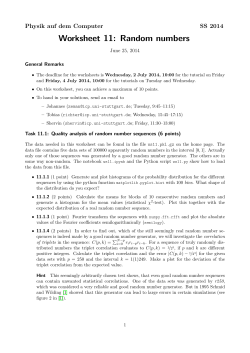


© Copyright 2026