
What is Not Taken into Account and they Did Not Notice Ampere
AASCIT Journal of Physics 2015; 1(1): 28-52 Published online March 30, 2015 (http://www.aascit.org/journal/physics) What is Not Taken into Account and they Did Not Notice Ampere, Faraday, Maxwell, Heaviside and Hertz F. F. Mende B.I. Verkin Institute for Low Temperature Physics and Engineering NAS Ukraine Email address [email protected] Citation Keywords Faraday Low, Maxwell Equations, Electromagnetic Induction, Lorentz Force, Scalar-Vector Potential, Unipolar Generator, Kinetic Inductance Received: March 8, 2015 Revised: March 21, 2015 Accepted: March 22, 2015 F. F. Mende. What is Not Taken into Account and they Did Not Notice Ampere, Faraday, Maxwell, Heaviside and Hertz. AASCIT Journal of Physics. Vol. 1, No. 1, 2015, pp. 28-52. Abstract Electrodynamics is developed already more than 200 years, in it still remained sufficiently many problems. For the duration entire of the period in the electrodynamics indicated primary attention was paid to the electrical and magnetic fields, and this concept as magnetic vector potential remained in the shadow. The carried out analysis showed that the magnetic vector potential is one of the most important concepts of classical electrodynamics, and magnetic field is only a consequence of this potential. But physical nature of this potential was not clear. The meaningful result of work is that which in them within the framework of Galilei conversions is shown that the scalar potential of charge depends on its relative speed, and this fact found its experimental confirmation. The obtained results change the ideological basis of classical electrodynamics, indicating that the substantial part of the observed in the electrodynamics dynamic phenomena, this by the consequences of this dependence. Certainly, the adoption of this concept is critical step. Indeed the main parameter of charge are those energy characteristics, which it possesses and how it influences the surrounding charges not only in the static position, but also during its motion. the dependence of scalar potential on the speed leads to the fact that in its environments are generated the electric fields, to reverse fields, that accelerate charge itself. Such dynamic properties of charge allow instead of two symmetrical laws of magneto electric and electromagnetic induction to introduce one law of electro-electrical induction, which is the fundamental law of induction. This method gives the possibility to directly solve all problems of induction and emission, without resorting to the application of such pour on mediators as vector potential and magnetic field. This approach makes it possible to explain the origin of the forces of interaction between the current carrying systems. Up to now in the classical electrodynamics existed two not connected with each other of division. From one side this of Maxwell equation, and from which follow wave equations for the electromagnetic pour on, while from other side this of the relationships, which determine power interaction of the current carrying systems. For explaining this phenomenon the postulate about the Lorentz force was introduced. Introduction to the dependence of the scalar potential of charge on the speed mutually connects these with those not connected divisions, and classical electrodynamics takes the form of the ordered united science, which has united ideological basis. 1. Introduction The basis of contemporary electrodynamics, were placed by Ampere [1], which introduced the concept of magnetic field. This made possible to obtain the mathematical relationships, which describe power interaction of the current carrying systems. But AASCIT Journal of Physics 2015; 1(1): 28-52 this task was solved only at the phenomenological level, since. The physical causes for such an interaction were not found. The following major step in the description of electrodynamic processes was conducted by Faraday [2], who introduced the law of electromagnetic induction and by Maxwell, which introduced the concept of bias current [ 3]. This made possible to predict and to describe wave processes in the material media. The meaningful result of the work of Maxwell was also the introduction of the concept of the vector potential of magnetic field, which made it possible to write down the generalized scalar potential, which unites the static and dynamic laws of electrodynamics. Heaviside's merit is the fact that he wrote down Maxwell's equations in the terms of vector analysis. Equations recorded by Heaviside and it is customary to assume Maxwell equations. However, Maxwell did not introduce the concept of the vector potential of electric field, which makes it possible to symmetrize the equations of electrodynamics, after writing down them in the plural form. The experimental detection of electromagnetic waves is the most great merit of Hertz [4]. He succeeded in creating the first in the world highfrequency generator and the antenna, capable of emitting electromagnetic waves. Lorenz is already later and Poincare introduced experimental postulate about the Lorentz force who up to now is used for enumerating the magnetic forces, which act on the charges, which move in the magnetic field. But no one of higher than enumerated scientists could explain physical nature of the vector potential of magnetic field and prove that the scalar potential of charge and its dependence on the speed is the basis of all static and dynamic laws of electrodynamics. This was made in the work of the author [5-16]. Introduction to the dependence of the scalar potential of charge from the speed not only made it possible to explain nature of the emission of electromagnetic waves, or physics of power interaction of the current carrying systems, but also combined two not connected, until now, parts of the electrodynamics, which present wave and power processes. To the examination of the role of the scalar potential of charge and its dependence on the speed to the formulating of the laws of electrodynamics is dedicated this article. The laws of classical electrodynamics they reflect experimental facts they are phenomenological. Unfortunately, contemporary classical electrodynamics is not deprived of the contradictions, which did not up to now obtain their explanation. The fundamental equations of contemporary classical electrodynamics are the Maxwell equation. They are written as follows for the vacuum: ∂B , ∂t (1.1) ∂D , ∂t (1.2) rot E = − rot H = 29 div D = 0 , (1.3) div B = 0 , (1.4) where E , H are tension of electrical and magnetic field, D = ε 0 E , B = µ0 H are electrical and magnetic induction, µ0 , ε 0 are magnetic and dielectric constant of vacuum. From Maxwell equations follow the wave equations ∇ 2 E = µ0ε 0 ∂2 E , ∂t 2 (1.5) ∇ 2 H = µ0 ε 0 ∂2 H . ∂t 2 (1.6) These equations show that in the vacuum can be extended the plane electromagnetic waves, the velocity of propagation of which is equal to the speed of light c= 1 µ 0ε 0 . (1.7) For the material media the Maxwell equations take the following form: ɶ 0 rot E = − µµ ɶ 0 rot H = nev + εε ∂H ∂B , =− ∂t ∂t (1.8) ∂E ∂D , = nev + ∂t ∂t (1.9) div D = ne , (1.10) div B = 0 , (1.11) where µɶ , εɶ are the relative magnetic and dielectric constants of the medium and n , e and v are density, value and charge rate. The equations (1.1 - 1.11) are written in the assigned inertial reference frame (IRF) and in them there are no rules of passage of one IRF to another. These equations assume that the properties of charge do not depend on their speed. In Maxwell equations are not contained indication that is the reason for power interaction of the current-carrying systems, therefore to be introduced the experimental postulate about the force, which acts on the moving charge in the magnetic field FL = e v × µ0 H . (1.12) This force is called the Lorentz force. However in this axiomatics is an essential deficiency. If force acts on the moving charge, then in accordance with third Newton law must occur and reacting force. In this case the magnetic field is independent substance, comes out in the role of the 30 F. F. Mende: What is Not Taken into Account and they Did Not Notice Ampere, Faraday, Maxwell, Heaviside and Hertz mediator between the moving charges. Consequently, we do not have law of direct action, which would give immediately answer to the presented question, passing the procedure examined. I.e. we cannot give answer to the question, where are located the forces, the compensating action of magnetic field to the charge. The equation (1.12) from the physical point sight causes bewilderment. The forces, which act on the body in the absence of losses, must be connected either with its acceleration, if it accomplishes forward motion, or with the centrifugal forces, if body accomplishes rotary motion. Finally, static forces appear when there is the gradient of the scalar potential of potential field, in which is located the body. But in Eq. (1.12) there are no such forces. Usual rectilinear motion causes the force, which is normal to the direction motion. In the classical mechanics the forces of this type are unknown. Is certain, magnetic field is one of the important concepts of contemporary electrodynamics. Its concept consists in the fact that around any moving charge appears the magnetic field (Ampere law), whose circulation is determined by equation ∫ Hdl = I , (1.13) where I is conduction current. Equation (1.9) is the consequence of Eq. (1.13), if we to the conduction current add bias current. Let us especially note that the introduction of the concept of magnetic field does not be founded upon any physical basis, but it is the statement of the collection of some experimental facts. Using this concept, it is possible with the aid of the specific mathematical procedures to obtain correct answer with the solution of practical problems. But, unfortunately, there is a number of the physical questions, during solution of which within the framework the concepts of magnetic field, are obtained paradoxical results. Here one of them. Using Eqs. (1.12) and (1.13) not difficult to show that with the unidirectional parallel motion of two like charges, or flows of charges, between them must appear the additional attraction. However, if we pass into the inertial system, which moves together with the charges, then there magnetic field is absent, and there is no additional attraction. This paradox does not have an explanation. Of force with power interaction of material structures, along which flows the current, are applied not only to the moving charges, but to the lattice, but in the concept of magnetic field to this question there is no answer also, since. In Eqs. (1.1-1.13) the presence of lattice is not considered. At the same time, when current flows through the plasma, occurs its compression. This phenomenon is called pinch effect. In this case forces of compression act not only on the moving electrons, but also on the positively charged ions. And, again, the concept of magnetic field cannot explain this fact, since in this concept there are no forces, which can act on the ions of plasma. As the fundamental law of induction in the electrodynamics is considered Faraday law, consequence of whom is the Maxwell first equation. However, here are problems. It is considered until now that the unipolar generator is an exception to the rule of flow, consequently Faraday law is not complete. Let us give one additional statement of the monograph [17]: “The observations of Faraday led to the discovery of new law about the connection of electrical and magnetic field on: in the field, where magnetic field changes in the course of time, is generated electric field”. But from this law also there is an exception. Actually, the magnetic fields be absent out of the long solenoid; however, electric fields are generated with a change of the current in this solenoid around the solenoid. In the classical electrodynamics does not find its explanation this well known physical phenomenon, as phase aberration of light. From entire aforesaid it is possible to conclude that in the classical electrodynamics there is number of the problems, which still await their solution. 2. Laws of the Magnetoelectric Induction The primary task of induction is the presence of laws governing the appearance of electrical field on, since only electric fields exert power influences on the charge. Faraday law is written as follows: ∫ E dl =− ∂ФB ∂H ∂B = −µ ∫ ds = −∫ ds , ∂t ∂t ∂t (2.1) where B = µ H is magnetic induction vector, ФB = µ ∫ H ds ɶ 0 is magnetic is flow of magnetic induction, and µ = µµ permeability of medium. It follows from this law that the circulation integral of the vector of electric field is equal to a change in the flow of magnetic induction through the area, which this outline covers. From Eq.(2.1) obtain the Maxwell first equation rot E = − ∂B . ∂t (2.2) Let us immediately point out to the terminological error. Faraday law should be called not the law of electromagnetic, as is customary in the existing literature, but by the law of magneto electric induction, since. a change in the magnetic field on it leads to the appearance of electrical field on, but not vice versa. Let us introduce the vector potential of the magnetic field AH , which satisfies the equality µ ∫ AH dl = ФB , where the outline of the integration coincides with the outline of integration in Eq. (2.1), and the vector of is determined in AASCIT Journal of Physics 2015; 1(1): 28-52 all sections of this outline, then then E = −µ ∂AH . ∂t (2.3) Between the vector potential and the electric field there is a local connection. Vector potential is connected with the magnetic field with the following equation: rot AH = H . (2.4) During the motion in the three-dimensional changing field of vector potential the electric fields find, using total derivative E ′ = −µ dAH . dt (2.5) Prime near the vector E means that we determine this field in the moving coordinate system. This means that the vector potential has not only local, but also convection derivative. In this case Eq. (2.5) can be rewritten as follows: E ′ = −µ ∂AH − µ ( v ∇ ) AH , ∂t of this potential. Entirely different nature in force, which is determined by last term Eq. (2.6). It is connected with the fact that the charge, which moves in the field of vector potential, it possesses potential energy, whose gradient gives force. From Eq. (2.6) follows E ′ = −µ (2.7) ( ) µ grad vAH − µ ( v ∇ ) AH = µ v × rot AH , Fv′ = eµ v × rot AH , This force depends only on the gradients of vector potential and charge rate. The charge, which moves in the field of the vector potential AH with the speed v , possesses potential energy ( ) W = −eµ vAH . (2.8) and, taking into account (2.4), let us write down Fv′ = e µ v × H (2.9) Ev′ = µ v × H , (2.10) or Therefore must exist one additional force, which acts on the charge in the moving coordinate system, namely: ( ) Fv′,2 = − grad W = eµ grad vAH . plays the same role, as the scalar ∂AH − eµ ( v ∇ ) AH + eµ grad vAH . ∂t ( ) and it is final F ′ = eE + eEv′ = −e potential of the charge, whose gradient determines the force, which acts on the moving charge. Consequently, the composite force, which acts on the charge, which moves in the field of vector potential, can have three components and will be written down as F ′ = −eµ ( ) that from Eq. (2.6) we will obtain Fv′,1 = − µ e ( v ∇ ) AH . ( ) ∂AH − µ ( v ∇ ) AH + µ grad vAH . ∂t This is a complete law of mutual induction. It defines all electric fields, which can appear at the assigned point of space, this point can be both the fixed and that moving. This united law includes and Faraday law and that part of the Lorentz force, which is connected with the motion of charge in the magnetic field, and without any exceptions gives answer to all questions, which are concerned mutual magnetoelectric induction. It is significant, that, if we take rotor from both parts of equality (2.7), attempting to obtain the Maxwell first equation, then it will be immediately lost the essential part of the information, since. rotor from the gradient is identically equal to zero. If we isolate those forces, which are connected with the motion of charge in the three-dimensional changing field of vector potential, and to consider that where v is speed of system. If vector potential on time does not depend, the force acts on the charge The value eµ vAH 31 (2.6) The first of the components of this force acts on the fixed charge, when vector potential changes in the time and has local time derivative. Second component is connected with the motion of charge in the three-dimensional changing field ∂AH + eµ v × H . ∂t (2.11) Can seem that Eq. (2.11) presents Lorentz force, however, this not thus. In this equation, in contrast to the Lorentz force the field E is induction. In order to obtain the total force, which acts on the charge, necessary to the right side Eq. (2.11) to add the term −e grad ϕ F∑′ = −e grad ϕ + eE + eµ v × H , where ϕ is scalar potential at the observation point. In this case Eq.(2.7) can be rewritten as follows: 32 F. F. Mende: What is Not Taken into Account and they Did Not Notice Ampere, Faraday, Maxwell, Heaviside and Hertz E ′ = −µ ∂AH − µ ( v ∇ ) AH + µ grad vAH − grad ϕ ∂t ( ) (2.12) or E ′ = −µ ( ( ) ) dAH + grad µ vA − ϕ . dt (2.13) If both parts of Eq. (2.12) are multiplied by the magnitude of the charge, then will come out the total force, which acts on the charge. From Lorentz force it will differ in terms of the force −eµ ( ) ∂AH .From Eq. (2.13) it is evident that the value ∂t µ vA − ϕ plays the role of the generalized scalar potential. After taking rotor from both parts of Eq. (2.13) and taking into account that rot grad = 0 , we will obtain rot E ′ = − µ dH . dt d ΦB . dt moves in the three-dimensional changing field B . The value of magnetic flux in Eq. (2.14) is determined from the equation ФB = ∫ Bds ′ (2.15) where the magnetic induction B = µ H is determined in the fixed IRF, and the element ds′ is determined in the moving system. Taking into account Eq. (2.14), from Eq. (2.15) we obtain d If we in this equation replace total derivative by the quotient, then we will obtain the Maxwell first equation. After performing this operation, we obtained the Maxwell first equation, but they lost information about power interaction of the moving charge with the magnetic field. This examination maximally explained the physical picture of mutual induction. We specially looked to this question from another point of view, in order to permit those contradictory judgments, which occur in the fundamental monograph according to the theory of electricity. Previously Lorentz force was considered as the fundamental experimental postulate, not connected with the law of induction. By calculation to obtain last term of the right side of Eq. (2.11) was only within the framework special relativity (SP), after introducing two postulates of this theory. In this case all terms of Eq. (2.11) are obtained from the law of induction, using the Galileo conversions. Moreover Eq. (2.11) this is a complete law of mutual induction, if it are written down in the terms of vector potential. And this is the very thing rule, which gives possibility, knowing fields in one IRF, to calculate fields in another. With conducting of experiments Faraday established that in the outline is induced the current, when in the adjacent outline direct current is switched on or is turned off or adjacent outline with the direct current moves relative to the first outline. Therefore in general form Faraday law is written as follows: ∫ E′dl ′ = − E and dl be absent, but in this case to the right in expression (2.14) must stand particular time derivative. Complete time derivative in Eq. (2.14) indicates the independence of the eventual result of appearance e.m.f. in the outline from the method of changing the flow. Flow can change both due to the change of B with time and because the system, in which is measured the circulation ∫ E ′dl ′ , it ∫ E ′dl ′ = − dt ∫ B ds′ . and further, since ∂B ∫ E ′dl ′ = − ∫ ∂t ds ′ − ∫ B × v dl ′ − ∫ vdivBds′ . (2.16) In this case contour integral is taken on the outline dl ′ , which covers the area ds′ . Let us immediately note that entire following presentation will be conducted under the assumption the validity of the Galileo conversions, i.e., dl ′ = dl and ds ′ = ds . From (2.16) follows the known result E ′ = E + v × B , (2.17) from which follows that during the motion in the magnetic field the additional electric field, determined by last term of equation appears (2.17). Let us note that this equation is obtained not by the introduction of postulate about the Lorentz force, or from the Lorenz conversions, but directly from the Faraday law, moreover within the framework the conversions of Galileo. Thus, Lorentz force is the direct consequence of the law of magnetoelectric induction. The equation follows from the Ampere law H = rot AH . Then Eq. (2.16) can be rewritten (2.14) This writing of law indicates that with the determination of the circulation E in the moving IRF, near E and dl must stand primes and should be taken total derivative. But if circulation is determined in the fixed IRF, then primes near d ∂ = + v grad , let us write down dt ∂t E′ = −µ ∂AH + µ v × rotA , ∂t and further E ′ = −µ ∂AH − µ ( v ∇ ) AH + µ grad vAH . ∂t ( ) (2.18) AASCIT Journal of Physics 2015; 1(1): 28-52 Again came out Eq. (2.7), but it is obtained directly from the Faraday law. True, and this way thus far not shedding light on physical nature of the origin of Lorentz force, since the true physical causes for appearance and magnetic field and vector potential to us nevertheless are not thus far clear. With the examination of the forces, which act on the charge, we limited to the case, when the time lag, necessary for the passage of signal from the source, which generates vector potential, to the charge itself was considerably less than the period of current variations in the conductors. Now let us remove this limitation. The Maxwell second equationin the terms of vector potential can be written down as follows: ( ) rot rotAH = j AH , (2.19) where j ( AH ) is certain functional from AH , depending on the properties of the medium in question. If is carried out Ohm law j = σ E , then j ( AH ) = −σµ ∂AH . ∂t (2.20) 33 vector potential can be extended in the free space in the form of plane waves, and it on its information capability does not be inferior to the wave equations, obtained from Maxwell's equations. This equation on its information capability does not be inferior to wave equations for the electrical and magnetic field on, obtained from Maxwell equations. Everything said attests to the fact that in the classical electrodynamics the vector potential has important significance. Its use shedding light on many physical phenomena, which previously were not intelligible. And, if it will be possible to explain physical nature of this potential, then is solved the very important problem both of theoretical and applied nature. 3. Laws of the Electromagnetic Induction The Faraday law shows, how a change in the magnetic field on it leads to the appearance of electrical field on. However, does arise the question about that, it does bring a change in the electrical field on to the appearance of magnetic field on? In the case of the absence of conduction currents the the Maxwell second equation appears as follows: For the free space takes the form: j ( AH ) = − µε ∂ AH . ∂t 2 rot H = ε 2 (2.21) ∂E ∂D , = ∂t ∂t where D = ε E is electrical induction. And further For the free charges the functional takes the form: of j ( AH ) = − µ Lk AH , ∫ H dl (2.22) ∂Φ E , ∂t (3.1) where Φ E = ∫ Dds is the flow of electrical induction. m where Lk = 2 is kinetic inductance of charges [18,19]. In ne this equation m is the mass of charge, e is the magnitude of the charge, n is charge density. Equations (2.20 - 2.22) reflect well-known fact about existence of three forms of the electric current: active and two reactive. Each of them has characteristic dependence on the vector potential. This dependence determines the rules of the propagation of vector potential in different media. Here one should emphasize that Eqs. (2.20 - 2.22) assume not only the presence of current, but also the presence of those material media, in which such currents can leak. The conduction current, determined by Eqs. (2.20) and (2.22), can the leak through the conductors, in which there are free current carriers. Bias current, can the leak through the free space or the dielectrics. For the free space Eq. (2.19) takes the form: rot rotAH = − µε = ∂ AH . ∂t 2 2 (2.23) This wave equation, which attests to the fact that the However for the complete description of the processes of the mutual electrical induction of Eq. (3.1) is insufficient. As in the case Faraday law, should be considered the circumstance that the flow of electrical induction can change not only due to the local derivative of electric field on the time, but also because the outline, along which is produced the integration, it can move in the three-dimensional changing electric field. This means that in Eq. (3.1), as in the case Faraday law, should be replaced the partial derivative by the complete. Designating by the primes of field and circuit elements in moving IRF, we will obtain: ∫ H ′dl ′ = d ΦE , dt and further ∂D ∫ H ′dl ′ = ∫ ∂t ds ′ + ∫ D × v dl ′ + ∫ vdivDds′ . (3.2) For the electrically neutral medium divE = 0 , therefore the last member of right side in this expression will be absent. For this case Eq. (3.2) will take the form: 34 F. F. Mende: What is Not Taken into Account and they Did Not Notice Ampere, Faraday, Maxwell, Heaviside and Hertz ∂D ∫ H ′dl ′ = ∫ ∂t ds′ + ∫ D × v dl ′ . (3.3) If we in this equation pass from the contour integration to the integration for the surface, then we will obtain: rotH ′ = ∂D + rot D × v . ∂t H = rot AH , (4.1) E = rot AE . (4.2) Consequently, Maxwell equations can be written down with the aid of these potentials: E = rot AE . (3.6) Equation (3.4) taking into account Eq.(3.6) will be written down: ∂AE − ε v × rot AE . ∂t Further it is possible to repeat all those procedures, which has already been conducted with the magnetic vector potential, and to write down the following equations: ∂AE + ε ( v ∇ ) AE − ε grad vAE , ∂t ( ) ∂A H ′ = ε E − ε v × rot AE , ∂t dAE − ε grad ( vAE ) . dt Is certain, the study of this problem it would be possible, as in the case the law of magnetoelectric induction, to begin from the introduction of the vector AE . This procedure was for the first time proposed in article [5]. The introduction of total derivatives in the laws of induction substantially explains physics of these processes and gives the possibility to isolate the force components, which act on the charge. This method gives also the possibility to obtain transformation laws fields on upon ∂AH ∂t (4.3) ∂AE . ∂t (4.4) rot AE = −µ (3.5) It is possible to express the electric field through the rotor of electrical vector potential, after assuming H′ = ε In the previous paragraph it is shown that the magnetic and electric fields can be expressed through their vector potentials rot AH = ε H v′ = −ε v × E . H′ = ε 4. Plurality of the Forms of the Writing of the Electrodynamic Laws (3.4) If we, based on this equation, write down fields in this inertial system, then prime near H and second member of right side will disappear, and we will obtain the bias current, introduced by Maxwell. But Maxwell introduced this parameter, without resorting to the law of electromagnetic induction. If his law of magnetoelectric induction Faraday derived on the basis experiments with the magnetic fields, then experiments on the establishment of the validity of Eq. (3.2) cannot be at that time conducted was, since for conducting this experiment sensitivity of existing at that time meters did not be sufficient. On from Eq.(3.4) we obtain for the case of constant electrical field: H′ = ε transfer of one IRF to another. For each of these potentials it is possible to obtain wave equation, in particular rot rot AE = −εµ ∂ 2 AE ∂t 2 (4.5) and to consider that in the space are extended not the magnetic and electric fields, but the field of electrical vector potential. In this case, as can easily be seen of the Eqs. (4.1 - 4.4), magnetic and electric field they will be determined through this potential by the equations: ∂AE ∂t . E = rot AE H =ε Space derivative rot AE and local time derivative (4.6) ∂AE are ∂t connected with wave equation (4.5). Thus, the use only of one electrical vector potential makes it possible to completely solve the task about the propagation of electrical and magnetic field on. Taking into account (4.6), Pointing vector can be written down only through the vector AE : ∂A P = ε E × rot AE . ∂ t Characteristic is the fact that with this method of examination necessary condition is the presence at the particular point of space both the time derivatives, and space derivative of one and the same potential. AASCIT Journal of Physics 2015; 1(1): 28-52 This task can be solved by another method, after writing down wave equation for the magnetic vector potential: rot rot AH = −εµ ∂ 2 AH . ∂t 2 (4.7) In this case magnetic and electric fields will be determined by the equations: H = rot AH E = −µ ∂AH . ∂t Pointing vector in this case can be found from the following equation: ∂A P = − µ H × rot AH ∂t . Space derivative rot AH and local time derivative of ∂AH ∂t are connected with wave equation (4.7). But it is possible to enter and differently, after introducing, for example, the electrical and magnetic currents jE = rot H , jH = rot E . The equations also can be recorded for these currents: rot jH = − µ rot jE = ε ∂j E , ∂t ∂j H . ∂t This system in its form and information concluded in it differs in no way from Maxwell equations, and it is possible to consider that in the space the magnetic or electric currents are extended. And the solution of the problem of propagation with the aid of this method will again include complete information about the processes of propagation. The method of the introduction of new vector examined field on it is possible to extend into both sides ad infinitum, introducing all new vectorial fields. Naturally in this case should be introduced additional calibrations. Thus, there is an infinite set of possible writings of electrodynamic laws, but they all are equivalent according to the information concluded in them. This approach was for the first time demonstrated in the article [5]. derivatives field on and vector potential it was begun still in Maxwell, since it wrote its equations in the total derivatives. Hertz also wrote the equations of electrodynamics in the total derivatives. Hertz did not introduce the concept of vector potentials, but he operated only with fields, but this does not diminish its merits. It made mistakes only in the fact that the electrical and magnetic fields were considered the invariants of speed. But already simple example of long lines is evidence of the inaccuracy of this approach. With the propagation of wave in the long line it is filled up with two forms of energy, which can be determined through the currents and the voltages or through the electrical and magnetic fields in the line. And only after wave will fill with electromagnetic energy all space between the generator and the load on it will begin to be separated energy. I.e. the time, by which stays this process, generator expended its power to the filling with energy of the section of line between the generator and the load. But if we begin to move away load from incoming line, then a quantity of energy being isolated on it will decrease, since. the part of the energy, expended by source, will leave to the filling with energy of the additional length of line, connected with the motion of load. If load will approach a source, then it will obtain an additional quantity of energy due to the decrease of its length. But if effective resistance is the load of line, then an increase or the decrease of the power expendable in it can be connected only with a change in the stress on this resistance. Being located in assigned IRF, us interest those fields, which are created in it by the fixed and moving charges, and also by the electromagnetic waves, which are generated by the fixed and moving sources of such waves. The fields, which are created in this IRF by moving charges and moving sources of electromagnetic waves, we will call dynamic. Can serve as an example of dynamic field the magnetic field, which appears around the moving charges. As already mentioned, in the classical electrodynamics be absent the rule of the conversion of electrical and magnetic field on upon transfer of one inertial system to another. This deficiency removes SR, basis of which are the Lorenz conversions. With the entire mathematical validity of this approach the physical essence of such conversions up to now remains unexplained. in this division will made attempt find the precisely physically substantiated ways of obtaining the conversions field on upon transfer of one IRF to another, and to also explain what dynamic potentials and fields can generate the moving charges. The first step in this direction was made a way of the introduction of the symmetrical laws of magnetoelectric and electromagnetic induction [5]. These laws are written as follows: ∂B ∫ E ′dl ′ = −∫ ∂t ds + ∫ v × B dl ′ 5. Dynamic Potentials and the Field of the Moving Charges The way, which is concerned the introduction of total 35 ∂D ∫ H ′dl ′ =∫ ∂t ds − or ∫ v × D dl ′ (5.1) 36 F. F. Mende: What is Not Taken into Account and they Did Not Notice Ampere, Faraday, Maxwell, Heaviside and Hertz ∂B + rot v × B ∂t . ∂D rotH ′ = − rot v × D dt rotE ′ = − (5.2) where v ⊥ is normal component of charge rate to the vector, which connects the moving charge and observation point. Expression for the scalar potential, created by the moving charge, for this case will be written down as follows: v⊥ c = ϕ (r )ch v⊥ ϕ ′(r , v⊥ ) = 4πε r c For the constants fields on these equations they take the form: E ′ = v × B H ′ = − v × D . (5.3) In Eqs. (5.1-5.3), which assume the validity of the Galileo conversions present fields and elements in moving and fixed IRF respectively. It must be noted, that conversions (5.3) earlier could be obtained only from the Lorenz conversions. Equations (5.1-5.3), which present the laws of induction, do not give information about how arose fields in initial fixed IRF. They describe only laws governing the propagation and conversion fields on in the case of motion with respect to the already existing fields. Equation(5.3) attest to the fact that in the case of relative motion of frame of references, between the fields E and H there is a cross coupling, i.e., motion in the fields H leads to the appearance field on E and vice versa. From these equations escape the additional consequences. g The electric field E = beyond the limits of the 2πε r charged long rod, where g is a linear charge, diminishes 1 according to the law . r If we in parallel to the axis of rod in the field E begin to move with the speed ∆v another IRF, then in it will appear the additional magnetic field ∆H = ε E ∆v . If we now with respect to already moving IRF begin to move third frame of reference with the speed ∆v , then already due to the motion in the field ∆H will appear additive to the electric field 2 ∆E = µε E ( ∆ v ) . This process can be continued and further, as a result of which can be obtained the number, which gives the value of the electric field Ev′ ( r ) in moving IRF with reaching of the speed v = n∆v , when ∆v → 0 , and n → ∞ .In the final analysis in moving IRF the value of dynamic electric field will prove to be more than in the initial and to be determined by the equation: v⊥ c = Ech v⊥ . E ′ ( r , v⊥ ) = 2πε r c gch If speech goes about the electric field of the single charge e , then its electric field will be determined by the equation: v⊥ c , E ′ ( r , v⊥ ) = 4πε r 2 ech ech (5.4) where ϕ ( r ) is scalar potential of fixed charge. The potential ϕ ′(r , v⊥ ) can be named scalar-vector, since it depends not only on the absolute value of charge, but also on speed and direction of its motion with respect to the observation point. Maximum value this potential has in the direction normal to the motion of charge itself. Moreover, if charge rate changes, which is connected with its acceleration, then can be calculated the electric fields, induced by the accelerated charge. During the motion in the magnetic field, using the already examined method, we obtain: H ′(v⊥ ) = Hch v⊥ . c where v ⊥ isspeed normal to the direction of the magnetic field. If we apply the obtained results to the electromagnetic wave and to designate components fields on parallel speeds IRF as E↑ , H ↑ , and E⊥ , H ⊥ as components normal to it, then conversions fields on they will be written down: E↑′ = E↑ , v Z v E⊥′ = E⊥ ch + 0 v × H ⊥ sh , c v c H ↑′ = H ↑ , (5.5) v 1 v v × E⊥ sh , H ⊥′ = H ⊥ ch − c c vZ 0 where Z 0 = µ0 is impedance of free space, c = ε0 1 µ 0ε 0 is speed of light. Conversions fields on (5.5) they were for the first time obtained in the article [5]. 6. Phase Aberration and the Transverse Doppler Effect Using Eqs. (5.5) it is possible to explain the phenomenon of phase aberration, which did not have within the framework existing classical electrodynamics of explanations. We will consider that there are components of the plane wave H z , E x , which is extended in the direction y , and primed system moves in the direction of the axis x with the speed v x . Then components fields will be written down: AASCIT Journal of Physics 2015; 1(1): 28-52 Ex′ = Ex , vx , c v H z′ = H z ch x . c E y′ = H z sh Thus is a heterogeneous wave, which has in the direction of propagation the component Ev′ . Let us write down the summary field E ′ in moving IRF 1 2 2 v 2 E ′ = ( Ex′ ) + ( E y′ ) = Ex ch x . c (6.1) If the vector H ′ is as before orthogonal the axis y , then the vector E ′ is now inclined toward it to the angle α , determined by the equation: v c v c α ≅ sh ≅ . (6.2) Thisis phase aberration. Specifically, to this angle to be necessary to incline telescope in the direction of the motion of the Earth around the sun in order to observe stars, which are located in the zenith. The Poynting vector is now also directed no longer along the axis y , but being located in the plane xy , it is inclined toward the axis y to the angle, determined by Eqs. (6.2). However, the relation of the absolute values of the vectors of E ′ and H ′ in both systems they remained identical. However, the absolute value of Poynting vector increased. Thus, even transverse motion of inertial system with respect to the direction of propagation of wave increases its energy in the moving system. This phenomenon is understandable from a physical point of view. It is possible to give an example with the rain drops. When they fall vertically, then is energy in them one. But in the inertial system, which is moved normal to the vector of their of speed, to this speed the velocity vector of inertial system is added. In this case the absolute value of the speed of drops in the inertial system will be equal to square root of the sum of the squares of the speeds indicated. The same result gives to us Eq. (6.1). Such waves have in the direction of its propagation additional of the vector of electrical or magnetic field, and in this they are similar to E and H of the waves, which are extended in the waveguides. In this case appears the uncommon wave, whose phase front is inclined toward the Poynting vector to the angle, determined by Eq. (10.2). In fact obtained wave is the superposition of plane wave with the phase speed c = 1 µε and additional wave of plane wave with the infinite phase speed orthogonal to the direction of propagation. The transverse Doppler effect, who long ago is discussed sufficiently, until now, did not find its confident experimental confirmation. For observing the star from moving IRF it is 37 necessary to incline telescope on the motion of motion to the angle, determined by Eq. (6.2). But in this case the star, observed with the aid of the telescope in the zenith, will be in actuality located several behind the visible position with respect to the direction of motion. Its angular displacement from the visible position in this case will be determined by Eq. (6.2). But this means that this star with respect to the observer has radial speed, determined by the equation vr = v sin α . Since for the low values of the angles sin α ≅ α , and v α = , Doppler frequency shift will compose c ωd ⊥ = ω0 v2 . c2 (6.3) This result numerically coincides with results SR, but it is principally characterized by of results. It is considered SR that the transverse Doppler effect, determined by Eq. (6.3), there is in reality, while in this case this only apparent effect. If we compare the results of conversions fields on (6.5) with conversions SP, then it is not difficult to see that they coincide with an accuracy to the quadratic members of the ratio of the velocity of the motion of charge to the speed of light. Conversion SP, although they were based on the postulates, could correctly explain sufficiently accurately many physical phenomena, which before this explanation did not have. With this circumstance is connected this great success of this theory. Conversions (6.4) and (6.5) are obtained on the physical basis without the use of postulates and they with the high accuracy coincided with SP. Difference is the fact that in conversions (6.5) there are no limitations on the speed for the material particles, and also the fact that the charge is not the invariant of speed. The experimental confirmation of the fact indicated can serve as the confirmation of correctness of the proposed conversions. 7. The Problem of the Lorentz Force and Power Interaction of the Current-Carrying Systems and Its Solution It was already said, that Maxwell equations do not include information about power interaction of the current carrying systems. In the classical electrodynamics for calculating such an interaction it is necessary to calculate magnetic field in the assigned region of space, and then, using a Lorentz force, to find the forces, which act on the moving charges. Obscure a question about that remains with this approach, to what are applied the reacting forces with respect to those forces, which act on the moving charges. The concept of magnetic field arose to a considerable degree because of the observations of power interaction of 38 F. F. Mende: What is Not Taken into Account and they Did Not Notice Ampere, Faraday, Maxwell, Heaviside and Hertz the current carrying and magnetized systems. Experience with the iron shavings, which are erected near the magnet poles or around the annular turn with the current into the clear geometric figures, is especially significant. These figures served as occasion for the introduction of this concept as the lines of force of magnetic field. In accordance with third Newton law with any power interaction there is always a equality of effective forces and opposition, and also always there are those elements of the system, to which these forces are applied. A large drawback in the concept of magnetic field is the fact that it does not give answer to that, counteracting forces are concretely applied to what, since. magnetic field comes out as the independent substance, with which occurs interaction of the moving charges. Is experimentally known that the forces of interaction in the current carrying systems are applied to those conductors, whose moving charges create magnetic field.However, in the existing concept of power interaction of such systems the positively charged lattice, to which are applied the forces, does not participate in the formation of the forces of interaction. Let us examine this question on the basis of the concept of scalar- vector potential. We will consider that the scalarvector potential of single charge is determined by Eq. (9.4), and that the electric fields, created by this potential, act on all surrounding charges, including to the charges positively charged lattices. Let us examine from these positions power interaction between two parallel conductors (Fig. 1), along which flow the currents. We will consider that g1+ , g 2 + and g1− , g 2 − present the respectively fixed and moving linear charges. search for as the sum of four forces, whose designation is understandable from the figure. The repulsive forces F1 , F2 we will take with the minus sign, while the attracting force F3 , F4 we will take with the plus sign. For the single section of the two-wire circuit of force, acting between the separate subsystems, will be written down g1+ g 2 + , 2πε r g −g − v −v F2 = − 1 2 ch 1 2 , 2πε r c g1− g 2 + v1 F3 = + ch , 2πε r c g1+ g 2 − v2 F4 = + ch . 2πε r c F1 = − (7.1) Adding all force components, we will obtain the amount of the composite linearforce FΣ = g1 g 2 v1 v v −v ch + ch 2 − ch 1 2 − 1 . 2πε r c c c (7.2) In this expression as g1 and g 2 are undertaken the absolute values of the linearcharges, and the signs of forces are taken into account in the bracketed expression.For the case v ≪ c let us take only two first members of expansion v in the series ch , i.e., we will consider that c v 1 v2 ch ≅ 1 + .From Eq. (7.2) we obtain 2 c2 c g1v1 g 2 v2 II = 1 22 2 2πε c r 2πε c r FΣ1 = (7.3) where as g1 and g 2 are undertaken the absolute values of the linear charges, and v1 , v2 take with its signs. Since the magnetic field of straight wire, along which flows the current I , we determine by the equation H= Fig. 1. Schematic of power interaction of the current carrying wires of twowire circuit taking into account the positively charged lattice. The linearcharges g1+ , g 2 + present the positively charged lattice in the lower and upper conductors. We will also consider that both conductors prior to the start of charges are electrically neutral. This means that in the conductors are two systems of the mutually inserted opposite charges with the lineardensity g1+ , g1− and g 2 + , g 2 − , which neutralize each other.In Fig. 1 these systems for larger convenience in the examination of the forces of interaction are moved apart along the axis z . Subsystems with the negative charge (electrons) can move with the speeds v1 , v2 . The force of interaction between the lower and upper conductors we will I , 2π r from Eq. (7.3) we obtain FΣ1 = I1 I 2 HI = 1 22 = I 2 µ H1 , 2 2πε c r ε c where H1 is the magnetic field, created by lower conductor in the location of upper conductor. It is analogous FΣ1 = I1 µ H 2 , where H 2 is the magnetic field, created by upper conductor in the region of the arrangement of lower conductor. These equations coincide with the results, obtained on the AASCIT Journal of Physics 2015; 1(1): 28-52 basis of the concept of magnetic field and Lorentz forces. Equation (7.3) represents the known rule of power interaction of the current-carrying systems, but it is obtained not on the basis the introduction of phenomenological magnetic field, but on the basis of completely intelligible physical procedures. In the formation of the forces of interaction in this case the lattice takes direct part, which is not in the model of magnetic field. In the model examined are well visible the places of application of force. The obtained equations coincide with the results, obtained on the basis of the concept of magnetic field and by the axiomatically introduced Lorentz force. In this case is undertaken only first member of expansion in the series v ch .For the speeds v ≈ c should be taken all terms of c expansion. If we consider this circumstance, then the connection between the forces of interaction and the charge rates proves to be nonlinear. This, in particular it leads to the fact that the law of power interaction of the current-carrying systems is asymmetric. With the identical values of currents, but with their different directions, the attracting forces and repulsion become unequal. Repulsive forces prove to be greater than attracting force. This difference is small and is determined by the expression ∆F = v 2 I1 I 2 , 2c 2 2πε c 2ε g1 g 2 v2 v −v ch − ch 1 2 2πε r c c FΣ = g1 g 2 v1v2 1 v12 − 2πε r c 2 2 c 2 . (7.5) From Eq. (7.5) follows that with the unidirectional electron motion in the conductor and in the electronic flux the force of 1 interaction with the fulfillment of conditions v1 = v2 is 2 absent. Since the speed of the electronic flux usually much higher than speed of current carriers in the conductor, the second term in the brackets in Eq. (7.5) can be disregarded. Then, since H1 = g1v1 2πε c 2 r we will obtain the magnetic field, created by lower conductor in the place of the motion of electronic flux: FΣ = g1 g 2 v1v2 = g 2 µ v2 H . 2πε r c 2 In this case, the obtained value of force coincides with the value of Lorentz force. Taking into account that FΣ = g 2 E = g 2 µ v2 H , but with the speeds of the charge carriers of close ones to the speed of light it can prove to be completely perceptible. Let us remove the lattice of upper conductor, after leaving only free electronic flux. In this case will disappear the forces F1 , F3 , and this will indicate interaction of lower conductor with the flow of the free electrons, which move with the speed v2 on the spot of the arrangement of upper conductor. In this case the value of the force of interaction is defined as: FΣ = 39 . (7.4) Lorentz force assumes linear dependence between the force, which acts on the charge, which moves in the magnetic field, and his speed. However, in the obtained equation the dependence of the amount of force from the speed of electronic flux will be nonlinear. From Eq. (7.4) see that with an increase in v2 the deviation from the linear law increases, and in the case, when v2 ≫ v1 , the force of interaction are approached zero. This is meaningful result. Specifically, this phenomenon observed in their known experiments Thompson and Kauffmann, when they noted that with an increase in the velocity of electron beam it is more badly slanted by magnetic field. They connected the results of their observations with an increase in the mass of electron. As we see reason here another. Let us note still one interesting result. From Eq. (7.3) the force of interaction of electronic flux with a straight wire to determine according to the following dependence: it is possible to consider that on the charge, which moves in the magnetic field, acts the electric field E , directed normal to the direction of the motion of charge. This result also with v2 an accuracy to of the quadratic terms 2 completely c coincides with the results of the concept of magnetic field and is determined Lorentz force. As was already said, one of the important contradictions to the concept of magnetic field is the fact that two parallel beams of the like charges, which are moved with the identical speed in one direction, must be attracted. In this model there is no this contradiction already. If we consider that the charge rates in the upper and lower wire will be equal, and lattice is absent, i.e., to leave only electronic fluxes, then will remain only the repulsive force F2 . Thus, the moving electronic flux interacts simultaneously both with the moving electrons in the lower wire and with its lattice, and the sum of these forces of interaction it is called Lorentz force. Regularly does appear a question, and does create magnetic field most moving electron stream of in the absence compensating charges of lattice or positive ions in the plasma? The diagram examined shows that the effect of power interaction between the current carrying systems requires in the required order of the presence of the positively charged lattice. Therefore most moving electronic flux cannot create that effect, which is created during its motion in the positively charged lattice. Let us demonstrate still one approach to the problem of 40 F. F. Mende: What is Not Taken into Account and they Did Not Notice Ampere, Faraday, Maxwell, Heaviside and Hertz power interaction of the current carrying systems. The statement of facts of the presence of forces between the current carrying systems indicates that there is some field of the scalar potential, whose gradient ensures the force indicated. But that this for the field? Equation (7.3) gives only the value of force, but he does not speak about that, the gradient of what scalar potential ensures these forces. We will support with constants the currents I1 , I 2 , and let us begin to draw together or to move away conductors. The work, which in this case will be spent, and is that potential, whose gradient gives force. After integrating Eq. (7.3) on r , we obtain the value of the energy: I I ln r W= 1 2 2 . 2πε c This energy, depending on that to move away conductors from each other, or to draw together, can be positive or negative. When conductors move away, then energy is positive, and this means that, supporting current in the conductors with constant, generator returns energy. This phenomenon is the basis the work of all electric motors.If conductors converge, then work accomplish external forces, on the source, which supports in them the constancy of currents. This phenomenon is the basis the work of the mechanical generators of e.m.f. Equation for the energy can be rewritten and thus: W = I1 I 2 ln r = I 2 Az1 = I1 Az 2 , 2πε c 2 where Az1 = I1 ln r 2πε c 2 is z component of vector potential, created by lower conductor in the location of upper conductor, and Az 2 = in the conductors. In this case in the surrounding space is created the special field, which interacts with other moving charges according to the special vector rules. In this case only scalar product of the charge rate and vector potential gives the potential, whose gradient gives the force, which acts on the moving charge. This is the Lorentz force. In spite of simplicity and the obviousness of this approach, this simple mechanism up to now was not finally realized. For this reason the Lorentz force, until now, was introduced in the classical electrodynamics by axiomatic way. 8. Scalar-Vector Potential and Homopolar Induction Since Faraday opened the phenomenon of homopolar induction, past almost 200 years, but also up to now not all special features of this phenomenon found their explanation [14,15,17]. Up to now unipolar generator is considered exception from the law of the induction of Faraday. The attempts to explain all special features of homopolar induction with the aid of postulate about the Lorentz force did not give results. This postulate assumes that on the charge, which moves in the magnetic field, acts the force FL = e v × µ0 H . In order to use this equation, it is necessary to know charge rate and must be assigned the external magnetic field, in which the charge moves. The oscillator circuit, which realizes the principle indicated, it is shown in Fig. 2.Faraday also revealed that during the rotation of the conducting disk, magnetized in the end direction, on the brushes, which slide along the axis of disk and his generatrix, appears the electromotive force. This version of unipolar generator it is not possible to explain the aid of postulate about the Lorentz force. I 2 ln r 2πε c 2 is z component of vector potential, created by upper conductor in the location of lower conductor. The approach examined demonstrates that large role, which the vector potential in questions of power interaction of the current-carrying systems and conversion of electrical energy into the mechanical plays. This approach also clearly indicates that the Lorentz force is a consequence of interaction of the current-carrying systems with the field of the vector potential, created by other current-carrying systems. Important circumstance is the fact that the formation of vector potential is obliged to the dependence of scalar potential on the speed. This is clear from a physical point of view. The moving charges, in connection with the presence of the dependence of their scalar potential on the speed, create the scalar field, whose gradient gives force. But the creation of any force field requires expenditures of energy. These expenditures accomplishes generator, creating currents Fig. 2. Unipolar generator, with the external magnetic field. During the rotation in the magnetic field of the rotor, made from conductor, free charges revolve together with the body of rotor, and Lorentz force acts on them, and the electromotive force appears between the axis of rotor and its periphery. The schematic of the unipolar generator, whose work cannot be explained with the aid of the postulate about the Lorentz force, is represented in Fig. 3 AASCIT Journal of Physics 2015; 1(1): 28-52 E− = − 41 g− 2πε r ch v1 g − 1 v12 =− 1+ . c 2πε r 2 c 2 (8.2) Adding Eq. (8.1) and Eq.(8.2), we obtain: E− = − Fig. 3. Unipolar generator with two disks. On the common axis are located two disks, one of which is magnetized, but no another. When both disks accomplish joint rotation, the electromotive force appears between the cheeks, which slide along the axis of the conducting disk and its generatrix. The electromotive force of the same value appears and the when conducting disk revolves, and the magnetized disk is fixed. It does not succeed to explain the work of this generator for that reason, that physical nature of very Lorentz force is not clear, and up to now it is introduced by axiomatic method. Therefore by the first task, which should be solved in order to explain the work of unipolar generators, the explanation of physical nature of Lorentz force appears. In the previous division it was shown that the Lorentz force is the result of the dependence of the scalar potential of charge on the speed. Consequently, and the special feature of the work of different constructions of unipolar generators one should also search for by this method. Let us examine the case, when there is a single long conductor, along which flows the current. We will as before consider that in the conductor is a system of the mutually inserted charges of the positive lattice of g + and free electrons of g − , which in the absence current neutralize each other (Fig. 4). The electric field of conductor, created by rigid lattice, is determined by the equation g+ E = 2πε r + (8.1) This means that around the conductor with the current is an electric field, which corresponds to the negative charge of conductor. However, this field has insignificant value, since in the real conductors v ≪ c . This field can be discovered only with the current densities, which can be achieved in the superconductors. Let us examine the case, when very section of the conductor, on which with the speed v1 flow the electrons, moves in the opposite direction with speed v (Fig. 5. In this case Eqs.(8.1) and (8.2) will take the form E+ = E− = − g + 1 v2 1+ 2πε r 2 c 2 We will consider that the direction of the vector of electric field coincides with the direction r . If the charges of electronic flux move with the speed v1 , then electrical field of flow is determined by the equation (8.3) g − 1 (v1 − v) 2 1+ 2πε r 2 c 2 Fig. 5. Conductor with the current, moving along the axis (8.4) z. Adding Eqs. (8.3) and (8.4), we obtain E+ = g vv1 1 v12 − 2πε r c 2 2 c 2 (8.5) In this equation as the specific charge is undertaken its absolute value. Since the speed of the mechanical motion of conductor is considerably more than the drift velocity of electrons, the second term in the brackets can be disregarded E+ = Fig. 4. Section is the conductor, along which flows the current. g − v12 4πε c 2 r gvv1 2πε c 2 r (8.6) The obtained result means that around the moving conductor, along which flows the current, is formed electric field. This is equivalent to appearance on the conductor of the linear positive charge g+ = gvv1 c2 If we conductor roll up into the ring and to revolve it then so that the linear speed of its parts would be equal v , then 42 F. F. Mende: What is Not Taken into Account and they Did Not Notice Ampere, Faraday, Maxwell, Heaviside and Hertz around this ring will appear the electric field, which corresponds to the presence on the ring of the specific charge indicated. But this means that the revolving turn, acquires electric charge. During the motion of linear conductor with the current the electric field will be observed with respect to the fixed observer, but if observer will move together with the conductor, then such fields will be absent. But if observer will move together with the conductor, then field will be absent for this observer. In Fig. 6.it is shown, as is obtained a voltage drop across the fixed contacts, which slide on the generatrix of the moving metallic plate, which is located near the moving conductor, along which flows the current. together with the turns of magnet, and with the aid of the fixed contacts, that slides on the generatrix of disk, tax voltage on the voltmeter. As the limiting case it is possible to take continuous metallic disk and to connect sliding contacts to the generatrix of disk and its axis. Instead of the revolving turn with the current it is possible to take the disk, magnetized in the axial direction, which is equivalent to turn with the current, in this case the same effect will be obtained.In this case the same effect will be obtained. Fig. 7. Schematic of unipolar generator with the revolving turn with the current and the revolving conducting ring. Fig. 6. Diagram of the formation of the electromotive force of homopolar induction. We will consider that r1 and r2 of the coordinate of the points of contact of the tangency of the fixed contacts, which slide on the generatrix of metallic plate. Plate itself moves with the same speed also in the same direction as the conductor, along which flows the current. Contacts are connected to the voltmeter, which is also fixed. Then, it is possible to calculate a potential difference between these contacts, after integrating Eq. (4.6) U= gvv1 2πε c 2 ∫ r2 r1 gvv1 r dr = ln 2 2 r 2πε c r1 This diagram corresponds to the construction of the generator, depicted in Fig. 3, when the conducting and magnetized disks revolve with the identical speed. The given diagram explains the work of unipolar generator with the revolving magnetized disk, since the conducting and magnetized disk it is possible to combine in one conducting magnetized disk. The work of generator with the fixed magnetized disk and by the revolving conducting disk describes the diagram, represented by Fig. 8. (8.7) In order to apply to the contacts this potential difference, it is necessary sliding contacts to lock by the cross connection, on which a potential difference is absent. But since metallic plate moves together with the conductor, a potential difference is absent on it. It serves as the cross connection, which gives the possibility to convert this composite outline into the source of the electromotive strength, which acts in the circuit of voltmeter. Now it is possible wire to roll up into the ring (Fig. 7) and to feed it from the source of direct current. Instead of the single turn it is possible to use a solenoid. Contacts 1 should be connected to the collector ring, located on the rotational axis, and to the collector joined feeder brushes. Thus, obtain the revolving magnet. In this magnet should be placed the conducting disk with the opening (Fig. 5), that revolves Fig. 8. Equivalent the schematic of unipolar generator with the fixed magnet and the revolving conducting disk. In this case the following equations are fulfilled: The electric field, generated in the moving plate by the AASCIT Journal of Physics 2015; 1(1): 28-52 electrons, which move in the fixed conductor, is determined by the equation E− = − v −v g− g − 1 (v1 − v) 2 ch 1 =− 1+ 2πε r c 2πε r 2 c 2 , and the electric field, generated in the moving plate by ions in the fixed conductor, is determined by the equation E+ = g+ v g − 1 v2 ch = 1+ . 2πε r c 2πε r 2 c 2 The summary tension of electric field in this case will comprise g vv1 , 2πε r c 2 E∑ = The potential difference between the points r1 and r2 in the coordinate system, which moves together with the plate, we will obtain, after integrating this equation with respect to the coordinate U= gvv1 2πε c 2 ∫ r2 r1 43 r where v⊥ t − is component of the charge rate g , normal c r to the vector r at the moment of the time t ′ = t − , r is c distance between the charge and the point, at which is determined the field, at the moment of the time t . Using a equation E = − grad ϕ (r , t ) , let us find field at point 1 (Fig. 9). The gradient of the numerical value of a radius of the vector of r is a scalar function of two points: the initial point of a radius of vector and its end point (in this case this point 1 on the axis of x and point 0 at the origin of coordinates). Point 1 is the point of source, while point 0 - by observation point. With the determination of gradient from the function, which contains a radius depending on the conditions of task it is necessary to distinguish two cases: 1.The point of source is fixed and is considered as the function of the position of observation point. 2. Observation point is fixed and is considered as the function of the position of the point of source. gvv1 r dr = ln 2 r 2πε c 2 r1 It is evident that this equation coincides with Eq. (8.7). In the circuit of voltmeter, fixed with respect to the fixed conductor, a potential difference is absent; therefore the potential difference indicated will be equal to the electromotive force acting in the chain in question. As earlier moving conducting plate can be rolled up into the disk with the opening, and the wire, along which flows the current into the ring with the current, which is the equivalent of the magnet, magnetized in the end direction. Ring can be replaced with solenoid. Thus, the concept of scalar-vector potential gives answers to all presented questions. 9. Problem of Emission of Electromagnetic Wave and the Laws of the Electro-Electrical Induction Since field on any process of the propagation of electrical and potentials it is always connected with the delay, let us introduce the being late scalar- vector potential, by considering that the field of this potential is extended in this medium with a speed of light: r v⊥ t − c g ch c ϕ (r , t ) = 4π ε 0 r (9.1) Fig. 9. Diagram of shaping of the induced electric field. We will consider that the charge e accomplishes fluctuating motion along the axis y , in the environment of point 0, which is observation point, and fixed point 1 is the point of source and r is considered as the function of the position of charge. Then we write down the value of electric field at point 1: ∂ϕ (r , t ) ∂ e =− E y (1) = − ⊥ ch ∂y ∂y 4πε 0 r ( y, t ) r ( y, t ) vy t − c c when the amplitude of the fluctuations of charge is considerably less than distance to the observation point, it is possible to consider a radius vector constant. In this case we obtain: x x ∂v y t − v y t − c c E y ( x, t ) = − sh 4πε 0 cx ∂y c e (9.2) 44 F. F. Mende: What is Not Taken into Account and they Did Not Notice Ampere, Faraday, Maxwell, Heaviside and Hertz where x is some fixed point on the axis x . introduced here not by phenomenological method, but with the use of a concept of the being late scalar-vector potential. It is necessary to note one important circumstance: in Maxwell's equations the electric fields, which present wave, vortex. In this case the electric fields bear gradient nature. Let us demonstrate the still one possibility, which opens Eq.(9.5). It is known that in the electrodynamics there is this concept, as the electric dipole and dipole emission. Two charges with the opposite signs have the dipole moment: Taking into account that x x x ∂v y t − ∂v y t − ∂v y t − c = c ∂t = c ∂y ∂t ∂y ∂t 1 x vy t − c we obtain from (9.2): x x ∂v y t − v y t − c c e 1 E y ( x, t ) = sh . 4πε 0 cx x c ∂t vy t − c p = ed (9.3) This is a complete emission law of the moving charge. If we take only first term of the expansion, then we will obtain from (9.3): x x ∂v y t − ea y t − c =− c , (9.4) E y ( x, t ) = − 2 t ∂ 4πε 0 c x 4πε 0 c 2 x e x where a y t − is being late acceleration of charge. This c equation is wave equation and defines both the amplitude and phase responses of the wave of the electric field, radiated by the moving charge. If we as the direction of emission take the vector, which lies at the plane xy , and which constitutes with the axis y the angle α , then Eq.(9.4) takes the form: x ea y t − sin α . c E y ( x, t , α ) = − 4πε 0 c 2 x (9.5) Equation (10.5) determines the radiation pattern. Since in this case there is axial symmetry relative to the axis y , it is possible to calculate the complete radiation pattern of this emission. This diagram corresponds to the radiation pattern of dipole emission. x evz t − c = A t − x is being late vector Since of H 4π x c potential, Eq.(9.5) it is possible to rewrite x ea y t − sin α ∂AH 1 c E y ( x, t , α ) = − = − 4πε 0 c 2 x ε 0c2 x t − c ∂t x ∂AH t − c = − µ0 ∂t Is again obtained complete agreement with the equations of the being late vector potential, but vector potential is (9.6) where the vector d is directed from the negative charge toward the positive charge. Therefore current can be expressed through the derivative of dipole moment on the time ev = e ∂d ∂p = ∂t ∂t Consequently v= 1 ∂p , e ∂t and a= ∂v 1 ∂ 2 p . = ∂t e ∂t 2 Substituting this equation into expression (9.5), we obtain the emission law of the being varied dipole. r ∂ 2 p (t − ) 1 c . E=− 4π rε 0 c 2 ∂t 2 (9.7) This is also known equation [17]. In the process of fluctuating the electric dipole are created the electric fields of two forms. First, these are the electrical induction fields of emission, represented by equations (9.4), (9.5) and (9.6),connected with the acceleration of charge. In addition to this, around the being varied dipole are formed the electric fields of static dipole, which change in the time in connection with the fact that the distance between the charges it depends on time. These fields present the fields of the neighbor zone of dipole source. Specifically, energy of these field on the freely being varied dipole and it is expended on the emission. However, the summary value of field around this dipole at any moment of time defines as superposition fields on static dipole field on emissions. The laws (9.4), (9.5), (9.7)are the laws of the direct action, in which already there is neither magnetic field on nor vector potentials. I.e. those structures, by which there were the magnetic field and magnetic vector potential, are already taken and they no longer were necessary to us. Using Eq. (9.5) it is possible to obtain the laws of reflection and scattering both for the single charges and, for any quantity of them. If any charge or group of charges AASCIT Journal of Physics 2015; 1(1): 28-52 undergo the action of external (strange) electric field, then such charges begin to accomplish a forced motion, and each of them emits electric fields in accordance with Eq.(9.5). The superposition of electrical field on, radiated by all charges, it is electrical wave. If on the charge acts the electric field, then the acceleration of charge is determined by the equation a=− e E ′ sin ωt . m y0 Taking into account this Eq.(9.5) assumes the form E y ( x, t , α ) = e 2 sin α x K x E y′ 0 sin ω (t − ) = E y′ 0 sin ω (t − ) (9.8) c x c 4πε 0 c 2 mx e sin α can be named the 4πε 0 c 2 m coefficient of scattering (re-emission) single charge in the assigned direction, since it determines the ability of charge to re-emit the acting on it external electric field. The current wave of the displacement accompanies the wave of electric field: where the coefficient K = 2 ∂E y e sin α =− j y ( x, t ) = ε 0 ∂t 4π c 2 x x ∂ 2 vy t − c. ∂t 2 e 2ω x E y′ 0 cos ω t − . 4π c 2 mx c (9.9) The sum wave, which presents the propagation of electrical field on (9.8) and bias currents (9.9), can be named electrocurent wave. In this current wave of displacement lags behind the wave of electric field to the angle equal π . 2 In parallel with the electrical waves it is possible to introduce magnetic waves, if we assume that j = ε0 ∂E = rotH ∂t H z ( x, t ) = e 2 sin α x E y′ 0 sin ω t − . 4π cmx c (9.10) (9.11) Thus, Eqs.(9.8), (9.9) and (9.11) can be named the laws of electro-electrical induction, since. they give the direct coupling between the electric fields, applied to the charge, and by fields and by currents induced by this charge in its environment. Charge itself comes in the role of the transformer, which ensures this reradiation. The magnetic field, which can be calculated with the aid of Eq. (9.11), is directed normally both toward the electric field and toward the direction of propagation, and their relation at each point of the space is equal E y ( x, t ) 1 = = H z ( x, t ) ε 0 c µ0 =Z, ε0 where Z is wave drag of free space. The combination of electrical and magnetic wave is called the electromagnetic wave Wave drag determines the active power of losses on the single area, located normal to the direction of propagation of the wave: P= If charge accomplishes its motion under the action of the electric field E ′ = E0′ sin ω t , then bias current in the distant zone will be written down as j y ( x, t ) = − 45 1 ZE 2 y 0 . 2 Therefore electrocurent wave, crossing this area, transfers through it the power, determined by the data by equation, which is located in accordance with Poynting theorem about the power flux of electromagnetic wave. Therefore, for finding all parameters, which characterize wave process, it is sufficient examination only of electrocurent wave and knowledge of the wave drag of space. In this case it is in no way compulsory to introduce this concept as magnetic field and its vector potential, although there is nothing illegal in this. In this setting of the equations, obtained for the electrical and magnetic field, they completely satisfy Helmholtz theorem. This theorem says, that any singlevalued and continuous vectorial field F , which turns into zero at infinity, can be represented uniquely as the sum of the gradient of a certain scalar function of and rotor of a certain vector function, whose divergence is equal to zero: F = gradϕ + rotC , divH = 0 divC = 0 . Introduced thus magnetic field is vortex. Comparing (9.9) and (9.10) we obtain: Consequently, must exist clear separation fields on to the gradient and the vortex. It is evident that in the expressions, obtained for those induced field on, this separation is located. Electric fields have gradient nature, and magnetic is vortex field. Thus, the construction of electrodynamics should have been begun from the acknowledgement of the dependence of scalar potential on the speed. But nature very deeply hides its secrets, and in order to come to this simple conclusion, it was necessary to pass way by length almost into two centuries. ∂H z ( x, t ) e 2ω sin α x = E y′ 0 cos ω t − . ∂x 4π c 2 mx c Integrating this equation on the coordinate, we find the value of the magnetic field 46 F. F. Mende: What is Not Taken into Account and they Did Not Notice Ampere, Faraday, Maxwell, Heaviside and Hertz The grit, which so harmoniously were erected around the magnet poles, in a straight manner indicated the presence of some power field on potential nature, but to this they did not turn attention; therefore it turned out that all examined only tip of the iceberg, whose substantial part remained invisible of almost two hundred years. Taking into account entire aforesaid one should assume that at the basis of the overwhelming majority of static and dynamic phenomena at the electrodynamics only one law, which assumes the dependence of the scalar potential of charge on the speed, lies. From this law follows and static interaction of charges, and the laws of their power interaction in the case of mutual motion, and the emission laws and scattering, the phase aberration of electromagnetic waves, and the transverse Doppler effect. After entire aforesaid it is possible to remove construction forests, such as magnetic field and magnetic vector potential, which do not allow here already almost two hundred years to see the building of electrodynamics in entire its sublimity and beauty. Let us point out that one of the fundamental equations of induction (9.4) could be obtained directly from the Ampere law, still long before appeared Maxwell equations. The Ampere law, expressed in the vector form, determines magnetic field at the point H= 1 4π ∫ Idl × r r3 where I is current in the element dl , r is vector, directed from dl to the point x, y, z . It is possible to show that [ dlr ] 1 = grad × dl 3 r r and, besides the fact that dl 1 grad × dl = rot r r 1 − rot dl . r AH = ∫ gv dl . 4π r For the single charge e this equation takes the form: AH = ev , 4π r and since E = −µ ∂A , ∂t that E = −µ ∫ g ∂v dl ga dl ∂t = −µ ∫ 4π r 4π r (9.13) where a is acceleration of charge. This equation appears as follows for the single charge: E=− µ ea . 4π r (9.14) If we in Eqs. (9.13) and (9.14) consider that the potentials are extended with the final speed and to consider the delay r t − c , and assuming , these equations will take the form: r r ga (t − ) dl ga (t − ) dl c c = −∫ E = −µ ∫ 4π r 4πε 0 c 2 r (9.15) r ea (t − ) c . E=− 4πε 0 c 2 r (9.16) where The equations (9.15) and (9.16) represent wave equations. Let us note that these equations - this solution of Maxwell equations, but in this case they are obtained directly from the Ampere law, not at all coming running to Maxwell equations. To there remains only present the question, why electrodynamics in its time is not banal by this method? but the rotor dl is equal to zero and therefore is final dl H = rot ∫ I = rot AH , 4π r where dl AH = ∫ I . 4π r obtain: (9.12) The remarkable property of this expression is that that the vector potential depends from the distance to the observation 1 point as . Specifically, this property makes it possible to r obtain emission laws. Since I = gv , where g linear charge, from Eq.(9.12) we 10. Scalar-Vector Potential and the Formation of Electrical Fields on the Inductions Also of the Magnetic Vector Potential Earlier has already been indicated that solution of problems interactions of the moving charges in the classical electrodynamics are solved by the introduction of the magnetic field or vector potential, which are fields by mediators. To the moving or fixed charge action of force can AASCIT Journal of Physics 2015; 1(1): 28-52 render only electric field. Therefore natural question arises, and it is not possible whether to establish the laws of direct action, passing fields the mediators, who would give answer about the direct interaction of the moving and fixed charges. This approach would immediately give answer, also, about sources and places of the application of force of action and reaction. Let us show that application of scalar- vector potential gives the possibility to establish the straight laws of the induction, when directly the properties of the moving charge without the participation of any auxiliary field on they give the possibility to calculate the electrical induction fields, generated by the moving charge. Let us assume that in the time t voltage on line, changing according to the linear law, reached its nominal value U (Fig 10). This period of time we will call the front of wave. In the long line this front occupies the section of the long z1 . Let us explain, from where are taken those electric fields, which it forces the charges, located near the conductors of line, to move in the direction opposite to the direction of the motion of charges in line itself. In the section z1 proceeds the acceleration of charges from their zero speed (more to the right the section z1 ) to the value of speed, determined by the equation 2eU , m v= where e and m are charge and the mass of current carriers, U is voltage drop across the section z1 .Then the dependence of the speed of current carriers on the coordinate will take the form: v2 ( z) = 2e ∂U z. m ∂z (10.1) Fig. 10. Current wavefront, which is extended in the long line Since we accepted the linear dependence of stress from the time on incoming line, the equality occurs ∂U U = = Ez , ∂z z1 where E z is field strength, which accelerates charges in the section z1 . Consequently, Eq.(10.1) it is possible to rewrite v2 ( z) = 2e E z. m z Using for the value ofscalar- vector potential Eq. (10.4), let us calculate it as the function z on a certain distance from the line r ϕ ( z) = 47 1 v2 ( z) e eEz z 1+ = 1+ . 4π ε 0 r 2 c 2 4π ε 0 r mc 2 e (10.2) For the record Eq.(10.2) are used only first two members of the expansion of hyperbolic cosine in series. Using the eqution E = − grad ϕ , and differentiating Eq. (10.2) on z , we obtain E z′ = − e2 Ez , 4π ε 0 rmc 2 (10.3) where E z′ is the electric field, induced at a distance r from the conductor of line. Near E there is a prime in connection with the fact that calculated field it moves along the conductor of line with the speed of light. This field acts on the charges, which surround line, forcing them to move in the opposite direction with respect to those charges, which move in the line. The acceleration of charge is determined by the eE equation az = z . Taking this into account from (10.3) we m obtain E z′ = − eaz . 4π ε 0 rc 2 (10.4) Thus, the charges, accelerated in the section of the line z1 , induce at a distance r from this section the electric field, determined by Eq. (10.4). Direction of this field conversely to field, applied to the accelerated charges. Thus, is obtained the law of direct action, which indicates what electric fields generate around themselves the charges, accelerated in the conductor. This law can be called the law of electro-electrical induction, since it, passing fields mediators (magnetic field or vector potential), gives straight answer to what electric fields the moving electric charge generates around itself. This law gives also answer about the place of the application of force of interaction between the charges. Specifically, this equation we must consider as the fundamental law of induction, since specifically, it establishes the reason for the appearance of induction electrical field on around the moving charge. In what the difference between the proposed approach and that previously existing consists. Earlier we said that the moving charge generates vector potential, and the already changing vector potential generates electric field. The equation(10.4) gives the possibility to exclude this intermediate operation and to pass directly from the properties of the moving charge to the induction fields. Let us show that equation it follows from this and the introduced earlier phenomenologically vector potential, and, therefore, also magnetic field. Since the connection between the vector potential and the electric field is determined by Eq. (2.3), equality (10.4) it is possible to rewrite Ez ′ = − ∂vz ∂A = −µ H , ∂ t ∂t 4π ε 0 rc e 2 and further, integrating by the time, we obtain 48 F. F. Mende: What is Not Taken into Account and they Did Not Notice Ampere, Faraday, Maxwell, Heaviside and Hertz AH = relationships for the specific energy of electrical and magnetic fields on: evz 4π r This equation corresponds to the determination of vector potential. It is now evident that the vector potential is the direct consequence of the dependence of the scalar potential of charge on the speed. The introduction also of vector potential and of magnetic field this is the useful mathematical device, which makes it possible to simplify the solution of number of electrodynamic problems, however, one should remember that by fundamentals the introduction of these fields on it appears scalar- vector potential. 11. Kinetic Inductance and Plasmo-Like Media The dielectric and magnetic constant of material media are the fundamental parameters, which are used during writing of Maxwell equations. However, the kinetic inductance of charges occurs that there is still one not less fundamental material parameter, namely, which has not less important role, than dielectric and magnetic constant. Unfortunately, importance and fundamentality of the kinetic inductance of charges was not noted not only by ampere, Faraday, Maxwell, Heaviside and Hertz, but also by contemporary physicists, since it is present in all equations of electrodynamics implicitly. In the existing scientific literature there is only the irregular references about the kinetic inductance of charges and is not indicated its role and place in the electrodynamics of material media [20-21]. The most in detail physical essence of the kinetic inductance of charges in the application to the surface impedance of metallic surfaces is examined in work [22].In this work is introduced the concept of the surface kinetic and field inductance of LK = 1 WE = ε E 2 2 WH = however with the propagation of electromagnetic waves in the material media in these media exist not only electrical and magnetic fields, into the motion are implicated also the charges, which accumulate kinetic energy. But the presence of this energy is not considered during the record of the total energy of electromagnetic waves in the material media. The equation of motion of electron takes the following form: ∞ where LK , LH are surface kinetic and field inductance, E is the tension of electric field, j ∗ is the complexly conjugate value of current density, HT is tension of magnetic field, H T (0) is the value of the tension of magnetic field on the surface, ω -is frequency of the applied field. These relationships are valid for the case of the arbitrary connection between the current and the field both in the normal metals and in the superconductors. They reveal the physical essence of surface kinetic and field inductance in this specific case. However, the role of this parameter in the electrodynamics of material media requires further refinements. The energy characteristics of electromagnetic waves are expressed as the dielectric and magnetic constant, using (11.1) where m is mass electron, e is electron charge, E is tension of electric field, v is speed of the motion of charge. In the work [23] it is shown that this equation can be used also for describing the electron motion in the hot plasma. Using an expression for the current density j = nev , (11.2) from(11.1) we obtain the current density of the conductivity of the free electrons jL = ne 2 E dt . m ∫ (11.3) in relationships (11.2) and (11.3) the value n represents the specific density of charges. After introducing the designation ∞ 1 | H T |2 dz , | H T (0) |2 ∫0 dv = eE , dt m m ne 2 (11.4) 1 E dt . Lk ∫ (11.5) Lk = 1 Im ∫ j ∗ Edz , 2 ω | H T (0) | 0 LH = 1 µH 2 . 2 we find jL = In this case the value of Lk presents the specific kinetic inductance of charge carriers [18,19]. Its existence connected with the fact that charge, having a mass, possesses inertia properties. Pour on relationship (11.5) it will be written down for the case of harmonics: jL = − 1 ω Lk E0 cos ωt . (11.6) For the mathematical description of electrodynamic processes the trigonometric functions will be here and throughout, instead of the complex quantities, used so that AASCIT Journal of Physics 2015; 1(1): 28-52 would be well visible the phase relationships between the vectors, which represent electric fields and current densities. From relationship (11.5) and (11.6) is evident that presents inductive current, since. Its phase is late with respect to the tension of electric field to the angle. During the presence of summed current it is necessary to consider bias current ∂ E jε = ε 0 = ε 0 E0 cos ωt . ∂t Is evident that this current bears capacitive nature, since its phase anticipates the phase of the tension of electrical to the angle π 2 . Thus, summary current density will compose j∑ = ε 0 ∂ E 1 + E dt , ∂ t Lk ∫ frequency of the bound charges ω0 = plasma frequency , rm = − e E . m(ω 2 − ωo2 ) (12.2) is evident that in relationship (12.2) as the parameter is present the natural vibration frequency, into which enters the mass of charge. This speaks, that the inertia properties of the being varied charges will influence oscillating processes in the atoms and the molecules. Since the general current density consists of the bias current and conduction current ∂E rotH = j = ε + nev , ∑ 0 ∂t 1 jΣ = ωε 0 − E cos ω t . ω Lk 0 the β m we obtain from (12.1): or Introducing 49 (11.7) ω0 = 1 Lk ε 0 that, finding the speed of charge carriers in the dielectric as the derivative of their displacement through the coordinate , v= ∂rm e ∂E =− , ∂t m(ω 2 − ωo2 ) ∂t relationship (11.7) it is possible to rewrite ω2 jΣ = ωε 0 1 − 02 ω E0 cos ωt . from relationship (12.2) we find (11.8) If in the conductor are ohmic losses, then total current density determines the relationship j∑ = σ E + ε 0 L = kd m ne2 presents the kinetic inductance of the charges, entering the constitution of atom or molecules of dielectrics, when to consider charges free. Then relationship (12.3) can be rewritten 12. Dielectrics In the existing literature there are no indications that the kinetic inductance of charge carriers plays some role in the electrodynamic processes in the dielectrics. However, this not thus [5-10]. This parameter in the electrodynamics of dielectrics plays not less important role, than in the electrodynamics of conductors. Let us examine the simplest case, when oscillating processes in atoms or molecules of dielectric obey the law of mechanical oscillator. e β 2 m − ω rm = m E , (12.3) But the value ∂ E 1 + E dt , ∂ t Lk ∫ where σ is conductivity of metal. where rm is equilibrium, characterizes in the atoms ∂E 1 ∂E rotH = j = ε 0 − . 2 2 ∑ ∂t L (ω − ω0 ) ∂t kd (12.1) deviation of charges from the position of β is coefficient of elasticity, which the elastic electrical binding forces of charges and the molecules. Introducing the resonance rotH = j ∂E 1 = ε 0 1 − . 2 2 ∑ ε 0 L (ω − ω0 ) ∂t kd (12.4) But, since the value 1 =ω 2 pd ε0L kd represents the plasma frequency of charges in atoms and molecules of dielectric, if we consider these charges free, then relationship (12.4) takes the form: ω 2 pd ∂E rotH = j = ε 0 1 − 2 (ω − ω0 2 ) ∂t ∑ (12.5) 50 F. F. Mende: What is Not Taken into Account and they Did Not Notice Ampere, Faraday, Maxwell, Heaviside and Hertz the frequency, physical quantities: the self-resonant frequency of atoms themselves or molecules, the plasma frequency of charges, if we consider it their free, and the dielectric constant of vacuum. Let us examine two limiting cases: 1. If ω ≪ ω0 , then from (12.5) we obtain ω pd 2 rotH = j = ε 0 1 + 2 ∑ ω0 ∂E . ∂t (12.6) 13. Conclusion In this case the coefficient, confronting the derivative, does not depend on frequency, and it presents the static dielectric constant of dielectric. As we see, it depends on the natural frequency of oscillation of atoms or molecules and on plasma frequency. This result is intelligible. Frequency in this case proves to be such small that the inertia properties of charges it is possible not to consider, and bracketed expression in the right side of relationship (12.7) presents the static dielectric constant of dielectric. Hence immediately we have a prescription for creating the dielectrics with the high dielectric constant. In order to reach this, should be in the assigned volume of space packed a maximum quantity of molecules with maximally soft connections between the charges inside molecule itself. 2. The case, when ω ≫ ω0 , is exponential. then ω pd 2 rotH = j = ε 0 1 − 2 ∑ ω ∂E ∂t and dielectric is converted in the plasma. The obtained relationship coincides with the case of plasma (12.8). Now it is possible to examine the question of why dielectric prism decomposes polychromatic light into monochromatic components or why rainbow is formed. So that this phenomenon would occur, it is necessary to have the frequency dispersion of the phase speed of electromagnetic waves in the medium in question. If we to relationship (12.5) add the Maxwell first equation, then we will obtain: rotE = − µ0 ∂H ∂t ∂E ωp2d rotH = ε 0 1 − 2 2 (ω − ω ) ∂t 0 (12.7) That we will obtain the wave equation ω pd 2 ∇ 2 E = µ0ε 0 1 − 2 ω − ω02 ∂2 E 2 . ∂t If one considers that µ 0ε 0 = 1 c2 where c is speed of light, then no longer will remain doubts about the fact that with the propagation of electromagnetic waves in the dielectrics the frequency dispersion of phase speed will be observed. In the formation of this dispersion it will participate immediately three, which do not depend on Electrodynamics is developed already more than 200 years, in it still remained sufficiently many problems. For the duration entire of the period in the electrodynamics indicated primary attention was paid to the electrical and magnetic fields, and this concept as magnetic vector potential remained in the shadow. The carried out analysis showed that the magnetic vector potential is one of the most important concepts of classical electrodynamics, and magnetic field is only a consequence of this potential. But physical nature of this potential was not clear. The meaningful result of work is that which in them within the framework of Galilei conversions is shown that the scalar potential of charge depends on its relative speed, and this fact found its experimental confirmation. The obtained results change the ideological basis of classical electrodynamics, indicating that the substantial part of the observed in the electrodynamics dynamic phenomena, this by the consequences of this dependence. Certainly, the adoption of this concept is critical step. Indeed the main parameter of charge are those energy characteristics, which it possesses and how it influences the surrounding charges not only in the static position, but also during its motion. The dependence of scalar potential on the speed leads to the fact that in its environments are generated the electric fields, to reverse fields, that accelerate charge itself. Such dynamic properties of charge allow instead of two symmetrical laws of magnetoelectric and electromagnetic induction to introduce one law of electroelectrical induction, which is the fundamental law of induction. This method gives the possibility to directly solve all problems of induction and emission, without resorting to the application of such pour on mediators as vector potential and magnetic field. This approach makes it possible to explain the origin of the forces of interaction between the current carrying systems. Up to now in the classical electrodynamics existed two not connected with each other of division. From one side this of Maxwell's equation, and from which follow wave equations for the electromagnetic pour on, while from other side this of the relationships, which determine power interaction of the current carrying systems. For explaining this phenomenon the postulate about the Lorentz force was introduced. Introduction to the dependence of the scalar potential of charge on the speed mutually connects these with those not connected divisions, and classical electrodynamics takes the form of the ordered united science, which has united ideological basis. In the article is carried out the analysis of the work of different of the schematics of the unipolar generators, among which there are diagrams, the principle of operation of which, until now, did not yield to explanation. The number of AASCIT Journal of Physics 2015; 1(1): 28-52 such diagrams includes the construction of the generator, whose cylindrical magnet, magnetized in the end direction, revolves together with the conducting disk. Postulate about the Lorentz force, whom is used for explaining the work of unipolar generators, does not give the possibility to explain the operating principle of this generator. It is shown that the concept of scalar-vector potential, developed by the author, gives the possibility to explain the operating principle of all existing types of unipolar generators. Physical explanation of Lorentz force in the concept of scalar- vector potential is given. The special theory of relativity made possible to explain the phase aberration of electromagnetic waves and transverse Doppler effect. Furthermore with its aid are obtained conversions pour on upon transfer of one inertial system to another, what it is not possible to obtain within the framework classical electrodynamics. However, there are the physical phenomena, which SR do not explain. They include the formation of electric pulse with nuclear explosions [24], and also the electrization of the superconductive windings and tori during the introduction in them of direct current [2528]. The concept of scalar-vector potential these phenomena explains. The advantage of the proposed approach is the fact that the concept of scalar-vector potential is obtained not on the basis of postulates, but with the use of experimental laws of induction. Let us give quotation from the monograph of well-known specialist in tensor analysis [29]: “The theory of relativity arose as a result the prolonged accumulation of the experimental material, which led to the deep conversion of our physical ideas about the forms of material and motion. And other physical quantities to the newly open experimental facts it was revealed after the whole series of the attempts to adapt previous ideas about the space, time that for these purposes it is necessary to reconstruct all these concepts radically. This task was executed in basic a. By Einstein in 1905. (special theory of relativity) and in 1915. (general theory of relativity). In other the task was executed was only in the sense that given the ordered formal mathematical description of new state of affairs. The task of the deep, really physical substantiation of this mathematical diagram still stands before physics”. The examination showed that this parameter as the kinetic inductance of charges characterizes electromagnetic processes in the conductors and the dielectrics and has the same fundamental value as the dielectric and magnetic constant of these media. Unfortunately, this important circumstance is not noted not only in the existing scientific literature, but also in the works of Maxwell. References 51 electric field, the State publishing technical and theoretical literature, Moscow, 1954. [4] Heinrich Hertz. Electric force, St. Petersburg, 1894. [5] F. F. Mende, On refinement of equations of electromagnetic induction,– Kharkov, deposited in VINITI, No 774 – B88 Dep.,1988. [6] F. F. Mende. Are there errors in modern physics. Kharkov, Constant, 2003. [7] F. F. Mende. On refinement of certain laws of classical electrodynamics, arXiv.org/abs/physics/0402084 [8] F. F. Mende. Conception of the scalar-vector potential in contemporary electrodynamics, arXiv.org/abs/physics/0506083. [9] F. F. Mende. Problems of modern physics and their solutions. Palmarium Academic Publishing. 2010. [10] F. F. Mende. New electrodynamics. Revolution in the modern physics. NTMT, 2012. [11] F. F. Mende. New ideas in classical electrodynamics and physics of the plasma, LAP LAMBERT Academic Publishing, 2013. [12] F. F. Mende. New approaches in contemporary classical electrodynamics. Part I, Engineering Physics, №1, 2013. [13] F. F. Mende, New approaches in contemporary classical electrodynamics. Part II, Engineering Physics, №2, 2013. [14] F. F. Mende. Concept of Scalar-Vector Potential in the Contemporary Electrodynamic, Problem of Homopolar Induction and Its Solution International Journal of Physics, 2014, Vol. 2, No. 6, 202-210 [15] F. F. Mende. Problems of Lorentz Force and Its Solution, International Journal of Physics, 2014, Vol. 2, No. 6, 211-216. [16] F. F. Mende. Consideration and the Refinement of Some Laws and Concepts of Classical Electrodynamics and New Ideas in Modern Electrodynamics, International Journal of Physics, 2014, Vol. 2, No. 8, 231-263. [17] R. Feynman, R. Leighton, M. Sends. Feynman lectures on physics, М: Mir, Vol. 6, 1977. [18] F. F. Mende. Role and place of the kinetic inductance of charges in classical electrodynamics, Engineering Physics, №11, 2012. [19] F. F. Mende. New ideas in classical electrodynamics and physics of the plasma, LAP LAMBERT Academic Publishing, 2013. [20] J. Goodkind. Application of superconductivity. UFN, Vol. 106, № 3. 1972. [21] K. K. Likharev. Superconducting weak links: Stationary processes that use it, UFN, Vol.127, № 2. 1979. [1] A.- M. Ampere. Electrodynamics, USSR Academy of Sciences Publishing House, 1954. [22] F.F. Mende, A.I. Spitsyn, Surface impedance superconductors, Kiev, Naukova Dumka, 1985. in [2] M. Faraday. Selected works on electricity. United state of scientific and technical publishing house editors of scientific and technical literature, Moscow - Leningrad, 1939. [23] A. A. Artsimovich, R. Z. Sagdeev, Plasma Physics for Physicists. M: Atomizdat, 1979. [3] James Clerk Maxwell. Selected works on the theory of the [24] F. F. Mende. Electric pulse space of a thermonuclear explosion, Engineering Physics, №5, 2013. 52 F. F. Mende: What is Not Taken into Account and they Did Not Notice Ampere, Faraday, Maxwell, Heaviside and Hertz [25] W. F. Edwards, C. S. Kenyon, D. K. Lemon, Continuing investigation into possible electric arising from steady conduction current, Phys. Rev. D 14, 922, 1976. [26] W.G.V Roser. Second-Order Electric Field due to a Conducting Curent. American Journal of Physics, 1962, v. 30, №7, p. 509-511. [27] Don A. Baker. Second-Order Electric Field due to a Conducting Curent. American Journal of Physics, 1964, v.32, № 2, p. 153-157. [28] F. F. Mende. Experimental corroboration and theoretical interpretation of dependence of charge velocity on DC flow velocity through superconductors. Proceedings International Conference “Physics in Ukraine“, Kiev 22–27 June1993. [29] P. K. Rashevskii. Riemann geometry and tensor analysis. M: Nauka, 1967.
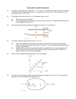


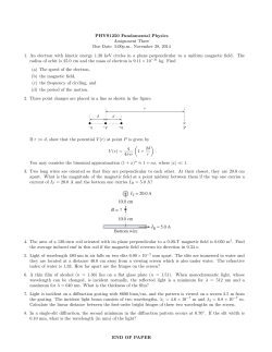

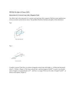


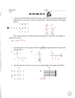
© Copyright 2026