
Forecasting When it Matters: Evidence from Semi
Forecasting When it Matters: Evidence from Semi-Arid India Xavier Gin´e∗ World Bank Robert M. Townsend MIT James Vickery FRB of NY This draft: April 2015 Abstract Decision-making under uncertainty depends not only on preferences but also on subjective probabilities. We elicit from a sample of farmers their beliefs about the timing of the monsoon, which signals the optimal time to plant. We assess the accuracy of beliefs by comparing them to historical data and find substantial heterogeneity in beliefs and accuracy. More importantly, elicited beliefs can explain differences in observed behavior. We then investigate the sources of inaccuracy and find that they fit well the predictions of a simple model of costly acquisition of information: poorer farmers whose incomes are more dependent on the monsoon are more accurate. Finally, we show that accuracy leads to average income gains of 8 to 9 percent of rainfed agricultural production. Keywords: Information Acquisition, Expectations, Forecasting, Climate. JEL Codes: D81, D84, O13, Q54. ∗ Email addresses: [email protected], [email protected], and [email protected]. Financial support from CRMG, GARP and World Bank is gratefully acknowledged. We want to thank Kumar Acharya, the survey team at ICRISAT and specially Dr. K.P.C Rao for many discussions about agricultural practices in semi-arid India and for their efforts in collecting the survey data. Dr. Piara Singh from ICRISAT provided valuable help in computing rainfall absorption of different soil types. We also thank Jean Marie Baland, Abhijit Banerjee, Shawn Cole, Adelaine Delavande, Quy-Toan Do, Pascaline Dupas, Michael Kremer, Lance Lochner, Hanan Jacoby, David McKenzie, Mark Rosenzweig, Chris Udry and participants in several conferences and seminars for valuable comments. Paola de Baldomero Zazo, Francesca de Nicola, Joan Pina Mart´ı and Laxman Timilsina provided outstanding research assistance. The views expressed in this paper are the authors’ and should not be attributed to the World Bank, Federal Reserve Bank of New York or the Federal Reserve System. 1 Uttara chusi, yattara gampa. Wait for the Uttara rains; if they don’t come, leave the place. Telugu Proverb 1 Introduction Decision-making under uncertainty depends on preferences and the subjective probabilities that agents attach to the different states of nature. The literature has typically assumed that agents know the probability distribution and so differences in behavior are driven by differences in preferences. If one however allows for differences in both probability distributions and preferences, then a fundamental identification problem arises, since behavior can be explained by differences in preferences, beliefs or both (Manski, 2004). In this paper we elicit the subjective distribution of the monsoon onset, an event of critical importance to lives of individuals engaged in rainfed agriculture in semi-arid India. In these areas, weather risk is a major source of income fluctuations. Rosenzweig and Binswanger (1993), for example, find that the delay of the monsoon can have considerable negative effects on agricultural yield and profits. To cope with risk, households rely on ex-ante and ex-post strategies that typically trade expected profits for lower risk (Walker and Ryan, 1990; Morduch, 1995). One such strategy, particularly relevant to our purposes, is the choice of an optimal time to plant that coincides with the onset of the monsoon (Fein and Stephens, 1987; Rao et al., 2000 and Gadgil et al., 2002). Because the onset varies from year to year, deciding when to plant involves significant judgment. If farmers plant after the first rains, but subsequent rains are scattered and fall several days apart, the seeds may not germinate. Farmers are then forced to either replant or to abandon the crop altogether, both resulting in significant losses. On the other hand, being too conservative by postponing planting until one is certain that the monsoon has arrived is also costly, because yield will typically be lower (Bliss and Stern, 1982; Fafchamps, 1993; Rao et al., 2000 and Singh et al., 1994). 2 In short, when the first rains of the season come, farmers must assess whether these are just early pre-monsoon rains, in which case they should postpone planting, or whether the rains signal the onset of the monsoon, in which case they should plant immediately. Our data provide direct evidence that misjudging the actual arrival of the monsoon is costly. In 2006, about a quarter of our sample had replanted in the past and a full 73 percent had abandoned the crop at least once in the prior 10 years due to poor rains. In addition, the extra expenses required to replant are large, equivalent to 20 percent of total average production expenses. Thus, it seems that farmers would benefit greatly from having accurate beliefs about the onset of the monsoon. Our survey covers 1,050 farming households living in 37 villages in southern India. Experimental methods are used to first elicit the respondent’s subjective definition of the onset of the monsoon, and then its subjective calendar distribution. To elicit the subjective definition, each farmer reports the minimum depth of soil moisture that he would require to start planting. This measure is then converted into a quantum of rainfall using the absorption capacity of the respondent’s specific soil type. The subjective calendar distribution is obtained by giving each respondent 10 stones and a sheet of paper with boxes corresponding to 13-14 day calendar periods. The respondent is then instructed to distribute the 10 stones across the different boxes according to the likelihood that the monsoon starts in the calendar period indicated by each box (see Delavande et al. 2011a for a review of these methods). This elicitation method delivers subjective expectations that are quite heterogeneous, even within villages. To understand the implications of this heterogeneity, we develop a simple model that combines heterogeneity in beliefs, irreversible investment and costly information acquisition (as in, for example, Reis, 2006). Consistent with the data, the model predicts that in villages where the monsoon onset is more volatile, farmers plant later. Intuitively, if initial rains are not very informative about the onset of the monsoon, the option value of waiting for more information before 3 planting is higher. Second, farmers who believe the monsoon will start later are also more likely to plant later and to replant less. All of these findings are also consistent with the model and provide strong evidence that individuals use their subjective expectations to make decisions, even after controlling for self-reported proxies of risk aversion, discount rates and the actual start of the monsoon.1 The model also predicts that the accuracy of farmers’ beliefs are dictated by a simple cost-benefit analysis of information acquisition. We find that accurate farmers are poorer, with more rainfall dependent income and more likely to be credit constrained. Put differently, accurate farmers are less able to cope with weather risk and have livelihoods that are more dependent on the monsoon. Thus, accuracy is rationally explained by how relevant the event is to the forecaster (Brunnermeier and Parker, 2005), rather than by heuristics or “rules of thumb” (Kahneman, Slovic and Tversky, 1982; Rabin, 1998 or DellaVigna, 2009 for a review). Finally, we show that inaccuracy about the onset of the monsoon is costly. In particular, an improvement in our measure of accuracy from the 25th to the 75th percentile of the distribution would increase gross agricultural income by 8 to 9 percent. Similarly, accurate farmers are less likely to replant, suggesting that they made fewer planting mistakes. Of course, farmers that make mistakes have less at stake since their incomes depend less on the monsoon. More generally, because differences in behavior can be explained by differences in expectations independently of differences in preferences, these results advocate for the collection and use of expectations data to predict behavior. Distinguishing whether behavior is driven by preferences or beliefs is important because they result in different policy prescriptions. If farmers have accurate beliefs, and 1 We are not the first to show the predictive power of elicited subjective expectations. In other contexts, Bernheim and Levin (1989), Lochner (2007), van der Klaauw and Wolpin (2008), Delavande (2008), Mahajan et al. (2011) and Gin´e and Jacoby, 2015 all show that elicited beliefs predict observed behavior. 4 planting choices are driven by differences in preferences, then policies that distort those choices could be welfare reducing. In contrast, if differences in planting choices are the result of inaccurate beliefs, then policies that lower the cost of acquiring information could enhance welfare. Our results suggests that in a context where information is costly, interventions that only disclose information about an event will be ineffective because individuals that care about the event will have already gathered the information while individuals that do not care about it will not pay any attention to the information. This provides an explanation for the mixed evidence found in the literature about the impacts of information campaigns.2 More broadly, this paper contributes to a growing literature that measures expectations and its impacts on various outcomes (see Manski, 2004 for an excellent review; Norris and Kramer, 1990 for an early review of elicitation methods applied to agricultural economics or more recently, Attanasio, 2009; Delavande et al. 2011a and Delavande, 2013 that also review the literature in developing countries and advocate the collection of expectations data).3 While this literature shows that beliefs are sometimes systematically biased (for example, DellaVigna and Malmendier 2006 show that people signing up for gym memberships are overconfident about future attendance; Allcott 2013 shows that consumers under2 See for example Allcott (2011) and Ferraro et al. (2011) on energy and water conservation and Dupas (2009) and Ashraf et al. (2013) on health-related products. 3 Bernheim and Levin (1989) study how beliefs of social security benefits affects consumption, savings, and retirement decisions. Similarly, Dominitz and Manski (2007) uses beliefs on portfolio returns, van der Klaauw and Wolpin (2008) uses beliefs in life expectancy and Dominitz (1998) uses beliefs in future income to study similar decisions. Delavande (2008) studies how takeup of preventive birth control measures depend on expectations of their efficacy and Mahajan et al. (2011) examine the adoption of antimalarial insecticide-treated bednets in India. Lochner (2007) shows how perceived arrest probabilities correlate with individual characteristics and with future criminal behavior. Dominitz and Manski (1996), Jensen (2010), and Delavande and Kohler (2012) study perceived returns to schooling and educational choices, while McKenzie et al. (2013) study perceived returns to migration. Luseno et al. (2003) and Lybbert et al. (2007), study the extent to which cattle herders in Kenya update their priors on rainfall expectations in response to new information. Carroll (2003) and Mankiw, Reis, and Wolfers (2003) study inflation expectations, showing that consumers disagree and that individuals beliefs tend to lag those of professional forecasters. 5 estimate vehicle gas mileage and Jensen (2010) and McKenzie et al. (2013) show that individuals underestimate the returns to schooling and migration), we are the first ones to combine historical and survey data to assess individual heterogeneity in accuracy and its impacts on welfare. The rest of the paper is organized as follows. The next section presents a simple model and a set of testable predictions, Section 3 describes the context and the data collected, Section 4 takes the model predictions to the data and finally Section 5 concludes. 2 Theory Consider a risk-neutral farmer at the beginning of the growing season that after receiving some rain, decides whether to plant a rainfed crop or to wait. The benefit of waiting is that the farmer can make a more informed decision, which is valuable because if the farmer plants and the rains are not followed by more rains, the seeds may not germinate. The cost of waiting, however, is that planting immediately after the initial rains will increase total agricultural output if the monsoon has indeed arrived. The farmer has a prior about the timing of the onset of the monsoon that may differ from the objective probability. The farmer is endowed with a unit of attention which can be devoted to updating the prior of monsoon onset or to another activity that does not depend on the monsoon. In what follows, we first lay out the assumptions and we then characterize the optimal planting strategy, the expected profits from growing the rainfed crop, and the optimal choice of attention. The Online Appendix contains a more thorough derivation of the expressions and the proofs of the propositions. Timing of events. The timing of events is shown in Figure 1. There are three periods: 0, 1 and 2. The monsoon can arrive at the end of period 1 or in period 2. If the monsoon arrives at the end of period 1, the state s is “Onset” (s = O), while if it arrives in period 2, the state s is “Delay” (s = D). In period 0 the farmer decides how much 6 attention to pay updating the prior that the state is s = O. At the beginning of period 1, the farmer observes an initial amount of rain r, which can take on three values rH , rM or rL , rH > rM > rL . This initial rain r is informative of the state s in that state is correlated with the rain (see below). The farmer then chooses to either plant the rainfed crop or to wait. We assume that planting in period 2 is also profitable, and so farmers that did not plant in period 1, will do so in period 2. At the end of period 2, the farmer receives harvest income which depends on the state and the timing of planting. Income. If the farmer decides to plant in period 1, he obtains gross income y if the monsoon arrives at the end of period 1 (s = O) and 0 if the monsoon is delayed and arrives in period 2 (s = D). Planting costs are c > 0. If the farmer waits until period 2 to plant, he obtains gross income y, irrespective of the state. We assume that y > y > c, reflecting the cost of waiting to plant in period 2 when the state is s = O and that planting in period 2 is also profitable. Correlation between signal r and state s. The probability of observing signal rj , j = H, M, L conditional on state s, s = O or D is given by the following table: Pr(rj |s) rH rM rL O 3+2δ 9 3+δ 9 1−δ 3 D 1−δ 3 1−δ 3 1+2δ 3 The parameter δ measures the degree to which signal rj is informative. Updating of Priors. Farmers can devote the unit of attention a to updating their prior that the monsoon arrives at the end of period 1 (state s = O). We assume that posterior beliefs can be written as: µ b = µ + (1 − a), where µ is the objective probability of state s = O and follows a uniform distribution ∼ U [−, ]. 7 Landholdings. Farmers are endowed with rainfed and irrigated land. We denote by γ the share of the farmer’s land with access to irrigation that can be used to grow irrigated crop with (constant) net income yI . 2.1 Optimal Planting Decision The decision to plant in period 1 depends on the posterior beliefs µ b of the state s = O and signal informativeness δ. In particular, the expected utility of planting in period 1 conditional on observing signal rj , j = H, M, L can be written as Ey(Plant|rj ) = Pr(s = O|rj )(y − c) + Pr(s = D|rj )(−c) = Pr(s = O|rj )y − c. Similarly, the expected utility of waiting in period 1, conditional on observing the same signal rj is Ey(Wait|rj ) = y − c. The perceived unconditional probability of receiving signal rH , for example, can be written as 1 + 2δ πc µ b+ H = 9 1−δ 3 (1 − µ b), and using Bayes Law, one can write posterior beliefs of the state s = O conditional on observing signal rH as Pr(s = O|rH ) = Pr(rH |s = O)b µ = πc H 1+ 1 3(1−δ) 1−b µ 3+2δ µ b , with analogous expressions for Pr(s = O|rM ) and Pr(s = O|rL ) contained in the Online Appendix. cj be the difference in expected utility between planting and waiting in period 1 Let ∆ when signal rj is received. The farmer will plant if the expected gains from planting are 8 cj > 0. The gains from planting ∆ d positive, ∆ H as a function of δ can be written as d ∆ H (δ) = y 3(1−δ) 1−b µ 3+2δ µ b 1+ − y. d c The Online Appendix contains similar expressions for ∆ M and ∆L . It is easy to show d d c that ∆ H (δ) and ∆M (δ) (∆L (δ)) are increasing (decreasing) in signal informativeness δ. Expected gains evaluated at the objective probability µ of the state s = O are denoted by ∆j , j = H, M, L. Similarly, the unconditional probability of receiving signal rj evaluated at accurate beliefs µ is denoted πj , for all j = H, M, L. To make things interesting, we assume that with accurate beliefs (b µ = µ),the expected cj (0) = ∆j (0) < 0 for j = H, M, L. In words, whenever rL gains from planting satisfy ∆ is observed and beliefs are accurate, it is always optimal to wait irrespective of the signal informativeness δ.4 cj (δ) for j = H, M, L assuming that ∆ cj (0) < 0 for Figure 2 plots the functions ∆ j = H, M, L. The optimal planting strategy for the farmer when the signal is rH (rM ) is to c plant, whenever δ ≥ δc H (δ ≥ δM ). If rL is received, the farmer should wait because in this cL (δ) < 0, for all values of signal informativeness δ. Thus, signal informativeness case, ∆ plays an important role in the optimal planting strategy, as stated in our first proposition. cj (0) < 0 for j = H, M, L, the amount of rain required to plant in Proposition 1 If ∆ period 1 is (weakly) decreasing in signal informativeness δ. The optimal planting strategy can also be written in terms of posterior beliefs µ b. Upon receiving signal rj , the farmer will plant if posterior beliefs satisfy µ b > µj , where cutoffs µj depend on signal informativeness δ. It is clear that farmers with higher posterior beliefs µ b are more likely to plant in period 1 as stated in the next proposition. Proposition 2 The probability of planting in period 1 is (weakly) increasing in posterior beliefs µ b of state s = O. 4 This assumption is satisfied as long as µ < c+y y . 9 2.2 Expected Profits Expected profits EY from growing the rainfed crop when posterior beliefs are accurate (b µ = µ) can be written as EY = y−c for δ < δH πH Ey(Plant|rH ) + (1 − πH )(y − c) = y − c + πH ∆H y−c+π ∆ +π ∆ H H M M for δH ≤ δ < δM (1) for δM ≤ δ because it is never optimal to plant when δ < δH , it is only optimal to plant if rH is observed when δH ≤ δ < δM , and it is optimal to plant when either rM or rH is observed when δ ≥ δM . In contrast, expected profits EY with inaccurate posterior beliefs (b µ 6= µ) can be written as EY = y − c + X πj Pr(b µ ≥ µj )∆j . (2) j=H,M,L The main difference between (1) and (2) is that Pr(b µ ≥ µj ), j = H, M, L appear in (2) but not in (1). With accurate beliefs, Pr(µ ≥ µj ) j = H, M is either 0 or 1 depending on actual informativeness δ, and Pr(µ ≥ µL ) = 0 always by assumption. The probabilities Pr(b µ ≥ µj ), j = H, M, L reflect the possibility of planting mistakes, as farmers that should have planted may decide to wait, and farmers that should have waited may decide to plant. Note that as shown in the Online Appendix, probabilities πj and gains to planting ∆j , j = H, M, L in both expressions (1) and (2) are identical because they are all evaluated using the objective probability µ of state s = 0. According to expression (1) when signal informativeness δ satisfies, for example, δ < δH , it is optimal to wait and expected profits are EY = y − c. In contrast, since posterior 10 beliefs depend on attention a, expected profits EY (a) when δ < δH , are: P y − c + j=H,M,L πj Pr(b µ > µj )∆j P y−c+ µ > µj )∆j j=H,M πj Pr(b EY (a) = µ > µH )∆H y − c + πH Pr(b y−c for a ∈ [0, a ¯0L ) for a ∈ [¯ a0L , a ¯0M ) for a ∈ [¯ a0M , a ¯0H ) for a ∈ [¯ a0H , 1] where attention cutoffs a ¯0L < a ¯0M < a ¯0H < 1 are derived in the Online Appendix. Since δ < δH , the gains from planting are always negative, ∆j < 0, j = H, L, M . As a result, lower investments in attention a to update the prior of state s = O lead to lower expected profits because more negative terms (∆j < 0) appear in the expression above.5 We state this result in the form of a proposition: Proposition 3 The more inaccurate posterior beliefs of state s = O are, the lower are expected profits from rainfed crops. Figure 3 plots expected profits EY as a function of attention a for different levels of signal informativeness δ. As stated in Proposition 3, expected profits are (weakly) increasing in attention a. The functions have kinks at the different attention cutoffs, and as attention a increases, the probability of mistakes decreases and expected profits become flatter. These flat segments are longer as signal informativeness δ increases creating a substitution between attention a and informativeness δ. In the extreme when the signal is conclusive δ = 1, posterior beliefs and hence attention a do not matter and expected profits are constant. Appendix Figure 1 plots expected profits EY as a function of signal informativeness δ for three levels of attention a: a = 1 corresponding to accurate posteriors (b µ = µ), a = 0.5 and a = 0 corresponding to inaccurate priors. Finally, Figure 4 plots expected profits EY (a, δ) both as a function of attention a and of signal informativeness δ. 5 The Appendix contains the expressions for EY (a) when δH < δ < δM and δM < δ. In all cases, expected profits increase as attention a increases. 11 To be clear, we consider a “mistake” the decision to plant (before the state is revealed) when a farmer with accurate beliefs would have waited, or viceversa, the decision to wait when the farmer with accurate beliefs would have planted. Other ex-post errors made by farmers with accurate beliefs such as planting when in fact the monsoon was delayed (s = D), or waiting when the monsoon actually arrived in period 1 (s = O) are not considered “mistakes” because they represent the best decision given available (and accurate) information. 2.3 Choice of Attention The farmer allocates the unit of attention to solve the following problem: (1 − γ)EY (a; δ) + γyI (1 − a) maxa s.t. 0 ≤ a ≤ 1 Clearly, the larger the returns to the irrigated crop yI or the larger the fraction of land with irrigation, the less attention will be devoted to updating the priors. More in general, farmers with access to irrigated crops whose net income do not depend on accurately predicting the timing of the monsoon, will tend to have less accurate beliefs, as stated in the next proposition. Proposition 4 The less relevant the monsoon is to overall net income, the less accurate will posterior beliefs be. 3 Data and Context This paper uses household survey data and historical rainfall data to test the predictions of the model. Survey data were collected using a specialized survey that was also designed to evaluate a rainfall insurance pilot program described in Gin´e, Townsend and Vickery 12 (2008) and Cole et al. (2013). The survey took place after the 2004 harvest, and covered 1,051 households in 37 villages from two drought prone and relatively poor districts in the states of Andhra Pradesh and Telangana, India. We resurveyed the same households in 2006, 2008, 2009 and 2010, so a few variables are constructed using these later rounds.6 Survey villages are assigned to the closest rainfall gauge, typically located less than 5 miles away. There are five rainfall gauges in Mahbubnagar district and five in Anantapur district. Table 1 presents the number of villages and households assigned to each rainfall gauge, the average distance from each gauge to the villages assigned to it and the number of years with available daily rainfall data. Table 2 presents summary statistics of the respondents’ household characteristics, their land characteristics and of other variables used in the analysis.7 The average household head is 47 years old and has been farming for 25 years. Thirty percent of households have a member older than 60 whose experience in farming could be used by the head in updating his priors about the onset.8 The head of household has an average of 3.3 years of schooling and a literacy rate (measured by the self-reported ability to read and write) of only 37 percent. Respondents cultivate on average 6.28 acres valued at Rs. 246,000 (USD 5,234) and the value of the households’ primary dwelling averages Rs 69,000 (USD 1,468), thus confirming that the sample consists mostly of smallholder farmers. Table 2 also includes the percentage of land with different textures, the prevalence of intercropping and the slope and depth of the top soil of their plots.9 The bottom of Table 6 The sampling framework used a stratification based on whether the household attended a marketing meeting and whether the household purchased a deficit rainfall insurance policy in 2004. Within each strata, households were randomly selected. 7 Appendix Table A1 contains a detailed description of how variables are constructed. All statistics in Table 2 are weighted by the sampling weights. See Gin´e, Townsend and Vickery, 2008 for further details. 8 Rosenzweig and Wolpin (1985) develop a theory that explains the predominance of intergenerational family extension, kin labor and the scarcity of land sales from the fact that elders have experiential knowledge about farming practices specific to the plots of land owned by the household. 9 Intercropping is frequently used in the semi-arid tropics and consists of growing two (or more crops) in the same plot planted at the same time, alternating one or more rows of the first crop with one or more rows of the second, possibly in different proportions. One crop will typically be shallow rooted, while the other will be long-rooted, ensuring that crops do not compete for soil nutrients at the same soil depth. 13 2 reports basic cropping patterns followed by our sample of farmers. Interestingly, most farmers plant all the rain sensitive crops at once, instead of planting different plots at different times as a way to diversify risk. They do so because of the relatively high fixed costs of land preparation and the prevalence of intercropping that requires that crops be sown at the same time. The main cropping season runs from June to November coinciding with the monsoon. Farmers grow a variety of cash and subsistence crops that vary in their yield’s sensitivity to drought. The main cash crops grown in the area are castor (mostly in Mahbubnagar, covering 34 percent of the cultivated area), groundnut (covering half of the cultivated area in Anantapur) and paddy (grown in both disticts and covering 9 percent of cultivated area in the sample). The main subsistence crops are grams and sorghum (covering less than 10 percent each). All crops with the exception of paddy are rainfed (less than 5 percent of plots are irrigated). Paddy is almost exclusively irrigated (84 percent of all plots use groundwater irrigation only available to wealthier farmers). Table 2 reports that farmers in Anantapur tend to plant later, around July 6 while farmers in Mahbubnagar plant around June 15th. Thus, farmers in Anantapur plant much later than the normal onset date of June 3rd according to the Indian Meteorological Department (IMD), drawn in grey in Figure 6.10 According to our survey data, between 1996 and 2006, twenty-two percent of households replanted at least once, and almost three quarters had abandoned the crops at some point over the same period. The main reason for abandoning the crop is failure of the seed to germinate and either lack of capital to purchase additional seeds, or low expectations of subsequent rains to warrant replanting. In 2006, roughly 3 percent of the sample replanted some crop, spending an additional Rs 5,000 (USD 86) that accounted for 23 10 Murphy and Winkler (1984) describe the field of meteorology as one in which probability forecasts are very accurate, possibly due to the wealth of available data and the long tradition in forecasting. In contrast, this finding suggest that the IMD forecast of the onset of the monsoon is less accurate than the farmer’s expectations, perhaps because the focus of IMD’s forecast is unrelated to the optimal sowing time that farmers in a specific region should follow. 14 percent of total production costs. All in all, this evidence suggests that farmers could avoid costly mistakes by having accurate beliefs about the start of the monsoon.11 3.1 Onset of Monsoon We use two definitions of onset of the monsoon. The first definition is based on the respondent’s self-reported minimum quantum of rainfall required to start planting. The survey asked “What is the minimum amount of rainfall required to sow?” and also “What is the minimum depth of soil moisture required to sow?”. Only 10 percent of farmers provided an answer when asked in millimeters, but all farmers responded using the depth of soil moisture, so we used the soil’s absorption capacity to convert soil depth into millimeters of rainfall.12 We label this quantum of rainfall from each respondent, the “individual definition” of the onset. The second, or “district definition” is simply the average of the individual definitions just described for each district. The average onset of the monsoon in millimeters is 28.95 mm in Mahbubnagar and 33.05 mm in Anantapur.13 Figure 7 shows that there is volatility in the onset of the monsoon. It plots for a particular rainfall station in each district, the time that it took each year for daily rainfall to accumulate to the district definitions described above, measured in days since June 1st. For example, the left plot shows that according to the historical daily rainfall for the year 2000, it took 33 days for rainfall in the Hindupur gauge to accumulate to 33.05 mm, 11 Although what ultimately matters for a good harvest is total accumulated rainfall at key points of the cropping season, the onset of the monsoon (as defined in the next subsection) is correlated with total accumulated rainfall (p-value is 0.003). Thus, the later the onset, the lower will be accumulated rainfall during the cropping season (see also Rosenzweig and Binswanger, 1993 and Rosenzweig and Udry, 2014). 12 The calculations for rainfall penetration for various soil textures use the generic values of field capacities under the following assumptions: (i) The top soil (1-1.5 foot) is completely dry, (ii) no runoff occurs (iii) moisture is primarily determined by the texture and structure of the soil and (iv) evaporation from soil surface is ignored. 13 Since a given farmer may have plots of differing soil texture, the quantum of rainfall is computed as a weighted average of a millimeter amount for each soil texture, weighted by plot size. Eighty percent of cultivable land in Anantapur is red soil, with texture either loamy sand or loam, and the rest is black soil, with texture either silty clay or clay loam. Mahbubnagar has more of a balance, with 66 percent of the soil being red. See “Land Characteristics” in Table 2. 15 the average of the individual definitions in Anantapur district. In the same year (right graph), it only took 3 days for rainfall measured in Mahbubnagar to accumulate to its district definition. To be sure, by the time farmers decide when to plant, they may have received numerous signals about the likelihood that the monsoon will arrive in the coming days. If upon receiving such a signal, farmers knew with certainty the onset and therefore the optimal time to plant, then beliefs about the onset would be inconsequential to the planting decision, since they would simply wait for the conclusive signals. But a long and rich folk tradition of trying to predict the arrival of the monsoon rains indicate that these signals are noisy at best and that the prior distribution still matters as it affects the farmers’ conditional expectation as assumed in the model of Section 2.14,15 Indeed, Figure 8 shows that the onset of the monsoon conditional on the IMD forecast still displays substantial volatility.16 For a given year, it plots the difference in days between the actual onset of the monsoon plotted in Figure 6 and the forecast from the IMD. Figures 7 and 8 show that there is no trend in the start of the monsoon over time, consistent with Goswami et al. (2006) that finds that while there is no trend in the average accumulated rainfall over the season, the frequency of extreme events such as heavy rains and prolonged droughts increased over the period 1951–2000. Thus, global warming may have increased the variance of rainfall during the monsoon, but not necessarily its average 14 This accumulation of indigenous knowledge over thousands of years is reflected in the literature, folk songs, and proverbs or sayings. For example, farmers use the color of the sky, the shape and color of the clouds, the direction of the winds, the appearance of certain insects or migratory birds, and so on, to update the probability that the monsoon has arrived (Fein and Stephens, 1987). 15 In terms of the model in Section 2, the prior distribution is µ b and the conditional expectation is Pr(s = 0|rj ). 16 The IMD issues a single forecast of the onset of the monsoon over Kerala, around May 15th. We extrapolate this forecast to other regions adding the normal onset dates plotted in Figure 6 to the forecast over Kerala. Rosenzweig and Udry (2014) use the long-range rainfall forecast of the monsoon and show that in places where the forecast is more accurate agricultural investment decisions react more to the forecast. 16 nor its onset.17,18 The lack of a time trend in the timing of the monsoon is relevant because if such a trend existed, recent observations should carry more weight when constructing the historical distribution. In addition, both the onset of the monsoon in Figure 7 and the conditional onset of Figure 8 are more volatile in Anantapur than in Mahbubnagar (p-val of equal means is 0.000). In terms of the model of Section 2, it appears that signal informativeness in Anantapur is lower than in Mahbubnagar. In the Section 4 we will assess how farmers in Anantapur respond to this more erratic environment. 3.2 Consistency of Subjective Distributions The subjective distribution of the monsoon arrival is obtained experimentally by giving the respondent 10 stones and a sheet of paper with boxes corresponding to the different 13-14 day periods called “kartis”.19 The respondent is instructed to place all the stones in the different boxes according to his estimate of the likelihood that the monsoon would start in each period. The question does not specify any year in particular and should be interpreted as the respondent’s prior distribution of the onset of the monsoon. The simple model of Section 2 considers only 2 possible dates of monsoon arrival and thus the prior distribution we elicit boils down to a single number µ b. In practice, the monsoon can arrive anytime from early June to mid July and thus a multi-date support is required. More importantly, with the full distribution over a multi-period support we can use moments higher than the mean to assess behavior. 17 See also Gadgil and Gadgil (2006) and Mall et al. (2006) for further evidence on all-India climatic trends and a review of their effect on agriculture. 18 When we regress the onset date (in days since June 1st) against a linear and quadratic trend using year and rainfall station observations in each district (a total 170 observation in Anantapur and 158 in Mahbubnagar), neither the linear nor the quadratic coefficients are significantly different from zero (results not reported). 19 Kartis or naksatra in Sanskrit are based on the traditional solar calendar (Fein and Stephens, 1987; Gadgil et al., 2002) and were used by farmers to determine the timing of agricultural activities. 17 This method of elicitation has been successfully used elsewhere (Gin´e and Jacoby, 2014 for a recent example and Delavande et al. 2011a for a review). The fact that every respondent provided a subjective distribution and no respondent allocated less than the total 10 stones given also gives us confidence that the elicitation was successful. In addition, no respondent allocated a stone in the first or last period of the predefined support, indicating that it did not constrain the respondents’ answers.20 Table 3 provides further evidence of the consistency of subjective distributions as compared to the historical ones, computed both under the “individual” and “district” definitions. The highest and lowest bin in the support of both the subjective and historical distributions are remarkably similar, except perhaps in Anantapur, where respondents seem to underestimate the range. In addition, most respondents put stones in 3 or 4 different bins, and no respondent puts all 10 stones in a single bin, suggesting perceived uncertainty about the onset. In their theory of optimal expectations, Brunnermeier and Parker (2005) suggest that insofar as individuals derive utility from an early monsoon, they would tend to predict the onset to arrive earlier. We do not find evidence that the mean of the subjective distribution is lower than that of the historical distribution using either definition. If anything, the subjective mean is higher. There is however some evidence of over-confidence since the standard deviation of the subjective distribution is lower than that of the historical distribution under either definition (p-value is 0.000 in both cases). 20 One concern is that respondents are constrained by the limited number of stones given, especially in Anantapur where there is more uncertainty about the start of the monsoon. If that were true, then the predictions in Anantapur would be less accurate. However, as we show below, respondents in Anantapur report distributions that match more closely the historical distribution. Delavande et al. (2011b) compare the accuracy of eliciting distributions with 10 or 20 stones and concludes that the number of stones does improve accuracy but only when the number of support points is large. 18 3.3 Accuracy We measure the accuracy of beliefs by computing a simple chi-square statistic for binned data. Let Hk be the number of years of available data when the monsoon arrived in kartis k as recorded in the rainfall station assigned to the respondent, and Sk the number of stones (from the available ten stones), that the respondent placed in the same kartis k. Because the number of years is different from the number of stones, the chi-square statistic is χ2 = X( k p p S/HHk − H/SSk )2 , Hk + Sk (3) where S= X Sk and k H= X Hk , k and k indexes the kartis. This statistic follows a chi-square distribution with degrees of freedom given by the number of bins (i.e. kartis in the sheet of paper given to the respondent) minus 1.21 Table 3 reports the percentage (appropriately weighted) of individuals in each district whose subjective distribution is statistically different from the historical ones at different significance levels. Accuracy is lower with the individual definition as compared to its average across respondents in the district, perhaps because inaccurate forecasters miss both the timing of the onset of monsoon as well as its definition. With the district average, mistakes across respondents are compensated in such a way that the respondents’ subjective distribution of the timing of the onset is closer to the historical distribution, thus appearing to be more accurate. In total, 40 percent of households in Mahbubnagar but only 20 percent in Anantapur report a subjective distribution that is significantly different at the 10% level from the historical one computed using the individual subjective definition. These numbers are 21 See Press (1992) for further details and references. 19 23% and 14% when the district average of individual definitions is used. It appears that respondents are more accurate in Anantapur where the onset is more volatile, and thus where it matters more, but we will explore these differences more formally in the next section. 4 Empirical Analysis and Results In this section we formally test the propositions derived from the model of Section 2. 4.1 Uncertainty and irreversible investments In Figure 8 described in Section 3, we showed that the conditional onset of the monsoon is more erratic in Anantapur district than in Mahabubnagar. Proposition 1 of the model states that in places with more uncertainty, or equivalently, where signals are less informative, farmers wait longer before incurring irreversible investments. We consider two such investments: the amount of rainfall required to plant and the purchase of inputs before the monsoon arrives. Both decisions have a certain degree of irreversibility. As already discussed, the downside of planting too early is that the farmer may have to either replant or abandon the crop if the seeds do not germinate for lack of subsequent rains. Likewise, preparing the land for a certain crop and purchasing the seeds before the monsoon arrives may be costly if given the patterns of the rains, it is best for the farmer to plant some other variety or crop that requires another type of land preparation. To test Proposition 1, we run the following regression: 0 Yiv = αViv + Xiv β + δv + iv , where Yiv is the investment decision of farmer i in village v, Viv is the standard deviation of the conditional onset of the monsoon plotted in Figure 8, that is, the difference in days 20 from the IMD forecast until the onset of monsoon, Xiv are household level characteristics and δv are village dummies. The key coefficient of interest is α. When the dependent variable is the minimum amount of rainfall required to plant we expect α to be positive as households living in more volatile areas will require more rain to start planting. Similarly, when the dependent variable is the percentage of expenditure before the monsoon we expect α to be negative as households facing more volatility will wait for the actual onset to purchase the agricultural inputs. Table 4 reports the results. All regressions include land, household controls and the stratification variables. The dependent variable in columns (1)-(3) is the amount of rain in millimeters that respondents require to start planting and in columns (4)-(6) it is the percentage of all agricultural expenditures made before the onset of the monsoon. Columns (1)-(2) and (4)-(5) use the individual definition of onset while columns (3) and (6) use the district definition to compute the standard deviation of the conditional onset of the monsoon Viv . Consistent with Proposition 1, the proxy for uncertainty is positive and significant in columns (1)-(3) and negative in columns (4)-(6) (albeit only significant in column 4). The coefficient on risk aversion is positive, as expected, but not precisely estimated. According to column 2, an increase of one standard deviation in volatility Viv is equivalent to waiting 3.6 additional days to plant and to reducing input expenditures before the monsoon by 1.7 percent. 4.2 Do beliefs affect behavior? Proposition 2 states that the probability of planting early is increasing in the belief of an early onset. We test this hypothesis more generally by assessing whether the behavior of respondents is influenced by their beliefs. We use the mean of the subjective distribution as a proxy for the household’s beliefs about the timing of the monsoon onset. To test the 21 correlation between beliefs and decisions, we estimate the following set of regressions: 0 γ + δiv + iv , Yiv = αµSiv + βriv + δkiv + Xiv where Yiv are production decisions taken by individual i in village v, µSiv is the mean in kartis of the subjective distribution (the expected onset of the monsoon in kartis) and α is the coefficient of interest. The variable riv is the individual definition of the monsoon in millimeters (minimum amount of rainfall required to start planting) and is included to isolate differences in the expected timing of the monsoon from differences in the individual definition. The variable kiv is the actual onset of the monsoon computed using the individual definition.22 We include it to isolate the influence of the subjective distribution on behavior, because it captures all the information available to the farmer when planting decisions are made. Put differently, we assess the relative importance of the unconditional vis a` vis the conditional expectation. The vector Xiv includes household characteristics that may influence decision-making, in particular risk aversion and the discount rate. We would expect that risk averse individuals would be more inclined to purchase insurance, to plant later, to replant less and to make fewer purchases before the monsoon. Similarly, individuals that discount more heavily the future would also tend to plant later and make fewer purchases before the monsoon as these costly activities are pushed into the future. Finally, we include village dummies δiv to focus on within village variation in behavior. We consider five production decisions Yiv , some of which are measured in multiple rounds. First, whether the household attended an insurance marketing meeting in 2004 in column (1) of Table 5. Second, whether the household bought rainfall insurance in 2004 (conditional on having attended the marketing meeting) in column (2).23 The insurance 22 We only have one rainfall gauge with available data in 2004 in Anantapur and three in Mahbubnagar. Based again on minimum distance, we reassigned villages to the next closest gauge with available data. 23 Insurance policies were not advertised outside the marketing meeting, and therefore most farmers that did not attend the meeting would not have heard about the insurance product. 22 policy paid out if accumulated rainfall during the coverage period was below a certain trigger. Because the end date of the policy coverage period was predetermined, households that believe that the monsoon would start late would also believe that the probability of a payout was higher as there would be fewer rainy days during the coverage period. The prediction therefore is that households that expect a later onset, would be more likely to purchase insurance. Third, we consider the average kartis in which the household planted in 2004, 2006, 2008 and 2009, averaging across crops and plots cultivated. Proposition 2 predicts that households that expect a late onset of the monsoon will also plant later. Fourth, we consider in column (4) whether the household has replanted in 2006 or in any of the previous 10 years. The prediction here is that households that believe that the monsoon will start later should have a lower probability of replanting, because by the time they plant the rains have likely arrived. Finally we look in column (5) at the percentage of expenditures before the actual onset of the monsoon in 2006 and 2009. Again, households that believe that the monsoon will start later will make fewer purchases before the monsoon actually sets in, although they would have liked to purchase inputs in advance to be prepared for the onset of the monsoon. The results are reported in Table 5 and provide strong evidence that the prior distribution of the monsoon onset is a powerful predictor of behavior in the expected direction. In column (2) the coefficient indicates that individuals that believe that the monsoon will arrive late are more likely to purchase the insurance product.24 The number of observations in columns (1) and (2) is lower because insurance marketing meetings took place in a subset of villages and column (2) only includes individuals that attended the meeting. In column (3) the coefficient implies that an increase of one kartis in the mean of the subjective distribution of the monsoon onset would delay planting by roughly 0.4 kartis or approximately one week. In column (4) it suggests that an increase of one kartis in the 24 Notice that risk aversion is significant but negative, implying that more risk-averse households are less likely to purchase insurance. This contradictory result is discussed in detail in Gin´e, Townsend and Vickery (2008). 23 mean of the beliefs distribution reduces the probability that the household has replanted in 2006 or in any of the previous 10 years by 5.4 percent. In column (5) the coefficient has the expected sign but is not statistically significant. As reported in Table 4 columns (4) and (5) the variation in the percentage of expenditures variable comes from differences across villages rather than differences within villages and therefore the inclusion of village dummies wipes out most of the variation.25 In contrast to the explanatory power of the prior distribution, the proxies of risk aversion or discount rates do not explain behavior except for column (2). All in all, these results are remarkable because they not only validate the elicitation method, but also indicate that heterogeneity in beliefs, more so than heterogeneity in preferences, explain actual behavior. 4.3 Who has accurate beliefs? We now turn to test Proposition 3 and compare the subjective prior distribution of the onset of the monsoon with the historical one, computed using both definitions for the onset of the monsoon. According to Proposition 3, accuracy depends on how relevant the production of rain-sensitive crops is to overall income. The specification we run is the following: 0 log(χ2iv ) = Zv0 α + Xiv β + iv where χ2iv is the chi-square statistic computed according to the formula in (3) for individual i in village v. A higher value of χ2iv indicates less accurate beliefs relative to the historical distribution. The vector Zv contains village-level variables such as a district dummy, the proxy for uncertainty described in the previous subsection and the distance from village v to the rainfall gauge. The vector Xiv includes a set of household level characteristics that may affect accuracy. These variables are described in Section 3, and include basic 25 Similarly to Table 4 column (4) the coefficient of interest is negative and statistically significant when village dummies are not included. 24 demographics, such as caste, literacy and education, wealth, the ability to cope with income shocks and exposure to weather shocks. A positive and significant coefficient on the variable Xivs would indicate that Xivs reduces accuracy, since higher χ2ivs values are associated with larger differences between the prior subjective and historical distribution. Table 8 reports the results. In columns (1)-(3), the historical distribution is computed using the district average of the individual definitions of the onset of monsoon while in columns (4)-(6), the individual definition is used. Columns (1)-(2) and (5)-(6) include village covariates, while columns (3) and (7), our preferred specification, include village dummies. Columns (4) and (8) report the p-value of an F-test that variables are jointly insignificant for this specification that includes village dummies. The district dummy in columns (2) and (6) is significant, suggesting that after controlling for household characteristics and other village controls, beliefs for respondents in Anantapur are less accurate. Distance to the rainfall gauge is significant and positive in columns (1) and (5), indicating that the possible lower correlation between the timing of rainfall at the gauge and at the village (basis risk) is partly responsible for the observed inaccuracy in the data. Variables that proxy for parameters in the utility function do not seem to influence accuracy. The lowest p-value of an F-test that variables are jointly insignificant is 0.35. Other demographic variables such as literacy, age and caste improve accuracy but they are estimated very imprecisely. Thus, accuracy is not about cognition per se, since literacy (or education) do not seem to influence it significantly. An F-test that all demographic variables are jointly insignificant cannot be rejected at the 10 percent (lowest p-value is 0.19).26 More interestingly, the wealthier the household as measured by the log value of the primary dwelling or the log value of the landholdings, the worse the household is in 26 The only household characteristic that appears significant is the Herfindahl index of soil type. Because the minimum moisture required to plant (ie the individual definition of the onset) depends on the soil type, farmers with different soil types will have a harder time reporting the correct definition and so will tend to be inaccurate. 25 recalling the monsoon arrival. An F-test that both wealth variables are jointly insignificant is always rejected at the 10 percent. Other variables that proxy for the ability to cope with shocks in general, such as per capita income, participation in a chit fund or being credit constrained are mostly significant and of the expected sign. The F-test is rejected in column (7) but not in column (3). In addition, variables that are correlated with the exposure to weather shocks, such as the amount of land the household cultivates (positive correlation) and the percentage of land devoted to rainfed crops are also of the right sign and mostly significant. The F-test is always rejected at the 10 percent level. In sum, confirming the prediction of the model, households whose incomes depend more heavily on the monsoon and households that lack proper risk-coping mechanisms to smooth weather shocks predict better the onset of the monsoon. Thus, households for which the monsoon is important are willing to devote resources (perhaps attention?) to acquire more information and are thus on average more accurate. 4.4 Does Accuracy Matter? According to Proposition 4 of the model, inaccuracy increases the scope for mistakes in the timing of planting, thus farmers with less accurate beliefs should experience lower yields of rainfed crops and should be more likely to replant. To test Proposition 4 we first estimate the following yield and profit regression ycit = α0 log(χ2i ) + αN P log(χ2i ) × DN P + Dc + Dt + Di + (4) DN P × Dt + log(χ2i ) × Dt + Xic0 β + cit , where ycidt is the yield per acre of crop c grown by farmer i in year t or total profits of crop c grown by farmer i in year t, where profits are computed by subtracting labor costs from the value of production. The variables Dc is a crop c dummy, DN P is a dummy that takes value 1 if the crop is rainfed, that is, if the crop is not paddy (No Paddy dummy), 26 Dt is a year dummy, Di is an individual dummy, log(χ2i ) is the log of the accuracy proxy χ2 according to the formula in (3), and Xc is a set of plot characteristics aggregated by crop and individual, that includes soil characteristics and the use of intercropping, among others. We use crop yields for 2004 and 2006, the years for which we have data.27 Since we have multiple crop observations per households we include household fixed effects and we cluster standard errors at that level. Second, we estimate the same specification of Table 5 including log(χ2i ) as a regressor. Ri = αχ log(χ2i ) + αµ µSi + βri + δki + Xi0 γ + i , where Ri is whether the household has replanted in 2006 or any of the prior 10 years and consumption in 2004, 2006 and 2007. The variable of interest is αχ . Panel A of Table 7 reports the results from regression (5). In columns (1) and (2) we find that lower accuracy results in lower yields for rainfed crops relative to paddy yields. As discussed, paddy is an irrigated crop and thus its cultivation is less subject to the vagaries of the monsoon. Because the coefficient in the variable log(χ2i ) is hard to interpret, we compute the increase in agricultural production for an individual with average landholdings growing rainfed crops, if accuracy were increased from the 25th percentile of the distribution to the 75th percentile.28 We find an average gain between Rs 1,500 and Rs 1,800 depending on the definition is used. These income gains translate into 7.8 percent and 9.1 percent of the total value of agricultural production or 5.3 percent and 6.1 percent of total household income. It is perhaps remarkable that we find income gains with only two years of data as one would have required a longer time series. In the regression however we exploit geographical variation in the timing of the monsoon onset, accuracy and timing of planting from multiple plots per households. In columns (3) and (4) we note that the coefficient of interest is less precisely estimated. 27 In later data collection rounds yields at the plot level are not available. The gains in yields per acre are converted into Kg for each crop using the average land size devoted to them, then Kg are multiplied by the respective prices and they are finally aggregated. 28 27 Columns (1)-(3) of Panel B presents strong evidence that more accurate beliefs are correlated with a lower probability of having replanted in the past. If accuracy increases from the 25th percentile of the distribution to the 75th percentile, the probability of replanting falls by 5.3 percent or 5.8 percent depending on the definition of onset used. More accurate beliefs are also correlated with higher consumption levels but the coefficients are not statistically significant. 4.5 Discussion The results indicate that accuracy of beliefs vary across respondents, although the costs of acquiring information appears low given that the onset of the monsoon is publicly observable. Since accuracy is negatively correlated with wealth, perhaps farmers that appear less accurate simply had higher opportunity cost of their time and did not put as much effort answering the questionnaire, including the questions that elicited the subjective distribution. We test this hypothesis by correlating our proxy of inaccuracy log(χ2i ) with an index of correct answers to abstract questions about rainfall insurance. Because the correct answer to these questions required the attention of the respondent, if the hypothesis is correct one would observe a negative correlation between inaccuracy and knowledge of insurance. As it turns out, columns (1) and (2) of Table 8 report a weak negative correlation as expected but one that is far from statistical significance. We conclude that our proxy for accuracy is not driven by the opportunity cost of time of the respondent or his lack of effort answering the survey. We note that if insurance markets were perfect within a village and households diversified risk by varying the timing of planting then accuracy would not be predictable and the inclusion of village fixed effects in Table 5 would wipe out the correlation between beliefs and behavior. However, since accuracy is predictable, even with village fixed effects we are able to reject the null of complete within-village insurance markets. More importantly, inaccurate farmers are more likely to make planting mistakes as ev- 28 idenced by their higher probability of replant and their lower yields. An obvious question is why inaccurate farmers do not imitate more successful neighbors in their planting and investment decisions? This strategy presupposes that inaccurate farmers know who the best forecaster is. Table 8 columns (3) to (6) show that inaccurate farmers are typically considered worse farmers by their peers and more importantly, in columns (7) and (8) they are less likely to predict who the good rainfed crop producers are. In columns (3) and (4) the dependent variable is a dummy for whether the respondent considers himself a progressive farmer. Columns (5) and (6) the dependent variable is the number of times a respondent is cited as being a good farmer of rainfed crops. In columns (7) and (8) the dependent variable is the number of times a respondent is cited as being a good farmer, so long as average yields of rainfed crops in 2004 and 2006 were in the top 25th percentile. The variable of interest is again log(χ2i ) and the coefficient tends to be negative and significant, suggesting that inaccurate farmers (with high χ2 ) are less likely to be considered either progressive farmers or good rainfed farmers and are also less likely to identify farmers with rainfed yields in the top 25th percentile. While in the model of Section 2 the variance of beliefs µ b does not play a role because there are only two states (s = 0 and s = D), more uncertainty in the subjective distribution (higher variance) may be correlated with more cautious behavior. Appendix Table 3 runs the same specification as that of Table 5 but includes the standard deviation of the subjective distribution alongside the mean of the subjective distribution. We find that the purchase of insurance and whether the household replanted (but not the timing of planting) are correlated with the variance more than the mean of the subjective distribution. 5 Conclusions In this paper we combine unique subjective expectations data with historical rainfall data to compute individual measures of accuracy. We find that individuals with stronger 29 incentives to gather information about the monsoon have more accurate beliefs. Consistent with a simple model of costly information acquisition, accuracy seems to be less explained by cognitive biases (Kahneman, Slovic and Tversky, 1982; Rabin, 1998) than by how relevant the event is to the individual. In addition, we show that the elicitation method used delivers informative prior subjective expectations and that there is significant heterogeneity in beliefs across households. More importantly, real outcomes, such as the timing of planting decisions and agricultural profitability, are strongly influenced by households’ beliefs about the monsoon. This suggests that expectations are a powerful predictor of behavior, even more so than proxies for parameters in the utility function and thus, eliciting expectations data is important and should be incorporated in the analysis of decision-making problems. References [1] H. Allcott. Social norms and energy conservation. Journal of Public Economics, 95(9):1082–1095, 2011. [2] H. Allcott. The Welfare Effects of Misperceived Product: Data and Calibrations from the Automobile Market. American Economic Journal: Economic Policy, 5(3):30–36, 2013. [3] N. Ashraf, B. K. Jack, and E. Kamenika. Information and subsidies: complements or substitutes? Journal of Economic Behavior and Organization, 88:133–139, 2013. [4] O. Attanasio. Expectations and Perceptions in Developing Countries: Their Measurement and Their Use. American Economic Review, 99(2):87–92, 2009. [5] B. D. Bernheim and L. Levin. Soical Security and Personal Savings: An Analysis of Expectations. American Economic Review, 79(2):97–102, 1989. 30 [6] C. J. Bliss and N. H. Stern. Palanpur, the Economy of an Indian Village. Oxford University, Oxford, England, 1982. [7] M. K Brunnermeier and J. A. Parker. Optimal Expectations. American Economic Review, 95(4):1092–1118, 2005. [8] C. D. Carroll. Macroeconomic Expectations of Households and Professional Forecasters. Quarterly Journal of Economics, 118(1):269–98, 2003. [9] S. Cole, X. Gin´e, J. Tobacman, P. Topalova, R. Townsend, and J. Vickery. Barriers to Household Risk Management: Evidence from India. American Economic Journal: Applied Economics, 5(1):104–135, 2013. [10] A. Delavande. Pill, Patch, or Shot? Subjective Expectations and Birth Control Choice. International Economic Review, 49(3):999–1042, 2008. [11] A. Delavande. Probabilistic Expectations in Developing Countries. National Bureau of Economic Research, 6:1–20, Forthcoming. First published online as a Review in Advance on December 20, 2013. [12] A. Delavande, X. Gin´e, and D. McKenzie. Measuring Subjective Expectations in Developing Countries: A Critical Review and New Evidence. Journal of Development Economics, 94:151–163, 2011a. [13] A. Delavande, X. Gin´e, and D. McKenzie. Eliciting Probabilistic Expectations with Visual Aids in Developing Countries: How sensitive are answers to variations in elicitation design? Journal of Applied Econometrics, 26(3):479–497, 2011b. [14] A. Delavande and H. P. Kohler. The Impact of HIV Testing on Subjective Expectations and Risky Behavior in Malawi. Demography, 49(3):1011–36, 2012. [15] S. DellaVigna. Psychology and Economics: Evidence from the Field. Journal of Economic Literature, 47(2):315–372, 2009. 31 [16] J. Dominitz. Earnings Expectations, Revisions, and Realizations. The Review of Economics and Statistics, 80(3):374–88, 1998. [17] J. Dominitz and C. F. Manski. Eliciting Student Expectations of the Returns to Schooling. Journal of Human Resources, 31(1):1–26, 1996. [18] P Dupas. What matters (and what does not) in households’ decision to invest in malaria prevention? . American Economic Review, 99(2):224–230, 2009. [19] M. Fafchamps. Sequential Labor Decisions Under Uncertainty: an Estimable Household Model of West African Farmers. Econometrica, 61(5):1173–1197, 1993. [20] J. Fein and P. Stephens. Monsoons. John Wiley and Sons, New York, NY, 1987. [21] P. J. Ferraro, J. J. Miranda, and M. K. Price. The persistence of treatment effects with norm-based policy instruments: evidence from a randomized environmental policy experiment. American Economic Review, 101(3):318–322, 2011. [22] S. Gadgil and S. Gadgil. The Indian Monsoon, GDP and Agriculture. Economic and Political Weekly, November 25:4887–4895, 2006. [23] S. Gadgil, P.R. Seshagiri Rao, and K. Narahari Rao. Use of Climate Information for farm-level decision making: rainfed groundnut in southern India. Agricultural Systems, 74:431–457, 2002. [24] X. Gin´e and H. Jacoby. Markets, Contracts, and Uncertainty: A Structural Model of a Groundwater Economy. World Bank, 2015. [25] X. Gin´e, R. Townsend, and J. Vickery. Patterns of Rainfall Insurance Participation in Rural India. The World Bank Economic Review, 22(3):539–566, 2008. [26] B.N. Goswami, V. Venugopal, D. Sengupta, M.S. Madhusoodanan, and Prince K. Xavier. Increasing Trend of Extreme Rain Events Over India in a Warming Environment. Science, 314(5804):1442–1445, 2006. 32 [27] R. Jensen. The (Perceived) Returns to Education and the Demand for Schooling. Quarterly Journal of Economics, 125(2):515–48, 2010. [28] D. Kahneman, P. Slovic, and A. Tversky. Judgment under Uncertainty: Heuristics and Biases. Cambridge University Press, Cambridge, UK, 1982. [29] L. Lochner. Individual Perceptions of the Criminal Justice System. American Economic Review, 97(1):444–60, 2007. [30] W. Luseno, J. McPeak, C. Barrett, G. Gebru, and P. Little. The Value of Climate Forecast Information for Pastoralists: Evidence from Southern Ethiopia and Northern Kenya. World Development, 31(9):1477–1494, 2003. [31] T. Lybbert, C. Barrett, J. McPeak, and W. Luseno. Bayesian herders: asymmetric updating of rainfall beliefs in response to external forecasts. World Development, 35(3):480–497, 2007. [32] A. Mahajan and A. Tarozzi. Time Inconsistency, Expectations, and Technology Adoption: The Case of Insecticide Treated Nets. U.C. Berkeley, 2011. [33] R. Mall, R. Singh, A. Gupta, G. Srinivasan, and L.S. Rathore. Impact of Climate Change on Indian Agriculture: A Review. Climatic Change, 78(2-4):445–478, 2006. [34] N. G. Mankiw, R. Reis, and J. Wolfers. Disagreement about Inflation Expectations. National Bureau of Economic Research, 18:209–70, Macroeconomics Annual 2003. edited by Mark Gertler and Kenneth Rogoff. [35] C. Manski. Measuring Expectations. Econometrica, 72(5):1329–76, 2004. [36] D. McKenzie, J. Gibson, and S. Stillman. A Land of Milk and Honey with Streets Paved with Gold: Do Emigrants Have Over-Optimistic Expectations about Incomes Abroad? Journal of Development Economics, 102:116–127, 2013. 33 [37] J. Morduch. Income Smoothing and Consumption Smoothing. Journal of Economic Perspectives, 9(3):103–114, Summer 1995. [38] A. Murphy and R. Winkler. Probability Forecasting in Meteorology. Journal of the American Statistical Association, 79(387):489–500, 1984. [39] P. Norris and R. Kramer. The Elicitation of Subjective Probabilities with Applications in Agricultural Economics. Review of Marketing and Agricultural Economics, 58(2-3):127–147, 1990. [40] W. H. Press. Numerical Recipes in C. Cambridge University Press, Cambridge, UK, 1992. [41] M. Rabin. Psychology and Economics. Journal of Economic Literature, 36:11–46, 1998. [42] K. N. Rao, S. Gadgil, P. R. Seshagiri Rao, and K. Savithri. Tailoring strategies to rainfall variability – The choice of thesowing window . Current Science, 78(10):1216– 1230, 2000. [43] R. Reis. Inattentive Producers. Review of Economic Studies, 73:793–821, 2006. [44] M. Rosenzweig and H.P Binswanger. Wealth, Weather Risk and the Composition and Profitability of Agricultural Investments. The Economic Journal, 103(1):56–78, 1993. [45] M. Rosenzweig and C. Udry. Forecasting Profitability. Yale U., 2014. [46] M. Rosenzweig and K. Wolpin. Specific Experience, Household Structure, and Intergenerational Transfers: Farm Family Land and Labor Arrangements in Developing Countries. Quarterly Journal of Economics, 100(Supplement):961–987, 1985. [47] P. Singh, K.J. Boote, A. Yogeswara Rao, M.R. Iruthayaraj, A.M. Sheik, S.S Hundal, R.S. Narang, and Phool Singh. . Field Crops Research, 39:147–162, 1994. 34 [48] W. van der Klaauw and K. Wolpin. Social Security and the Retirement and Savings Behavior of Low-Income Households. Journal of Econometrics, 145(1–2):21–42, 2008. [49] T. Walker and J. Ryan. Village and Household Economics in Indias Semi-Arid Tropics. John Hopkins University Press, Baltimore, Maryland, 1990. 35 Online Appendix: Details of the Model This Appendix derives expressions of the model in the text and provides the proofs to the propositions. Expected gains from planting The difference in expected utility between planting and waiting in period 1 when signal rj is received ∆j can be written as ∆j = Ey(Plant|rj ) − Ey(Wait|rj ) = = Pr(s = O|rj )(y − c) + Pr(s = D|rj )(−c) − (y − c) = Pr(s = O|rj )y − y. d The text reports the expression for ∆ H (δ). Using the expressions for Pr(s = O|rj ), j = M, L we have d ∆ M (δ) = y 1+ 3(1−δ) 1−b µ 3+δ µ b −y cL (δ) = and ∆ y 1+ (1+2δ) 1−b µ 1−δ µ b − y. Note that when the signal is uninformative (δ = 0), then d d c ∆ by − y, H (0) = ∆M (0) = ∆L (0) = µ (1) and when it is conclusive (δ = 1), then d d ∆ H (1) = ∆M (1) = y − y cL (1) = −y. and ∆ cj (δbj ) = 0 and can be written as The cutoff values δbj , j = H, L, M are defined by ∆ δc H = 3(y − µ by) 2b µ(y − y) + 3(1 − µ b)y and δbL = and δc M = 3(y − µ by) µ b(y − y) + 3(1 − µ b)y µb µ−y . µ b(y − y) + 2(1 − µ b)y It is easy to show that with accurate priors µ b = µ, then δbj = δj , for j = H, M, L and δL < 0 < δH < δM < 1 because by assumption y > y and µy < y. We now prove Proposition 1. First note that it only holds if posterior beliefs satisfy Assumption 1 below. Assumption 1 Posterior beliefs µ b satisfy µ b< 1 c+y . y Intuitively, since µ < c+y , y Assumption 1 states that posterior beliefs are sufficiently cj (0) < 0 for accurate. According to expression (1) above, Assumption 1 implies that ∆ j = H, M, L. Proposition 1 If Assumption 1 holds, the amount of rain required to plant in period 1 is (weakly) decreasing in signal informativeness δ. c Proof. Given Assumption 1, δbL < 0 < δc H < δM < 1. Consider first the case when signal informativeness δ is high at δH < δM < δ. Since in this case both ∆H (δ) > 0 and ∆M (δ) > 0, the farmer will plant if either rM or rH is received. For lower signal informativeness δ in the range δH < δ < δM , the farmer will only plant if signal rH is received and will wait if signal rM is received. Finally, if signal informativeness is even lower at δ < δH < δM , the farmer will always wait, even after receiving rH . If Assumption 1 does not hold, then c b 1 > δbL > 0 > δc M > δH . In this case if signal informativeness δ < δL then it is optimal to plant irrespective of the signal. For higher signal informativeness δ ≥ δbL the farmer will plant when signals rH and rM are received but will wait when signal rL is received. Thus, the amount of rain required to plant is increasing (not decreasing) with signal informativeness δ. We can express the optimal planting strategy in terms of posterior beliefs µ b as follows. Upon receiving signal rj , j = H, L, M , the farmer will plant if posterior beliefs satisfy µ b ≥ µj cj (µj ) = 0 and and will wait otherwise. The cutoff values µj , j = H, L, M are defined by ∆ can be written as µH = 3y(1 − δ) , 3y + δ(2y − 5y) µM = 3y(1 − δ) 3y + δ(y − 4y) and µL = y(1 + 2δ) . (1 − δ)y + 3δy It is easy to show that 0 ≤ µH ≤ µM ≤ µL ≤ 1 and that µL ∈ [ µL > µ because by assumption µ < c+y , 1] y always satisfies c+y . y Proposition 2 The probability of planting in period 1 is (weakly) increasing in posterior probability µ b of state s = O. Proof. Since the probability of planting in period 1 can be expressed as Pr(b µ > µj ), a farmer with higher posterior beliefs µ b is more likely to plant in period 1, for all levels of signal informativeness δ, because Pr(b µ > µj ) is higher. 2 Expected profits Expected profits can be written as EY = πH Pr(b µ ≥ µH )Ey(Plant|rH ) + (1 − Pr(b µ ≥ µH )) y − c + πM Pr(b µ ≥ µM )Ey(Plant|rM ) + (1 − Pr(b µ ≥ µM )) y − c + πL Pr(b µ ≥ µL )Ey(Plant|rL ) + (1 − Pr(b µ ≥ µL )) y − c which simplifies to EY = y − c + X πj Pr(b µ ≥ µj )∆j . j=H,M,L As mentioned in the text, the terms πj and ∆j , for j = H, M, L are evaluated at the objective probability µ instead of posterior beliefs µ b. We can use the framework of Brunnermeier and Parker (2005) (BP henceforth) to show that the expression for expected profits in () is correct. According to the BP framework, 1 hdi 1 E EY + EY = 2 " 2 # # " X X 1 1 cj + πbj Pr(b µ ≥ µj )∆ πj Pr(b µ ≥ µj )∆j = E y − c + y−c + = 2 2 j=H,M,L j=H,M,L h i cj πj ∆j + E πbj ∆ X . = y−c + Pr(b µ ≥ µj ) 2 j=H,M,L W = Now, Pr(rj |s = O)b µy − y πbj = πbj µ − Pr(rj |s = D)y(1 − µ b). = Pr(rj |s = O)(y − y)b h i cj = πj ∆j and W = EY , which is the desired result. Since E [b µ] = µ, then E πbj ∆ cj = πbj ∆ The probability of planting in () above can be written as, µj − µ Pr(b µ ≥ µj ) = Pr (µ + (1 − a) ≥ µj ) = Pr ≥ 1−a (2) where the bounds on can be computed assuming a = 0 and so µ + = 1 or = 1 − µ or µ− = 0, = −µ. Thus = min{1−µ, µ}. Without loss of generality, we assume henceforth that µ < 1 2 and so the bound is = µ. 3 Let cutoffs a ¯0j and a ¯1j be defined as follows. If Alternatively, if µj −µ 1−a ≤ − = −µ, then a ≥ µj µ µj −µ 1−a ≥ = µ, then a ≥ 2 − ¯1j = 2 so only ¯0j + a =a ¯1j . Note that a µj µ a ¯0j = a ¯0j . < 1 or a ¯1j < 1 can be true, but not both. Thus, because a ¯0j < 1 if and only if a ¯1j > 1 and viceversa, ¯1j depending on which one is less than 1. For the case of the relevant cutoff will be a ¯0j or a j = L, only a ¯0L is relevant because a ¯1L > 1 always. The probability in (2) simplifies to: ( 0 µj − µ Pr(b µ ≥ µj ) = Pr ≥ = 1 1−a − 2 if a ≥ a ¯0j µj −µ 2(1−a)µ otherwise, which is relevant when a farmer plants when he should have waited or ( 1 if a ≥ a ¯1j µj − µ = Pr(b µ ≥ µj ) = Pr ≥ µj −µ 1 1−a − 2(1−a)µ otherwise, 2 which is relevant when a farmer waits when he should have planted. In the text we report expected profits when signal informativeness δ satisfies δ < δH . In this case a mistake is made when the farmer plants because it is always optimal to wait. The relevant cutoffs are thus a ¯0j , j = H, M, L and expected profits are, for completeness: P y − c + j=H,M,L πj Pr(b µ > µj )∆j P y−c+ µ > µj )∆j j=H,M πj Pr(b EY (a) = y − c + πH Pr(b µ > µH )∆H y−c for a ∈ [0, a ¯0L ) for a ∈ [¯ a0L , a ¯0M ) ¯0H ) for a ∈ [¯ a0M , a for a ∈ [¯ a0H , 1] When signal informativeness δ satisfies δH ≤ δ < δM , mistakes are made when the farmer does not plant if rH is observed or if he plants when rM or rL are observed. The relevant cutoffs are thus a ¯1H and a ¯0j , j = M, L. Because a ¯1H could lie anywhere in a ¯0L < a ¯0M , we need to consider three different cases: If a ¯1H < a ¯0L < a ¯0M , P y − c + j=H,M,L πj Pr(b µ > µj )∆j P y−c+π ∆ µ > µj )∆j H H j=M,L πj Pr(b EY (a) = µ > µM )∆M y − c + πH ∆H + πM Pr(b y − c + πH ∆H 4 for a ∈ [0, a ¯1H ) for a ∈ [¯ a1H , a ¯0L ) for a ∈ [¯ a0L , a ¯0M ) for a ∈ [¯ a0M , 1]. If a ¯0L < a ¯1H < a ¯0M , P µ > µj )∆j y − c + j=H,M,L πj Pr(b P y−c+ µ > µj )∆j j=H,M πj Pr(b EY (a) = µ > µM )∆M y − c + πH ∆H + πM Pr(b y − c + πH ∆H Finally, if a ¯0L < a ¯0M < a ¯1H , P µ > µj )∆j y − c + j=H,M,L πj Pr(b y−c+P µ > µj )∆j j=H,M πj Pr(b EY (a) = µ > µH )∆H y − c + πH Pr(b y − c + πH ∆H for a ∈ [0, a ¯0L ) for a ∈ [¯ a0L , a ¯1H ) for a ∈ [¯ a1H , a ¯0M ) for a ∈ [¯ a0M , 1]. for a ∈ [0, a ¯0L ) for a ∈ [¯ a0L , a ¯0M ) for a ∈ [¯ a0M , a ¯1H ) for a ∈ [¯ a1H , 1]. When signal informativeness δ satisfies δ ≥ δM mistakes are made when the farmer does not plant if rH or rM are observed or if he plants when rL is observed. The relevant cutoffs are thus a ¯0L and a ¯1j , j = H, M . Because a ¯0L could lie anywhere in a ¯1H < a ¯1M , we again need to consider three different cases:1 . If a ¯0L < a ¯1H < a ¯1M , P y − c + j=H,M,L πj Pr(b µ > µj )∆j y−c+P µ > µj )∆j j=H,M πj Pr(b EY (a) = y − c + πH ∆H + πM Pr(b µ > µM )∆M y − c + πH ∆H + πM ∆M for a ∈ [0, a ¯0L ) ¯1H ) for a ∈ [¯ a0L , a for a ∈ [¯ a1H , a ¯1M ) for a ∈ [¯ a1M , 1] ¯1M , ¯0L < a If a ¯1H < a P y − c + j=H,M,L πj Pr(b µ > µj )∆j y−c+π ∆ P µ > µj )∆j H H j=M,L πj Pr(b EY (a) = y − c + πH ∆H + πM Pr(b µ > µM )∆M y − c + πH ∆H + πM ∆M Finally, if a ¯1H < a ¯1M EY (a) = 1 for a ∈ [0, a ¯1H ) for a ∈ [¯ a1H , a ¯0L ) ¯1M ) for a ∈ [¯ a0L , a for a ∈ [¯ a1M , 1] <a ¯0L , y−c+ P j=H,M,L y − c + πH ∆H P πj Pr(b µ > µj )∆j j=M,L πj Pr(b µ > µj )∆j for a ∈ [0, a ¯1H ) for a ∈ [¯ a1H , a ¯1M ) y − c + πH ∆H + πM ∆M + πL Pr(b µ > µL )∆L for a ∈ [¯ a1M , a ¯0L ) y − c + πH ∆H + πM ∆M for a ∈ [¯ a0L , 1] Note that when signal informativeness δ = 1, then a ¯0L < 0 because µ < 21 , so the last case considered (¯ a1H < a ¯1M < a ¯0L ) may be less likely than the others 5 Now that we have fully characterized expected profits EY (a), we can prove Proposition 3. Proposition 3 The more inaccurate posterior beliefs of state s = O are, the lower are expected profits from rainfed crops. Proof. We need to show that EY (a) is increasing in a. First, note that we can write EY (1) as EY (1) = y − c + 1(δ > δH )πH ∆H + 1(δ > δM )πM ∆M . If δ ≥ δj (δ < δj ), then ∆j ≥ 0 (∆j < 0), for j = H, M . Now, EY (1) − EY (a) ≥ 0 (with equality when only when a = 1) because EY (1) − EY (a) = [1(δ > δH ) − Pr(b µ > µH )] πH ∆H + [1(δ > δM ) − Pr(b µ > µM )] πM ∆M − Pr(b µ > µL )πL ∆L > 0. Finally, we need to show that ∂ [EY (1) − EY (a)] < 0. ∂a From the expression above, ∂ [1(δ > δH ) − Pr(b µ > µH )] ∂ [EY (1) − EY (a)] = ∂a ∂a ∂ [1(δ > δM ) − Pr(b µ > µM )] + ∂a ∂Pr(b µ > µL ) − . ∂a If δ > δj , then 1(δ > δj ) = 1 and since µj < µ, h i µj −µ 1 ∂ − 2 2(1−a)µ ∂Pr(b µ > µj ) = > 0, for j = H, M. ∂a ∂a Finally, since µL > µ, then ∂Pr(b µ > µL ) = ∂a Therefore, ∂[EY (1)−EY (a)] ∂a ∂ h 1 2 − µL −µ 2(1−a)µ ∂a < 0 as was to be shown. 6 i < 0. Proposition 4 The less relevant the monsoon is to overall net income, the less accurate will posterior beliefs be. Proof. The function for expected profits is in general piecewise convex that becomes flatter as attention increases, while profits for the irrigated crop are linear, so the maximand in the text may have an interior although it is not differentiable at the attention cutoffs. 7 Figure 1. Timeline of Model Figure 2. Optimal Planting Decision Figure 3: Expected Net Income from Rain-Sensitive Crop as function of a Figure 4: Expected Net Income from Rain-Sensitive Crop as function of δ Figure 5: Expected Net Income from Rain-Sensitive Crop Figure 6. District Location in Andhra Pradesh, India JUN 5 JUN 10 JUN 1 JUN 10 JUN 5 JUN 1 Figure 7. Onset of the Monsoon over Time 50 40 30 20 10 0 -10 -10 0 10 20 30 40 Number of days since June 1st 50 60 Mahabubnagar, MBN 60 Hindupur, ANT 1975 1985 1995 2005 1975 1985 years 1995 2005 years Figure 8. Days until Onset of the Monsoon since IMD Forecast over Time 50 40 30 20 10 0 -10 -10 0 10 20 30 40 Number of days since IMD forecast 50 60 Mahabubnagar, MBN 60 Hindupur, ANT 1975 1985 1995 years 2005 1975 1985 1995 years 2005 Table 1. Assignment of villages to rainfall stations in each district Rainfall gauge Mahabubnagar Utkor Narayanpet Mahbubnagar Atmakur CC Kunta Total Anantapur Somandepalli Madakasira Hindupur Parigi Lepakshi Total N. Villages N. Households Distance (miles) N. Years of rainfall data 6 5 9 1 2 204 142 247 25 70 4.01 2.87 5.33 2.53 3.44 17 25 35 35 17 23 688 4.14 25.8 4 3 1 3 3 111 70 26 80 76 5.22 5.63 0.69 3.58 4.74 14 34 35 16 16 14 363 4.51 20.2 Notes:This table reports the number of villages assigned to each rainfall station and the number of years with available rainfall data. Each village is assigned to the closest rainfall gauge in the district. "N. Villages" is the number of villages assigned to the rainfall gauge. "N. Households" is the number of households interviewed in the villages assigned to the rainfall gauge. "Distance in miles" is the average distance from the rainfall gauge to the villages assigned to the rainfall gauge. "N. Years" is the average number of years with available rainfall data. The row "Total" reports the district averages of "Distance" and "N. Years" weighted by number of households assigned to each rainfall gauge, and district totals of "N. Villages" and "N. Households". Table 2. Summary Statistics Mean Preferences Risk aversion Discount Rate Information / Social Networks Membership in BUA (1=Yes) Weather info from informal sources (1=Yes) Wealth Log market value of the house Log value of owned land Ability to smooth income shocks Participation in chit fund (1=Yes) Household is credit constrained (1=Yes) Log per capita total income Exposure to Rainfall Shocks Cultivated land in acres Pct. land of rainfed crops Other Household Characteristics Literacy (1=Yes) Education Age of the household's head Age of the eldest household member > 60 (1=Yes) Forward caste (1=Yes) Consumption (Rs.) Land Characteristics Herfindahl index soil types Pct. of land with loamy sand soil Pct. of land with loam soil Pct. of land with clay loam Pct.of land with slope (higher than 1%) Pct. of land with soil deeper than 80 cm Onset of Monsoon distribution Ind. Def. of monsoon (mms.) Mean of subjective distribution of monsoon onset Std Dev of subjective distribution of monsoon onset Mean of Actual Onset of monsoon (District definition) Mean of Actual onset of monsoon (Individual defination) Unconditional St. Dev. of actual onset of monsoon (Individual definition) Conditional St. Dev. of actual onset of monsoon (Individual definition) Agricultural Practices Attended meeting in 2004 Bought rainfall insurance in 2004 Bought insurance in 2004 conditional on attending meeting Pct. expenses before monsoon Average planting kartis Household ever replanted (1=Yes) Intercropping (1=Yes) Agricultural Profits (Rs.) Distance from village to rainfall gauge Knowledge of good farmers Individual is considered a progressive farmer Individual is considered a good crop producter Individual correctly identifies good crop producers Knowledge of abstract insurance (index) Number of Observations 2004 2006 2008 2009 Full Sample Std. Dev. Min Max Mahbubnagar Anantapur Means p-value (1) (2) (3) (4) (5) (6) (7) 0.37 0.30 0.48 0.28 0.00 0.00 1.00 2.33 0.38 0.26 0.36 0.37 0.756 0.001 0.03 0.19 0.16 0.39 0.00 0.00 1.00 1.00 0.04 0.18 0.00 0.22 0.083 0.337 10.85 11.87 0.77 1.00 8.70 7.15 13.12 16.86 10.93 12.12 10.69 11.40 0.034 0.000 0.24 0.80 7.79 0.43 0.40 0.97 0.00 0.00 5.08 1.00 1.00 13.34 0.19 0.80 7.65 0.33 0.80 8.26 0.188 0.924 0.002 6.28 0.73 6.03 0.29 0.00 0.00 82.00 1.00 6.93 0.70 5.06 0.78 0.003 0.030 0.37 3.31 47.83 0.30 0.15 36,358 0.48 4.36 11.91 0.46 0.36 21,492 0.00 0.00 21.00 0.00 0.00 5,980 1.00 18.00 80.00 1.00 1.00 1,277,640 0.33 2.91 47.22 0.31 0.12 37,168 0.46 4.04 46.08 0.28 0.21 34,855 0.027 0.036 0.131 0.572 0.137 0.250 0.86 0.50 0.21 0.19 0.45 0.12 0.21 0.45 0.38 0.35 0.46 0.27 0.33 0.00 0.00 0.00 0.00 0.00 1.00 1.00 1.00 1.00 1.00 1.00 0.88 0.51 0.16 0.22 0.48 0.13 0.82 0.48 0.31 0.13 0.41 0.09 0.036 0.680 0.064 0.257 0.081 0.303 29.37 13.82 10.37 13.97 13.99 14.56 14.56 10.08 0.96 1.14 1.03 1.08 5.70 5.69 7.92 0.00 0.00 12.86 12.57 5.60 5.60 101.24 22.20 18.74 16.29 16.64 30.87 30.87 27.93 13.47 10.19 13.93 13.96 11.15 11.16 32.07 14.49 10.69 14.05 14.06 20.94 20.94 0.001 0.000 0.007 0.477 0.553 0.000 0.000 0.07 0.03 0.37 0.26 14.10 0.22 0.47 -1,508 4.36 0.26 0.16 0.48 0.23 1.45 0.41 0.50 4,672 1.75 0.00 0.00 0.00 0.00 10.00 0.00 0.00 -67,455 0.62 1.00 1.00 1.00 1.00 25.00 1.00 1.00 17,135 8.29 0.08 0.03 0.34 0.26 13.35 0.30 0.25 -956 4.08 0.05 0.02 0.48 0.26 15.11 0.07 0.88 -2,559 4.87 0.172 0.651 0.155 0.695 0.000 0.000 0.000 0.001 0.168 0.30 0.03 0.02 0.32 0.46 0.33 0.12 0.42 0.00 0.00 0.00 0.00 1.00 20.00 1.00 1.00 0.28 0.03 0.02 0.31 0.33 0.02 0.02 0.34 0.205 0.525 0.933 0.533 687 629 687 648 363 312 363 345 1050 941 1050 993 Notes: This table reports the summary statistics of all the variables used in the analysis. The statistics reported are computed by weighting observations by the appropriate stratification (Attending Marketing Meeting and Purchasing Insurance in 2004) weights. AppendixTable A1 contains a detailed description of the variables reported. Unless otherwise noted, all variables were collected in 2004. Consumption, Actual onset of the monsoon and the percentage of expenses before the onset were collected in 2004, 2006 and 2009. The average planting kartis was collected in 2004, 2006, 2008 and 2009. For variables collected in multiple years, the statistics reported use all available years . The variable bought rainfall insurance is conditional on having attended a marketing meeting. Under "Number of observations" we report the number of observations in each year of data collection. District: Distribution: Table 3: Comparison of Subjective and Historical Distributions All Mahbubnagar Historical Historical Subjective Subjective Individual District Individual District Means (1) (2) (3) (4) (5) (6) Support of Distributions Highest bin 15.0 15.3 15.5 Lowest bin 12.3 12.8 12.0 Number of bins with positive mass 3.5 4.2 4.3 Moments and Properties of Distributions Mean 13.8 13.8 13.4 Standard Deviation 0.9 1.0 1.0 Unimodal (1=Yes) 93.1% 70.4% 77.8% Distributions is Normal (1=Yes) 95.5% 75.8% 89.3% Accuracy Subjective distribution is different from historical distribution at… 0.08 0.09 1 percent 0.20 0.19 5 percent 0.28 0.26 10 percent Subjective distribution has same mode as historical distribution (1=Yes) 0.43 0.46 Anantapur Historical Subjective Individual District (7) (8) (9) 15.0 12.3 3.7 15.3 12.8 3.6 14.8 12.0 3.8 15.6 13.3 3.2 17.7 12.4 5.5 16.9 12.0 5.2 13.5 0.9 92.1% 98.8% 13.7 0.8 96.2% 82.8% 13.3 0.9 93.1% 100.0% 14.4 0.8 95.1% 89.3% 14.2 1.4 21.9% 62.8% 13.7 1.3 49.1% 69.0% - 0.11 0.23 0.30 0.09 0.14 0.17 - - 0.51 0.57 - 0.03 0.15 0.25 0.30 0.08 0.28 0.41 0.26 Notes: This table reports statistics about the support and moments of the subjective and historical distributions. The historical distribution is computed using the individual definition of monsoon or the district definition which is the average across individuals in the district. The table also reports measures of similaritybetween the subjective and historical distributions. The support of the distribution is measured in kartis or 10-day periods from April to September (kartis 9 to 20). Appendix Table A2 reports the name and dates of each kartis. "Number of bins with positive mass" corresponds to the number of kartis in the support with positive probability. The distribution is normal if one cannot reject that the kurtosis and skewness come from a normal distribution. The comparison of subjective and historical distributions is based on the chi-square statistic described in Section 3.3 and used in Tables 6-8. Table 4. Behavior under uncertainty Rainfall required to plant (mms.) Dependent variable Definition of Onset: Variable of interest St. Dev. of conditional historical distribution of monsoon onset Preferences Risk aversion Discount rate (*100) Land characterstics Pct. of land with loamy sand soil Pct. of land with loam soil Pct. of land with clay loam Pct.of land with slope (higher than 1%) Pct. of land with soil deeper than 80 cm Pct. land of rainfed crops Household characteristics Forward caste (1=Yes) Education Age of the household's head Cultivated land in acres Individual (1) (2) District (3) Pct. expenses before monsoon Individual (4) (5) District (6) 0.638*** (0.098) 4.652*** (0.319) 0.553*** (0.076) -0.003*** (0.001) -0.000 (0.003) -0.002 (0.001) 0.549 (0.591) 0.890 (1.015) 0.424 (0.344) 1.443* (0.851) 0.457 (0.589) 0.386 (1.071) 0.009 (0.010) -0.012 (0.016) 0.010 (0.010) -0.020 (0.017) 0.009 (0.011) -0.011 (0.017) -0.006 (0.036) -0.004 (0.036) -0.015 (0.033) -0.006 (0.010) 0.002 (0.032) -0.009 (0.016) -0.007 (0.037) -0.001 (0.035) -0.002 (0.031) -0.000 (0.009) 0.019 (0.032) -0.017 (0.015) -0.005 (0.035) -0.010 (0.035) -0.021 (0.032) -0.008 (0.010) -0.003 (0.031) -0.006 (0.016) -0.017 (0.010) 0.001 (0.001) 0.000 (0.000) -0.002*** (0.000) -0.019* (0.010) 0.001 (0.001) -0.000 (0.000) -0.001*** (0.000) -0.016 (0.011) 0.001 (0.001) 0.000 (0.000) -0.002*** (0.000) -2.629 2.030 -3.179 (2.992) (2.152) (3.108) 7.631** 6.837*** 8.439** (3.282) (2.488) (3.412) 15.138*** 11.579*** 16.460*** (2.494) (1.823) (2.554) -1.404** -1.019* -1.207* (0.648) (0.524) (0.625) 8.942*** 7.369*** 9.867*** (2.274) (1.824) (2.375) 2.204** 0.758 1.270 (1.053) (0.516) (1.094) 1.773* (0.887) -0.014 (0.063) 0.045** (0.021) 0.062 (0.040) 0.770 (0.659) 0.021 (0.051) 0.028* (0.016) 0.065** (0.029) 1.196 (0.808) -0.045 (0.058) 0.035* (0.020) 0.063 (0.040) Village Fixed Effects No Yes No No Yes No Mean dependent variable 30.356 30.356 30.356 0.248 0.248 0.248 Observations 1046 1046 1046 2,048 2,048 2,048 1046 1046 Individuals 2004 Years 2004 and 2009 R-squared 0.546 0.757 0.477 0.012 0.044 0.007 Notes: This table tests Proposition 1 of the model. In columns (1)-(3) the dependent variable is the amount of rain in millimeters that respondents require to start planting. In columns (4)-(6) the dependent variable is the percentage of all agricultural expenditures made before the onset of the monsoon. The expenses include bullock and manual labor, hiring tractors, manure, irrigation, purchase of seeds and fertilizer. Standard deviation of the conditional historical distribution of the monsoon onset is the standard deviation of the number of days since 1st June until the onset of monsoon (using the relevant definition) minus the IMD forecast of the onset of the monsoon for that year, across all available years. Columns (1)(2) and (4)-(5) use the individual definition of onset while columns (3) and (6) use the average of individual definitions (district definition). All regressions control for the variables used in the stratification. Robust standard errors are reported in brackets below the coefficient. The symbols *, ** and *** represent significance at the 10, 5 and 1 percent, respectively. Table 5. Do beliefs affect behavior? (1) Bought insurance conditional to have attended meeting (2) -0.010*** (0.001) 0.002*** (0.000) 0.002 (0.007) 0.039*** (0.010) -0.000 (0.001) -0.033* (0.017) 0.095*** (0.029) 0.001 (0.002) 0.104*** (0.022) -0.053*** (0.019) -0.001 (0.003) -0.029 (0.132) -0.000 (0.005) 0.004*** (0.000) -0.153*** (0.014) -0.019*** (0.003) -0.019*** (0.005) -0.083*** (0.013) -0.041* (0.023) -0.030 (0.042) -0.017 (0.099) -0.012 (0.029) 0.055 (0.050) 0.013 (0.008) -0.015 (0.015) -0.032*** (0.005) 0.048** (0.024) -0.117 (0.088) 0.033 (0.052) -0.026* (0.014) -0.011*** (0.003) -0.063*** (0.015) -0.071 (0.051) 0.086*** (0.031) 0.002 (0.009) Yes Yes 0.66 57,303 736 2004 0.088 Yes Yes 0.44 5,800 489 2004 0.279 Yes Yes 14.12 3,293 1032 2004/06/08 and 2009 0.263 Yes Yes 0.25 931 931 2006 0.225 Yes Yes 0.25 2,016 1046 2006 and 2009 0.086 Attended meeting Variables of interest Subjective mean of onset Ind. def of monsoon (mms.) Actual onset of monsoon Preferences Risk aversion Discount Rate (*100) Land characteristics Pct. of land with rainfed crops Household characteristics Credit constrained (1=Yes) Village Fixed Effects Other controls? Mean dependent variable Observations Individuals Years R-squared Average planting kartis Household ever replanted Pct. expenses before onset of the monsoon (3) (4) (5) Notes: This table tests Proposition 2. Subjective mean of onset is the mean of the subjective distribution elicited from respondents. Regressions control for variables used for stratification (attended marketing meeting and insurance purchase). In addition, all regressions control for Forward caste (1=Yes), Literacy (1=Yes), Age of the household's head, Market value of the house (expressed in Rs.100,000), Value of Owned land (expressed in Rs. 1,000,000), Use of intercropping (1=Yes), and village fixed effects. Standard errors are robust in columns 1-2 and 4 and clustered in columns 3 and 5. All standard errors are reported in brackets below the coefficient. The symbols *, ** and *** represent significance at the 10, 5 and 1 percent, respectively. Definition of Onset: Table 6. Who has accurate beliefs? District (1) Village characteristics Dummy Anantapur St. Dev. of conditional historical distribution of monsoon onset Distance from village to rainfall gauge Preferences Risk aversion Discount Rate Wealth Log (market value of the house/100,000) Log (value of owned land/1.000,000) Ability to smooth income shocks Participation in chit fund (1=Yes) Household is credit constrained (1=Yes) Log (per capita total income/10,000) Exposure to Rainfall Shocks Logarithm of cultivated land in acres Pct. of land with rainfed crops Information / Social Networks Weather info from informal sources (1=Yes) Other Household Characteristics Herfindahl index soil type (2) Individual (3) P-val of F-test (4) 1.281*** (0.180) 0.034*** -0.043*** (0.010) (0.013) 0.069* 0.014 (0.035) (0.031) (5) (6) (7) -0.011 (0.009) 0.055** (0.024) 0.341** (0.161) -0.032** (0.015) 0.040 (0.025) 0.011 (0.021) 0.057 (0.041) 0.090 (0.094) 0.060 (0.041) 0.038 (0.091) 0.030 (0.040) 0.069 (0.083) 0.107** (0.044) 0.114* (0.060) 0.108** (0.042) 0.128** (0.059) 0.085** (0.035) 0.097* (0.050) 0.433 -0.069 (0.062) 0.255** (0.121) -0.057 (0.062) 0.061 (0.108) -0.092 (0.071) 0.037 (0.108) 0.124** (0.060) 0.060 (0.069) 0.127** (0.051) 0.114* (0.066) 0.100** (0.043) 0.042 (0.052) 0.348*** (0.101) -0.138* (0.077) 0.167*** (0.057) 0.191** (0.085) -0.078 (0.062) 0.102* (0.055) 0.085 (0.072) -0.077 (0.060) 0.047 (0.058) -0.265** (0.111) 0.235* (0.127) -0.178* (0.099) -0.026 (0.126) -0.038 (0.075) -0.224* (0.116) -0.039 (0.080) -0.019 (0.077) -0.005 (0.069) P-val of F-test (8) 0.513 0.082 0.007 0.390 0.005 0.277*** 0.235*** 0.151** (0.077) (0.076) (0.069) -0.146** -0.130** -0.139*** (0.059) (0.054) (0.043) 0.074** 0.057 0.002 (0.035) (0.036) (0.033) 0.073 0.004 -0.283*** -0.260*** -0.137** (0.068) (0.067) (0.063) 0.035 -0.035 -0.130* (0.093) (0.091) (0.068) -0.137 (0.083) -0.131 (0.084) -0.100 (0.080) 0.190 0.378 0.133 0.206* 0.196* 0.116 0.136 0.169* (0.132) (0.111) (0.105) (0.102) (0.100) (0.097) Literacy (1=Yes) -0.022 -0.082 -0.048 0.013 -0.003 0.034 (0.073) (0.064) (0.060) (0.056) (0.052) (0.049) Age of the household's head -0.000 -0.003 -0.003 0.003 0.003 0.001 (0.003) (0.003) (0.003) (0.002) (0.002) (0.002) Age of the eldest household member > 60 (1=Yes) -0.043 -0.070 -0.058 -0.019 -0.026 -0.035 (0.051) (0.050) (0.057) (0.057) (0.057) (0.060) Forward caste (1=Yes) 0.117 -0.084 -0.107 0.071 0.017 0.038 (0.104) (0.093) (0.092) (0.065) (0.073) (0.057) Village Fixed Effects No No Yes No No Yes Mean dependent variable 1.53 1.53 1.53 1.99 1.99 1.99 Observations 1024 1024 1024 1024 1024 1024 R-squared 0.147 0.236 0.336 0.123 0.134 0.276 Notes: This table tests Proposition 3. The dependent variable is the logarithm of the chi-square computed from comparing the subjective and the historical distributions. In colums 1-3 the historical distribution is computed using the district definition of onset of monsoon, that is the average in the district of the minimum quantum of rainfall that respondent requires to plant while columns 5-7 use individual definition of the onset of the monsoon. All regressions control for the variables used in the stratification. Columns 3 and 7 include village fixed effects. Columns 4 and 8 report the p-value of an F-test that the coefficients of the variables under each heading are jointly zero. Robust standard errors are reported in brackets below the coefficient. The symbols *, ** and *** represent significance at the 10, 5 and 1 percent, respectively. See Appendix Table A1 for the definition of variables. Table 7. Does Accuracy Matter? Panel A: Yields and Profits Total yields Individual District (1) (2) 6.460 43.072* (37.688) (23.889) -51.188* -71.111*** (30.923) (19.050) Yes Yes Yes Yes Yes Yes Yes Yes 3,678 3,678 1034 1034 2004 and 2006 0.719 0.718 Definition of Onset: Log (χ2) Log (χ2) * No Paddy Individual fixed effects Crop fixed effects Plot characteristics Time dummies Number of Observations Number of Individuals Number of Years R squared Total profits (in thousand Rs.) Individual District (3) (4) 31.651 117.486 (321.581) (228.640) 202.836 -174.276 (344.429) (240.647) Yes Yes Yes Yes Yes Yes Yes Yes 2,128 2,128 963 963 2004 0.316 0.316 Panel B: Ever Replant and Consumption Definition of Onset: Log(χ2) Subjective mean of onset Ind. def of monsoon (mms.) Actual onset of monsoon Village fixed effects Household characteristics Plot characteristics Observations Individuals Years R-squared Household ever replanted Individual District (1) (2) (3) (4) 0.055*** 0.043** 0.046** 0.038** (0.021) (0.019) (0.019) (0.019) -0.048*** -0.038** -0.074*** -0.058*** (0.019) (0.018) (0.020) (0.020) -0.002 -0.001 -0.002 -0.002 (0.003) (0.002) (0.001) (0.001) 0.000 -0.040 -0.029 (0.130) (0.052) (0.046) Yes No Yes No Yes Yes Yes Yes Yes Yes Yes Yes 930 930 930 930 930 930 930 930 2006 0.230 0.150 0.231 0.15 Consumption Individual (5) -68.593 (480.471) -585.513 (553.082) -16.890 (45.900) -1890.299*** (404.571) Yes Yes Yes 3003 1027 0.127 District (6) (7) (8) -452.987 -374.670 -769.088 (536.718) (508.252) (524.067) -538.692 -410.529 -184.495 (532.176) (564.564) (577.386) 0.354 -55.664 -20.739 (38.580) (49.264) (36.863) -1130.817*** -2144.677*** -1316.806*** (579.364) (579.364) (401.609) No Yes No Yes Yes Yes Yes Yes Yes 3003 3003 3003 1027 1027 1027 2004,2006 and 2009 0.113 0.128 0.113 Notes: This table tests Proposition 4. In the odd columns of Panel A the log(χ2) is computed with the historical distribution that uses the district definition, that is average in the district of the minimum quantum of rainfall that respondent requires to plant while the even columns use the individual definition of the onset of the monsoon. In Panel A, the regression includes crop dummies, 2006 dummy, No paddy dummy x 2006 dummy, 2006 dummy x log(χ2) and plot level characteristics such as whether soil is loamy sand (1=Yes), soil is loam (1=Yes), soil is clay loam (1=Yes), soil is deeper than 80 cm (1=Yes) and use of intercropping (1=Yes). Each observation is a crop and if a household grows the same crop in more than one plot, then plot characteristics are weighted at the crop level by the area of the plot. The regressions in all columns of Panel A are estimated with OLS including household fixed effects and clustering standard errors at the household level. In Panel B, "Actual Start of Monsoon" in odd columns is the kartis in which accumulated rainfall for the relevant year when the dependent variable was measured reached the use the "individual" definition. In even column, the "district" definition, rather than each individual definition is used. The regressions control for variables used in the stratification (attended marketing meeting and insurance purchase). In addition, the following controls are included: Risk aversion, Discount Rate, percentage of land with rain fed crops, credit constraints (1=Yes), forward caste (1=Yes), literacy (1=Yes), Age of the household's head, log market value of the house, log value of owned land and Use of intercropping (1=Yes). If village fixed effects are excluded, a dummy for Anantapur is included. For both panels, robust standard errors are reported in brackets below the coefficient. The symbols *, ** and *** represent significance at the 10, 5 and 1 percent level, respectively. Table 8: Knowledge of good farmers Knowledge of abstract insurance (index) (1) (2) Log(χ2) -0.006 (0.015) -0.021 (0.014) Individual is considered a progressive farmer (3) (4) -0.017 (0.013) -0.031*** (0.010) Individual is considered a Individual correctly identifies good crop producter good crop producers (5) (6) (7) (8) -0.039* (0.021) -0.039* (0.021) -0.009 (0.007) -0.014* (0.008) Village fixed effects Yes No Yes No Yes No Yes No Other Controls Yes Yes Yes Yes Yes Yes Yes Yes Observations 1031 1031 2006 2006 1031 1031 1031 1031 Individuals 1031 1031 1050 1050 1031 1031 1031 1031 Years 2004 2004 and 2009 2004 2004 R-squared 0.370 0.328 0.161 0.122 0.050 0.044 0.217 0.084 Notes: The regressions control for variables used in the stratification (attended marketing meeting and insurance purchase) and for the following additional controls: Risk aversion, Discount Rate, percentage of land with rainfed crops, credit constraints (1=Yes), forward caste (1=Yes), literacy (1=Yes), Age of the household's head, log market value of the house, log value of owned land, Use of intercropping (1=Yes), and village fixed effects. See Appendix Table A1 for a description of the variables. Standard errors are clustered in columns (3) and (4) and are robust in the rest of columns. All standard errors are reported in brackets below the coefficient. The symbols * and *** represent significance at the 10 and 1 percent, respectively. Appendix Table A1. Construction of Variables Significance of variable Dummy variable equal to 1 safe bet (50 Rs. if heads or tails) is chosen. Variable name Risk aversion (100/x-1)*100 where x is the minimum amount they are willing to accept to get a hypothetical lottery price of Rs.1000 immediately instead of waiting for one month. Discount Rate Membership in BUA (1=Yes) Weather info from informal sources (1=Yes) Dummy variable equal to 1 if any household member belongs to Borewell User Association (BUA) or Water User Group (WUG) Dummy variable equal to 1 if the household actively seeks information about weather from trader/middleman, friend/relative, progressive farmer or neighboring farmer Market value of the house (Rs.100,000) Present market value of the household's primary dwelling and the plot located in the house (what would they be able to get if they sell it) Value of Owned land (Rs. 1.000,000) Present market value of the owned plots Participation in chit fund (1=Yes) Dummy variable equal to 1 if household participates in at least one chit fund (ROSCA) Household is credit constrained (1=Yes) Dummy variable equal to 1 if household was denied credit or cites lack of collateral as a reason for not applying or not having one more loan Per capita total income (Rs. 10,000) Total income per household member Cultivated land in acres Total land cultivated by the household Pct. of land with paddy Land dedicated to paddy over total household cultivated land Pct. land of rainfed crops Pct of total cultivated acres for the following crops: Sorghum, Groundnut, Castor, Red Gram, Maize, Cotton, All Millets, Sesamamum, Safflower and Greengram. Literacy (1=Yes) Dummy variable equal to 1 if the household head is literate Education Years of education of household's head Age of the household's head Age of household's head Forward caste (1=Yes) Dummy variable equal to 1 if the household is of forward caste Pct. of land with loamy sand soil Pct of total household cultivated land that has loamy sand soil (loamy sand includes alluvial, sandy and red sandy soils) Pct. of land with loam soil Pct of total acres cultivated by the HH that have loam soil (red loam soil) Pct. of land with clay loam Pct of total acres cultivated by the HH that have clay loam soil (clay loam includes black soil both very shallow and shallow as well as saline soil) Pct.of land with slope (higher than 1%) Pct of total acres cultivated by the household that have slope greater than 1% Pct. of land with soil deeper than 80 cm Pct of total acres cultivated by the household that are deeper than 80cm. Pct. of land with rain sensitive crops Pct of land under maize, red gram, green gram, black gram, finger millet, foxtail millet, sesamum, sorghum Individual definition of start of monsoon (mms) Amount of rain (mms) required to start sowing. The most of the respondents report the amount of soil moisture that they need and we used the following conversion to get the amount in mms: 4.318 mms./in. for loamy sand soil, 6.858 mms./in. for loam, 5.842 mms./in. for silty clay soil and 8.382 mms./in. for clay loam soil. Pct. of expenditures before onset of the monsoon a Percentage of total inputs' expenditure invested before the onset of the monsoon in 2006 Dummy Anantapur 1 if household is located in the district of Anantapur Standard deviation of onset of monsoon Standard deviation of number of days since June 1st until the start of the monsoon for each station across time. Distance from village to rainfall gauge Distance from village to rainfall gauge in kms. Age of the eldest household member > 60 (1=Yes) 1 if the eldest member of the household is more than 60 years old. Attended meeting and bought insurance in 2004 Dummy variable equal to 1 if the household attended the weather insurance meeting and bought insurance in 2004 Bought insurance in 2004 Dummy variable equal to 1 if the household bought rainfall insurance for 2004 Average planting kartisb HH replanted in last 10 years (1=Yes) Average kartis when planting took place across crops in relevant year a Dummy variable equal to 1 if the household has ever replanted at least one crop Individual is considered a progressive farmer Dummy variable equal 1 if an individual is considered a progressive farmer Individual is considered a good crop producter Number of times an individual is reported as best rainfed crop producer by other respondents. Individual correctly identifies good crop producers Dummy variable equal 1 if respondent reports an individual as best rainfed crop producer whose yields are in the top 25th percentile of yields in the village. Knowledge of abstract insurance (index) The index is composed of five questions related to the rainfall insurance. A correct answer to the question is coded as 1 and 0 otherwise. The answer to each question is added and divided by 5 to create the index. Subjective mean of onset Mean kartis of the subjective distribution Actual onset of monsoonb Actual onset of the monsoon in relevant year computed using either the individual definition or the average of the individual definitions in the district. Note: a Variable is recorded only in 2006; b Variable is recorded in both 2004 and 2006. Appendix Table A2. Kartis Codes Code 9 10 11 12 13 14 15 16 17 18 19 20 Name Ashwini Bharani Krittika Rohini Mrigashira Ardra Punarvasu Pushya Aslesha Makha Pubbha Uttara Dates Apr 13 – Apr 26 Apr 27 – May 10 May 11 – May 23 May 24 – June 6 June 7 – June 20 June 21 – July 5 July 6 – July 19 July 20 – Aug 2 Aug 3 – Aug 16 Aug 17 – Aug 29 Aug 30 – Sep 12 Sep 13 – Sep 25 Notes: The code is a serial number that takes value 1 with the first kartis of the year. Appendix Table A3. Do individuals behave according to their expectations? Bought insurance Average planting Bought insurance conditional to have kartis attended meeting Variables of interest Subjective mean of onset Subjective st.dev of onset Ind. def of monsoon (mms.) Preferences Risk aversion Discount Rate (*100) Land characteristics Pct. of land with rainfed crops Household characteristics Credit constrained (1=Yes) Village Fixed Effects Mean dependent variable Observations Individuals Years R-squared Household ever replanted Pct. expenses before onset of the monsoon (1) (2) (3) (4) (5) -0.002 (0.002) 0.001 (0.001) 0.000** (0.000) 0.016 (0.015) 0.019* (0.010) -0.001*** (0.000) 0.106*** (0.039) -0.011 (0.026) 0.003 (0.002) -0.005 (0.027) -0.043** (0.019) -0.002 (0.001) 0.000 (0.009) 0.001 (0.006) 0.000 (0.000) -0.019*** (0.002) -0.023*** (0.004) -0.083*** (0.013) -0.039* (0.023) -0.026 (0.042) -0.013 (0.099) -0.010 (0.028) 0.054 (0.050) 0.010 (0.008) -0.018 (0.016) 0.001 (0.003) 0.052** (0.023) -0.114 (0.088) 0.036 (0.052) -0.020 (0.014) -0.012*** (0.002) -0.068*** (0.015) -0.067 (0.050) 0.086*** (0.031) -0.002 (0.009) Yes 0.29 57,333 739 2004 0.067 Yes 0.44 5,830 489 2004 0.281 Yes 14.12 3,293 1032 2004/06/08 and 2009 0.263 Yes 0.25 935 935 2006 0.228 Yes 0.25 2,024 1046 2006 and 2009 0.042 Notes: This table tests Proposition 2. Subjective mean of onset and Subjective st.dev of onset are the mean and standard deviation of the subjective distribution elicited from respondents. Regressions control for variables used in the stratification (attended marketing meeting and insurance purchase). In addition, all regressions control for Forward caste (1=Yes), Literacy (1=Yes), Age of the household's head, Market value of the house (expressed in Rs.100,000), Value of Owned land (expressed in Rs. 1,000,000), Use of intercropping system (1=Yes), and village fixed effects. Standard errors are robust in columns 1-2 and 5-6 and clustered in columns 3-4 and 7-8. All standard errors are reported in brackets below the coefficient. The symbols *, ** and *** represent significance at the 10, 5 and 1 percent, respectively. Appendix Table A4. Summary Statistics Full Sample Mean Std. Dev. Min Actual onset of monsoon (District definition) 15.03 1.12 13.36 2004 13.50 0.41 12.86 2006 13.38 0.25 13.00 2009 Actual onset of monsoon (Individual definition) 15.04 1.14 13.14 2004 13.54 0.44 12.71 2006 13.42 0.61 12.57 2009 Average planting kartis 14.14 0.98 11.50 2004 14.21 1.61 11.00 2006 13.88 1.17 11.00 2008 14.22 2.25 10.00 2009 Pct. expenses before monsoon 2004 0.25 0.21 0.00 2009 0.28 0.26 0.00 Max Mahbubnagar Anantapur Means p-value 16.29 13.93 13.64 14.97 13.46 13.36 15.14 13.57 13.43 0.593 0.319 0.300 16.64 15.71 16.00 14.99 13.44 13.44 15.13 13.71 13.39 0.653 0.017 0.695 25.00 22.00 16.00 21.00 13.77 13.69 13.27 13.48 14.83 15.24 14.91 16.17 0.000 0.000 0.000 0.000 0.97 1.00 0.35 0.17 0.05 0.47 0.000 0.000


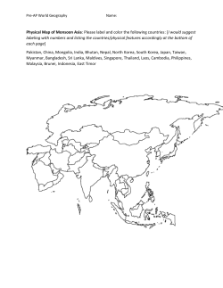


© Copyright 2026