1. health and fitness

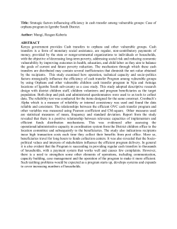
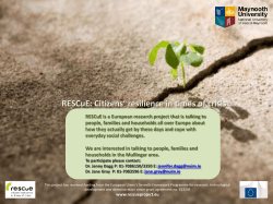
GDS Working Paper
2015-5
The Effects of Community Income Inequality on
Health: Evidence from a Randomized Control Trial
in the Bolivian Amazon
Eduardo A. Undurragaa,*, Jere R. Behrmanb, William R. Leonardc,
Ricardo A. Godoya
The GDS Working Paper series seeks to share the findings of the Center’s ongoing research in order to contribute
to a global dialogue on critical issues in development. The findings may be preliminary and subject to revision as
research continues. The analysis and findings in the papers are those of the authors and do not necessarily
represent the views of the Center for Global Development and Sustainability, the Heller School for Social Policy
and Management or those of Brandeis University.
Center for Global Development and Sustainability
The Effects of Community Income Inequality on Health: Evidence from a
Randomized Control Trial in the Bolivian Amazon
Eduardo A. Undurragaa,*, Jere R. Behrmanb, William R. Leonardc, Ricardo A. Godoya
Abstract
Research suggests that poorer people have worse health than the better-off and, more
controversially, that income inequality harms health. But findings suffer from endogeneity. We
addressed the gap by using a randomized control trial among a society of forager-farmers in the
Amazon. Treatments included one-time unconditional income transfers to the poorest
households and to all households, with untreated villages as controls. We assessed the effects of
income inequality, absolute income, and spillovers within villages on self-reported health,
objective indicators of health and nutrition, and adults’ substance consumption. Most effects
came from relative income. Targeted transfers increased the perceived stress of participants in
better-off households. Evidence suggests increased work efforts among better-off households
when the lot of the poor improves, possibly due to a preference for rank preservation. Our study
points to paths by which inequality might affect health. We discuss the factors that may have
attenuated the results and implications.
Keywords: health | economic inequality | development | social epidemiology | income transfers
JEL: C93, I14, I15, I38, Z13
Word count: 6,962 words, Tables: 6, Figures: 2
a
Heller School for Social Policy and Management, Brandeis University, MS035, 415 South
Street, Waltham, MA 02454-9110, USA; [email protected]; [email protected].
b
Department of Economics, Sociology, and Population Studies Center, University of
Pennsylvania, 3718 Locust Walk, Philadelphia, PA 19104-6297, USA;
[email protected].
e
Department of Anthropology, Northwestern University, 1810 Hinman Avenue, Evanston, Ill
60208-1310, USA; [email protected].
*
Corresponding author. Heller School for Social Policy and Management, Brandeis University, MS035,
415 South Street, Waltham, MA 02454-9110. Telephone: +1 781 736-3954, [email protected].
1
1. Introduction
Researchers from various disciplines have long shown that poorer people have worst health
than richer people. But in the past two decades research has highlighted the perceived harm of
income inequality on individual health (Wilkinson and Pickett 2009). Why this might happen is a
debate in progress. The mechanisms that better seem to explain the relation between community
income inequality and individual health are: (i) inequalities in absolute income or material living
standards and (ii) psychosocial and behavioral mechanisms that affect health (Lynch, et al.
2000).
The absolute income approach focuses on the impact of material deprivation, access to
healthcare, and poor nutrition and sanitation on health. Income inequality leads to an
underinvestment in various areas, including infrastructure, health services, and insurance, which
affect mainly the poor (Smith 1996; Lynch, et al. 2000). If so, we would expect a non-linear
effect of income on health, with a decreasing effect as income increases. Material deprivation
harms health and nutritional status, but the effect of income inequality on health is still unclear
(Deaton 2003; 2013).
Other researchers stress the psychosocial paths by which income inequality might affect
health, the relative income hypothesis. Having lived and evolved during a broad swath of history
in largely egalitarian hunter-gatherer societies with reciprocity norms, significant inequities
might undermine health through psychosocial stress from social comparisons (Wilkinson 2000).
Psychosocial stress is partly determined by economic inequality, and researchers have identified
several biological mechanisms through which stress affects health (Brunner 1997; Marmot, et al.
1999). Most of the literature on the relative income hypothesis suggests that income inequality
produces psychosocial stress by the erosion of social capital and cohesion, which in turn affects
individual health and nutritional status (Kawachi and Kennedy 2002; Wilkinson and Pickett
2009).
Despite great interest in the effects of income inequality on health, studies so far have relied
on observational data, and thus are limited by endogeneity biases. Using a randomized control
trial (RCT) among a society of forager-farmers in the Bolivian Amazon, the Tsimane’, we
examine the effects of absolute income and community income inequality on several indicators
2
of individual health. Randomization occurred at the village level, and all households in a total of
40 treated and control villages were surveyed. In addition to assessing the direct effects of the
treatments, we assessed their spillovers. If targeted income transfers impact a community,
overlooking spillover effects within a community would result in an underestimation of the
effects of the transfers or in the unwarranted conclusion that health improvements took place
from a decrease in inequality. 1
The debate about absolute and relative income effects on health matters because of its policy
implications. If worse health results mainly from deprivation, improving health may require
policies targeted at the poor through, for example, income transfers. If, instead, worse health
results mainly from the distribution of income, then income-related policies to improve health
should focus on income redistribution. Our study design has at least two advantages. First, the
small scale of villages and occupational homogeneity allowed us to rule out confounders such as
ethnicity, residential segregation, healthcare coverage or health investments, differential
exposure to pollution, and large differences in occupation and lifestyle when examining the
effects of community income inequality on health. Second, randomizing the treatment across
villages allows us to both remove endogeneity biases and estimate the impact of transfers on the
entire village economy.
2. The people
Tsimane’ are a tightly-knit endogamic society of forager-farmers living in the tropical rain
forest of the department of Beni, Bolivia, mostly along the rivers Maniqui and Apere. Recent
estimates by the Tsimane’ Council –the main governing body of the Tsimane’– suggest they
number about 14,200 individuals, living in about 95 villages of at least eight households. A
typical Tsimane’ village has about 20 households (standard deviation, SD=24) with an average
of six people per household. Despite occasional contact with Europeans since the sixteenth
1
Recent research on conditional income transfers in Mexico suggests that treatments may have
substantial spillover effects within the community (Angelucci and De Giorgi 2009; Bobonis and Finan
2009). However, to our knowledge, spillover effects have been examined only in one study for
unconditional income transfers (Haushofer and Shapiro 2013), with negligible effects (in Kenya).
3
century, the Tsimane’ remained relatively isolated until Protestant missionaries settled in the
region in the 1950s and until the building of roads during the 1970s, which facilitated
encroachment by cattle ranchers, logging firms, and highland farmers.
Tsimane’ are economically self-sufficient, with limited market exposure. Subsistence
centers on hunting, fishing, plant foraging, and slash-and-burn agriculture, with the sale of thatch
palm and cash cropping of rice and plantains becoming increasingly important. In a world-wide
comparative study of 15 small-scale rural societies, Tsimane’ ranked next to lowest in market
exposure, with about seven percent of households’ food energy consumption purchased in the
market (Henrich, et al. 2010). Another study (1999-2000) found that goods bought in the market
accounted for less than three percent of the value of household consumption, and only 2.5
percent of goods came from outside the village (Godoy, et al. 2004). Previous studies suggest
that the Tsimane’ have low wealth inequality and that economic rank is relatively static
(Undurraga, et al. 2010).
As is true of other native Amazonian societies, Tsimane’ have norms of extensive sharing
and reciprocity. Tsimane’ borrow each other’s assets frequently, often without asking the owner,
share a home-fermented beverage (chicha), and work communally, particularly in smaller
villages (Godoy, et al. 2004). The Tsimane’ language does not include a word for stress, and a
recent study suggests that Tsimane’ adults have one of the lowest reported cortisol
concentrations – a stress-related biomarker – in any population-based study (Nyberg 2011).
A substantial share (33-40%) of Tsimane’ children are growth-stunted (Foster, et al. 2005;
Godoy, et al. 2010), and have low hemoglobin levels (Lindsay, et al. 2003). However, a study by
Godoy, et al. (2005) suggests that the Tsimane’ diet meets daily energy and protein
requirements, so child-stunting is probably explained by high infectious disease loads. Tsimane’
men of higher social status have better nutritional indicators than men of lower status (ReyesGarcía, et al. 2008) and parental wealth is positively associated with children’s nutritional status
(Godoy, et al. 2006), providing partial support to the absolute income hypothesis (albeit with the
usual caveats about endogeneity). Inequality may affect nutritional status through the relative
ability of high social status individuals to gain preferential access to resources (Patton 2005;
Reyes-García, et al. 2009). While the average Tsimane’ body mass index has increased over
4
recent years, Tsimane’ are not experiencing increased obesity as one might expect due to
ongoing acculturation and increases in income (Zeng, et al. 2013a).
Recent studies of blood pressure among Tsimane’ adults suggest that their blood pressure is
slightly above other native Amazonian societies, but lower than blood pressure in other
developing countries (Gurven, et al. 2012; Zeng, et al. 2013b). These studies have estimated that
between four to six percent of Tsimane’ have hypertension with minor or no differences by
gender.
3. Experimental design and methods
3.1
Data, sample, and treatments
We used a unique dataset from a RCT that permits assessment of the effects of a one-time
unconditional in-kind income transfer on various indicators of individual well-being, including
health, nutrition, income, wealth, and human capital. The trial had two treatments (Figure 1). In
treatment 1 (T 1 ) all households in the village received the transfer and in treatment 2 (T 2 ) only
the poorest 20% of households in a village received the transfer. Households in the top 80% of
the income distribution in T 2 villages, and all households in the control villages received
improved rice seeds. 2 Randomization was done at the village level to assess the impact of
transfers on the entire local economy, rather than only on treated households.
2
Public-use data from the RCT are available at http://heller.brandeis.edu/academic/sid/tsimane/;
[email protected].
5
Figure 1.
Summary of the experimental design
NOTE. – HH denotes household. All households in T 1 received rice transfers; only the households
in the bottom 20% of the village income distribution in T 2 received income transfers, and the
top 80% received rice seeds; all households in the control group received rice seeds. The
recipient of the transfers was chosen at random between the male and female household head
in all groups. The baseline sample included 3,449 individuals in 563 HH.
The trial included 40 Tsimane’ villages and was informed by a panel study (2002-2010) and
almost two decades of ethnographic work among the Tsimane’ (Figure 2). To select the sample
of villages for the trial, we eliminated villages that were participating in others studies, were too
small, were too costly to reach, or contained other ethnic groups. The inclusion criteria left 65
villages of which we selected the 40 villages for the trial based on accessibility and safety (e.g.,
6
unsafe owing to the presence of illegal loggers, or required carrying large amounts of rice in
canoes up shallow rivers).
Figure 2. Map showing the study area and the distribution of Tsimane’ villages in the panel
survey (Department of Beni, Bolivia)
NOTE. – The colors of the territory denote elevation; mamsl denotes meters above mean sea
level. The square symbols and letters in each town are approximately proportional in size to town
population. Panel shows the 13 villages that were included in the TAPS panel study (2002-2010).
RCT denotes randomized control trial; the black dots show the 40 villages that were included in
the trial. Tsimane’ territory is an administrative division that does not necessarily reflect the lands
inhabited by the Tsimane’.
7
We conducted a baseline survey from February to May 2008, gave the transfers between
October 2008 and January 2009, and conducted a follow-up survey between February and May
2009. We collected demographic, anthropometric, and self-reported health data from all
household members (or their parents in the case of children <16 years old), but limited collection
of other data to adults (≥16 years old or younger if they headed a household). The sample
included 3,449 individuals in 563 households. About one-fifth of the sample had left by the time
of the follow-up survey. We did not track those not present due to budget limitations, but tested
for attrition bias in the robustness analysis. The final sample included 494 households and 2,555
people with repeated measures.
We did not use cash transfers because of the limited use of money among the Tsimane’ in
isolated villages. Instead, we used edible rice as in-kind income because rice is their main cash
crop (Vadez, et al. 2004), and a proxy for cash that is both fungible and consumable.
Treatment 1 (T 1 ): 782 kg of edible rice were allocated to each of the 13 randomly-chosen
villages. The total transfer was equally divided among all households in a village
(mean/household: 58 kg; median: 52 kg; SD: 23 kg; range 30-131 kg). Total rice per person
varied by household size and by the total number of households in a village.
Treatment 2 (T 2 ): 782 kg of rice were allocated to another 13 randomly-chosen villages;
however, the total transfer was equally divided only among the poorest 20% of households in the
village (mean/household: 177 kg; median: 157 kg; SD: 81 kg; range 98-395 kg). Households in
the top 80% of the village income distribution received 5.9 kg of improved rice seeds.
To identify the poorest 20% of households in each village, we used the area of old and
fallow forest cleared by households (adjusted by household size) at baseline. Each household
clears forests annually to plant crops. The total area of forest cleared is a sensible proxy for
annual income because all farm output obtained from the plots is consumed, bartered, or sold;
thus area of forest cleared captures total household annual consumption and monetary income
from farm products. However, the measure has limitations, such as not capturing wage labor or
income from the sale or consumption of forest goods.
Controls: All households in the remaining 14 villages acted as controls, and received 5.9 kg
of improved rice seeds each, the same as obtained by the top 80% of households in T 2 villages.
8
3.2
Significance of transfers
The rice transfers were economically important. The transfers of edible rice were equivalent
to about US$11/person for people in T 1 villages, US$33/person for people in the bottom 20% of
T 2 villages, and US$1.70/person for people in control households. The mean daily monetary
income per person among the Tsimane’ (wage labor + sale of farm and forest products) was
about US$0.90. Hence, transfers amounted to income earned on average over 12.4 days (T 1 ) or
36.5 days (T 2 ). The perceived value of the improved rice seeds at the time of the transfer may
have been even lower, as there was no market for improved rice seeds in the region, and in focus
groups following the trial, we found that Tsimane’ did not like the harvested rice from improved
seeds. 3
The transfers also represented a substantial infusion of energy and protein to households. If
we assumed a10 percent wastage over the duration of the trial, the average rice transfer (T 1 =58
kg, T 2 =177 kg) would have added 1,249 kcal/day and 25 g/day of protein to average household
availabilities in T 1 villages, and 3,813 kcal of energy and 75 grams of protein to average
household availabilities in T 2 villages (Undurraga, et al. 2014).
We asked household heads about the actual use of the transfers during the follow up survey.
Most households did not sell or barter the rice received. Households in T 1 and the bottom 20% of
T 2 reported eating 76% of the edible rice, and 11% of the rice was given as gifts to others. Most
of the improved rice seeds were planted (81%).
3.3
Outcome variables
We examined three types of health-related outcomes: self-reported health, objective
measures of health and nutrition, and substance consumption by adults. For self-reported health,
we examined self-perceived stress and health-status. Objective measures of health and nutrition
included systolic and diastolic blood pressure (SBP, DBP), weight-for-height-Z-score (WHZ),
and percent body fat. Last, we included two measures of traditional substance use, consumption
of chicha and coca. Table 1 contains definitions and summary statistics of the outcome variables.
3
Depending on whether control households decided to plant the improved rice seeds or not, these
transfers may have had a deferred benefit that is comparable to T1 in the amount of rice produced.
9
Table 1. Definition and summary statistics of outcome variables used in the analysis
2009
2008
Definition
Obs.
Mean St. dev.
Obs. Mean St. dev.
Stress
Total episodes of the following negative emotions
during the seven days before the survey:
nervousness, anger, worry, sadness, inability to
sleep, shame, frazzled at not having enough time to
do all the subsistence and household chores needed,
and envy (adults).
1,041
6.91
6.77
1,078
7.96
6.42
Health
Self-reported health status at the time of the survey:
How is your health now? 1: poor or bad; 2: ok or
good; 3: very good (all participants)
2,496
2.04
.40
2,468
2.03
.40
Systolic Average of three measures of systolic blood
pressure [mmHg] (adults ≤60 yrs. old)
883 113.84
11.62
926 114.85
12.01
Diastolic Average of three measures of diastolic blood
pressure [mmHg] (adults ≤60 yrs. old)
883
69.62
8.41
926 69.10
8.68
Difference between weight-for-height value of
Tsimane’ child and median value of reference
population for the same sex and age, divided by the
standard deviation of the reference population
(children between 2 and 16 yrs. old)a
966
.34
.82
Body fat Total weight of fat of the person divided by total
[%]
body weight [%]. The total weight of fat is derived
from the sum of 4 skinfolds using the DurninWomersley equations (adults ≥18 year of age)b
701
22.37
8.42
WHZ
895
.26
.83
755 22.19
8.38
Coca
Indicator variable. 1: participant consumed coca
during the seven days before the day of the
interview (adults)
1,081
.25
.43
1,092
.24
.43
Chicha
Indicator variable. 1: participant consumed chicha
during the seven days before the day of the
interview (adults)
1,081
.34
.47
1,092
.31
.46
NOTE. – We used 16 years of age as the cut off for adults (unless noted) because Tsimane’ typically
set up independent households by that age. The summary variables are limited to participants who were
present during baseline (2008) and follow-up (2009). Variables used in the regressions as controls
included participants’ age (mean: 19.1; standard deviation: 17.89 years) and gender (50.7% males), and
walking distance (hours) from the village to the nearest road or town during the dry season (mean 5.2; St.
Dev.:5.6 hours). a We only included children >2 years of age as Tsimane’ mothers breastfeed their
children for about two years, so including younger children may have increased the age-related
heterogeneity regarding rice consumption by children. b Lactating and pregnant women were excluded
from body fat measurements, and we only included Tsimane’ Tsimane’ ≥18 years of age.
10
Perceived stress captured the self-reported total number of episodes of eight negative
emotions experienced by the participant during the seven days before the interview. We asked a
separate question for each negative emotion, and then summed the total number of episodes. The
questions for these eight emotions were adapted from the Perceived Stress Scale (Cohen,
Kamarck and Mermelstein 1983). We asked children and adults about their current health status,
and measured it on a Likert scale (Idler and Benyamini 1997).
SBP and DBP were defined as the average of three consecutive measures of blood pressure.
Interviewers used an automatic blood pressure monitor, and took three measures of blood
pressure for each adult on the upper left arm using a standard protocol (Pickering, et al. 2005).
Participants rested sitting for at least five minutes before the first measure and a minimum of two
minutes between each measure. We excluded adults >60 years of age from the main analysis on
blood pressure to avoid the influence of older age.
We followed the protocol by Lohman, Roche and Martorell (1988) to measure height and
weight. Percent body fat was estimated from the sum of four skinfolds using the DurninWomersley equations (Durnin and Womersle 1974). Percent body fat indicates relative fitness
and WHZ captures the difference between the measured value of the Tsimane’ child’s WHZ and
the median value of the reference population of the same sex and age (World Health
Organization 2006), with low values of WHZ reflecting acute energy deficiency (i.e., recent food
deprivation or illness). We did not use measures of height-for-age (HAZ, usually used as an
indicator of chronic undernutrition), or weight-for-age (used as an indicator for both chronic and
acute energy deficiency), because we are trying to capture short-term effects of the transfers, and
most Tsimane’ do not keep track of their ages. 4
We used coca and chicha to measure traditional substance use. Though mainly a highland
crop, coca varieties suitable to the lowlands are grown by the Tsimane’. Unlike the highlands,
where coca leaves are consumed for work, leisure, and rituals (Mamani and Carter 1986), among
Tsimane’ coca is essentially consumed when doing hard physical work (e.g., clearing forest
cover for farming). The consumption of coca leaves captures whether the person has had intense
work activities. In contrast, chicha is produced by women at their homes, fermented from a
4
Despite these limitations, which may undermine some of the usefulness of age-standardized Z scores,
we estimated the effects of the transfers on HAZ scores; results were largely consistent with WHZ.
11
variety of locally-grown plants, and is the cornerstone of Tsimane’ social life. It is consumed in
groups and is the preferred way through which Tsimane’ share their experiences with others and
express pro-social behavior. Chicha is an indicator of whether the person has had meaningful
social interactions with other villagers; it proxies for traditional pro-social behavior.
Control variables included baseline (2008) measures of the health outcomes, participant’s
age and gender (male), and walking distance (hrs.) from the village to the nearest town or road
during the dry season.
3.4
Identification strategy
We used the following model to analyze average treatment effects:
Y ihvt = α + β 1 T 1hvt + β 2 T 2hvt + γYear t + δ 1 T 1hvt ∙Year t + δ 2 T 2hvt ∙Year t + υX ihvt + ε ihvt (1)
where the subscripts stand for individual (i), household (h), village (v), and year (t). The outcome
variable, Y ihvt , includes the health outcomes of interest. Year is an indicator variable for time
(year=0 in 2008; year=1 in 2009), and T indicates treatment (T 1 =1 treatment 1; T 2 =1 treatment 2;
T 1 , T 2 =0 control). X ihvt is a vector with the baseline measure of the outcome variable and
controls, and ε ihvt is a disturbance term. δ indicates the average treatment effect (difference-indifference estimator, DID).
We examined the effects of T 1 and T 2 versus control villages at the bottom 20% and top
80% of village income distributions, assuming that there were no spillovers to untreated
households within the same T 2 village (equation 2). We added the term Bot20 to identify
households at the bottom 20% of the village income distribution (Bot20=1 at the bottom 20% of
income distribution at baseline in T 2 village; Bot20=0 otherwise) and a triple interaction term
T 2hvt ∙Year t ∙Bot20 (the coefficient is the triple difference estimator of T 2 ) to equation (1):
Y ihvt = α + (1+Bot20) ∙ (β 1 T 1hvt + β 2 T 2hvt + γYear t + δ 1 T 1hvt ∙Year t + δ 2 T 2hvt ∙Year t ) + υX ihvt + ε ihvt
(2)
12
Last, we used equation (1) to estimate threshold and spillover effects, by comparing the
effects of income transfers on households in the bottom 20% and top 80% of the village income
distribution with equivalent households from control villages. We also analyzed the treatment
effects on different strata of the village income distributions, restricting the sample of
households to the: (i) bottom 20%, (ii) top 80%, (iii) households right above the treatment
boundary of 20% (20%-40%), and (iv) the richest households (top 40%).
4. Results
Baseline balance. We first examined the results from the randomization process (Table 2).
The average health outcomes of participants in T 1 and T 2 villages were largely comparable with
participants in control villages at baseline. The only exceptions were that participants in T 1
villages reported 0.3 (p=.03) fewer episodes of negative emotions (perceived stress) than
participants in control villages, participants in T 2 had 1.96 (p=.04) times higher odds of reporting
very good health compared with their peers in the control group, and participants in T 2 had 3.6%
(p=.04) lower DBP than participants in the control villages at baseline.
Table 2. Baseline differences on health outcomes between participants in treatment (T 1 and T 2 ) and
control villages
Specific.
Stress
Health
SBP
DBP
WHZ
Body fat
Coca
Chicha
NBR
a
OLS
OLS
OLS
OLS
Logit
Logit
OLogit
T1
-.32**
(.145)
1.27
(.352)
-.002
(.013)
.004
(.017)
.04
(.087)
.89
(.637)
.24
(.233)
.17
(.398)
T2
-.24
(.158)
1.96**
(.636)
-.02
(.015)
-.04**
(.017)
-.07
(.088)
-.20
(.618)
.01
(.358)
.28
(.422)
1.58***
(.131)
-2.40***
(.305)
4.68***
(0.011)
4.19***
(0.013)
.07
(.074)
26.40***
(.751)
-4.36***
(.295)
-2.27***
(.388)
1,344
3,288
1,137
1,137
1,198
919
1,424
1,424
Constant
N
NOTES. – All regressions included robust standard errors (in parentheses) adjusted for clustering at the
village level and the following independent variables as controls (coefficients not shown): participant’s age
and gender, and walking distance from the village to the nearest town or road. SBP denotes systolic blood
pressure; DBP: diastolic blood pressure, WHZ: weight-for-height-Z-score. Baseline is a measure of the
outcome variable at baseline (2008). The second row (specif.) shows the regression specification used. NBR
denotes negative binomial; OLogit: ordered logit; OLS: ordinary least squares; Logit: logistic regression.
The coefficients for Ologit and Logit regressions are shown as odds ratios. a The constant term in the
13
ordered logit regressions (health) corresponds to the first cut-point used to differentiate poor or bad health
from good and very good health. The second cut-point (to differentiate bad or good health from very good
health) was 2.59 (standard error: .340).
*** p<.01, ** p<.05, * p<.10
Average treatment effects. We assessed the average treatment effects in T 1 (absolute
income effect) and T 2 (relative income effect) villages, compared with participants in control
villages (Table 3). The results suggest that on average, one-time unconditional in-kind income
transfers to all households in the village (T 1 ) increased the participants’ perceived stress
(reported number of negative emotions) and the consumption of coca, and decreased the
probability of consuming chicha. Participants in villages with income transfers targeted at the
poorest 20% of households (T 2 ) also saw an average increase in perceived stress. On average,
transferring edible rice to all households (T 1 ) and to households in the poorest 20% of the village
income distribution (T 2 ) increased the expected number of reported negative emotions in the
seven days prior to the survey by about 30% (δ 1 =.28, e^δ 1 =1.32, p=.04; δ 2 =0.27, e^δ 2 =1.31,
p=.03). Compared with adults in control villages, adults in T 1 villages had 2.76 (p=.03) times
larger odds of consuming coca and were 3.5 (3.45=1/.29; p=.04) times less likely to consume
chicha.
14
Table 3. Average treatment effects of a one-time unconditional income transfers to all households in
village (T 1 ) and to poorest 20% of households (T 2 ) on health indicators
Specific.
T1
T2
Year
T 1 ∙Year
T 2 ∙Year
Baseline
Constant
N
Stress
Health
SBP
DBP
WHZ
Body fat
Coca
Chicha
NBR
OLogita
OLS
OLS
OLS
OLS
Logit
Logit
-.19***
1.14
.09
.16
.02
.15
1.20
1.15
(.073)
(.225)
(.385)
(.429)
(.027)
(.110)
(.170)
(.271)
-.13
1.44*
-.66
-.85*
-.02
-.05
1.07
1.19
(.081)
(.293)
(.481)
(.445)
(.029)
(.083)
(.223)
(.295)
.25***
1.38
.21
-1.11
-.11**
.14
.61*
1.26
(.077)
(.683)
(.705)
(.851)
(.039)
(.268)
(.172)
(.527)
.28**
.63
-.43
-.96
.01
-.56
2.76**
.29**
(.137)
(.358)
(1.347)
(1.411)
(.074)
(.383)
(1.292)
(.179)
.27**
.40
2.14
2.17
.10
-.05
1.06
.81
(.123)
(.263)
(1.306)
(1.458)
(.067)
(.498)
(.568)
(.485)
.08***
24.64***
.73***
.64***
.70***
.85***
28.41***
21.91***
(.005)
(3.829)
(.018)
(.020)
(.030)
(.017)
(5.74)
(3.675)
1.01***
3.23***
28.41***
22.43***
.03
4.07***
.02***
.08***
(.092)
(.314)
(2.026)
(1.349)
(.039)
(.447)
(.004)
(.023)
2,080
4,908
1,717
1,717
1,861
1,379
2,173
2,173
NOTE. – All regressions included robust standard errors (in parentheses) adjusted for clustering at the
village level and the following independent variables as controls (coefficients not shown): participant’s age
and gender, and walking distance from the village to the nearest town or road. SBP denotes systolic blood
pressure; DBP: diastolic blood pressure, WHZ: weight-for-height-Z-score. Baseline is a measure of the
outcome variable at baseline (2008). The second row (specif.) shows the regression specification used. NBR
denotes negative binomial; OLogit: ordered logit; OLS: ordinary least squares; Logit: logistic regression.
The coefficients for Ologit and Logit regressions are shown as odds ratios. a The constant term in the
ordered logit regressions (health) corresponds to the first cut-point used to differentiate poor or bad health
from good and very good health. The second cut-point (to differentiate bad or good health from very good
health) was 9.39 (standard error: .555).
*** p<.01, ** p<.05, * p<.10
15
Threshold and spillover effects among households in bottom 20% of village income
distribution. In Table 4 we refined the analysis by distinguishing the effects of the unconditional
income transfers on the Tsimane’ living in households at the top 80% of the village income
distribution in T 1 and T 2 villages from those at the bottom 20%, by adding a triple difference
term (T i ·Year·Bot20). The results largely confirm findings in Table 3, but allow some
distinctions. The transfers only affected the perceived stress of participants living in households
at the top 80% of the village income distribution in T 1 and T 2 villages: the transfers increased
their expected number of reported negative emotions in the previous seven days by 35% (δ 1 =.30,
e^δ 1 =1.35, p=.04) and 37% (δ 2 =.31, e^δ 2 =1.37, p=.01) in T 1 and T 2 , compared with participants
in the control group (T 1 : LR χ2=3.59, p=0.17; T 2 : LR χ2=1.52, p=0.47). Also, average increases
in the odds of coca consumption (3.1 times more likely to consume coca than households in
control villages, p=.02) and decreases in the odds of chicha consumption (3.0 times less likely to
consume chicha than households in control villages, p=.08) in T 1 villages only affected those at
the top 80% of the village income distribution. The Tsimane’ living in households that received
the income transfers (bottom 20%) in T 2 villages had .13 (p=.04) times lower odds of reporting
very good health compared with their peers in the control group. Last, we found a 4% (p=.06)
increase in SBP among adults in households at the bottom 20% of the village income distribution
in T 2 villages (using the natural logarithm of SBP for ease of interpretation). Overall, the results
suggest that the transfers had bigger effects on the health of adults in households at the top of the
village income distribution, particularly in T 1 villages. We next analyze the impact of the
treatments by relative income, limiting the sample by quintiles in the income distribution.
16
Table 4. Effects of one-time unconditional income transfers on health outcomes at the bottom 20% and
top 80% of the village income distribution in the two arms of the treatment (T 1 and T 2 ), compared with
control villages.
Specification
Bot20
T1
T2
T 1 ∙Bot20
T 2 ∙Bot20
Year
Year∙Bot20
T 1 ∙Year
T 2 ∙Year
T 1 ∙Year∙Bot20
T 2 ∙Year∙Bot20
Baseline
Constant
N
Stress
Health
SBP
DBP
WHZ
Body fat
Coca
Chicha
NBR
-.01
OLogit
1.20
OLS
.36
OLS
1.24*
OLS
- .04
OLS
- .05
Logit
1.06
Logit
.89
(.071)
- .18**
( .074)
- .17*
( .097)
(.350)
1.19
( .243)
1.40
( .289)
( .431)
.033
( .400)
- .44
( .495)
( .730)
.24
( .448)
- .57
( .457)
( .035)
.02
( .028)
- .03
( .028)
( .188)
.16
( .111)
- .04
( .083)
( .230)
1.12
( .176)
1.02
( .273)
( .227)
1.14
( .274)
1.12
( .302)
- .11
( .149)
.16
( .102)
.76
( .341)
1.05
( .366)
.42
( .777)
-1.06**
( .494)
- .74
(1.198)
-1.84**
( .825)
.03
( .048)
.08
( .052)
- .09
( .242)
.00
( .199)
1.67*
( .503)
1.18
( .449)
1.11
( .422)
1.35
( .495)
.22***
( .083)
.20
( .237)
.30**
( .144)
.31**
( .127)
1.10
( .472)
4.60**
(3.055)
.75
( .402)
.56
( .315)
.59
( .771)
-3.39
(2.307)
- .35
(1.378)
1.37
(1.398)
- .85
( .899)
-2.35
(2.344)
-1.14
(1.387)
1.52
(1.456)
- .10**
( .040)
- .07
( .109)
.01
( .081)
.11
( .083)
.16
( .294)
- .17
( .704)
- .60
( .415)
.08
( .467)
.64
( .202)
.60
( .504)
3.07**
(1.431)
1.21
( .786)
1.13
( .514)
2.40
(1.676)
.33*
( .209)
.89
( .653)
- .21
( .289)
- .27
( .319)
.31
( .325)
.13**
( .132)
- .21
(2.767)
5.02*
(2.629)
1.72
(3.372)
4.01
(2.618)
.04
( .203)
- .03
( .164)
.31
( .811)
- .39
( .848)
.47
( .607)
.74
( .797)
.33
( .374)
.44
( .481)
.08*** 25.11***
(.005)
(3.910)
.73***
( .018)
.64***
( .020)
.70***
(.030)
.85*** 29.13*** 22.06***
(.017)
(6.036)
(3.697)
28.28***
(2.011)
1,717
22.25***
(1.315)
1,717
.03
( .040)
1,861
1.01***
( .092)
2,080
3.26***
(.319)
4,908
4.10***
( .464)
1,379
.02***
(.004)
2,173
.09***
(.024)
2,173
NOTE. – All regressions included robust standard errors (in parentheses) adjusted for clustering at the
village level and the following independent variables as controls (coefficients not shown): participant’s age
and gender, and walking distance from the village to the nearest town or road. SBP denotes systolic blood
pressure; DBP: diastolic blood pressure, WHZ: weight-for-height-Z-score. Baseline is a measure of the
outcome variable at baseline (2008). The second row (specif.) shows the regression specification used. NBR
denotes negative binomial; OLogit: ordered logit; OLS: ordinary least squares; Logit: logistic regression. The
coefficients for Ologit and Logit regressions are shown as odds ratios. The constant term in the ordered logit
regressions (health) corresponds to the first cutpoint used to differentiate poor or bad health from good and
17
very good health. The second cutpoint (to differentiate bad or good health from very good health) was 9.48
(standard error: .570). The coefficient T 2 ·Year·Bot20 is the triple difference estimate of the second treatment,
assuming there are no spillover effects; T 1 ·Year·Bot20 shows the effects of universal transfers on households
at the bottom 20% of the village income distribution.
*** p<.01, ** p<.05, * p<.10.
Treatment effects by income groups. Table 5 shows the average treatment effect on
households in different positions in the village income distribution (by quintiles, Q i ) in T 1 and T 2
villages, compared with equivalent households of the 14 control villages. The rows in Table 5
show the difference-in-difference coefficient, DID (T i *year), for the regression of the different
outcomes for each sub-sample. These coefficients allowed estimating spillover effects for
households in T 2 and absolute income effects for households in T 1 , compared with households in
the control villages. We analyzed the treatment effects for households in each of the following
income groups: (a) the bottom 20% (poorest, Q 1 ), (b) top 80% (Q 2 -Q 5 ), (c) households right
next to the treatment boundary (between the bottom 20% and bottom 40%, Q 2 ), and (d) the
richest 40% of households (Q 4 -Q 5 ) in each village. We first examine the results of universal
unconditional income transfers (T 1 ), and then examine transfers targeted at the poorest
households (T 2 ).
The results in Table 5 confirm that, on average, universal unconditional transfers (T 1 )
significantly increased the perceived stress of adults in households at the top 80% of the village
income distribution, but not among adults in the poorest households (Q 1 ). Adults in households
at the top 80% of the village income distribution (Q 2 -Q 5 ) in T 1 villages reported 1.35 (p=.04)
times more episodes of negative emotions than their peers in control villages. The difference was
more striking among households in Q 2 and Q 4 -Q 5 with 52% (p=.04) and 47% (p=.03) higher
expected number of reported episodes of negative emotions compared with controls. All adults in
T 1 households saw a decrease in their probability of consuming chicha, irrespective of their
position in the village income distribution. The results also suggest that adults in households at
the top 80% of the village income distribution increased their probability of consuming coca.
However, upon further examination, we found that the observed change was mostly driven by a
substantial increase in the probability of consuming coca of adults in Q 2 , who were 11.7 (p<.01)
times more likely to consume coca than their peers in control villages. We ran a regression for
18
Q 3 , and found no significant results: T 1 ∙Year = 1.89, p=.50; regression not shown. Interestingly,
this same group (Q 2 ) saw an average decrease of 1.2 (p=.05) percentage points of body fat,
consistent with the observed increase in physical work associated with the consumption of coca.
Among households in T 2 villages, we found a significant increase in the perceived stress of
adults who did not receive the unconditional income transfers, particularly among those at the
top 40% of the village income distribution (Q 4 -Q 5 ). On average, adults in T 2 villages who did
not receive rice transfers (Q 2 -Q 5 ) increased 1.37 (p=.01) times the expected number of reported
negative emotions (1.42 times for Q 4 -Q 5 households, p=.08) compared with their income peers
in control villages. Children in households at the top 40% of the village income distribution (Q 4 Q 5 ) also saw an average increase of .22 SD (p=.06) in their WHZ. 5 The Tsimane’ living in
households that received the income transfers (bottom 20%) had .10 (p=.08) times lower odds of
reporting very good health compared with their peers in the control group, and the odds of
reporting very good health were even lower for households in Q 2 (.04 times lower than Q 2
controls, p<.01) compared with controls. Adults in the bottom 20% of T 2 villages also had an
average increase of 6% (p=.02) and 8% (p=.06) SBP and DBP, compared with their income
peers in the control group.
5
In a previous analysis we found no effects of the unconditional cash transfers on child’s WHZ indicators
(Undurraga, et al. 2014); however, we only examined direct average effects.
19
Table 5. Effects of the unconditional income transfers on a sample of households on different positions in the village income distribution
(bottom 20%, top 80%, treatment boundary 20%-40%, and richest households) in T 1 and T 2 villages, compared with equivalent households
in control villages.
Quintiles
Q1
DID
Stress
Health
SBP
DBP
WHZ
Body fat
Coca
Chicha
Specific.
NBR
OLogit
OLS
OLS
OLS
OLS
Logit
Logit
T 1 ∙Year
.10
.27
-.56
.58
.04
-.24
1.35
.11*
(.267)
(.311)
(2.679)
(3.582)
(.176)
(.745)
(1.463)
(.133)
.05
.10*
6.37**
5.53*
.08
-.26
.91
.39
(.301)
(.130)
(2.627)
(2.840)
(.137)
(.930)
(.725)
(.339)
.30**
.74
-.35
-1.14
.01
-.60
3.21**
.33*
(.145)
(.410)
(1.377)
(1.386)
(.081)
(.415)
(1.557)
(.209)
.31**
.55
1.37
1.51
.12
.08
1.22
.89
(.127)
(.313)
(1.394)
(1.453)
(.083)
(.467)
(.826)
(.650)
.42**
.85
-.58
-1.19
-.05
-1.24*
11.72***
.14*
(.201)
(.985)
(2.775)
(2.211)
(.160)
(.614)
(9.876)
(.156)
.21
.04***
3.20
1.06
.22
-.76
8.82
.33
(.211)
(.052)
(3.217)
(3.500)
(.135)
(.961)
(12.665)
(.429)
.38**
.41
.67
.03
.03
-.92
2.34
.19***
(.181)
(.379)
(1.990)
(1.553)
(.075)
(.580)
(1.413)
(.113)
.35*
.89
1.70
1.93
.22*
-.59
.67
.71
(.197)
(.885)
(1.543)
(1.577)
(.117)
(.700)
(.486)
(.734)
[Bot. 20%,
poorest]
Q2- Q5
T 2 ∙Year
T 1 ∙Year
[Top 80%]
T 2 ∙Year
Q2
T 1 ∙Year
[Treatment
boundary]
Q4- Q5
T 2 ∙Year
T 1 ∙Year
[Top 40%,
richest]
T 2 ∙Year
NOTE. – Regressions only include the sample of households in the quintile indicated on the left column. All regressions included robust
standard errors (in parentheses) adjusted for clustering at the village level and the following independent variables as controls (coefficients
not shown): participant’s age and gender, and walking distance from the village to the nearest town or road. Regressions included an indicator
variable T 1 and T 2 , year, and outcome at baseline. SBP=systolic blood pressure; DBP=diastolic blood pressure, WHZ=weight-for-height-Zscore. The second row (specif.) shows the regression specification used. NBR=negative binomial; OLogit= ordered logit; OLS=ordinary least
squares; Logit=logistic regression. The coefficients for Ologit and Logit regressions are shown as odds ratios.
*** p<.01, ** p<.05, * p<.10
20
Attrition. To test for attrition bias, we used data from the baseline survey (2008) and
regressed the health outcomes against indicator variables for T 1 , T 2 , attrition (1=person left at
follow-up; 0=otherwise), and interaction terms between treatment and attrition (T 1 ∙attrition;
T 2 ∙attrition) (Table 6). Most interaction terms were not significant at p<.10, which suggests that
attrition was most likely random and did not introduce bias to our estimates, except for the
interaction term between T 2 and perceived stress (p<.01). Attriters in T 2 villages had, on
average, a higher expected number of reported negative emotions (perceived stress) than nonattriters, suggesting that our average reported estimates for stress in T 2 may be underestimated.
The results also suggest that at baseline, attriters had marginally significant lower perceived
stress (p=.07), and were less likely to consume chicha (p=.07) than participants who were
present at baseline and during the follow-up (2009).
To summarize, income transfers increased the perceived stress of participants in households
at the top 80% of the village income distribution in T 1 and T 2 villages (universal and targeted
transfers) compared with control villages, by about the same amount (~30% increase in the
expected number of negative emotions; Table 4). The increase was most marked among the
richest 40% of households (Table 5). In T 1 villages there was an increase in the odds of
consuming coca and a reduction in the odds of consuming chicha (tables 4 and 5). The biggest
increase in the probability of consuming coca came from participants in households right above
the poorest 20%, who also saw an average decrease in their body fat (Table 5). In T 2 villages, in
addition to the average increase in stress of the top 80%, the transfers affected the WHZ of
children only among the richest 40% of households. Tsimane’ in the poorest 20% of households
in T 2 villages saw a decrease in their odds of reporting good health, and an increase in blood
pressure (SBP and DBP).
21
Table 6. Test of attrition bias
Specif.
T1
T2
Attrition
T 1 ∙Att
T 2 ∙Att
Constant
N
Stress
Health
SBP
DBP
WHZ
Body fat
Coca
Chicha
NBR
OLogit
OLS
OLS
OLS
OLS
Logit
Logit
-.35**
1.27
.003
.01
.07
.97
.23
.34
(.169)
(.333)
(.012)
(.016)
(.093)
(.725)
(.238)
(.387)
-.31*
1.65
-.02
-.04*
-.08*
-.25
.11
.44
(.174)
(.496)
(.016)
(.019)
(.090)
(.528)
(.373)
(.401)
-.22*
.85
.01
-.01
-.07
.29
-.48
-.74*
(.121)
(.097)
(.010)
(.012)
(.131)
(.604)
(.378)
(.405)
.22
.65
-.02
-.01
-.10
-.64
.34
-.41
(.248)
(.185)
(.015)
(.021)
(.214)
(1.116)
(.505)
(.589)
.49***
.82
.004
.01
-.05
-.38
.06
-.01
(.160)
(.209)
(.015)
(.016)
(.193)
(.955)
(.433)
(.535)
1.66***
-2.57***
4.68***
4.20***
.10***
26.54***
(.135)
(.267)
(.011)
(.014)
(.082)
(.740)
(.296)
(.393)
1,244
3,050
1,045
1,045
1,112
854
1,320
1,320
4.23*** -2.20***
NOTE. – All regressions included robust standard errors (in parentheses) were adjusted for clustering at
the village level and included the following independent variables as controls (coefficients not shown):
participant’s age and gender, and walking distance from the village to the nearest town or road. SBP denotes
systolic blood pressure; DBP= diastolic blood pressure, WHZ= weight-for-height-Z-score. Att. denotes
attrition. The second row (specif.) shows the regression specification used. NBR denotes negative binomial;
OLogit= ordered logit; OLS= ordinary least squares; Logit= logistic regression. The coefficients for Ologit
and Logit are shown as odds ratios. The constant term in the ordered logit regressions (health) corresponds to
the first cutpoint used to differentiate poor or bad health from good and very good health. The second
cutpoint (to differentiate bad or good health from very good health) was 2.51 (standard error= .308).
*** p<.01, ** p<.05, * p<.10.
22
5. Discussion
Overall, the results suggest that one-time unconditional in-kind income transfers affected
measures of self-reported and objective health and traditional substance consumption mostly
from relative income effects, in accordance with social comparison studies in richer countries.
The relative income effects were bigger for better-off households, which may be indicative of
social comparisons and preference for rank preservation. We also found some evidence for
absolute income effects, mostly related to chicha consumption. We discuss possible
interpretations of the main results and limitations in the analysis.
5.1
Increase in work efforts from social comparison
Contrary to our expectations, one-time unconditional income transfers increased the
perceived stress of the better-off in T 1 and T 2 villages compared with control villages. In
villages where transfers were universal (T 1 ), the increase in stress came with an increase in the
odds of consuming coca, which is usually consumed when doing intense physical work such as
forest clearing, and a reduction in the odds of consuming chicha, an indicator of meaningful
social interactions (tables 4 and 5). Adults who were right above the poorest 20% of households
(Q 2 ) substantially increased their probability of consuming coca, and there is some evidence that
they decreased their body fat, which is also suggestive of an increase in intense physical work
(Table 5). Because the transfers were equally divided among all households in T 1 villages, they
probably represented a bigger change in the well-being of the poorest households than among the
better-off, due to the decreasing marginal utility of income. The evidence is suggestive of an
increase in work efforts of the better-off, probably as a result of social comparisons.
In villages were transfers were targeted only to the poorest 20% (T 2 ), the transfers did not
significantly change the odds of working harder or engaging in more social behavior, as shown
through the consumption of coca or chicha; however, there is some evidence that the transfers
increased children’s WHZ among the richest 40% of households. Does this reflect an increase in
energy availability for those children from additional work efforts by their parents? A recent
analysis of this RCT by Saidi, et al. (2013), found a significant increase in physical assets and
23
Spanish fluency for better-off adults in households in T 2 villages. Because adult Tsimane’ may
learn Spanish through interactions with outsiders while working in logging camps, cattle ranches,
or farms out of their villages , the relative increase in wealth and Spanish skills is suggestive
evidence that the Tsimane’ in the top 80% of households in T 2 villages also increased their work
efforts.
The robustness analysis showed that income transfers produced, on average, a decrease in
the probability of consuming chicha and an increase in the probability of consuming coca, but
these changes were mostly driven by households at the top of the village income distribution
(tables 4 and 5). We can also rule out that Tsimane’ used the windfall income from the trial to
buy coca, as we would have probably seen a substantial increase in the odds of consuming coca
among the poorest 20% of T 2 , who actually received the biggest transfers of all.
Yet another interpretation is that the increase in the total village food supply simply led to a
temporary, more efficient reallocation of work, substituting farming and foraging activities with
cash-income work such as described above. This effort reallocation could explain the overall
increase in coca consumption and, if cash-income work provided less leisure hours, the decrease
in chicha consumption in T 1 villages. However, while this may have been the case for some
households, the reallocation of effort from agriculture to cash-income work would not explain
the differences observed between households at the bottom 20% of the village income
distribution and those at the top 80% in T 1 villages.
These results present a puzzle: why would social comparisons be so important in a tightlyknit society? It is sensible to think that an increase in income of an anonymous neighbor might
trigger negative emotions and greater work effort, but in a highly endogamic society with strong
rules of preferential cross-cousin marriage, why would an increase in income of one’s kin trigger
similar reactions?
Tsimane’ social norms and settlement patterns may give some clues. Tsimane’ have various
norms of sharing and reciprocity; however, while households share food when stocks dwindle,
they also have a less generous side. Tsimane’ are more likely to share traditional assets than
assets acquired in the market (e.g., metal tools), are less likely to share raw than cooked food,
and may turn their backs while eating to avoid sharing (Ellis 1996). Several travelers have noted
Tsimane’ stinginess with food as far back as the nineteenth century (Balzan 1893; Nordenskiöld
24
2003 [1922]). Traditional Tsimane’ communities consisted in small clusters of rarely more than
five blood-related households settled next to rivers. However, since the 1980s, largely due to the
influence of missionaries and the lure of schools and income-generating activities, these
communities have been replaced by semi-nuclear communities of about three to eight extended
families living together, commonly near a school. Each extended (marriage or blood-related)
family settles around a common patio, but extended families may not necessarily have kinship
bonds between them. If social comparisons occur more intensively between extended families
within a village, then our findings should come as no surprise.
In sum, the evidence suggests that the income transfers increased perceived stress among the
richest households in both scenarios, universal and targeted income transfers. The increase in
stress, together with an increase in the consumption of coca and a decrease in the consumption
of chicha among better off households in T 1 villages, and an increase in wealth and Spanish
fluency among the better-off households in T 2 villages (Saidi, et al. 2013), is suggestive of an
intensification of the work efforts of the richest households. These findings highlight the
importance of social comparisons and relative income, in line with conclusions from previous
studies (Ferrer-i-Carbonell 2005; Luttmer 2005).
5.2
Reduction in stress from transfers
Do these results suggest that the transfers had no absolute income effects on health?
Probably not. If interventions increased everyone’s stress in T 1 and T 2 villages, the poorest 20%
of households might have seen their stress reduced by the transfers to a level that was
undistinguishable from baseline. In T 2 villages transfers might have affected only adults in
households at the bottom 20% of the village income distribution. Likewise, the transfers might
have affected only adults in households at the bottom of the village income distribution in T 1
villages due to the decreasing marginal utility of income, which hints at the absolute income
hypothesis. This interpretation of the observed changes in stress is in agreement with the results
from a recent RCT in Kenya (Haushofer and Shapiro 2013) that gave much bigger (US$404US$1,520) unconditional income transfers to households and, not surprisingly, found that
25
income transfers decreased participants’ stress, with larger effects for bigger transfers (the Kenya
trial also used an objective measure of stress based on the collection of stress hormone cortisol).
5.3
Other explanations and pending questions
There is also an ethnographic interpretation for the increase in perceived stress among the
richest households in T 2 villages. If in a closely-knit and relatively egalitarian society people in
the same village do not think of themselves as having more or less income, they may have
interpreted the transfers as an increase rather than a decrease in inequality. However, the fact that
we also found an increase in stress among adults in households at the top 80% and, more
intensely, among adults in households at the top 40% of the village income distribution in T 1
villages, suggests that social comparisons and preferences for rank preservation are the most
likely mechanism to explain the observed effects.
Surprisingly, unconditional transfers had negative absolute income effects on health.
Tsimane’ who received the transfers in T 2 villages (the poorest 20% of households) saw a
significant decrease in their odds of reporting good health, and an increase in blood pressure
(SBP and DBP). Recent analysis of this trial showed that these households at the bottom of the
income distribution in T 2 villages saw a large increase in wealth and monetary income, but saw
no increase in Spanish skills (Saidi, et al. 2013). These results, in addition to the non-significant
changes we observed in the probability of consuming coca or chicha among adults in this group,
suggest that the observed negative effect on health could have been caused by a more sedentary
life and/or from changes in diet, for example, a decrease in dietary quality.
Despite the fact that households reported giving away about 11% of the edible rice received,
we found no direct spillover effects of the income transfers on health (although we found
significant within-village externalities). The sole exception might have been an increase in WHZ
among the children in the richest 40% of households in T 2 ; however, this improvement in child
nutrition most likely resulted from additional work efforts by this group, triggered by social
comparison and a preference for rank conservation among Tsimane’ adults. A recent randomized
trial in Kenya (Haushofer and Shapiro 2013) also examined the effects of unconditional income
26
transfers on non-recipients and found no significant effects, except for an increase in female
empowerment.
The transfers represented a substantial infusion of energy and protein, from a nutritional
standpoint(Undurraga, et al. 2014). However, we saw almost no effects on anthropometric
indicators of nutritional status (WHZ, body fat), as was found for indicators of child nutritional
status (Undurraga, et al. 2014). The impact of the transfers on nutritional status may have been
affected for at least three reasons. First, reciprocity may have diluted the nutritional effect of the
transfers. Each Tsimane’ household maintains its own food, but will cook in an open space and
often eat from a communal pot, sharing cooked food with the extended family. Second, the
Tsimane’ have relatively good indicators of nutritional status (Foster, et al. 2005), and household
analysis suggest that Tsimane’ diet meets daily energy and protein requirements (Godoy, et al.
2005). Last, the income transfers may have mostly increased energy availability at the household
level, but not improved nutritional quality, such as nutrient density.
5.4
Limitations and implications
Our results suggest that unconditional transfers did affect health, albeit not in the direction
expected. This raises questions on whether other transfer schemes would be needed to achieve
desired improvements in health, such as conditionality, transferring money rather than in-kind
income, or using larger or more frequent transfers.
First, several studies suggest that conditional transfers outperform the impact of
unconditional transfers on schooling outcomes (Baird, et al. 2013); we may have seen different
results had we used conditionality related to health in the transfers. But understanding the effects
of unconditional income transfers is important, particularly in relatively poor countries.
Unconditional income transfers are less expensive, less demanding to implement, and, in most
cases, less patronizing than conditional-income transfers (de Brauw and Hoddinott 2011).
A second characteristic that may have attenuated the results was the use of in-kind transfers
instead of monetary income. Hidrobo, et al. (2014) compared the effects of conditional in-kind,
vouchers, or income transfers in food assistance programs in Ecuador. Their study suggests that
while the three conditional transfer schemes improved the quality and quantity of food consumed
27
among urban and peri-urban communities, food transfers resulted in larger increases in calories
and vouchers lead to larger improvements in dietary diversity. But other studies in Mexico have
found no differences in health and nutritional outcomes between cash and in-kind transfers to
households (Skoufias, Unar and González-Cossío 2008; Cunha 2010), as one would expect from
a well-functioning market. Money is of limited use among the Tsimane’, particularly in more
isolated villages, so despite limitations, food-transfers were the most sensible option in our study
design.
A third factor that may have attenuated the results is related to the use of a one-time income
transfer as opposed to a repeated or more continuous transfer. People may treat one-time
windfall income differently than repeated or continuous income (Thaler 1990). If so, a one-time
income transfer may have not significantly changed people’s behavior or resource allocation.
Further, behavior may also be affected differently by a one-time, exogenous income shock
compared with an endogenous, gradual change in relative income.
In sum, our study produced several noteworthy results. First, we found suggestive evidence
of psychosocial paths through which changes in income affect health indicators. The transfers
increased the perceived stress of the richest households, which is indicative of social
comparisons and preferences for rank preservation. Second, we found some support for the
absolute income hypothesis. The results suggest that the transfers seemed to protect only the
poorest households from perceived stress. We found that the biggest income transfers (to
households at the bottom 20% of the village income distribution of T 2 villages) decreased the
probability of reporting good health and increased blood pressure. Third, unlike previous studies
in rural Mexico, we found no evidence of spillover effects from the transfers. While the debate
over whether economic inequality affects health beyond absolute income is far from conclusive,
our study points to paths by which inequality might affect health.
6. Acknowledgments
For support for this research we thank the Eunice Kennedy Shriver National Institute of
Child Health and Human Development (NICHD) Grant 1R21HD050776 entitled “Inequality,
28
social capital and health in Bolivia”. Secondary support also was provided by Grand Challenges
Canada Grant 0072-03 entitled “Saving Brains: Team 1000+ Saving Brains: Economic Impacts
of Poverty-Related Risk Factors During the First 1000 Days for Cognitive Development and
Human Capital.” The study received IRB approval from Northwestern University (IRB project
approval: STU0007) and by the Tsimane’ Council –the governing body of the Tsimane’– before
data collection. The treatments and controls we used in the trial were defined with and approved
by the Tsimane’ Council. Preliminary results of the study were presented at seminars at the
World Bank, MIT, and Brandeis University. We would like to thank seminar participants,
Thomas Shapiro, Peter Kreiner, Eduardo Valenzuela, Abeer Musleh, Belén Unzueta, and Farzad
Saidi for comments on early drafts, and Camila García for assistance in doing the map.
7. References
Angelucci, M., and G. De Giorgi, "Indirect Effects of an Aid Program: How Do Cash Transfers
Affect Ineligibles' Consumption?," American Economic Review, 99 (2009), 486-508.
Baird, S., F. H. G. Ferreira, B. Ozler, and M. Woolcock, "Relative effectiveness of conditional
and unconditional cash transfers for schooling outcomes in developing countries: A systematic
review," Campbell Systematic Reviews, 9 (2013), 1-124.
Balzan, Luigi, De Irupana a Covendo, de Covendo a Reyes. Informes presentados a la Sociedad
Geográfica Italiana (La Paz, Bolivia: Imprenta de la Revolución, 1893).
Bobonis, G. J., and F. Finan, "Neighborhood peer effects in seconday school enrollment
decisions," Review of Economics and Statistics, 91 (2009), 695-716.
Brunner, E., "Socioeconomic determinants of health - Stress and the biology of inequality,"
British Medical Journal, 314 (1997), 1472-1476.
Cohen, S., T. Kamarck, and R. Mermelstein, "A Global Measure of Perceived Stress," Journal of
Health and Social Behavior, 24 (1983), 385-396.
29
Cunha, Jesse M, "Testing Paternalism: Cash versus in-kind trasnfer in rural Mexico," Discussion
Paper Stanford Institute for Economic Policy Research, 09 (2010).
de Brauw, A., and J. Hoddinott, "Must conditional cash transfer programs be conditioned to be
effective? The impact of conditioning transfers on school enrollment in Mexico," Journal of
Development Economics, 96 (2011), 359-370.
Deaton, Angus, "Health, inequality, and economic development," Journal of Economic
Literature, 41 (2003), 113-158.
------, The great escape: Health, wealth, and the origins of inequality (Princeton, NJ: Princeton
University Press, 2013).
Durnin, Jvga, and J. Womersle, "Body Fat Assessed from Total-Body Density and its Estimation
from Skinfold Thickness. Measurements on 481 Men and Women Aged from 16 to 72 Years,"
British Journal of Nutrition, 32 (1974), 77-97.
Ellis, R., "A Taste for Movement. An Exploration of the Social Ethics of the Tsimane' of
Lowland Bolivia," in Department of Anthropology, (St. Andrews, Scotland: St. Andrews
University, 1996).
Ferrer-i-Carbonell, A., "Income and well-being: an empirical analysis of the comparison income
effect," Journal of Public Economics, 89 (2005), 997-1019.
Foster, Z., E. Byron, Victoria Reyes-García, Tomás Huanca, Vincent Vadez, L. Apaza, E. Pérez,
Susan Tanner, Y. Gutiérrez, B. Sandstrom, A. Yakhedts, C. Osborn, Ricardo A. Godoy, and
William R. Leonard, "Physical Growth and Nutritional Status of Tsimane’ Amerindian Children
of Lowland Bolivia," American Journal of Physical Anthropology, 126 (2005), 343-351.
Godoy, Ricardo A., M. Gurven, E. Byron, V. Reyes-Garcia, J. Keough, V. Vadez, D. Wilkie, W.
R. Leonard, L. Apaza, T. Huanca, and E. Perez, "Do markets worsen economic inequalities?
Kuznets in the bush," Human Ecology, 32 (2004), 339-364.
Godoy, Ricardo A., C. Nyberg, D. T. A. Eisenberg, O. Magvanjav, E. Shinnar, W. R. Leonard,
C. Gravlee, V. Reyes-Garcia, T. W. McDade, T. Huanca, S. Tanner, and TAPS Bolivia Study
30
Team, "Short but Catching Up: Statural Growth Among Native Amazonian Bolivian Children,"
American Journal of Human Biology, 22 (2010), 336-347.
Godoy, Ricardo A., V. Reyes-Garcia, E. Byron, W. R. Leonard, and V. Vadez, "The effect of
market economies on the well-being of indigenous peoples and on their use of renewable natural
resources," Annual Review of Anthropology, 34 (2005), 121-138.
Godoy, Ricardo A., V. Reyes-Garcia, T. McDade, S. Tanner, W. R. Leonard, T. Huanca, V.
Vadez, and K. Patel, "Why do mothers favor girls and fathers, boys? A hypothesis and a test of
investment disparity," Human Nature, 17 (2006), 169-189.
Gurven, M., A. D. Blackwell, D. E. Rodriguez, J. Stieglitz, and H. Kaplan, "Does Blood Pressure
Inevitably Rise With Age? Longitudinal Evidence Among Forager-Horticulturalists,"
Hypertension, 60 (2012), 25-33.
Haushofer, J., and J. Shapiro, "Household response to income changes: Evidence from an
unconditional cash transfer program in Kenya," Unpublished Manuscript, JPAL, (2013).
Henrich, J., J. Ensminger, R. McElreath, A. Barr, C. Barrett, A. Bolyanatz, J. C. Cardenas, M.
Gurven, E. Gwako, N. Henrich, C. Lesorogol, F. W. Marlowe, D. Tracer, and J. Ziker, "Markets,
Religion, Community Size, and the Evolution of Fairness and Punishment," Science, 327 (2010),
1480-1484.
Hidrobo, Melissa, John Hoddinott, Amber Peterman, Amy Margolies, and Vanessa Moreira,
"Cash, food, or vouchers? Evidence from a randomized experiment in northern Ecuador,"
Journal of Development Economics, 107 (2014), 144-156.
Idler, E. L., and Y. Benyamini, "Self-rated health and mortality: A review of twenty-seven
community studies," Journal of Health and Social Behavior, 38 (1997), 21-37.
Kawachi, I., and B. P. Kennedy, The Health of Nations. Why Inequality is Harmful to Your
Health. (New York: The Free Press, 2002).
31
Lindsay, K. M., A. Miller, M. O. Aiello, W. R. Leonard, T. W. McDade, R. A. Godoy, V. ReyesGarcia, V. Vadez, and T. Huanca, "Variation in hemoglobin levels and rates of anemia among
the Tsimane of lowland Bolivia," American Journal of Human Biology, 15 (2003), 45.
Lohman, T.G., A.F. Roche, and R. Martorell, Anthropometric Standardization Reference Manual
Abridge ed. (Champaign, Illinois: Human Kinetics Books, 1988).
Luttmer, E. F. P., "Neighbors as negatives: Relative earnings and well-being," Quarterly Journal
of Economics, 120 (2005), 963-1002.
Lynch, J. W., G. D. Smith, G. A. Kaplan, and J. S. House, "Income inequality and mortality:
importance to health of individual income, psychosocial environment, or material conditions,"
British Medical Journal, 320 (2000), 1200-1204.
Mamani, Mauricio, and William E. Carter, Coca en Bolivia (La Paz, Bolivia: Editorial Juventud,
1986).
Marmot, Michael, Bruce S. Mcewen, Nancy E. Adler, and Judith Stewart, Socioeconomic Status
and Health in Industrial Nations: Social, Psychosocial, and Biological Pathways (New York:
New York Academy of Sciences, 1999).
Nordenskiöld, E., Indios y blancos en el nordeste de Bolivia (La Paz, Bolivia: Plural Editores,
2003 [1922]).
Nyberg, Colleen H., "Diurnal cortisol rhythms in Tsimane' Amazonian foragers: New insights
into ecological HPA axis research," Psychoneuroendocrinology, In Press (2011).
Patton, J. Q., "Meat sharing for coalitional support," Evolution and Human Behavior, 26 (2005),
137-157.
Pickering, T. G., J. E. Hall, L. J. Appel, B. E. Falkner, J. Graves, M. N. Hill, D. W. Jones, T.
Kurtz, S. G. Sheps, and E. J. Roccella, "Recommendations for blood pressure measurement in
humans and experimental animals - Part 1: Blood pressure measurement in humans - A statement
for professionals from the Subcommittee of Professional and Public Education of the American
32
Heart Association Council on High Blood Pressure Research," Hypertension, 45 (2005), 142161.
Reyes-García, Victoria, T. W. McDade, J. L. Molina, W. R. Leonard, S. N. Tanner, T. Huanca,
and R. Godoy, "Social rank and adult male nutritional status: Evidence of the social gradient in
health from a foraging-farming society," Social Science & Medicine, 67 (2008), 2107-2115.
Reyes-García, Victoria, J. L. Molina, T. W. McDade, S. N. Tanner, T. Huanca, and W. R.
Leonard, "Inequality in social rank and adult nutritional status: Evidence from a small-scale
society in the Bolivian Amazon," Social Science & Medicine, 69 (2009), 571-578.
Saidi, Farzad, J. R. Behrman, Eduardo A. Undurraga, and R. A. Godoy, "Inequality, Relative
Income, and Development: Field-Experimental Evidence from the Bolivian Amazon," TAPS
Working Paper Series, 78 (2013).
Skoufias, Emmanuel, Mishel Unar, and Teresa González-Cossío, "The impacts of cash and inkind transfers on consumption and labor supply: experimental evidence from rural Mexico,"
World Bank Policy Research Working Paper, 27 (2008).
Smith, G. D., "Income inequality and mortality: Why are they related? Income inequality goes
hand in hand with underinvestment in human resources," British Medical Journal, 312 (1996),
987-988.
Thaler, R. H., "Anomalies - Saving, Fungibility, and Mental Accounts," Journal of Economic
Perspectives, 4 (1990), 193-205.
Undurraga, Eduardo A., C. Nyberg, D. T. A. Eisenberg, O. Magvanjav, V. Reyes-Garcia, T.
Huanca, W. R. Leonard, T. W. McDade, S. Tanner, V. Vadez, R. Godoy, and Taps Bolivia Study
Team, "Individual Wealth Rank, Community Wealth Inequality, and Self-Reported Adult Poor
Health: A Test of Hypotheses with Panel Data (2002-2006) from Native Amazonians, Bolivia,"
Medical Anthropology Quarterly, 24 (2010), 522-548.
Undurraga, Eduardo A., Ariela Zycherman, Julie Yiu, Jere R Behrman, William R Leonard, and
Ricardo A Godoy, "Gender targeting of unconditional income transfers and child nutritional
33
status: Experimental evidence from the Bolivian Amazon," GCC Working Paper Series, 14-03
(2014).
Vadez, V., V. Reyes-Garcia, R. A. Godoy, V. L. Apaza, E. Byron, T. Huanca, W. R. Leonard, E.
Perez, and D. Wilkie, "Does integration to the market threaten agricultural diversity? Panel and
cross-sectional data from a horticultural-foraging society in the Bolivian Amazon," Human
Ecology, 32 (2004), 635-646.
Wilkinson, R. G., Mind the Gap: Hierarchies, Health, and Human Evolution (London:
Weidenfeld and Nicolson, 2000).
Wilkinson, R. G., and K. E. Pickett, The Spirit Level: Why Greater Equality Makes Societies
Stronger (New York: Bloomsbury Press 2009).
World Health Organization, WHO Child Growth Standards: Length/height-for-age, weight-forage, weight-for-length, weight-for-height and body mass index-for-age. Methods and
development (Geneva, Switzerland: Multicentre Growth Reference Study Group, World Health
Organization, 2006).
Zeng, Wu, D.T.A. Eisenberg, Karla Rubio, Eduardo A. Undurraga, Colleen Nyberg, Susan
Tanner, Victoria Reyes-Garcia, William R. Leonard, Juliana Castaño, Tomas Huanca, Thomas
W. McDade, TAPS Bolivia Study Team, and Ricardo A. Godoy, "Adult Obesity: Panel Study
from Native Amazonians," Economics & Human Biology, 11 (2013a), 227-235.
Zeng, Wu, Eduardo A. Undurraga, Colleen Nyberg, Dan T. A. Eisenberg, Sabita Parida, Ariela
Zycherman, Oyunbileg Magvanjav, Victoria Reyes-García, Susan Tanner, and Ricardo Godoy,
"Sibling composition during childhood and adult blood pressure among native Amazonians in
Bolivia," Economics & Human Biology, 11 (2013b), 391-400.
34