histoneHMM (Version 1.4)
Matthias Heinig
April 2, 2015
1
Example workflow using data included in the
package
Load the package
> library(histoneHMM)
Load the example data set
> data(rat.H3K27me3)
First we analyse both samples separately using the new high-level interface
> posterior = run.univariate.hmm("BN_H3K27me3.txt", data=BN, n.expr.bins=5,
+
em=TRUE, chrom="chr19", maxq=1-1e-3, redo=F)
This call also produces a number of files holding the parameter estimates
and posterior probabilities. We can now load the fit from the file and inspect
its quality visually.
> n = load("BN_H3K27me3-zinba-params-em.RData")
> zinba.mix = get(n)
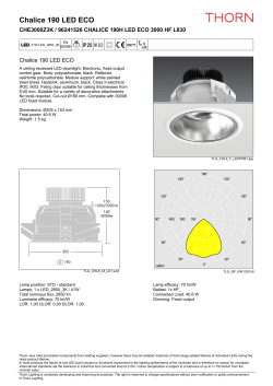
For the visualization we ignore the long tail of the distribution, otherwise it
is difficult to see.
> max = 100
> x = BN[BN[,"chrom"] == "chr19","signal"]
> x[x > max] = NA
Visualize the fit
> plotDensity(model=zinba.mix, x=x, xlim=c(0, max), add=FALSE,
+
col="black", alpha=1)
1
0.14
0.12
0.10
0.08
0.06
0.04
0.02
0.00
0
20
40
60
80
100
Analysis of the second sample is carried out analogously.
>
+
>
>
>
>
>
>
>
>
>
+
posterior = run.univariate.hmm("SHR_H3K27me3.txt", data=SHR, n.expr.bins=5,
em=TRUE, chrom="chr19", maxq=1-1e-3, redo=F)
## load the fit from the file
n = load("BN_H3K27me3-zinba-params-em.RData")
zinba.mix = get(n)
## for the visualization we ignore the long tail of the distribution
max = 100
x = SHR[SHR[,"chrom"] == "chr19","signal"]
x[x > max] = NA
## visualize the fit
plotDensity(model=zinba.mix, x=x, xlim=c(0, max), add=FALSE,
col="black", alpha=1)
2
0.15
0.10
0.05
0.00
0
20
40
60
80
100
After validating both fits we continue with the bivariate analysis
> bivariate.posterior = run.bivariate.hmm("BN_H3K27me3.txt", "SHR_H3K27me3.txt",
+
outdir="BN_vs_SHR_H3K27me3/", data1=BN, data2=SHR,
+
sample1="BN", sample2="SHR", n.expr.bins=5, maxq=1-1e-3,
+
em=TRUE, chrom="chr19")
initialize:$size
[,1]
[1,] 1.705324
$mu
[,1]
[1,] 122.2396
$beta
[1] 0.001918775
initialize:$size
[,1]
[1,] 1.638623
$mu
[,1]
[1,] 130.7187
3
$beta
[1] 0.002098567
initialize:$size
[,1]
[1,] 1.296773
$mu
[,1]
[1,] 16.54621
$beta
[1] 0.1960098
initialize:$size
[,1]
[1,] 1.194342
$mu
[,1]
[1,] 16.99791
$beta
[1] 0.2067472
chr19
chr20
>
>
>
>
>
>
2
## call regions
BN.regions = callRegions(bivariate.posterior, 0.5, "BN", NULL)
# GR2gff(BN.regions, "BN_vs_SHR_H3K27me3/BN_specific.gff")
SHR.regions = callRegions(bivariate.posterior, 0.5, "SHR", NULL)
# GR2gff(SHR.regions, "BN_vs_SHR_H3K27me3/SHR_specific.gff")
Preprocessing data from bam files
histoneHMM works on the read counts from equally sized bins over the
genome. Optionally, gene expression data can be used to guide the parameter
estimation. Here we show how the data is preprocessed. In order to get the full
information we need a bam file containing the aligned ChIP-seq reads, a table of
gene expression values, the lengths of the chromosomes and a gene annotation.
On our website we provide example data that can be downloaded for this
example:
4
>
>
>
>
>
system("wget
system("wget
system("wget
system("wget
system("wget
http://histonehmm.molgen.mpg.de/data/expression.txt")
http://histonehmm.molgen.mpg.de/data/BN.bam")
http://histonehmm.molgen.mpg.de/data/BN.bam.bai")
http://histonehmm.molgen.mpg.de/data/chroms.txt")
http://histonehmm.molgen.mpg.de/data/ensembl59-genes.gff")
Load the expression data. In this experiment we have 5 replicates of each
strain, so we take the mean expression values.
> expr = read.csv("expression.txt", sep="\t")
> mean.expr = apply(expr[,1:5], 1, mean)
The genome object that we pass to the function needs to provide a seqlengths
function, we can use either the BSGenome packages from bioconductor, or simply create GRanges.
>
>
>
>
chroms = read.table("chroms.txt", stringsAsFactors=FALSE)
sl = chroms[,2]
names(sl) = chroms[,1]
genome = GRanges(seqlengths=sl)
Load the gene coordinates such that we can assign the expression values of
a gene to all bins that overlap the gene.
> genes = gff2GR("ensembl59-genes.gff", "ID")
> data = preprocess.for.hmm("BN.bam", genes, bin.size=1000, genome,
+
expr=mean.expr, chr=c("chr19", "chr20"))
> write.table(data, "BN.txt", sep="\t", quote=F, row.names=F)
5