Download Report

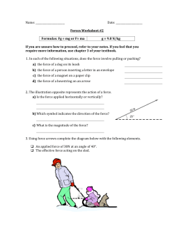
Modeling a Rocket in Orbit Around the Earth
Miroslav P. Zvyagelskiy & Kieran Cunningham
Flathead Valley Community College
May 12, 2015
Abstract
Modeling the path of a rocket-propelled body that is launched from Earth into
a stable orbit requires the derivation of several dynamical systems, as well as
Newton’s second law of motion. The result is several systems of non-linear
differential equations that require a numerical solver such as MATLAB’s ode45
to generate data that can be quantitatively examined and graphically displayed.
Contents
1 Introduction
1.1 Assumptions . . . . . . . . . . . . . . . . . . . . . . . . . . . . .
2
3
2 Derivation
2.1 Define Variables
. . . . . . . . . . . . . . . . . . . . . . . . . . .
4
7
3 Data
3.1 Results . . . . . . . . . . . . . . . . . . . . . . . . . . . . . . . . .
8
8
4 Conclusion
10
5 Equation Appendix
11
6 Bibliography
12
1
1
Introduction
An accurate workable model for launching a rocket from any point on Earth’s
surface into orbit around the Earth is dependent on hundreds of different variables. In order to simplify the situation to fit within the scope of Ordinary
Differential Equations (ODE’s) and MATLAB’s solving abilities, several assumptions must be made. The model will not, for example, take into account
variations in humidity or air temperature during the initial phase of the rocket’s
flight. The minor variations in gravitational pull due to other celestial bodies
such as the moon will be neglected, as well as minor variations in Earth’s gravitational field. A complete list of assumptions is given in section 1.1.
2
1.1
Assumptions
• Earth is a perfect sphere.
• There are no outside bodies (e.g. the moon) whose gravity could have an
effect on the rocket’s trajectory.
• There is no wind.
• The final orbiting altitude of the rocket will be such that air resistance
can be neglected.
• The mass of the rocket does not affect Earth’s position.
• The rocket engine burns at a constant rate the entire time that it is on.
• The engine stops burning at the instant that the rocket reaches the desired
altitude at the correct orbital velocity.
• Small variations in humidity and things like clouds do not interfere with
the rocket’s path.
• In Newton’s Second Law the time rate change of mass is neglected due to
time constraints.
3
2
Derivation
To accurately model the path of a rocket from the surface of the Earth
it is best to use a polar coordinate system, where R is the distance radially
outward from the center of the Earth, and θ is the angle measured clockwise
from the origin starting from the position of the rocket. To find the acceleration
of an object the force and mass must be known. Because rockets use a masspropellant system, their mass will decrease over the duration of the flight. For
the purposes of this model the rocket engine will be simplified such that it
operates at a constant rate, expelling a constant amount of mass every second
at a constant velocity until it is shut off. The function for the rocket’s mass can
then be written as the equation below.
m = m0 −
dm
t
dt
(1)
Figure 1:
There are three main forces that act on a rocket in flight, as shown in Figure
1. The first is thrust. For this assessment, thrust will be treated as a constant
force that acts in the direction of the rocket’s path. It can be calculated using
Newton’s second law, F = ma, by multiplying the velocity of the gas exiting
the rocket by the rate of mass leaving. The rate at which gas leaves the rocket
is equal to the rate of change of the rocket’s mass, which is a function of time.
4
The exit velocity of the gas is a constant that is determined by engine design
and fuel type, thus the equation for the force acting on the rocket due to thrust
can be written as shown in the following equation:
FT = c
dm
dt
(2)
The second main force acting on a rocket is atmospheric drag. Drag acts in
the opposite direction of the rocket’s motion, and is proportional to the square
of its velocity. The force due to drag can be modeled as shown:
FD =
1 2
ρv ACD
2
(3)
where ρ represents a simplified model of air density as a function of the rocket’s
altitude, and is given by the equation
ρ = ρ0 e−((r−re )∗0.001)
The velocity of an object in polar coordinates can be written as
q
˙ 2 + (rθ)
˙ 2
v = (r)
(4)
(5)
To use this in the drag function, it must be modified to be the equation of
velocity relative to the air in Earth’s atmosphere, as shown below.
r
π 2
v = (r)
˙ 2 + (rθ˙ − r
)
(6)
43200
The 0 A0 term in equation
FD =
1 2
ρv ACD
2
(7)
is a constant that is defined as the area that is acted upon by the force of
air resistance, and CD is the drag coefficient, which depends on the shape of
the rocket and the properties of the materials on its exterior. The last major
force that affects a rocket’s motion is the force of gravity. For the purposes of
this paper gravity will always act in the negative R-direction, towards a pointsource at the center of the Earth. Newton defined the force of gravitational pull
to be proportional to the product of the masses of two objects, and inversely
proportional to the square of the distance between their respective centers of
gravity. Factoring in the gravitational constant G, the force acting on a rocket
near Earth can be modeled using the following equation:
FG =
Gme m(t)
(r)2
5
(8)
Because force and drag act in the direction of the path of a rocket, it is
important to factor in the rocket’s angle of incline relative to Earth’s surface,
which will be given as α. If the rocket starts in the vertical position at 90
degrees and then slowly leans over during its flight until it is moving parallel to
the surface of the Earth; alpha can be written as
α=
π
πt
−
2
2tf
(9)
An objects’ acceleration in polar coordinates can be written as follows:
˙ 2 )er + (2r˙ θ˙ + rθ)e
¨ θ
a = (¨
r − r(θ)
(10)
where er and eθ are unit vectors in the r and θ directions. Combining this
F
, the acceleration of a rocket in r and θ can be written as the two
with a = m
second-order differential equations:
−FG
sin(α)
d2 r
=
+
(FT − FD ) + rθ˙2
dt2
m
m
d2 θ
1 cos(α)
˙
=
(FT − FD ) − 2r˙ θ
dt2
r
m
(11)
(12)
At t = 0, r will equal the radius of the earth. The initial velocity in the
r direction will be zero, and the rocket will be launched from θ = 0. Due to
the rotation of the Earth, the initial velocity in the θ direction can be found by
converting one revolution per day into radians per second.
After the rocket
has expelled all of its fuel and reached its orbiting altitude, a second model must
be created to show the unpowered orbital path. Using the final values of r and
θ, and the rocket’s final velocity from the launch as new initial conditions, a
second model can be derived:
d2 r
−FG
=
+ rθ˙2
dt2
mf
(13)
d2 θ
−2r˙ θ˙
(14)
=
dt2
r
This is much the same as the first one, without the forces of thrust and drag.
Drag is excluded because at the rocket’s final orbital altitude the air is so thin
that the force of drag can be neglected altogether. To maintain a steady orbit,
the force of gravity pulling on the rocket must be equal to the centrifugal force
pushing it outward due to the speed of its rotation. This equality can be shown
as
mf ∗ G ∗ me
(vf )2 ∗ mf
=
(15)
r2
r
where vf is the final velocity of the rocket.
6
2.1
Define Variables
• r = Radial distance from the center of the Earth.
• θ = Angular distance travelled.
• G = Gravitational constant.
• me = Mass of the Earth.
• re = Radius of the Earth.
• H = Desired orbital height from surface of the Earth.
• FG = Gravitational force.
• FT = Force of thrust.
• m = Mass of rocket.
• c = Velocity of gas leaving rocket.
• FD = Force due to drag.
• t = Time in seconds.
• vf = Orbital velocity.
• v = Velocity of the rocket.
• α = Angle of incidence.
• ρ = Air density.
• A = Area affecting drag
• CD = Drag coefficient.
• m0 = Initial mass of rocket.
• mf = Final mass of rocket after all fuel is expelled.
7
3
Data
dm [kg/s]
Mass of Rocket [kg]
Rocket velocity [m/s]
Nozzle velocity [m/s]
Altitude above Earth’s surface [m]
θ
dθ
dt
r
dr
dt
α
3.1
At Launch
-60
32000
0
5500
0
0
0.00007427
6378100
0
π/2
During Orbit
0
800
7586.9925
0
546583.237
0.26888
0.0019564
6924683
0
0
Results
Figure 2: Rocket orbits Earth almost twice in 2.944 hours
8
Figure 3: Rocket crashing into Earth due to orbital decay in 4.1667 hours
Figure 4: Rocket escapes orbit after about 3.139 hours
The difference between the images Figure 2, Figure 3, and Figure 4 was a
˙
change in the 16th decimal place of the initial value of θ.
9
4
Conclusion
Modeling a rocket in a real world situation is extremely complex, however a
simplified model can be produced using the limited capabilities of MATLAB and
numerical solver ode45. The results were relatively accurate, and they seem to
be representative of an actual orbit when compared to the available information
on the trajectory of the International Space Station (ISS). The produced figures
show the extreme degree of accuracy that is required to maintain a stable orbit.
Even when using the highest possible degree of accuracy (the 16th decimal
place), the orbit decayed after a little more than three hours.
10
5
Equation Appendix
FG =
Gme m(t)
(r)2
FD =
1 2
ρv ACD
2
ρ = ρ0 e−((r−re )∗0.001)
dm
t
dt
dm
FT = c
dt
m = m0 −
−FG
sin(α)
d2 r
=
+
(FT − FD ) + rθ˙2
dt2
m
m
d2 θ
1 cos(α)
˙
=
(F
−
F
)
−
2
r
˙
θ
T
D
dt2
r
m
q
˙ 2 + (rθ)
˙ 2
v = (r)
˙ 2 )er + (2r˙ θ˙ + rθ)e
¨ θ
a = (¨
r − r(θ)
α=
r
v=
πt
π
−
2
2tf
(r)
˙ 2 + (rθ˙ − r
π 2
)
43200
d2 r
−FG
=
+ rθ˙2
dt2
mf
d2 θ
−2r˙ θ˙
=
dt2
r
mf ∗ G ∗ me
(vf )2 ∗ mf
=
r2
r
11
6
Bibliography
References
[1] J.Peraire, S. Widnall Lecture L14 - Variable Mass Systems: The Rocket
Equation
http://ocw.mit.edu/courses/aeronautics-and-astronautics/16-07dynamics-fall-2009/lecture-notes/MIT16 07F09 Lec14.pdf
[2] Merian, James L., and L. Glenn Kraige. Engineering Mechanics Dynamics.
7th ed. Hoboken: Wiley
[3] Arnold David, Albert Boggess, and John Polking. Differential Equations
With Boundary Value Problems. 2nd ed. Upper Saddle River: Pearson
Prentice Hall
[4] Don Hickethier
[5] Wikipedia
[6] Special thanks to William Pardis for the model rocket used in Figure 1
12