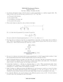
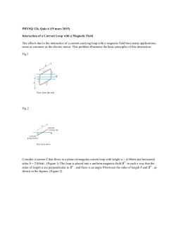
JOURNAL OF APPLIED PHYSICS 117, 163905 (2015)
Tomography based numerical simulation of the demagnetizing field
in soft magnetic composites
S. Arzbacher,1 P. Amann,2 B. Weidenfeller,3 T. Loerting,4 A. Ostermann,5 and J. Petrasch1,a)
1
illwerke vkw Professorship for Energy Efficiency, Vorarlberg University of Applied Sciences,
Hochschulstraße 1, 6850 Dornbirn, Austria
2
Department of Physics, Stockholm University, AlbaNova University Center, 10691 Stockholm, Sweden
3
Institute of Electrochemistry, Clausthal University of Technology, Arnold-Sommerfeld-Straße 6,
38678 Clausthal-Zellerfeld, Germany
4
Institute of Physical Chemistry, University of Innsbruck, Innrain 80-82, 6020 Innsbruck, Austria
5
Department of Mathematics, University of Innsbruck, Technikerstraße 13, 6020 Innsbruck, Austria
(Received 28 January 2015; accepted 2 April 2015; published online 23 April 2015)
The magneto-static behaviour of soft magnetic composites (SMCs) is investigated using tomography based direct numerical simulation. The microgeometry crucially affects the magnetic properties of the composite since a geometry dependent demagnetizing field is established inside the
composite, which lowers the magnetic permeability. We determine the magnetic field information
inside the SMC using direct numerical simulation of the magnetic field based on high resolution
micro-computed tomography data of the SMC’s microstructure as well as artificially generated
data made of statistically homogeneous systems of identical fully penetrable spheres and prolate
spheroids. Quasi-static electromagnetic behaviour and linear material response are assumed. The
3D magnetostatic Maxwell equations are solved using Whitney finite elements. Simulations show
that clustering and percolation behaviour determine the demagnetizing factor of SMCs rather than
the particle shape. The demagnetizing factor correlates with the slope of a 2-point probability function at its origin, which is related to the specific surface area of the SMC. Comparison with experimental results indicates that the relatively low permeability of SMCs cannot be explained by
demagnetizing effects alone and suggests that the permeability of SMC particles has to be orders of
C 2015 AIP Publishing LLC.
magnitude smaller than the bulk permeability of the particle material. V
[http://dx.doi.org/10.1063/1.4917490]
I. INTRODUCTION
Soft magnetic composites (SMCs) are materials made of
ferromagnetic particles mixed with an electrically insulating
binder. Although there are some attempts at using molding
techniques,1 the production process usually involves high
pressure compaction. This is often followed by curing or by
heat treatment if the binder is heat resistant.2,3 The powderlike nature of SMCs results in isotropic ferromagnetic behaviour, which promises more freedom in the design of electrical
devices compared to the anisotropic character of laminated
steel. Additionally, the insulating substrate material prevents
the formation of macroscopic current paths and thus eddy
current losses are small even at high frequencies.4,5 Despite a
generally low permeability and high total core losses at low
frequencies, SMCs are attractive materials for a broad range
of applications in a wide frequency spectrum because of cost
benefits in the production process. These applications include
electric motors, actuators, and sensors as well as induction
heaters, inductors, and even microwave devices.6–10 A thorough understanding of SMCs’ electric and magnetic properties is crucial for manufacturers as well as engineers. The
effect of mixing ratios and constituent particle properties on
the magnetic response of the composite is one of the open
a)
Author to whom correspondence should be addressed. Electronic mail:
[email protected]. Tel.: þ43 5572 792 3801.
0021-8979/2015/117(16)/163905/12/$30.00
questions and has been recently discussed by Anhalt and
Weidenfeller11–13 and others.14–16 Another question of interest is the effect of strain and tension, usually involved in the
production process, on the electromagnetic properties and
was addressed by Hemmati et al.17 and Taghvaei et al.18 for
dense SMCs and Brosseau et al.19,20 for filled polymers.
Several models for heterogeneous magnetic materials
that relate particle permeability, particle shape, and filler
fraction to effective magnetic properties have been developed.21–27 Due to the mathematical analogy of electric permittivity and magnetic permeability in static systems,28 these
models are closely related to the well known models for
electrically heterogeneous materials. These results29–32 also
lead to a better understanding of magnetic phenomena and
vice versa. Ferromagnetic particles repel magnetic fields and
form shape dependent demagnetizing fields, reducing the
particle’s permeability. Thus, in most models, the influence
of particle shape on magnetic properties is accounted for by
demagnetizing factors. This is the magnetic analogy to a
depolarizing field reducing the electric field inside a particle,
which is also often described by the depolarization factor.
For regular geometrical objects, such as ellipsoids, prisms,
or rods, these factors are well known from theoretical or numerical analysis.33–37 In most models of composites, ellipsoids are used to represent any particle shape since they form
homogeneous demagnetizing fields. This results in analytical
expressions mapping particle permeability, demagnetizing
117, 163905-1
C 2015 AIP Publishing LLC
V
[This article is copyrighted as indicated in the article. Reuse of AIP content is subject to the terms at: http://scitation.aip.org/termsconditions. Downloaded to ] IP:
138.232.247.55 On: Fri, 24 Apr 2015 04:32:20
163905-2
Arzbacher et al.
factor, and filler fraction to the corresponding quantities of
the composite.
Although most models do not directly consider magnetic field perturbation in the neighbourhood of particles
caused by their demagnetizing field, a significant fraction of
particles is influenced by their neighbours’ demagnetizing
fields (even in low density SMCs).38–41 Hence, the microstructure complicates modelling and greatly affects
properties like magnetic susceptibility and ferromagnetic
resonance frequency.
The objective of the current work is to determine the
influence of the irregular microstructure of an SMC on the
demagnetizing field represented by the demagnetizing factor.
We use X-ray micro-computed tomography (lCT)42 to
determine the material’s three-dimensional structure. A GE
nanotom-m43 high resolution lCT system capable of voxel
sizes of 1 lm3 and less is used. Subsequently, a 3D unstructured tetrahedral grid is generated using the measured geometry and a tetrahedral mesh generator based on space
indicator functions developed by Friess et al.44 Extensive numerical simulations of the magnetostatic behavior are carried
out using Whitney elements45 as implemented in the open
source finite element method (FEM) software ELMER.46
The numerical simulation provides detailed 3D electromagnetic field information within and outside the SMC, which is
solely based on geometry data and magnetic permeabilities
of individual phases. Hence, the demagnetizing factor can be
investigated independent of non-geometric phenomena, and
experimental uncertainties. The combination of lCT and numerical simulation is referred to as tomography based numerical simulation (TBNS). It has been applied to radiative
transfer,47 conductive heat transfer,48 and fluid flow49 in a
range of different materials. To the best of our knowledge,
this is the first time that TBNS is applied to magnetic phenomena. We used two sample sets, which were experimentally investigated by Anhalt et al.50 For reference, a few
numerical studies on randomly generated data are done and
compared with the results of the sample sets and the already
published numerical work of Mattei and Le Floc’h.25
II. THEORY
A. Vector component volume average
J. Appl. Phys. 117, 163905 (2015)
B. Demagnetizing factor
In a complete magnetic circuit and under the assumption
of linear material response, the magnetic flux density B is
related to an exciting magnetic field H0 via the relative permeability lr
B ¼ l0 ðH0 þ MÞ ¼ l0 lr H0 :
(2)
Thus, for linearly responding material the magnetization M
of the ferromagnetic material is related to the magnetic field
strength H, which is magnetizing the material, by the linear
law
M ¼ vH ¼ ðlr 1Þ H;
(3)
where v denotes the magnetic susceptibility. In noncomplete magnetic circuits, the demagnetizing field HD
reduces the magnetic field inside the ferromagnetic material
and Eq. (2) becomes
B ¼ l0 ðH0 þ M þ HD Þ:
(4)
Due to the microgeometry of SMCs non-complete circuits
have to be considered, even for toroidal cores.
Let us now consider an SMC of regular shape, e.g., an
ellipsoid or a cylinder, completely immersed in a uniform
magnetic field H0 applied along one of the principle directions ek . The orientation in space of the SMC is assumed to
be well defined and fixed. Using the notation introduced in
Subsection II A, the total magnetometric demagnetizing factor Nktot along direction ek is defined34 by
ðHD;k Þm ¼ Nktot ðMk Þm :
(5)
Note that in the case of bulk ellipsoids Nktot is consistent with
the well known demagnetizing factors for ellipsoids but it
also covers non-uniform demagnetizing fields, e.g., in cylinders. The term magnetometric is deduced from magnetometer measurements and will be dropped hereafter. By taking
the vector component volume average Eq. (4) transforms to
ðBk Þm ¼ l0 ½ðH0;k Þm þ ð1 Nktot Þ ðMk Þm :
(6)
Consider an SMC occupying the region V which can be
decomposed into the two disjoint regions V m and V d such
that V ¼ V m [ V d and V m \ V d ¼ ;. The subscripts m and d
refer to the magnetic and dielectric (nonmagnetic) material
phase, respectively. The volume average of the kth vector
component of the vector field v : V 7! R3 on the region V m
is defined by
Ð
vk dV
:
(1)
ðvk Þm :¼ V m
jV m j
In analogy to Eq. (2), an intrinsic permeability lk;m of the
magnetic phase of the SMC is defined by
According to the used standard basis fex ; ey ; ez g subscript k
can either be x, y, or z and will be reserved for that purpose
further on. jV m j denotes the volume of the region V m . This
definition will help to describe the demagnetizing factor in a
concise fashion.
ðMk Þm ¼ ðlr 1Þ ½ðH0;k Þm Nktot ðMk Þm :
ðBk Þm ¼ l0 lk;m ðH0;k Þm :
(7)
This can be understood as the magnetic permeability corrected by the intrinsic demagnetization. Since in noncomplete circuits the magnetic field acting on the material is
H ¼ H0 þ HD volume averaging and Eq. (3) leads to the self
consistent law
(8)
Combining Eqs. (6), (7), and (8) the total demagnetizing factor Nktot (abbreviated with total DMF) of the magnetic material phase becomes
[This article is copyrighted as indicated in the article. Reuse of AIP content is subject to the terms at: http://scitation.aip.org/termsconditions. Downloaded to ] IP:
138.232.247.55 On: Fri, 24 Apr 2015 04:32:20
163905-3
Arzbacher et al.
J. Appl. Phys. 117, 163905 (2015)
Nktot
lr =lk;m 1
;
¼
lr 1
(9)
where lr is the relative permeability of the magnetic bulk
also measured in complete magnetic circuits.51 The only
total DMF of interest in the course of this work will be Nztot .
Therefore, the notation will be simplified by the definition
N tot :¼ Nztot . As mentioned above, not only ring shaped
SMCs but also samples with finite sizes and regular outer
shapes are considered. In order to distinguish the demagnetizing effects caused by the composites’ outer shape from the
demagnetizing effects caused by the inner structure, it is useful to decompose the total DMF into the inner DMF N inn and
the geometric DMF N geo such that
N tot ¼ N inn þ N geo :
(10)
The geometric DMF depends on the external shape of the
SMC alone, while the inner DMF incorporates the SMCs
microstructure. Hence, in bulk material N inn vanishes
almost completely50,52 and N tot is governed by the external
shape of the specimen. On the other hand, N geo vanishes in
toroids, infinitely long cylinders or prisms when their axis
is aligned along the exciting field direction.21 In all other
cases, a geometric demagnetization factor due to free magnetic poles at the surface of the composite, and additionally an inner demagnetization factor due to free poles on
particles and/or agglomerates within the composites
appears.21,25,40 As a result, the permeability of the material
is reduced to an apparent permeability by the demagnetizing fields. Following Eq. (7) an apparent permeability
lk;app of the inscribed SMC sample including the nonmagnetic material phase can be defined by averaging over
the SMC’s entire volume instead. The apparent permeability lk;app is also the one measured in experiments. The
only apparent permeability of interest will be lz;app and
thus the simplification lapp :¼ lz;app is made.
C. Directional 2-point probability function
A first approach to the analysis of the microstructure of
SMCs is motivated by the theory of random heterogeneous
materials (RHMs).28 For sufficiently large samples, i.e., considerably larger than the correlation length of the quantity in
question, the methods of the RHM theory can be applied to
investigate single SMCs.28
Using the denomination given in Subsection II A, the indicator function I ðxÞ for the magnetic material phase is
IðxÞ ¼
1 for x 2 V m and
0 in any other case:
where r is a radial distance along the direction given by the
unit vector v. Hence, the probability of finding two points x1
and x2 2 V with distance jjx1 x2 jj ¼ r in V m is
Ð
S2 ðrÞ :¼
@B
S^2 ðr vÞdv
;
4pr 2
(13)
which is called the 2-point probability function. The set
@B ¼ fv 2 R3 : jjvjj ¼ 1g denotes the boundary of the unit
ball, and 4pr 2 is the surface area of the sphere with radius r.
Note that usually periodic boundary conditions are applied
when x þ r v leaves the region V of the soft magnetic composite sample.
In the case of isotropic random materials, the specific
surface area of a two-phase material can be derived from the
slope of S2 ðrÞ at its origin.28 Analogously we define a directional specific surface area
s^v :¼
d ^
S 2 ðr vÞjr¼0 :
dr
(14)
This can be interpreted as a projection of the specific surface
area on a plane orthogonal to direction v (cf. Fig. 1). Note
that S^2 ðr vÞ as well as S2 ðrÞ do not provide information about
percolating clusters.28
Given a 3D voxel dataset representing the discretized
space of a heterogeneous material, S^2 ðr vÞ is obtained by
Monte Carlo integration.28
III. MATERIALS AND METHOD
A. Sample material
An irregularly shaped iron powder (Fe, ASC100.29,
H€ogan€as AB, Sweden, lr ¼ 103 ) mixed with polypropylene
and a needle shaped nano-crystalline powder (Finemet,
Arcelor S.A., Luxembourg, lr ¼ 105 ) mixed with wax are
investigated for several filler fractions. Identical materials
were used in an experimental study by Anhalt et al.50 Note
that the Finemet samples with filler fraction x ¼ 0.2 and
x ¼ 0.6 were not available and could not be investigated in
this study. The sample dimensions are approximately
3 3 15 mm3 .
B. Microtomography
lCT images of the samples are obtained using the GE
nanotom-m43 high resolution tomography setup at the
(11)
The probability of finding two points x1 and x2 2 V separated by x1 x2 ¼ r v in V m is the directional 2-point probability function
Ð
S^2 ðr vÞ :¼
V
I ðxÞ I ðx þ r vÞ dx
;
jVj
(12)
FIG. 1. Sketches of the directional specific surface area s^v for sphere and
spheroid packings for constant filler fraction x along directions i; j, and k.
[This article is copyrighted as indicated in the article. Reuse of AIP content is subject to the terms at: http://scitation.aip.org/termsconditions. Downloaded to ] IP:
138.232.247.55 On: Fri, 24 Apr 2015 04:32:20
163905-4
Arzbacher et al.
J. Appl. Phys. 117, 163905 (2015)
TABLE II. CT parameters for Finemet samples for filler fractions x.
x
Tube voltage (kV)
Magnification (-)
No. of images (-)
Exposure time per image (ms)
No. averaged images (-)
Voxel edge length (lm)
FIG. 2. Tomography slices of Fe (left) and Finemet (right) samples both for
a filler fraction of x ¼ 0.3. Particles are bright, matrix is dark.
Vorarlberg University of Applied Sciences. Image stacks
representing slices of the three-dimensional structure—as
shown in Fig. 2—are reconstructed in the lCT process.
In Tables I and II, the scan parameters employed are
shown. All scans are done with full sample rotation along a
fixed axis.
C. Segmentation
The CT scans generally are of good quality with low
noise and a high contrast between the grey scale values of
the two material phases (cf. Fig. 2). Beam hardening effects
were corrected by a proprietary GE algorithm. Particle diameters are significantly larger than the voxel sizes used. Since
the reconstructed images are homogeneous throughout, as is
the whole image stack, a local segmentation approach53,54 is
unnecessary. Therefore, a simple binary threshold filter is
used to segment the reconstructed images into magnetic and
dielectric phases. The global threshold value is chosen by
equalizing the filler fraction x of the digital data with the
known filler fraction of the original sample. Representative
spherical and cylindrical subsets of the data are selected for
further processing which is necessary because of computational limitations. This selection involves two steps: (1) a
manual preselection is done such that there are no inhomogeneities in particle distribution visible to the human eye. (2)
2-point probability functions are computed to obtain the correlation length
TABLE I. CT parameters for Fe samples for filler fractions x.
x
Tube voltage (kV)
Magnification (-)
No. of images (-)
Exposure time per image (ms)
No. averaged images (-)
Voxel edge length (lm)
x
Tube voltage (kV)
Magnification (-)
No. of images (-)
Exposure time per image (ms)
No. averaged images (-)
Voxel edge length (lm)
0.1
0.2
0.3
0.4
150
25
1000
2000
4
3.99
150
70
1700
1250
4
1.41
160
58
1700
2000
3
1.71
160
44
1700
2000
3
2.26
0.5
0.6
0.7
0.8
160
50
1700
2000
3
2.0
160
54
1700
1500
4
1.86
160
50
1700
1500
4
2.0
160
50
1700
1500
4
2.0
0.1
0.3
0.4
0.5
120
57
2000
1500
4
1.75
90
53
1900
2000
4
1.87
90
84
1800
2000
4
1.19
90
84
1800
2000
4
1.99
lcorr ¼ minfr > 0 j 8r0 r : jS2 ðr0 Þ x2 j x=50g
(15)
of the magnetic particles. A cubic volume V ð3 lcorr Þ3 is
then accepted as representative. Note that due to statistical
fluctuations in the particle distribution, the filler fractions of
the subsets can slightly differ from those of the full dataset.
D. Mesh generation
The data subsets together with a cylindrical shell are
then inscribed into a cuboid. Mesh generation is subsequently carried out.44 Three different types A, B, and C of
meshes are created to investigate spherical, cylindrical, and
infinitely long SMC shapes (cf. Figs. 3 and 4). The dimensions of the volumes investigated are determined such that
the SMC subset used for simulation is statistically relevant
while the numerical error remains small, i.e., the tetrahedra
are sufficiently small. The combination of these requirements
results in a mesh with regions of severely different mesh
density, e.g., tetrahedra inside the SMC subset are refined
seven times, whereas tetrahedra at the boundary @Axy are
untouched. To account for the difference in mean particle diameter of Fe and Finemet samples, the mesh types are scaled
to two sizes I and II. The required mix of mesh types and
sizes produces overall four configurations whose dimensions
are given in Table III. This computational setup is necessary
to simulate SMCs of finite size and a regular outer shape,
which is impossible with a unit-cell based periodic structure.
E. Computer generated SMCs
As reference, artificial SMCs are computer generated.
They are created by packing identical fully penetrable
spheres28 or prolate spheroids (ellipsoids with semi axes
FIG. 3. Scheme of the simulation configurations. The grey regions represent
the SMC whereas the white cuboid models a surrounding of air in which a
homogeneous field is created by a continuous solenoid.
[This article is copyrighted as indicated in the article. Reuse of AIP content is subject to the terms at: http://scitation.aip.org/termsconditions. Downloaded to ] IP:
138.232.247.55 On: Fri, 24 Apr 2015 04:32:20
163905-5
Arzbacher et al.
J. Appl. Phys. 117, 163905 (2015)
and decreases with an increase of the filler fraction. A possible explanation for this is the relatively small number of particles used for small filler fractions. The number of particles
for larger filler fractions is significantly higher which leads
to better statistics. Additionally, the influence of the microstructure on the DMF may be suppressed by the effects of
clustering which increases with increasing filler fraction.
Packed spheroids with oriented major axis result in less deviation than spheres or spheroids with unoriented major axis.
FIG. 4. Example mesh of a type CI simulation configuration based on the
microgeometry of an Fe SMC with x ¼ 0.4.
c > b ¼ a) into prescribed SMC shapes using random center
points. This packing is also known as the “Swiss-cheese”
model and creates spatially uncorrelated spheres/spheroids,
which may overlap.55 In case of the spheroids, two configurations are considered: (1) the major axis of each single spheroid is oriented along the exciting field axis (z-axis) and (2)
the major axis of single spheroids is randomly oriented along
either x, y, or z-axis. Filler Fractions x, in the range
½0:01; 0:95, are investigated. Equation (16) gives a useful
estimate for the total number nS of identical overlapping
spheres or spheroids of volume VS for a given filler fraction x
packed in a region with volume VSMC (Refs. 28 and 56):
nS ðxÞ ¼ lnð1 xÞ A homogeneous magnetic field, created by the current
density js ¼ j0 ðy; x; 0ÞT inside the solenoid, is applied in
axial direction of the air cylinder containing the SMC subset.
The magnetic flux density B is determined by solving the 3D
magnetostatic Maxwell equations for a linear constitutive
law
curl H ¼ j;
B ¼ l0 l H;
div B ¼ 0;
(16)
TABLE III. Mesh dimensions of the four mesh configurations.
ls
ðlmÞ
dS
ðlmÞ
BA
ðlmÞ
LA
ðlmÞ
DC
ðlmÞ
dC
ðlmÞ
…
1400
…
…
1000
350
350
350
5000
5000
1400
700
13333
13333
13333
6667
2167
2167
2167
1083
2000
2000
2000
1000
(17)
inside the computational domain A (cf. Fig. 3). The boundary
conditions are
n H ¼ 0 on
n B ¼ 0 on
VSMC
:
VS
Preliminary simulations showed that the DMFs of randomly
packed SMCs with an identical number of spheres or spheroids and filler fractions x 0:35 significantly deviated.
Contrary, above that filler fraction the deviation from the
mean value remains below 5%. To account for this deviation,
each data point for filler fractions x 0:35 is computed as
the mean of six different mesh realizations with the same
number of packed particles. For x > 0.35, the data points
originate from one single realization. The deviation limiting
value x ¼ 0.35 is in remarkable good agreement with the theoretical value xP ¼ 1=3 for the percolation threshold predicted by a Bruggemann-Landauer’s type effective medium
theory (EMT).57 Recent results by Torquato and co-workers
reported a percolation threshold in three dimensional space
of xP ¼ 0:3418.58,59 This threshold is the same for overlapping spheres and oriented spheroids.60 The observed maximum deviation for x 0:35 is DN^tot ¼ 0:033. It shall be
noted that the deviation is largest for small filler fractions
Type AI
Type BI
Type CI
Type CII
F. Simulation model
@Axy ;
@Az ;
(18)
where n denotes the outer-pointing normal vector. The relative permeability l is a function of position which equals
one in the case of air or nonmagnetic binder or which is lr > 1
in case of magnetic material. The open source multiphysics
FEM software ELMER46 is used to compute the flux density
B using Whitney elements and a vector potential formulation
of Eq. (17). Once the magnetic flux density is known the
DMF is computed as described in Sec. II B.
G. Simulation
Simulations with single spheres are carried out to estimate the relative error of the numerical method used. DMFs
N^geo (equal to N^tot in this setting) of bulk spheres with diameters dS 2 f33; 67; 100; 133; 267glm are computed in type
AI simulations on meshes with minimal edge lengths of
dmin 2 f4:2; 5:0; 6:7; 8:3; 10:0; 13:3; 16:7glm and then compared to the exact factor N ¼ 1/3. Note that the circumflex in
N^ will be used hereafter to point out that the value stems
from the simulation results. In Fig. 5, the relative error
jðN^geo NÞ=Nj is shown with respect to the inverse of the
minimal edge length dmin . The reference lines of slope 2
suggest quadratic convergence of the FEM. This means the
2
for dmin sufficiently small
relative error is bounded by C dmin
and some constant C independent of dmin . Simulations based
on cylinders with a length to diameter ratio of 2 : 1 also
show quadratic convergence and comparable relative errors.
Meshes with a minimal edge length of 5 lm in size I configurations and 2:5 lm in size II configurations, indicated by a
dashed vertical line in Fig. 5, are used throughout the rest of
this paper. These lead to relative errors of approximately 5%
[This article is copyrighted as indicated in the article. Reuse of AIP content is subject to the terms at: http://scitation.aip.org/termsconditions. Downloaded to ] IP:
138.232.247.55 On: Fri, 24 Apr 2015 04:32:20
163905-6
Arzbacher et al.
J. Appl. Phys. 117, 163905 (2015)
IV. RESULTS
A. Randomly packed spheres and spheroids
In Figs. 7(a)–7(c), the DMFs of artificial SMCs resulting
from a comprehensive series of AGBNS processes are
shown.
Figure 7(a) shows the results of type AI simulation
series. N^Stot is the DMF of randomly packed spherical
FIG. 5. Relative errors of simulated geometric DMFs of single full spheres
with diameters dS 2 f33; 67; 100; 133; 267glm. They are obtained from type
AI simulations on meshes with varying minimal edge lengths
dmin 2 f4:2; 5:0; 6:7; 8:3; 10:0; 13:3; 16:7glm. Reference lines of slope 2
are added to illustrate the quadratic convergence rate of the FEM.
for small objects and to significantly lower relative errors for
all larger objects. Small objects can have dimensions down
to only seven times the shortest edge.
The typical mesh size is about 107 elements, which
requires approximately 128 GB of memory: the Whitney elements method is known for its high memory consumption.
Mesh generation takes about three hours per mesh, while the
total solver run-time on 32 cores does not exceed one hour.
Simulation results are visualized with SALOME.61 Post
processing is done using vtk-libraries.62
H. Overall processes
For reasons of clarification we distinguish between the
AGBNS (artificial geometry based numerical simulation)
and the TBNS (tomography based numerical simulation)
process. The AGBNS process solely uses computer generated geometries and follows the workflow generation of
sphere/spheroid packings–mesh generation–numerical simulation. Real SMCs are studied using the TBNS process
described by the workflow lCT scan–segmentation–mesh
generation–numerical simulation. Figure 6 shows the result
of the TBNS process–detailed magnetic field information
inside an SMC whose geometry was captured by lCT.
FIG. 6. Cross sectional visualization of the magnetic flux density in an
SMC. The field is the result of a simulation of a type CI configuration based
on lCT scans of an Fe sample with a filler fraction of x ¼ 0.3.
FIG. 7. DMFs of randomly packed spheres (N^Stot ) and oriented and unortot
tot
tot
tot
; N^S;3:1
; N^S;2:1;r
, and N^S;3:1;r
) obtained from
iented prolate spheroids (N^S;2:1
simulations of types AI, BI, and CI configurations for various filler fractions
x. The subscripts 2 : 1 and 3 : 1 refer to the ratio of major to minor axis,
tot
tot
and N^S;3:1;r
indicates the random direction of the
while subscript r in N^S;2:1;r
major axis which is either oriented along the x, y, or z-axis. In the case of
oriented spheroids, the major axis is aligned in direction of the solenoid
axis. The major axis length for aspect ratio 2 : 1 is lP ¼ 80 lm and lP ¼
100 lm for an aspect ratio of 3 : 1. Spheres’ diameters are dP ¼ 50 lm. The
assumed relative permeability of the magnetic material is lr ¼ 1000.
[This article is copyrighted as indicated in the article. Reuse of AIP content is subject to the terms at: http://scitation.aip.org/termsconditions. Downloaded to ] IP:
138.232.247.55 On: Fri, 24 Apr 2015 04:32:20
163905-7
Arzbacher et al.
particles with particle diameter dP ¼ 50 lm. The points
tot
tot
tot
; N^S;2:1;r
, and N^S;3:1
are the DMFs of packed prolate
N^S;2:1
spheroids. If the filler fractions are low and approaching a
value x ! 0, the theoretically calculated values for spheres
(NS ¼ 1=3) can be observed for the simulations of single
spheres (cf. bullets in Fig. 7(a)). This observation is also
made analogously for oriented single spheroids with aspect
ratios of 2 : 1 (cf. diamonds in Fig. 7(a)) and 3 : 1 (cf. stars
in Fig. 7(a)) which reproduce theoretical values of NS;2:1 ¼
0:1736 and NS;3:1 ¼ 0:1087, respectively.21,35 Randomly
tot
packed spheroids tend to a DMF of N^S;2:1;r
¼ 0:28 for a filler
fraction approaching x ! 0. This value corresponds to a
spheroid with an aspect ratio of 5 : 4.21 However, this difference in the values of spheres and unoriented spheroids for
x ! 0 can be ascribed to the low number of particles. A
higher number of randomly packed spheroids would finally
lead to a quasi-spherical particle with a DMF of NS ¼ 1=3.
This would simultaneously require a much larger volume to
retain the low filler fraction. Hence, it can be assumed, that
the calculated values also represent “real” SMCs with randomly oriented spheroids at low filler fractions, because an
agglomeration of the spheroids to one big “quasi-spheroid”
is unlikely. With increasing filler fraction the DMFs of the
investigated particle configurations equalize more and more.
For x ¼ 0.4, the calculated DMFs are nearly independent on
the particle’s shape and orientation. The DMFs of the SMC
asymptotically approach the straight line N^tot ðxÞ ¼ x=3 and
almost coincide with that line for x 0:5. Extrapolation to
x ¼ 1 yields the DMF N^tot ð1Þ ¼ 1=3 of the fully packed
SMC, which is the DMF of a sphere–the shape of the SMC
in the simulated configuration.
The results of a type BI simulation series are shown in
Fig. 7(b). The only difference to the configuration in
Fig. 7(a) is the SMC’s shape which has changed from a
sphere to a cylinder with length to diameter ratio lS =dS ¼ 2
(cf. Fig. 3). The configurations of the packed fully penetrable
spheres and spheroids are as described above. The DMFs of
the sphere and spheroid packings exhibit the same behaviour
as in Fig. 7(a). However, the DMFs asymptotically approach
the straight line N^tot ðxÞ ¼ 0:141 x. They are very close to
this line for x 0:5. Thus, for the fully packed SMC one
finds N^tot ð1Þ ¼ 0:141, which is the DMF of a cylinder with
l=d ¼ 2 and magnetic susceptibility v ¼ 1000.21,34 This is
consistent with the configuration simulated.
Figure 7(c) shows the results of a type CI simulation series modeling infinitely long cylindrical SMCs. In an infinitely long cylinder, the DMF for bulk material vanishes. This
implies that in all type C configurations the DMF is solely
determined by the microstructure. Therefore, in type C configurations N^tot ¼ N^inn and the term inner DMF can be used
equivalently. An additional simulation series is done to compute the inner DMFs of artificial SMCs filled with unoriented
overlapping spheroids whose center points and orientations
are uniformly distributed as already described above. They
have an aspect ratio of 3 : 1 and a major axis length of lP ¼
tot
100 lm and are denoted by N^S;3:1;r
(triangles in Fig. 7(c)). In
all SMC packings used, the DMFs are almost zero for
x > 0.4. This is again in good agreement with the configuration simulated. For filler fractions x < 0.4, the DMFs are
J. Appl. Phys. 117, 163905 (2015)
slightly smaller than those resulting from type AI and type
BI simulations. The values extrapolated to x ! 0 underestimate the expected results by approximately 0.02. This can be
explained by the fact that all particles in type CI simulations,
which are cut by the SMC boundary, become thinner, which
corresponds to a higher ratio of major to minor axis. The
unoriented spheroid packings (subscript r) with aspect ratio
2 : 1 (cf. squares in Fig. 7(c)) show a larger DMF than those
with aspect ratio 3 : 1 (cf. triangles in Fig. 7(c)) for x < 0.4.
Also the slope of the DMFs of unoriented spheroid packings
with aspect ratio 2 : 1 at the origin is slightly larger than
those of spheroid packings with aspect ratio 3 : 1. The differences of the DMFs of unoriented spheroids and spheres for
x ! 0 are already discussed above. However, the difference
of slope of the calculated values for x 0:4 is assumed to be
the result of different affinities to clustering.
Recalling the decomposition of the DMF described in
Eq. (10) two essential observations become apparent in this
subsection: (1) In the limit x ! 0 particles do not interact.
The macroscopic shape of the SMC has no influence on the
DMF which is completely governed by the shape of the particles used. In this limit, N^geo ¼ 0 and N^inn is the statistical
mean of the geometric DMFs of the particles used.
(2) Regardless of the used particle shape the DMFs asymptotically approach a straight line N^tot ðxÞ ¼ N geo x where
N geo is the geometric DMF of the SMCs external shape. For
a particle permeability of lr ¼ 1000, the DMFs are very
close to that line for x 0:4. Mattei and Le Floc’h25 explain
the decrease of the DMF (cf. Fig. 7(c)) with the formation of
clusters of increasing size until the cluster size diverges at
the percolation threshold. In contrast to their results no percolation “jump” can be found in Fig. 7. In the current work,
the DMF is defined with respect to the magnetic material
phase only, while Mattei and Le Floc’h define the DMF with
respect to the whole sample. Since the DMF is completely
governed by the external shape of the SMC once x 0:4 we
consider x ¼ 0.4 as the percolation threshold. This is in good
agreement with the results of Mattei and Le Floc’h25 and
slightly larger than the geometrical percolation threshold
xP ¼ 0:3418. The surprisingly simple linear lower bound,
N^tot ðxÞ ¼ N geo x, cannot be rigorously explained at this
time.
Figure 8 compares the inner DMFs of two simulation series, which are done in a type CI configuration for two different values of the particle permeability lr . It can be seen that
the DMF decreases faster for a given particle shape when the
particle permeability is higher, which is in accordance to the
results of Mattei and Le Floc’h.25 Especially, it can be
observed that the DMFs vanish for filler fractions larger than
approximately 0.4 when a particle permeability of lr ¼ 1000
is assumed, while for a particle permeability of lr ¼ 20
DMFs remain larger than zero until a filler fraction of x 1
is reached.
The results shown are based on the numerical solution
of Maxwell’s equations and can be understood qualitatively:
A significant interaction of magnetic particles was reported
to start at a filler fraction of x ¼ 0.2 independently by
Weidenfeller,63 and Mattei and Le Floc’h.25 For filler fractions exceeding x ¼ 0.2, the mutual influence of particles
[This article is copyrighted as indicated in the article. Reuse of AIP content is subject to the terms at: http://scitation.aip.org/termsconditions. Downloaded to ] IP:
138.232.247.55 On: Fri, 24 Apr 2015 04:32:20
163905-8
Arzbacher et al.
FIG. 8. Comparison of inner DMFs of randomly packed spheres (N^Stot ) and
tot
) with a major to minor aspect ratio of 2 : 1.
oriented prolate spheroids (N^S;2:1
The DMFs are computed for two different values of magnetic permeability
lr and various filler fractions x. Results are obtained from simulations of
type CI configurations.
increases with increasing permeability of the magnetic material. Furthermore, for non-ellipsoidal single particles the
DMF itself depends on the magnetic permeability and is no
longer a factor of shape alone. For instance, the DMF of cylinders with an axis aligned in the field direction decreases
with increasing permeability in the whole range of axis to diameter ratios c, and is more pronounced for large c.34
In geometries created by distributions of hard or penetrable spheres or spheroids rigorous upper and lower bounds
were reported to be a valuable tool to determine the effective
permittivity30 or the effective conductivity55,60 of the heterostructure. Although, due to the aforementionend mathematical
analogy, these bounds should also be applicable to the magnetic permeability no such bounds are known for the DMF.
B. Fe sample series
The DMF of Fe samples is simulated in type CI configurations following a TBNS process. Since, as already mentioned above, in this configuration N^geo ¼ 0 the DMF
inn
depends on the SMC’s microstructure only and N^tot ¼ N^ .
In order to emphasize that equivalence the latter term N^inn
will be used hereafter. Samples with nominal filler fraction
x 2 f0:1; 0:2; …; 0:8g are inscribed into the configuration in
three different orientations such that one of the three axes
e1 ; e2 ; e3 of the sample’s local coordinate system is aligned
to the z-axis (cf. Fig. 3). Subscript d 2 f1; 2; 3g in N^dinn
denotes one of these orientations. The results of simulations
using the relative magnetic permeability lr ¼ 1000 of the
bulk are shown in Fig. 9. Since the orientation used in the
simulations cannot be related to the orientation used in the
experiments the DMFs are sorted such that the largest DMF
corresponds to direction e1 , while the smallest DMF relates
to direction e3 . This ordering will be used throughout this paper. Note that the actual filler fractions of the SMC cutouts
differ from the nominal ones because of the inhomogeneity
of the magnetic loading in the samples used. For every mesh,
the minimal edge length dmin corresponds to 5 lm in physical
space and the SMC subset simulated has dimensions
; 0:7 mm 1:4 mm. With a mean particle diameter dFe ¼
88 lm of the iron-powder the relative numerical error is estimated to be less than 5% (cf. Fig. 5).
J. Appl. Phys. 117, 163905 (2015)
FIG. 9. Inner DMF N^inn of Fe sample series for eight filler fractions and
three orthogonal orientations indicated by subindices 1, 2, and 3 obtained
from type CI configurations based on tomography data. Magnetic permeability of particles is set to lr ¼ 1000. For comparison the experimentally deter50
The fit function
mined corresponding inner DMFs N inn
exp : are shown.
x 7! expð3 xÞ=3 to the experimental data (dashed line) was determined by
Anhalt et al.50
Two issues stand out: (1) The inner DMFs obtained
from the simulations strongly deviate from experimental
results and (2) the DMFs show a strong anisotropy at
x 2 f0:1; 0:2g. The directional 2-point probability functions
equally exhibit the observed anisotropy (cf. Fig. 10).
For constant filler fractions larger gradients of S^2 at
r ¼ 0 correspond to smaller DMFs. This is also illustrated in
Fig. 11 which relates the inner DMFs to the directional specific surface area s^v corresponding to the slope of S^2 at the
origin. The data points for different orientations and constant
filler fractions x ¼ 0.1 and x ¼ 0.2 lie approximately on
straight lines, whose slopes decrease with increasing filler
fractions. For larger filler fractions, this relation cannot be
observed and is probably concealed by long range percolation. No simple relation between N^inn and s^v for varying
filler fractions can be found, which is expected since the 2point probability function contains no information about percolating clusters.
Utilizing the previously generated meshes the Fe samples are further studied with particle permeabilities
lr 2 f10; 20; 50; 100g. To account for anisotropy mean values hN^inn i ¼ ðN^1inn þ N^2inn þ N^3inn Þ=3 of the inner DMFs are
computed. Figure 12 shows that the experimentally determined DMFs are approached for lower permeabilities. The
dependence of the DMF from particle’s permeability,
ð10Þ
ð20Þ
FIG. 10. Directional 2-point probability functions S^2 and S^2 for Fe samples and filler fractions x ¼ 0.1 and x ¼ 0.2, respectively. They are computed
along three orthogonal sample orientations ej in steps of 1 lm. The superscripts (10) and (20) relate to the considered filler fractions in percent.
[This article is copyrighted as indicated in the article. Reuse of AIP content is subject to the terms at: http://scitation.aip.org/termsconditions. Downloaded to ] IP:
138.232.247.55 On: Fri, 24 Apr 2015 04:32:20
163905-9
Arzbacher et al.
J. Appl. Phys. 117, 163905 (2015)
FIG. 11. Inner DMFs N^jinn of Fe samples related to the directional specific surface area ^s v along three orthogonal sample orientations ej . The DMFs are
obtained from type CI configurations with a particle permeability of
lr ¼ 1000.
already described in Subsection IV A (Fig. 8), can once again
clearly be seen in Fig. 12. This behavior was previously
described by Mattei.25 Note that the standard deviation of
the DMFs (error bars in Fig. 12) increases with decreasing
particle permeability lr which indicates that the microstructural influence also depends on the particle permeability.
Additionally, apparent permeabilities lapp;j are determined from this simulation series for each filler fraction and
sample orientation ej . In Fig. 13, the mean value hlapp i
¼ ðlapp;1 þ lapp;2 þ lapp;3 Þ=3 of the apparent permeability is
compared to the experimentally measured permeability. The
exciting magnetic field strength used is jH0 j ¼ 10 000 A=m.
In the work of Anhalt and Weidenfeller,11 the experimentally measured permeabilities were compared with mathematical models by Rayleigh, Bruggeman, McLachlan, and others.
Only Bruggeman’s model described the measured values in
the range of 0 x 0:6 without making use of fit parameters.
Magnetic permeabilities for x > 0.6 could only be described by
models which were fitted to the experimental data.
For filler fractions x 0:5, the simulated apparent permeabilities assuming a particle permeability lr ¼ 50 are in
good agreement with experimental results while they are significantly lower for x > 0.5. For a filler fraction of x ¼ 0.6,
the experimental results coincide with a simulated particle
permeability of lr 100, and for a filler fraction of x ¼ 0.8
experimental and simulated data are in agreement, when a
permeability of lr ¼ 1000 is assumed.
FIG. 12. Mean inner DMFs hN^inn i of the DMFs of the Fe sample series for
three orthogonal directions computed for particle permeabilities
lr 2 f10; 20; 50; 100; 1000g. Error bars represent the standard deviation of
the DMFs of different orientations. The experimentally determined DMFs
N inn
exp : are shown for reference and taken from Ref. 50. The fit function
x 7! expð3 xÞ=3 to the experimental data (dashed line) is taken from
Anhalt et al.50
FIG. 13. Mean apparent permeability hlapp i of Fe sample series computed
with particle permeabilities lr 2 f10; 20; 50; 100; 1000g for eight filler fractions. The experimentally determined apparent permeabilities l exp :app of
the samples are shown for reference purposes and taken from the work of
Anhalt.11 The Hashin and Shtrikman lower and upper bounds are plotted for
particle permeability lr ¼ 1000 (thin solid line) and lr ¼ 50 (thin dashed
line) using a polymer permeability of lpoly ¼ 1. The mean of the intrinsic
permeability defined in Eq. (7) is plotted for a particle permeability lr ¼ 100
(dotted line) and extracted from the mean DMF hN^inn i using Eq. (9). It naturally provides an upper bound for the corresponding apparent permeability.
Such an extraordinary increase in the permeability was
already described by Mattei64 for filler fractions exceeding
x ¼ 0.6. Mattei explained this behavior by the agglomeration
of particles to several clusters like grains in a bulk material
with grain boundaries between these clusters. The generation
of such grain like structures leads to cooperative phenomena
in domain wall distribution and movement. Because the
model used does not include such phenomena a deviation
between calculated and experimental values appears.
Mattei’s hypothesis may be tested by introducing a particle
permeability which depends on the particle size or its neighborhood. Once the magnetic permeability is determined as a
function of location the numerical simulation is carried out
with the same solver as used in this work. A good model for
the particle permeability as a function of particle size is crucial for this procedure. Note that the results from simulations
using a particle permeability of lr ¼ 1000 are farthest away
from the experimental results for both, the DMFs and the
effective permeabilities, while they are in rather good agreement for smaller particle permeabilities. This corresponds to
an experimental study with FeSi composites by Anhalt
et al.50 in which a particle permeability of lr 4 was measured although the corresponding bulk permeability is
lr 500.
As mentioned before it is assumed that rigorous lower
and upper bounds constructed of functionals of n-point probability functions S2 ðrn Þ describe the magnetic permeability
below and above the percolation threshold.55,60 The evaluation of these bounds for 3D real geometries is extremely
costly since the computation of the functionals involves integrals of Sn ðrn Þ over the entire domain. Instead, the well
known but less accurate lower and upper bounds according
to the self-consistent model of Hashin and Shtrikman65 are
plotted for an assumed particle permeability of lr ¼ 1000
and lr ¼ 50 in Fig. 13. In the case of lr ¼ 1000, both the
[This article is copyrighted as indicated in the article. Reuse of AIP content is subject to the terms at: http://scitation.aip.org/termsconditions. Downloaded to ] IP:
138.232.247.55 On: Fri, 24 Apr 2015 04:32:20
163905-10
Arzbacher et al.
J. Appl. Phys. 117, 163905 (2015)
experimental and the simulated data are bounded; whereas
for decreasing lr the lower bound is trespassed more and
more while the upper bound stays in good order. For lr ¼ 10
almost all simulated datapoints are below the lower bound of
Hashin and Shtrikman (not illustrated). Note that in the configurations considered a natural upper bound to the apparent
permeability is given by the intrinsic permeability defined in
Eq. (7). Once the DMF is known the intrinsic permeability is
determined by Eq. (9).
C. Finemet sample series
Analogously to Subsection IV B, the inner DMFs N^inn of
the Finemet sample series consisting of four samples with
nominal filler fractions x 2 f0:1; 0:3; 0:4; 0:5g are computed
for three orthogonal sample orientations following a TBNS
process. Since the mean diameter dFinemet ¼ 35 lm of the
Finemet-powder used is less than half the diameter of the
iron powder dmin is set to correspond to 2:5 lm to keep the
estimated numerical error less than 5%. The SMC subset
used has a diameter of 0:35 mm and a length of 0:7 mm.
Simulations using the bulk permeability lr ¼ 105 of
Finemet lead to linear systems which were not solvable with
the iterative solvers available. This might be caused by the
extreme jump of the relative permeability at magneticnonmagnetic interfaces. In first approximation, the particle
permeability is reduced to smaller values. The results of the
FIG. 14. Inner DMFs N^inn of Finemet sample series for four filler fractions
and three orthogonal sample orientations indicated by subindices 1, 2, and 3
obtained from type CII configurations based on tomography data. Particle
permeability is set to lr ¼ 1000. The experimentally determined corresponding DMFs50 N inn
exp : are depicted for reference. The fit function
x 7! 0:19 expð3:3 xÞ þ 0:005 to the experimental data (dashed line) was
determined by Anhalt et al.50
ð10Þ
ð30Þ
FIG. 15. Directional 2-point probability functions S^2 and S^2 for Finemet
samples and filler fractions x ¼ 0.1 and x ¼ 0.3, respectively. They are computed along three orthogonal sample orientations ej in steps of 1 lm. The
superscripts (10) and (30) relate to the considered filler fractions in percent.
FIG. 16. Inner DMFs N^jinn of Finemet samples related to the directional specific surface area ^
s v along three orthogonal sample orientations ej . The
DMFs are obtained from type CII configurations with an assumed particle
permeability of lr ¼ 1000.
simulation study computed with particle permeability lr ¼
1000 are shown in Fig. 14. The observations regarding the
inner DMFs are analogous to that in Subsection IV B.
As before directional 2-point probability functions are
computed for the Finemet samples. They are depicted in Fig.
15. The observations from Subsection IV B recur: the DMFs
obtained from simulations for constant filler fractions are
largest for steepest and smallest for flattest S^2 curves at
r ¼ 0. Again, no simple relation of DMFs and s^v for different
filler fractions can be found, see Fig. 16. The previously generated meshes are additionally used for a set of simulations
with smaller particle permeabilities lr 2 f10; 20; 50; 100g.
The mean value hN^inn i of the three DMFs of orthogonal
directions are computed for each filler fraction, see Fig. 17.
Good agreement between experiment and simulation is
observed for a relative permeability lr ¼ 50, which is significantly smaller than the bulk permeability lr ¼ 105 of
Finemet.
It is remarkable, that—despite of the differences in permeability values of Fe and Finemet—the experimental and
calculated results for filler fractions x 0:5 are in good
agreement for an assumed particle permeability of lr ¼ 50.
Nevertheless, this finding corresponds to previous permeability measurements of various SMCs, which all show nearly
the same permeability for filler fractions x 0:5 despite of
the magnetic material used.63
FIG. 17. Mean inner DMFs hN^inn i of the DMFs of Finemet sample series for
three orthogonal directions. They are computed for four filler fractions and
for particle permeabilities lr 2 f10; 20; 50; 100; 1000g. Error bars represent
the standard deviation of the DMFs of different orientations. Experimentally
determined DMFs N inn
exp : (Ref. 50) of the identical samples are shown for reference. The fit function x 7! 0:19 expð3:3 xÞ þ 0:005 to the experimental
data (dashed line) was determined by Anhalt et al.50
[This article is copyrighted as indicated in the article. Reuse of AIP content is subject to the terms at: http://scitation.aip.org/termsconditions. Downloaded to ] IP:
138.232.247.55 On: Fri, 24 Apr 2015 04:32:20
163905-11
Arzbacher et al.
V. DISCUSSION
In this work, the influence of the microstructure of soft
magnetic composites (SMCs) on the demagnetizing factor
(DMF) was studied using tomography based numerical simulation (TBNS). TBNS provides very detailed magnetic field
information. Simulations show that microgeometry strongly
affects the DMFs. This can be observed in the significant
variance of the DMFs for small filler fractions. The variance
is larger for small particle permeabilities lr and smaller for
large particle permeabilities. It vanishes above a percolation
limit which itself depends on the particle permeability. For
lr ¼ 1000, the percolation limit occurs at a filler fraction
xP 0:35. The percolation limit for lr < 1000 can be found
at larger filler fractions. Above the percolation limit, the
microgeometry of the SMC no longer affects the DMF of the
SMC. Generally agglomeration and clustering seem to govern the DMF of SMCs in the complete range x 2 ½0; 1. With
increasing filler fraction particles come close enough to
interact. Following the pole avoidance principle they combine to larger magnetic particles resulting in a lower DMF.
At the same time, the formation of such clusters reduces the
influence of the microgeometry. Eventually, the percolation
threshold is reached, above which the SMCs’ DMF is governed by its macroscopic shape alone and approaches the linear law N^tot ðxÞ ¼ N geo x.
The DMF and the derivative of a 2-point probability
function at its origin are linearly related for different orientations and for fixed small filler fractions. However, there does
not seem to be any simple relation accounting for different
filler fractions.
Based on the results of this TBNS study and their experimental counterparts,50 we conjecture that the particle permeability of SMCs is orders of magnitude smaller than their
bulk permeability which is in accordance with a former study
of Le Floc’h et al.22 who attributed this to a reduced domain
wall mobility due to a strong adherence of domain walls to
particle edges. The low number of moveable domain walls in
SMCs was later shown by Anhalt.4
However, uncertainties regarding the comparison
between TBNS and the experiment arise both from (1) the
experimental and (2) the TBNS side. On the experimental
side, it is difficult to isolate single quantities such as the
DMF from indirect measurements. On the TBNS side, the
reliability of results is limited by the underlying model
assumptions (e.g., linear material response). In addition, the
geometric resolution of lCT scans is limited and computer
memory restricts the size of the domain that can be
simulated.
The relative errors in the numerical procedure used are
estimated to be less than 5%. DMFs obtained from computer
generated artificial SMCs are in good agreement with the
work of Mattei and Le Floc’h25 who used random sphere
packings on a grid.
This work demonstrates that TBNS is applicable to magnetostatic phenomena and provides a tool to investigate magnetic properties. The simulation results obtained in this study
confirm the massive influence of microstructure, agglomeration, and percolation on the magnetic properties of SMCs
J. Appl. Phys. 117, 163905 (2015)
and heterogeneous magnetic materials. The 4.5 TB of electromagnetic field data produced provides a rich source for
further research and can be obtained from the authors at any
time.
ACKNOWLEDGMENTS
This work was funded by FFG, the Austrian research
promotion agency, within the framework of the COIN
TomoFuma project No. 839070.
1
L. Svensson, K. Frogner, P. Jeppsson, T. Cedell, and M. Andersson,
J. Magn. Magn. Mater. 324, 2717 (2012).
2
L. O. Hultman and A. G. Jack, in Electric Machines and Drives IEEE
International Conference (IEEE, 2003), Vol. 1, pp. 516–522.
3
H. Shokrollahi and K. Janghorban, J. Mater. Process. Technol. 189, 1
(2007).
4
M. Anhalt and B. Weidenfeller, J. Magn. Magn. Mater. 304, e549 (2006).
5
A. Taghvaei, H. Shokrollahi, K. Janghorban, and H. Abiri, Mater. Des. 30,
3989 (2009).
6
E. Salahun, G. Tanne, P. Queffelec, P. Gelin, A.-L. Adenot, and O. Acher,
in Microwave, MTT-S International Symposium (IEEE, 2002), Vol. 2, pp.
1185–1188.
7
J. Zhu and Y. Guo, in Conference Record of the 2004 IEEE Industry
Applications Conference, 39th IAS Annual Meeting (IEEE, 2004), pp.
373–380.
8
A. Reinap, M. Alak€
ula, T. Cedell, M. Andersson, and P. Jeppsson, in
Proceedings of the 2008 International Conference on Electrical Machines,
ICEM 2008, 18th International Conference on Electrical Machines (IEEE,
2009), pp. 2293–2297.
9
A. Reinap, M. Alak€
ula, G. Lindstedt, B. Thuresson, T. Cedell, M.
Andersson, and P. Jeppsson, in Proceedings of the 2008 International
Conference on Electrical Machines, ICEM 2008, 18th International
Conference on Electrical Machines (IEEE, 2009), pp. 2288–2292.
10
Y. Guo, J. Zhu, D. Dorrell, H. Lu, and Y. Wang, in IEEE Energy
Conversion Congress and Exposition (IEEE, 2009), pp. 294–301.
11
M. Anhalt and B. Weidenfeller, J. Appl. Phys. 101, 023907 (2007).
12
M. Anhalt, J. Magn. Magn. Mater. 320, e366 (2008).
13
M. Anhalt and B. Weidenfeller, Mater. Sci. Eng., B 162, 64 (2009).
14
P. Kollar, Z. Bircˇakova, J. F€
uzer, R. Bures, and M. Faberova, J. Magn.
Magn. Mater. 327, 146 (2013).
15
K. Rozanov, A. Osipov, D. Petrov, S. Starostenko, and E. Yelsukov,
J. Magn. Magn. Mater. 321, 738 (2009).
16
J.-L. Mattei and M. Le Floc’h, J. Magn. Magn. Mater. 264, 86 (2003).
17
I. Hemmati, H. M. Hosseini, and A. Kianvash, J. Magn. Magn. Mater. 305,
147 (2006).
18
A. Taghvaei, H. Shokrollahi, M. Ghaffari, and K. Janghorban, J. Phys.
Chem. Solids 71, 7 (2010).
19
C. Brosseau and P. Talbot, Meas. Sci. Technol. 16, 1823 (2005).
20
C. Brosseau, W. NDong, and A. Mdarhri, J. Appl. Phys. 104, 074907
(2008).
21
E. Kneller, Ferromagnetismus (Springer, Berlin Heidelberg, 1962).
22
M. Le Floc’h, J. Mattei, P. Laurent, O. Minot, and A. Konn, J. Magn.
Magn. Mater. 140–144, 2191 (1995).
23
J. Mattei, P. Laurent, O. Minot, and M. Le Floc’h, J. Magn. Magn. Mater.
160, 23 (1996).
24
A. Chevalier and M. Le Floc’h, J. Appl. Phys. 90, 3462 (2001).
25
J.-L. Mattei and M. Le Floc’h, J. Magn. Magn. Mater. 257, 335 (2003).
26
V. B. Bregar and M. Pavlin, J. Appl. Phys. 95, 6289 (2004).
27
V. Bregar, Phys. Rev. B 71, 174418 (2005).
28
S. Torquato, Random Heterogeneous Materials: Microstructure and
Macroscopic Properties, Interdisciplinary Applied Mathematics (Springer,
Berlin, 2002).
29
V. Myroshnychenko and C. Brosseau, Phys. Rev. E 71, 016701 (2005).
30
V. Myroshnychenko and C. Brosseau, J. Appl. Phys. 97, 044101 (2005).
31
A. Mejdoubi and C. Brosseau, J. Appl. Phys. 99, 063502 (2006).
32
V. Myroshnychenko and C. Brosseau, J. Appl. Phys. 103, 084112 (2008).
33
M. Sato and Y. Ishii, J. Appl. Phys. 66, 983 (1989).
34
D.-X. Chen, J. A. Brug, and R. B. Goldfarb, IEEE Trans. Magn. 27, 3601
(1991).
35
D.-X. Chen, E. Pardo, and A. Sanchez, IEEE Trans. Magn. 38, 1742
(2002).
[This article is copyrighted as indicated in the article. Reuse of AIP content is subject to the terms at: http://scitation.aip.org/termsconditions. Downloaded to ] IP:
138.232.247.55 On: Fri, 24 Apr 2015 04:32:20
163905-12
36
Arzbacher et al.
D. Chen, E. Pardo, and A. Sanchez, IEEE Trans. Magn. 41, 2077 (2005).
M. Beleggia, D. Vokoun, and M. D. Graef, J. Magn. Magn. Mater. 321,
1306 (2009).
38
N. S. Walmsley, R. W. Chantrell, J. G. Gore, and M. Maylin, J. Phys. D:
Appl. Phys. 33, 784 (2000).
39
B. Drnovsek, V. B. Bregar, and M. Pavlin, J. Appl. Phys. 105, 07D546 (2009).
40
J.-L. Mattei and M. Le Floc’h, J. Magn. Magn. Mater. 215–216, 589
(2000).
41
B. Drnovsek, V. B. Bregar, and M. Pavlin, J. Appl. Phys. 103, 07D924 (2008).
42
E. N. Landis and D. T. Keane, Mater. Charact. 61, 1305 (2010).
43
GE Measurement & Control: Phoenix nanotom m, 2014, available
at http://www.ge-mcs.com/en/radiography-x-ray/ct-computed-tomography/
phoenix-nanotom-m.html (last accessed: September 18, 2014).
44
H. Friess, S. Haussener, A. Steinfeld, and J. Petrasch, Int. J. Numer.
Methods Eng. 93, 1040 (2013).
45
A. Bossavit, IEE Proc. A 135, 493 (1988).
46
Elmer (rev.: 6509m), 2014, available at http://www.csc.fi/elmer (last
accessed September 18, 2014).
47
A. Akolkar and J. Petrasch, Int. J. Heat Mass Transfer 54, 4775 (2011).
48
J. Petrasch, B. Schrader, P. Wyss, and A. Steinfeld, J. Heat Transfer 130,
032602 (2008).
49
J. Petrasch, F. Meier, H. Friess, and A. Steinfeld, Int. J. Heat Fluid Flow
29, 315 (2008).
50
M. Anhalt, B. Weidenfeller, and J. Mattei, J. Magn. Magn. Mater. 320,
e844 (2008).
37
J. Appl. Phys. 117, 163905 (2015)
51
J. Paterson, S. Cooke, and A. Phelps, J. Magn. Magn. Mater. 177–181,
1472 (1998).
52
E. Dussler, Z. Phys. 44, 286 (1927).
53
S. Stock, MicroComputed Tomography: Methodology and Applications
(CRC Press, 2008).
54
S. Rajagopalan, L. Lu, M. Yaszemski, and R. Robb, J. Biomed. Mater.
Res. Part A 75A, 877 (2005).
55
I. Kim and S. Torquato, J. Appl. Phys. 71, 2727 (1992).
56
M. Tancrez and J. Taine, Int. J. Heat Mass Transfer 47, 373 (2004).
57
R. Landauer, in Electrical Transport and Optical Properties of
Inhomogeneous Media, edited by J. Garland and D. Tanner (AIP,
NewYork, 1978), pp. 32–42.
58
S. Torquato and Y. Jiao, J. Chem. Phys. 137, 074106 (2012).
59
S. Torquato, J. Chem. Phys. 136, 054106 (2012).
60
S. Torquato and F. Lado, J. Chem. Phys. 94, 4453 (1991).
61
Salome—the open source integration platform for numerical simulations,
2014, available at http://www.salome-platform.org/ (last accessed
September 18, 2014).
62
Visualization toolkit (vtk), 2014, available at http://www.vtk.org/ (last
accessed December 17, 2014).
63
B. Weidenfeller, Polymer Bonded Soft Magnetic Composites
(Papierflieger, Clausthal-Zellerfeld, 2008).
64
J. Mattei, A. Konn, and M. Le Floc’h, IEEE Trans. Instrum. Meas. 42, 121
(1993).
65
Z. Hashin and S. Shtrikman, J. Appl. Phys. 33, 3125 (1962).
[This article is copyrighted as indicated in the article. Reuse of AIP content is subject to the terms at: http://scitation.aip.org/termsconditions. Downloaded to ] IP:
138.232.247.55 On: Fri, 24 Apr 2015 04:32:20