
Open
Dispersed-phase structural anisotropy in homogeneous magnetohydrodynamic turbulence at low magnetic Reynolds number D. W. I. Rouson, S. C. Kassinos, I. Moulitsas, I. E. Sarris, and X. Xu Citation: Physics of Fluids (1994-present) 20, 025101 (2008); doi: 10.1063/1.2832776 View online: http://dx.doi.org/10.1063/1.2832776 View Table of Contents: http://scitation.aip.org/content/aip/journal/pof2/20/2?ver=pdfcov Published by the AIP Publishing Articles you may be interested in Structure transitions induced by the Hall term in homogeneous and isotropic magnetohydrodynamic turbulence Phys. Plasmas 21, 072313 (2014); 10.1063/1.4890857 Large-eddy simulation of very large kinetic and magnetic Reynolds number isotropic magnetohydrodynamic turbulence using a spectral subgrid model Phys. Fluids 19, 048101 (2007); 10.1063/1.2711479 Anisotropy of magnetohydrodynamic turbulence at low magnetic Reynolds number Phys. Fluids 17, 125105 (2005); 10.1063/1.2140847 Magnetic Reynolds number effects in compressible magnetohydrodynamic turbulence Phys. Fluids 16, 2097 (2004); 10.1063/1.1736674 Large-eddy simulation of conductive flows at low magnetic Reynolds number Phys. Fluids 16, 1255 (2004); 10.1063/1.1651484 This article is copyrighted as indicated in the article. Reuse of AIP content is subject to the terms at: http://scitation.aip.org/termsconditions. Downloaded to IP: 195.130.98.66 On: Tue, 05 May 2015 20:47:56 PHYSICS OF FLUIDS 20, 025101 共2008兲 Dispersed-phase structural anisotropy in homogeneous magnetohydrodynamic turbulence at low magnetic Reynolds number D. W. I. Rouson,1,a兲 S. C. Kassinos,2,b兲 I. Moulitsas,2,c兲 I. E. Sarris,3 and X. Xu4,d兲 1 Multiphysics Modeling Section, U.S. Naval Research Laboratory, 4555 Overlook Avenue SW, Washington, DC 20375, USA 2 Department of Mechanical and Manufacturing Engineering, University of Cyprus, 75 Kallipoleos, Nicosia 1678, Cyprus 3 Statistical and Plasma Physics, Université Libre de Bruxelles, CP231, Boulevard du Triomphe, Campus Plaine, 1050 Brussels, Belgium 4 General Motors Corporation, 823 Joslyn Avenue, Pontiac, Michigan 48340, USA 共Received 18 July 2007; accepted 30 October 2007; published online 4 February 2008兲 A new tensor statistic, the dispersed-phase structure dimensionality D p, is defined to describe the preferred orientation of clusters of discrete bodies. The evolution of D p is calculated via direct numerical simulations of passive, Stokesian particles driven by initially isotropic, decaying magnetohydrodynamic turbulence. Results are presented for five magnetic field strengths as characterized by magnetic interaction parameters, N, in the range 0–50. Four field strengths are studied at a grid resolution of 1283. The strongest field strength is also studied at 2563 resolution. In each case, the externally applied magnetic field was spatially uniform and followed a step function in time. Particles with initially uniform distributions were tracked through hydrodynamic turbulence for up to 2800 particle response times before the step change in the magnetic field. In the lower resolution simulation, the particle response time, p, matched the Kolmogorov time scale at the magnetic field application time t0. The higher-resolution simulation tracked ten sets of particles with p spanning four decades bracketing the Kolmogorov time scale and the Joule time. The results demonstrate that D p distinguishes between uniformly distributed particles, those organized into randomly oriented clusters, and those organized into two-dimensional sheets everywhere tangent to the magnetic field lines. Lumley triangles are used to demonstrate that the degree of structural anisotropy depends on p, N, and the time span over which the magnetic field is applied. © 2008 American Institute of Physics. 关DOI: 10.1063/1.2832776兴 I. INTRODUCTION The spatial distribution of a set of discrete bodies plays a significant role in how they interact with each other and the surrounding space or material medium. On length scales ranging from the intermolecular to the intergalactic, structure in the spatial distribution of discrete entities is one of the key differentiators between phases of matter and even galaxy types and galaxy clusters. Since most of the visible universe exists as plasma, a common question concerning spatial organization relates to that of dust particles in electrically conducting flows. In the rings around Saturn, for example, the observance of radial “spoke” structures gave scientists important information about the forces acting on particles in the rings.1 Closer to home, acoustic wavelike patterns have been observed in the dust component of laboratory plasmas.2 Such coherent structure in dispersed phases often results from complex interactions with coherent structures in the surrounding flow. The interactions between dust particles and turbulent “blobs” in tokamak plasmas, for example, are well a兲 Present address: Sandia National Laboratories, Livermore, CA 94550. Electronic mail: [email protected]; [email protected]. b兲 Also with the Center for Turbulence Research, Stanford University/NASAAmes, Stanford, CA 94305. Electronic mail: [email protected]. c兲 Electronic mail: [email protected]. d兲 Electronic mail: [email protected]. 1070-6631/2008/20共2兲/025101/19/$23.00 documented 共cf. Ref. 3 and Refs. 48–50 cited therein兲. Less is known about the spatial distribution of solid particles in conducting liquid flows despite its relevance to industrial processes such as semiconductor crystal growth and semisolid metal processing. In semiconductor growth, steady magnetic fields can be used to damp turbulence.4 In semisolid metals, magnetic stirring radically alters the microstructure of the resulting products by homogenizing the distribution of solid nucleation sites and influencing their crystalline structure.5,6 The thixotropic behavior of semisolid metals, for example, greatly reduces the need to machine the final product due to the ease with which semisolids can be manipulated.7 Since this malleability depends on the shape of the nucleation sites, methods have been invented to encourage certain particle morphologies. For example, Lu et al.8 patented a technique for ensuring spheroidal particles. Both experiment and analysis confirm that the flows of interest in the magnetic processing of semisolid metals are turbulent 共cf. Ref. 6 and Refs. 13 and 15 cited therein兲. The magnetohydrodynamic 共MHD兲 equations describe conducting liquid metal turbulence. Direct numerical simulation 共DNS兲 resolving all dynamically relevant scales of motion provides the most fundamental solution of the MHD equations. DNS has illuminated important morphological features of MHD turbulence at low magnetic Reynolds numbers. 20, 025101-1 © 2008 American Institute of Physics This article is copyrighted as indicated in the article. Reuse of AIP content is subject to the terms at: http://scitation.aip.org/termsconditions. Downloaded to IP: 195.130.98.66 On: Tue, 05 May 2015 20:47:56 025101-2 Rouson et al. Most relevant to the current paper, Zikanov and Thess9 studied forced isotropic turbulence via DNS at the integral length scale Reynolds numbers Re⌳ equal to 128 and 190. They employed the quasistatic approximation that is formally valid in the limit of infinitesimal Rem. They demonstrated that the Stuart number N 共a dimensionless magnetic field strength also known as the magnetic interaction parameter兲 determines the ultimate turbulence state. Initially isotropic turbulence remained isotropic at low N, transitioned to a twodimensional/three-component 共2D/3C兲 state at high N, and alternated between this state and occasional 3D bursts at intermediate N. In the high-N case, they used vorticity vector plots and peak vorticity magnitude histories to confirm previous analytical and lower-dimensional treatments, specifically the phenomenology described by Davidson,10 wherein eddies parallel to a constant magnetic field elongate along the imposed field direction, while transverse eddies disintegrate into sheets oriented along the magnetic field lines. More recently, Knaepen and Moin11 extended the above picture to Re⌳ = 380, using filtered DNS results to validate large-eddy simulations 共LES兲. They used the dynamic Smagorinsky subgrid-scale model of Germano et al.12 to account for the influence of the unresolved eddies on the resolved ones. Their results, along with those of Vorobev et al.,13 suggest that the transition to a 2D/3C state at high N is insensitive to moderate increases in Re⌳. None of the above DNS and LES studies addressed particle dispersion. While numerous authors have simulated particles transported by liquid-metal MHD flows in the context of semisolid processing, the complicated flow geometries and high hydrodynamic Reynolds numbers necessitated Reynolds-averaged Navier–Stokes 共RANS兲 methodology. Roplekar and Dantzig6 provided an extensive review of the literature on this topic up to the turn of the century, in addition to their own results computed with a mixing-length RANS model. An important issue that arises in industrial simulations is microstructural inhomogeneities that result when the semisolid dispersion is not evenly mixed. Understanding the role dispersed-phase inhomogeneities play in this problem requires predicting details of the particle spatial distribution in MHD turbulence. It is well known that particles dispersed by turbulence exhibit a range of spatial distributions that can be parametrized by their Stokes numbers St, a dimensionless measure of their response time to Stokesian drag.14 At low St, particles act as flow tracers. Mass conservation arguments for incompressible flow preclude tracers from clustering near a point. If a volume marked by a collection of tracers shrinks in one coordinate direction, it must expand in another. Turbulent stretching and folding of such volumes ultimately leads to random distributions. At high St, particle trajectories are essentially ballistic with low-amplitude random perturbations imposed by the eddies they pass through. Such particles also exhibit random spatial distribution. At intermediate St, where particle response times are comparable to characteristic flow time scales, particles preferentially concentrate in high-strain regions and preferentially disperse out of vortical regions. Snapshots of such particles exhibit distinct voids and clusters across a range of length scales.15 Phys. Fluids 20, 025101 共2008兲 To date, there appear to have been no attempts to build structural information about dispersed phases into RANS models even in purely hydrodynamic turbulence. While numerous researchers have demonstrated correlations between particle number density and the instantaneous enstrophy, pressure, and various invariants of the velocity gradient tensor,16,17 these variables play no direct role in most RANS models. Since Lagrangian equations of motion provide the most fundamental description of the particle dynamics, coupling the solution of Lagrangian equations with DNS might produce otherwise inaccessible details of particle-laden turbulence. Furthermore, connecting dispersed-phase structural statistics calculated by DNS with the fluid-phase statistics employed in RANS models lays a foundation for ultimately turning a dispersed-phase structure descriptor into a predictor if it can be expressed as a tensor function of other flow statistics and parameters. While the development of a new RANS model is beyond the scope of the current paper, it serves as the inspiration for our work. A natural path for the program proposed in the preceding paragraph is to proceed by analogy with the one-point, fluid turbulence structure tensors developed by Kassinos and Reynolds.18,19 They showed that while the Reynolds stress tensor contains componentality information regarding the relative strengths of the fluid velocity component fluctuations, it lacks two other types of structural information necessary for a complete characterization of the distribution of turbulence kinetic energy. In nonisotropic flows, a structure dimensionality tensor19 is necessary to provide information about the spatial variation of the energy. In flows subjected to mean or frame rotation, the stropholysis tensor19 completes the description by providing information about the effects of reflectional symmetry breaking. An obvious way to make the connection between the turbulence structure tensors and the spatial distribution of discrete bodies is to calculate a number density scalar field. Kassinos, Knaepen, and Carati20 recently explored the utility of a dimensionality tensor for scalar fields in describing passive scalar concentrations in homogeneous MHD turbulence sheared in a rotating frame. Their data indicate that the relative size of the scalar-field dimensionality components accurately captures the shape and orientation of the concentration isosurfaces. An important question is whether an analogous tensor has similar descriptive power for number density fields calculated for discrete bodies. Important differences between the physics of turbulent scalar diffusion and that of turbulent particle dispersion make the extension to the latter case interesting. Even simple cases that lead to trivial results in diffusion do not do so in dispersion. A molecular species with a spatially uniform mean distribution and no initial fluctuations will remain so for all time, whereas inertial particles that slip relative to the flow will transition from a uniform distribution to a nonuniform one. Furthermore, the resulting nonuniform distribution can be random or possess coherent structure. Even in the zero inertia limit, when particles become flow tracers, they do not approach the molecular species case since such flow tracers exhibit no cross-stream diffusion, at least in the absence of Brownian motion. This article is copyrighted as indicated in the article. Reuse of AIP content is subject to the terms at: http://scitation.aip.org/termsconditions. Downloaded to IP: 195.130.98.66 On: Tue, 05 May 2015 20:47:56 025101-3 Phys. Fluids 20, 025101 共2008兲 Dispersed-phase structural anisotropy Homogeneous MHD turbulence at low Rem provides a useful starting point for examining the particle number density structure dimensionality. The evolution toward the aforementioned 2D/3C state enables the development of strong flow anisotropy without imposing walls, mean strain, or mean rotation. These other approaches to introducing anisotropy have attendant grid and boundary condition complications that are avoided in the flows described below. The remainder of this paper explores dispersed-phase structural anisotropy in the context of two sets of simulations: one in which particles with the same response time are exposed to a range of MHD flows with different magnetic field strengths, and a second simulation, in which particles with a range of response times react to a MHD flow with a single magnetic field strength. Section II provides the governing equations and defines the relevant dimensionless parameters. Section II also presents the numerical methods employed to solve the governing equations and briefly describes a novel software design strategy used to implement the numerics. After describing the two sets of simulations, Sec. III presents the fluid and dispersed-phase statistics along with some flow visualizations. Finally, Sec. IV summarizes our conclusions. II. METHODOLOGY A. Governing equations The transport of passive particles by MHD turbulence is characterized by four dimensionless parameters. The first is the turbulence Reynolds number, Re ⬅ vL , 共1兲 where is the fluid kinematic viscosity and v and L are characteristic fluid velocity and length scales that will be specified at the end of this section. The second parameter is the magnetic Reynolds number, Rem ⬅ vL , 共2兲 where ⬅ 1 / 共*兲 is the magnetic diffusivity of the fluid and where and * are its electrical conductivity and magnetic permeability, respectively. The third parameter is the Stuart number, or magnetic interaction number, N⬅ B2L BA2 L ⬅ , v v 共3兲 where is the fluid density, B is the magnetic field strength, is the magnetic diffusivity, and BA = B / 冑* is the magnetic field in the so-called Alfvén units. In Alfvén units, the magnetic field has dimensions of velocity. Given the above parameters, the evolution of incompressible MHD turbulence can be determined by solving Maxwell’s equations for the mean and fluctuating magnetic vector field and the Navier–Stokes equations for the mean and fluctuating velocity vector field. When Rem Ⰶ 1, the fluctuating magnetic field adjusts nearly instantaneously to changes in the fluctuating velocity. As detailed by Roberts21 and Knaepen and Moin,11 Maxwell’s equations then reduce to the so-called quasistatic form in which a Poisson equation can be written for the fluctuating magnetic field with the forcing function calculated from the fluctuating velocity field. The resulting Poisson equation can be solved formally so that the term coupling the velocity and magnetic fields can be written explicitly in terms of the velocity alone. The magnetic influence then takes the form of a damping term in the Navier–Stokes equations, tu = − 1 1 ⵜ p − u · ⵜu + ⵜ2u − ⵜ−2共BAext · ⵜ兲2u, ⵜ · u = 0, 共4兲 共5兲 where u共x , t兲 and p共x , t兲 are the fluctuating velocity and pressure fields; BAext is an externally applied magnetic field; and ⵜ−2 represents the inverse of the Laplacian operator subject to periodic boundary conditions. The magnetic influence represented by the third right-hand side 共RHS兲 term is negativedefinite in the kinetic energy balance. This term dissipates energy by selectively damping velocity gradients aligned with BAext. The actual form of the Navier–Stokes equations solved in the current work is the parallel velocity/vorticity component form suggested by Kim, Moin, and Moser.22 In this form, Eqs. 共4兲 and 共5兲 are differentiated to obtain evolution equations for one component of velocity and a parallel component of vorticity, tⵜ2u2 = 兵− ⵜ关ⵜ · 共u ⫻ 兲兴 + ⵜ2共u ⫻ 兲其2 + ⵜ2共ⵜ2u2兲 − 1 共BAext · ⵜ兲2u2 , t2 = 关ⵜ ⫻ 共u ⫻ 兲兴2 + ⵜ22 − 共6兲 1 ⵜ−2共BAext · ⵜ兲22 , 共7兲 2 ⬅ 3u 1 − 1u 3 , 共8兲 1u 1 + 3u 3 = − 2u 2 . 共9兲 This form eliminates the need to compute the pressure and reduces to two the number of variables that must be advanced in time. Also, Canuto et al.23 showed that writing the nonlinear terms in the rotational form u ⫻ discretely preserves kinetic energy in Galerkin approximations to the primitive equations 共4兲 and 共5兲. This property can be preserved in Eqs. 共6兲 and 共7兲 if the continuous operators used to transform from Eqs. 共4兲 and 共5兲 can be replaced formally by their discrete Galerkin counterparts at each step in the transformation. Given periodic initial data u共x , t = 0兲 defined on the semi-open, cubical domain 兵x j 苸 关0 , 2兲 , j = 1 , 2 , 3其, Eqs. 共6兲–共9兲 can be advanced in time. Upon advancing u2 and 2, stepping forward again requires solving Eqs. 共8兲 and 共9兲 for u1 and u3. Averaging the latter two equations over x1 and x3 shows that they provide no information about the x1 − x3 average of u1 and u3. Such information was lost in the differ- This article is copyrighted as indicated in the article. Reuse of AIP content is subject to the terms at: http://scitation.aip.org/termsconditions. Downloaded to IP: 195.130.98.66 On: Tue, 05 May 2015 20:47:56 025101-4 Phys. Fluids 20, 025101 共2008兲 Rouson et al. entiations performed to arrive at Eqs. 共6兲 and 共7兲. We recover the lost information by tracking the x1 − x3 average of the original equations of motion 共4兲 and 共5兲, t具u1典13 = 具共u ⫻ 兲1典13 + 22具u1典13 − 1 ext 2 −2 2 共BA2 2兲 u1 , 共10兲 t具u3典13 = 具共u ⫻ 兲3典13 + 22具u3典13 − 1 ext 2 −2 2 共BA2 2兲 u3 , 共11兲 where 具 典13 represents averages over x1 − x3 planes. If Eqs. 共10兲 and 共11兲 were not solved explicitly, as is done here, then some assumption about their dependent variables would be implied or the solution would be underconstrained. In applications involving the semisolid formation of solid products, the conditions investigated in the current study represent times near the onset of solidification. The small diameters at these times24 imply that spheroidal particles can be expected to follow the drag law of Stokes,25 at least to first order in particle size and density relative to the Kolmogorov length scale and the fluid density, respectively.26 In such a case, the equations of motion for each particle are dr ⬅ v, dt 共12兲 dv 1 = 关u共r,t兲 − v兴, dt p 共13兲 p ⬅ 2 pa 2 , 9 共14兲 where r and v are the particle position and velocity, respectively; u共r , t兲 is the undisturbed fluid velocity in the neighborhood of the particle; and p, a and p are the particle’s hydrodynamic response time, radius, and material density, respectively. Equation 共13兲 balances particle inertia 共as characterized by m p兲 against the molecular momentum exchange integrated over the particle surface 共as characterized by the transport coefficient 兲. The undisturbed fluid velocity, u共r , t兲, interpolated to particle location, r, estimates the appropriate freestream velocity in the neighborhood of the particle. The dependence on p indicates that denser particles respond more slowly to changes in the neighboring fluid velocity. The dependence on the dynamic viscosity, ⬅ , and particle radius, a, indicates that smaller particles in more viscous fluids more rapidly track changes in the local fluid velocity. Also characteristic of solidification onset is low particle volume fraction. At sufficiently low volume fractions, the solid phase carries a negligible fraction of the mass and momentum. Experiments on particle-laden flow suggest that the particles can be treated as passive in such cases 共cf. Refs. 27 and 28兲. We make this approximation in the current study. Equations 共12兲–共14兲 add the Stokes number as the fourth required dimensionless parameter, St ⬅ p , f 共15兲 where f is a characteristic time scale of the fluid motion. The default value of f is L / v. It remains to specify the reference length and velocity scales L and v. Our simulations include four runs in which the evolution of the turbulence matches cases studied by Rouson et al.29 at the 2006 Summer Program of the Center for Turbulence Research. In that work, which we refer to as CTR2006, the number of particles simulated was insufficient to calculate the dispersed-phase structure statistics presented in the current paper. The CTR2006 default normalizations for all quantities were calculated from the initial total turbulence kinetic energy, , and the domain’s length on one edge, ᐉ, divided by 2. These then give L = ᐉ / 共2兲 and v = 冑2 / 3. The current paper employs the CTR2006 normalization when reporting statistics for the corresponding four runs. A fifth simulation reported herein matches in its hydrodynamic characteristics a decaying turbulence simulation run by Mansour and Wray30 with no particles and no magnetic field. Their default velocity and length scales were 冑3 and ᐉ / 共2兲, respectively. We refer to this as the MW1994 normalization and employ it when reporting the corresponding data. While the above discussion of default normalizations is essential to the goal of unambiguously communicating our results, it is of course irrelevant to the goal of simulating a particular flow regime. Toward the latter end, what matters is fixing the parameters that have particular dynamical relevance to our goal of investigating a rich variety of dispersed-phase morphologies. These include uniform, random, and preferentially concentrated spatial distributions along with the transitional states between these. A region of parameter space that gives this is Re⌳m Ⰶ 1, StK ⬃ 1, and N⌳ ⬎ 1, where Re⌳m is the magnetic Reynolds number based on the integral length scale, where StK is the Stokes number based on the Kolmogorov time scale, and where N⌳ is the interaction parameter based on the integral length scale. In this flow regime, turbulence subjected to a spatially and temporally constant magnetic field transitions to the aforementioned 2D/3C state. Also, in hydrodynamic turbulence, it is known that StK ⬃ 1 maximizes preferential concentration.14 Since this paper concerns decaying turbulence with nonstationary statistics, some care must be taken in choosing how and when to match the above parameters in simulations with distinct initial conditions and default normalizations. The Appendix discusses our strategy. B. Numerical method We approximate the governing partial differential equations with a semidiscrete Fourier–Galerkin spectral method, employing exact dealiasing via the 3 / 2 rule.23 We advance the resulting semidiscrete fluid and particle equations with the low-storage algorithm described by Spalart, Moser, and Rogers.31 Their method advances linear terms implicitly and This article is copyrighted as indicated in the article. Reuse of AIP content is subject to the terms at: http://scitation.aip.org/termsconditions. Downloaded to IP: 195.130.98.66 On: Tue, 05 May 2015 20:47:56 025101-5 Phys. Fluids 20, 025101 共2008兲 Dispersed-phase structural anisotropy nonlinear and inhomogeneous terms explicitly. For a solution vector U = 兵u2 , 2 , 具u1典13 , 具u3典13 , r , v其T and differential equation system tU = L共U兲 + N共U兲, 共16兲 where L contains all linear terms and N contains all nonlinear and inhomogeneous terms, the algorithm takes the form u⬘ = un + ⌬tn+1兵L关␣1u⬘ + 1un兴 + ␥1N关un兴其, 共17兲 u⬙ = u1 + ⌬tn+1兵L关␣2u⬙ + 2u⬘兴 + ␥2N关un兴 + 1N关u⬘兴其, 共18兲 un+1 = u2 + ⌬tn+1兵L关␣3un + 3u⬙兴 + ␥3N关u⬘兴 + 2N关u⬙其兴, 共19兲 where primes denote substep values between the nth and 共n + 1兲th time steps, and ⌬tn+1 = tn+1 − tn. The coefficients in Eqs. 共17兲–共19兲 are 兵␣1, ␣2, ␣3其 ⬅ 兵4/15,1/15,1/6其 ⬅ 兵1, 2, 3其, 共20兲 兵␥1, ␥2, ␥3其 ⬅ 兵8/15,5/12,3/4其, 共21兲 兵1, 2其 ⬅ 兵− 17/60,− 5/12其. 共22兲 Since the viscous and magnetic terms are advanced implicitly, the nonlinear and inhomogeneous terms determine the stability of this method. A straightforward modified wavenumber analysis of the type described by Moin32 yields a one-dimensional theoretical stability limit. Extending this to 3D by analogy yields CFL ⬅ 共兩u1兩 + 兩u2兩 + 兩u3兩兲⌬t/⌬x 艋 冑3, 共23兲 where ⌬x = 2 / N denotes the uniform spacing of the N numerical quadrature points on the interval 关0 , 2兲. The results presented in Sec. III were produced with the time step adjusted at each step to the maximum theoretical stable value for the entire field. Tests with smaller time steps generated no significant changes in the statistics of interest. Spalart, Moser, and Rogers reported being able to run at CFL numbers above the theoretical limit due to the stabilizing effects of viscous dissipation. The primary value of working with the quasistatic MHD approximation is the ability to run at the hydrodynamic stability limit. Our quasistatic DNS results closely match those of a fully coupled MHD solver at low magnetic Reynolds number even though the quasistatic runs used time steps that were a factor of 20 larger. In general, the time step also needs to be restricted according to the stability limit of the particle equations of motion. An exact stability criterion for the particle equations cannot be determined since u is an unknown function of particle position and time. An approximate condition can be derived by considering a particle in a uniform, steady flow field, which leads to the condition ⌬t/ p ⬍ 2.51. 共24兲 33 Rouson, Abrahamson, and Eaton found that in a DNS of channel flow, the fluid stability criterion 共24兲 always proved more restrictive than the particle criterion 共24兲. This is consistent with the notion that the particle response time exceeds the smallest resolved time scales in the fluid. The current DNS was performed with the assumption that stable fluid time advancement implies stable particle advancement. C. Software In addition to investigating new turbulence physics, the simulations reported in the CTR2006 report, and in the present paper, provide the first published validation of a novel set of software modules developed by Rouson et al.34 The novelty lies in separating the expression of the continuum physics from the discrete numerics and the data, a concept inspired by Lefantzi et al.35 One module represents the physics by expressing the continuous Navier–Stokes equations. Thus, the differential forms written in Eqs. 共6兲, 共7兲, 共10兲, and 共11兲 appear in very nearly the same syntax in the code as they are written in this paper. These continuous forms are approximated discretely by separate mathematical modules that do not share data with the physics module. Similarly, a separate time integration module accomplishes advancement without access to the actual data it is advancing. This time integration strategy was described by Rouson, Morris, and Xu.36 The above problem decomposition starkly contrasts with traditional scientific programming in which data are passed to and returned from libraries. Our decoupling of the data dependencies between modules facilitates flexibly changing the numerics without necessitating any changes to the code that represents the physics and vice versa. Work is underway, for example, to replace the 3D Fourier representation used in this paper with one suitable for wall-bounded flow. Since the Navier–Stokes equations do not change in the flows under consideration, the underlying discrete numerical modules are evolving without alteration to the physics module. III. RESULTS A. Description of the cases We simulated initially isotropic MHD turbulence under the influence of a spatially constant external magnetic field with step-function behavior in time. The time period before the step change in the magnetic field ensures the turbulence has the chance to evolve naturally via the Navier–Stokes equations. This allows the higher-order statistics to develop and the velocity derivative skewness to reach its peak value before the magnetic field is applied. The length of the development period in the current study is chosen to facilitate code validation by comparison to two previous studies 共Kassinos, Knaepen, and Carati37 and Mansour and Wray30兲. All boundary conditions were periodic. For the dispersed phases, periodic boundary conditions imply that particles exiting a flow boundary were reintroduced to the flow with their coordinate orthogonal to the exit plane modulo the domain edge length and with their velocity unchanged. The fluid velocities at particle positions are calculated by 3D linear interpolation, which Rouson, Abrahamson, and Eaton33 found to compare favorably to full spectral summation for This article is copyrighted as indicated in the article. Reuse of AIP content is subject to the terms at: http://scitation.aip.org/termsconditions. Downloaded to IP: 195.130.98.66 On: Tue, 05 May 2015 20:47:56 025101-6 Phys. Fluids 20, 025101 共2008兲 Rouson et al. TABLE I. Simulation parameters for quasistatic DNS. Parameter Case 0 Case 1 Case 6 Case 11 Case A Viscosity 共兲 Interaction parameter 共N⌳兲 Magnetic field step time 共t0兲 Eddy turnover time 关共t0兲 / ⑀共t0兲兴 Joule time 关共t0兲 / BA共t0兲2兴 Microscale Reynolds number 关Re共t0兲兴 0.003 0 N.A. 7.7 ⬁ 130 0.003 1 0.5 7.7 0.80 130 0.003 10 0.5 7.7 0.080 130 0.003 50 0.5 7.7 0.016 130 0.0007 50 2.8 1.3 6.5⫻ 10−3 71.6 Initial energy peak 共k p兲 3.0 0.3 1283 643 3.0 0.3 1283 643 3.0 0.3 1283 643 3.0 0.3 1283 643 3.0 0.001–10 2563 1283 Particle response time 共 p兲 Resolution 共M 3兲 Number of particles 共M 3p兲 statistics up to second order in the fluid velocity. Taylor demonstrated that the second-order velocity statistics determine particle dispersion.38 To preclude extrapolating any fluid velocities, the above wrapping of exiting particles occurs at the end of each of the three substeps in the time advancement algorithm specified in the preceding section. When tracking such large numbers of particles 共over 21 million total in this study兲 for long periods of time, care must be taken to deal with rare, end conditions. Bec et al.39 demonstrated that inertial particles exhibit chaotic behavior as characterized by a positive maximal Lyapunov exponent in the six-dimensional positionvelocity phase space. Since this likely justifies an ergodic hypothesis, the particles can be expected to eventually visit every point in their phase space, and as a corollary, to visit every point in the position subspace, i.e., the physical space. Given finite machine precision, the number of such positions to visit is finite, implying a small but finite probability that a particle will land precisely on a flow boundary to within machine precision. When we indexed particles by dividing their coordinates by the grid spacing to locate the corresponding fluid interpolation cell, we observed rare anomalous behavior for particles landing precisely at those domain boundaries that do not contain the origin, i.e., surfaces of constant x j = 2, where j = 1 , 2 , 3. To avoid such behavior, these particles were considered to have exited the flow domain and were therefore wrapped around to the opposite domain boundary before performing the corresponding fluid velocity interpolations. Table I provides our simulation parameter values, including, from top to bottom, the kinematic viscosity , interaction parameter N⌳ based on the integral length scale, the magnetic field application time t0, the eddy turnover time / ⑀, Joule time / BA2 , the microscale Reynolds number Re at t0, the wavenumber of the energy spectrum peak in the initial condition k p, the particle hydrodynamic response time p, the number of Galerkin quadrature points M 3, and the number of Lagrangian particles M 3p. The first eight rows are normalized using the default scalings discussed in the preceding section. Within these rows, the first four columns use the CTR2006 scaling. The final column uses the MW1994 scaling. The initial fluid velocity for the quasistatic DNS is a solenoidal vector field with random phases and the dimensional energy spectrum E共k兲 ⬅ 32冑2/ 共k/k p兲4 exp关− 2共k/k p兲2兴/k p , 3 共25兲 where k is the wavenumber, k p is the wavenumber corresponding to the maximum of E, and ⬅ 兰⬁0 E共k兲dk. The magext 兲, netic field vector, BAext, has Cartesian components 共0 , 0 , BA3 where the superscript indicates that the field is generated by an external source. The subscripts indicate that the field is in Alfvén units and is aligned with the x3 axis. In Alfvén units, the field has dimensions of velocity due to an implicit normalization by 冑. In Cases 0–11, 643 particles were initially distributed uniformly in space with velocities matching the local fluid velocity. They were then allowed to mix by natural action of the turbulence until the time t0 = 0.5 in the CTR2006 scaling, corresponding to 1.67 particle response times, at which time the external magnetic field is applied. This value of t0 matches that used by Kassinos, Knaepen, and Carati.37 As discussed in the Appendix, the particle response times in Cases 0–11 were chosen to match the Kolmogorov time scale at t0. It is well known that this choice maximizes the preferential concentration of particles in hydrodynamic turbulence. In Case A, ten sets with 1283 particles per set were initially distributed uniformly. The particle response times span four decades bracketing the Kolmogorov and Joule time scales at t0. That Kolmogorov time scale was 0.049 in the MW1994 normalization. In the same normalization, the particle response times equal 0.001, 0.005, 0.01, 0.03, 0.05, 0.08, 0.1, 0.5, 1, and 10. The fluid and particles were tracked from an initial Taylor microscale Reynolds number Re = 952 down to Re = 71.6, at which point the magnetic field is turned on at t0 = 2.8. This simulated time is sufficiently long for all but the two highest- p particle sets to reach a dynamical equilibrium with the driving turbulence. Finally, note that the fifth response time 共0.05兲 listed earlier in this paragraph yields a StK very near unity. This article is copyrighted as indicated in the article. Reuse of AIP content is subject to the terms at: http://scitation.aip.org/termsconditions. Downloaded to IP: 195.130.98.66 On: Tue, 05 May 2015 20:47:56 025101-7 Phys. Fluids 20, 025101 共2008兲 Dispersed-phase structural anisotropy r11 = 0, (a) d11 = 0, (a) d11 = d22 << d33 (b) d22 < d11 << d33 (c) d11 < d22 << d33 f11 = 1 x1 (b) x1 (c) x1 r11 = 1, r11 = α , d11 = 0, d11 = 0, f11 = 0 f11 = 1 − α FIG. 1. On the left is a schematic diagram showing idealized 2D structures 共eddies兲 in homogeneous turbulence and the associated componentality, dimensionality, and circularity for 共a兲 a vortical eddy, 共b兲 a jetal eddy, and 共c兲 a helical eddy. On the right is a schematic diagram showing the flattening of turbulent eddies that are assumed to be elongated in the x3 direction: 共a兲 An axisymmetric eddy, 共b兲 a horizontally flattened eddy, and 共c兲 a vertically flattened eddy. B. Turbulence statistics: Cases 0–11 Our interest lies in characterizing the dispersed-phase structural anisotropy resulting from anisotropy in the surrounding turbulence. Since we seek to lay a foundation for enhancing RANS models, our starting point is the fact that closure of any RANS model requires estimating the Reynolds stress tensor R,40 the Cartesian components of which are Rij ⬅ 具uiu j典, 共26兲 where ui and u j are the ith and jth components of the fluctuating fluid velocity and where, in the context of homogeneous turbulence, the angular brackets denote averaging over all of space. The one-point turbulence structure tensors were introduced by Kassinos and Reynolds18,19 as a convenient method to describe the structural morphology of turbulent fields. One important notion laid out in Refs. 18 and 19 is the need to distinguish between the componentality of the turbulence 共described by the Reynolds stress tensor兲 and its dimensionality, which has to do with the morphology of the turbulence eddies, and is described by the structure dimensionality tensor. For homogeneous turbulence, the structure dimensionality tensor reduces to the form Dij = 冕 Fij = 冕 Fij共k兲d3k, 共27兲 where k is the wavenumber vector, uˆi are the velocity Fourier components, and Eij共k兲 ⬃ uˆiuˆ*j is the velocity spectrum tensor. Similarly, in homogeneous turbulence the circularity tensor is given by 共28兲 ˆ ⌿ ˆ* where Fij共k兲 ⬃ k2⌿ i j is the circularity spectrum tensor, ˆ and ˆ i are the stream function and vorticity Fourier and ⌿ i components. From Eqs. 共27兲 and 共28兲, it can be shown that for homogeneous turbulence, Rkk = Dkk = Fkk = 2 , 共29兲 where in Eq. 共29兲, and hereafter, repeated indices imply summation over all components. Finally, in homogeneous turbulence, Dij, Fij, and Rij are related through the fundamental constitutive equation Rij + Dij + Fij = 2␦ij , 共30兲 which when expressed in terms of the normalized tensors, dij = Dij/Dkk, f ij = Fij/Fkk, rij = Rij/Rkk , 共31兲 takes the equivalent form rij + dij + f ij = ␦ij . 共32兲 Because in the isotropic case, rij = dij = f ij = ␦ij / 3, one can define the anisotropy tensors, ˜rij = rij − ␦ij/3 ˜dij = dij − ␦ij/3 ˜f ij = f ij − ␦ij/3 共33兲 satisfying ˜rij + ˜dij + ˜f ij = 0. k ik j Enn共k兲d3k, k2 ˆ i ˆ *j ˆ ⌿ ˆ* Fij共k兲 ⬃ k2⌿ , i j = k2 共34兲 In anisotropic turbulence, when considered together, dij and f ij give a fairly detailed description of the turbulence structure. For example, d11 ⬇ 0 and f 11 ⬇ 1 means that the dominant large-scale structures are very nearly 2D eddies aligned with the x1 axis, with motion confined in the plane normal to the eddy axis and organized in a large-scale circulation. We call structures of this type vortical eddies 共see Fig. 1兲. On the This article is copyrighted as indicated in the article. Reuse of AIP content is subject to the terms at: http://scitation.aip.org/termsconditions. Downloaded to IP: 195.130.98.66 On: Tue, 05 May 2015 20:47:56 025101-8 Phys. Fluids 20, 025101 共2008兲 Rouson et al. 0.8 0.6 κ 0.4 0.2 0 0 1.67 3.33 5 t/τp 6.67 8.33 10 FIG. 2. Energy decay: 共—兲 Case 0 共quasistatic兲; 共䊊兲 Case 0 共fully coupled兲; 共쎲兲 Case 1 共quasistatic兲; 共⫻兲 Case 1 共fully coupled兲; 共– – –兲 Case 6 共quasistatic兲; 共⫹兲 Case 6 共fully coupled兲; 共–·–兲 Case 11 共quasistatic兲; 共〫兲 Case 11 共fully coupled兲. other hand, d11 ⬇ 0 and f 11 ⬇ 0 corresponds to 2D structures aligned with the x1 axis; motion is confined along the eddy axis in the form of jets and wakes as opposed to circulation around the axis. We call turbulence structures of this second type jetal eddies 共see Fig. 1兲. In general, a turbulence field includes both vortical and jetal eddies, which can be correlated or uncorrelated. We refer to structures having correlated jetal and vortical motion as helical eddies 共see Fig. 1兲. Turbulence eddies can also become flattened, that is, their cross section can become nonaxisymmetric. The flattening of the eddies is detected by the structure dimensionality tensor, as depicted in idealized form in the diagram of Fig. 1, where the eddies are assumed long in the x3 direction. In Kassinos et al.,19 these properties of dij and f ij are demonstrated using DNS data from a wide range of homogeneous and inhomogeneous flows. Below we present time histories for Rij, , and Dij for the flows described in the preceding subsection. Figure 2 shows the time history of for Cases 0–11. Unless otherwise stated, all dependent variables for Cases 0–11 are plotted in the CTR2006 normalization; whereas time is normalized by the particle response time p. Time histories for Cases 0–11 are plotted over approximately 10 particle response time units in order to discern long-term trends in dispersed-phase behavior. For validation purposes, each quasistatic DNS datum in Fig. 2 is plotted with the corresponding results from a fully coupled MHD code by Knaepen, Kassinos, and Carati.41 Since the quasistatic approximation is valid for magnetic Reynolds numbers Rem Ⰶ 1, each fully coupled DNS was run with Rem = 0.1. The initial Taylor microscale Reynolds number was 181 at the start of the simulation for both codes. By the time the magnetic field was turned on, the Taylor microscale Reynolds number was reduced to the value of 130 shown in Table I. In addition to showing the dissipative influence of the external magnetic field, Fig. 2 demonstrates that the code described in Sec. II C accurately predicts the evolution of the turbulence in the low-Rem regime. For each case plotted, the two codes produce essentially identical results during the purely hydroext dynamic decay 关BA3 共t ⬍ t0兲 = 0兴. As expected, when the magnetic field is activated, the quasistatic simulations initially adjust slightly more rapidly, after which results of the two sets of simulations approach each other asymptotically. Figure 3 shows the time history of the diagonal elements of the normalized Reynolds stress tensor rij after t0. The off-diagonal components vanish in isotropic turbulence, where rij = ␦ij / 3. Figure 3共a兲 demonstrates that small anisotropies, due to the approximation of isotropy in the initial conditions, diminish with time in the absence of the magnetic field; Figs. 3共b兲–3共d兲, on the other hand, indicate that r33 increases relative to the other two nonzero Reynolds stress components. Kassinos and Reynolds42 discussed the subtle reasons behind this relative increase in the fluctuating velocity component aligned with the magnetic field as a result of the dampening of the similarly aligned gradients of all velocity components. Figure 4 presents the time history of the diagonal elements of the normalized dimensionality tensor dij ⬅ Dij / Dkk after t0. In Case 0, the three elements maintain similar magnitudes in the absence of a magnetic field. With increasing magnetic field strength in the x3 direction, the d33 element is increasingly suppressed, while d11 and d22 approach each other as time increases. Thus, the magnetic field reorganizes the turbulence into an array of eddies with axes of independence along x3. These nearly axisymmetric structures 共d11 ⬇ d22兲 are clearly helical 共not purely vortical兲, since they involve a strong jetal component 共r33 ⬎ r11 , r22兲. C. Dispersed-phase statistics: Cases 0–11 In Fig. 5, all particle positions are projected onto a x1 − x2 plane at the end of each simulation. Since all 643 particles are included in each case, the apparent voids represent approximately cylindrical evacuated regions extending the entire length of the problem domain. Likewise, the thin clusters surrounding these voids represent wavy sheetlike structures oriented everywhere orthogonal to x1 − x2 planes. Figure 6 shows all particle positions projected onto a x1 − x3 plane at the same time as Fig. 5. The only discernible structures are striations oriented along the x3 direction. Plots of x2 − x3 projections 共not shown兲 look similar to the x1 − x3 projection shown. The color of each particle in Figs. 5 and 6 indicates its velocity at the instant shown. The close proximity of like colors suggests that particles that are close in physical space tend to be close in velocity space as well. Such behavior is not guaranteed for inertial particles that slip relative to the flow. In flows with mean velocity gradients, for example, slipping particles that cross through a cell, within which Eulerian statistics are calculated, can exhibit bimodal velocity distributions.28 One mode corresponds to particles traveling down gradient, the other to those traveling up gradient. Since the flows studied in the current paper exhibit no mean gradients, no such behavior can exist in the mean, but instantaneous snapshots could still contain adjacent particles with significantly different instantaneous velocities. The lack of this behavior suggests the possibility of two-fluid models, This article is copyrighted as indicated in the article. Reuse of AIP content is subject to the terms at: http://scitation.aip.org/termsconditions. Downloaded to IP: 195.130.98.66 On: Tue, 05 May 2015 20:47:56 025101-9 Phys. Fluids 20, 025101 共2008兲 Dispersed-phase structural anisotropy 0.4 0.4 0.3 0.3 r r 0.2 0.2 0.1 0.1 0 1.67 3.33 5 6.67 8.33 0 1.67 10 3.33 5 t/τp t/τp (a) (b) 0.4 0.4 0.3 0.3 r 6.67 8.33 10 6.67 8.33 10 r 0.2 0.2 0.1 0.1 0 1.67 3.33 5 6.67 8.33 10 0 1.67 3.33 5 t/τp t/τp (c) (d) FIG. 3. Normalized Reynolds stress time history after t0: 共a兲 Case 0, 共b兲 Case 1, 共c兲 Case 6, and 共d兲 Case 11. All cases: 共---兲, r11; 共– – –兲 r22; 共——兲 r33. wherein Eulerian statistics are calculated for a dispersed phase with uncomplicated probability distributions. Within the two-fluid paradigm, the particle clustering in Fig. 5 necessitates considering the dispersed-phase compressible. An obvious choice for characterizing structural anisotropy is then the particle number density field. For this purpose, we define the dispersed-phase structure dimensionality tensor D p. By analogy with the passive scalar structure dimensionality tensor defined by Kassinos et al.,20 this tensor has Cartesian components Dijp ⬅ 冕冕冕 k ik j p E 共k兲d3k, k2 where E p is the particle number density cospectrum 共35兲 E p共k兲 ⬃ nˆ共k兲nˆ*共k兲. 共36兲 Here, nˆ is the discrete Fourier transform of the fluctuation of the particle number density field, defined by n = N p − 具N p典, 共37兲 where N p is the particle number density field and the angular brackets denote the mean value. Figure 7 shows the time history of the diagonal elements of D p for Cases 0–11. In all cases, each component of D p starts at zero, corresponding to uniformly distributed particles 共N p = 具N p典 everywhere兲. As the particles disperse by action of the turbulence, number density fluctuations ensue and D p rises. In the N = 0 case in Fig. 7共a兲, each component reaches a statistically equivalent plateau at which it remains This article is copyrighted as indicated in the article. Reuse of AIP content is subject to the terms at: http://scitation.aip.org/termsconditions. Downloaded to IP: 195.130.98.66 On: Tue, 05 May 2015 20:47:56 025101-10 d 0.5 0.5 0.4 0.4 d 0.3 0.3 0.2 0.2 0.1 0.1 0 1.67 d Phys. Fluids 20, 025101 共2008兲 Rouson et al. 3.33 5 6.67 8.33 0 1.67 10 t/τp (a) (b) 0.5 0.4 0.4 d 0.3 0.2 0.1 0.1 5 6.67 8.33 10 6.67 8.33 10 6.67 8.33 10 0.3 0.2 3.33 5 t/τp 0.5 0 1.67 3.33 0 1.67 3.33 5 t/τp t/τp (c) (d) FIG. 4. Normalized dimensionality time history after t0: 共a兲 Case 0, 共b兲 Case 1, 共c兲 Case 6, and 共d兲 Case 11. All cases: 共---兲 d11; 共— — —兲, d22; 共——兲 d33. throughout the simulation, a behavior that is characteristic of randomly oriented dispersed-phase structures. In the N = 1 case in Fig. 7共b兲, D33 plateaus at the same level as at N = 0, while D11 and D22 rise continuously, showing some indication of leveling off near the end of the simulation. This indicates a preferential elongation of particle clusters in the x3 direction. The N = 1 case is close to the N = 0.4 case in which Zikanov and Thess9 found that MHD turbulence under the influence of a constant magnetic field alternates between a tendency toward two-dimensionality and periodic 3D bursts. The N = 10 and 50 cases in Figs. 7共c兲 and 7共d兲 exhibit increasing suppression of D33, corresponding to the suppression of number density variations in the x3 direction. The statistical nonstationarity of decaying turbulence often frustrates attempts to determine the robustness of trends observed against a transient background. One factor mitigat- ing this difficulty is that eddies across a broad range of length and time scales cause preferential concentration. Bec et al.15 recently demonstrated nonuniform particle clustering at both dissipative and inertial-range length scales, for example, in forced isotropic turbulence. In the decaying, isotropic turbulence simulations, the smaller, dissipative eddies die fastest, while the larger, more energetic eddies persist. Number density variations generated by the more persistent eddies continue to maintain the nonzero structure dimensionality throughout the current simulations. In order to minimize any impact of the energy decay and the initial transient in the particle distribution, it helps to normalize D p by its trace. This step is inspired by the fact that the trace of the structure dimensionality tensor for the carrier-phase fluid velocity is identically equal to twice the turbulence kinetic energy in homogeneous turbulence. Figure This article is copyrighted as indicated in the article. Reuse of AIP content is subject to the terms at: http://scitation.aip.org/termsconditions. Downloaded to IP: 195.130.98.66 On: Tue, 05 May 2015 20:47:56 025101-11 Phys. Fluids 20, 025101 共2008兲 Dispersed-phase structural anisotropy (a) (b) (c) (d) FIG. 5. 共Color兲 x1 − x2 projection of particle positions: 共a兲 Case 0, 共b兲 Case 1, 共c兲 Case 6, and 共d兲 Case 11. Axes: 共X , Y , Z兲 ⬅ 共x1 , x2 , x3兲. Colors: Red = fastest, blue= slowest 共enhanced online兲. 8 depicts the evolution of diagonal elements of d p for Cases 0–11. In each plot, the initial transient stems from the fact that the normalization employed in defining d p renders it undefined for uniformly distributed particles. Figure 8共a兲 demonstrates that normalization renders the dispersed-phase structure dimensionality statistically stationary in the absence of anisotropy. Figures 8共b兲–8共d兲 show that the anisotropy increases with increasing interaction parameter, reflecting the behavior of D p that we have seen in Fig. 7. Thus, the evolution of D p and d p is consistent with the planar projections of particle positions shown in Figs. 5 and 6. D. Turbulence statistics: Case A The particle response time in Cases 0–11 was set to match the Kolmogorov time scale at t0. While this criterion produced strong preferential concentration in the dispersed phase, it was inspired by hydrodynamic concerns without consideration of the influence of the magnetic field. The addition of the magnetic damping term on the RHS of Eq. 共4兲 introduces a new characteristic time: The Joule time J 2 ⬅ 共BA3 / 兲−1. When rendered dimensionless via normalization by ⌳ and 冑2, J becomes the interaction parameter; however in what follows, we refer to its value normalized by the characteristic scales used throughout the rest of the paper. Since Joule damping reorganizes the flow structure, one might expect the Joule time to be the relevant time scale on which the dispersed-phase structural anisotropy appears. In order to determine the relevant time scale for preferential concentration, it helps to run sets of particles with a range of hydrodynamic response times through a turbulent flow with This article is copyrighted as indicated in the article. Reuse of AIP content is subject to the terms at: http://scitation.aip.org/termsconditions. Downloaded to IP: 195.130.98.66 On: Tue, 05 May 2015 20:47:56 025101-12 Phys. Fluids 20, 025101 共2008兲 Rouson et al. (a) (b) (c) (d) FIG. 6. 共Color兲 x1 − x3 projection of particle positions: 共a兲 Case 0, 共b兲 Case 1, 共c兲 Case 6, and 共d兲 Case 11. Axes: 共X , Y , Z兲 ⬅ 共x1 , x2 , x3兲. Colors: Red = fastest, blue= slowest 共enhanced online兲. a broader range of scales. For this purpose, Case A employed higher resolution than Cases 0–11: 2563 vs 1283. Case A was chosen because Mansour and Wray30 demonstrated that this modest resolution reproduces reasonably well the experimentally measured energy spectra of Comte-Bellot and Corrsin.43 Additionally, this case provides a sufficiently long development time so that the majority of the particle sets can be expected to reach a dynamical equilibrium with the surrounding turbulence by the time the magnetic field is turned on. Figure 9 compares our simulated energy spectra with the Comte-Bellot and Corrsin laboratory measurements at Re = 71.6. The agreement is qualitatively similar to that obtained in the Mansour–Wray simulation. The agreement is best at high wavenumbers, where the statistics of the dissipative ed- dies collapses universally across many turbulent flows. The discrepancies are largest at low wavenumbers, where the turbulence is most sensitive to the way in which it is induced. Comte-Bellot and Corrsin induced turbulence by inserting a grid into an air stream, while the DNS induces it by initializing the Fourier velocity coefficients oriented with random phases and moduli satisfying an energy spectrum with the low- and high-wavenumber variation characteristic of laboratory turbulence. In addition to the unavoidable differences in the way the turbulence is induced, the sample size for the largest eddies proves insufficient for the current resolution at Re = 71.6. This is not expected to influence strongly the statistics of current interest. While inertial particle distributions exhibit structures with a range of length scales, preferential concentration is known to be strongest for particles with re- This article is copyrighted as indicated in the article. Reuse of AIP content is subject to the terms at: http://scitation.aip.org/termsconditions. Downloaded to IP: 195.130.98.66 On: Tue, 05 May 2015 20:47:56 025101-13 Dp Phys. Fluids 20, 025101 共2008兲 Dispersed-phase structural anisotropy 0.8 0.8 0.6 0.6 Dp 0.4 0.2 0 Dp 0.4 0.2 0 2 4 6 8 0 10 2 4 t/τp t/τp (a) (b) 0.8 0.8 0.6 0.6 Dp 0.4 0.2 0 0 6 8 10 6 8 10 0.4 0.2 0 2 4 6 8 10 0 0 2 4 t/τp t/τp (c) (d) p p FIG. 7. Dispersed-phase structure dimensionality tensor time history: 共a兲 Case 0, 共b兲 Case 1, 共c兲 Case 6, and 共d兲 Case 11. All cases: 共——兲 D11 ; 共---兲 D22 ; p . 共— — —兲 D33 sponse times near the Kolmogorov time scale.15 This suggests that the most important part of the spectrum to capture is the high-wavenumber portion associated with the Kolmogorov-scale eddies. Figures 10–12 show the evolution of the turbulence kinetic energy and the diagonal elements of the Reynolds stress anisotropy and structure dimensionality anisotropy tensors. As described in the Appendix, the interaction parameter for Case A matches that of Case 11 based on the integral length and time scales in the initial condition. Thus, the two cases exhibit similar trends; however, since Case A employs a longer kinetic energy decay time before turning on the magnetic field, the field has a stronger impact on the flow. Since Case A simulates particles with many different response times, the time values in Figs. 10–12 are normalized at the eddy turnover time 共t0兲 / ⑀共t0兲. The final simulation time corresponds to 2800 p for the particles with the smallest p and 0.45 p for the particles with the highest p. Experience suggests there are no coherent fluid motions with lifetimes long enough to generate structure in the latter particles. Thus, these represent a limiting case. E. Dispersed-phase statistics: Case A Since our primary interest lies in characterizing anisotropy, it makes sense to define the number density anisotropy tensor, ˜d p ⬅ D p /D p − ␦ /3, ij ij ij nn 共38兲 the definition of which suppresses information about the degree of preferential concentration but describes the preferred orientation of any preferential concentration. Specifically, each of the three diagonal elements of ˜d p vanishes when the orientation of the particle clusters is statistically isotropic. This article is copyrighted as indicated in the article. Reuse of AIP content is subject to the terms at: http://scitation.aip.org/termsconditions. Downloaded to IP: 195.130.98.66 On: Tue, 05 May 2015 20:47:56 025101-14 dp Phys. Fluids 20, 025101 共2008兲 Rouson et al. 0.8 0.8 0.6 0.6 dp 0.4 0.2 0 dp 0.4 0.2 0 2 4 6 8 0 10 2 4 t/τp t/τp (a) (b) 0.8 0.8 0.6 0.6 dp 0.4 6 8 10 6 8 10 0.4 0.2 0.2 0 0 0 2 4 6 8 0 10 0 2 4 t/τp t/τp (c) (d) p FIG. 8. Normalized dispersed-phase structure dimensionality tensor time history: 共a兲 Case 0, 共b兲 Case 1, 共c兲 Case 6, and 共d兲 Case 11. All cases: 共——兲 d11 ; p p ; 共— — —兲 d33 . 共---兲 d22 Figure 13 shows the diagonal elements of ˜d p for four of the ten sets of particles from Case A. These include 共a兲 the particles with the shortest response time, 共b兲 those with a response time matching the Kolmogorov time scale at t0, 共c兲 those exhibiting the greatest structural anisotropy, and 共d兲 those with the longest response time. Figure 13共a兲 demonstrates that the particles with the shortest response time exhibit negligible structural anisotropy. For these particles, the magnitudes of each of the ˜d p elements fluctuate around zero with very small peak values relative to the other particle sets. These particles evolve from a precisely uniform spatial distribution on a 3D grid 共as is the case for all sets of particles兲 to one that is statistically isotropic with no preferential alignment of any resulting particle clusters. Figure 13共b兲 shows that the particles with response times matching the Kolmogorov time scale at t0 exhibit 1 .10 3 100 E 10 1 0.1. 3 1 10 0.01 k 0.1 1 FIG. 9. Energy spectra: Current simulation 共symbols兲 and experimental data 共solid line兲. This article is copyrighted as indicated in the article. Reuse of AIP content is subject to the terms at: http://scitation.aip.org/termsconditions. Downloaded to IP: 195.130.98.66 On: Tue, 05 May 2015 20:47:56 025101-15 Phys. Fluids 20, 025101 共2008兲 Dispersed-phase structural anisotropy 0.2 1.5 0.15 0.1 1 d˜ κ 0.05 0 0.5 0.05 0.1 0 0 1 2 t(t0 )/κ(t0 ) 3 3 3.5 t(t0 )/κ(t0 ) 4 4.5 4 FIG. 12. Time history of the structure dimensionality anisotropy tensor for Case A, t ⬎ t0. 共–⫻–兲 ˜d11, 共–䊊–兲 ˜d22, 共–쎲–兲 ˜d33. FIG. 10. Energy decay for Case A. monotonically increasing anisotropy over time, resembling Cases 0–11. Figure 13共c兲, however, shows that the set of particles with response times an order of magnitude longer exhibits even higher structural anisotropy at the end of the simulation. Finally, Fig. 13共d兲 suggests that the particles with the longest response time exhibit anisotropy tensor elements with magnitudes roughly equal to those in Fig. 13共c兲 but with stochastic variation over time. The spatial distribution of these particles could very likely be judged statistically stationary and isotropic if averaged over sufficiently long periods. While it is impractical to simulate these particles over a number of response times comparable to that of the particles with the shortest p, the trends reported below in the discussion of Fig. 14 suggest that the lack of statistically stationary structural anisotropy in these particles is genuine. The Joule time in Case A is approximately 0.0065 in the MW1994 normalization, which is nearly an order of magni- tude smaller than the Kolmogorov time of 0.049 at t0 but only slightly larger than the response time of the particles with the second-smallest p of 0.005. Although those particles’ structure dimensionality anisotropy elements are not plotted in Fig. 13, the trends are similar to those in Fig. 13共b兲 but with smaller magnitudes. It therefore appears that neither the Kolmogorov time scale nor the Joule time play significant roles in determining the structural anisotropy of a dispersed phase in this flow. Figure 14 summarizes the above trends by plotting the final state of each particle set on the anisotropy invariant map introduced by Lumley and Newman.44 Since ˜d p is tracefree, the two nonzero invariants take the form II = − 21 ˜dijp˜d pji , 共39兲 p III = 31 ˜dijp˜d pjk˜dki , 共40兲 where ˜dijp = dijp − ␦ij / 3 is the particle dimensionality anisotropy tensor. In constructing Fig. 14, it was assumed that the chosen coordinate system aligns closely with the principal axes so that off-diagonal elements are negligible. This assumption is justified in part by the fact that the imposed magnetic field aligns with one coordinate axis, while each velocity component of the resulting flow has gradients only in the plane orthogonal to this direction, so that the axes of dynamical significance correspond to the chosen coordinate axes. The point in Fig. 14 corresponding to the particles with the lowest p lies at the origin, which is the isotropic state. With increasing p, the corresponding point on the anisotropy map first moves away from the origin along the line 0.2 0.1 0 r˜ 0.1 0.2 0.3 0.4 2.5 II = − 3共− III/2兲2/3 2.5 3 3.5 t(t0 )/κ(t0 ) 4 4.5 FIG. 11. Time history of the Reynolds stress anisotropy tensor for Case A, t ⬎ t0: 共–⫻–兲 ˜r11, 共–䊊–兲 ˜r22, 共–쎲–兲 ˜r33. 共41兲 until the point corresponding to p = 0.5, after which the point moves back along the same line and returns to the origin for p = 10. When one draws an anisotropy invariant map for the Reynolds stress tensor, the line described by Eq. 共41兲 corresponds to axisymmetric contraction. When drawn for the This article is copyrighted as indicated in the article. Reuse of AIP content is subject to the terms at: http://scitation.aip.org/termsconditions. Downloaded to IP: 195.130.98.66 On: Tue, 05 May 2015 20:47:56 025101-16 Phys. Fluids 20, 025101 共2008兲 Rouson et al. 0 0 d˜p d˜p 0.1 0.1 0 1 2 3 4 0 1 2 3 t(t0 )/κ(t0 ) t(t0 )/κ(t0 ) (a) (b) 0 4 0 d˜p d˜p 0.1 0.1 0 1 2 3 4 0 1 2 3 t(t0 )/κ(t0 ) t(t0 )/κ(t0 ) (c) (d) 4 FIG. 13. Time history of dispersed-phase structure dimensionality anisotropy for Case A: 共a兲 p = 0.001, 共b兲 p = 0.05, 共c兲 p = 0.5, and 共d兲 p = 10. All cases: p p p 共——兲 ˜d11 ; 共---兲 ˜d22 ; 共— — —兲 ˜d33 . dispersed-phase structure dimensionality tensor, the line likewise corresponds to a state that is symmetric about one axis 共x3 in the current study兲 and statistically invariant under translation of that axis to any point in the orthogonal plane 共x1 − x2兲. The initial motion along the curve described by Eq. 共41兲 is toward a limit state in which two of the tensor’s eigenvalues remain finite while a third vanishes. In the current study, the two large eigenvalues correspond to the two directions in which the number density varies strongly, while the small one corresponds to the one direction in which the number density fluctuations are minimal. The trends in Fig. 14 suggest that the degree of dispersed-phase structural anisotropy depends on p and the time interval over which the magnetic field is applied. Particles with sufficiently small p exhibit only very small instantaneous deviations from structural isotropy. Particles with sufficiently large p display large deviations from isotropy, but these excursions appear to be transient and stochastic. Between these two extremes, the structural anisotropy increases, reaching a maximum for the set of particles with a response time equal to about one-sixth of the time interval over which the magnetic field is applied. These particles have response times long enough to circumvent the constraints imposed on flow tracers, but short enough to respond strongly and coherently to the changing flow structure within the time frame over which that change occurs. IV. SUMMARY AND CONCLUSIONS We have followed 11 sets of inertial particles through two direct numerical simulations of statistically homogeneous turbulence evolving under the influence of externally applied magnetic fields. Each simulation employed the quasistatic MHD approximation that is valid at low magnetic Reynolds numbers. The initial conditions for each simulation were uniformly distributed particles moving at the local velocity of a statistically isotropic velocity field possessing a specified energy spectrum and random phase. After an initial period of hydrodynamic decay, a spatially and temporally constant magnetic field was applied along the x3 coordinate direction. The energy decay of the current quasistatic MHD simulation for Cases 0–11 was essentially identical to that of a simulation that solved the full magnetic induction equation and Navier–Stokes equations in a coupled fashion at Rem = 0.1. At a resolution of 1283 and initial Re of 181, the Case 0–11 flows employed interaction parameters N of 0, 1, 10, and 50 based on the integral length scale. The structural an- This article is copyrighted as indicated in the article. Reuse of AIP content is subject to the terms at: http://scitation.aip.org/termsconditions. Downloaded to IP: 195.130.98.66 On: Tue, 05 May 2015 20:47:56 025101-17 Phys. Fluids 20, 025101 共2008兲 Dispersed-phase structural anisotropy 0.3 -II 0.2 0.03 0.02 -II 0.1 0.01 0 2×10 0 3 1× 10 3 0 III 0 0.02 0.04 0.06 III FIG. 14. 共Color online兲 Lumley triangle: 共—兲 Realizability boundary, 共䊊兲 p = 0.001, 共〫兲 p = 0.005, 共square symbol near the isotropy point兲 p = 0.01, 共⫹兲 p = 0.03, 共䊏兲 p = 0.05, 共⽧兲 p = 0.08, 共쎲兲 p = 0.1, 共䉱兲 p = 0.5, 共square symbol corresponding to the second most anisotropic point兲 p = 1, 共⫻兲 p = 10. Inset image: Expanded left edge. isotropy resulting from magnetic fields aligned with the x3 direction is characterized by an increase in the Reynolds stress tensor element R33 relative to the other diagonal elements and a significant decrease in the corresponding element of the structure dimensionality tensor, D33. These trends strengthen with increasing interaction parameter. A set of particles with hydrodynamic response times equal to the Kolmogorov time scale at t0 in Cases 0–11 clustered into sheets oriented everywhere to contain the magnetic field vector. A structure dimensionality tensor D p defined in terms of the particle number density field has an initial value of zero for particles distributed uniformly in space. At N = 0, each of the diagonal elements of D p rises to essentially the same value and remains statistically stationary thereafter. Calculating an anisotropy tensor associated with D p eliminates the transient effects associated with the initial conditions and subsequent turbulence decay. With increasing N, the trends in the dispersed-phase anisotropy mirror those in the carrier phase. In order to determine the relevant time scale for the development of dispersed-phase structural anisotropy, a simulation was performed with a broader range of flow length and time scales and particle response times. This simulation employed a resolution of 2563 and a hydrodynamic decay period from an initial Re of 952 down to Re = 71.6 at which point the DNS energy spectra compare favorably with experimental data. At this time, the external magnetic field was imposed. The results suggest that the degree of dispersed-phase structural anisotropy depends on the particles’ response times and the time interval over which the magnetic field is applied. Particles with short response times exhibit no significant structural anisotropy. Particles with very long response times exhibit large but transient and statistically stationary deviations from isotropy. In between these extremes, anisotropy invariant maps suggest that the trend toward parallel sheetlike structures is maximum when the magnetic field is applied for approximately six particle response times. ACKNOWLEDGMENTS This work has been performed under the UCY-CompSci project, a Marie Curie Transfer of Knowledge 共TOK-DEV兲 grant, Contract No. MTKD-CT-2004-014199, funded by the This article is copyrighted as indicated in the article. Reuse of AIP content is subject to the terms at: http://scitation.aip.org/termsconditions. Downloaded to IP: 195.130.98.66 On: Tue, 05 May 2015 20:47:56 025101-18 Phys. Fluids 20, 025101 共2008兲 Rouson et al. CEC under the 6th Framework Program. Additional support was provided by the Association EURATOM–Hellenic Republic. The first author thanks the second author and Dr. Despo Fatta for graciously hosting his visit to the University of Cyprus, where this research was conducted during the Fall of 2006, and Dr. Frederick Williams of the U.S. Naval Research Laboratory for approving the leave of absence that facilitated the visit. Finally, the first two authors would like to thank Professor Parviz Moin for the support received during the 2006 Center of Turbulence Research Summer Program, where this study was initiated. for a given case, the dynamic similarity of the two flows is known to depend on matching the interaction parameter based on the integral length scale 共cf. Ref. 9兲, 冉 共BAext兲2 ⌳ v 冊 = MW1994 冉 冊 共BAext兲2 = MW1994 APPENDIX: NONDIMENSIONAL SCALES vCTR2006 = 冑2CTR2006/3 = 冑2/3. MW1994 = 3/2, 共A2兲 vMW1994 = 1. Cases 0–11 in the body of the current paper employed the CTR2006 default normalizations. Case A employed the MW1994 normalization. The key question to address is as follows: Given the differing velocity scales 共A1兲 and 共A2兲, how must the Joule time 共BAext兲2 / be rescaled in order to have the same influence on the flow? While the default value input to the code is 共BAext兲2Ldef / 共vdef兲, where Ldef and vdef are the default scales 冊 共A3兲 , CTR2006 冉 冊 冉 冊 共⌳/v兲CTR2006 共BAext兲2 共⌳/v兲MW1994 冑 3 ⌳CTR2006 2 ⌳MW1994 MW1994 共BAext兲2 , 共A4兲 MW1994 where Eqs. 共A1兲 and 共A2兲 have been used for the velocity scales. Pope’s Turbulent Flows 共p. 238兲 provides the following expression for the integral scale: ⌳= 2具u21典 冕 ⬁ 0 E共k兲 2 dk . k 共A5兲 The MW1994 and CTR2006 initial energy spectra at wavenumber k are EMW1994共k兲 = 32q2 3 再冑 冋 冉 冊 册冎 再冑 冋 冉 冊 册冎 2 k4 k 5 exp − 2 kp kp 2 , 2 k4 k exp − 2 k5 kp 2 ECTR2006共k兲 = 16vCTR2006 共A6兲 2 , 共A7兲 where k p is the wavenumber associated with the initial energy peak. In both MW1994 and CTR2006, k p = 3, so the terms in square brackets in Eqs. 共A6兲 and 共A7兲 are identical, which means any difference in ⌳ stems from the factor outside the square brackets. Expressing q and vCTR2006 in terms of yields 冉 冊 共BAext兲2 = MW1994 冑 = 冑6 共A1兲 The MW1994 default scales are q and L / 2, where q2 = 3 = 2, so that 共BAext兲2 ⌳ v where ⌳ is the integral length scale. Rearranging Eq. 共A3兲 yields = A common difficulty when multiple dimensionless parameters must be matched between two simulations or experiments is the determination of the relevant scales on which to base those parameters. In multiscale problems for which the relationships between various scales is a nonlinear function of the relevant parameters, matching the dimensionless parameters based on one choice of scales does not imply a match for all scales. Furthermore, when the variables of interest are statistically nonstationary, an additional question arises regarding at what point in time to enforce the match. Finally, a separate but related issue is the choice of default scales in which to perform the actual calculations prior to rescaling any results for plotting purposes. The choice of default scales for performing the calculation does not influence the result but does add a minor conceptual complication. This appendix attempts to clarify these issues and discuss our choice of scales for Cases 0–11 and A. The current paper builds upon two studies: 共i兲 The DNS of turbulent dispersion in MHD turbulence performed by Rouson et al.29 and 共ii兲 a single-phase, decaying hydrodynamic turbulence simulation by Mansour and Wray.30 In the body of the paper, the default length and velocity scales employed by Rouson et al. are referred to as the “CTR2006” scales. Those used by Mansour and Wray are termed the “MW1994” scales. The CTR2006 scales were the initial turbulence kinetic energy, , and ᐉ / 2, where ᐉ is the length of one edge of the domain. In this normalization, = 1 by definition so that 冉 冉 冊 3 32共2/3兲 共BAext兲2 2 16共2/3兲 冉 冊 共BAext兲2 , 共A8兲 CTR2006 共A9兲 CTR2006 which suggests that matching the interaction parameter based on the integral length scale between the two flows requires increasing the actual value of 共BAext兲2 / input to the code. The discussion above assumes the rescaling is done based on the initial condition defined at the beginning of the hydrodynamic decay period. A rescaling based on the turbulence state at the beginning of the magnetohydrodynamic damping period might be more relevant. However, we found that the chosen rescaling produced sufficiently similar behavior for the current purposes. 1 R. L. Merlino and J. A. Goree, “Dusty plasmas in the laboratory, industry, and space,” Phys. Today 57共7兲, 32 共2004兲. 2 A. Barkan, R. L. Merlino, and N. D’Angelo, “Laboratory observation of the dust-acoustic wave mode,” Phys. Plasmas 2, 3563 共1995兲. This article is copyrighted as indicated in the article. Reuse of AIP content is subject to the terms at: http://scitation.aip.org/termsconditions. Downloaded to IP: 195.130.98.66 On: Tue, 05 May 2015 20:47:56 025101-19 3 Phys. Fluids 20, 025101 共2008兲 Dispersed-phase structural anisotropy A. Yu. Pigarov, S. I. Krasheninnikov, T. K. Soboleva, and T. D. Rognlien, “Dust-particle transport in tokamak edge plasmas,” Phys. Plasmas 12, 122508 共2005兲. 4 M. Hainke, J. Friedrich, D. Vizman, and G. Müller, “MHD effects in semiconductor crystal growth and alloy solidification,” in Modelling for Electromagnetic Processing 共International Scientific Colloquium, Hannover, 2003兲. 5 P. A. Davidson, An Introduction to Magnetohydrodynamics 共Cambridge University Press, Cambridge, UK, 2001兲. 6 J. K. Roplekar and J. A. Dantzig, “A study of solidification with a rotating magnetic field,” Int. J. Cast Metals Res. 14, 79 共2001兲. 7 P. Kapranos, P. J. Ward, H. V. Atkinson, and D. H. Kirkwood, “Near net shaping by semi-solid metal processing,” Mater. Des. 21, 387 共2001兲. 8 J. Lu, S. Wang, and S. M. D. Norville, “Method and apparatus for magnetically stirring a thixotropic metal slurry,” U.S. Patent No. 6,402,367 B1, Jun. 11 共2002兲. 9 O. Zikanov and A. Thess, “Direct numerical simulation of forced MHD turbulence at low magnetic Reynolds number,” J. Fluid Mech. 355, 299 共1998兲. 10 P. A. Davidson, “The role of angular momentum in the magnetic damping of turbulence,” J. Fluid Mech. 336, 123 共1997兲. 11 B. Knaepen and P. Moin, “Large-eddy simulation of conductive flows at low magnetic Reynolds number,” Phys. Fluids 16, 5 共2004兲. 12 M. Germano, U. Piomelli, P. Moin, and W. H. Cabot, “A dynamic subgridscale eddy viscosity model,” Phys. Fluids A 3, 1760 共1991兲. 13 A. Vorobev, O. Zikanov, P. A. Davidson, and B. Knaepen, “Anisotropy of magnetohydrodynamic turbulence at low magnetic Reynolds number,” Phys. Fluids 17, 125105 共2005兲. 14 J. K. Eaton and J. Fessler, “Preferential concentration of particles by turbulence,” Int. J. Multiphase Flow 20, 129 共1994兲 共supplement issue兲. 15 J. Bec, L. Biferale, M. Cencini, A. Lanotte, S. Musacchio, and F. Toschi, “Time scales of particle clustering in turbulent flows,” Phys. Rev. Lett. 98, 084502 共2007兲. 16 D. W. I. Rouson and J. K. Eaton, “On the preferential concentration of solid particles in turbulent channel flow,” J. Fluid Mech. 428, 149 共2001兲. 17 K. D. Squires and J. K. Eaton, “Preferential concentration of particles by turbulence,” Phys. Fluids A 3, 1169 共1991兲. 18 S. C. Kassinos and W. C. Reynolds, “A structure-based model for the rapid distortion of homogeneous turbulence,” Tech. Rep. TF-61, Department of Mechanical Engineering, Stanford University 共1995兲. 19 S. C. Kassinos, W. C. Reynolds, and M. M. Rogers, “One-point turbulence structure tensors,” J. Fluid Mech. 428, 213 共2001兲. 20 S. C. Kassinos, B. Knaepen, and D. Carati, “The transport of a passive scalar in magnetohydrodynamic turbulence subjected to mean shear and frame rotation,” Phys. Fluids 19, 015105 共2007兲. 21 P. H. Roberts, An Introduction to Magnetohydrodynamics 共Elsevier, New York, 1967兲. 22 J. Kim, R. D. Moser, and P. Moin, “Turbulence statistics in fully developed channel flow at low Reynolds number,” J. Fluid Mech. 177, 133 共1987兲. 23 C. Canuto, M. Y. Hussaini, A. Quateroni, and T. A. Zang, Spectral Methods in Fluid Dynamics 共Springer-Verlag, Berlin, 1989兲. 24 E. Tzimas and A. Zavaliangos, “Evaluation of volume fraction of solid in alloys formed by semisolid processing,” J. Mater. Sci. 35, 5319 共2000兲. 25 G. G. Stokes, “On the effect of the internal friction of fluids on the motion of pendulums,” Trans. Cambridge Philos. Soc. 9, 8 共1851兲. 26 M. R. Maxey and J. J. Riley, “Equation of motion for a small rigid sphere in a nonuniform flow,” Phys. Fluids 26, 883 共1983兲. 27 C. T. Crowe, M. Sommerfeld, and Y. Tsuji, Multiphase Flows with Droplets and Particles 共Elsevier Science, Amsterdam, 1997兲. 28 J. D. Kulick, J. R. Fessler, and J. K. Eaton, “Particle response and turbulence modification in fully developed channel flow,” J. Fluid Mech. 277, 109 共1994兲. 29 D. W. I. Rouson, S. C. Kassinos, I. Sarris, and F. Toschi, “Particle dispersion in magnetohydrodynamic turbulence at low magnetic Reynolds number,” in Proceedings of the 2006 CTR Summer Program 共Center for Turbulence Research, Stanford University, Stanford, CA, 2006兲. 30 N. N. Mansour and A. A. Wray, “Decay of isotropic turbulence at low Reynolds number,” Phys. Fluids 6, 808 共1994兲. 31 P. R. Spalart, R. D. Moser, and M. M. Rogers, “Spectral methods for the Navier–Stokes equations with one infinite and two periodic directions,” J. Comput. Phys. 96, 297 共1991兲. 32 P. Moin, Fundamentals of Engineering Numerical Analysis 共Cambridge University Press, Cambridge, UK, 2001兲. 33 D. W. I. Rouson, S. D. Abrahamson, and J. K. Eaton, “A direct numerical simulation of a particle-laden turbulent channel flow,” Tech. Rep. TSD101, Department of Mechanical Engineering, Stanford University 共1997兲. 34 D. W. I. Rouson, R. Rosenberg, X. Xu, I. Moulitsas, and S. C. Kassinos, “A grid-free abstraction of the Navier–Stokes equations in Fortran 95/ 2003,” ACM Trans. Math. Softw. 34, 1 共2008兲. 35 S. Lefantzi, J. Ray, C. A. Kennedy, and H. N. Najm, “A component-based toolkit for simulating reacting flows with high order spatial discretizations on structured adaptively refined meshes,” Prog. Comput. Fluid Dyn. 5, 298 共2005兲. 36 D. W. I. Rouson, K. Morris, and X. Xu, “Dynamic memory de-allocation in Fortran 95/2003 derived type calculus,” Sci. Prog. 13, 189 共2005兲. 37 S. C. Kassinos, B. Knaepen, and D. Carati, “MHD turbulence in the presence of a strong magnetic field,” in Proceedings of the 2002 CTR Summer Program 共Center for Turbulence Research, Stanford University, Stanford, CA, 2002兲 38 G. I. Taylor, “Diffusion by continuous movements,” Proc. London Math. Soc. XX, 196 共1921兲. 39 J. Bec, L. Biferale, G. Boffetta, M. Cencini, S. Musacchio, and F. Toschi, “Lyapunov exponents of heavy particles in turbulence,” Phys. Fluids 18, 091702 共2006兲. 40 S. B. Pope, Turbulent Flows 共Cambridge University Press, Cambridge, UK, 2000兲. 41 B. Knaepen, S. C. Kassinos, and D. Carati, “Magnetohydrodynamic turbulence at moderate magnetic Reynolds number,” J. Fluid Mech. 513, 199 共2004兲. 42 S. C. Kassinos and W. C. Reynolds, “Structure-based modeling for homogeneous MHD turbulence,” in Annual Research Briefs 共Center for Turbulence Research, Stanford University, Stanford, CA, 1999兲. 43 G. Comte-Bellot and S. Corrsin, “Simple Eulerian time correlation of full and narrow band velocity signals in isotropic turbulence,” J. Fluid Mech. 48, 273 共1971兲. 44 J. L. Lumley and G. R. Newman, “The return to isotropy of homogeneous turbulence,” J. Fluid Mech. 82, 161 共1977兲. This article is copyrighted as indicated in the article. Reuse of AIP content is subject to the terms at: http://scitation.aip.org/termsconditions. Downloaded to IP: 195.130.98.66 On: Tue, 05 May 2015 20:47:56


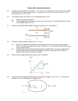
© Copyright 2026