Financial Analysis of 4G Network Deployment
Yanjiao Chen, Lingjie Duan, Qian Zhang
Abstract—Major cellular operators are planning to upgrade to
high-speed 4G networks, but due to budget constraints, they have
to dynamically plan and deploy the 4G networks through multiple
stages of time. By considering one-time deployment cost, daily
operational cost and 3G network congestion, this paper studies
how an operator financially manages the cash flow and plans the
4G deployment in a finite time horizon to maximize his final-stage
profit. The operator provides both the traditional 3G service and
the new 4G service, and we show that users will start to use the
4G service only when it reaches a sizable coverage. At each time
stage, the operator first decides an additional 4G deployment
size, by predicting users’ responses in choosing between the
3G and 4G services. We formulate this problem as a dynamic
programming problem, and propose an optimal threshold-based
4G deployment policy. We show that the operator will not deploy
to a full 4G coverage in an area with low user density or high
deployment/operational cost. Perhaps surprisingly, during the 4G
deployment process, we show that the 4G subscriber number first
increases and then decreases, as the 4G service helps mitigate 3G
network congestion and increases its QoS.
I. I NTRODUCTION
As the market penetration of smartphones increases and
more wireless users get used to data services, the existing 3G
networks become more and more congested. As the successor
of 3G, a 4G technology (e.g., LTE, featuring OFDM and
MIMO schemes) better utilizes the wireless resources, and
provides a much higher date rate to enable latest mobile
applications and resolve the network congestion [1]. Besides
this technological improvement, 4G service with a higher
data rate is more profitable than 3G in the wireless market.
According to [2], 4G service is usually priced significantly
higher than 3G even when 4G users keep similar data usage.
Hence, major cellular operators are planning to deploy the
new 4G service. However, they have to carefully plan their
4G deployment roadmap due to budget constraints. If not
well planned beforehand, they may experience an unexpected
financial cut-off. For example, as the 4G pioneer from 2008,
Sprint is now short of money to expand its 4G coverage and
has to request financial help from Softbank in Japan [3]. In
Europe, many operators are also budget-limited and are still
discussing when to deploy 4G [4].
The deployment of 4G network is not an overnight establishment but a long-term process requiring careful cash-flow
This work was supported by grants from 973 project 2013CB329006,
China NSFC under Grant 61173156, RGC under the contracts CERG
622613, 16212714, HKUST6/CRF/12R, and M-HKUST609/13, the grant
from Huawei-HKUST joint lab, the Competitive Earmarked Research Grants,
and the SUTD-MIT International Design Centre (IDC) Grant (Project No.:
IDSF1200106OH).
Y. Chen and Q. Zhang are with the Department of Computer Science and
Engineering, Hong Kong University of Science and Technology, {chenyanjiao,
qianzh}@ust.hk.
L. Duan is with the Engineering Systems and Design Pillar, Singapore
University of Technology and Design, lingjie [email protected].
management. An operator’s budget at a time is determined by
the operator’s initial funding, ongoing revenue collection, and
total cost till now. Revenue collected in the current stage, from
both 3G and 4G services, helps relax the budget constraint for
the next-stage deployment. The collected revenue is affected
by two major factors in the wireless market:
• User density is the number of all potential users in a
unit area who can choose and pay for cellular services.
We observe that in rural areas with a low user density,
it may not be profitable to deploy advanced and costly
4G networks. For example, Verizon densely deployed 4G
networks in populous states like New York, but only
sparsely deployed 4G networks in underpopulated states
like Utah [5].
• Market response is about all potential users’ service
choices, and such a response depends on service qualities (including network coverage, data rate, and network
congestion) and service prices. Users with high QoS requirements prefer 4G service, while those price-sensitive
ones prefer 3G service.
Accompanied with revenue collection, total cost of the 4G
network includes the deployment cost to physically enlarge
the 4G coverage and the operational cost to maintain the 4G
network all the time. More specifically,
• Deployment cost is the one-time expenditure to purchase
and build 4G network infrastructure (e.g., 4G cell towers).
According to [6], the cost to deploy a 4G LTE tower
ranges from US $75, 000 to US $200, 000, depending
on the leasing site. The 4G coverage is approximately
proportional to the number of 4G towers.
• Operational cost is the daily expenditure related to management and maintenance of 4G network (e.g., energy
and manpower costs), which is approximately proportional to the network coverage according to [7].
To our best knowledge, this paper is the first work that
financially studies the dynamic deployment planning for a
large-scale wireless network, by taking various costs and
market response into account. We consider a finite and timeslotted horizon.1 At each time stage, the operator first decides
his investment amount to expand the 4G coverage based on
his current budget, and users observing the network update
then choose between the 3G and 4G services. By predicting
users’ dynamic responses to the services qualities, the operator
wants to optimize his 4G deployment planning over time and
maximize the final-stage profit.
Our main results and key contributions are summarized as
follows:
1 A finite time horizon is reasonable as 4G has its own advantageous cycle
and may be replaced by another (e.g., 5G) in the future.
Financial modeling of cash flow for 4G deployment.
Very few studies have studied financial management in
wireless industry, and they assume the deployment of 4G
is an overnight effort and solve the static deployment
problem without considering the cash flow (e.g., [8] [9]).
Our financial model investigates the cash flow driven by
an operator’s initial budget, ongoing revenue collection
(depending on users’ dynamic subscriptions), and the
total cost for 4G network.
• Dynamic programming formulation for deployment planning. Since the operator’s current investment decision
affects next-stage budget and revenue collection, we formulate the cash flow management problem as a dynamic
program. The operator wants to maximize his final-stage
budget (cash level) by trading off deployment progress
and budget saving over time.
• Optimal threshold-based policy for 4G deployment. By
solving the dynamic program, we show that it is optimal
for the operator to accumulate the collected revenue till
a threshold for initial deployment. After starting with a
sizable deployment, the operator will gradually enlarge
the 4G coverage conforming to the time-varying budget
constraint. We also show that the operator should not
deploy to a full coverage in an under-populated area, or
if the deployment/operational cost is high.
• Impact of 3G network congestion. We show that the
expansion of 4G coverage helps resolve the 3G network congestion. As the 4G coverage increases, the 4G
service’s subscriber number can first increase but then
decrease as fewer subscribers churn from the improved
3G service to the 4G service.
The rest of the paper is organized as follows. We briefly
review the related work in Section II, and present the system
model in details in Section III. We analyze the market response
in Section IV, which is useful for the operator to predict and
decide optimal deployment policy in Section V. We study the
impact of operational cost in Section VI and the impact of 3G
congestion effect in Section VII. We present the simulation
results in Section VIII, and finally summarize the work in
Section IX. Due to page limitation, we give all the proofs
in our online technical report [10].
1
•
II. R ELATED W ORK
People just started to study network deployment or upgrade
problems recently. In [11], the Internet service providers
choose between “Upgrade” and “Not-Upgrade”, and pay a
one-time fee for infrastructure upgrade. In [12], Internet
providers choose an investment level to minimize their longterm security risk in a one-shot static model. In [13], the user
adoption of a new technology and an incumbent technology
is studied without considering network deployment process or
any economic return. In [8], wireless operators’ 4G network
upgrade is assumed to be an overnight establishment, without
considering the time duration and cash flow for deployment.
[9] analyzes the financial impact of pico-cellular base station
deployment by focusing on a static model without considering
2
t
……
Phase I: Operator decides to
expand the current 4G
coverage Qt-1 to Qt during
this time stage t
……
T
Phase II: Market response
Users observe Qt-1, and choose
3G, 4G or alternative service
3G
4G
Operator
Cellular users
Fig. 1: System model.
the deployment time or any dynamics in user subscription.
Task scheduling with energy constraints in cloud computing
has been studied in [14]–[16], but their optimizations do not
consider the change in payoff due to network update.
All prior works focus on a simplified one-time (static)
network upgrade, and our focus is on how an operator should
dynamically manage the cash flow for the 4G network deployment. Furthermore, we comprehensively incorporate users’
dynamic responses and various costs in the financial analysis.
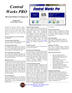
III. S YSTEM M ODEL
We consider a cellular operator, who plans to deploy a
new 4G network in a wireless market2 . We consider that the
operator has already deployed a ubiquitous 3G network, and
the area of this market region is normalized to 1. We denote
the user density as ρ in this region, and all ρ users are potential
subscribers to choose the 3G or 4G service provided by the
operator. The operator needs to make 4G deployment decisions
in a time-slotted horizon including a finite T stages, and the
decision-making in each stage t ∈ {1, ..., T } is further divided
into two phases as illustrated in Fig. 1:
•
•
Phase I (Operator planning): The 4G network coverage
at the beginning of time stage t is denoted as Qt−1 ,
depending on last time stage’s effort. Then the operator
will decide the enlarged 4G coverage by the end of time
stage t, Qt . Therefore, the 4G coverage expansion after
time stage t is Qt − Qt−1 ≥ 0.
Phase II (Market response): After Phase I, users will
choose their preferred service (or nothing), depending on
the current 4G coverage Qt−1 . Such a dependency on
Qt−1 rather than Qt is because that deploying a larger
Qt is still ongoing till the end of time stage t. After
deciding service choices for this time stage, users make
payments once and these payments can be used directly
for ongoing deployment in time stage t.
In the following, we will first introduce the models of 3G
and 4G services including their QoS requirements and prices,
and then specify users’ utility models in choosing different
services.
2 We plan to extend this monopoly model to oligopoly model in the
future, where the revenue collections among competitive operators are interdependent and operators have more incentive to deploy earlier as in [8].
3G service: The subscription fee of 3G service per time
stage is P 3G .3 Subscribers can access the mature 3G network
everywhere at a data rate R3G but may experience network
congestion.
4G service: The subscription fee of 4G service per time
stage is P 4G . Subscribers can connect to 4G network at a
high data rate R4G whenever they are within the 4G coverage
(Qt ≤ 1 after time stage t). According to the ITU standards,
3G and 4G data rates should be larger than 2 Mbit/s and 1
Gbit/s, respectively according to [18] [19], and the 4G service
price is globally 20% higher than 3G according to [2]. Thus
we reasonably assume that the quasi-unit-price of 4G is lower
than that of 3G (P 4G /R4G < P 3G /R3G ) 4 .
A user’s utility depends on his valuation of the service
choice and the price he pays. We adopt the widely-used multiattribute linear-weighted utility function (e.g., [20], [21]), and
define a subscriber’s utility as the difference between his
valuation of the chosen service and the service price. Since
different users have different sensitivity levels towards the QoS
in the valuation, we denote user-specific sensitivity level as α.
We follow a widely-used assumption that α follows uniform
distribution in a normalized range [0,1]. In Phase II of time
stage t + 1, given the 4G coverage Qt , a user with sensitivity
α has valuations αR3G and αR4G when choosing the two
services, and his utility when choosing 3G, 4G or none is:
 3G
if 3G
 uα (Qt ) = αR3G − P 3G ,
4G
3G
4G
u4G
(Q
)
=
α[Q
R
+
(1
−
Q
)R
]
−
P
,
if 4G
t
t
t
 α
u0 .
o.w.
(1)
where Qt R4G + (1 − Qt )R3G is the 4G service’s expected
data rate by considering the actual rate R4G in 4G coverage
Qt and rate R3G in uncovered area 1−Qt . For ease of analysis,
the congestion effect in the 3G network is not presented here
and will be modeled later in Section VII for clear comparison
purpose.
As shown in Fig. 1, in each time stage, the operator in Phase
I needs to decide deployment after predicting users’ responses
in Phase II for revenue collection, and users’ responses are
determined by their utilities. By using backward induction, we
will first analyze the market response in phase II in different
time stages in Section IV, then analyze the operator’s optimal
4G deployment in phase I in different time stages in Section
V.
IV. M ARKET R ESPONSE A NALYSIS FOR R EVENUE
E STIMATION
In this section, we analyze the market response in Phase II
of time stage t + 1, t ∈ [0, T ] given the 4G coverage Qt . The
choice of a user with QoS sensitivity α is:
3 The subscription fee can be monthly based. We assume a flat-rate fee
model here, which is a common practice in the existing data market [17].
4 We consider arbitrary price values and assume that the 3G and 4G prices
are static. This is reasonable as the time scale of each stage is about one
month, but the price is not flexible to change from time to time as users in
practice do not welcome price change.

4G
if u3G
 3G service,
α (t) ≥ max{uα (Qt ), u0 },
4G
4G service,
if uα (Qt ) ≥ max{u3G
α (Qt ), u0 },

No subscription, otherwise.
For ease of reading, we denote the price difference and QoS
difference as ∆P = P 4G − P 3G , and ∆R = R4G − R3G .
By comparing all users’ utilities of different choices, we can
partition users’ choices according to three α thresholds:
3G
• α(3,0) = P
/R3G partitions users in choosing between
3G service and no subscription. A user with α ≥ α(3,0)
prefers 3G service to no subscription.
4G
• α(4,0) = P
/(QR4G + (1 − Q)R3G ) partitions users in
choosing between 4G service and no subscription. A user
with α ≥ α(4,0) prefers 4G service to no subscription.
• α(4,3) = ∆P /(Q∆R) partitions users in choosing between 3G and 4G services. A user with α ≥ α(4,3) prefers
4G service to 3G service.
Note that α(4,0) and α(4,3) increase with Qt , since the expansion of 4G network will attract more subscribers to 4G
service.
Based on the above analysis, we can derive the users’
equilibrium subscription in Phase II and estimate the resultant
revenue R(Qt ) for the operator in Phase I of each time stage.
The operator’s revenue R(Qt ) depends on Qt and is the sum
of subscription fee collected from both services.
Proposition 1. Depending on the 4G coverage Qt , the operator’s revenue in time stage t + 1 is:
• Low 4G coverage regime. When Qt < ∆P /∆R, no users
choose 4G service and users with α ∈ [α(3,0) , 1] choose
3G. The operator’s current revenue is:
R(Qt ) = ρP 3G (1 − P 3G /R3G ).
(2)
•
Medium 4G coverage regime. When ∆P /∆R ≤ Qt <
∆P R3G /(P 3G ∆R), users with α ∈ [α(3,0) , α(4,3) ]
choose 3G, and α ∈ [α(4,3) , 1] choose 4G. The operator’s
current revenue is:
(P 3G )2
∆P 2
4G
−
.
(3)
R(Qt ) = ρ P −
Qt ∆R
R3G
•
High 4G coverage regime. When Qt
≥
∆P R3G /(P 3G ∆R),5 no users choose 3G service
and users with α ∈ [α(4,0) , 1] choose 4G. The operator’s
current revenue is:
P 4G
R(Qt ) = P 4G 1 −
.
(4)
Qt ∆R + R3G
In low 4G coverage regime, compared with the existing
3G service, 4G service is not attractive to any user, and one
can imagine that the operator should initially deploy beyond
this regime directly, if budget allows. It should be noted that
as Qt increases, the operator’s revenue in both medium and
high coverage regimes will increase. The revenue increase in
5 Due to the fact P 3G /R3G > P 4G /R4G in Section III, we can prove
∆P R3G /(P 3G ∆R) < 1 and the high coverage regime exists.
the high coverage regime is faster, as 4G further attracts the
original users out of 3G service and the operator’s market
penetration increases.
V. DYNAMIC P ROGRAMMING F ORMULATION FOR
O PTIMAL 4G D EPLOYMENT
In this section, we formulate the operator’s deployment
problem as a dynamic program to maximize the final-stage
cash level and analytically solve the optimization problem.
We want to first characterize the deployment policy with
the deployment cost only, which serves as a benchmark to
compare with the additions of operational cost in Section VI
and congestion effect in Section VII6 .
Let St denote the operator’s cash level at the end of time
stage t. St depends on three parts: 1) St−1 , the cash level at
the end of time stage t − 1, 2) R(Qt−1 ) given in Proposition
1, operator’s revenue collected during time stage t based on
Qt−1 , and 3) the deployment cost from Qt−1 to Qt . S0 is
the initial budget before time stage t = 1. The state transition
function of cash flow is:
(5)
in which f (Qt , Qt−1 ) is the deployment cost function during
time stage t. We need to make sure that the budget constraint
holds under current deployment investment, that is, St should
be non-negative for any time stage t. We do not allow capital
raise to fill in the cash flow gap.
To manage the cash flow, the operator makes decisions from
time stages 1 to T , that is, to decide Q1 , ..., QT . The objective
is to maximize the final profit (cash level), denoted as ST +1 ,
which consists of 1) ST , the cash level at the end of time
stage T , and 2) R(QT ), operator’s revenue based on market
response to QT . The operator will not further deploy 4G in
stage T . That is,
ST +1 = ST + R(QT ).
(6)
By deciding deployment plan Qt for each stage, the operator
wants to maximize ST +1 , subject to the budget constraint
and cash level transition equation. The dynamic programming
problem is:
max
Q1 ,...,QT
s.t.
ST +1
St ≥ 0, ∀t = 1, · · · , T,
St = St−1 + R(Qt−1 ) − f (Qt , Qt−1 ),
0 ≤ Q1 ≤ Q2 ≤ · · · ≤ QT ≤ 1.
max
S0
|{z}
Q1 ,··· ,QT
initial budget
(7)
The deployment cost of enlarging the 4G coverage is mainly
the cost to purchase and set up 4G base stations, and this cost
can be approximated as a linear function of the number of 4G
base stations according to [9]. In our online technical report
6 We assume that the 4G spectrum license has already been obtained before
the deployment, so we do not consider spectrum cost in this paper.
+
T
X
R(Qt ) −
t=0
|
{z
}
C Q
| d{z T}
total deployment cost
revenue f low
s.t. S0 +
A. Dynamic Programming Formulation
St = St−1 + R(Qt−1 ) − f (Qt , Qt−1 ), t ∈ {1, ..., T },
[10], we also investigate Verizon’s real data to show this linear
relationship. Thus, we reasonably assume that the deployment
cost function is f (Qt+1 , Qt ) = Cd (Qt+1 − Qt ), in which Cd
is the unit deployment cost to purchase and install 4G base
stations per unit coverage. By substituting the state transition
function of the cash flow in (5) and the final-stage cash level
in (6) into the objective of problem (7), we can simplify the
problem as:
t−1
X
R(Qτ ) − Cd Qt ≥ 0, t = 2, ..., T
τ =1
S0 − Cd Q1 ≥ 0,
0 ≤ Q1 ≤ ... ≤ QT ≤ 1.
(8)
where the first constraint is the budget constraint to ensure
that the cash level at each time stage is non-negative.
B. Optimal deployment policy
The dynamic programming problem in (8) is difficult to
solve. This is because R(Qt ) in the objective and budget
constraints is not concave, and the optimization problem is
not convex.
Lemma 1. R(Qt ) is concave within two separate Qt ranges
[0, ∆P /∆R] and (∆P /∆R, 1], respectively7 , but is just quasiconcave (not concave) in the entire range Qt ∈ [0, 1].
To make the problem (8) solvable, we decompose the
problem into two convex subproblems by focusing on the Qt
ranges [0, ∆P /∆R] and (∆P /∆R, 1], respectively. First, we
define Tth ∈ {1, ..., T } as the threshold time stage, such that
Qt ≤ ∆P /∆R, ∀t ≤ Tth − 1, and Qt > ∆P /∆R, ∀t ≥ Tth .
Due to the budget constraint in (8), the feasible regime of Tth
is:
Tth ≥ (Cd ∆P/∆R − S0 )/(ρP 3G (1 − P 3G /R3G )) . (9)
Then, we solve the optimization problem by the following
three steps:
1) Optimal deployment policy before time stage Tth . Given
any Tth value, we find the optimal 4G deployment policy
for the convex optimization problem (8) by optimizing
over Q1 to QTth −1 and replacing the last constraint with
Q1 ≤ · · · ≤ QTth −1 ≤ ∆P/∆R.
2) Optimal deployment policy after time stage Tth . Given
any Tth value, we find the optimal 4G deployment policy
for the convex optimization problem by optimizing over
QTth to QT and replacing the last constraint with
∆P/∆R ≤ QTth ≤ · · · ≤ QT .
∗
3) Search of the optimal Tth
. By changing Tth and comparing all ST +1 values given by the two subproblems,
7 Recall
that ∆P/∆R < 1 as we assume P 3G /R3G > P 4G /R4G .
∗
we can find the optimal Tth
yielding the largest value
∗
ST +1 .
By following the first step before time stage Tth , we have
the following result.
Proposition 2. (Optimal deployment policy before time stage
Tth ) It is the best for the operator not to deploy any 4G
network before Tth . That is, Q∗t = 0, 1 ≤ t ≤ Tth − 1.
Algorithm 1 Calculation of mature deployment stage T¯th
Set t = Tth − 1, Qm
t = ∆P/∆R.
if Cd > (T + Tth − t)R0 (Qm
t ) then
3:
Set T¯th = Tth − 1; STOP;
4: else
5:
Set Q∗t = Qm
t , t=t+1
1:
2:
6:
Qm
t = min{1, (S0 +
Based on Proposition 2, we can rewrite the optimization
problem (8) as
QTth ,··· ,QT
T
X
P 3G
Tth ρP 3G (1 − 3G ) +
R(Qt ) − Cd QT
{z R } t=Tth
|
t−1
X
P 3G
)
+
R(Qτ ) − Cd Qt ≥ 0,
R3G
τ =Tth
∀t = Tth , ..., T
∆P/∆R ≤ QTth ≤ ... ≤ QT ≤ 1
(11)
if
Cd > max{(T + Tth − t)R0 (Q∗t−1 ), (T + Tth −
t)R0 (Qm
t )}, or;
2)
Cd ∈ [(T +Tth −t)R0 (Q∗t−1 ), (T +Tth −t)R0 (Qm
t )],
or;
3)
Cd < min{(T + Tth − t)R0 (Q∗t−1 ), (T + Tth −
m
t)R0 (Qm
t )}, but Qt = 1 or t = T .
then
Set T¯th = t; STOP;
else
GOTO step 5.
end if
end if
1)
revenue bef ore Tth
s.t. S0 + Tth ρP 3G (1 −
R(Q∗τ ))/Cd }
τ =0
7:
max
t−1
X
(10) 8:
Since the objective function and the constraints in (10) are
convex, KKT conditions, the first order necessary conditions,
are also sufficient for a solution to be optimal [22]. We show
that the optimal idea is to find the “stopping time stage” T¯th ≥
Tth − 1, such that before the time stage T¯th , the operator will
use all current budget to deploy 4G in each time stage (with
tight budget constraint in (8)); after the time stage T¯th , no more
new 4G network is deployed. The only problem is how to find
the final 4G coverage at time stage T¯th , which depends on
the deployment cost Cd , time length T , and revenue function
R(Qt ). Let Q∗t denote the optimal 4G coverage at time stage
t with Tth ≤ t ≤ T . By solving the subproblem we have the
following proposition.
Proposition 3. (Optimal deployment policy after time stage
Tth ) Given any Tth value, there exists a mature deployment
stage T¯th , before and after which the operator has different
deployment strategies. The value of T¯th is determined by
Algorithm 1. The special case of T¯th =Tth − 1 leads to no
further deployment after Tth , i.e., Q∗t = QTth −1 for any time
stages t ∈ {Tth , ..., T }. More generally, when T¯th > Tth − 1,
we have:
• Aggressive deployment period: In the time stages t ∈
[Tth , T¯th ], the operator will use up all his current budget
at each time stage t for 4G deployment, i.e., Q∗t = Qm
t
in (11), the maximum achievable coverage that can be
supported by the budget at time stage t.
¯th , the
• Conservative deployment period: When t = T
operator will conservatively upgrade according to:
 ∗
0
(Q∗t−1 ), R0 (Qm

t )}
 Q∗t−1 , if Cd > (T + Tth − t) max{R

0
∗
qt ,
if Cd ∈ [(T + Tth − t)R (Qt−1 ),
(T + Tth − t)R0 (Qm

t )]

 m
Qt ,
if Cd < (T + Tth − t) min{R0 (Q∗t−1 ), R0 (Qm
t )}
in which qt∗ is the unique solution to the equation Cd =
(T + Tth − t)R0 (qt∗ ).
9:
10:
11:
12:
•
No deployment period. When T¯th + 1 ≤ t ≤ T , Q∗t =
Q∗t−1 .
Intuitively, the final optimal 4G coverage requires that the
marginal cost Cd equals the marginal revenue (T + Tth −
t)R0 (qt∗ ). If T¯th = Tth , aggressive deployment period does
not exist. If T¯th = T , conservative coverage period does not
exist.
After solving the two subproblems in Propositions 2 and 3,
now we are ready to combine their solutions for the global
optimum, by searching through all possible Tth values.
Lemma 2. The optimal Tth is chosen from the following two
candidates:
• Tth = T + 1, that is, the operator will not deploy 4G
network to a coverage level ∆P/∆R;
• Tth =
(Cd ∆P/∆R − S0 )/[ρP 3G (1 − P 3G /R3G )] ,
that is, the operator deploys the 4G network to the
coverage level ∆P/∆R as soon as possible.
Lemma 2 helps us limit our attention to two candidates only,
without widely searching all Tth values. Finally, to determine
which Tth candidate is better, we compare their corresponding
final-stage cash levels ST +1 : the one that yields a higher final∗
stage cash level is the optimal Tth
.
By following the above decompose-and-compare approach,
we summarize the optimal 4G deployment policy.
Theorem 1. The optimal 4G deployment policy is one of the
following two options.
• No deployment scheme: the operator never deploys any
4G network, i.e., Q∗t = 0, t = 1, ..., T .
∗
Threshold-based
deployment scheme: Set threshold
Tth
=
3G
3G
3G
(Cd ∆P/∆R − S0 )/[ρP (1 − P /R )] .
∗
– When t ∈ [1, Tth
− 1], the operator does not deploy
any 4G network, i.e., Q∗t = 0;
∗
– When t ∈ [Tth
, T ], the operator deploys 4G network
according to Proposition 3.
The special case is that, if the deployment cost satisfies
Cd ∆P/∆R − S0
ρ∆R, (12)
Cd > T + 1 −
ρP 3G (1 − P 3G /R3G )
•
the No deployment scheme is optimal.
Notice that the right-hand side term in (12) is increasing
in user density ρ, therefore (12) is more likely to hold as
ρ decreases. This tells us that when user density is low, the
operator is unwilling to deploy 4G network. Moreover, if the
time length T is long enough, any one-time deployment cost
Cd is negligible compared to the infinitely long 4G benefit,
and initial 4G deployment will be started as soon as possible.
Proposition 4. Final 4G coverage level Q∗T increases with
time length T and user density ρ, but decreases with the
deployment cost Cd . As T → ∞, Q∗T = 1 (full 4G coverage).
As T increases, the operator has more time to collect the
4G revenue. As ρ increases, a higher revenue can be collected
from more users, encouraging the operator to increase the 4G
coverage. Finally, if Cd is large, the operator wants to avoid
high deployment cost by deploying a smaller 4G coverage.
In this section, we model and analyze how the operational
cost affects the operator’s 4G deployment policy, by comparing
with Section V under deployment cost only. The operational
cost (OPEX) is related to daily management and maintenance
of 4G network, which can be approximated as a linear function
of the network coverage with unit cost Co according to [7]
[23]. In time stage t + 1, the total deployment and operational
cost is
f (Qt+1 , Qt ) = Cd (Qt+1 − Qt ) + Co Qt .
(13)
By adding the operational cost Co Qt in each time t, the
optimization problem in (8) becomes
Q1 ,··· ,QT
T
X
R(Qt ) − Cd QT −
Co
t=1
T
X
Qt
t=1
|
{z
}
total operational cost
s.t. S0 +
t−1
X
if Cd > (T + Tth − t) max{(R0 (Q∗t−1 ) − Co ),
(R0 (Qm
t ) − Co )}
if Cd ∈ [(T + Tth − t)(R0 (Q∗t−1 ) − Co ),
(T + Tth − t)(R0 (Qm
t ) − Co )]
if Cd < (T + Tth − t) min{(R0 (Q∗t−1 ) − Co ),
(R0 (Qm
t ) − Co )}
(15)
in which qt∗ is the unique solution to the equation Cd = (T +
Tth − t)(R0 (qt∗ ) − Co ).
Based on these results, we can search for the optimal Tth .
Recall that in Lemma 2, if there is no operational cost, one of
the two possible choices of Tth suggests the operator deploy
the 4G coverage above ∆P/∆R once collecting enough
budget. However, with operational cost, this choice may not
be optimal as the marginal revenue at coverage ∆P/∆R may
be less than the marginal revenue at the initial coverage level
0.
∗
Lemma 3. The optimal Tth
with consideration of the operational cost, is chosen from the following two candidates:
•
τ =1
(14)
By following a similar 3-step solution approach as in Section
V with a threshold stage Tth , we can first propose the optimal
deployment policy before time stage Tth and the optimal
R(QTe) − Co QTe ≥ R(0)
(16)
R(QTe−1 ) − Co QTe−1 ≤ R(0)
(17)
Theorem 2. (Optimal 4G deployment policy with operational
cost). The optimal 4G deployment policy is one of the following two options.
•
S0 − Cd Q1 ≥ 0,
Tth = T + 1, that is, the operator will not deploy the 4G
coverage to ∆P/∆R;
Tth = Te, which satisfies
Lemma 3 shows that it is the best for the operator to
wait until he can immediately reach a sizable and profitable
coverage level satisfying (16) and (17), where the marginal
revenue (depending on the coverage level) is larger than the
marginal revenue R(0) without 4G deployment.
According to the discussion above, by using the decomposeand-compare approach, we have the following theorem for the
optimal 4G deployment policy with operational cost.
•
(R(Qτ ) − Co Qτ ) − Cd Qt ≥ 0, t = 2, ..., T
0 ≤ Q1 ≤ ... ≤ QT ≤ 1
 ∗
Qt−1 ,






 ∗
qt ,




,
 Qm

 t
•
VI. I MPACT OF O PERATIONAL C OST
max S0 +
deployment policy after Tth , and finally compare and find the
∗
optimal Tth
.
Due to page limit, we skip the detailed analysis here. The
Optimal deployment policy before time stage Tth is the same
as Proposition 2 in Section V. And the Optimal deployment
policy after time stage Tth is similar to Proposition 3, by
changing (3) to:
No deployment scheme: the operator never deploys any
4G network, i.e., Q∗t = 0, t = 1, ..., T .
Threshold-based deployment scheme:
∗
– When t ∈ [1, Tth
− 1], the operator does not deploy
any 4G network, i.e., Q∗t = 0;
∗
– When t ∈ [Tth
, T ], the operator deploys 4G network
according to Proposition 3 by replacing (3) with (15);
∗
– Tth
is determined by Lemma 3.
By comparing the final-stage cash levels of the above two
options, the one that yields higher final-stage cash level is the
optimal choice. The operational cost changes the optimal 4G
deployment in two aspects.
Proposition 5. The operational cost reduces the final 4G
coverage level, and delays the time to deploy the 4G network.
Without operational cost, Proposition 4 tells that Q∗T = 1
as T → ∞. However, when there exists an operational cost,
and the cost is high enough (R0 (Qt ) < Co ), we can show
that no matter how large T is, the operator will never deploy
4G network. If the operational cost is not that high, to
compensate for the operational cost, the operator will first
accumulate enough budget during a longer time for a sizable
initial deployment coverage.
VII. I MPACT OF N ETWORK C ONGESTION
In this section, we model and analyze the congestion
effect in the 3G network by comparing to the congestion-free
scenario in Section V.8 Note that the network congestion in 4G
network is incomparable compared to 3G network. Actually,
4G technology is proposed to resolve the network congestion.
The congestion affects the QoS and users’ responses in
Phase II, which should be taken into account into the operator’s deployment planning in Phase I in each time stage. More
specifically, the revenue function R(Qt ) in time stage t under
congestion effect is now different from that in Proposition 1.
Both optimal 4G deployment policies in Theorem 1 and 2 can
be applied by replacing congestion-free revenue function with
revenue function with congestion effect. Due to page limit, in
the following, we only look at the modeling and calculation
of the revenue function R(·).
As 3G users’ traffic increases, the network congestion
increases and reduces the 3G QoS. Let g(·) denote the 3G
congestion cost, which is an increasing function of the number
of the users in 3G network. Note that these users include
not only 3G subscribers but also 4G subscribers roaming
outside 4G coverage. Let Dt denote the number of total users
connecting to 3G network. By incorporating the congestion
effect, given the 4G coverage Qt , users’ utility function
changes from (1) to:
3G
u3G
− g(Dt ) − P 3G
α (Qt ) = αR
(18)
4G
u4G
+ (1 − Qt )[αR3G − g(Dt )] − P 4G (19)
α (Qt ) = αQt R
We assume that g(·) is linear in user demand, i.e., g(x) =
γx, which is a common approximation (e.g., [21]) to make the
problem tractable and deliver clean engineering insight. When
γ = 0, the results will degenerate to be the same as those
in Section IV. Similar to Section IV, we can partition user’s
choices according to three thresholds:
3G
• α(3,0) = (P
+ γDt )/R3G partitions users in choosing
between 3G service and no subscription. A user with α >
α(3,0) prefers 3G service to no subscription.
8 Note that we do not directly compare to Section VI as the comparison is
not clean to tell the impact of congestion effect.
α(4,0) = (P 4G + (1 − Qt )γDt )/(Qt ∆R + R3G ) partitions users in choosing between 4G service and no
subscription. A user with α > α(4,0) prefers 4G service
to no subscription.
• α(4,3) = (∆P − Qt γDt )/(Qt ∆R) partitions users in
choosing between 3G and 4G services. A user with
α > α(4,3) prefers the 4G service to 3G service.
When there is no congestion effect in Section IV, the three
thresholds are independent of the equilibrium number of users
who choose 3G and 4G service, i.e., Dt . However, when there
is congestion effect, the three thresholds are functions of Dt ,
making it difficult to obtain the equilibrium market response.
Despite complexity, we present the operator’s revenue under
congestion effect in Proposition 6, which is quite different
from Proposition 1.
•
Proposition 6. Depending on the 4G coverage Qt , the operator’s revenue is:
• Low 4G coverage regime. No users choose 4G service
and users with α ∈ [α(3,0) , 1] choose 3G. The operator’s
revenue is:
R(Qt ) = P 3G
•
R3G − P 3G
.
R3G + γ
Medium 4G coverage regime. Users with α ∈
[α(3,0) , α(4,3) ] choose 3G, and α ∈ [α(4,3) , 1] choose 4G.
The operator’s revenue is:
R(Qt ) =
P
3G
∆P R3G
Qt
− ∆RP 3G + γ(1 − Qt )(P 3G − R4G +
∆RR3G
∆P
Qt
)
γ(R3G Qt
+
+ ∆R)
3G
3G
4G
∆RR
−
∆P
R
/Q
+
γ(R
− P 3G − ∆P/Qt )
t
+ P 4G
∆RR3G + γ(R3G Qt + ∆R)
•
High 4G coverage regime. No users choose 3G service
and users with α ∈ [α(4,0) , 1] choose 4G. The operator’s
revenue is:
R(Qt ) = P 4G
Qt ∆R + R3G − P 4G
Qt ∆R + R3G + (1 − Qt )2 γ
The cutting point between the Low and Medium 4G coverage regime is lower when 3G congestion is considered,
because the 3G congestion encourages users to switch to 4G
service even when 4G coverage is small. We can see that
R(Qt ) is greatly influenced by the congestion factor γ. We
will analyze by numerical results the influence of congestion
effect on 4G deployment in Section VIII.
VIII. N UMERICAL R ESULTS
In this section, we use numerical results to illustrate and
highlight some interesting engineering insights.
A. Impact of User Density, Service Prices, and Time Span
1) The user density: Fig. 2(a) shows that a higher user
density ρ boosts the 4G deployment because there are more
potential subscribers and the total 4G revenue is higher. When
the user density is below a certain threshold, it is optimal for
1
ρ=2
ρ = 2.5
ρ = 3.5
0.8
0.6
0.4
0.2
0
0
5
10
15
1
0.8
0.6
0.4
T = 10
T = 20
T = 30
0.2
0
0
20
5
10
Time horizon
15
20
25
Optimal 4G coverage level
Optimal 4G coverage level
Optimal 4G coverage level
1
0.8
0.6
0.4
0
0
30
Cd = 15
Cd = 20
Cd = 25
0.2
5
Time horizon
(a) Impact of user density ρ
10
15
20
Time horizon
(b) Impact of T
(c) Impact of Cd
Fig. 2: Impact of the user density, time span and deployment cost.
0.65
0.8
3G subscriber, no congestion
4G subscriber, no congestion
3G subscriber, congestion
4G subscriber, congestion
0.5
0.4
0.3
0.2
0.1
0
0
0.2
0.4
0.6
0.8
4G Coverage
(a) 3G and 4G subscriber numbers
0.45
0.55
0.4
0.5
0.35
Revenue
0.6
0.5
No congestion
Congestoin
0.6
Total subscribers
Subscriber ratio
0.7
0.45
0.4
0.3
0.25
0.35
0.2
0.3
0.15
0.25
0
0.2
0.4
0.6
0.8
4G Coverage
(b) Total subscriber numbers
No congestion
Congestion
0.1
0
0.2
0.4
0.6
0.8
4G Coverage
(c) Total revenue at a time stage
Fig. 3: Impact of the 3G congestion effect on the revenue and market response.
the operator not to deploy 4G network (See the ρ = 2 case).
This explains why in some under-populated rural area, there
is no 4G development.
2) Time span: Fig. 2(b) shows that the time span T does not
change the optimal 4G deployment progress in the aggressive
deployment stage (Tth ≤ t ≤ T¯th ), but it does change the final
4G coverage level Q∗T . Shorter T decreases T¯th in Lemma 2 of
Section V, the time stage when there is no more deployment.
Larger T increases the final 4G coverage. Intuitively, as the
time span T decreases, the operator has fewer time stages
to collect the revenue from the newly deployed 4G network.
Therefore, the operator stops at an earlier time stage for
deployment and saves the deployment cost. We can also
observe from Fig. 2(c) that, if T is long enough, the operator
deploys a full coverage 4G network as the long-term 4G
benefits outweigh the one-time deployment cost.
B. Impact of Deployment and Operational Costs
1) Deployment cost: Fig. 2(c) shows the 4G deployment
roadmap as a function of time and deployment cost Cd . A
larger deployment cost will reduce the final 4G deployment
coverage, and delay the initial time stage when the operator
starts to deploy. Actually, it can be proved theoretically that
QT decreases with Cd (see [10]). The operator starts to deploy
4G network later because he needs more time to collect enough
budget to reach sizable coverage ∆P/∆R.
2) Operational Cost: Fig. 4(a) shows that a larger operational cost delays the deployment timing and reduces the
final 4G coverage level. The difference between operational
cost and deployment cost is that, there is no deployment cost
once the 4G coverage becomes stable, but the operational cost
always exists. If the time horizon T is large enough, with
only deployment cost, the 4G network will always reach full
coverage. However, with operational cost, if the difference
between the marginal revenue R0 (Q∗T = 1) is smaller than
the operational cost Co , the 4G network will never reach full
coverage no matter how large T is, according to Theorem 2.
This is illustrated in the case of Co = 3 in Fig. 4(a).
C. Impact of Congestion Effect
Fig. 3 shows the impact of the congestion effect with
coefficient γ on the market response and revenue, depending
on different 4G coverage levels. Fig. 3(a) shows that, when
the 4G coverage is small but still attractive to users (between
0.2 and 0.5), there are more 4G subscribers when there is 3G
congestion, but when the 4G coverage is large (more than 0.5),
there are fewer 4G subscribers. This is because, the increase
in 4G coverage initially eases the 3G congestion, but later
aggravates the 3G congestion since more 4G subscribers connect to 3G network. Fig. 3(b)(c) further show that congestion
effect reduces the total subscriber number and the operator’s
revenue.
Figs. 4(b)(c) show that the congestion effect delays the
deployment timing, because the revenue collected over time
is smaller and the operator needs more time to collect enough
budget to reach the initial coverage threshold ∆P/∆R. If the
operational cost Co is low, the final 4G coverage decreases as
the congestion factor γ increases, as shown in Fig. 4(b). But if
the operational cost Co is high, the final 4G coverage increases
with γ, as shown in Fig. 4(c). One possible explanation for
Optimal 4G coverage level
Optimal 4G coverage level
0.8
0.6
0.4
Co = 0
Co = 1
Co = 1.5
Co = 2
0.2
0
0
5
10
15
20
0.8
Optimal 4G coverage level
1
1
0.8
0.6
0.4
γ=0
γ=1
γ=2
0.2
0
0
5
10
15
20
0.7
0.6
0.5
0.4
0.3
0.1
0
0
Time horizon
Time horizon
(a) Impact of Co
γ=0
γ=1
γ=2
0.2
(b) Impact of γ, Co = 0.1
5
10
15
20
Time horizon
(c) Impact of γ, Co = 1
Fig. 4: Impact of operational cost and congestion effect.
these two different directions of final 4G coverage versus
congestion factor γ is as follows. When the operational cost
is high (Fig.4(c)), the final 4G coverage is relatively low
(around 0.7), thus the 4G subscribers are relatively low. The
3G congestion mostly results from 3G subscribers. So the
increase in γ encourages the operator to deploy more 4G
coverage to ease 3G congestion effect. When the operational
cost is low (Fig.4(b)), the final 4G coverage is relatively high
(around 0.9), thus the 4G subscribers are relatively high. The
3G congestion mostly results from 4G subscribers who access
3G network. So the operator instead decreases 4G coverage
when 3G congestion factor γ increases.
IX. C ONCLUSION
In this paper, we conduct financial analysis for 4G network
deployment. We model the operator’s cash flow management
as a dynamic process through a limited time horizon: at each
time stage, the operator decides the 4G deployment level
with the budget constraint. The goal is to maximize the final
cash level, which can be formulated as an optimization problem, and we solve the problem using dynamic programming.
A practical and easy-to-implement optimal 4G deployment
policy is proposed. In the first phase, the operator always
exhausts the capital for deployment. In the second phase,
the operator strategically sets the coverage level, which will
remain unchanged in the third phase. We find that the operator
delays the 4G deployment timing and reduces the final 4G
coverage level if there is operational cost because the marginal
revenue becomes smaller. We further consider the congestion
effect in the 3G network and show that it results in a lower
total subscription level, a lower revenue, and a smaller final
4G coverage.
There are several future directions. First, we may consider
the discounted cash flow, and the reduction in deployment
and operational costs due to technology advancement. Second,
we may also consider uncertainties in user response, as some
users may not be rational enough to make optimal decisions.
Finally, we may consider the bandwidth reallocation between
the growing 4G service and traditional 3G service.
R EFERENCES
[1] “4g LTE market upgrade,” Actiontec Corporation, White paper, 2010.
[2] ABIresearch, “4G data is priced 20 percent higher than
3G,” 2012. [Online]. Available: https://www.abiresearch.com/press/
4g-data-is-priced-20-higher-than-3g
[3] “Sprint still bleeding customers, money; looks to softbank to finance
LTE upgrade,” 2013. [Online]. Available: http://www.dailytech.com
[4] “Teliasonera layoffs a sign of trouble for mobile operators,” TECH
EUROPE, http://blogs.wsj.com/tech-europe, 2012.
[5] “4G LTE coverage.” [Online]. Available: http://www.verizonwireless.
com/wcms/consumer/4g-lte.html
[6] “How much do cell tower cost,” 2011. [Online]. Available: www.
deadzones.com
[7] “Construction, not capacity, is the real lte challenge in U.S.” 2012.
[Online]. Available: http://www.telecomengine.com
[8] L. Duan, J. Huang, and J. Walrand, “Economic analysis of 4G network
upgrade,” in IEEE, INFOCOM 2013.
[9] H. Claussen, L. T. Ho, and L. G. Samuel, “Financial analysis of a picocellular home network deployment,” in IEEE International Conference
on Communications (ICC), 2007, pp. 5604–5609.
[10] “Technical report of financial analysis of 4G network deployment,” https:
//www.dropbox.com/s/zx74gtphrm3chnb/TechnicalReport.pdf.
[11] J. Musacchio, J. Walrand, and S. Wu, “A game theoretic model for
network upgrade decisions,” in Proceedings of the 44th Annual Allerton
Conference on Communication, Control, and Computing, Monticello, IL,
2006, pp. 191–200.
[12] L. Jiang, V. Anantharam, and J. Walrand, “How bad are selfish investments in network security?” IEEE/ACM Transactions on Networking
(TON), vol. 19, no. 2, pp. 549–560, 2011.
[13] S. Sen, Y. Jin, R. Gu´erin, and K. Hosanagar, “Modeling the dynamics
of network technology adoption and the role of converters,” IEEE/ACM
Transactions on Networking (TON), vol. 18, no. 6, pp. 1793–1805, 2010.
[14] W. Zhang, Y. Wen, and D. O. Wu, “Energy-efficient scheduling policy for collaborative execution in mobile cloud computing,” in IEEE
INFOCOM, 2013, pp. 190–194.
[15] Y. Jin, Y. Wen, Q. Chen, and Z. Zhu, “An empirical investigation of
the impact of server virtualization on energy efficiency for green data
center,” The Computer Journal, vol. 56, no. 8, pp. 977–990, 2013.
[16] Y. Jin, Y. Wen, and Q. Chen, “Energy efficiency and server virtualization in data centers: An empirical investigation,” in IEEE INFOCOM
Computer Communications Workshops, 2012, pp. 133–138.
[17] R. W. Costas Courcoubetis, Pricing Communication Networks: Economics, Technology and Modelling. WILEY, 2003.
[18] ITU, “Cellular standards for the third generation,” 2005. [Online].
Available: http://www.itu.int/osg/spu/imt-2000/technology.html
[19] ——, “ITU global standard for international mobile telecommunications
’IMT-advanced’,” 2008. [Online]. Available: http://www.itu.int/ITU-R/
information/promotion/e-flash/2/article4.html
[20] R. L. Keeney, Decisions with multiple objectives: preferences and value
trade-offs. Cambridge University Press, 1993.
[21] C. Joe-Wong, S. Sen, and S. Ha, “Offering supplementary wireless
technologies: Adoption behavior and offloading benefits,” in IEEE,
INFOCOM 2013.
[22] S. P. Boyd and L. Vandenberghe, Convex optimization. Cambridge
university press, 2004.
[23] L. Duan, J. Huang, and B. Shou, “Economics of femtocell service
provision,” IEEE Transactions on Mobile Computing, vol. 12, no. 11,
pp. 2261–2273, 2013.