
Problems and Solutions for Ordinary Diffferential Equations
Problems and Solutions for Ordinary Diffferential Equations by Willi-Hans Steeb International School for Scientific Computing at University of Johannesburg, South Africa and by Yorick Hardy Department of Mathematical Sciences at University of South Africa, South Africa updated: June 16, 2015 Preface The purpose of this book is to supply a collection of problems for ordinary differential equations. Prescribed books for problems. 1) Continous Symmetries, Lie Algebras, Differential Equations and Computer Algebra, second edition by Willi-Hans Steeb World Scientific Publishing, Singapore 2007 ISBN 981-256-916-2 http://www.worldscibooks.com/physics/6515.html 2) Problems and Solutions in Theoretical and Mathematical Physics, third edition, Volume I: Introductory Level by Willi-Hans Steeb World Scientific, Singapore, 2009 ISBN-13 978-981-4282-14-7 http://www.worldscibooks.com/physics/7416.html 3) Problems and Solutions in Theoretical and Mathematical Physics, third edition, Volume II: Advanced Level by Willi-Hans Steeb World Scientific, Singapore, 2009 ISBN-13 978-981-4282-16-1 http://www.worldscibooks.com/physics/7416.html v The International School for Scientific Computing (ISSC) provides certificate courses for this subject. Please contact the author if you want to do this course or other courses of the ISSC. e-mail addresses of the author: [email protected] [email protected] Home page of the author: http://issc.uj.ac.za vi Contents Preface v 1 First Order Differential Equations 1 2 Second Order Differential Equations 21 3 First Order Autonomous Systems in the Plane 46 4 Higher Order Differential Equations 65 5 Elliptic Functions and Differential Equations 108 6 Nonautonomous Systems 117 7 Hamilton Systems 120 Bibliography 157 Index 158 vii Chapter 1 First Order Differential Equations We consider differential equations of the form du = f (u). dt (1) where f : R → R is a continuous differentiable function. A point u∗ is called a fixed point of the differential equation if f (u∗ ) = 0. The variational equation of du/dt = f (u) is given by df dy = (u(t)) y dt du (2) where it is assumed that f is continuous differentiable. Problem 1. (i) Solve the initial value problem u(t = 0) = 0 for the first order ordinary differential equation du = k(a − u)(b − u) dt where k > 0, a > 0 and b > 0. (ii) Find the fixed points. (iii) What happens for t → ∞? 1 2 Problems and Solutions Problem 2. Discuss the qualitative behaviour of the one-dimensional nonlinear differential equation du = r − u2 dt du = ru − u2 dt du = −(1 + r2 )u2 dt where r is a bifurcation parameter. Study the behaviour of the fixed points. Problem 3. Find the solution of the initial value problem the linear differential equation du = x + u, u(0) = 0. dx Problem 4. Consider the nonlinear differential equation du = sin(u) dt with the initial value u(t = 0) = u0 = π/2. (i) Find the fixed points. (ii) Solve the differential equation by direct integration. Hint. Z cu du 1 = ln tan . sin(cu) c 2 What happens if t → ∞? (iii) Find the solution of the initial value problem using the Lie series expansion d u(t) = exp t sin(u) u . du u=u0 Problem 5. tial equation Consider the initial value problem of the nonlinear differendu = u − u2 , dt u(t = 0) = u0 > 0. (i) Solve the differential equation by direct integration. Find u(t) for t → ∞. (ii) Solve the differential equation using the Lie series u(t) = etV u u→u0 First Order Differential Equations 3 where V is the vector field V associated with the differential equation V = (u − u2 ) Problem 6. d . du Consider the logistic equation du = ru(1 − u) dt with u(t = 0) = u0 . Find the solution of the initial value problem. Problem 7. Solve the Bernoulli equation du + P (x)u = Q(x)un , dx Problem 8. n 6= 0, 1. An ordinary differential equation du H t, u(t), =0 dt (1) (1) may often be simplified or reduced to a standard form by introducing new variables, T , U by means of the equations T (t) = G(t, u(t)), U (T (t)) = F (t, u(t)). (2) We assume that H(t, u, u), ˙ G(t, u) and F (t, u) are smooth functions. All considerations are local. Geometrically, we regard (2) as a point transformation , for it transforms points (t, u) of the tu-plane to points (T, U ) of the T U -plane. We assume that the Jacobian determinant ∂G ∂G ∂(T, U ) ∂t ∂u (3) J := = 6= 0 ∂F ∂F ∂(t, u) ∂t ∂u over a region R of the tu-plane. There is then no functional relation between u and U ; for this would imply J = 0. Moreover, if the point (T1 , U1 ) corresponds to (t1 , u1 ) we can solve equations (2) uniquely for t, u in the neighbourhood of t1 , u1 . We thus obtain the inverse transformation t(T ) = Q(T, U (T )), u(t(T )) = P (T, U (T )). Thus we can transform (1) into another ˜ T, U (T ), dU = 0. H dT (4) (5) 4 Problems and Solutions If (5) can be integrated to give ϕ(T, U (T ), C) = 0 (6) we obtain a solution of (1) on replacing u and v by their values (2) in terms of t and u. Show that ∂F du ∂F + dU ∂t . = ∂u dt (7) ∂G du ∂G dT + ∂u dt ∂t Problem 9. Solve the Bernoulli equation du + u = u3 . dx Problem 10. (1) Solve the Bernoulli equation du + u tan x = u3 sec4 x dx (1) where sec x := 1/ cos x. Problem 11. Solve the Riccati equation du − e−x u2 − u − ex = 0. dx (1) Problem 12. Find the solution of the initial value problem of the special Riccati equation du = u2 + t, u(0) = 1. (1) dt Problem 13. Prove the following. If in the generalized Riccati equation du = f (x)u2 + g(x)u + h(x) dx (1) the coefficients f , g and h, defined and continuous in some open interval (a, b) ⊂ R, are related as f +g+h= d α α−β ln − (αf − βh) dx β αβ (2) with α(x) and β(x) properly chosen functions differentiable in (a, b) such that αβ > 0, then (1) is integrable by quadratures. First Order Differential Equations Problem 14. 5 Consider the initial value problem for the Riccati equation du = x2 + u + 0.1u2 , dx u(0) = 0. (1) There is no elementary solution. Therefore one neglects the quadratic term and solves the linear equation du1 = x2 + u1 , dx u1 (0) = 0. (2) (i) Show that this gives a first approximate solution u1 (x) = 2ex − (x2 + 2x + 2). (3) (ii) Reintroduce this solution into (1) and now solve the differential equation du2 = x2 + u2 + 0.1(u1 (x))2 , dx u2 (0) = 0. (4) (iii) Show that 2 2 1 u2 (x) = u1 (x)+ e2x − ex (x3 +3x2 +6x−54)− (x4 +8x3 +32x2 +72x+76). 5 15 10 (5) Problem 15. the form Abel’s differential equation of the first kind is written in du = a0 (t) + a1 (t)u + a2 (t)u2 + a3 (t)u3 (1) dt where aj (j = 0, 1, 2, 3) are known smooth functions of t. (i) Show that (1) can be put into the standard form as dz = z 3 + p(t) dx (2) by introducing the following transformations Z u(t) = a(t)z(x(t)) + b(t), x(t) = t a2 (s)a3 (s)ds (3) with Z t a(t) := exp a2 (s) a1 (s) − 2 3a3 (s) ds , b(t) = a2 (t) . 3a3 (t) Here p(t) in (2) has the form 1 a1 a2 2 a32 1 d a2 p(t) = a0 − + + (a3 a3 )−1 . 3 a3 27 a23 3 dt a3 (4) (5) 6 Problems and Solutions (ii) Show that if a3 = 0, (1) reduces to the Ricatti equation. (iii) Show that for a0 = 0, a1 6= 0 and either a2 = 0, a3 6= 0 or a2 6= 0, a3 = 0, it becomes the nonlinear differential equation of Bernoulli type, which has an explicit general solution. Problem 16. Show that the homogeneous equation u du =0 +f dx x (1) is transformed by y = x, v(y(x)) = u(x) x (2) into the separable equation v+y Problem 17. dv + f (v) = 0. dy Show that the differential equation ax + bu + c du =f dx αx + βu + γ (3) (1) can be integrated by means of a point transformation. Problem 18. Problem 19. Solve du 2x + 3u − 4 = . dx 4x + u − 3 (1) Solve the initial value problem of the differential equation du = k(a − u)(b − u), dt a>b>0 (1) by direct integration if u(t = 0) = 0. Problem 20. (i) Find the fixed points of the differential equation du = u − u2 . dt (ii) Find the solution of (1) with the initial condition u(t = 0) = u0 . (iii) Find the variational equation. (iv) Study the stability of the fixed points. (1) First Order Differential Equations Problem 21. 7 Consider the nonlinear ordinary differential equation du = −qu1+(1/q) , dt t>0 (1) with u(0) = 1, where q is any positive integer. (i) Show that using (1) recursively, we obtain dn u = (−1)n q(q + 1) · · · (q + n − 1)u1+n/q , dtn n = 1, 2, · · · . (3) (ii) Show that the Taylor series expansion of u is then given by u(t) = 1 − qt + · · · + (−1)n q(q + 1) · · · (q + n − 1)tn + · · · . n! (4) (iii) Show that from the Cauchy-Hadamard theorem it follows that the radius of convergence of series (4) is 1. Show that the solution of the initial value problem is given by u(t) = (1 + t)−q . (5) Thus, t = 1 is not a singular point of u and the solution of the problem is defined for any t > 0. But Taylor series (4) in its original form does not give any informations about u for t > 1. (iv) Apply Pad´e approximation to (4), and show that the [N/N + L] (L ≥ 0) approximant to it is given by [N/N + L] = 1 + a1 t + · · · + aN tN 1 + b1 t + · · · + bN +L tN +L (6) where N (N − 1) · · · (N − m + 1)(N + L − q)(N + L − 1 − q) · · · (N + L − m + 1 − q) m!(2N + L)(2N + L − 1) · · · (2N + L − m + 1) (7) with m = 1, 2, · · · , N and am = (N + L)(N + L − 1) · · · (N + L − m + 1)(N + q)(N + q − 1) · · · (N + q − m + 1) m!(2N + L)(2N + L − 1) · · · (2N + L − m + 1) (8) with m = 1, 2, · · · , N + L. Show that the [N/N + L] approximants for N + L ≥ q in a form of irreducible rational fractions reduce to the exact solution (5). bm = Problem 22. Try to solve the classical brachystochrone problem 2 2 du L du = −1 or u +u=L dt u dt (1) 8 Problems and Solutions by a series solution. We suppose h = 0 and the initial value u(0) = 0. Problem 23. Consider the nonlinear differential equation du = −u2 dt (1) with the initial condition u(t = 0) ≡ u0 = 1 and t ∈ [0, ∞). (i) Show that the exact solution of the initial value problem is given by u(t) = 1 . 1+t (2) (ii) Solve initial value problem of the differential equation (1) with the help of Lie series. Problem 24. Find the solution of the differential equation du = r − u2 , dt u(0) = 0 (1) as a function of the bifurcation parameter r, where r > 0, r = 0 and r < 0. Problem 25. Discuss the behaviour of the differential equation du = ru + u3 dt (1) as a function of the bifurcation parameter r. Problem 26. Discuss the behaviour of the differential equation du = µ − u2 , dt u(0) = 0 (1) as a function of the bifurcation parameter µ, where µ > 0, µ = 0 and µ < 0. Problem 27. Define a function u(x) (the inverse error function) Z u 2 x= √ exp(−t2 )dt π 0 and show that it satisfies the differential equation √ du π = exp(u2 ), u(0) = 0. dx 2 Obtain recursion formulas for its Taylor coefficients. (1) (2) First Order Differential Equations Problem 28. Show that the differential equation du = (−u sin x + tan x)u, dx admits the solution u(x) = Problem 29. 9 2 u(π/6) = √ 3 1 . cos(x) (1) (2) (i) Show that the general solution of sin θ dφ = |sin φ| dθ (1) is given by sinh c + cosh c cos θ (2) cosh c + sinh c cos θ where c is the constant of integration with −∞ < c < ∞. Show that when cos φ(θ) = c = 0 → φ(θ) = θ when c > 0 → φ(θ) ≤ θ and when c < 0 → φ(θ) ≥ θ Hint. Notice that Problem 30. d dφ cos φ(θ) = − sin φ(θ) . dθ dθ (3) The majorizing differential equation is given by M du = , dx (1 − x/r)(1 − u/r) u(0) = 0 (1) where M and r are positive constants. Find the solution. Problem 31. Consider the initial problem du = t + u2 , dt u(0) = 1 (1) Show that the solution explodes somewhere in the interval [π/4, 1]. Problem 32. Discuss the fixed points (equilibrium points) of the nonlinear ordinary differential equation ωu du = γ sin(ωt) sin1/3 dt α 10 Problems and Solutions where γ, ω, and α are positive constants. Problem 33. Solve the initial problem for the differential equation du = −u1/3 , dt u(0) ≡ u0 > 0. (1) Study the stability of the fixed point u∗ = 0. Problem 34. A first order differential equation modelling the concentration u(t) of an allosteric enzyme is given by du a + bu = −u dt c + u + du2 where u(t = 0) > 0 and a, b, c, d are positive constants. Find the fixed points and study their stability. Problem 35. Let f be an analytic function of x and u. In Picard’s method one approximates a solution of a first order differential equation du = f (x, u) dx with initial conditions u(x0 ) = u0 as follows. Integrating both sides yields Z x u(x) = u0 + f (s, u(s))ds. x0 Now starting with u0 this formula can be used to approach the exact solution iteratively if the series converges. The next approximation is given by Z x uk+1 (x) = u0 + f (s, uk (s))ds, k = 0, 1, 2, . . . . x0 Apply this approach to the linear differential equation du =x+u dx where x0 = 0, u(x0 ) = 1. Problem 36. Consider the nonlinear differential equation du 1 = , dt u u(t = 0) = u0 > 0. Solve the initial value problem using u(t) = etV uu→u 0 First Order Differential Equations 11 where the vector field V is given by V = 1 d . u du solve the initial value problem by direct integration of the differential equation. Compare the two solutions. Discuss. Problem 37. (i) Consider du = −2u + 3u2 − u3 dt where u(t = 0) = u0 > 0. Find the fixed points of the differential equation. (ii) Calculate the Gateaux derivative of du + 2u − 3u2 + u3 dt and thus find the variational equation. (iii) Study the stability of the fixed points. Problem 38. (i) Consider du = cos(u) dt where u(t = 0) = u0 > 0. Find the fixed points of the differential equation. (ii) Calculate the Gateaux derivative of du − cos(u). dt and thus find the variational equation. Study the stability of the fixed points. Problem 39. (i) Consider du = cos(u) sin(u) dt where u(t = 0) = u0 > 0. Find the fixed points of the differential equation. (ii) Calculate the Gateaux derivative of du − cos(u) sin(u) dt 12 Problems and Solutions and thus find the variational equation. Study the stability of the fixed points. Problem 40. Consider the intial value problem for the nonlinear differential equation du = eu − 1. dt Find the fixed points and study their stability. Problem 41. Find the solutions of the initial value problem of the nonlinear differential equation du = 3u2/3 , dt Problem 42. u(0) = 0. Consider the first order linear scalar differential equation du = r(t) + k(t)u dt where r(t) and k(t) are continuous functions on a finite closed interval [a, b] of the real line. Let τ be an arbitrary point of [a, b]. Show that the general solution of this differential equation is given by Z u(t) = exp t Z t Z t k(s)ds u(τ ) + exp k(s1 )ds1 r(s)ds. τ Problem 43. τ s Find the solution of the initial value problem du = u2 , dt u(0) = 1. Discuss. Problem 44. Consider the nonlinear differential equation du = cos(u) sin(u). dt (i) Find all fixed points. (ii) Find the variational equation and study the stability of one of the fixed point. (iii) Find the solution of the initial value problem u(t = 0) = u0 . First Order Differential Equations Problem 45. 13 Calculate d exp tx dx 3 x. All terms must be summed up. Describe the connection with the solution of the differential equation dx = x3 , dt Problem 46. x(t = 0) = x0 . Consider the first order differential equation du = u − u3 . dt Find the fixed points. Study the stability of the fixed points. Show that the differential equation can be written as ∂V du =− . dt ∂u Find the potential V . Give the solution for the initial value problem. Problem 47. The majorizing differential equation is given by du M = , dx (1 − x/r)(1 − u/r) u(0) = 0 (1) where M and r are positive constants. Show that (1) can be integrated by separation of variables. Problem 48. Consider the initial value problem du + 2tu = 0, dt u(0) = 1. Let Lu := −2tu and u(t) = u(0) − 2L−1 (tu(t)) with L−1 f (t) := Z t f (s)ds. 0 Use the recursion uj+1 (t) = −2L−1 (tuj (t)), j = 0, 1, 2, . . . 14 Problems and Solutions with u0 = u(0) = 1 to find the solution of the intial value problem. Problem 49. Consider the nonlinear ordinary differential equation du = cos2 (u) dt with the initial condition u(t = 0) = u0 = 0. (i) Find the (local) solution of the initial value problem using the exponential map u(t) = exp(tV )u|u→u(0)=0 where V is the vector field V (u) = cos2 (u) d . du Discuss the radius of convergence. (ii) Find the solution of the initial value problem by direct integration of the differential equation. Use Z du = tan(u). cos2 (u) Compare the result from (i) and (ii). Discuss. (iii) Find u(t → ∞) and compare with the solutions of the equation cos2 (u) = 0 (fixed points). Problem 50. equation Solve the initial value problem of the nonlinear differential du = u − u3 dt where u(t = 0) = u0 > 0 and u0 < 1. What happens for t → ∞? Problem 51. By an -neighbourhood of a point x0 ∈ Rn , we define an open ball of positive radius , i.e. N (x0 ) := { x ∈ Rn : |x − x0 | < }. A function f is said to satisfy a Lipschitz condition on E if there is a positive constant K such that for all x, y ∈ E |f (x) − f (y)| ≤ K|x − y|. A function f is said to be locally Lipschitz on E if for each point x0 ∈ E there is an -neighbourhood of x0 , N (x0 ) ⊂ E and a constant K0 > 0 such that for all x, y ∈ N (x0 ) |f (x) − f (y)| ≤ K0 |x − y|. First Order Differential Equations 15 Let E be an open subset of Rn . Let f : E → Rn . Show that if f ∈ C 1 (E), then the function f is locally Lipschitz on E. Problem 52. Calculate d x. exp tx3 dx All terms must be summed up. Describe the connection with the solution of the initial value problem of the differential equation dx = x3 , dt Problem 53. x(t = 0) = x0 . Consider the linear first order delay-differential equation du = −u(t − 1). dt Find the solution with the ansatz u(t) = Ceλt . Problem 54. Consider the first order differential equation 3 du − 3u2 = 0. dx Find the singular solution. Find the general solution. Problem 55. Solve the Pfaffian differential equation (x2 + x3 )dx1 + (x3 + x1 )dx2 + (x1 + x2 )dx3 = 0. Problem 56. Describe the behaviour of the differential equation du = u − u3 dt at the fixed points. Problem 57. Solve the first order ordinary differential equation du = −2λxu. dx 16 Problems and Solutions Problem 58. Consider the differential equation du = 1 − u2 . dt (i) Show that the fixed point u∗ = 1 is an asymptotically stable solution. (ii) Show that the fixed point u∗ = −1 is not stable. Problem 59. When two hermitian operators A, B do not commute, i.e. [A, B] = iC, the product of their uncertainties satisfies the relation (∆A)(∆B) ≥ 1 |hCi|. 2 Equality only holds when the hermitian operators A and B are proportional. This means the states with minimal uncertainty satisfy the equation (B − hBiI)u = i hCi (A − hAiI)u 2 (∆A)2 where I is the identity operator. Assume that A is the one-dimensional position operator x and B is the one dimensional momentum operator px , i.e. i~ ~ d − hpx i u(x) = (x − hxi)u(x). i dx 2(∆x)2 Solve this linear first order differential equation. Problem 60. Find the general solution of the first order linear ordinary differential equation du + f (t)u = f (t) dt where f is an analytic function. Problem 61. Solve the ordinary differential equation u Problem 62. tion dv du =v . dt dt Consider the one-dimensional stochastic differential equa- dx = f (x)ξ(t) dt where the Gaussian random force ξ(t) is defined by the correlators hξ(t)i = 0, hξ(t)ξ(t0 )i = Dδ(t − t0 ) First Order Differential Equations 17 and f is a given smooth function of x. Show that under the transformation Z x dx0 y(x) = 0 x0 f (x ) we obtain Problem 63. dy = ξ(t). dt Given the first order differential equation du = f (u) = u2 . dt (i) Apply the hodographic transformation t¯(t) = u(t), u ¯(t¯(t)) = t. (ii) Solve both differential equations. Problem 64. Show that (u0 > 0) u(t) = u0 cosh(t/u0 ) satisfies the differential equation du 1 = 2 u2 − 1. dt u0 This differential equation plays a role in general relativity. Problem 65. Consider the initial value problem for the autonomous system of first order ordinary differential equation du = f (u), dt u(0) = u0 where it is assumed that the vector field f is defined in the whole of Rn and is analytic. Runge’s second order method is given by h un+1 = un + hf un + f (un ) , n = 0, 1, 2, . . . 2 where h denotes the time step and un is the solution at time tn := nh. Apply Runge’s second order method to the differential equation (n = 1) du = u(1 − u). dt 18 Problems and Solutions Problem 66. Consider the general Riccati equation du = f (x)u2 + g(x)u + h(x) dx where the continuously differentiable functions f , g and h are defined on an interval (a, b). Show that if f (x) + g(x) + h(x) = d ln dx α(x) β(x) − α(x) − β(x) (α(x)f (x) − β(x)h(x)) α(x)β(x) with the differentiable function α, β properly chosen such that α(x)β(x) > 0, then the general Riccati equation is integrable by quadrature. Hint. The general Riccati equation is invariant with respect to a linear fractional transformation given by u(x) = α(x)v(x) + γ(x) β(x)v(x) + δ(x) with ∆ := αδ − βγ 6= 0. Problem 67. (i) Solve the initial value problem (u(t = 0) = u0 > 0 of the differential equation du = u3 dt using the Lie series technique. (ii) Solve the initial value problem by direct integration of the differential equation. Problem 68. Find the solution of the ordinary differential equation u1 Problem 69. du2 du1 = u2 . dx dx Let c1 , c2 , c3 ∈ R with c3 6= 0. Consider the vector field V = (c1 + c2 x + c3 x2 ) d . dx Calculate x(t) = exp(tV )x. Compare with the solution of the initial value problem of the nonlinear differential equation dx = c1 + c2 x + c3 x2 . dt First Order Differential Equations 19 Problem 70. (i) Consider the initial value problem of the nonlinear ordinary differential equation dx = x3 , dt x(t = 0) = x0 > 0. Find a solution using the Lie series technique The Lie series expansion is given by 1 3 1 2 x(t) = exp(tV )x|x=x0 = (1 + tV + V + V + · · ·)x 2! 3! x=x0 with the vector field V = x3 d . dx (ii) Solve the initial value problem by direct integration of the differential equation. Compare the two solutions. Problem 71. tion Consider the initial value problem of the differential equa- 1 dx = , x(t = 0) = x0 = 1. dt 2x Use the Lie series technique to solve this differential equation. Problem 72. Consider the Riccati equation du = c2 u2 + c1 u + c0 dt where c0 , c1 , c2 are constants. Show that v(t) = 1/u(t) also satisfies a Riccati equation. Problem 73. Find the solutions to the first order differential equation Problem 74. du dx 2 − 4u = 0. Consider the first order differential equation du = sin(t)u dt with u(0) > 0. (i) Solve the initial value problem by direct integration. 20 Problems and Solutions (ii) Let v1 (t) = sin(t) and therefore dv1 (t)/dt = cos(t) = v2 . Thus we can consider the autonomous system of first order ordinary differential equations dv1 dv2 du = v1 u, = v2 , = −v1 . dt dt dt The corresponding vector field is V = v1 u ∂ ∂ ∂ + v2 − v1 . ∂u ∂v1 ∂v2 Solve the autonomous system with the Lie series technique. Problem 75. Solve Z 0 applying differentiation. x e−x f (s)ds = e−x + x − 1 Chapter 2 Second Order Differential Equations Problem 1. tion (i) Find the general solution to the linear differential equa- d2 u +u=0 dx2 where u(x) is a real valued function. (ii) Solve the initial value problem du(x = 0) = 1. dx u(x = 0) = 0, (iii) Solve the following three boundary value problems u(0) = 1 Problem 2. u(1) = 1 u(0) = 1 u(π) = −1 u(0) = 1 u(π) = −2 Integrate the second order nonlinear differential equation d2 a 4 1 = − πG 2 2 dt 3 a once, where G is a constant. 21 (1) 22 Problems and Solutions Problem 3. Consider the one-dimensional Schr¨ odinger equation d2 ψ + (E − V (x))ψ(x) = 0 dx2 where the potential V is given by V (x) = k X vj x2j , vk > 0. j=1 (i) Find the differential equation for the function f (x) = − p 1 dψ + ψ dx x where p = 0 for the ground state and p = 1 for the first excited state. (ii) Assume that the function f is regular and can be expanded in a Taylor series around the origin f (x) = ∞ X fj x2j+1 . j=0 Find the recursion relation for the coefficients fj . Problem 4. Consider the power series u(x) = ∞ X cj xj . j=0 Then d 1 du ln(u(x)) = = dx u(x) dx P∞ j=0 P ∞ jcj xj−1 j=0 cj x j which is the ratio of two power series. Thus formally Z x 1 du(s) ds . u(x) = exp u(s) ds We can truncate the power series for u and expand (1/u(x))du/dx as a continued fraction which when summed and integrated yields an approximation for u that is more accurate then the original truncate power series. Consider the second order nonlinear differential equation d2 u 1 du 1 + − 2 u(1 + u2 ) = 0. 2 dx x dx x Second Order Differential Equations Let u(x) = ∞ X 23 bn xn+1 . n=0 n even Apply the method described above to find a solution of this differential equation. Problem 5. Consider the motions of non-sero-rest-mass particles in a gravitional field created by a mass M and characterized by the Schwarzschild metric ds2 = −(1 − 2M/r)dt2 + 1 dr2 + r2 (dθ2 + sin2 θdφ2 ) 1 − 2M/r (1) where r, θ, and φ are spherical co-ordinates and units are chosen such that G = c = 1. One can take advantage of the spherical symmetric by choosing the equatorial plane θ = π/2. (i) Show that the (bound) orbits satisfy the second order differential equation 1 d2 u − 3u2 + u − +2 = 0 (2) dφ2 L where u := M/r, µ is the particle rest mass and L+ := L/(M µ). (ii) Find that the solution of this differential equation using Jacobi elliptic functions. Problem 6. Problem 7. Solve d2 u = f (u). dx2 (1) d2 u = u2 dx2 (1) Solve given that du/dx = 0 when u = 0 and x = 0 when u = ∞. Problem 8. Problem 9. Solve d2 u =f dx2 du u, . dx (1) Solve u d2 u = dx2 du dx 2 − du dx 3 . (1) 24 Problems and Solutions Problem 10. When a solid sphere of radius a and density σ falls vertically in a viscous liquid of density ρ (< σ) and coefficient of viscosity µ, the viscous resistance according to Stokes’ law is 6πaµv, where v is the downward velocity at any stage. Find the velocity when the sphere has fallen a depth y from rest. Let v be the velocity, dv/dt the acceleration at y below the initial position. Problem 11. Consider the falling body of mass m where air resistance varies as v 2 . Choose the origin and x-axis. The body falls from rest, i.e. x(t = 0) = 0, v(t = 0) = 0. (1) Find v and x. Problem 12. Consider the free-particle equation d2 U = 0. dT 2 (1) An invertible point transformation is given by U = F (u, t), u = P (U, T ) (2a) T = G(u, t), t = Q(U, T ) (2b) with ∂G ∂F ∂G ∂F − 6= 0. ∂t ∂u ∂u ∂t (i) Show that we find the following equation 3 2 d2 u du du du + Λ3 + Λ2 + Λ1 + Λ0 = 0 dt2 dt dt dt ∆≡ (3) (4) where Λ3 = Λ2 = Λ1 = Λ0 = 1 ∂G ∂ 2 F ∆ ∂u ∂u2 1 ∂G ∂ 2 F ∆ ∂t ∂u2 1 ∂G ∂ 2 F ∆ ∂u ∂t2 1 ∂G ∂ 2 F ∆ ∂t ∂t2 ∂ 2 G ∂F − ∂u2 ∂u ∂G ∂ 2 F ∂F +2 −2 ∂u ∂t∂u ∂u ∂G ∂ 2 F ∂F +2 −2 ∂t ∂t∂u ∂t ∂ 2 G ∂F − ∂t2 ∂t ∂2G ∂F ∂ 2 G − ∂t∂u ∂t ∂u2 ∂2G ∂F ∂ 2 G − ∂t∂u ∂u ∂t2 Show that the Λi satisfy ∂ 2 Λ1 ∂ 2 Λ2 ∂ 2 Λ3 ∂Λ0 ∂Λ3 ∂Λ1 ∂Λ3 ∂Λ1 ∂Λ2 −2 +3 +6Λ3 +3Λ0 −3Λ3 −3Λ1 −Λ2 +2Λ2 =0 2 2 ∂u ∂u∂t ∂t ∂u ∂u ∂t ∂t ∂u ∂t Second Order Differential Equations − 25 ∂ 2 Λ2 ∂ 2 Λ1 ∂Λ3 ∂ 2 Λ0 ∂Λ0 ∂Λ2 ∂Λ0 ∂Λ2 ∂Λ1 +2 +6Λ0 −3 +3Λ3 −3Λ0 −3Λ2 −Λ1 +2Λ1 = 0. ∂t2 ∂u∂t ∂u2 ∂t ∂t ∂u ∂u ∂t ∂u Problem 13. The Pinney equation is given by δ d2 u + u = 3. 2 dt u (1) Show that the general solution (which is expressible in terms of the general solution of the linear version (δ = 0)) is given by u(t) = B(1 + a cos(2t + c))1/2 (2) provided B and a satisfy the relation B 4 (1 − a2 ) = δ. (3) The constants of integration are a and c. Problem 14. Consider the quantum mechanical eigenvalue problem 2 d − V (x) um (x) = Em um (x). (1) dx2 Consider the logarithmic derivative of the mth excited-state wave function, d ln um (x) dx gm (x) = (2) which has proven to be useful in classifying most of the exactly solvable Hamiltonians. Show that gm satisfies a Ricatti equation. Problem 15. Consider d2 u − u + u3 = 0. dx2 Let v := Show that 1 du . u dx Z u(x) = exp and u dv + v2 dx x v(s)ds − u + u3 = 0 (1) (2) (3) (4) 26 Problems and Solutions or Problem 16. Z dv 2 + v − 1 + exp 2 dx x v(s)ds = 0. Consider the weakly nonlinear van der Pol equation 3 ! d2 u du 1 du +u= . − dt2 dt 3 dt (5) (1) Insert the ”naive” expansion u(t) = u0 (t) + u1 (t) + 2 u2 (t) + · · · (2) and find the functions u0 , u1 , u2 , . . . by comparing coefficients for n . Show that secular terms arise. Problem 17. According to the Thomas-Fermi model, the number of electrons per unit volume in an isolated neutral atom is given by ρ(r) = 8π (2me)3/2 (V (r) − V0 )3/2 3h3 (1) in which r is the distance from the nucleus, V (r) is the electrostatic potential, and V0 is a reference value of the potential. The electrostatic potential can be expressed in SI units as V − V0 = − ZeΦ(x) 4π0 (2) in which x := γr, γ := (32π 2 /3)2/3 me2 Z 1/3 2π0 h2 (3) and Φ is a solution to the dimensionless equation d2 Φ = x−1/2 Φ3/2 dx2 (4) in which Φ(0) = 1. The initial slope dΦ(0)/dx is to be determined so that Φ(∞) = 0. (i) Show that the transformation x(t) = t2 , Φ(x(t)) = u(t) (5) yields t d2 u du − = 4t2 u3/2 dt2 dt (6) Second Order Differential Equations 27 (ii) Show that expanding (6) in a Taylor series u(t) = ∞ X aj tj (7) j=0 around t = 0 yields a0 = 1, a1 = 0, a3 = 4 , 3 a4 = 0, a5 = 2a2 5 (8) and an+4 = (n + 1)−1 ((n + 3)2 − 1)−1 n n−2 X X 3 (j + 1)((n + 2 − j)2 − 1)aj+1 an+3−j − × (j + 1)((j + 3)2 − 1)aj+4 an−j 2 j=1 j=0 (9) where n = 2, 3, . . .. Thus all coefficients aj can be calculated in terms of the initial slope a2 according to this recurrence relation. (iii) Consider the transformation s(x) = xr , Φ(x(s)) 144 v(s) x3 where r = (7 − 731/2 )/2. Show that (4) takes the form r2 s2 d2 v dv + 6s + 12v = 12v 3/2 ds2 ds Remark. This transformation is useful for the studying of the asymptotic behaviour (i.e. large values of x of Φ. Expand v into a Taylor series around s = 0. Problem 18. Consider the first Painlev´e transcendent d2 u = 6u2 + λx dx2 (1) where λ is an arbitrary parameter. (i) Show that the parameter can be set equal to 1 by using the transformation x(t) = λ−1/5 t, u(x(t)) = λ2/5 w(t). (2) (ii) Find the general solution of (1) of the form u(x) = a−1 a−2 + + a0 + a1 (x − x0 ) + a2 (x − x0 )2 + · · · (x − x0 )2 x − x0 (4) 28 Problems and Solutions Problem 19. Consider the equation du d2 u + 3u + u3 = 0 2 dt dt (1) which arises in the investigation of univalued functions defined by secondorder differential equations and in the study of the modified Emden equation. Perform a Painlev´e analysis of this equation. Problem 20. Consider 1 d2 w = 2 2 dz w dw dz 2 . (1) (i) Let dw/dz = u. Show that (1) takes the form du u2 = 2 dz w dw = u, dz (2) (ii) Let w = λW and u = λ2 U . Show that dW = λU, dz dU U2 = 2. dz W (3) (iii) The solutions of (3) are analytic functions of the parameter λ. Thus they can be expanded with respect to λ. For λ = 0 we write dU0 U2 = 02 . dz W0 dW0 = 0, dz (4) The solutions of (3) are denoted by W (z, λ) and U (z, λ) and W (z, λ) = W (z, 0) + λw1 + · · · , U (z, λ) = U (z, 0) + λu1 + · · · . (5) Consider the λ independent initial conditions W (z0 , λ) = w0 6= 0, U (z0 , λ) = u0 6= 0. (6) Show that W0 = W (z, 0) = w0 , U0 = U (z, 0) = w02 w02 u0 . − u0 (z − z0 ) (7) (iv) Show that dw1 = U (z, 0) dz and w1 (z) = w02 ln w02 2 w0 − u0 (z − z0 ) (8) (9) Second Order Differential Equations and therefore w1 has a logarithmic singularitry at z∗ = z0 + Problem 21. 29 w02 u0 . Consider the first Painlev´e transcendent d2 u = 6u2 + z. dz 2 Let u(z) = (1) 1 + f (z). (z − z0 )2 (2) Find the differential equation for f . Problem 22. Consider the nonlinear differential equation d2 u + `u + mu3 + nu5 = 0. dx2 (1) Let u(x) = p φ(x) (2) (i) Show that φ satisfies the differential equation 2 dφ d2 φ 2φ 2 − + 4`φ2 + 4mφ3 + 4nφ4 = 0. dx dx (3) (ii) Insert the ansatz u(x) = A exp(α(x + x0 )) (1 + exp(α(x + x0 )))2 + B exp(α(x + x0 )) (4) where A, B, α are undetermined and x0 is a fixed real number. Show that A, B and α satisfy the condition α2 + 4` = 0, 2mA + 4`(2 + B) − α2 (2 + B) = 0 −5α2 + 2`(2 + (2 + B)2 ) + 2mA(2 + B) + 2nA2 = 0. Problem 23. (5) Consider the quantum mechanical eigenvalue problem d2 u 2m + 2 (E − V (x))u = 0. dx2 ~ (1) Let u(x) = exp(iw(x)/~), ~ ln(A(x)). i (2) dA dS d2 S + A 2 = 0. dx dx dx (3) w(x) := S(x) + (i) Show that inserting (2) into (1) leads to 2 dS 1 d2 A − 2m(E − V (x)) = ~2 , dx A dx2 2 30 Problems and Solutions (ii) Show that the second equation of (3) can be integrated to yield −1/2 dS A(x) = C dx (4) where C is a constant. (iii) Show that substituting this expression for A into the first equation of (3) results in !2 2 d2 S d3 S 3 1 dS 3 dx2 . = 2m(E − V (x)) + ~2 − dx (5) dS dS dx 4 2 dx dx Remark. In the WKB approximation one expands S in a power series in ~2 S = S0 + ~2 S1 + · · · (6) then one substitutes this expansion into (5) and keeps only zero-order terms. Problem 24. The equation du d2 u + f (u) + g(u) = 0 dt2 dt (1) has a unique stable limit cycle under the following conditions: (a) f is even, g odd, both continuous for all u, and f (0) < 0; (b) ug(u) > 0 for u 6= 0; (c) for every interval |u| < K there is an L such that |g(u1 ) − g(u2 )| < L|u1 − u2 |, (d) F (u) := Ru 0 (Lipschitz condition); f (s)ds ↑ ∞ as u ↑ ∞; (e) F has a single positive zero at u = a and is monotone increasing for u ≥ a. Give a physical interpretation of the criterion for the existence of a limit cyle. Problem 25. Consider the eigenvalue problem ˆ = Eu Hu (1) with the non-dilation Hamilton operator of a one dimensional anharmonic oscillator 2 ˆ = − d + x2 − λx4 , H λ > 0. (2) dx2 Second Order Differential Equations 31 (i) Show that a function ϕ(x) := − d ln(u(x)) dx (3) where u is a solution of the eigenvalue equation (1), obeys the equation dϕ(x) − ϕ2 = E − x2 + λx4 dx (4) ˆ in (1). (ii) Show that in the common case the where E is an eigenvalue for H function ϕ has pole singularities which correspond to nodes of the function u. Problem 26. Consider the Schr¨odinger equation (in units of ~ = 2m = 1) − d2 + V (x) ψ(x) = Eψ(x) dx2 (1) for a potential V . Consider the transformation x(u) = f (u), u(x) = f −1 (x), ψ(x) = p f 0 (u(x))ξ(u(x)) (2) where the prime denotes differentiation with respect to the variable u. (i) Show that the Schr¨ odinger equation (1) takes the form − d2 + V (u) ξ(u) = ET ξ(u) T du2 (3) where VT (u) − ET = (f 0 (u))2 (V (f (u)) − E) + ∆V (u) (4) and " 1 f 000 (u) 3 ∆V (u) = − + 2 f 0 (u) 4 f 00 (u) f 0 (u) 2 # . (5) (ii) Choose any exactly solvable potential as VT and find the transformation functions f (u) such that one would have new analytically solvable potentials V (x). The non-trivial part is the proper choice of f (u) so that V (x) as well as energy eigenvalues and eigenfunctions can be expressed in a closed form. (iii) Consider the mapping function in (2) as x = f (u) = log(sinh u) or sinh u = ex . (6) Obviously, the domain of the variable u is 0 ≤ u ≤ ∞ corresponding to −∞ ≤ x ≤ ∞. Find ∆V (u). 32 Problems and Solutions Problem 27. The second order differential equation d2 u +b dt2 du dt 2 + ω2 u = 0 represents a classical one-dimensional damped harmonic oscillator, where the force of friction is proportional to the square of the velocity. Find the first integral, the Lagrangian function and the Hamilton function. Problem 28. Consider the motion of a free particle in a medium with quadratic damping. The equation of motion takes the form du d2 u = −k , k>0 (1) dt2 dt Let u = u1 and du1 /dt = u2 . Then du2 = −ku22 . dt du1 = u2 , dt Let U = u2 ∂ ∂ − ku22 ∂u1 ∂u2 (2) (3) the vectoir field associated with the first order system (2). Let V = −ku22 eku1 ∂ . ∂u2 (4) (i) Show that [U, V ] = f Y, f (u1 , u2 ) = −ku2 exp(ku1 ). (5) (ii) Show that −f divV + LU (divV = 0 (6) where LU (.) denotes the Lie derivative. (iii) Show that f (u1 , u2 ) + divU = −3ku2 exp(ku1 ) (7) is a constant of motion. Problem 29. Consider the nonlinear second order differential equation d2 u = ceu . dt2 Show that there is a first integral. Second Order Differential Equations 33 Problem 30. Let f : R → R be an analytic function. Consider the first order differential equation du = f (u). dt Differentiating the differential equation and inserting du/dt = f (u) yields the second order differential equation df d2 u = f. 2 dt du Show that the second order differential equation d2 u = u − 3u2 + 2u3 dt2 can be derived from a first order differential equation using the approach given above. Show that the solution of this first order differential equation is also a (particular) solution of the second order differential equation. Problem 31. Show that the general solution of the linear second order differential equation d2 u 1 + xu = 0 dx2 3 is given by √ u(x) = x(AJ1/3 (ξ) + BJ−1/3 (ξ)) where ξ 2 = 4x3 /27, A, B are the constants of integration and J1/3 , J−1/3 are Bessel functions. Problem 32. Solve the initial value problem of 2 d2 x dx +α =b 2 dt dt or dv + αv 2 = b dt where v = dx/dt and v(t = 0) = dx(t = 0)/dt = 0. Problem 33. Solve the initial value problem n dx d2 x + β = 0, n = 0, 1, 2, . . . dt2 dt with β > 0 and dx(t = 0)/dt > 0. Write dx/dt = v and use the first order differential equation dv = −βdt. vn 34 Problems and Solutions Problem 34. Solve the initial value problem d2 x dx +a =b dt2 dt with a > 0 and dx(t = 0)/dt > 0. Write dx/dt = v and solve first dv + av = b dt Problem 35. v(0) > 0. Find the solution of the second order differential equation dz d2 z + 2i − z = 0 2 dt dt where z is complex valued. Problem 36. Integrate the ordinary differential equation 3 df d2 f (0 d2 f − + 2 = 0. dx2 x dx dx2 Problem 37. Two solid iron spheres, each 1 m in diameter, are in a region of interstellar space where the gravitational field of the rest of the universe is negligible. Intially, they are at rest with respect to each other and the distance between teir centres is 10 m. (i) Calculate the absolute speed at which the two sphere collide. (ii) Find the time required for the contact to be effected. Problem 38. Consider the eigenvalue problem − d2 ψ(x) = Eψ(x) dx2 with the boundary condition d ψ(x = 0) + cψ(x = 0) = 0 dx where c < 0. Let H be the Heaviside step function. Show this problem admits the solution √ ψ(x) = H(−x) −2c exp(−cx). Problem 39. Let c > 0. Show that the linear differential equation d 2 du + = 2cu dx x dx Second Order Differential Equations 35 can be solved exactly to give the asymptotic solution for u u(x) ∼ Problem 40. 1 −√2cx e . x Consider the differential equations d2 q + ω 2 (t)q = 0 dt2 (1) and d2 ρ 1 + ω 2 (t)ρ = 3 . dt2 ρ Show that under the invertible point transformation q(t) Q(T (t)) = , ρ(t) Zt T (t) = 1 ρ2 (s) (2) ds (3) (1) takes the form d2 Q +Q=0 dT 2 (4) dQ dQ dT 1 dq 1 dρ = = −q 2 dt dT dt ρ dt ρ dt (5a) 1 dT = 2. dt ρ (5b) dQ 1 1 dq q dρ = − 2 . dT ρ2 ρ dt ρ dt (6) where ρ satisfies (2). We have and Thus Problem 41. At time t = 0 a dog is at the x-axis at point x0 > 0 and runs with constant speed w in the direction of his master, who walks with constant speed v along the y-axis. Show that this leads to the differential equation 2 !1/2 d2 y v dy x 2 = 1+ (1) dx w dx (ii) Solve the differential equation. Problem 42. Consider the nonlinear differential equation d2 u + `u + mu3 + nu5 = 0. dx2 (1) 36 Problems and Solutions Let u(x) = p φ(x). (i) Show that φ satisfies the differential equation 2 dφ d2 φ + 4`φ2 + 4mφ3 + 4nφ4 = 0. 2φ 2 − dx dx (2) (3) (ii) Insert the ansatz u(x) = A exp(α(x + x0 ) (1 + exp(α(x + x0 )))2 + B exp(α(x + x0 )) (4) where A, B, α are undetermined and x0 is a fixed real number. Show that A, B and α satisfy the condition α2 + 4` = 0, 2mA + 4`(2 + B) − α2 (2 + B) = 0 −5α2 + 2`(2 + (2 + B)2 ) + 2mA(2 + B) + 2nA2 = 0. (5) Problem 43. Consider the pair of coupled nonlinear differential equations relevant to the quantum field theory of charged solitons d2 σ = −σ + σ 3 + dρ2 σ dx2 (1a) d2 ρ = f ρ + λρ3 + dρ(σ 2 − 1) (1b) dx2 where σ and ρ are real scalar fields and d, f, λ are constants. Try to find an excat solution with the ansatz X ρ(x) = b1 tanh(λ0 (x + c0 )), σ(x) = an tanhn (λ0 (x + c0 )). (2) n=1 Problem 44. Show that √ m u(x) = √ tanh(mx/ 2) c satisfies the nonlinear second order differential equation d2 u − m2 u + cu3 = 0. dx2 Problem 45. tial equation Solve the inital value problem of the second order differend2 u + dt2 1 −1 u du +u=0 dt Second Order Differential Equations 37 with u(t = 0) = 1 and du(t = 0)/dt = 0. Problem 46. form The Schr¨ odinger equation for the radial function χ has the d2 χ(r) 2m + 2 (E − U (r))χ(r) = 0. dr2 ~ Let 2mU (r) 2mE , V (r) := . 2 ~ ~2 (i) Find the Schr¨ odinger equation in this form. (ii) Assume that χ(r) = χ0 (r)f (r) with k 2 := χ0 (r) = 1 sin(kr). k Find V (r) as function of f . (iii) We define C(r) := Show that V (r) = C 2 (r) + Problem 47. 1 df . f dr dC(r) + 2kctg(kr)C(r). dr Let a, b > 0. Find the differential equation the function u(x) = a tanh(x) − b cosh(x) obeys. Problem 48. The Airy function Ai(z) is the solution of the second order differential equation d2 Ai − zAi(z) = 0. dz 2 Show that its asymptotoc behaviour at large |z| is given by 1 −1/4 2 3/2 Ai(z) ≈ √ z exp − z 3 2 π where |arg(z)| < π and |z| 1. Problem 49. Consider the second order differential equation d2 w dw + p(z) + q(z)w = 0. 2 dz dz 38 Problems and Solutions Show that the transformation 1 w(z) = y(z) exp − 2 Z z 0 p(z )dz 0 casts the differential equation into its normal form d2 y + I(z)y = 0 dz 2 where I is given by I(z) = q(z) − 1 dp(z) 1 2 − p (z). 2 dz 4 Problem 50. Consider the second order linear ordinary differential equation and boundary condition for the wave function u of a one-dimensional particle confined between a hard wall and a gravitional potential d2 u 2m2 g E + − x u = 0 for x > 0 dx2 ~2 mg and u(x) = 0 for x ≤ 0. (i) Show that with the variable transform y(x) = (2m2 g/~2 )1/3 (x − E/(mg)), u e(y(x) = u(x) the ordinary differential equation takes the form d2 u e − ye u = 0. dy 2 (ii) Show that the solution of this differential equation is given as a linear combination of the Airy functions, Ai(y) and Bi(y). Show that by including the boundary conditions the solution Bi(y) has to be excluded. Find the energy eigenvalues by imposing the boundary condition at x = 0. Problem 51. Let σ1 and σ3 be the Pauli spin matrices and w11 (ζ) w12 (ζ) W (ζ) = . w21 (ζ) w22 (ζ) Consider the matrix differential equation dW 1 = 2ζ 2 σ3 − σ1 W. dζ 2ζ Second Order Differential Equations 39 This differential equation has an irregular singularity of order 3 at infinity, and T = (2/3)ζ 3 σ3 . Consequently there are six Stokes sectors defined by the rays θ = ±π/6, θ = ±π/2, θ = ±5π/6. Stokes sectors are the angular regions inside an angle drwan by the two Stokes half lines. Let Ai and Bi be the Airy functions. Show that defining Ai1 (z) := Ai(ze−2πi/3 ) the fundamental solution valid in the sector {ζ : −π/6 < arg ζ < π/2} is −iπ/6 r 0 2 π Ai1 (ζ ) + ζAi1 (ζ 2 ) Ai0 (ζ 2 ) + ζAi(ζ 2 ) e 0 W1 (ζ) = 0 −1 ζ Ai01 (ζ 2 ) − ζAi1 (ζ 2 ) Ai0 (ζ 2 ) − ζAi(ζ 2 ) and in the sector {ζ : π/6 < arg ζ < 5π/6} one has r π −i(Ai0 (ζ 2 ) + ζAi(ζ 2 )) −(Ai0 (ζ 2 ) + ζAi(ζ 2 )) W2 (ζ) = 4ζ −i(Ai0 (ζ 2 ) − ζAi(ζ 2 )) −(Ai0 (ζ 2 ) − ζAi(ζ 2 )) r 0 2 π Bi (ζ ) + ζBi(ζ 2 ) i(Bi0 (ζ 2 ) + ζBi(ζ 2 )) + . 4ζ Bi0 (ζ 2 ) − ζBi(ζ 2 ) i(Bi0 (ζ 2 ) − ζBi(ζ 2 )) These two solutions are single-valued and holomorphic in the region arg ζ 6= π. Problem 52. Consider the nonlinear second order differential equation d2 u = sinh(u). dx2 (i) Show that du dx 2 = 2 cosh(u) + C is a first integral and C denotes a constant of integration. (ii) Show that for C = −2 one has the solution u(x) = ln(coth2 (x/2)). Problem 53. Consider the Hilbert space L2 (R) and the one-dimensional Schr¨ odinger equation (eigenvalue equation) d2 − 2 + V (x) u(x) = Eu(x) dx where the potential V is given by V (x) = x2 + ax2 1 + bx2 where b > 0. Insert the ansatz u(x) = e−x 2 /2 v(x) 40 Problems and Solutions and find the differential equation for v. Discuss. Make a polynomial ansatz for v. Problem 54. Consider the second order differential equation d2 φ = (u(x) + λ)φ dx2 (1) where u is a smooth function. This equation can be viewed as an eigenvalue equation. The transformation ψ(x) = f (x)φ(x) + g(x) dφ(x) dx (2) is called a Darboux transformation (with f and g are smooth functions) if ψ satisfies the second order differential equation d2 ψ = (v(x) + λ)ψ. dx2 (3) Consider the case g(x) = 1. Find the condition on the smooth function f such that we have a Darboux transformation. Problem 55. Consider the Hilbert space L2 (R). Let g > 0. Consider the one-dimensional Schr¨ odinger equation (eigenvalue equation) d2 λx2 2 − 2 +x + u(x) = Eu(x). dx 1 + gx2 Find a solution of the second order differential equation by making the ansatz u(x) = A(1 + gx2 ) exp(−x2 /2). Problem 56. Let g, m, > 0. Solve the second order nonlinear ordinary differential equation d2 u − 2mu + 6mgu5 = 0 dx2 with the boundary conditions u(x) → 0, du(x) →0 dx for x → ±∞. Problem 57. Consider the the second order ordinary differential equation f (x, u(x), du/dx, d2 u/dx2 ) = 0 Second Order Differential Equations 41 where f (x, u, ux , uxx ) is an analytic function. Find the f such that the second order ordinary differential equation admits the Lie symmetry vector fields (projective group) ∂ , ∂x u ∂ , ∂x ∂ , ∂u xu x ∂ , ∂x u ∂ ∂ + u2 , ∂x ∂u ∂ , ∂u x2 x ∂ ∂u ∂ ∂ + xu . ∂x ∂u Problem 58. Let J be a positive integer. Consider the one-dimensional Schr¨ odinger equation − d2 u + (V (x) − E)u(x) = 0 dx2 where the potential V is given by V (x) = x6 − (4J − 1)x2 . Consider the ansatz 4 u(x) = e−x /4 J−1 X ck x2k . k=0 Find the recursion relation for the coefficients ck . Then consider the special case J = 2. Problem 59. Consider the second order nonlinear differential equation d2 u du 1 1 +u − u + u3 = 0. dx2 dx 2 9 Show that the equation can be solved with the ansatz u(x) = Problem 60. Consider the system of first order differential equations du1 = u2 , dt Show that 3 dv . v(x) dx du2 = −(a + bu21 )u2 + cu1 − u31 . dt b 1 I(u1 , u2 ) = exp ((3/b)t) u2 + u31 + u1 . 3 b is a first integral of the system if a = (4/b) and c = −(3/b2 ) 42 Problems and Solutions Problem 61. Consider the second order ordinary differential equation d2 u + (λ − V (x))u = 0 dx2 with the boundary conditions u(+∞) = 0 and u(−∞) = 0. Let V (x) = −2sech2 (x). Show that u(x) = sech(x) with λ = −1 is a solution of the differential equation. Problem 62. equation (i) Show that the second order linear ordinary differential √ √ du 2 3 2 2 4 u x − x(2x − 1) − (4 + 2x)u = − x + x dx2 dx 3 3 2d 2 admits the particular solution √ √ 2 3 2 2 u(x) = − x − x . 6 4 (ii) Show that the second order linear ordinary differential equation √ 2 du 2 3 2d u x − x(2x − 1) − 4u = − x 2 dx dx 3 admits the particular solution 1 u(x) = √ x2 . 3 Problem 63. Solve the nonlinear differential equation d2 u u 2 = dx du dx 2 by inspection. Problem 64. equation Let > 0. Consider the second order linear differential d2 u + e−t u = 0. dt2 Second Order Differential Equations 43 Show that under the change of the independent variable s(t) = 2 exp(−t/2), u e(s(t)) = u(t) the differential equation reduces to a zeroth order Bessel differential equation d2 u e 1 de u + +u e=0 2 ds s ds with the general solution u e(s) = c1 J0 (s) + c2 Y0 (s). Problem 65. Consider the second order ordinary differential equation d2 u(x) + k 2 (1 + V (x))u(x) = 0 dx2 where V : R → R is an analytic function. Set u(x) = A(x)eikx + B(x)e−ikx with A(x) and B(x) satisfying the condition dA ikx dB −ikx e + e = 0. dx dx Show that d dx A(x) B(x) k = i V (x) 2 1 −e2ikx e−2ikx −1 A(x) B(x) . Problem 66. Show that the solution of of the initial value problem u(0) = 1 of the differential equation du dx 2 = 2 x2 9 u3 is given by u(x) = Problem 67. 5 √ (x2 − 1) + 1 6 2 2/5 . Let r ≥ 0, a > 0 and c > 0. Consider the potential V (u) = C(u2 − a2 )2 . 44 Problems and Solutions Study the second order differential equation d2 V d2 u 3 du + = dr2 r dr du2 with u(∞) = c and du(r = 0)/dr = 0. Problem 68. Solve the initial value problem of the second order differential equation du d2 u +u =0 2 dx dx with u(0) > 0 and du(0)/dx > 0. Problem 69. (i) Solve the initial value problem of d2 u1 = u21 . dx2 (ii) Solve the initial value problem of d2 u1 = u21 , dx2 Problem 70. d2 u2 = u1 u2 . dx2 Consider the second order ordinary differential equation − d2 u + u3 = 0. dx2 Apply the transformation x e(x) = x, Problem 71. u e(e x(x)) = sinh(u(x)). Solve the integral equation Z x ((x − y)2 − 2)f (y)dy = −4x 0 applying differentiation and the solving the resulting differential equation. Problem 72. Let α > 0 and β > 0. Consider the van der Pol equation du d2 u − (α − βu2 ) + u = 0. dt2 dt We set f (u, du/dt) = u − (α − βu2 )du/dt. Insert the ansatz u(t) = A(t) cos(ωt) Second Order Differential Equations 45 into the differential equation with A(t) a slowly changing function of t, i.e. dA/dt Aω, d2 A/dt2 Aω 2 to find a approximate solution for the van der Pol equation. Chapter 3 First Order Autonomous Systems in the Plane We consider exercises for first order autonomous systems in the plane du2 = f2 (u1 , u2 ) dt du1 = f1 (u1 , u2 ), dt where f1 , f2 are continuous differentiable functions. The fixed points are the solutions of the equations f1 (u∗1 , u∗2 ) = 0, f2 (u∗1 , u∗2 ) = 0. A differentiable function I(u1 (t), u2 (t)) is called a first integral if d ∂I du1 ∂I du2 ∂I ∂I I(u1 (t), u2 (t)) = + = f1 + f2 = 0. dt ∂u1 dt ∂u2 dt ∂u1 ∂u2 The second order differential equation d2 u1 /dt2 = f (u1 , du1 /dt) can be cast into an first order autonomous system du1 = u2 , dt du2 = f (u1 , u2 ). dt 46 First Order Autonomous Systems in the Plane Problem 1. 47 Show that the polynomial system dx = x(ax + c), dt dy = y(2ax + by + c) dt admits the first integral I(x, y) = (ax + c)(ax + by) x(ax + by + c) where a, b, c are nonzero real numbers. Problem 2. Show that the polynomial system dx = −y − b(x2 + y 2 ), dt dy =x dt admits the first integral I(x, y) = e2by (x2 + y 2 ) where b is a real number. Problem 3. Show that the polynomial system dx = 2(1 + 2x − 2ax2 + 6xy), dt dy = 8 − 3a − 14ax − 2axy − 8y 2 dt with 0 < a < 1/4 possesses the (irreducible) invariant algebraic curve H(x, y) ≡ 1 + x − x2 + ax3 + xy + x2 y 2 = 0. 4 Problem 4. Consider the x − y plane. At time t = 0, there is a man at origin (0, 0) and a dog on the y-axis at (0, a), where a > 0. At t = 0 the man starts moving along the x-axis at a constant velocity v. At the same time, the dog starts moving towards the man at a constant velocity kv, where k > 1. The dog moves towards the man at all times. (i) Find the differential equation for the motion of the dog. (ii) How long does it take for the dog to catch up with the man? Problem 5. Consider the system of differential equations du1 = (u1 − u2 )(1 − u21 − u22 ), dt du2 = (u1 + u2 )(1 − u21 − u22 ). dt (1) (i) Show that every point on the circle C : u21 + u22 = 1, is a fixed point. 48 Problems and Solutions (ii) Show that there is also an isolated fixed point (0, 0). (iii) Study the stability of the fixed point (0, 0) and show that the origin (0, 0) is an unstable focus. Hint. Let U (u1 , u2 ) := u21 + u22 . Then d U (u1 , u2 ) = 2(1 − u21 − u22 )(u21 + u22 ) dt (2) is positive definite within C. (iv) Show that every trajectory that starts from a point (u1 , u2 ) inside the circle C will end on C. (v) Show that outside of C, dU (u1 , u2 )/dt < 0 and every trajectory that starts from a point (u1 , u2 ) outside of C will also on C. (vi) Show that a change to polar coordinates u1 (r, θ) = r cos(θ), u2 (r, θ) = r sin(θ) (3) reduces (1) to dr = r(1 − r2 ), dt Problem 6. dθ = 1 − r2 . dt (4) (i) Show that the equations du1 = u1 − u2 − u1 (u21 + u22 ), dt du2 = u1 + u2 − u2 (u21 + u22 ) dt (1) have their only fixed point at (0, 0). (ii) Show that the origin is an unstable focus for the linear approximation and also for the nonlinear system. (iii) Express (1) in polar coordinates and solve the system of differential equations. Problem 7. Consider the system of differential equations du1 = u2 , dt du2 = 4u1 − u31 . dt (1) (i) Show that it admits three fixed points (0, 0), (±2, 0) and study the stability of the fixed points. (ii) Show that (1) admits the first integral 1 I(u1 , u2 ) = 4u21 − u41 − u22 . 2 (iii) Discuss the phase portrait. (2) First Order Autonomous Systems in the Plane Problem 8. 49 Consider the system of differential equations du1 = P (u1 , u2 ), dt du2 = Q(u1 , u2 ). dt (1) Let P , Q, ∂P/∂u1 , ∂Q/∂u2 be continuous in the open region U bounded by a simple closed curve. Show that if ∂P/∂u1 + ∂Q/∂u2 has a fixed sign in U, the equations can have no limit cycle C in U. Hint. Apply Green’s theorem to the cycle C I Z Z ∂Q ∂P + du1 du2 . (P du2 − Qdu1 ) = ∂u1 ∂u2 U C Note that if f = (P, Q), then divf := ∂P ∂Q + ∂u1 ∂u2 and the circuit integral is the normal flux of f through C. Problem 9. equation Apply Bendixon’s theorem to show that the Van der Pol du1 = u2 , dt du2 = a(1 − u21 )u2 − u1 dt a>0 can have no limit cycle within the circle u21 + u22 = 1 in the phase plane. Problem 10. We consider the Van der Pol oscillator du2 du1 = u2 , = a(1 − u21 )u2 − u1 dt dt where a > 0. Study the stability of the fixed points. Problem 11. (1) The system of differential equations du1 du2 = u1 (2 − u1 − u2 ), = u2 (3 − 2u1 − u2 ) dt dt describes competing species u1 ≥ 0, u2 ≥ 0. Explain why these equations make it mathematically possible, but extremely unlikely, for both species to survive. Problem 12. Two species u1 , u2 (u1 ≥ 0, u2 ≥ 0 are in symbiosis if an increase of either population leads to an increase in the growth rate of the other. Thus we assume du2 du1 = M (u1 , u2 )u1 , = N (u1 , u2 )u2 (1) dt dt 50 Problems and Solutions with ∂M ∂N > 0, and > 0. (2) ∂u2 ∂u1 We also suppose that the total food supply is limited. Hence for some A > 0, B > 0 we have M (u1 , u2 ) < 0 if u1 > A, N (u1 , u2 ) < 0 if u2 > B. (3) If both populations are very small, they both increase; hence M (0, 0) > 0 and N (0, 0) > 0. Assuming that the intersections of the curves M −1 (0), N −1 (0) are finite, and all are transverse, show that: (a) every trajectory tends to an equilibrium in the region 0 < u1 < A, 0 < u2 < B; (b) there are no sources; (c) there is at least one sink; (d) if ∂M/∂u1 < 0 and ∂N/∂u2 < 0, there is a unique sink. Problem 13. A system describing the time evolution (Goodwin model) of a metabolic feedback control cycle of protein synthesis are given by dX a = − b, dt A + kY dY = αX − β dt (1) where a, b, A, k, α, β are positive constants. The X and Y variables measure m-RNA and protein concentrations, respectively. (i) Find the fixed points. (ii) Show that there is a constant of motion. Problem 14. Consider the Lotka Volterra model du1 = c1 u1 − c2 u1 u2 , dt du2 = −c3 u2 + c4 u1 u2 dt (1) where u1 > 0, u2 > 0 and c1 , c2 , c3 and c4 are positive constants. Show that I(u1 , u2 ) = uc13 uc21 exp(−c4 u1 ) exp(−c2 u2 ) (2) is a first integral of the Lotka Volterra model. Problem 15. equations (i) Show that the system of first order ordinary differential 1 du1 = − u1 + u22 , dt 2 du2 1 = − u2 − u1 u2 dt 2 (1) First Order Autonomous Systems in the Plane 51 can be cast into the form 1 du1 + u1 + u21 = c exp(t). dt 2 (2) (ii) Show that this equation can be linearized by using the transformation u1 = Problem 16. 1 dv . v dt (3) The Selkov model is given by du1 = a − cu1 − u1 u22 + du22 , dt du2 = b − u2 + u1 u22 − du32 dt (1) where a, b, c and d are constants. Show that the system admits the time dependent first integral I(u1 , u2 , t) = (u1 + u2 − a − b)et (2) if c = 1. Problem 17. The Selkov model can also be written as du1 = 1 − bu1 + u1 u22 dt du2 = a(u1 u22 − u2 ) dt where a, b be positive bifurcation parameters. Find the fixed points and study the stability of the fixed points. Problem 18. Consider the motion of a free particle in a medium with quadratic damping. The equation of motion takes the form 2 d2 u du = −k , k > 0. (1) 2 dt dt Let u = u1 and du1 /dt = u2 . Then du1 = u2 , dt du2 = −ku22 . dt (2) Let ∂ ∂ − ku22 ∂u1 ∂u2 the vector field associated with the first order system (2). Let U = u2 V = −ku22 exp(ku1 ) ∂ . ∂u2 (3) (4) 52 Problems and Solutions (i) Show that the commutator [V, U ] can be written as [U, V ] = f U. (5) −f divU + LV (divU ) = 0 (6) Find f . (ii) Show that where LV (.) denotes the Lie derivative. (iii) Show that u2 exp(ku1 ) is a first integral. Problem 19. annulus Let f be a C 1 vector field on a neighbourhood of the A = { x ∈ R2 : 1 ≤ |x| ≤ 2 }. Suppose that f has no zeros and that f is transverse to the boundary, pointing inward. (a) Prove there is a closed orbit. (b) If there are exactly seven closed orbits, show that one of them has orbits spiraling toward it from both sided. Problem 20. Let f : R2 → R be a C 1 vector field with no zeros. Suppose that flow Φ, generated by f preserves area (that is, if S is any open set, the area of Φt (S) is independent of t). Show that every trajectory is a closed set. Problem 21. Let f and g be C 1 vector fields on R2 such that hf (u), g(u)i = 0 for all u. If f has a closed orbit, prove that g has a zero. Problem 22. Let f be a C 1 vector field on an open set W ⊂ R2 and H : W → R a C 1 function such that DH(u)f (u) = 0 for all u. Prove that: (a) H is constant on solution curves of du/dt = f (u); (b) DH(u) = 0 if u belongs to a limit cycle; (c) If u belongs to a compact invariant set on which DH is never 0, then u lies on a closed orbit. First Order Autonomous Systems in the Plane 53 Problem 23. Consider the two-dimensional autonomous system in the (x, y) plane described by dx = y 3 (x2 − 1)(2 + xy), dt dy = x3 (y 2 − 1)(2 − xy). dt (1) (i) Show that the fixed points are given by A(−1, −1), B(1, 1), C(1, −1), D(−1, 1), E(−2, 1), F (1, 2), G(2, −1), H(−1, −2) and I(0, 0) in the x − y) plane. (ii) Show that the fixed points A, B, C, D are saddles with eigenvalues −6 and +2. The fixed points E, F , G, H are stable attractors whilst I is neutral. (iii) The phase space is clearly not compact. Show but it can be made so by a coordinate change to a four dimensional system (u, v, w, z) where z = x−1 , u = yx−1 , we = y −1 , v = xy −1 . A new time coordinate τ can be introduced to simplify the system if we define it by dτ /dt = c6 . The system can be restored to two dimensions by examining its behaviour on the slice where z = 0 and w = 0. On this plane we have dz = zu3 (l − z 2 )(u + 2z 2 ) dτ du = (u2 − z 2 )(−u + 2z 2 ) + u4 (l − z 2 )(u + 2z 2 ) dτ and the new system has the fixed points A − I within a bounded circular region. These fixed points are augmented by J −Q on the circular boundary. The separatrix diagram indicates the generic fate of any trajectory. For example, a trajectory lying in the cell CADB will wind around in a spiral clockwise, indicative of quasi-periodic, oscillatory behaviour. The motion of a generic trajectory through the cell complex can be determined and a discrete mapping set up to desribe the sequence of separatrix changes. Problem 24. Hopf bifurcation theorem is as follows. Let G be an open connected domain in Rn , c > 0, and let F be a real analytic function defined on G × [−c, c]. Consider the differential system du = F(u, µ), dt where u ∈ G, |µ| < c. (1) Suppose there is an analytic, real, vector function g defined on [−c, c] such that F(g(µ), µ) = 0. (2) This one can expand F(u, µ) about g(µ) in the form ¯ + F∗ (¯ F(u, µ) = Lµ u u, µ), ¯ := u − g(µ) u (3) 54 Problems and Solutions where Lµ is an n × n real matrix which depends only on µ, and F∗ (¯ u, µ) is the nonlinear part of F. Suppose there exist exactly two complex conjugate eigenvalues α(µ), α ¯ (µ) of Lµ with the properties <(α(0)) = 0 <(α0 (0)) 6= 0 and (0 := d/dµ). (3) Then there exists a periodic solution P(t, ) with period T () of (2) with µ = µ(), such that µ(0) = 0, P(t, 0) = g(0) and P(t, ) 6= g(µ()) for all sufficiently small 6= 0. Morover µ(), P(t, ), and T () are analytic at = 0, and 2π . (4) T (0) = |=α(0)| These “small” periodic solutions exist for exactly one of three cases: either only for µ > 0, or only for µ < 0, or only for µ = 0. Consider the system of differential equation du1 = u21 u2 − Bu1 − u1 + A, dt du2 = −u21 u2 + Bu2 dt (5) where A and B are positive constants. Apply Hopf bifurcation theorem to (5). Problem 25. equations (i) Show that the system of first order ordinary differential du1 1 = − u1 + u22 , dt 2 can be cast into the form du2 1 = − u2 − u1 u2 dt 2 du1 1 + u1 + u21 = c exp(t). dt 2 (1) (2) (ii) Show that this equation can be linearized by using the transformation u1 = 1 dv . v dt (3) Problem 26. Let f and g be C 1 vector fields on R2 such that hf (u), g(u)i = 0 for all u. If f has a closed orbit, prove that g has a zero. Problem 27. Consider the two-dimensional autonomous system in the (x, y) plane described by dx = y 3 (x2 − 1)(2 + xy), dt dy = x3 (y 2 − 1)(2 − xy). dt (1) First Order Autonomous Systems in the Plane 55 (i) Show that the fixed points are given by A(−1, −1), B(1, 1), C(1, −1), D(−1, 1), E(−2, 1), F (1, 2), G(2, −1), H(−1, −2) and I(0, 0) in the x − y) plane. (ii) Show that the fixed points A, B, C, D are saddles with eigenvalues −6 and +2. The fixed points E, F , G, H are stable attractors whilst I is neutral. (iii) The phase space is clearly not compact. Show but it can be made so by a coordinate change to a four dimensional system (u, v, w, z) where z = x−1 , u = yx−1 , we = y −1 , v = xy −1 , A new time coordinate τ can be introduced to simplify the system if we define it by dτ /dt = c6 . The system can be restored to two dimensions by examining its behaviour on the slice where z = 0 and w = 0. On this plane we have dz = zu3 (l − z 2 )(u + 2z 2 ) dτ du = (u2 − z 2 )(−u + 2z 2 ) + u4 (l − z 2 )(u + 2z 2 ) dτ and the new system has the fixed points A − I within a bounded circular region. These fixed points are augmented by J −Q on the circular boundary. The separatrix diagram indicates the generic fate of any trajectory. For example, a trajectory lying in the cell CADB will wind around in a spiral clockwise, indicative of quasi-periodic, oscillatory behaviour. The motion of a generic trajectory through the cell complex can be determined and a discrete mapping set up to desribe the sequence of separatrix changes. Problem 28. Show that a special solutions of the equations N X dZn Γm =i ∗ ∗ dt Zn − Zm (1) m6=n describing the motion of point vortices in an ideal two-dimensional fluid is given by Zn (t) = ρ exp(iωt + iϕn ) (2) where ω = Γ(N − 1)/(2ρ2 ), ϕn = 2πn/N, 0 ≤ n ≤ N − 1. Consider first the case N = 2, i.e. dZ0 Γ1 =i ∗ , dt Z0 − Z1∗ dZ1 Γ0 =i ∗ . dt Z1 − Z0∗ (3) 56 Problems and Solutions Problem 29. We consider the Van der Pol oscillator du1 = u2 , dt du2 = a(1 − u21 )u2 − u1 dt (1) where a > 0. Study the stability of the fixed points. Problem 30. The system of differential equations du1 = u1 (2 − u1 − u2 ) dt du2 = u2 (3 − 2u1 − u2 ) dt describes competing species u1 ≥ 0, u2 ≥ 0. Why do these equations make it mathematically possible, but extremely unlikely, for both species to survive? Problem 31. equations (i) Show that the system of first order ordinary differential 1 du1 = − u1 + u22 , dt 2 can be cast into the form du2 1 = − u2 − u1 u2 dt 2 du1 1 + u1 + u21 = c exp(t). dt 2 (1) (2) (ii) Show that this equation can be linearized by using the transformation u1 = Problem 32. 1 dv . v dt (3) The system of differential equations du1 = u1 (2 − u1 − u2 ), dt du2 = u2 (3 − 2u1 − u2 ) dt describes competing species u1 ≥ 0, u2 ≥ 0. Explain why these equations make it mathematically possible, but extremely unlikely, for both species to survive. Problem 33. Consider the initial value problem for the two linear systems of differential equations du = Au, dt dv = Bv dt First Order Autonomous Systems in the Plane where A= Let 1 R= √ 2 −1 −3 1 1 −3 −1 −1 1 , , B= 2 0 1 R−1 = √ 2 0 −4 57 . 1 −1 1 1 . Then B = RAR−1 . Given the solution of the initial value problem of the first system u(t) = etA u0 . Show that v(t) = RetA v0 is the solution of the second system through Ru0 . Problem 34. The cycloide is given by x(t) = a(t − sin t), y(t) = a(1 + cos t) where a > 0. Find the corresponding system of differential equations with the initial values. Problem 35. Consider the Lotka-Volterra system du1 = u1 − u1 u2 dt du2 = −u2 + u1 u2 . dt (i) Find the variational equation. (ii) Assume that v = (v1 , v2 ), w = (w1 , w2 ) satisfy the variational equaton. Show that 1 0 v ∧ w = (v1 w2 − v2 w1 ) ∧ 0 1 where ∧ denotes the exterior product. (iii) Calculate the time-evolution of a(t) := v1 (t)w2 (t) − v2 (t)w1 (t). Problem 36. Consider the van der Pol oscillator du1 = u2 , dt du2 = r(1 − u21 )u2 − u1 dt where r > 0. Study the stability of the fixed point (u∗1 , u∗2 ) = (0, 0) and apply the Hopf bifurcation theorem. 58 Problems and Solutions Problem 37. The Brusselator model is given by du1 = a − (1 + b)u1 + u21 u2 dt du2 = bu1 − u21 u2 . dt where u1 > 0, u2 > 0 denote concentrations and a, b are positive constants. Find the fixed points and study their stability. Problem 38. Given one of the 16 binary matrices 0 0 1 0 0 1 0 0 , , , 0 0 0 0 0 0 1 0 0 0 1 1 1 0 1 0 , , , 0 1 0 0 1 0 0 1 0 1 0 1 0 0 1 1 , , , 1 0 0 1 1 1 1 0 1 1 1 0 0 1 1 1 , , , . 0 1 1 1 1 1 1 1 As underlying field we consider R. The solution of the initial value problem du du1 /dt u1 u1 (0) u10 = = Au = A , = . du2 /dt u2 u2 (0) u20 dt is given by u1 (t) u1 (0) = etA u2 (t) u2 (0) where A is one of the binary matrices given above. Obviously, we have u1 (0) u1 (t) = e−tA . u2 (0) u2 (t) u(t) = Given t∗ > 0 and u1 (t∗ ) u1 (0) , u2 (t∗ ) u2 (0) for one of these binary matrices. Can we reconstruct this matrix from this data? Obviously the solution depends on t∗ and the chosen initial conditions. Discuss. Problem 39. A predator-prey model with Michaelis-Menton-type functional response is given by U AU V dU = RU 1 − − dτ K V + AHU dV BAU V = − DV dτ V + AHU First Order Autonomous Systems in the Plane 59 where U and V stand for prey and predator density, respectively. The parameters are positive constants. R stands for maximal growth rate of the prey, K for carrying capacity, A for capture rate, H for handling time, B for conversion efficiency, and D for predator death rate. Introducing the scaling AHU AHV Bτ , v= 2 , t= u= BK B K H and RH HD AH r= , d= , s= B B B we obtain suv du u − = ru 1 − dt s v + su suv dv = − dv dt v + su where u(0) > 0 and v(0) > 0 for the initial populations. Find the fixed points and study their stability. Problem 40. plane Let a, b, α, β > 0. Consider the autonomous system in the du1 = u2 dt du2 = −au1 − bu2 + αu21 + βu22 . dt Use the Dulac function B : R2 → R+ B(u1 , u2 ) = b exp(−2βu1 ) to show that this autonomous system has no limit cycle. Problem 41. Consider the Emden-Fowler differential equation d 2 du ζ + ζ α un = 0 dζ dζ or d2 u 2 du =− − ζ α−2 un . 2 dζ ζ dζ (1) (2) Find the system of differential equations under the transformation x(t(ζ)) = ζ du , u(ζ) dζ y(t(ζ)) = ζ α−1 un (ζ) du dζ , t(ζ) = ln(|ζ|). (3) 60 Problems and Solutions Problem 42. Solve the system dMx Mx = γH0 My − dt T2 My dMy = −γH0 Mx − . dt T2 with the ansatz Mx (t) = m cos(ωt) exp(−t/T ), My (t) = −m sin(ωt) exp(−t/T ). Problem 43. Find the solution of initial value problem of the nonautonomous system of differential equation du1 = −ku1 dt du2 = he−kt u1 + (2t sin(2t) − cos(2t) − 2k)u2 . dt Problem 44. Let f , g be analytic functions. Consider the autonomous system of first order differential equations du1 = f (, u1 ), dt du2 = 2u1 f (, u1 ) − g(, u1 )(u2 − u21 ) dt where f (, 0) = g(, 0) = 0 and ∈ R is the bifurcation parameter. (i) Show that ∂ V = (u2 − u21 ) ∂u2 is Lie symmetry. (ii) Show that for each fixed there is a flow-invariant manifold M = { (u1 , u2 ) : u2 = u21 }. Problem 45. Consider the autonomous system du1 = −u31 + u1 u22 + u32 , dt du2 = −u21 u2 + u32 . dt Show that (0, 0) is a fixed point. Is the fixed point stable? Show that the divergence of the corresponding vector changes sign in any neighbourhood of the fixed point (0, 0). First Order Autonomous Systems in the Plane Problem 46. 61 Study the coupled oscillator dθ1 = ω1 + k sin(θ2 − θ1 ) dt dθ2 = ω2 + k sin(θ1 − θ2 ). dt Hint: Set φ(t) = θ1 (t) − θ2 (t). Problem 47. Consider the autonomous system of differential equations du1 = eu 3 , dt du2 = eu1 + eu3 , dt du3 = ceu1 + eu2 . dt Show that I(u1 , u2 , u3 ) = eu2 −u1 + c(u2 − u1 ) − u3 is a first integral. Problem 48. (i) Find the solution of the initial value problems of the system of differential equations du1 = u2 , dt du2 = −u1 . dt (ii) Find the solution of the initial value problems of the system of differential equations du1 = sin(u2 ), dt du2 = − sin(u1 ). dt (iii) Find the solution of the initial value problems of the system of differential equations du1 = sinh(u2 ), dt du2 = − sinh(u1 ). dt Problem 49. Consider the autonomous system of first order ordinary differential equations du1 = f1 (u1 , u2 ), dt du2 = f2 (u1 , u2 ). dt Find the conditions (and solve it) on the smooth functions f1 , f2 such that S1 = u21 ∂ ∂ + u1 u2 , ∂u1 ∂u2 S2 = u1 u2 ∂ ∂ + u22 ∂u1 ∂u2 62 Problems and Solutions are Lie symmetry vector fields of the differential equations. Problem 50. Find the solution of the initial value of the system of nonlinear differential equations equation du2 = u1 u2 dt du1 = u22 , dt by solving first du2 du1 = = dt u22 u1 u2 to find a constant of motion. Find the commutator of the two vector fields V1 = u22 ∂ , ∂u1 V2 = u1 u2 ∂ . ∂u2 Discuss. Problem 51. (i) Let k > 0. Consider the autonomous system of differential equations du1 = u2 , dt du2 = ku1 (u1 − 1). dt Find the fixed points and study their stability. (ii) Motivated by the Lie series expansion for the solution of the system of differential equations and truncation we replace the system of differential equations by the two-dimensional map f1 (x1 , x2 ) = x1 + x2 + kx1 (x1 − 1), f2 (x1 , x2 ) = x2 + kx1 (x1 − 1). Study this map. Problem 52. equations Consider the non-autonomous linear system of differential du1 /dt du2 /dt = − sin(2t) cos(2t) + 1 cos(2t) − 1 sin(2t) u1 u2 . Show that the system admits the solutions t −t e (cos(t) + sin(t) e (cos(t) − sin(t) u1 (t) = , u2 (t) = . e−t (− cos(t) + sin(t) et (cos(t) + sin(t) Problem 53. Consider a two-dimensional phase space with motion described by the differential equations dx = 1, dt dy =α dt (1) First Order Autonomous Systems in the Plane 63 where α is a real parameter. We take as a subset of phase space of finite measure the unit square 0 ≤ x ≤ 1, 0≤y≤1 (2) and impose periodic boundary conditions. This, in fact, is equivalent to choosing the phase space to be a torus. Discuss the solution of (1) as a function of α and show that the system is ergodic if α is irrational. Problem 54. Solve the initial value problem for the autonomous system of first order differential equations du1 = −u21 + u22 , dt du2 = −u22 + u21 . dt Hint: Set n(t) := u1 (t) + u2 (t), j(t) = u1 (t) − u2 (t). Problem 55. Solve the initial value problem for the autonomous system of differential equations 2u1 du1 = −p 2 , dt u1 + u22 du2 2u2 =1− p 2 dt u1 + u22 with the initial conditions u1 (0) = 1, u2 (0) = 0. Problem 56. Find solutions of the autonomous first order system of differential equations du1 = cos2 (u1 ), dt du2 = sin(u1 ). dt Show that I(u1 , u2 ) = sec(u1 ) − u2 ≡ 1 − u2 cos(u1 ) is a first integral. Problem 57. Let x0 be a fixed point of dx/dt = f (x) in M ⊂ Rn . A central manifold is an invariant manifold that touches in the fixed point a eigenspace Ec belonging to the eigenvalues with vanishing real part. Using the two-dimensional example d u1 = u21 , dt d u2 = −u2 dt show that the central manifold does not need to be unique. 64 Problems and Solutions Problem 58. Evaluate the behavior of the autonomous system du1 /dt = −u1 u2 , du2 /dt = −βu2 + u21 with β > 0, near the fixed point (0, 0). Chapter 4 Higher Order Differential Equations We consider differential equations of the form dn u = f (t, u, . . . , dn−1 u/dtn−1 ) dtn for n ≥ 3 and autonomous systems of first order differential equations of the form duj = fj (u1 , u2 , . . . , un ), j = 1, 2, . . . , n dt where n ≥ 3. Problem 1. Consider the initial value problem for the system of linear first order ordinary differential equations du = Au dt with u = (u1 , u2 , . . . , un )T , A is an n × n matrix over R and u0 ≡ u(t = 0). Then the solution of the initial value problem is given by u(t) = etA u0 . Find the solution of the initial value problem du1 = u3 , dt du2 = u2 , dt 65 du3 = u1 dt 66 Problems and Solutions i.e. we have 0 A = 0 1 1 0. 0 0 1 0 and u0 = (1, 0, 1)T . Problem 2. Consider the initial value problem for the system of linear first order ordinary differential equations du = Au + b(t) dt with u = (u1 , u2 , . . . , un )T , b = (b1 , b2 , . . . , bn ), A is an n × n matrix over R and u0 ≡ u(t = 0). Then the solution of the initial value problem is given by Z t e−τ A b(τ )dτ. u(t) = etA u0 + etA 0 Find the solution of the initial value problem for du1 = u3 , dt i.e. we have du2 = u2 , dt 0 A = 0 1 0 1 0 du3 = u1 dt 1 0 0 b(t) = (cos(t), sin(t), 0)T and u0 = (1, 0, 1). Problem 3. Let A, B be n × n matrices over R. Consider the systems of linear equations with constant coefficients dx = Ax, dt dy = By dt with the initial conditions x(t = 0) = x0 and y(t = 0) = y0 , respectively. Derive the differential equation for z11 (t) x1 (t)y1 (t) z12 (t) x1 (t)y2 (t) .. .. . . ≡ x(t) ⊗ y(t) z(t) = z (t) = x (t)y (t) n 1n 1 z21 (t) x2 (t)y1 (t) . .. .. . znn (t) xn (t)yn (t) Higher Order Differential Equations 67 where ⊗ denotes the Kronecker product and find the solution. Problem 4. The geodesic flow on a sphere S n hx, xi ≡ xT x = kxk2 = 1 (1) where x(t) = (x0 (t), x1 (t), . . . , xn (t))T (T denotes the transpose, h , i the scalar product and k.k the norm is described by the autonomous system of differential equations d2 x = λx (2) dt2 where the Lagrange parameter λ is determined such that (1) is compatible with the differential equation (2). Find this compatibility and show that d2 x = −kdx/dtk2 x. dt2 (3) Problem 5. Consider the initial value problem of the autonomous system du1 = −u2 + u1 u23 dt du2 = u1 + u2 u23 dt du3 = −u3 (u21 + u22 ). dt Show that I(u1 , u2 , u3 ) = u21 + u22 + u23 is a first integral. Discuss. Problem 6. In the study of the Lagrangian structure of the ABC-flow we consider the dynamical system dx = A sin z + C cos y dt dy = B sin x + A cos z dt dz = C sin y + B cos x dt where A, B, C are real parameters. Since the right-hand side is 2π-periodic in x, y, and z we have a dynamical system defined on the three-dimensional torus T 3 . Find a first integral when C = 0. 68 Problems and Solutions Problem 7. The autonomous system of ordinary differential equations dx1 = x2 x3 − x1 (x2 + x3 ) dt dx2 = x3 x1 − x2 (x3 + x1 ) dt dx3 = x1 x2 − x3 (x1 + x2 ) dt is called the Darboux-Halphen system. (i) Show that the three hyperplanes H1 (x) := x1 − x2 = 0, H2 (x) := x1 − x3 = 0, H3 (x) := x2 − x3 = 0 are invariant by the flow of the Darboux-Halphen system. (ii) Let y = −2(x1 +x2 +x3 ). Find the differential equation for y. Calculate up to d3 y/dt3 . (iii) Consider the matrix-valued differential equation dM = (det M )(M −1 )T + M T M − (trM )M dt where M is a 3 × 3 matrix-valued function of t. Show that the DarbouxHalphen system can be obtained by setting M to the diagonal matrix x1 (t) 0 0 M (t) = 0 x2 (t) 0 . 0 0 x3 (t) Problem 8. (i) Find the first integrals of the system dx1 = x1 x2 − x1 x3 ≡ x1 (x2 − x3 ) dt dx2 = x2 x3 − x1 x2 ≡ x2 (x3 − x1 ) dt dx3 = x3 x1 − x2 x3 ≡ x3 (x1 − x2 ). dt (ii) Find the first integrals of the system dx1 = x1 (c − x2 + x3 ) dt dx2 = x2 (c − x3 + x1 ) dt dx3 = x3 (c − x1 + x2 ). dt Higher Order Differential Equations 69 Problem 9. The Halphen-Darboux system of ordinary differential equations is given by du1 = u2 u3 − u1 (u2 + u3 ) dt du2 = u1 u3 − u2 (u1 + u3 ) dt du3 = u1 u2 − u3 (u1 + u2 ). dt The system is invariant under the six permutations of the uj ’s. One generating set of invariants of the permutation group is v1 = u1 + u2 + u3 v2 = u1 u2 + u2 u3 + u1 u3 v3 = u1 u2 u3 . Express the system of differential equations in terms of the variables v1 , v2 , v3 . Problem 10. equations Consider the autonomous system of first order differential dω1 = ω2 ω3 − ω1 (ω2 + ω3 ) + τ 2 , dt dω2 = ω3 ω1 − ω2 (ω3 + ω1 ) + τ 2 , dt dω3 = ω1 ω2 − ω3 (ω1 + ω2 ) + τ 2 , dt dτ1 = −τ1 (ω2 + ω3 ) dt dτ2 = −τ2 (ω3 + ω1 ) dt dτ3 = −τ3 (ω1 + ω2 ) dt where τ 2 := τ12 + τ22 + τ32 . Using the ansatz 1 d s˙ κ1 s˙ ω1 (t) = − ln , τ1 (t) = p 2 dt s(s − 1) s(s − 1) s˙ 1 d κ2 s˙ ω2 (t) = − ln , τ2 (t) = √ 2 dt s−1 s s−1 1 d s˙ κ3 s˙ ω3 (t) = − ln , τ3 (t) = √ 2 dt s s(s − 1) find the differential equation for s(t), where s˙ ≡ ds/dt. Here κj are constants. Problem 11. that Find all time dependent 2 × 2 matrices A1 , A2 , A3 such 3 dAi 1 X = εijk [Aj (t), Ak (t)], dt 2 j,k=1 i = 1, 2, 3 70 Problems and Solutions where ε123 = ε321 = ε132 = 1, ε213 = ε321 = ε132 = −1. All other εijk are equal to 0. Problem 12. third order Consider the nonlinear ordinary differential equation of F ≡ d2 u du d3 u + 4u 2 + 6u2 +3 3 dx dx dx du dx 2 + u4 = 0. (1) Show that this equation can be linearized with the ansatz dv = u(x)v(x). dx (2) Find the general solution to (1). Problem 13. Show that du d3 u −u =0 3 dx dx (1) admits the first integrals d2 u 1 F1 (u) = 2 − u2 , dx 2 Problem 14. d2 u 1 F2 (u) = u 2 − dx 2 du dx 2 1 − u3 . 3 (2) dz = xy − bz dt (1) The Lorenz model is given by dx = σ(y − x), dt dy = −xz + rx − y, dt where σ, r and b are three real positive parameters. Show that by eliminating y and z from the above system, we obtain the third-order equation 2 2 d3 x dx d x dx x 3 − − (σ + b + 1)x − (σ + 1) + dt dt dt2 dt dx x3 + b(σ + 1)x + σ(x4 + b(1 − r)x2 ) = 0. dt (2) Problem 15. Consider the diffential equation 2 2 d3 x dx d x dx x 3 − − (σ + b + 1)x − (σ + 1) + dt dt dt2 dt x3 + b(σ + 1)x dx + σ x4 + b(1 − r)x2 = 0. dt (1) Higher Order Differential Equations 71 Find the Lie symmetry vector fields of (1). Assume that the Lie symmetry vector field is of the form V = (V0 (t, x, x) ˙ + V1 (t, x, x)¨ ˙ x) ∂ . ∂x (2) Hint. The invariance condition is . pr(3) V (∆) = 0 (3) where ∆ is given by ... 2 x x − (x˙ − (σ + b + 1)x) x ¨ − (σ + 1) (x) ˙ + x3 + b(σ + 1)x x˙ + σ x4 + b(1 − r)x2 = 0. (4) and pr(3) V denotes the third prolongation of V . Let χ := V0 (t, x, x) ˙ + V1 (t, x, x)¨ ˙ x. Then pr(3) V := χ ∂ + ∂x 2 d ∂ d ∂ χ χ + ... 2 dt ∂ x˙ dt ∂ x (5) Hint. The total derivative operator d/dt is given by d ∂ ∂ ∂ := + u˙ +u ¨ + ··· dt ∂t ∂u ∂ u˙ Problem 16. (6) The Lorenz model is given by dx = σ(y − x), dt dy = −y − xz + rx, dt dz = xy − bz. dt (1) The system (1) can be represented as a third order differential equation d2 u d3 u du d2 u 3 du − + u + (b + σ + 1)u + dt3 dt dt2 dt dt2 2 ! du du (σ + 1) bu − + σu4 + b(1 − r)σu2 = 0 dt dt u where u ≡ x. Show that (2) admits the following first integrals: 1) b = 2σ I1 = 1 d2 u 2σt 1 du +2 e −2σ(r − 1) + u2 + 2(σ + 1) u dt u dt2 (2) 72 Problems and Solutions 2) b = 0, σ = 1/3 I2 = 3 − u4 + 3 4 du dt 2 d2 u − 3u 2 dt ! e4t/3 3) b = 1, r = 0 I3 = 1 + u2 + 2(σ + 1) +2 1 du 2 du 1 + u + 2 σu dt σ dt σ 1 1 d2 u + 2 2 σu dt2 σ u d2 u dt2 2 + 2(σ + 1) du dt 2 (σ + 1)2 1+ u2 1 σ 2 u2 du d2 u 2t )e dt dt2 4) b = 4, σ = 1 1 1 du I4 = (−4(r − 1)2 + 2(r − 1)u2 − u4 + 8(r − 1) 4 u dt 2 du du d2 u 1 d2 u −2u + − u 2 )e4t + 4(r − 1) 2 dt dt u dt dt 5) b = 1, σ = 1 1 du du I5 = ((r − 1) − (r − 1)u − 4(r − 1) + 2u + u dt dt 2 1 +4 2 u du dt 2 2 1 d2 u 1 − 2(r − 1) + 2 2 u dt u d2 u dt2 2 +4 du dt 2 1 du d2 u 2t )e u2 dt dt2 6) b = 6σ − 2, r = 2σ − 1 1 du I6 = σ −1 (σ − 1)(3σ − 1)u2 − σ −1 u4 − σ −1 (3σ − 1)u 4 dt ! 2 2 du −1 −1 d u +σ − σ u 2 e4σt . dt dt Problem 17. Consider the Kuramoto differential equation in the complex domain 1 2 du d3 u u + + 3 = 0. (1) 2 dz dz Show that the equation admits the general solution (psi series) u(z) = ∗ 1 120 + P (A(z − z0 )r ) + Q(B(z − z0 )r ) 3 (z − z0 ) (2) Higher Order Differential Equations 73 where P and Q are two power series without constant term P (y) := ∞ X am y m , Q(y) := m=1 ∞ X bm y m . (3) m=1 Problem 18. The Schwarzian derivative plays an important role in several branches of complex analysis. Let w be a holomorphic function. The Schwarzian derivative {w; z} of w is defined by 2 2 d w d3 w 3 2 3 {w; z} := dz − dz . dw dw 2 dz dz (1) (i) Show that if w(z) = z we find {w; z} = 0. (ii) Prove the following Theorem. Let y1 and y2 be two linearly independent solutions of the equation d2 y + Q(z)y = 0 dz 2 (2) which are defined and holomorphic in some simply connected domain D in the complex plane C. Then w(z) = y1 (z) y2 (z) (3) satisfies the differential equation {w; z} = 2Q(z) (4) at all points of D where y2 (z) 6= 0. Conversely, if w is a solution of (4), holomorphic in some neighbourhood of a point z0 ∈ D, then one can find two linearly independent solutions, u(z) and v(z), of (2) defined in D so that u(z) w(z) = , (5) v(z) and, if v(z0 ) = 1, the solutions u and v are uniquely defined. Problem 19. The Lorenz equations are du1 = σ(u2 − u1 ), dt du2 = u1 u3 + ru1 − u2 , dt where σ, r and b are three real positive parameters. du3 = u1 u2 − bu3 dt 74 Problems and Solutions (i) Show that these equations are invariant under the discrete transformation (u1 , u2 , u3 ) → (−u1 , −u2 , u3 ). Repeating this parity transformation gives back the identity mapping. (ii) Show that there can exist orbits which are invariant under this reflection or pairs of orbits which are mapped into each other. Problem 20. The Lorenz model is given by du2 = u1 u3 + ru1 − u2 , dt du1 = σ(u2 − u1 ), dt du3 = u1 u2 − bu3 (1) dt where σ, r and b are three real positive parameters. Find the fixed points and study their stability. Problem 21. A Volterra’s dynamics for the populations Ni of m interacting species is m X 1 dNi = i Ni + Ni αki Nk , dt βi i = 1, 2, . . . , m (1) k=1 where Ni > 0. (i) Show that the stationary population levels Ni = qi (fixed points) occur for m 1 X αki qk (2) i = βi k=1 (all dNi /dt = 0) and will be unique when α is non-singular (this requires the number of species m to be even, since otherwise odd-order skew α is necessarily singular). (ii) Show that introducing the new dependent varibles Ni (t) vi (t) := ln (3) qi (t) brings the Volterra dynamics to m X dvi ∂G = γki , dt ∂vk G := k=1 where γij := αij = −γji , βi βj m X τα (exp(vα ) − vα ) (2) τi ≡ qi βi . (3) α=1 (iii) Show that in the one-predator/one-prey case of Lotka-Volterra, these equations are in Hamiltonian form, with v1 ≡ Q, v2 ≡ P, γ12 = −γ21 = −γ (4) Higher Order Differential Equations 75 and H(Q, P ) = γτ1 (eQ − Q) + γτ2 (eP − P ) (5) where the Hamilton equations of motion are dQ ∂H = , dt ∂P dP ∂H =− . dt ∂Q (6) Problem 22. In the Jaynes-Cummings model a single-mode field and a two-state atom couple to each other via the undamped Bloch-Maxwell equations ds1 = −s2 , dt ds2 = s1 + s3 E, dt ds3 = s2 E dt (1a) d2 E + µ2 E = as1 (1b) dt2 where the dimensionless parameter µ = ω/ω0 , the coupling constant a = 8πN d2 ω0 ~−1 and N is the number of two-level atoms. In (1) s1 , s2 , s3 are components of Bloch’s vector describing polarization and inversion. The ˜ electric field E = 2dE/~ω 0 , d being the electric dipole moment of the atom, is dimensionless and equals the ratio of the Rabi frequency and the atomic transition frequency ω0 . The dimensionless time t is scaled with the atomic transition frequency ω0 . The model of a two-level atom described by (1) is valid under the assumption that E 1. (i) Show that the system (1) possesses conservation laws for length of the Bloch vector and energy s21 + s22 + s23 = 1 (2) 2 1 dE 1 . (3) W = as3 − as1 E + µ2 E 2 + 2 2 dt (ii) Show that the system (1) admits the following particular solution E(t) = E0 cn(Ωt, k) (4) 3 !1/2 1 2 1 1 2 2 Ω = µ − + a − 4 µ2 − (5) 3 27 3 9 1 1 1 1 2 2 2 2 k = µ − + , E0 = 4 µ − + 8Ω2 . (6) 4Ω2 3 2 3 (iii) Show that the inversion s3 and the components of the dipole moment expressed in terms of E takes the form 2 3 !1/2 1 3 1 1 3 1 3 s3 = − µ2 − + a2 − 4 µ2 − + µ2 − E2 − E4 a 2 9 9 4 9 32 4 (7) 76 Problems and Solutions 1 s1 = a 3 1 1 3 2 µ − E− E , 2 9 8 s2 = − ds1 . dt (8) (iv) Show that the solution is valid only for 1 W = −2 µ − 9 Problem 23. 2 5 5 µ2 − + 9 3 1 a −4 µ − 9 2 2 3 !1/2 . (9) Consider the coupled Riccati equation N N X X dui = di + eij uj + fijk uj uk , dt j=1 i = 1, 2, . . . , N. (1) j,k=1 (i) Find analytical solutions for the special cases, e.g. if fijk = fj δik (projective Riccatis). (ii) Show that the N × N matrix Riccati equation du = a + b · u + u · b0 + u · c · u dt (2) is linearizable due to the non-commutative property of matrices, where b and c are N × N matrices. (iii) Insert N X u(t) = Ai (t)ui (t) + A0 (t) (3) i=1 into (2) and use (1). Show that one gets the compatibility relations N dA0 X Ai di = a + b · A0 + A0 b0 + A0 c · A0 + dt i=1 (4a) N dAi X Aj eji = (b + A0 c)Ai + Ai (b0 + c · A0 , + dt j=1 2 N X Ai fijk = Aj c · Ak + Ak c · Aj , i = 1, . . . , N (4b) j, k = 1, . . . , N. (4c) i=1 Problem 24. spin chain Consider the differential difference isotropic Heisenberg d Sn × Sn+1 Sn−1 × Sn Sn = − . dt 1 + Sn · Sn+1 1 + Sn−1 · Sn (1) Higher Order Differential Equations 77 (i) Show that this differential-difference solition equation can be reduced to a difference equation assuming a simple time-dependence Sn (t) = (cos φn cos ωt, cos φn sin ωt, sin φn ) (2) 1 xn := tan φn 2 (3) with where xn+1 = (2x3n + ωx2n + 2xn − ω − xn−1 (−x4n − ωx3n + ωxn + 1)) . (−x4n − ωx3n + ωxn + 1 − xn−1 (ωx4n − 2x3n − ωx2n − 2xn )) (4) (ii) Show that its one-parameter family of invariant curves is given by the symmetric biquadratic relation (1 + 2K)x2n x2n+1 + ω(1 + K)(x2n xn+1 + xn x2n+1 ) + (1 + K)(x2n + x2n+1 )+ 2Kxn xn+1 + ω(1 + K)(xn + xn+1 ) + 1 + 2K = 0 (4) where K is the invariant parametrizing the family curves. Problem 25. Consider a discrete modified Korteweg-de Vries equation d 1 1 xn = (1+x2n )(xn−1 −xn+1 + (xn+2 +xn )(1+x2n+1 )− (xn +xn−2 )(1+x2n−1 )). dt 2 2 (1) (i) Show that stationary solutions of this equation are given by 1 1 xn+1 − (xn + xn+2 )(1 + x2n+1 ) = xn−1 − (xn−2 + xn )(1 + x2n−1 ). (2) 2 2 (ii) Equation (2) defines a 4 dimensional mapping. (iii) Show that this mapping can be integrated to a two dimensional mapping 2x2n−1 + 2K2 − x2n−2 (1 + x22n−1 ) (3) x2n = 1 + x22n−1 x2n+1 = 2x2n + 2K1 − x2n−1 (1 + x22n ) . 1 + x22n (4) where K1 , K2 are integration constants. This mapping is integrable. Its one-parameter family of invariant curves is given by the asymmetric biquadratic relation x22n x22n+1 + x22n + x22n+1 − 2x2n x2n+1 − 2K1 x2n+1 − 2K2 x2n + K3 = 0 (5) where K3 is the third integration constant. 78 Problems and Solutions Problem 26. Consider the autonomous system du = F(u) = gradV (u) dt (1) which is called a gradient system of ordinary differential equations. Show that a gradient system cannot have any limit cycle solutions. Problem 27. Within the rotating wave approximation the dynamical system of perturbed Maxwell-Bloch equations is dE = P, dt dP = (E + eiωt )D dt 1 dD = − ((E + eiωt )P ∗ + (E ∗ + e−iωt )P). (1) dt 2 The variables in this set of equations are dimensionless. E denotes the selfconsistent electric field, P is the polarizability of the matter, and D is the difference of its occupation numbers, assuming the material response may be modeled by two levels - a ground state and an excited state. Here, E and P are complex scalar functions of time, D is real, is the (constant) amplitude of the external driving field, and ω is the detuning of the laser probe frequency from resonance with the two-level atoms. (i) Show that for non-zero and ω, these equations possess two first integrals H= 1 2 1 2 |P| + D 2 2 (2) 1 1 ω|E|2 + ωD + ((E + eiωt )P ∗ − (E ∗ + e−iωt )P). (3) 2 2i These two first integrals result from unitarity (H) and energy conservation (L). The three summands in L involve the self-consistent electric field energy, 12 |E|2 , the excitation energy of the atoms, D, and the interaction energy of the polarizable medium with the total electric field, E + eiωt . Notice that d dP ∗ dP ∗ d |P|2 = PP ∗ = P +P . (4) dt dt dt dt L= Problem 28. The unperturbed Maxwell-Bloch equations are dE = P, dt dP = ED, dt dD 1 = − (EP ∗ + E ∗ P). dt 2 (1) Show that these unperturbed equations posses three integrals of motion H= 1 2 1 2 |P| + D , 2 2 (2a) Higher Order Differential Equations 1 (EP ∗ − E ∗ P), 2i 1 K = |E|2 + D. 2 J= 79 (2b) (2c) Problem 29. The surface of a two-dimensional ellipsoid can be imbedded in three-dimensional Euclidean space by the equation y2 z2 x2 + 2 + 2 =1 2 a b c (1) where the axes satisfy the inequality a > b > c > 0. When a particle with mass m moves freely on this surface, it is subject to a force that is always perpendicular to the tangent plane, and whose direction is, therefore, given by the vector (x/a2 , y/b2 , z/c2 ) times some factor λ to be determined. (i) Show that the equations of motion then become x du = −λ 2 , dt a y dv = −λ 2 , dt b z dw = −λ 2 dt c (2a) u dy v dz w dx = , = , = (2b) dt m dt m dt m where (u, v, w) is the momentum. (ii) Show that by taking two derivatives with respect to time in (1) and replacing the second derivatives of (x, y, z) according to (2), one gets the condition, mλ = u2 /a2 + v 2 /b2 + w2 /c2 . x2 /a4 + y 2 /b4 + z 2 /c4 (3) (iii) Show that if the initial position of the particle satisfies (1), and the initial momentum is tangential to (1), then the whole trajectory stays on the ellipsoid. (iv) Show that the quantity A = u2 + (xv − yu)2 (xw − zu)2 + 2 2 a −b a2 − c2 (4) and similar ones, B and C, which are obtained by the cyclic permutation of the triples (x, y, z), (u, v, w), and (a, b, c) are first integrals. These three quantities are not independent since one has the relation A + B + C = u2 + v 2 + w2 , where the right-hand side is the kinetic energy which is in fact the Hamiltonian of the system. A, B, and C are in involution. Problem 30. Show that a special solutions of the equations N X dZn Γm =i ∗ ∗ dt Zn − Zm m6=n (1) 80 Problems and Solutions describing the motion of point vortices in an ideal two-dimensional fluid is given by Zn (t) = ρ exp(iωt + iϕn ) (2) where ω = Γ(N − 1)/(2ρ2 ), ϕn = 2πn/N, 0 ≤ n ≤ N − 1. (3) Consider first the case N = 2, i.e. Γ1 dZ0 , =i ∗ dt Z0 − Z1∗ Problem 31. dZ1 Γ0 . =i ∗ dt Z1 − Z0∗ Consider the system of differential equations dPk = −(k − 1)Pk − (zk − 2k + 2)Pk+1 (1) dτ where k ≥ 1. Here the first term is self-explanatory. In the second term the probability Pk+1 is used because a larger cluster must be actually occupied in order for a reaction event involving a site outside the original k-site cluster to proceed. The most interesting quantity is P1 (τ ) = c(τ ). It is expected to decrease in time but remain finite as τ → ∞. All other probabilities Pk>1 are expected to vanish for large times. Show that the solution of the differential equation (1) can be obtained by the ansatz Pk (τ ) = c(τ )[σ(τ )]k−1 (2) where σ(0) = ρ, eliminates the k dependence. Problem 32. A model for epidemics is given by dS dI dR = −rSI, = rSI − aI, = aI (1) dt dt dt where S stands for the number of susceptibles, I for those infected and R denotes the removals. The constants a, r determine the infection and removal rates of infectives, respectively. Show that the system admits the two first integrals a H1 = S + I + R, H2 = R + ln(S). (2) r Problem 33. Find the Lie symmetries and first integrals of the system dx = ax + by + z − 2y 2 dt dy = ay − bx + 2xy dt dz = −2z − 2zx. dt Higher Order Differential Equations 81 This system of differential equations corresponds to the interaction of three quasi-synchronous waves in a plasma with quadratic nonlinearities. (i) Let y ⇒ y + b/2 Show that the system then takes the form dx = ax − by + z − 2y 2 dt (1a) dy = ay + ab/2 + 2xy dt dz = −2z − 2xz. dt Problem 34. (1b) (1c) Consider the system of ordinary differential equations n n n XXX dPi (Aijkl Pk Pl − Aklij Pi Pj ) = dt j=1 (1) k=1 l=1 where i = 1, 2, . . . , n and Aijkl ≥ 0. Assume that n n X X Aijkl = 1 (2) i=1 j=1 for all pairs (k, l). The quantities denotes transition probabilities. Show that n X Pi = const (3) i=1 The model given above is a caricature of Boltzmann’s equation. . The j-th component Pj is the probability to find a particle in the j-th phase space (or configuration) cell. Obviously, Pj ≥ 0 for j = 1, 2, . . . , n and n X Pj (t = 0) = 1. (4) j=1 Owing to (3) we find that n X Pj (t) = 1. (5) j=1 Problem 35. mi Consider the equations of motion d2 xi ∂U =− , dt2 ∂xi mi d 2 yi ∂U =− , dt2 ∂yi mi d2 zi ∂U =− , dt2 ∂zi i = 1, 2, 3 (1) 82 Problems and Solutions where 2 2 2 U = −m1 m2 F (r12 ) − m2 m3 F (r23 ) − m3 m1 F (r31 ), mi = 1, i = 1, 2, 3 (2) (xk , yk , zk ) are the coordinates of the k-th body, k = 1, 2, 3, F (r2 ) is an arbitrary, sufficiently smooth function, and rij := ((xi − xj )2 + (yi − yj )2 + (zi − zj )2 )1/2 . (3) (i) Show that (1) is invariant under the 10-parameter Galilean group G(1, 3). (ii) Show that the Lie algebra of this group has a basis consisting of the following infinitesimal generators ∂ ∂ ∂ + + , ∂y1 ∂y2 ∂y3 ∂ ∂ ∂ ∂ ∂ ∂ X3 = + + , X4 = t + + , ∂z1 ∂z2 ∂z3 ∂x1 ∂x2 ∂x3 ∂ ∂ ∂ ∂ ∂ ∂ + + + + X5 = t , X6 = t , ∂y1 ∂y2 ∂y3 ∂z1 ∂z2 ∂z3 X0 = ∂ , ∂t X1 = ∂ ∂ − zk , ∂zk ∂yk ∂ ∂ ∂ + + , ∂x1 ∂x2 ∂x3 X2 = ∂ ∂ − yk . ∂yk ∂xk (4) Remark. Ten integrals of motion of the spatial three-body problem were known already to Lagrange X7 = yk X8 = zk ∂ ∂ − xk , ∂xk ∂zk X9 = xk Problem 36. Euler’s equations for rotation of a rigid body about a fixed point are given by dω1 I1 = (I2 − I3 )ω2 ω3 (1a) dt dω2 = (I3 − I1 )ω3 ω1 (1b) I2 dt dω3 I3 = (I1 − I2 )ω1 ω2 (1c) dt A plane lamina has principal moments of inertia I, 2I and 3I. It is rotating freely with angular velocity n about an axis through its centre of mass perpendicular to its plane when it is given an additional angular velocity √ 3 n about its principal axis with moment of inertia I. (i) Prove that, at time t later, the components of the angular velocity of the lamina along its principal axes are √ √ ( 3nsech(nt), 3n tanh(nt), sech(nt)). (2) (ii) What is the eventual motion as t → ∞? Higher Order Differential Equations Problem 37. 83 Find the solution of the initial value problem d3 u +u=0 dt3 with u(t = 0) = u0 , du(t = 0)/dt = ut0 , d2 u(t = 0)/dt2 = utt0 and u is a real-valued function. Problem 38. Consider the Lorenz model of the form dw = R − zy − w dt dz = wy − z dt dy = σ(z − y). dt Consider the case that R σ and Rσ 1. Find the Lorenz model under the scaling t → t, w→ w , 2 σ z→ z 2 σ , y→ y , = √ 1 . Rσ Show that for = 0 we find two first integrals (constants of motion). Thus for this case the system is completely integrable. Problem 39. Consider the system of differential equations du1 = u1 u2 − u1 u3 ≡ u1 (u2 − u3 ) dt du2 = u2 u3 − u1 u2 ≡ u2 (u3 − u1 ) dt du3 = u3 u1 − u2 u3 ≡ u3 (u1 − u2 ). dt (i) Show that u∗1 = u∗2 = u∗3 = c (c ∈ R) is a fixed point. (ii) Find the variational equation. (iii) Study the stability of the fixed point. Problem 40. Consider the dynamical system du1 = −u2 u3 , dt du2 = u1 u3 , dt du3 = −u23 . dt (1) This system has a simple system-theoretic interpretation: u1 and u2 are the states of an oscillator, frequency modulated by u3 . 84 Problems and Solutions (i) Show that for u3 (0) ≥ 0 the solution of the initial value problem is given by u1 (t) = R cos(ln(1 + tu3 (0)) + δ), u3 (t) = where R := u2 (t) = R sin(ln(1 + tu3 (0)) + δ) u3 (0) (1 + tu3 (0)) (2) q u21 (0) + u22 (0)) and δ := arctan u1 (0) u2 (0) (3) . (4) (ii) Show that the trajectories are bounded when u3 (0) ≥ 0. (iii) Show that if u3 (0) > 0, then the trajectory u has no autocorrelation, that is, the limit in Ru (τ ) := lim u(t)u(t + τ )dt (5) T →∞ does not exist, and hence u has no spectrum. Problem 41. Suppose that an elementary magnet is situated at the origin and that its axis corresponds to the z-axis. The trajectory (x(t), y(t), z(t)) of an electrical particle in this magnetic field is then given as the autonomous system of second order ordinary differential equations d2 x 1 dz 2 2 dy = − (3z − r ) 3yz dt2 r5 dt dt 2 d y 1 dz 2 2 dx = − 3xz (3z − r ) dt2 r5 dt dt 2 d z dx 1 dy − 3yz = 5 3xz dt2 r dt dt where r2 := x2 + y 2 + z 2 . Show that the system can be simplified by introducing polar coordinates x(t) = R(t) cos(φ(t)), y(t) = R(t) sin(φ(t)). Problem 42. Consider the pair of coupled nonlinear differential equations relevant to the quantum field theory of charged solitons d2 σ = −σ + σ 3 + dρ2 σ, dx2 d2 ρ = f ρ + λρ3 + dρ(σ 2 − 1) dx2 where σ and ρ are real scalar fields and d, f, λ are constants. (1) Higher Order Differential Equations (i) Try to find an excat solution with the ansatz X ρ(x) = b1 tanh(λ0 (x + c0 )), σ(x) = an tanhn (λ0 (x + c0 )). 85 (2) n=1 Problem 43. The coupled system of ordinary differential equations v 1 d2 u + ω(t)u = (1a) f 1 dt2 u2 v u u d2 v 1 + ω(t)v = f (1b) 2 dt2 uv 2 v is a so-called Ermakov-type system, where F1 and f2 are arbitrary differentiable functions. Show that the system admits the first integral 2 Z v/u Z u/v 1 dv du F = u −v + f1 (s)ds + f2 (s)ds. (2) 2 dt dt Problem 44. tial equations Consider the linear system of first order ordinary differendu1 = au2 , dt du2 = −au1 , dt du3 = bu3 dt where a > 0 and b > 0. The corresponding vector field is given by V = au2 ∂ ∂ ∂ − au1 + bu3 ∂u1 ∂u2 ∂u3 with the Lie series solution of the initial value problem u(t) = etV u u→u0 where u(t = 0) = u0 . Find the curvature κ(t) and torsion ω(t) of this curve, where ¨ 2 − (u˙ T u ¨ )2 1 u˙ 2 u κ2 (t) := 2 = 2 3 ρ (t) (u˙ ) ... ω(t) = ρ2 (t) Problem 45. ˙ u u) det(u¨ (u˙ 2 )3 Consider the Lorenz model du1 = −σ(u1 − u2 ), dt du2 = −u1 u3 + ru1 − u2 , dt du3 = u1 u2 − bu3 . dt 86 Problems and Solutions Find the system of differential equation under the transformation τ (t) = tσ(r − 1)1/2 1 u1 (t) u(τ (t)) = (2σ(r − 1))1/2 1 m(τ (t)) = u3 (t) − u2 (τ (t)). (r − 1) Set = 1/(r − 1)1/2 and study the case that is small which relates to high Rayleigh numbers r 1. Problem 46. Consider the system of first order differential equations du1 = −νu1 + m1 u2 u3 dt du2 = −νu2 + m2 u3 u1 dt du3 = −νu3 + m3 u1 u2 dt where ν, m1 , m2 , m3 are nonzero constants. The system plays a role in nonlinearly coupled positive and negative energy waves in plasma physics. Find the system of differential equations under the transformation u ¯j (t¯(t)) = uj (t) exp(νt), t¯(t) = ν −1 (1 − exp(−νt)) where j = 1, 2, 3. Problem 47. Consider the nonlinear autonomous system du1 = −2u2 + u2 u3 , dt du2 = u1 − u1 u3 , dt du3 = u1 u2 . dt Show that there is one fixed point (equilibrium point). Study the stability of this fixed point. Let V (u) = c1 u21 + c2 u22 + c3 u23 . Find the time evolution of V , i.e. dV /dt. Find the condition on the coefficients c1 , c2 , c3 such that V (u) > 0 for u 6= 0 and dV /dt = 0 for all u ∈ R3 . Problem 48. Consider the initial value problem of the autonomous system of differential equations du = f (u), dt u(t = 0) = u0 (1) Higher Order Differential Equations 87 where f ∈ C 1 (Rn ). Show that for each u0 ∈ Rn the initial value problem du f (u) = , dt 1 + |f (u)| u(t = 0) = u0 (2) has unique solution u(t) for all t ∈ R, i.e. system (2) defines an autonomous system on Rn and (2) is topologically equivalent to (1) on Rn . Problem 49. Consider the Lorenz model dx = σ(y − x) dt dy = rx − y − xz dt dz = xy − bz. dt (i) Show that the Lorenz model is invariant under the involution (x, y, z) → (−x, −y, z). (ii) Find the solution for z(t) if x(t) = 0 and y(t) = 0. Is the solution stable. Problem 50. equation Consider an autonomous system of first order differential du = f (u), u ∈ Rn dt where f : R→ Rn is an analytic function. Assume it admits a first integral I(u), i.e. f (u) · ∇I(u) ≡ f1 (u) ∂I ∂I ∂ + f2 (u) + · · · + fn (u) =0 ∂u1 ∂u2 ∂un Then the system can be written as du = S(u)∇I(u) dt where S(u) is a skew-symmetric n × n matrix. Consider the autonomous system du1 = u1 (u2 − u3 ) dt du2 = u2 (u3 − u1 ) dt du3 = u3 (u1 − u2 ). dt 88 Problems and Solutions (i) It admits the first integral I(u) = u1 + u2 + u3 . Find the representation described above. (ii) The autonomous system also admits the first integral I(u) = u1 u2 u3 . Find the representation described above. Problem 51. Consider the first order autonomous system dx = −ax + y + 10yz dt dy = −x − 0.4y + 5xz dt dz = bz − 5xy dt where a and b are real and positive bifurcation parameters. Find the fixed points and study their stability. Set a = 0.4. Show that there is Hopf bifurcation. Problem 52. Consider a set n identical elements, where each of them is characterized by a state variable uj (t) with −1 ≤ uj ≤ +1 and j = 1, 2, . . . , n. Without coupling the individual dynamics the state variable uj (t) obeys the nonlinear differential equation du = u − u3 dt with −1 ≤ u(0)l + 1. This differential equation describes an overdamped motion in the one-dimensional potential V (u) = −u2 /2 + u4 /4. The fixed points are 0, ±1. The solution of the initial value problem is u0 u(t) = p −2t e (1 − u20 ) + u20 with u0 = u(0). For t → ∞ u(t) preserves its sign and approaches the fixed points ±1. The fixed points u∗ = 0 is unstable. Define n u ¯(t) := 1X uj (t). n j=1 Study the behaviour of the autonomous system duj = uj − u3j + k(¯ u − uj ) = (1 − k)uj + k¯ u − u3j dt Higher Order Differential Equations 89 where k = 1. Problem 53. Consider the initial value problem of the system of linear differential equations dY = A(t)Y (t), dt Y (t = 0) = Y0 where the n × n matrix is a smooth function of t. We express the solution as Y (t) = exp(Ω(t))Y0 and find Ω(t) as expansion (Magnus expansion) Ω(t) = ∞ X Ωk (t) k=1 One finds for the first three terms Z t Ω1 (t) = A(t1 )dt1 0 Z t Z t1 1 dt1 dt2 [A(t1 , A(t2 )] Ω2 (t) = 2 0 0 Z Z t1 Z t3 1 t dt1 dt2 Ω3 (t) = dt3 ([A(t1 ), [A(t2 ), A(t3 )]] + [A(t3 ), [A(t2 ), A(t1 )]]). 6 0 0 0 Let A(t) = cos t sin t − sin t cos t . Find Ω1 , Ω2 , Ω3 . Problem 54. Consider a model for the Belousov-Zhabotinskii reaction dx = s(y − xy + x − qx2 ) dt dy = s−1 (f z − y − xy) dt dz = w(x − z) dt where f , s, q and w are positive real parameters and (x, y, z) are concentrations and therefore nonnegative. Show the existence of periodic solutions applying the theorem of Hopf. 90 Problems and Solutions Problem 55. The time evolution equations of a particle of mass m and electric charge q in an electric potential are given by qΦ0 d2 y + cos(Ωt)y(t) = 0 2 dt mr02 qΦ0 d2 z + cos(Ωt)z(t) = 0 2 dt mr02 d2 x = 0. dt2 Let b := 2qΦ0 , mr02 Ω2 ζ := Ωt . 2 Then we can write the first two differential equations as d2 y(ζ) + 2b cos(2ζ)y(ζ) = 0 dζ 2 d2 z(ζ) − 2b cos(2ζ)z(ζ) = 0. dζ 2 This a special cases of the Mathieu differential equation d2 y(ζ) + (a + 2b cos(2ζ))y(ζ) = 0. dζ 2 Study the stability of the general solution X y(ζ) = C2n (λ+ e+µζ e+2inζ + λ− e−µη e−2inζ ) n∈Z with general integration constants λ± which have to mached with the inital conditions and certain constants C2n and µ depending on a, b. Problem 56. The autonomous system of ordinary differential equations for energy level motion in quantum mechanics is given by dEn = pn d X Vnm Vmn dpn =2 d En − Em m(6=n) X dVmn 1 1 1 = Vm` V`n + − Vmn (pm − pn ) d Em − E` En − E` Em − En `(6=m,n) where m 6= n and Vmn = Vnm . Consider the case with three level, i.e. n = 0, 1, 2. Write down the differential equation for this case and solve the Higher Order Differential Equations 91 initial value problem E0 ( = 0) = −1, p0 ( = 0) = 0, V01 ( = 0) = 1, Problem 57. equations E1 ( = 0) = 0, p1 ( = 0) = 0, V02 ( = 0) = 0, E2 ( = 0) = 1 p2 ( = 0) = 0 V12 ( = 0) = 1. Consider the system of first order ordinary differential N dzm KX = (iωm + 1 − |zm |2 )zm + (zn − zm ) dt N n=1 where zm (t) (m = 1, . . . , N ) is a complex number representing the amplitude rm (t) and phase θm (t) of the m-th oscillator, i.e. zm (t) = rm (t) exp(iθm (t)) and ωm is the natural frequency. The natural frequency is chosen from a distribution g(ω). Rewrite the system using rm (t) and θ(t). Discuss the behaviour of the dynamical system. Problem 58. sentation as The M¨ obuis band can be represented in parameter reprex1 (t, λ) = (1 + λ cos(t/2)) cos(t) x2 (t, λ) = (1 + λ cos(t/2)) sin(t) x3 (t, λ) = λ sin(t/2). We consider λ as a fixed parameter. Find the autonomous system of differential equations for x1 (t), x2 (t), x3 (t). Problem 59. Consider the autonomous system of differential equations du1 = u2 u3 dt du2 = u1 u3 dt du3 = u1 u2 . dt (i) Show that I= 1 2 (u − u22 ) 2 1 92 Problems and Solutions is a first integral. (ii) Show that the system can be written as du = S∇I dt where S is a 3 × 3 skew-symmetric matrix (S T = −S) and ∂I/∂u1 .. ∇I = . . ∂I/∂un Problem 60. Let u1 (t), u2 (t), u3 (t) ∈ R3 . Solve the initial value problem of the nonlinear autonomous system of first order differential equations du1 = u2 × u3 , dt du2 = u3 × u1 , dt du3 = u1 × u2 dt where × denotes the vector product. Problem 61. Let c be a constant. Solve the differential equations u(x) + du/dx =c du/dx + d2 u/dx2 u(x) + du/dx + Problem 62. du/dx d2 u/dx2 = c. d2 u/dx2 + d3 u/dx3 Consider the autonomous system du = Au + (1 − r2 )u dt where u = (u1 u2 u3 )T , r2 = u21 + u22 + u23 and A is the 3 × 3 matrix 2µ 0 √0 A= 0 0 2. √ 0 − 2 0 Here µ is a bifurcation parameter. Discuss the behaviour of the system. Problem 63. Study Hopf bifurcation for the coupled system of first order differential equations du1 = −u2 + µu1 + v1 (v12 + v22 ) dt Higher Order Differential Equations 93 du2 = u1 + µu2 + v2 (v12 + v22 ) dt dv1 = v2 + µv1 + u1 (u21 + u22 ) dt dv2 = −v1 + µv2 + u2 (u21 + u22 ) dt where µ is the bifurcation parameter. Utilize the symmetry of the problem. Problem 64. Solve the initial value problem of the autonomous system of first order differential equations du1 = u1 dt du2 = (1 − u1 )u2 dt du3 = (1 − u1 )(1 − u2 )u3 dt .. . dun = (1 − u1 )(1 − u2 ) · · · (1 − un−1 )un . dt Problem 65. Consider the autonomous system of differential equations du1 = c1 u1 dt du2 = c13 u1 u3 dt du3 = c3 u3 dt where c1 , c3 , c13 are nonzero bifurcation parameters. Find the fixed points. Solve the initial value problem. Problem 66. equations du1 = −8u7 , dt Consider the autonomous system of first order differential du2 = 4u5 , dt du3 = 2(u4 u7 − u5 u6 ). dt du4 = 4u2 u5 − u7 , dt du5 du6 du7 = u6 − 4u2 u4 , = −u1 u5 + u2 u7 , = u1 u4 − 2u2 u6 − 4u3 . dt dt dt (i) Show that this system admits the first integrals I1 (u) = u1 + 4u2 − 8u4 , I2 (u) = u1 u2 + 4u6 , I3 (u) = u3 + u24 + u25 , 94 Problems and Solutions I4 (u) = u2 u3 + u4 u6 + u5 u7 , I5 (u) = −u1 u3 + u26 + u27 . (ii) Consider the autonomous system in the complex domain (t → z, uj (t) → wj (z)) and perform a Painlev´e analysis, i.e. insert the ansatz wj (z) = (z − z0 )−nj ∞ X ckj (z − z0 )k k=0 where j = 1, . . . , 7. Problem 67. Consider the first order autonomous system of ordinary differential equations duj = uj (uj+1 − uj−1 ), dt j = 1, . . . , N and u0 = 0, uN +1 = 0. Solve the initial value problem. Problem 68. Consider the driven van der Pol equation dx 2 d2 x +a x − 1 + x = b cos(ωt) 2 dt dt (1) where a 6= 0. Extend the equation into the complex domain and perfom a singular point analysis. Show that all of its solutions posses only squareroot singularities in the complex time plane. Problem 69. Consider the differential equation dx = P (t)x dt where P (t) is periodic with principal period T and differentiable. Thus T is the smallest positive number for which P (t + T ) = P (t) and −∞ < t < ∞. Can we conclude that all solutions are periodic? For example, consider dx = (1 + sin t)x. dt Problem 70. (i) Find the first integrals of the system dx1 = x1 x2 − x1 x3 dt dx2 = x2 x3 − x1 x2 dt dx3 = x3 x1 − x2 x3 dt Higher Order Differential Equations 95 (ii) Find the first integrals of the system dx1 = x1 (c − x2 + x3 ) dt dx2 = x2 (c − x3 + x1 ) dt dx3 = x3 (c − x1 + x2 ). dt Problem 71. Solve the initial value problem for the system of linear differential equations dc0 1 = iΩe−iφ ei(ω−ν)t c1 dt 2 dc1 1 = iΩeiφ e−i(ω−ν)t c0 dt 2 where Ω, ω, ν are constant frequencies. Note the the system depends explicitly on the time t. Then study the special case ω = ν. Given the surface in R3 θ θ θ f (t, θ) = 1 + t sin cos θ, 1 + t cos sin θ, t sin 2 2 2 Problem 72. where t∈ 1 1 − , 2 2 θ∈R (i) Build three models of this surface using paper, glue and a scissors. Color the first model with the South African flag. For the second model keep t fixed (say t = 0) and cut the second model along the θ parameter. For the third model keep θ fixed (say θ = 0) and cut the model along the t parameter. Submit all three models. (ii) Describe the curves with respect to t for θ fixed. Describe the curve with respect to θ for t fixed. voluntary (iii) The map given above can also be written in the form θ cos θ x(t, θ) = 1 + t sin 2 θ y(t, θ) = 1 + t cos sin θ 2 θ z(t, θ) = t sin . 2 96 Problems and Solutions For fixed t the curve (x(θ), y(θ), z(θ)) can be considered as a solution of a differential equation. Find this differential equation. Then t plays the role of a bifurcation parameter. Problem 73. oscillators Consider the dynamical system of two coupled harmonic d2 u1 + ω12 u1 = sin(u1 − u2 ), dt2 d2 u2 + ω22 u2 = sin(u2 − u1 ). dt2 Solve the initial value problem. Problem 74. (i) Solve the initial value problem of the linear autonomous system of differential equations du1 = k1 (u2 − u3 ) dt du2 = k2 (u3 − u1 ) dt du3 = k3 (u1 − u2 ) dt where k1 = k2 = k3 = k. (ii) Solve the initial value problem of the nonlinear autonomous system of differential equations du1 = k1 sin(u2 − u3 ) dt du2 = k2 sin(u3 − u1 ) dt du3 = k3 sin(u1 − u2 ) dt where k1 = k2 = k3 = k. Can the system show chaotic behaviour? (iii) Solve the initial value problem of the nonlinear autonomous system of differential equations d2 u1 = k1 sin(u2 − u3 ) dt2 2 d u2 = k2 sin(u3 − u1 ) dt2 d2 u3 = k3 sin(u1 − u2 ) dt2 where k1 = k2 = k3 = k. Can the system show chaotic behaviour? Higher Order Differential Equations 97 Problem 75. Solve the initial value problem of the first order autonomous system of differential equations du1 = u1 , dt du2 = u1 u2 , dt du3 = u1 u2 u3 . dt Problem 76. Let u(t) ∈ R3 . Solve the initial value problem for the differential equation du d2 u =u× 2 dt dt where × denotes the vector product. Problem 77. given by The Chazy class III third order differential equation is d2 u d3 u − 2u +3 dt3 dt2 du dt 2 = 0. Show that the differential equation admits the two-parameter particular solution t − c1 u(t) = −6 (t − c2 )2 where c1 , c2 arbitrary in the complex plane. Problem 78. Let ω0 be real and positive. Solve the coupled system of linear equations d2 u1 du2 = −ω0 , dt2 dt Problem 79. d2 u2 du1 = ω0 . dt2 dt Show that the Lorenz model du1 = σ(u2 − u1 ) dt du2 = u1 (r − u3 ) − u2 dt du3 = u1 u2 − bu3 dt can be written as du = gradH1 × gradH2 + gradD dt where H1 (u1 , u2 , u3 ) = 1 2 (u + (u3 − r)2 ), 2 2 1 H2 (u1 , u2 , u3 ) = σu3 − u21 2 98 Problems and Solutions and 1 D(u1 , u2 , u3 ) = − (σu21 + u22 + bu23 ) 2 Problem 80. Consider the nonlinear differential equation 3u d3 u du du d2 u + u . =2 dx dx dx2 dx3 Show that u(x) = e−|x| is a solution in the sense of generalized function. Problem 81. Study the system of differential equations dθ1 ¯ = ω1 + sin(θ1 − θ) dt dθ2 ¯ = ω2 + sin(θ2 − θ) dt dθ3 ¯ = ω3 + sin(θ3 − θ) dt where ¯ = 1 (θ1 (t) + θ2 (t) + θ3 (t)). θ(t) 3 Hint. Consider the sum θ(t) := θ1 (t) + θ2 (t) + θ3 (t). Problem 82. Study Hopf bifurcation for the coupled oscillator du1 d2 u1 = −u1 + (µ − u21 − αu22 ) dt2 dt d2 u2 du 2 = −u2 + (µ − u22 − αu21 ) . dt2 dt Problem 83. Let zm (t) = rm (t) exp(iθm (t)), ωm > 0, K > 0 and m = 1, 2, . . . , N . Study the autonomous system of first order differential equations N KX dzm 2 = (iωm + 1 − |zm | )zm + (zn − zm ). dt N n=1 Problem 84. Consider the linear operators L := − d2 + u(x), dx2 A := −4 d3 d du + 6u(x) +3 . 3 dx dx dx Higher Order Differential Equations 99 Let [, ] be the commutator. Show that the condition [L, A]ψ(x) = ψ(x) provides the nonlinear third order differential equation du d3 u = 6u + . dx3 dx Problem 85. Consider the linear fourth order differential equation d4 u = Eu. dx4 Show that (even solution) u(x) = A cos(kx) + B cosh(kx) satisfies the differential equation with E = k 4 . Show that (odd solution) u(x) = A sin(kx) + B sinh(kx) satisfies the differential equation with E = k 4 . Problem 86. The governing Einstein equations for the mixmaster metric tensor fields are given by the autonomous system of second order ordinary differential equations d2 f 1 = ((e2g − e2h )2 − 4e4f ) dτ 2 2 d2 g 1 2h = ((e − e2f )2 − 4e4g ) dτ 2 2 d2 h 1 2f = ((e − e2g )2 − 4e4h ) dτ 2 2 where f , g, h are the scale factors of the metric tensor field and the derivative is with respect to the (logarithmic) time variable τ . Find the discrete symmetries of the system. Show that this coupled system of differential equations admits the first integral df dg dg dh dh df I(f, g, h) = 4 + + −e4f −e4g −e4h +2(e2(f +g) +e2(g+h) +e2(h+f ) ). dτ dτ dτ dτ dτ dτ Problem 87. tial equations (i) Consider the autonomous system of first order differenduj = fj (u), dt j = 1, . . . , n 100 Problems and Solutions where fj : Rn → R are analytic functions. Assume that the system is invariant under the transformation u → −u. Show that if v(t) satisfies the system then w(t) = −v(t) also satisfies the system. (ii) Assume that f (u) = f (−u). Show that if v(t) is a solution of the system, then w(t) = −v(−t) is also a solution. Problem 88. equations Consider an autonomous system of first order differential duj = fj (u), j = 1, . . . , n dt where fj : Rn → R are C 1 functions. The traditional flow box theorem asserts that if f is a C 1 vector field and u0 ∈ Rn is not a fixed point, i.e. f (u0 ) 6= 0, then there is a diffeomorphism which maps the vector field f near u0 to a constant vector field. In other words, the local flow of the vector field f is conjugate via diffeomorphism to translation. Apply the flow box theorem to the autonomous system in the plane 3u22 du1 =− , dt 1 + 2u2 du2 1 = dt 1 + 2u2 (which admits no fixed points) and the transformation v1 (u1 , u2 ) = u1 + u22 , Problem 89. v2 (u1 , u2 ) = u2 + u22 . Consider the autonomous system du1 du2 du3 = f (u2 ), = f (u3 ), = f (u1 ) dt dt dt where f : R → R is an analytic function. We also assume that the autonomous system admits a fixed point at (0, 0, 0) and the first term in the Taylor expansion of f around 0 is u. The following five functions with these properties are studied f1 (u) = sin(u), f2 (u) = arctan(u), f4 (u) = tanh(u), f3 (u) = sinh(u), f5 (u) = sinh−1 (u). First study the stability of the fixed pont (0, 0, 0). What are the discrete symmetries of the autonomous system? Note that the divergence of the vector field of the autonomous system is 0. Apply the Lie series technqiue to find solutions of the initial value problem. Problem 90. (i) Consider the autonomous systems of first order differential equation duj = f (uj ) + c dt n X k=1,k6=j uk , j = 1, . . . , n (1) Higher Order Differential Equations 101 where c is a positive constant and f is an analytic function. Assume we know the solution of duj /dt = f (uj ) for j = 1, 2, . . . , n. What can be said about the solution of (1)? Let n ≥ 3. Can we find a function f and a constant c such that equation (1) shows chaotic behaviour? (ii) Consider the autonomous systems of first order differential equation duj = f (uj ) + c dt n Y uk , j = 1, . . . , n (2) k=1,k6=j where c is a positive constant and f is an analytic function. Assume we know the solution of duj /dt = f (uj ) for j = 1, 2, . . . , n. What can be said about the solution of (2)? Let n ≥ 3. Can we find a function f and a constant c such that equation (1) shows chaotic behaviour? Problem 91. Consider the autonomous system of first order ordinary differential equations dx = f (x). dt Assume that I is a first integral and that ∇I is nonzero. Then the system can be written as dx = f (x) = A(x)∇I(x) dt where A is antisymmetric. Show that the matrix A is given by A= Problem 92. 1 f (∇I)T − (∇I)f T . 2 |∇I| Consider the Lorenz model dx = σy − σx dt dy = −xz + rx − y dt dz = −xy − bz. dt Find the fixed points of the system and study the stability. Problem 93. Consider the dynamical system dx = σy − σx, dt dy = −y + rx − xz, dt dz = −bz + xy dt (1) where σ, r and b are control parameters. The behaviour of this system was first investigated numerically by Lorenz in 1963 for r = 28, σ = 10 and 102 Problems and Solutions b = 83 . It was found that the system starts a rotation around one of the (unstable) focuses with amplitude increasing with time, thereby forming a divergent spiral. After a number of such oscillations, the system suddenly leaves this regime and goes monotonically towards the second available (unstable) focus around which it starts again an oscillatory motion along a divergent spiral. Again, after a certain number of oscillations around this focus, the system jumps anew towards the vicinity of the previous focus, from which it starts again a divergent oscillatory trajectory and so on. The interesting thing is that the time intervals the system spends in the vicinity of each focus before jumping into the vicinity of the other focus are stochastically distributed and there is no regularity, whatsoever, in the process, which nevertheless is created by the unfolding of a deterministic (non-linear) dynamics. (i) Show that eliminating y in (1) and solving z in terms of x2 we obtain the following equation for x(t) Z ∞ dx 1 2 b d2 x 2 +(1+σ) +σ 1 − r + 2 x + 1 − (x(t − τ )) exp(−bτ )dτ x = 0. dt2 dt 2σ 2σ 0 (2) (ii) We assume that the motion started at −∞, Show that if b > 0 we can split exp(−τ ) into a δ-function and the deviation from it to obatin Z ∞ dx dU b d2 x 2 2 −bτ + (1 + σ) + + σ − (x (t − τ ) − x (t))e dτ x=0 dt2 dt dx 2 0 (3) where 1−r 2 1 U (x) = σ x + x4 (4) 2 4b depends on the history of motion. (iii) Discuss (3). Problem 94. (i) Consider the autonomous systems of first order differential equation duj = f (uj ) + c dt n X uk , j = 1, . . . , n (1) k=1,k6=j where c is a positive constant and f is an analytic function. Assume we know the solution of duj /dt = f (uj ) for j = 1, 2, . . . , n. What can be said about the solution of (1)? Let n ≥ 3. Can we find a function f and a constant c such that equation (1) shows chaotic behaviour? (ii) Consider the autonomous systems of first order differential equation duj = f (uj ) + c dt n Y k=1,k6=j uk , j = 1, . . . , n (2) Higher Order Differential Equations 103 where c is a positive constant and f is an analytic function. Assume we know the solution of duj /dt = f (uj ) for j = 1, 2, . . . , n. What can be said about the solution of (2)? Let n ≥ 3. Can we find a function f and a constant c such that equation (1) shows chaotic behaviour? Problem 95. (i) Solve the initial value problem of the linear autonomous system of differential equations du1 = k1 (u2 − u3 ) dt du2 = k2 (u3 − u1 ) dt du3 = k3 (u1 − u2 ) dt where k1 = k2 = k3 = k. (ii) Solve the initial value problem of the nonlinear autonomous system of differential equations du1 = k1 sin(u2 − u3 ) dt du2 = k2 sin(u3 − u1 ) dt du3 = k3 sin(u1 − u2 ) dt where k1 = k2 = k3 = k. Can the system show chaotic behaviour? (iii) Solve the initial value problem of the nonlinear autonomous system of differential equations d2 u1 = k1 sin(u2 − u3 ) dt2 d2 u2 = k2 sin(u3 − u1 ) dt2 2 d u3 = k3 sin(u1 − u2 ) dt2 where k1 = k2 = k3 = k. Can the system show chaotic behaviour? Problem 96. Let N ≥ 2 and j = 0, 1, . . . , N − 1. Study the initial value problem of the coupled system of differential equations N −1 X dxj = f (xj (t)) + aij (h(xj (t)) − h(xi (t))), dt j=0 i = 0, 1, . . . , N − 1 104 Problems and Solutions where A = (aij ) (i, j = 0, 1, . . . , N − 1) is the coupling matrix with aii = 0 for i = 0, 1, . . . , N − 1. Assume that N = 3, f (x) = 4x(1 − x) and h(x) = tanh(x). Problem 97. Let f11 , f22 , f33 , f44 be analytic functions fjj : R → R. Consider the 4 × 4 matrix f11 0 0 0 1 f22 0 1 M = 0 0 f33 1 0 0 0 f11 f22 f33 0 where 0 denotes differentiation with respect to x. Find the determinant of the matrix and write down the ordinary differential equation which follows from det(M ) = 0. Find solutions of the differential equation. Problem 98. Let c > 0. Consider the autonomous system of first order differential equations du1 dt du2 dt du3 dt dv1 dt dv2 dt dv3 dt 1 = u2 (u3 − c) 2 1 1 = − u1 (u3 − c) − v3 2 2 = v2 = v2 u3 − v3 u2 = v3 u1 − v1 u3 = v1 u2 − v2 u1 . Show that this system admits the first integrals 1 H = u21 + u22 + u23 − v1 2 1 L = u1 v1 + u2 v2 + (u3 + c)v3 2 2 2 2 K = (u1 − u2 + v1 ) + (2u1 u2 + v2 )2 + 2c((u3 − c)(u21 + u22 ) + 2u1 v3 ). Problem 99. Solve the initial value problem of the system of ordinary differential equations du1 = u2 u4 − u1 u3 dt Higher Order Differential Equations 105 du2 du1 =− dt dt du3 du1 = dt dt du4 du1 =− dt dt with 0 < uj (t) < 1 (j = 1, 2, 3, 4) and 4 X uj (t) = 1. j=1 Problem 100. Study the coupled limit cycle system du1 dt du2 dt du3 dt du4 dt du5 dt du6 dt = u1 (r − u21 − u22 ) − u2 + s(u3 − u1 ) = u2 (r − u21 − u22 ) + u1 + s(u4 − u2 ) = u3 (r − u23 − u24 ) − u4 + s(u5 − u3 ) = u4 (r − u23 − u24 ) + u3 + s(u6 − u4 ) = u5 (r − u25 − u26 ) − u6 + s(u1 − u5 ) = u6 (r − u25 − u26 ) + u5 + s(u2 − u6 ). with r = 1 and s = 2. Obviously (u1 , u2 , u3 , u4 , u5 , u6 ) = (0, 0, 0, 0, 0, 0) is a fixed point. Study the stability of the fixed point. Does Hopf bifurcation occur? Now consider s as a bifurcation parameter. Does the system admit limit cycles? Problem 101. equations Consider the system of second order ordinary differential 0 d2 r α dr µ 0. + + r = dt2 r2 dt r3 0 (i) Find r× d2 r α + 2 dt2 r dr r× . dt (ii) Let L := r × dr/dt (angular momentum). Find the time evolution of L. (iii) Find dL/dt × L. 106 Problems and Solutions Problem 102. The coagulation equation for the concentrations of `-mers u` (t), ` = 1, 2, 3, . . ., t ≥ 0 ∞ X du` 1 X = jkuj uk − `u` kuk dt 2 j+k=` k=1 together with the initial condition u` (t = 0) = δ1,` . Show that the solution of the initial value problem is given by ``−2 `−1 t exp(−`t) `! u` (t) = for 0 ≤ t < 1. P∞ (ii) Show that for t ∈ [0, 1) the quantity `=1 `u` is conserved. (iii) Show that at t = 1 a singularity occurs where the second moment diverge for t > 1. Problem 103. tial equations Solve the initial value problem for the system of differen- u1 d2 u1 =− 2 , dt2 (u1 + u22 )3/2 d2 u2 u2 =− 2 dt2 (u1 + u22 )3/2 with u1 (0) = 1/2, u2 (0) = 0, du1 (0)/dt = 0, du2 (0)/dt = √ 3. Problem 104. Let c1 , c2 , c3 be real constants. Solve the initial value problem of the autonomoua system of first order ordinary differential equations du1 = c1 + c2 u1 − c3 u21 , dt du2 = c2 − 2c3 u1 , dt du3 = c3 exp(u2 ) dt with u1 (0) = u2 (0) = u3 (0) = 0. Problem 105. lator Study the initial value problem for the two coupled oscil- d2 u1 = −k1 u1 − k2 (u1 − u2 ), dt2 d2 u2 = −k1 u2 + k2 (u1 − u2 ). dt2 Problem 106. Let C be a fixed nonzero vector in R3 . Solve the initial value problem of the first order autonomous system of differential equations in R3 du = u × (u × C) dt Higher Order Differential Equations 107 where × denotes the vector product, i.e. u2 C3 − u3 C2 u × C = u3 C1 − u1 C3 . u1 C2 − u2 C1 First find the fixed points and study their stability. The bifurcation parameters are C1 , C2 , C3 . Can the dynamical system show chaotic behaviour? Find the first integeral if there are any. Problem 107. Consider the autonomous system of first order differential equations du1 = u1 (u1 −u2 −u3 ), dt du2 = u2 (u2 −u3 −u1 ), dt du3 = u3 (u3 −u1 −u2 ). dt Introduce the new variables v1 := u1 + u2 + u3 , v2 := u1 u2 + u2 u3 + u3 u1 , and express the system in these variables. v3 := u1 u2 u3 Chapter 5 Elliptic Functions and Differential Equations The Jacobi elliptic functions can be defined as inverse of the elliptic integral of first kind. Thus, if we write Z ∞ dx p x(φ, k) = 0 1 − k 2 sin2 s where k ∈ [0, 1] we can define the following functions sn(x, k) := sin(φ), cn(x, k) := cos(φ), dn(x, k) := q 1 − k 2 sin2 φ. Here k is called the modulus. For k = 0 we obtain sn(x, 0) ≡ sin(x), cn(x, 0) ≡ cos(x), dn(x, k) ≡ 1 and for k = 1 we have sn(x, 1) ≡ tanh(x), cn(x, 1) ≡ dn(x, 1) ≡ ex 2 . + e−x We have the following identities 2sn(x/2, k)cn(x/2, k)dn(x/2, k) 1 − k 2 sn4 (x/2, k) 1 − 2sn2 (x/2, k) + k 2 sn4 (x/2, k) cn(x, k) ≡ 1 − k 2 sn4 (x/2, k) 1 − 2k 2 sn2 (x/2, k) + k 2 sn4 (x/2, k) dn(x, k) ≡ . 1 − k 2 sn4 (x/2, k) sn(x, k) ≡ 108 Elliptic Functions and Differential Equations 109 The expansions of the Jacobi elliptic functions in powers of x up to order 4 are given by x3 + ··· 3! x4 x2 + (4k 2 + k 2 ) − · · · cn(x, k) = 1 − 2! 4! 2 x x4 dn(x, k) = 1 − k 2 + (4k 2 + k 2 ) − · · · 2! 4! sn(x, k) = x − (1 + k 2 ) For x sufficiently small this will be a good approximation. Problem 1. Consider the equations of motion dω1 = (I2 − I3 )ω2 ω3 , dt dω3 = (I1 − I2 )ω1 ω2 . dt (1) We assume that all the principle moments of inertia Ik have different values. (i) Show that (1) admits the constant of motion I1 I2 dω2 = (I3 − I1 )ω3 ω1 , dt l2 := I12 ω12 + I22 ω22 + I32 ω32 , I3 2E := I1 ω12 + I2 ω22 + I3 ω32 . (2) (ii) Show that we can to eliminate two of the variables from (1) to obtain an equation for the third alone. (iii) Find the solution of this equation. Problem 2. Consider the equation 2 dr = Ar4 + Br2 + C + Dr−2 dx (1) where A, B, C and D are given scalar constants. Show that the equation can be reduced to the standard form 2 dy = µ2 (1 − y 2 )(1 − k 2 y 2 ) (2) dt by the change of variables r2 := ay 2 + b, y := sn(µx, k) (3) and a, b, µ, are constant. Problem 3. Establish the derivatives d sn(x, k) = cn(x, k)dn(x, k), dx d cn(x, k) = −sn(x, k)dn(x, k), dx d dn(x, k) = −k 2 sn(x, k)cn(x, k). dx (1) 110 Problems and Solutions Problem 4. Show that y(t) = cn(µt, k) and r(t) = dn(µt, k) are solutions of the differential equations 2 dy = µ2 (1 − y 2 )(k 02 + k 2 y) (1) dt 2 dr = µ2 (1 − r2 )(r2 − k 02 ) (2) dt where k 02 := 1 − k 2 . Problem 5. Find a change of variables that transforms 2 dw = Aw + Bw2 + Cw3 + Dw4 dx into an equation of the form 2 dr = A0 r4 + B 0 r2 + C 0 + D0 r−2 . dx Problem 6. 2dn2 z . 1 − k 2 sn4 z (1) snzcnydny + snycnzdnz . 1 − k 2 sn2 zsn2 y (1) Prove that sn(z + y) = Problem 9. Show that 1 1 sn(z + iK ) = = ksnz kz 0 dn2 y − k 3 cn2 ysn2 z . 1 − k 2 sn2 ysn2 z Prove that 1 + dn2z = Problem 8. (2) Show that dn(z + y)dn(z − y) = Problem 7. (1) 1 1 − (1 + k 2 )z 2 + · · · 6 −1 = and similarly cn(z + iK 0 ) = −i 2k 2 − 1 + iz + · · · kz 6k 1 1 + k2 + z+··· kz 6k Elliptic Functions and Differential Equations 111 and 2 − k2 i dn(z + iK 0 ) = − + iz + · · · z 6 It follows that at the point z = iK 0 ; the functions snz, cnz, dnz have simple poles, with the residues 1 , k i − , k −i respectively. Problem 10. Directed by the expansion ∞ X 1 1 = 2 sin z n=−∞ (z − nπ)2 (1) Weistrass defined a new function (elliptic function of Weierstrass) 0 X 1 ℘(z) = 2 + z m,n 1 1 − 0 2 (z − 2mω − 2nω ) (2mω + 2nω 0 )2 (2) where the summation is taken over all positive and negative integral values of m and n, including zero, except when m and n are simultaneously zero. ω and ω 0 are two numbers the ration of which is nor real. Note that cosec(α) = 1/ sin(α). Prove that 2 π z − 2nω2 2 ℘(z) = C + cosec π (3) 2ω1 2ω1 where C := − π 2ω1 2 ! ∞ X 1 2nω 2 + cosec2 π . 3 n=−∞ ω1 (4) (i) Show that the function ℘(z) is an even function of z, i.e. it satisfies the equation ℘(z) = ℘(−z). (5) (ii) Show that ℘(z + 2ω1 ) = ℘(z). (6) ℘(z + 2ω2 ) = ℘(z) (7) (iii) Show that and generally ℘(z + 2mω1 + 2nω2 ) = ℘(z) where m and n are any integers. Therefore the function ℘(z) admits the two periods 2ω1 and 2ω2 . 112 Problems and Solutions Problem 11. tion Show that the function ℘(z) satisfies the differential equa d℘ dz 2 = 4℘3 (z) − g2 ℘(z) − g3 (1) where g2 and g3 (called the invariants) are given in terms of the periods of ℘(z) by the equations X X g2 = 60 (2mω1 + 2nω2 )−4 , g3 = 140 (2nω1 + 2nω2 )−6 . (2) Show that this differential equation can be written in the form 2 dt = 4t3 − g2 t − g3 dz (3) where t = ℘(z) (4) and therefore (since ℘(z) is infinite when z is zero) we have Z ∞ 1 z= (4t3 − g2 t − g3 )− 2 dt (5) ℘(z) which is the required expression of ℘(z) in terms of an integral. Problem 12. If y = ℘(z), show that 2 2 d3 y d y 3 1 4 dz2 3 − dz 3 + 4 = ((y − e1 )−2 + (y − e2 )−2 + (y − e3 )−2 ) 2 dy 3 dy 16 dz dz 3 − y(y − e1 )−1 (y − e2 )−1 (y − e3 )−1 8 where e1 , e2 , e3 are the roots of the equation 4y 3 − g2 y − g3 = 0. Problem 13. Consider the differential equation 1 ℘(x) ℘0 (x) 1 ℘(z) ℘0 (z) = 0. 1 ℘(y) ℘0 (y) (1) (2) (1) Show that ℘(z + y) = 1 4 ℘0 (z) − ℘0 (y) ℘(z) − ℘(y) 2 − ℘(z) − ℘(y). (2) Elliptic Functions and Differential Equations Problem 14. 113 Integrate 1 (ax4 + 4bx3 + 6cx2 + 4dx + e)− 2 . (1) Problem 15. Solve the the integration-problem discussed in the previous problem. Problem 16. Show that the theorem given above may be stated somewhat differently as follows. Problem 17. The function ζ(z) is defined by the differential equation dζ(z) = −℘(z) dz (1) with the condition that ζ(z) − z −1 be equal to zero when z = 0. Since the infinite series which represents ℘(z) is uniformly convergent, it can be integrated term by term. Show that Z X ζ(z) = − (z −2 + ((z − 2mω1 − 2nω2 )−2 − (2mω1 + 2nω2 )−2 ))dz. (2) The summation is extended over all positive and negative integer and zero values of m and n, except simultaneous zero values. (ii) Show that ζ(z) = z −1 + X ((z−2mω1 −2nω2 )−1 +(2mω1 +2nω2 )−1 +z(2mω1 +2nω2 )−2 ). (3) Hint: Since the condition, which ζ(z) has to satisfy at z = 0, is satisfied by this choice of the constant of integration. Problem 18. If z + y + z = 0, show that (ζ(z) + ζ(y) + ζ(z))2 + ζ 0 (x) + ζ 0 (y) + ζ 0 (z) = 0. Problem 19. (1) The function " 2 # Y0 z z 1 z σ(z; ω1 , ω2 ) = z 1− exp + Ωk Ωk 2 Ωk (1) Ωk = mk ω1 + nk ω2 (2) k with 114 Problems and Solutions where mk , nk is the sequence of all pairs of integers. The prime after the product sign indicates that the pair (0, 0) should be omitted. ω1 and ω2 are two complex numbers with ω1 6= 0. (3) = ω2 In the following the dependence on ω1 and ω2 will be omitted. The logarithmic derivative σ 0 (z)/σ(z) where σ 0 (z) ≡ dσ/dz is the meromorphic function ζ(z) of Weierstrass. The function ℘(z) = −ζ 0 (z) is a meromorhic, doubly periodic (or elliptic) function with periods ω1 , ω2 whose only singularities are double poles mω1 + nω2 . We find X0 1 1 1 − . (4) ℘(z; ω1 , ω2 ) = 2 + z (z − Ωk )2 (Ωk )2 k Remark: The function ℘ is called Weierstrass’ ℘ function. (i) Show that σ(z) = z + c5 z 5 + c7 z 7 + · · · (5) (ii) Show that σ(2u) = −℘0 (u), σ 4 (u) 2ζ(2u) − 4ζ(u) = ℘00 (u) . ℘0 (u) Problem 20. Let a(q) be a meromorphic function. 1, 2, . . . , N . Assume that a satifies the following equation (6) Let r, k, l = a(qk − qr )a0 (qr − ql ) − a0 (qk − qr )a(qr − ql ) = g(qk − qr ) − g(qr − ql ) (1) a(qk − ql ) where a0 denotes differentiation with respect to the arguments and k 6= l. Let U (q) = a2 (q). (2) Show that (U (x)U 0 (y)−U 0 (x)U (y))+(U (y)U 0 (z)−U 0 (y)U (z))+(U (z)U 0 (x)−U 0 (z)U (x)) = 0 (4) where x + y + z = (qk − qr ) + (qr − ql ) + (ql − qk ) = 0. (5) Problem 21. A large class of polynomials can be reduced to solving a differential equation of the standard form 2 dy = (1 − y 2 )(1 − k 2 y 2 ) (1) dx Elliptic Functions and Differential Equations 115 for 0 ≤ k ≤ 1 and −1 ≤ y ≤ 1. The solution of this equation for the conditions dy(x = 0) y(x = 0) = 0, >0 (2) dx is denoted by y = sn(x, k). (3) This function depends on the value of the parameter k, which is called the modulus. Direct integration of (1) produces the inverse function −1 x = sn y Z y= 0 dy . ((1 − y 2 )(1 − k 2 y 2 ))1/2 (4) (i) Show that it is an odd function of y, which increases steadily from 0 to Z K(k) := 0 1 dy . ((1 − y 2 )(1 − k 2 y 2 ))1/2 (5) as y increases from 0 to 1. (ii) Show that y = sn(x, k) is an odd function of x, and it has period 4K. This means sn(x + 4K(k), k) = sn(x, k). (6) The integral (5) is called a complete elliptic integral of the first kind. The function sn(x, k) is called a Jacobi elliptic function. (iii) Show that it can be evaluated by a change of variables and a series expansion π/2 Z K(k) = 0 π = 2 du = (1 − k 2 sin2 u)1/2 1+ Z π/2 1+ 0 k2 sin2 u + · · · du 2 2 ∞ X 1 · 3 · . . . · (2n − 1) n=1 2 · 4 · . . . · 2n ! k 2n . (7) Remark: Two other Jacobi elliptic functions cn x and dn x can be defined by the equations cn2 (x, k) = 1−sn2 (x, k) cn(0, k) = 1, dn2 (x, k) = 1−k 2 sn2 (x, k) dn(0, k) = 1. (8) Problem 22. Prove the following identity for the Jacobi elliptic functions k 2 sn(u + a, k)cn(u − v, k)sn(v + a, k) = dn(u − v, k) − dn(u + a, k)dn(v + a, k) sn(u + a, k)dn(u − v, k)sn(v + a, k) = cn(u − v, k) − cn(u + a, k)cn(v + a, k). 116 Problems and Solutions Problem 23. Consider (elliptic cylindrical coordinates) u1 (α, β, φ, k) = sn(α, k)dn(β, k 0 ) cos(φ), u2 (α, β, φ, k) = sn(α, k)dn(β, k 0 ) sin(φ), u3 (α, β, k) = dn(α, k)sn(β, k 0 ), u4 (α, β, k) = cn(α, k)cn(β, k 0 ) √ where k and k 0 = 1 − k 2 are the modulus and complementary modulus, respectively. Show that u21 + u22 + u23 + u24 = 1. Problem 24. The Jacobi elliptic functions sn(x, k), cn(x, k), dn(x, k) with k ∈ [0, 1] and k 2 + k 02 = 1 have the properties sn(x, 0) = sin(x), and sn(x, 1) = ex − e−x , ex + e−x cn(x, 0) = cos(x), cn(x, 1) = dn(x, 0) = 1 2 = dn(x, 1). ex + e−x We define u1 (x, y, k, k 0 ) = sn(x, k)dn(y, k 0 ) u2 (x, y, k, k 0 ) = cn(x, k)cn(y, k 0 ) u3 (x, y, k, k 0 ) = dn(x, k)sn(y, k 0 ). (i) Find u1 (x, y, 0, 1), u2 (x, y, 0, 1), u3 (x, y, 0, 1) and calculate u21 (x, y, 0, 1)+ u22 (x, y, 0, 1) + u23 (x, y, 0, 1). (ii) Find u1 (x, y, 1, 0), u2 (x, y, 1, 0), u3 (x, y, 1, 0) and calculate u21 (x, y, 1, 0)+ u22 (x, y, 1, 0) + u23 (x, y, 1, 0). Chapter 6 Nonautonomous Systems Problem 1. Consider the driven van der Pol equation d2 u du 2 +a u − 1 + u = b cos(ωt) dt2 dt (1) where a 6= 0. Extend the equation into the complex domain and perfom a singular point analysis. Show that all of its solutions posses only squareroot singularities in the complex time plane. Problem 2. Consider the differential equation du = P (t)u dt where P (t) is periodic with principal period T and differentiable. Thus T is the smallest positive number for which P (t + T ) = P (t) and −∞ < t < ∞. Can we conclude that all solutions are periodic? For example, consider du = (1 + sin t)u. dt Problem 3. Solve the initial value problem for the system of linear differential equations dc0 1 = iΩe−iφ ei(ω−ν)t c1 dt 2 dc1 1 = iΩeiφ e−i(ω−ν)t c0 . dt 2 117 118 Problems and Solutions where Ω, ω, ν are constant frequencies. Note the the system depends explicitly on the time t. Then study the special case ω = ν. Problem 4. Consider the differential equations and d2 q + ω 2 (t)q = 0 dt2 (1) 1 d2 ρ + ω 2 (t)ρ = 3 . dt2 ρ (2) Show that under the invertible point transformation Z t q(t) 1 Q(T (t)) = , T (t) = ds 2 ρ(t) ρ (s) (3) (1) takes the form d2 Q +Q=0 dT 2 (4) dQ dQ dT 1 dq 1 dρ = = −q 2 dt dT dt ρ dt ρ dt (5a) dT 1 = 2. dt ρ (5b) 1 dq q dρ dQ 1 = − 2 . dT ρ2 ρ dt ρ dt (6) where ρ satisfies (2). We have and Thus Problem 5. A system of differential equations describing the forced negative-resistance oscillator is given by L di(t) + Ri(t) + v(t) = E cos(ωt) dt dv(t) i1 (t) = C , dt i(t) = i1 (t) + i2 (t) where the voltage-current characteristic is given by v 2 (t) i2 (t) = f (v(t)) ≡ −Sv(t) 1 − Vs2 with S = 1/R and Vs constants. R is the resistance of the inductor L. Write these equations in dimensionless form using the MKSA-system. Nonautonomous Systems 119 Hint. Note that 1V = 1m2 s−3 kgA−1 and we have the following dimensions [R] = 1V A−1 = 1Ohm, [C] = 1AsV −1 , [v] = [Vs ] = [E] = 1V, Problem 6. [i] = 1A, [L] = 1V sA−1 = 1Henry [t] = 1s, [ω] = 1s−1 . Consider the driven anharmonic system du d2 u +k − au + bu3 = A cos(¯ ωτ ) dτ 2 dτ where k, a, b > 0. Find the differential equation under the transformation r √ b x(t(τ )) = u(τ ) . t(τ ) = τ 2a, a Problem 7. The driven Morse oscillator is given by 2 d u du +α + β exp(−u)(1 − exp(−u)) = k cos(ωt). dt2 dt Find the driven Morse oscillator under the transformation t(τ ) = τ, v(τ ) = exp(−u(t(τ )). Problem 8. Find solutions of the linear system of non-autonomous first order differential equations du1 /dt cos(t) − sin(t) u1 = . du2 /dt sin(t) cos(t) u2 Problem 9. where Study Hill’s equation d2 u = −f (t)u, f (t + T ) = f (t) dt2 2 ω + , 0 ≤ t ≤ π f (t) := ω 2 − , π ≤ t < 2π and f (t+2π) = f (t). Derive the shape of the Arnold tongues for 0 < 1. Problem 10. Study the initial value problem of the second order differential equation d2 u du + ω 2 u = C1 cos(ωt) + C2 sin(ωt) +k dt2 dt with u(0) > 0 and du(0)/dt > 0. Chapter 7 Hamilton Systems Consider the Hamilton function H(p, q) = N X p2k + V (q) 2mk (1) k=1 The first term of the right hand side is the kinetic part of the Hamilton function and the second term is the potential part. Then the Hamilton equations of motion are given by dpj ∂H =− , dt ∂qj dqj ∂H = . dt ∂pj (2) From (1) and (2) we find ∂V d2 q =− . dt2 ∂q (3) A function I(p(t), q(t), t) is called a first integral if N X dI ≡ dt j=1 ∂I dpj ∂I dqj + ∂pj dt ∂qj dt + ∂I = 0. ∂t (4) Inserting (2) into (4) yields N X ∂I ∂H ∂I ∂H ∂I − + = 0. ∂qj ∂pj ∂pj pqj ∂t j=1 120 (5) Hamilton Systems 121 The Poisson bracket is defined as N X ∂A ∂B ∂A ∂B {A(p, q), B(p, q)} := − . ∂qk ∂pk ∂pk ∂qk (6) k=1 Definition. Two first integrals I1 and I2 are called in involution if {I1 , I2 } = 0. Definition. A Hamilton system is called integrable if there are n first integrals. Problem 1. Consider the Toda lattice with cyclic boundary conditions and two equal particles. The Hamilton function for this system can be written as H(p, q) = p2 1 p21 + 2 + V0 (ea(q1 −q2 ) + ea(q2 −q1 ) − 2) 2m 2m 2 (1) where V0 and a are constants which fix the scale of the potential. Consider a canonical transformation to center-of-mass and relative coordinates P := p1 + p2 , p := 1 (p1 − p2 ) 2 (2a) 1 (q1 + q2 ), q := q1 − q2 . (2b) 2 Assume that P = 0. Find the Hamilton function for this coordinate system. Q := Problem 2. Given the Hamilton function H(pρ , pζ , ρ, ζ) = with V (ρ, ζ) = 1 2 1 2 p + p + V (ρ, ζ) 2 ρ 2 ζ ν2 1 1 2 1 2 2 ρ + λ ζ + 2+ 2 2 2 2ρ (ρ + ζ 2 )1/2 and (1) (2) dρ dζ , ρζ := . (3) dt dt This Hamilton function describes the relative motion of two charged particles in a Paul trap in the pseudo potential approximation with λ and ν related to the asymmetry of the time average trapping potential and the relative angular momentum, respectively. It can be interpreted as the Hamilton function of a single particle moving in two dimensions, ρ and ζ, respectively. pρ := 122 Problems and Solutions (i) Show that the equations of motion derived from (1) are ν2 ρ d2 ρ = 3 −ρ+ 2 , 2 dt ρ (ρ + ζ 2 )3/2 (4) ζ d2 ζ = −λ2 ζ + 2 . dt2 (ρ + ζ 2 )3/2 (5) (ii) The Hamilton function H is conservative and autonomous. Therefore, E, the total energy of the system, is a constant of the motion. Show that for arbitrary ν two further integrals of the motion exist for λ = 2 and λ = 21 , respectively. (iii) Show that the first integral F , which applies for the case λ = 2, is given by F ρ, dζ dρ , ζ, , ν dt dt =ζ dρ dt 2 −ρ dζ dρ ζ ν2ζ 2 + 2 . (6) − ρ ζ + dt dt (ρ + ζ 2 )1/2 ρ2 (iv) Show that for λ = 12 a first integral is given by dζ dρ G ρ, , ζ, , ν = Iρ2 + Iφ2 + ν 2 (ρ2 + ζ 2 ) dt dt where ν2 Iρ := +ρ ρ and dζ dt 2 −ζ ν Iφ := − ρ Problem 3. dρ dζ ρ 1 + 2 − ζ 2ρ 2 1/2 dt dt 4 (ρ + ζ ) dρ dζ ρ +ζ dt dt (7) (8) . (9) Let r := (x, y, z) (1) be a triplet of dynamical variables (canonical triplet) which span a threedimensional phase space. This is a formal generalization of the conventional phase space spanned by a canonical pair (p, q). Next introduce two functions, H and G, of (x, y, z), which serve as a pair of Hamilton functions to determine the motion of points in phase space. We define the following Hamilton equations dx ∂(H, G) = dt ∂(y, z) or in vector notation dy ∂(H, G) = dt ∂(z, x) dr ~ × ∇G. ~ = ∇H dt dz ∂(H, G) = dt ∂(x, y) (2) (3) Hamilton Systems 123 (i) Show that for any function F (x, y, z) dF ∂(F, H, G) ~ · (∇H ~ × ∇G). ~ = = ∇F dt ∂(x, y, z) (4) We may call the right-hand side of (2) a generalized Poisson bracket, to be denoted by [F, H, G]. (ii) Show that the generalized Poisson bracket is antisymmetric under interchange of any pair of its components. (iii) Show that dH = 0, dt dG =0 dt (5) i.e., both H and G are constants of motion. (iv) Show that the orbit of a system in phase space is thus determined as the intersection of two surfaces, H(x, y, z) = C1 , G(x, y, z) = C2 (6) where C1 and C2 are constants. (v) Show that the velocity field dr/dt (r = (x, y, z)) is divergenceless, ~ · (∇H ~ × ∇G) ~ ∇ ≡0 (7) and that this amounts to a Liouville theorem in the three dimensional phase space. Problem 4. Consider the Hamilton function H(p, q) = 1 2 (p + e−2q ). 2 Find the Hamilton equations of motion and solve the initial value problem p(0) = 0, q(0) = 0. Problem 5. The construction of integrable Hamilton systems can be extended as follows: In Nambu mechanics the phase space is spanned by an n-tuple of dynamical variables ui (i = 1, . . . , n). The equations of motion of the Nambu mechanics (i.e., the autonomous system of first order ordinary differential equations) is now constructed as follows: Let Ik : Rn → R (k = 1, . . . , n − 1) be smooth functions. Then ∂(ui , I1 , . . . , In−1 ) dui = , dt ∂(u1 , u2 , . . . , un ) (1) 124 Problems and Solutions where ∂(u1 , I1 , . . . , In−1 )/∂(u1 , u2 , . . . , un ) denotes the Jacobian. Consequently, the equations of motion can also be written as (summation convention) dui = ijk...` ∂j I1... ∂` In−1 (2) dt where ijk...` is the generalized Levi-Cevita symbol and ∂j ≡ ∂/∂uj . Show that I1 , I2 , . . . , In−1 are first integrals of (1). Problem 6. In the discussion of the modulational instability of a Langmuir condensate one finds the following set of equations (i d + δ1 )A1 = −Γ(|A0 |2 A1 + A20 A∗2 ) dt (1a) (i d + δ2 )A2 = −Γ(|A0 |2 A2 + A20 A∗1 ) dt (1b) d A0 = −Γ(A0 (|A1 |2 + |A2 |2 ) + 2A∗0 A1 A2 ) (1c) dt where A0 , A1 , A2 are complex quantities and δ1 , δ2 , and Γ are real constants. (i) Show that system (1) can be derived from a Hamilton function H given by i H(A, A∗ ) = δ1 |A1 |2 +δ2 |A2 |2 +Γ(|A0 |2 (|A1 |2 +|A2 |2 )+A20 A∗1 A∗2 +A∗2 0 A1 A2 ) (2) using the canonical equations i dAj ∂H = − ∗, dt ∂Aj j = 1, 2, 3 (3) where the Aj and A∗j are the canonically conjugate variables. (ii) Show that system (1) can also be derived from a Langragian L, where ˙ = L(A, A) 2 1 X i (Aj A˙ ∗j − A∗j A˙ j ) − H. 2 j=0 (4) (iii) As H does not contain the time explicitly, it is an integral of the motion. Show that L is invariant under the gauge transformation Aj → Aj exp(iφ). (5) (iv) We define {C1 , C2 } := 2 X j=0 ∂C1 ∂C2 ∂C1 ∂C2 − ∗ ∂Aj ∂Aj ∂A∗j ∂Aj ! . (6) Hamilton Systems Let C1 = 2 X |Aj |2 , C2 = |A2 |2 − |A1 |2 . 125 (7) j=0 Calculate {C1 , C2 }, {C1 , H}, {C2 , H}. Discuss. Problem 7. We begin with the definition of the SU (ν) Calogero spin system. Particles have su(ν) spins as an internal degree of freedom, and move about on a line interacting through spin-dependent inverse square interactions. We denote by N and a the number of particles and a parameter for the interaction strength, respectively. The Hamilton operator is (the units ~ = 1 and 2m = 1 will be employed) ˆ = H N X X pˆ2j + 2 j=1 1≤j<k≤N a2 − aPjk (xj − xk )2 (1) where pˆj := −i∂/∂xj denotes the momentum operator. Here Pjk is a permutation operator in spin space, and exchanges the spin state of the jth and the kth particles. As a basis of the su(ν) Lie algebra, we use ν 2 − 1 traceless Hermitian matrices tα which are normalized to be tr(tα tβ ) = 1 δαβ . 2 (2) The commutation relation is β [tα j , tk ] = δjk X f αβγ tγk (3) γ αβγ where tα is the structure constant. In j acts on the jth particle and f terms of these operators tα , the permutation operator Pjk is expressed as j Pjk := X 1 α +2 tα j tk . ν α (4) (i) Show that the Lax operators L and M2 , which are N ×N operator-valued matrices, are found to be Ljk = δjk pˆj + (1 − δjk )ia (M2 )jk = δjk 2a X l6=j Pjk , xj − xk Pjl Pjk − (1 − δjk )2a . 2 (xj − xl ) (xj − xk )2 (5) (6) (ii) Show that the Lax equation ˆ Ljk ] = [L, M2 ]jk = [H, X l [Ljl (M2 )lk − (M2 )jl Llk ], (7) 126 Problems and Solutions with (2) and (3) yields the Heisenberg equation of motion. The operator M2 satisfies the sum-to-zero condition X X (M2 )jk = (M2 )jk = 0. (8) j k Problem 8. The Hamilton function for the three-body periodic Toda lattice can be written in a dimensionless form as H(p, q) = 1 2 (p + p22 + p23 ) + exp(q1 − q2 ) + exp(q2 − q3 ) + exp(q3 − q1 ). (1) 2 1 (i) Show that there are three conserved quantities, the total momentum P (p, q) = p1 + p2 + p3 (2) the energy E and an additional quantity A. The third quantity A is the third-order polynomial of the momenta, A(p, q) = p1 p2 p3 − p1 exp(q2 − q3 ) − p2 exp(q3 − q1 ) − p3 exp(q1 − q2 ). (3) (ii) Show that the first integrals are in involution. Problem 9. Consider the one-parameter family of Hamilton functions H(px , py , x, y) = 1 2 px + p2y + (x2 y 2 )1/a 2 (1) where 0 ≤ α ≤ 1. In the limit a → 0 we obtain the hyperbola billiard. Increasing a means a gradual softening of the billiard walls and when a = 1 we recover the frequently studied x2 y 2 potential. The symmetry group of this family is C4v . (i) Show that the periodic orbits in these systems may be described by a symbolic dynamics using a three letter [2,1,0] alphabet. (ii) Show that the motion in these horn regions may thus be treated in the adiabatic approximation. Problem 10. Consider the equation of motion for a charged particle e dr e d2 r E(r, t) + × B0 = 2 dt m0 m0 c dt (1) where the constant magnetic field B0 is directed along the z-axis and E(r, t) = E0 sin(kx x + kz z − v0 t). (2) Hamilton Systems 127 (i) Show that from (1) and (2) one obtains the following equations of motion e d2 x 2 + ωH x = E0x sin(kx x + kz z − v0 t) dt2 m (3a) e d2 z = E0z sin(kx x + kz z − v0 t) dt2 m (3b) where β= E0z kz = = const. E0x kx (4) (ii) Find a Hamilton function for system (3). Problem 11. Let |x| := q x21 + x22 + x23 . (1) Let 1 2 |y| + V (|x|) (2) 2 be a Hamilton function in R6 invariant under the orthogonal group SO(3) H(y, x) = x → Rx, y → Ry, where R ∈ SO(3). (3) (i) Show that F1 (x, y) = x2 y3 − x3 y2 , F2 (x, y) = x3 y1 − x1 y3 , F3 (x, y) = x1 y2 − x2 y1 (4) are first integrals, defining the angular momentum vector. (ii) Show that the Hamilton function (2) can be reduced to a one-dimensional Hamilton function. Problem 12. Consider the non-relativistic motion of a charged particle of mass m and charge q moving in the field of a magnetic dipole of magnetic moment M. It is described by the Hamilton function H(p, r) = 1 (p − qA) 2m (1) where the vector potential A is given by A(r) = 1 (M × r). r3 (2) (i) Show that by choosing the z axis in the direction of M, i.e. M = (0, 0, M ), we have 1 ay 2 ax 2 H(px , py , x, y) = px + 3 + py − 3 + p2z . (3) 2 r r 128 Problems and Solutions (ii) Show that with m = 1, r := (x2 + y 2 + z 2 )1/2 and a = qM we obtain H(px , py , x, y) = 1 2 a2 a (px + p2y + p2x ) + 3 (ypx − xpy ) + 6 (x2 + y 2 ). 2 r 2r (4) (iii) Show that the equations of motion for this system are time-independent, axisymmetric and have also a scale symmetry. (iv) Show that the following first integrals of motion exist: the Hamilton function (4) and the projection of the angular momentum in the direction of M Lz = xpy − ypx . (5) (v) Show that if we choose cylindrical coordinates (ρ, φ, z), the Hamilton function (4) becomes a2 ρ2 1 1 1 2 p2φ (pρ + 2 + p2z ) + + apφ 2 2 2 3 2 ρ 2 (ρ + z ) (ρ + z 2 )3/2 (6) and pφ = Lz = constant of motion. H(pρ , pφ , pz , ρ, φ, z) = Problem 13. Consider the anisotropic Kepler problem, whose Hamilton function reads H(px , py , x, y) = p2y p2x 1 + −p . 2 2µ 2ν x + y2 (1) In the anisotropic Kepler problem the effective masses µ and ν, are different. This system is effectively chaotic when the mass ration µ/ν is sufficiently high (≥ 5). (i) Show that a symbolic coding can be obtained as follows. We take a set of trajectories starting on the x positive axis, with zero initial px momentum. We fix a constant energy surface, e.g. H = −1/2. Then x labels an unique trajectory, for any 0 ≤ x ≤ 2. Following the time evolution, one records a bit sequence bj : bi = 0 if the i-th intersection with the x-axis occurs for x ≤ 0, and bi = 1 otherwise. A coding function F is then defined via X F (x) = bi 2−i . (2) i (ii) Show that this function is non-decreasing, and shows multifractal features. Problem 14. (i) For a system of N particles with central two-body interactions described by the Hamilton function H= N X p2k +V 2mk k=1 (1a) Hamilton Systems 129 where N 1 X Vkl (rkl ) V = 2 (1b) k,l=1 k6=l and rkl := |rk − rl |. Show that the first integrals are given by H= N X p2k + V, 2mk pk := k=1 P= N X pk , J= k=1 N X rk × pk , ∂L = mk vk ∂vk G= k=1 N X mk rk − Pt. k=1 2 (ii) Show that if the potential is of the form VKL = CKL /rKL then there two additional first integrals D = 2Ht − N X rk · pk , A = Ht2 − k=1 Problem 15. N X 1 (rk · pk t − mk r2k ). 2 k=1 The geodesic flow on a sphere S n q |x| = 1, |x| := x20 + x21 + x22 + · · · + x2n (1) where x = (x0 , x1 , . . . , xn ) ∈ Rn+1 is described by the differential equation d2 x = λx dt2 (2) where the Lagrange parameter λ is determined such that |x| = 1 (3) Show that d2 x/dt2 = −|dx/dt|2 x and that this differential equation can be derived from the Hamilton function H(x, y) = Problem 16. 1 2 2 |x| |y| . 2 (4) Consider the Hamilton function H(pr , pφ , r, φ) = p2φ p2r cos φ + c + 2+ . 2 2r 2r2 (1) 130 Problems and Solutions The Hamilton equations of motions are given by ∂H dr = = pr , dt ∂pr dφ ∂H pφ = = 2 dt ∂pφ r p2φ + cos φ + c dpr ∂H , =− = dt ∂r r3 dpφ ∂H sin φ . =− = dt ∂φ 2r2 (2a) (2b) Show that the system admits the first integral I(pr , pφ , r, φ) = p2φ + cos φ + c. Problem 17. (3) Consider the Hamilton function H(px , py , x, y) = p2y p2x + + V (x, y) 2 2 (1) where V (x, y) = x4 + ax2 y 2 + by 4 . (2) (i) Show that the system is integrable in the following five cases (a) b = 1, a = 0, separable in x, y; (b) b = 1, a = 2, separable in polar coordinates; (c) b = 1, a = 6, separable in x ± y; (d) b = 16, a = 12, separable in parabolic coordinates; (e) b = 8, a = 6, which possesses an invariant quartic in momenta, C 2 = p4x +4x2 (x2 +6y 2 )p2x −16x3 ypx py +4x4 p2y +4x4 (x4 +4x2 y 2 +4y 4 ). (3) (ii) Find the singular behaviour of the equation of motions for b = 8 and a = 6. Problem 18. Consider the Calogero-Moser system in the case of two degrees of freedom. The Hamilton function is given by H(px , py , x, y) = where V (x, y) = 1 2 (p + p2y ) + V (x, y) 2 x k 1 + (Ax2 + By 2 ) 2 (x − y) 2 k, A, B > 0 (1) (2) This system is completely integrable only in the symmetric case A = B. The equations of motion are d2 x 2k = −Ax + , dt2 (x − y)3 d2 y 2k = −By − . dt2 (x − y)3 (3) Hamilton Systems 131 (i) Show that for A = B the equations of motion (3) uncouple under the transformation z(x, y) := x − y, w(x, y) := x + y. (4) Find an additional first integral. (iii) Show that in the case A = B the solutions possess exactly two Riemann sheets corresponding to the ± choice in taking the square root of (7). (iv) The local two-sheetedness of solutions can also be revealed, by singularity analysis. Show that, for general A and B, one can expand x(t) and y(t) near a (movable) singularity t = t∗ of (3) and that the only leading behaviour allowed is of the form x(τ ) = α + c1 τ 1/2 + · · · , y(τ ) = α + c2 τ 1/2 + · · · τ = t − t∗ where α is a free constant and c1 = −c2 = (−k)1/4 . The only type of singularity, therefore, in this problem occurs when the equations of motion themselves are singular, at x − y = 0. These singularities are, of course, finite, since the configuration variables x(t), y(t) are finite at t = t∗ . No logaritmic terms enter the expansion (8). Problem 19. Consider the H´enon-Heiles model H(p, q) = 1 1 2 (p1 + p22 + Aq12 + Bq22 ) + q12 q2 − q23 . 2 3 (1) (i) Show that the following three cases are integrable = −1, = −6, = −16, A=B for all A, B B = 16A (2a) (2b) (2c) (ii) Find the first integrals. Problem 20. The Hamilton function of the two-dimensional hydrogen atom in a uniform electric field F reads (we set electron mass and charge me = 1, |e| = 1) H(px , py , x, y) = 1 1 2 1 2 p + p − + F x. 2 x 2 y (x2 + y 2 )1/2 (1) (i) Show that the system has simple discrete symmetry: the Hamilton function is invariant under reflections through the x-axis, y → −y, i.e. under the canonical transformation (x, px , y, py ) → (x, px , −y, −py ). (2) 132 Problems and Solutions (ii) Show that the system is separable in semi-parabolic coordinates y(u, v) = uv, x(u, v) = 1 2 (u − v 2 ) 2 in which the Hamilton function (1) takes the form 2 1 pu u2 − v 2 p2v 2 H(pu , pv , u, v) = 2 + F + − . u + v2 2 2 u2 + v 2 2 (3) (4) Problem 21. We consider a classical particle with charge e, mass m, and energy E moving in a two-dimensional periodic potential under the influence of a homogeneous magnetic field B = Bz = (0, 0, B) (1) described by the Hamilton function 1 H(px , py , x, y) = 2m eBy px + 2 2 2 ! eBx + py − + V (x, y) (2a) 2 where V (x, y) = V0 (2 + cos(2πx/a) + cos(2πy/a)) (2b) is an isotropic (superlattice) potential. We measure energy in units of V0 , lengths in units of the lattice constant a, and time in units of the inverse harmonic frequency 2 1/2 4π V0 ω0 := . (3) a2 m This leads to scaled variables e := H , H V0 x x e := 2π , a y ye := 2π , a τ := ω0 t. (4) (i) Show that the equations of motion then read (omitting the tildes for convenience) dvx dx = vx , = sin x + 2λvy (5a) dτ dτ dy dvy = vy , = sin y − 2λvx dτ dτ corresponding to the Hamilton function H(px , py , x, y) = 1 1 (px + λy)2 + (py − λx)2 + V (x, y) 2 2 (5b) (6) Hamilton Systems 133 with V (x, y) = 2 + cos x + cos y. (7) (ii) Show that there are two integrable limits in this model, that is λ → 0 and λ → ∞. (iii) Show that the potential V of (7) has minima at the energy E = 0, saddle points at E = 2, and maxima at E = 4. Remark 1. Thus in the regime E ≤ 2 all orbits are restricted to one unit cell for all values of λ. For E > 2, localized and delocalized orbits may coexist. Remark 2. The dimensionless quantity λ := ωc eBa = 2ω0 (16π 2 mV0 )1/2 (8) proportional to the applied magnetic field B describes the nonintegrable coupling between the two degrees of freedom and is related to the bare cyclotron frequency ωc . Problem 22. mi Consider the equations of motion d2 xi ∂U =− , dt2 ∂xi mi d 2 yi ∂U =− , dt2 ∂yi mi d2 zi ∂U =− , dt2 ∂zi i = 1, 2, 3 (1) where 2 2 2 U = −m1 m2 F (r12 )−m2 m3 F (r23 )−m3 m1 F (r31 ), mi = 1, i = 1, 2, 3, (2) (xk , yk , zk ) are the coordinates of the k-th body, k = 1, 2, 3, F (r2 ) is an arbitrary, sufficiently smooth function, and rij := ((xi − xj )2 + (yi − yj )2 + (zi − zj )2 )1/2 . (3) (i) Show that (1) is invariant under the 10-parameter Galilean group G(1, 3). (ii) Show that the Lie algebra of this group has a basis consisting of the following infinitesimal generators ∂ ∂ ∂ + + , ∂y1 ∂y2 ∂y3 ∂ ∂ ∂ ∂ ∂ ∂ X3 = + + , X4 = t + + , ∂z1 ∂z2 ∂z3 ∂x1 ∂x2 ∂x3 ∂ ∂ ∂ ∂ ∂ ∂ X5 = t + + , X6 = t + + , ∂y1 ∂y2 ∂y3 ∂z1 ∂z2 ∂z3 X0 = ∂ , ∂t X1 = ∂ ∂ ∂ + + , ∂x1 ∂x2 ∂x3 X2 = 134 Problems and Solutions ∂ ∂ − yk . ∂yk ∂xk (4) Remark. Ten integrals of motion of the spatial three-body problem were known already to Lagrange X7 = yk ∂ ∂ − zk , ∂zk ∂yk X8 = zk ∂ ∂ − xk , ∂xk ∂zk X9 = xk Problem 23. The Kepler problem is the paradigm of the two-body problem in mechanics. Kepler proposed three empirical laws governing the motion of planets: (1) the orbit is an ellipse, (2) the area velocity of the orbit is a constant, (3) the period of revolution and the semimajor axis of the orbit are related according to T ∝ R3/2 . In reduced coordinates the equation of motion is µr d2 r =− 3 (1) dt2 r p in the standard notation, where r = krk = x21 + x22 + x23 . (i) Show that the equation of motion (1) can be derived from the Lagrange function 1 µ L(˙r, r) = r˙ · r˙ + (2) 2 r where · denotes the scalar product. (ii) Show that the system admits the first integrals 1 µ E = r˙ · r˙ − 2 r L = r × r˙ J = r˙ × L − µˆr µˆ ω K = r˙ − L ˆ is the unit vector in the direction where × denotes the vector product and ω ˆ r). In plane polar coordinates, it coincides ˆ := L׈ of the angular velocity (ω ˆ with θ. (iii) Are the first integrals independent? (iv) Give the Hamilton function H. Problem 24. Consider the Hamilton system H(p1 , p2 , q1 , q2 ) = 1 2 (p + p22 ) + V (q1 , q2 ) 2 1 where the potential V is given by V (q1 , q2 ) = k 1 + (Aq12 + Bq22 ), 2 (q1 − q2 ) 2 Show that the system is integrable if A = B. k, A, B > 0. Hamilton Systems Problem 25. 135 (i) Find the first integral of the differential equation d2 x + α + βx + γx2 + x3 = 0 dt2 (1) where α, β, γ and are constants. (ii) Show that the differential equation can be derived from a Hamilton function. (ii) Find the general solution to the differential equation. Problem 26. The Emden equation is given by d2 u 2 du + + un = 0 dt2 t dt (1) which represents in general an anharmonic oscillator subject to damping dependent upon the velocity. (i) Show that in the case n = 5 the Emden equation can be derived from the variational integral ! 2 Z t1 1 du 1 6 2 t J= (2) − u dt. 2 dt 6 t0 Remark. Let 2 L(u, ˙ u, t) = t 1 2 1 6 u˙ − u . 2 6 (3) Then the equation of motion (1) follows from the Euler-Lagrange equation d ∂L ∂L − = 0. dt ∂ u˙ ∂u (4) (ii) Use Noether’s theorem to show that (1) admits the first integral 1 3 6 1 3 t u + t 6 2 I= du dt 2 1 du + t2 u . 2 dt (5) (iii) Show that the generalized equation d2 u du + β(t) + α(t)um = 0, dt2 dt m 6= −1 admits the first integral I= du dt 2 2α m+1 + u m+1 ! Z t 0 0 exp 2 β(t )dt (6) 136 Problems and Solutions Z t × C + C4 Z t0 exp − ! ! 00 00 β(t )dt 0 dt − C4 u du exp dt Z t β(t0 )dt0 (7) exists when α(t) and β(t) satisfy the relation α −2/(m+3) 4 exp − m+3 Z t 0 0 β(t )dt Z t −C4 Z exp − t0 ! 00 00 β(t )dt dt0 = C (8) and C and C4 are constants. Problem 27. Consider Emden’s equation d2 q 2 dq + + q5 = 0 dt2 t dt (1) which is of special significance in astrophysics. (i) Show that this equation can be obtained from Lagrange’s equation with a Lagrangian given as 1 2 1 6 2 L(t, q, q) ˙ = q˙ − q t . (2) 2 6 (ii) Let p := ∂L/∂ q. ˙ Show that the Hamilton function for (1) is found to be 1 1 p2 (3) + q 6 t2 . H(p, q, t) = 2 t2 6 Hint: The Euler-Lagrange equation is given by d ∂L ∂L − =0 dt ∂ q˙ ∂q (4) and the Hamilton function takes the form H(p, q, t) = Problem 28. ∂L q˙ − L ∂ q˙ (5) Show that the equation of motion dp h2 = − sin q + (sin 2q − p2 sin q), dt 24 dq h2 = p − p cos q dt 12 (1) can be derived from the Hamilton function H(p, q) = 1 2 h2 p + (1 − cos q) + (−2p2 cos q + cos 2q − 1). 2 48 (2) Hamilton Systems 137 Here h is a (small) positive constant. Problem 29. Consider the system dp h2 = − sin q − (p2 sin q + 2 sin 2q) dt 24 (1a) h2 dq = p + p cos q (1b) dt 6 where h is a (small) positive constant. (i) Show that this system is not Hamiltonian, but has the reversibility property of being invariant under the change of p into −p and t into −t. (ii) Show that it has the first integral Z q p2 sin s + (h2 /3) sin 2s + ds. (2) F (p, q) = 2 1/2 2 3/2 2(1 + (h /6) cos q) 0 (1 + (h /6) cos s) Problem 30. Consider the second order differential equation 3 d2 q dq dq t 2 = + . dt dt dt (1) Show that it has the Hamilton function 1 H(p, q, t) = −4t(q 3 p/2) 2 − 4tq, and first integrals p = 2q 2 − 2 t2 q˙2 (2) 1 I1 (p, q, t) = 2(q 2 − p/2) 2 + 2q 1 I2 (p, q, t) = t2 − q 2 − 2q(q 2 − p/2) 2 1 I3 (p, q, t) = t2 − q 2 − 2q(q 2 − p/2) 2 2q + 2(q 2 − p/2) 1 2 . (3) Problem 31. Consider a pendulum with varying length r(t). The total length is l = r(t) + y(t). (i) Show that the governing equation is (l − y) d2 θ dy dθ d2 y + g sin θ − 2 − 2 sin θ = 0. dt2 dt dt dt (1) (ii) Show that linearizing the equation yields dy/dtdθ d2 θ g − d2 y/dt2 + θ−2 = 0. dt2 l−y l−y (2) 138 Problems and Solutions Problem 32. (i) Consider a pendulum attached to a rotating base. Show that the governing equation is d2 θ g 1 2 + − Ω sin(2θ) = 0. dt2 l 2 (1) (ii) Let Ω(t) = Ω0 (1 + cos(ωt)) where 1. Linearize (1) and show that d2 θ g + − Ω20 − 2Ω20 cos(ωt) − Ω20 2 cos2 (ωt) θ = 0. 2 dt l Problem 33. (2) Consider the system d2 u1 + u1 + 3au21 + 2bu1 u2 + cu22 = 0 dt2 (1) d2 u2 + u2 + bu21 + 2cu1 u2 + 3du22 = 0 dt2 (2) which represents a class of Hamiltonian systems. Find the first integrals. Problem 34. Find the Hamilton function H(pθ1 , pθ2 , θ1 , θ2 ) of two pendulums coupled by a massless spring. Write down the Hamilton equations of motion. Show that d H = 0. dt Problem 35. Let H(p, q) = 1 2 1 (p1 + p22 ) + k(q1 − q2 )2 2m 2 where k is a positive constant. Find the equations of motion and solve them for the initial values q1 (t = 0) = q10 , q2 (t = 0) = q20 , p1 (t = 0) = p10 , p2 (t = 0) = p20 . Draw the phase portrait (q1 (t), p1 (t)) and (q2 (t), p2 (t)) for k = m = 1 and q10 = 1, q20 = 1, p10 = 1, p20 = 2. Problem 36. We consider systems of (2n + 1) ordinary nonlinear differential equations. These are the multiple three-wave interaction system Hamilton Systems 139 describing triads (aj , bj , u), j = 1, . . . , n, evolving in time alone and interacting with each other through the single common member u. These systems can be derived from a Hamilton function H(b, c, u) = n n X 1 X i j (cj c∗j − bj b∗j ) + i αj (ub∗j cj + u∗ bj c∗j ) 2 j=1 j=1 (1) and with Poisson bracket defined as n ∂f ∂g X ∂f ∂g − + {f, g} := ∂u ∂u∗ ∂u∗ ∂u j=1 ∂f ∂g ∂f ∂g ∂f ∂g ∂f ∂g − ∗ − ∗ + ∂bj ∂b∗j ∂bj ∂bj ∂cj ∂c∗j ∂cj ∂cj ! . (2) Thus (u, u∗ ), (bj , b∗j ), (cj , c∗j ) are pairs of canonical variables (where ∗ means complex conjugate). The arbitrary real parameters αj , j play the role of frequencies. (i) Show that from (1) and (2), with the αj = 1, it follows that the Hamilton’s equations of motion are n X du bj c∗j , =i dt j=1 dbj 1 = − ij bj +iucj , dt 2 dcj 1 = ij cj +iu∗ bj , and dt 2 (3) where c.c. stands for complex conjugate. (ii) Show that they have the Lax representation dL = {L, H}(t) ≡ [A, L](t) (4) dt in which L and A are the (2n + 2) × (2n + 2) matrices π σ1 · · · σ n 0 ωσ1 · · · ωσn 0 1 τ1 1 I 1 τ1 ω , . L := A := i .. .. .. 2 2 . . . 0 τn 0 n I τn ω (5) The π, σj and τj are the 2 × 2 matrices ∗ 0 −2u bj −c∗j −bj −c∗j π := , τj := , σj := 2u∗ 0 −cj −bj −cj b∗j (6) and ω = diag(−1, 1). I is the 2 × 2 identity matrix. (iv) Show that Hamilton function (1) is given by H= where tr denotes the trace. 2 itr(L3 ) + const. 3 (7) c.c. 140 Problems and Solutions Hint. From (2) we find du ∂H . = {u, H} = dt ∂u∗ (8) Problem 37. The motion of the N particle Toda lattice is described by the Hamilton function H(p, q) = N N 1X 2 X pj + exp(qj − qj+1 ) 2 j=1 j=1 where (qj , pj ) are coordiantes and momenta, and qN +1 = q1 . (i) Write down the Hamilton equations of motion. (ii) We define variables aj (t), bj (t) (j = 1, 2, . . . , N ) with 1 aj := exp 2 1 (qj − qj+1 ) , 2 bj := 1 pj . 2 Find the equations of motion for these variables. (iii) Show that for the variables aj , bj we can find a Lax representation dL = [A, L](t) ≡ (AL − LA)(t) dt where L and A are N × N matrices. (iv) Show that tr(Lk )(t) = const, k = 1, 2, . . . , N where tr denotes the trace. Problem 38. Consider the Lax representation dL = [A, L](t) dt where L := AJ + JA with 0 u3 A = −u3 0 u2 −u1 −u2 u1 , 0 c1 J =0 0 0 c2 0 0 0 c3 where cj 6= 0. Note that A is skew-symmetric. Find the equations of motion for u1 , u2 , u3 . Hamilton Systems Problem 39. 141 Consider the autonomous system du1 = u1 (u2 − un ) dt du2 = u2 (u3 − u1 ) dt .. . dun = un (u1 − un−1 ). dt (i) Find a Lax representation for the case n = 3 and the first integrals using trLn . (ii) Find the Lax representation for the case n = 4 and the first integrals. (iii) Find the Lax representation for arbitrary n. Problem 40. Consider the Hamilton function H(q1 , p1 , q2 , p2 ) = 1 1 2 (p + q12 + p22 + q22 ) − q23 . 2 1 3 Find the the Hamilton equations of motion and show that they admit the periodic orbits Γ0 : γ0 (t) = (q1 (t), p1 (t), q2 (t), p2 (t)) = (k cos t, −k sin t, 0, 0) p p Γ1 : γ1 (t) = (q1 (t), p1 (t), q2 (t), p2 (t)) = ( k 2 − 1/3 cos t, − k 2 − 1/3 sin t, 1, 0) which lie on the surface 2 q12 + p21 + q22 + p22 − q23 = k 2 3 for k 2 > 1/3. Problem 41. Given the Lagrange function 2 1 dx L(x, dx/dt, t) = eγt − eγt V (x, t) 2 dt describing a dynamical system with damping. (i) Find the equations of motion. (ii) Find the corresponding Hamilton function. Problem 42. The motion of the N particle Toda lattice is described by the Hamilton function H(p, q) = N N 1X 2 X pj + exp(qj − qj+1 ) 2 j=1 j=1 142 Problems and Solutions where (qj , pj ) are coordiantes and momenta, and qN +1 = q1 . (i) Write down the Hamilton equations of motion. (ii) We define variables aj (t), bj (t) (j = 1, 2, . . . , N ) with 1 1 1 aj := exp (qj − qj+1 ) , bj := pj . 2 2 2 Find the equations of motion for these variables. (iii) Show that for the variables aj , bj we can find a Lax representation dL = [A, L](t) ≡ (AL − LA)(t) dt where L and A are N × N matrices. (iv) Show that tr(Lk )(t) = const, k = 1, 2, . . . , N where tr denotes the trace. Problem 43. Consider the Lax representation dL = [A, L](t) dt where L := AJ + JA with 0 u3 A = −u3 0 u2 −u1 −u2 u1 , 0 c1 J =0 0 0 c2 0 0 0 . c3 Find the equations of motion for u1 , u2 , u3 . Problem 44. Let 0 u2 L= 0 1 and u1 + u2 0 A= 1 0 1 0 u3 0 0 u2 + u3 0 1 0 1 0 u4 u1 0 1 0 1 0 u3 + u4 0 0 1 . 0 u4 + u1 (i) Show that L and A are the Lax representation dL = [A, L](t) ≡ [A(t), L(t)] dt Hamilton Systems 143 of the autonomous first order system du1 dt du2 dt du3 dt du4 dt = u1 (u2 − u4 ) = u2 (u3 − u1 ) = u3 (u4 − u2 ) = u4 (u1 − u3 ). (ii) Show that I1 (u) = u1 + u2 + u3 + u4 I2 (u) = u1 u2 u3 u4 I3 (u) = u1 u3 + u2 u4 are first integrals of the system. (iii) Which first integrals do we find from Lk , where k = 2, 3, . . .? Problem 45. The motion of a charged particle in the plane perpendicular to the uniform constant magnetic field is described in the classical case by system of second order ordinary differential equations dy d2 x =ω , dt2 dt d2 y dx = −ω dt2 dt where ω is a constant frequency. Show that this system of differential equations can be derived from the Hamilton function 1 H(px , py , x, y) = 2 1 px + ωy 2 2 1 + 2 2 1 py − ωx . 2 Problem 46. In case of linear dissipation the Lagrangian of a particle moving in a one-dimensional potential V (x) is given by ! 2 m dx γt − V (x) L(x, dx/dt, t) = e 2 dt Find the associated Hamilton function. Find the equation of motion. Problem 47. Consider the Hamilton function for N particles H(p, q) = Hkin (p) + V (q) 144 Problems and Solutions where Hkin (q) = N X 3 X p2kj 2mk j=1 k=1 and p = (p11 , p12 , p13 , p21 , . . . , pN 3 ), q = (q11 , q12 , q13 , q21 , . . . , qN 3 ) with p, q are the corresponding momenta and positions. Here V (q) is a differentiable potential. The Hamilton equations of motion are ∂V dpkj =− , dt ∂qkj dqkj pkj = . dt mk The formal solution of these system of ordinary differential equation is Φt (p(0), q(0)), where Φt denotes the flow and (p(0), q(0) the initial conditions. Let R denote the momentum reversion, i.e. R(p, q) = (−p, q). Show that the flow Φt is R-reversible, i.e. R ◦ Φ−t ◦ R = Φt . Problem 48. Consider the Hamilton function H(p1 , . . . , pN , q1 , . . . , qN ) = 3 N X 3 N X X X p2α,k Uαβ (|qαk − qβk |) + 2mα α=1 α<β k=1 k=1 where α denotes the particle and k is the component of the vectors pα , qα with k = 1, 2, 3. N is the number of particles. Show that the Hamilton function admits the first integrals Pk = N X pαk , k = 1, 2, 3 total momentum α=1 Ii = 3 N X X εik` qαk pα` , i = 1, 2, 3 total angular momentum α=1 k,`=1 Gk = N X (pαk t − mα qαk ), k = 1, 2, 3 centre of mass α=1 and the Hamilton function. Here 1 even permutation of (1, 2, 3) εij` := −1 odd permutation of (1, 2, 3) 0 otherwise The total number of first integrals is given by 3 + 3 + 3 + 1 = 10. Hamilton Systems 145 Problem 49. From the previous problem consider the case N = 2 (Kepler problem). Assume that the potential U depends only on q, where q := q1 − q2 , q = kqk and m1 m2 U (q) = −γ . q with the gravitational constant γ = 6.685 · 10−8 cm3 gsec−2 . Find Newton’s equation of motion. Problem 50. Consider the Newton’s equations of motion from the previous problem. The centre of mass with N mass points with masses mj (j = 1, 2, . . . , N ) and vectors qj is defined as PN j=1 mj qj . R := PN j=1 mj The centre of mass system is defined as R = 0. Find the equations of motion for this case. Problem 51. Consider the equation of motion m 1 m 2 d2 q d2 q δ = m = −∇q U = − 3 q. 2 2 m1 + m2 dt dt q Show that the Lenz vector defined by L := p×J q − δm q is a first integral of this equation, where J := q × p and δ = γm1 m2 . Problem 52. Let q = (q1 , q2 , q3 )T , p = (p1 , p2 , p3 )T be the coordinates and associated momenta of a Hamilton system in a 6-dimensional phase space with Hamilton function H(q, p) = T (p) + V (q) ≡ 1 T p p + V (q). 2 A fictive time τ is introduced through the ordinary differential equation dt = g(q, p) dτ defining a Sundman transformation, where g is a positive scalar monitor function which is taken to be small if the solution of the Hamilton system is evolving rapidly and τ is the fictive time which is used for all computation. Two new conjugate coordinates are introduced q t := H(q0 , p0 ), pt := t. 146 Problems and Solutions To preserve the Hamiltonian structure of the system after rescaling in terms of the fictive time τ , one applies a Poincar´e transformation. Using the Poincare´e transformation the system (q, q t , p, pt ) is Hamiltonian and evolves in the fictive time, τ , with Hamilton function K(q, q t , p, pt ) = g(q, p)(H(q, p) − q t ). Let g(q) = q q12 + q22 + q32 . Find the Hamilton function K(q, q t , p, pt ) = g(q, p)(H(q, p) − q t ) and the equations of motion. Problem 53. Consider the Hamilton function H(p, q) = 1 2 1 (p + p22 ) + k(q1 − q2 )2 2m 1 2 where k is a positive constant. Find the equations of motion. Solve the initial value problem q1 (t = 0) = q10 , q2 (t = 0) = q20 , p1 (t = 0) = p10 , p2 (t = 0) = p20 . Draw the phase portrait (q1 (t), p1 (t)) and (q2 (t), p2 (t)) for k = m = 1 and q10 = 1, q20 = 1, p10 = 1, p20 = 2. Problem 54. Consider the Hamilton function H(p, q) = 1 2 (p + p22 ) + Uε (q) 2 1 where 0 ≤ ε ≤ 1 and the potential is given by Uε (q) = 1 1−ε 4 (q1 + q24 ) + q12 q22 . 12 2 Show that the potential Uε (q) admits the C4v point group. Problem 55. The Hamilton function for a linear chain with cyclic boundary condition (N ≡ 0) is given by H(p, q) = N N 1 X 2 kX pj + (qj − qj−1 − a)2 . 2m j=1 2 j=1 Hamilton Systems 147 Introducing the transformation qj → qj − ja we obtain the Hamilton function N N X 1 X 2 H(p, q) = pj + k (qj2 − q1 qj−1 ). 2m j=1 j=1 The Hamilton equations of motions are given by ∂H dqj = , dt ∂pj dpj ∂H =− , dt ∂qj j = 1, 2, . . . , N. Let N = 3. Then the equations of motion can be written in matrix form q1 0 0 0 1/m 0 0 dq1 /dt 0 0 0 1/m 0 q2 dq2 /dt 0 0 0 0 0 1/m q3 dq3 /dt 0 . = k k 0 0 0 p1 dp1 /dt −2k p2 k −2k k 0 0 0 dp2 /dt p3 k k −2k 0 0 0 dp3 /dt Find the eigenvalues and normalized eigenvectors of the 6 × 6 matrix on the right-hand side. Use the normalized eigenvectors to rotate this matrix into diagonal form. Problem 56. Consider the Hamilton function H : R2 → R H(p, q) = p2 q2 q4 − + . 2 2 4 Show that there is saddle and centers. Show that there are two homoclinic orbits. Problem 57. Consider N vortices with the strengths (velocity circulation around the vortex), κj (j = 1, 2, . . . , N ). We denote the cartesian coordinates of the vortices in a flow plane by (xj , yj ), (j = 1, 2, . . . , N ). Then the dyanamics of the vortices is given by the system dxj ∂H = dt ∂yj dyj ∂H κj =− dt ∂xj κj with the Hamilton function 1 X H(x, y) = − κj κk ln(ajk ), 2π j<k Find the first integrals. ajk := q (xk − xj )2 + (yk − yj )2 . 148 Problems and Solutions Problem 58. kind Let u be a solution of the Painlev´e equation of the first d2 u = 6u2 + t. dt2 Then u(t) is meromorphic on the complex plane C and the function τ (t) defined by 2 (dτ /dt)2 − τ (t)d2 τ /dt2 d log τ (t) = f (z) = − 2 dt τ (t)2 is holomorphic on C. Show that the Painlev´e equation of first kind is equivalent to the Hamiltonion system ∂H du = , dt ∂v dv ∂H =− dt ∂u i.e. find the Hamilton function H(u, v). Problem 59. (i) Show that the second Painlev´e equation PII (α) (α ∈ C) is the Hamilton system dq ∂H = , dt ∂p dp ∂H =− dt ∂q where the Hamilton function is H(p, q, t, α) = p2 t − q2 + p − αq. 2 2 (ii) Let (p, q) be a solution to PII (α). Show that birational canonical transformations defined by s(p, q) = (q + α , p), p π(p, q) = (−q, −p + 2q 2 + t) give solutions to PII (−α) and PII (1 − α), respectively. Problem 60. The equation of motion for a particle of unit mass moving in a conservative central force field is given by the second order differential equation d2 r = f (r)r dt2 p where r := x21 + x22 + x23 . (i) Show that the angular momentum L := r × dr dt Hamilton Systems 149 is a constant of motion, where × denotes the vector product. (ii) Show that the total energy given by Z 1 dr dr 1 r f ()d · − H= 2 dt dt 2 is a constant of motion, where · denotes the scalar product. Problem 61. (i) Show that the second Painlev´e equation PII (α) (α ∈ C) is the Hamilton system dq ∂H = , dt ∂p where H(q, p, t, α) = dp ∂H =− dt ∂q t p2 − q2 + p − αq. 2 2 (ii) Let (q, p) be a solution to PII (α). Show that the birational canonical transformations defined by s(q, p) = (q + α , p), p π(q, p) = (−q, −p + 2q 2 + t) give solutions to PII (−α), PII (1 − α), respectively. Problem 62. Show that the non-relativistic Coulomb Hamilton function H= 1 2 α p + 2m r possesses the angular momentum L = r × p and the Lenz vector A= 1 (p × L − L + p) + αˆr 2m as vector invariants, where ˆr := r/r. Problem 63. Let g1 , g2 , g3 be positive constants. Consider the Hamilton function (Calogero potential) HC (p1 , p2 , p3 , q1 , q2 , q3 ) = 1 2 2 2 1 g1 g2 g3 (p +p +p )+ ((q1 −q2 )2 +(q2 −q3 )2 +(q3 −q1 )2 ))+ + + . 2 1 2 3 6 (q1 − q2 )2 (q2 − q3 )2 (q3 − q1 )2 Transform the Hamilton function to the centre of mass and Jacobi coordinates R, x, y 1 R(q1 , q2 , q3 ) = (q1 + q2 + q3 ) 3 150 Problems and Solutions 1 x(q1 , q2 , q3 ) = √ (q1 − q2 ) 2 1 y(q1 , q2 , q3 ) = √ (q1 + q2 − 2q3 ). 6 Show that the centre of mass only executes free motion, and the (x, y) dynamics is described by the reduced Hamilton function H(px , py ) = 2g2 2g3 1 2 1 g1 √ √ + . (p + p2y ) + (x2 + y 2 ) + 2 + 2 2 x 2 2x (x − 3y) (x + 3y)2 Problem 64. Consider the Hamilton function 1 g2 g3 1 g1 H = (p21 +p22 +p23 )+ ((q1 −q2 )2 +(q2 −q3 )2 +(q3 −q1 )2 )+ + + 2 2 2 6 (x1 − x2 ) (q2 − q3 ) (q3 − q1 )2 where g1 , g2 , g3 are positive constants. Transform the Hamilton function to the centre of mass and Jacobi coordinates 1 R(q1 , q2 , q3 ) = (q1 + q2 + q3 ) 3 1 x(q1 , q2 , q3 ) = √ (q1 − q2 ) 2 1 y(q1 , q2 , q3 ) = √ (q1 + q2 − 2q3 ). 6 Problem 65. Consider the symmetry operation Inversion P : (q1 , q2 , p1 , p2 ) 7→ (−q1 , −q2 , −p1 , −p2 ) Time reversal T : (q1 , q2 , p1 , p2 ) 7→ (q1 , q2 , −p1 , −p2 ) Reflection S1 : (q1 , q2 , p1 , p2 ) 7→ (−q1 , q2 , −p1 , p2 ). Does the Hamilton function H(q1 , q2 , p1 , p2 ) = 1 1 1 2 (p + p22 ) + (q12 + q22 ) + c q14 q24 2 1 2 4 satisfies these symmetries? Problem 66. Consider the Hamilton function H for a three body problem 1 2 1 2 1 2 p + p + p +V (q1 −q2 , q2 −q3 , q3 −q1 ). 2M 1 2M 2 2m 3 Show that the Hamilton function and equations of motion can be simplified by introducing Jacobi variables √ M (q1 + q2 ) + mq3 m R= , x = q2 − q1 , y = √ (2q3 − q1 − q2 ). 2M + m 2M + m H(p1 , p2 , p3 , q1 , q2 , q3 ) = Hamilton Systems 151 Problem 67. Assume that a autonomous system of ordinary differential equations can be written as dx = J(x)∇H(x) dt where x = (x1 , x2 , . . . , xn )T , J, H are differentiable functions and J an antisymmetric n × n matrix. Show that dH/dt = 0. Problem 68. Consider the Hamilton function H : R4 → R H(p, q) = 1 2 1 1 (p + p22 ) + ω 2 (q12 + q22 ) + g 2 (q1 q2 )2 2 1 2 2 with H = H0 + H1 , where H0 (p, q) = 1 2 1 (p1 + p22 ) + ω 2 (q12 + q22 ), 2 2 H1 (p, q) = 1 2 g (q1 q2 )2 . 2 (i) Introduce the new variables Ji , ϕi (i = 1, 2) qi = (2Ji /ω)1/2 sin ϕi , pi = (2Ji ω)1/2 cos ϕi and write down the Hamilton function. (ii) Introduce the variables j1 = J1 + J2 , φ1 = 1 (ϕ1 + ϕ2 ) 2 1 (ϕ1 − ϕ2 ) 2 and write down the Hamilton equations of motion. Find the Hamilton equations of motion for H0 . Discuss. (iii) Calculate Z 2π 1 H 1 (j, φ2 ) = H1 (j, φ)dφ1 . 2π 0 j2 = J1 − J2 , φ2 = This means we average the Hamilton function H1 (j, φ) over the fast variable and extracting the secular part of H1 . Discuss the Hamilton equations of motion for the Hamilton function H = H0 + H 1 . Problem 69. the form The equations of motion of a solid in an ideal fluid have dp1 ∂H ∂H = p2 − p3 dt ∂`3 ∂`2 ∂H ∂H dp2 = p3 − p1 dt ∂`1 ∂`3 152 Problems and Solutions dp3 dt d`1 dt d`2 dt d`3 dt ∂H ∂`2 ∂H = p2 ∂p3 ∂H = p3 ∂p1 ∂H = p1 ∂p2 = p1 ∂H ∂`1 ∂H ∂H ∂H − p3 + `2 − `3 ∂p2 ∂`3 ∂`2 ∂H ∂H ∂H − p1 + `3 − `1 ∂p3 ∂`1 ∂`3 ∂H ∂H ∂H − p2 + `1 − `2 ∂p1 ∂`2 ∂`1 − p2 with the Hamilton function H(p, `) = 3 1 X (ajk `j `k + 2bjk `j pk + cjk pj pk ). 2 j,k=1 Show that besides H = I1 we have the first integrals I2 (p, `) = p21 + p22 + p23 , Problem 70. I3 (p, `) = p1 `1 + p2 `2 + p3 `3 . Show that Gj (t) := tPjkin − M Rj , j = 1, 2, 3 where Pjkin := N X pkj , M := k=1 N X mk , Rj := N 1 X mk qkj M k=1 k=1 are explictly time-dependent first integrals for the Hamilton system H(p, q) = 3 N N X 3 X p2kj 1 X X Vk` (|qk − q` |). + 2mk 2 j=1 j=1 k,`=1 k6=` k=1 Problem 71. Given a smooth Hamilton function H(p, q) = n X p2j j=1 2 + U (q) with n degrees of freedom (p = (p1 , . . . , pn ), q = (q1 , . . . , qn ). Let V (E) be the classical phase space volume at energy E of a smooth Hamilton function is given by Z Θ(E − H(p, q))dn pdn q V (E) = R2n Hamilton Systems 153 where Θ is the step function. Assume that U (q) = m U (q). (i) Consider the transformation p = E 1/2 p0 , q = E 1/n q0 with the inverse transformation p0 = E −1/2 p, q0 = E −1/n q. Find dn p0 dn q0 and H(p0 , q0 ). (ii) Calculate V (E) with the assumption that E > 0. Find the asymptotic behaviour. Problem 72. Consider the three-particle nonrelativistic Schr¨odinger eigenvalue equation (MKSA-system) ~2 2 ~2 2 Ze2 Ze2 ~2 2 ∇R 0 − ∇R 1 − ∇R 2 − − − 2M 2m 2m 4π0 |R0 − R1 | 4π0 |R0 − R2 | 2 e + u(R0 , R1 , R2 ) = Eu(R0 , R1 , R2 ) 4π0 |R1 − R2 | where R0 = (R01 , R02 , R03 )T is the position vector of the nucleus of mass M , and R1 = (R11 , R12 , R13 )T and R2 = (R21 , R22 , R23 )T are the position vectors of the two electrons of mass m and Z = 2. The Jacobi coordinates are given by r = (R1 − R0 )/aµ x = Λ(R2 − R0 − y(R1 − R0 ))/aµ X = Λ(R0 + y(R1 + R2 − R0 ))/aµ where r = (r1 , r2 , r3 )T , x = (x1 , x2 , x3 )T , X = (X1 , X2 , X3 )T , µ= mM , m+M y := µ/M, Λ := 1/(1 − y 2 ) and aµ = (m/µ)a0 is the reduced Bohr radius with a0 = (4π0 ~2 )/(me2 ). Thus r, x, X are dimensionless. (i) Find the inverse of this transformation. (ii) Express the Hamilton operator ~2 2 ~2 2 ~2 2 ˆ H= − ∇R0 − ∇R1 − ∇ 2M 2m 2m R2 Ze2 Ze2 e2 − − + 4π0 |R0 − R1 | 4π0 |R0 − R2 | 4π0 |R1 − R2 | in this coordinates. 154 Problems and Solutions Problem 73. Consider a bead of mass m slides frictionless upon a smooth circular wire of radius r. The wire rotates with constant frequency ω about a vertical axis parallel to the earth’s gravitational field. Consider the bifurcation parameter µ := ω 2 r/g. Find the value µc of the bifurcation parameter for which there is a bifurcation. The kinetic energy is ! 2 2 dθ mr 2 2 ˙ = + ω sin θ T (θ, θ) 2 dt The potential energy is V (θ) = mgr(1 − cos θ) with the Lagrange function L = T − V . Problem 74. (i) Consider the Hamilton function H(θ, p, t) = 1 2 p + mB0 cos(θ) sin(ωt) 2I which depends explicitly on time and B = B0 sin(ωt) is a time periodic magnetic field. I is the moment of inertia of the dipole and m the dipole moment. Find the equation of motion. Does the system show chaotic behaviour depending on B0 ? Problem 75. tion (i) Show that the second order ordinary differential equa 1+ du dt 2 −u d2 u =0 dt2 can be derived from the Lagrange function p L(u, u) ˙ = u (u) ˙ 2 + 1. (ii) Setting u(t) = exp(v(t)) show that the differential equation takes the form d2 v = e−2v(t) . dt2 Problem 76. (i) Consider the damped anharmonic oscillator d2 x dx + c1 + c2 x + x 3 = 0 dt2 dt where c1 , c2 are constants. Show that the equation of motion can be derived from the explicitly time-dependent Lagrange function L(t, x(t), x(t)) ˙ = 1 c1 t 2 e x˙ − ec1 t V (x) 2 Hamilton Systems where Z V (x) = 155 x f (s)ds 0 where the function f is given by f (x) = c2 x + x3 . (ii) Show that the corresponding Hamilton function is given by H(t, x(t), p(t)) = Problem 77. function H= 1 −c1 t 2 e p + ec1 t V (x). 2 Consider three masses mA , mB , mC and the Hamilton p2A p2 p2 + B + C + VA (qB − qC ) + VB (qC − qA ) + VC (qA − qB ). 2mA 2mB 2mC Let M = mA + mB + mC . (i) Are the total momentum P = pA + pB + pC and the position of the centre of mass S= 1 (mA qA + mB qB + mC qC ) M are constants of motions? (ii) Show that the centre of mass can be separated out. 156 Problems and Solutions Bibliography 157 Bibliography Books Arrowsmith D. K. and Place C. M. An introduction to Dynamical Systems, Cambridge University Press, 1990 Arrowsmith D. K. and Place C. M. Dynamical Systems: Differential equations, maps and chaotic behaviour, Chapman and Hall, 1992 Collatz L The Numerical Treatment of Differential Equations, Springer, Berlin, 1960 Davis H. T. Introduction to Nonlinear Differential and Integral Equations, Dover, New York, 1962 Hairer E., Norsett S. P. and Wanner G. Solving Ordinary Differential Equations I, Nonstiff Problems, second revised edition, Springer, 1993 Ince E. L. Ordinary Differential Equations, Dover, New York, 1926 Steeb W.-H. The Nonlinear Workbook, fifth edition, World Scientific Publishing, Singapore, 2011 Steeb W.-H. Problems and Solutions in Theoretical and Mathematical Physics, Third Edition, Volume I: Introductory Level World Scientific Publishing, Singapore (2009) Steeb W.-H. Problems and Solutions in Theoretical and Mathematical Physics, Third Edition, Volume II: Adanced Level World Scientific Publishing, Singapore (2009) Index ABC-flow, 67 Abel’ differential equation, 5 Adiabatic approximation, 126 Air resistance, 24 Airy function, 37 Anisotropic Kepler problem, 128 Arnold tongues, 119 Emden-Fowler differential equation, 59 Epidemics, 80 Ermakov-type system, 85 Euler-Lagrange equation, 135, 136 First integral, 46 Fixed point, 1 Fixed points, 46 Flow box theorem, 100 Free-particle equation, 24 Bendixon’s theorem, 49 Bernoulli equation, 3, 4 Boltzmann’s equation, 81 Brachystrone problem, 7 Brusselator model, 58 Calogero-Moser system, 130 Canonical equations, 124 Centre of mass, 145 Centre of mass system, 145 Coagulation equation, 106 complete elliptic integral of the first kind, 115 Curvature, 85 Cycloide, 57 Darboux transformation, 40 Darboux-Halphen system, 68 Dulac function, 59 Eigenvalue problem, 25 Ellipsoid, 79 Elliptic cylindrical coordinates, 116 Elliptic function of Weistrass, 111 Elliptic integral, 108 Emden equation, 135 Emden’s equation, 136 Gauge transformation, 124 Generalized Poisson bracket, 123 Generalized Riccati equation, 4 Geodesic flow, 67, 129 Goodwin model, 50 Gradient system, 78 Green’s theorem, 49 H´enon-Heiles model, 131 Halphen-Darboux system, 69 Hamilton equations of motion, 120 Heisenberg spin chain, 76 Hill’s equation, 119 Hodographic transformation, 17 Hopf bifurcation theorem, 53, 57 Hydrogen atom, 131 Inverse error function, 8 invertible point transformation, 24 Involution, 121 Jacobi coordinates, 150, 153 Jacobi elliptic functions, 115 Jacobi elliptic integral, 108 158 Index Jacobi variables, 150 Jacobian determinant, 3 Jaynes-Cummings model, 75 Kepler problem, 134, 145 Kronecker product, 67 Kuramoto differential equation, 72 159 rotating wave approximation, 78 Schr¨odinger equation, 22 Schwarzian derivative, 73 Schwarzschild metrix, 23 Secular terms, 26 Selkov model, 51 Semi-parabolic coordinates, 132 Stokes law, 24 Symbolic dynamics, 126 Lenz vector, 145 Lie derivative, 52 Lie series, 8 Taylor series expansion, 7 Lie series expansion, 2 Thomas-Fermi model, 26 Limit cycle, 30 Toda lattice, 121, 140, 141 Logarithmic derivative, 25 Torsion, 85 Logistic equation, 3 Lorenz equations, 73 Lorenz model, 70, 71, 74, 83, 85, 87, Van der Pol equation, 26, 44, 49, 94, 117 97, 101 Van der Pol oscillator, 49, 56, 57 Lotka Volterra model, 50 variational equation, 1 Lotka-Volterra system, 57 Vector field, 3 Volterra’s dynamics, 74 M¨ obius band, 91 Mathieu differential equation, 90 WKB approximation, 30 Maxwell-Bloch equations, 78 Modified Emden equation, 28 modulus, 115 Morse oscillator, 119 Motion for a charged particle, 126 Nambu mechanics, 123 Pad´e approximation, 7 Painlev´e analysis, 28 Painlev´e equation, 148 Painlev´e transcendent, 27 Paul trap, 121 Picard’s method, 10 Pinney equation, 25 Point transformation, 3, 6 point vortices, 55, 80 Poisson bracket, 121, 139 Polar coordinates, 48, 84 Ricatti equation, 25 Riccati equation, 4, 5, 76


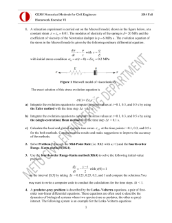


© Copyright 2026