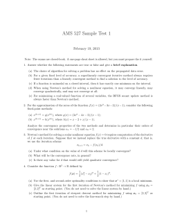
Frequency-domain adaptive iterative image
restoration and evaluation of the regularization
parameter
Moon Ci Kang
Aggelos K. Katsaggelos, MEMBER SPIE
Northwestern University
McCormick School of Engineering and
Applied Science
Department of Electrical Engineering and
Computer Science
Evanston, Illinois 60208-3118
E-mail: [email protected]
Abstract. An important consideration in regularized image restoration is
the evaluation of the regularization parameter. Various techniques exist
in the literature for the evaluation of this parameter, which depend on
the assumed prior knowledge about the problem. These techniques eval-
uate the regularization parameter either at a separate preprocessing
step or by iterating based on the completely restored image, therefore
requiring many restorations of the image with different values of the re-
gularization parameter. The authors propose a nonlinear frequencydomain adaptive regularized iterative image restoration algorithm. According to this algorithm a regularization circulant matrix is used that
corresponds to the assignment of a regularization parameter to each
discrete frequency. Therefore, each frequency component is appropriately regularized. The resulting algorithm produces more accurate resuits and converges considerably faster than the algorithm that uses one
regularization parameter for all frequencies. The regularization matrix is
updated at each iteration step, based on the partially restored image. No
prior knowledge about the image or the noise is required. The development of the algorithm is based on a set-theoretic regularization approach, where bounds on the weighted error residual and stabilizing
functional are updated in the frequency domain at each iteration step.
The proposed algorithm is analyzed theoretically and tested experimen-
tally. Sufficient conditions for convergence are obtained in terms of a
control parameter, which is specified by the conditions for convergence
and optimality of the regularization parameters at each discrete frequency location. Finally the proposed algorithm is compared experimentally with other related algorithms.
Subject terms: digital image recovery and synthesis; image restoration; regularization; iterative algorithms.
Optical Engineering 33(10), 3222-3232 (October 1994).
1 Introduction
A number of techniques providing a solution to the image
restoration
problem have appeared in the literature.1'2 A clasDueto the imperfection of physical imaging systems and the
sification of the major restoration approaches can be found,
particular physical limitations imposed on every application
for example, in Chapter 1 of Ref. 2. Most existing image
where image data are recorded, a recorded image represents
a noisy and blurred version of an original scene in many
practical situations. The blur may be, for example, due to
motion, incorrect focusing, or atmospheric turbulence, while
the noise may originate from the image formation process,
the transmission medium, the recording process, or any combination of these. The goal of image restoration is to recover
the original scene from the degraded observations. Image
restoration techniques are oriented toward modeling the
degradiations, blur, and noise, and applying an inverse procedure to obtain an approximation of the original image.
Paper DIR-Ol received Mar. 2, 1994; accepted for publication June 27, 1994.
1994 Society of Photo-Optical Instrumentation Engineers. 0091-3286/94/$6.OO.
3222/OPTICAL ENGINEERING/October 1994/Vol. 33 No.10
recovery or restoration methods have a common estimation
structure, in spite of their apparent variety. This common
structure is expressed by regularization theory. Qualitatively
speaking, the underlying idea in many regularization approaches is the use of prior information on the solution or
the parameters to be estimated. This prior information is
combined with the data information and defines a solution
by trying to achieve smoothness and yet remain ''faithful"
to the data.
The parameter that controls the trade-off between fidelity
to the data and smoothness of the solution is called the regularization parameter. Its selection is very critical to the
overall quality of the restored image. Various approaches
exist for evaluating this parameter. Some of these require
FREQUENCY-DOMAIN ADAPTIVE ITERATIVE IMAGE RESTORATION
knowledge of the noise variance,35 and some do not (crossvalidation,4'6 maximum likelihood4). All of these approaches
either require the completely restored image based on a value
of the regularization parameter—in order to appropriately
adjust the new value of the regularization parameter (resulting
in considerable computational overhead)—or treat the evaluation of the regularization parameter as a completely separate initial step. In Refs. 7 and 8 iterative algorithms were
introduced and analyzed that evaluate the regularization parameter simultaneously with the restored image, thereby removing the disadvantages of excessive computational load
and/or the need for knowledge of the noise variance of existing techniques.
Another disadvantage of existing nonstochastic regularization techniques is the use of a single scalar regularization
parameter. Its selection, although it is based on an optimality
criterion, represents a compromise between regions that need
turbation in the solution. A regularization approach replaces
an ill-posed problem by a well-posed problem whose solution
is an acceptable approximation to the solution of the given
ill-posed problem.'2
to be overregularized and regions that need to be under-
(3)
regularized. Spatially adaptive techniques provide a solution
to the restoration of images that are nonstationary in nature,
by still using a single regularization parameter but adapting
91
the smoothness
In this paper we introduce adaptivity into the restoration
process by using a constant smoothness constraint, but assigning a different regularization parameter at each discrete
frequency location. We can now ' 'fine-tune' the regularization of each frequency component, thereby achieving more
'
desirable restoration and at the same time speeding up the
convergence of the iterative algorithm used for obtaining the
restored image. We evaluate the regularization parameters
simultaneously with the restored image (based on the partially
restored image), by extending the results in Refs. 7 and 8.
The derivation of the algorithm is based on a set-theoretic
regularization approach, as explained in Sec. 2. The convergence analysis of the proposed iterative algorithm is presented in Sec. 3. The analysis of the singular points of the
blurring function is shown in Sec. 4. Finally, experimental
results and conclusions are given in Secs. 5 and 6, respec-
(2)
XEQX
where Q is a set of signals with certain known properties.
The knowledge we want to express by constraining x to Q
is that the solution is smooth. This is achieved by defining
Q by
Q={xI fCxfI2E2}
where (I.f( denotes the 12 norm, E is a prescribed constant, and
C is a linear operator that has high-pass characteristics. Similarly, the prior information constrains the zero-mean noise
n to an ellipsoid Q, given by
nnQ{n( 11n112<E2}
(4)
where E is an estimate on the data accuracy (noise norm).
Since n lies in a set, it follows that a given observation y
combines with the set Q to define a new set that must contain
x. Thus the observation y specifies a set Q that must contain
x, i.e.,
XEQ,dY{X(y—DX)EQfl}
(5)
Since each of the sets Q, and Q,, contains x, it follows that
x must lie in their intersection. The center of one of the
ellipsoids that bounds their intersection is chosen as a solution.'°'1' It is given by
(DTD+oCTC)x=DTy,
tively.
(6)
(/)2
2 Frequency-Adaptive Regularization
2.1 Formulation
The image degradation process can be adequately modeled
by a linear blur and an additive white Gaussian noise process.'
Then the degradation model is described by
y=Dx+n
With the set-theoretic approach,'°"3 the prior knowledge constrains the solution to certain sets. The sets to be
used are ellipsoids. Therefore, consistency with all the prior
knowledge pertaining to the original image serves as an estimation criterion. More specifically, it is assumed that
(1)
where the vectors y, x, and n represent, respectively, the
lexicographically ordered noisy blurred image, the nonstochastic original image, and the additive noise. The matrix D
represents the linear spatially invariant distortion. The image
restoration problem calls for obtaining an estimate of x given
y, D, and possibly some knowledge about the noise process.
If the image formation process is modeled in a continuous
infinite-dimensional space, Eq. (1) becomes a Fredholm integral equation of the first kind. Then the solution of Eq. (1)
is almost always an ill-posed problem.'2 This means that the
unique least-squares solution of minimal norm of Eq. (1)
does not depend continuously on the data, or that a bounded
perturbation (noise) in the data results in an unbounded per-
where ci =
is the regularization parameter. A posterior
test is actually required to make sure that indeed the solution
of Eq. (6) satisfies both Eqs. (3) and (4).
As already mentioned in the introduction, in this work we
propose an adaptive form of Eq. (6) by using a regularization
matrix instead of a scalar regularization parameter a. More
specifically, we propose to use the following two ellipsoids
Q and Q, in a weighted space:
Q={xJ JICxIJRER}
(7)
Q={x Iy—DxE}
(8)
where P and R are both block-circulant weighting matrices.
Then a solution that belongs to the intersection of Q and
is given by
(DTPTPD+XCTRTRC)iz= DTPTPy,
(9)
where X = (p/ER)2. Let us define P Tp B, R = P0, and
XQ TQ A. Then Eq. (9) can be written as
(D TBD + CTBAC)i = DTBy,
(10)
OPTICAL ENGINEERING I October 1994 I Vol. 33 No. 10 I 3223
KANG and KATSAGGELOS
or
X0(i)=p(i)D*(i)Y(i)
B(DTD+ACTC)=BDy ,
—
(11)
since all matrices are block-circulant and they therefore corn-
Xk+ 1
=
mute. The regularization matrix A is defined based on the
set-theoretic regularization as
A= My— Dx112(fICxfI2I + A)
(12)
is a block-circulant matrix used to ensure convergence, and I is the identity matrix; B plays the role of the
'
'
'shaping' matrix'4 for maximizing the speed of convergence at every frequency component, as well as for cornpensating for the near-singular frequency components, as will
be described in the following sections.
where
2.2 Proposed Iterative Algorithm
There are a number of ways for solving Eqs. (6) and (10)
D(rn)Xk(rn)2
— 13(/)mI()
flIC()Xk(2
+ ik(l) C(i){2) Xk(l)
(1
+13(i)D*(i)[Y(i)_D(i)Xk(i)]
(17)
According to this iteration, since 13 and Sk are frequency
dependent, the convergence of the iteration can be accelerated, as will become clear from the analysis in the following
sections.
3 Optimality and Convergence
In this section we first determine the allowable range of each
regularization and control parameter in the discrete frequency
domain. This is achieved by considering the minimization of
when the regularization parameter is known."2 For example,
E[IIx — i(A)112]
a direct solution in the discrete frequency domain can be
where E['] denotes the expectation operator, and (A) the
obtained, since the matrices D and C are assumed to be block
circulant. However, if the regularization parameter is not
known, and also for incorporating prior knowledge about the
original image into the solution, iterative algorithms can be
employed. Iterative algorithms have been analyzed in detail
in Refs. 10 and 1 1 when a, or both bounds E2 and E2 in Eqs.
(3) and (4), respectively, are known, when only one bound
E2 is known,7 and when no bound is known.8
solution of Eq. (1) as a function of A. Following a procedure
similar to the one described in Ref. 8, we obtain the following
optimal range of a(l) and i(l) at every discrete frequency
location (see Appendix):
= iIY() — D(rn)(m)I2
— <a
N2 max1(IX(i)121C(i)12)
In order to obtain a solution to Eq. (10), successive approximations are used in Refs. 10, 15, and 16, resulting in
Xk± I
Xk +
B[DTy (DTD + AkCTC)xkl '
(18)
N2 1Y(m)
<—
N2
—
D(m)(m)J2
where Ak= IIY — DxkII2[fICxkJI2I + kI '. It is mentioned here
that the iteration (13) can be also derived from the regularized
and
equation
0 < kopt(l)N2max (Xk(l)2C(l)2)
(DTD + ACTC)i = DTy ,
(14)
by using the generalized Landweber's iteration.'4 Since all
matrices in the iteration (13) are block-circulant, the iteration
can be written in the discrete frequency domain as
X0(i) = p(i)D*(i)Y(i) ,
Xk+ '(P
Xk(l) + p(i)[D*(i)Y(i)
(15)
where = ('1"2)' 0l1N— 1, 0l2N— 1, Xk+ 1(1) and
Y(i) represent the two-dimensional (2-D) DFT of the unstacked image estimate Xk± and the noisy blurred image y,
and D(i), C(i), 13(l), and ak(l) represent 2-D DFTs of the
2-D sequences that form the block-circulant matrices D, C,
B, and Ak, respectively. Since k is block-circulant, ak(l) is
given by
I \2
m ') I'?!\ ak(l)
'
ak) flIC(n)Xk( +
Vf "
km)
—
—
—
—
C(m)Xk(m)2 = pt
(20)
,
where a0(L) and akopt(l) are the values that minimize (18).
We turn now to the analysis of the convergence of
the frequency-domain adaptive algorithm. The algorithm has
more than two fixed points. The first fixed point is the inverse
—(ID()I2+ak()IC()I2)Xk(PI
'V
(19)
min1(JX(/)121C(i)12)
(13)
''16)
-
where k(L) is the 2-D DFT of the sequence that forms k•
Therefore, the proposed iteration takes the form
3224 / OPTICAL ENGINEERING / October 1994 / Vol. 33 No. 10
or generalized inverse solution of Eq. (1). Clearly, if D is
invertible, then X(i) = Y(i)/D(i) is a fixed point of the iteration (17), as is easily verified. If D is not invertible, then
solutions that minimize y — Dx112, that is, satisfy D(i)12
X(i) = D*(i)Y(i), are also fixed points of the iteration (17).
For the frequencies for which D(i) = 0, the solution X(l) = 0
is obtained, which is the generalized inverse solution The
second type of fixed points are regularized approximations
to the original image. Since more than one solution exists
to the iteration (17), the determination of the initial condi-
tion becomes important. As shown in Sec. 5, it has
been verified experimentally
that if a ' 'smooth' ' image is
.
.
.
used for X0(i), almost identical fixed points result, independently of X0.
Sufficient conditions for the convergence of the iteration
(17) are derived now, based on the assumption that Xk(l) is
in the vicinity of a fixed point and on the validity of the
FREQUENCY-DOMAIN ADAPTIVE ITERATIVE IMAGE RESTORATION
- 2jY(n) — D(n)Xk(n)I2C(l)I4Xk(l)I2
resulting approximations. The frequency iteration (17) can
be rewritten as
Xk+ 1(f) = Xk(l) + 3(i)[D*(i)Y(i)
(21)
—ID()2Xk()—F(Xk())I
where the frequency nonlinear factor F (Xk(l)) is equal to
F(Xk(l))=
m'(m) — D(rn)Xk(rn)2C(l)2Xk(l)
[rnC(rn)Xk(rn)2 + k(1)I
: Y(n)Hl—Dl2+
k
Xk±
()
—
Xk(l) = [1 — 3(l)D(l)2I[Xk(l) — Xk_ ()I
- 2Y(n)—D(n)Xk(n)2C(l)I4Xk(1)I2
+ k(1)1
.
—
1 (01
+ 0(h2) ,
where Mk(l) = 2/Hk(l). A lower bound for Mk(l) independent of the iteration step k is given by
2
'
(30)
M(i) —
D(i)2 +
(24)
where min(L) 5 the minimum value over all iterations at a
frequency I (also discussed in Sec. 5). The bound M(l) is
where F '(Xk(l)) is the derivative of F(Xk(l)) with respect to
Xk(l), and 0(h2) is the second-order zero term ofthe iteration
step Xk(l) — Xk_ (L) at frequency . In Taylor's expansion
(24), we have assumed that the factor Xk(l) — Xk_ 1(L) is very
small (first-order zero function); therefore the term Y2[Xk(l)
—
Xk_ l(l)]2F"(Xk(l)), where F' denotes the second derivative of F, has been omitted. Using Eq. (24), Eq. (23) becomes
Xk+ 1(1) — Xk(l)
[1
-
\\
—
2,jY(n) —
strictly positive, since 0D(i)I1 and 0C(i)lE1, and
therefore a f3(l) satisfying 0 < 3(l) < M(l) can always be
found at every frequency component.
The condition Hk(l) > 0 is used in establishing a bound
Ofl k(L); it can be rewritten as
fD(l)2k(l)2+
=
[
r
-
D(n)Xk(n)2C(i)2]k(i)
/
\2
+ [D(l)2(fC(rn)Xk(rn)2) +fY(n)
+ k(1))
(25)
—
If we consider the magnitudes of both sides of Eq. (25), we
obtain with the use of the triangular inequality
—
[2D(l2C(rn)Xk(rni2
+ IYQ)
rn C(rn)Xk(rn)2 + k(')
X[Xk(l)—Xk_J(l)I .
(29)
,
(23)
F(Xk(l)) = F(Xk_ 1 (1)) + F '(Xk(l))[Xk(l)
- 2 Y(n) - D(n)Xk(n)2IC(i)2C(i)Xk(i)2] .
Xk(l)
—
.,jY(n) — D(n)Xk(n)2C(l)2
1—
(28
[C(rn)Xk(rn)I2
O<13(l)<Mk(l)
According to the Taylor series expansion,
()
--
D(n)Xk(n)2C(l)I2
-
should be strictly positive, and 3(l) should satisfy
—3(l)[F(Xk(l))—F(Xkl(l))J
Xk±
—
jC(rn)Xk(rn)12 + k(l)
Rewriting the iteration (21) for two consecutive values of k,
we obtain
(27
is sufficient for the convergence of the iteration. In order for
the inequality (27) to be satisfied, Hk defined as
(22)
.
<
The
(31)
condition for k(l) is
m(m)Xk(m)2 + k(')
2Y(n) —
—
21 D(l)12 .jC(rn)Xk(rn)l2 — IY()— D(n)Xk(n)121C(l)12
(rnC(m)Xk(m)2 + k(1))
XXk(l)—Xk_l(l) .
'
(26)
C(l)l
[
/
21D(i)12
+ 21D(1)12[ C(i)l2
Y(n) D(n)Xk(n)12)2
According to (26) the condition
1 °'P'/D'l2+
Y(n)
— D(n)Xk(n)f2IC(l)2
—
——
—
C(m)Xk(m)I2+k(l)
V2
+ 8lD(l)l2lC(l)Xk(l)l2lY(n) —
D(n)Xk(n)12]
COflV(/) .
(32)
OPTICAL ENGINEERING / October 1994 / VoL 33 No. 10/3225
KANG and KATSAGGELOS
Overall, if 0 < 13(1) <M(l) and Eq. (32) is satisfied, the iteration (17) converges. Henceforth, we denote by sed(1)
the k(l) used in the iteration (17).
1.6e+13
1.4e+13
1.2e+13
4 Analysis of Singular Points of D(i)
le+13
Two conditions have been derived for k(l): Eq. (20), which
is based on an optimality criterion, and Eq. (32), resulting
from the convergence analysis of the iteration. If both conditions are satisfied, then
(Sk(L$e+12
6e+12
4e+12
(33)
2e+12
A used(1) satisfying (33) can be found for almost all discrete
frequencies L. However, the lower bound 8"(i) becomes
0
COflV(l)<USed(l)<OPt .
5
greater than the upper bound Pt for frequencies 1 in the
neighborhood of the singular or near-singular points of
(a)
2.5e+13
D(i), due to the division by D(i) in Eq. (32). The behavior
of the algorithm at three types of frequency regions is examined next.
4.1
10
Nuiiiber of iterations
2e+13
Nonsingular-Point Region
1.5e+13
This is the region defined by the discrete frequencies 1 for
which
'5k (Li
le+13
COflV(l)<SOPt .
(34)
In this case a ''(i) was used, as defined by the relation
ased(i) = COflV(i) + .y[Pt — oflv(i)I ,
(35)
0
10
0< y < 1. The values of tised
and mjfl for an
arbitrary frequency location 1= (O.71T, O.75'rr) are shown in
Figs. 1(a) and 1(b) for SNRs of 20 and 30 dB, respectively.
Such a frequency location belongs to the nonsingular-point
region.
where
5e+12
Number of iterations
(b)
Fig. 1 Comparison of sed, opt and min with a uniform blurred image (7 x 7) for: (a) SNR = 20 dB at an arbitrary frequency component
and (b) SNR = 30 dB at an arbitrary frequency component, at an
arbitrary frequency (O.7-rr, O.75'rr).
4.2 Exact-Singular-Point Region
Let us now consider the frequencies 1 * for which D(i * ) 0.
and therefore ak(1 * ) 0.
At these frequencies k(1 'K )
It is this relationship that defines the near-singular-point re-
Since according to Eq. (17) we have X0(i) = 3(i)D *(i)
gion. In this region, unlike the exact-singular-point region,
x is not zero. It is instead very close to the inverse solution,
Y(i), it holds that X0(i*) 0. Furthermore, according to the
iteration (17),
since ak(l) is very small due to the very large value of
Xl(l*)=Xo(l*)+13(l*)[D*(l*)Y(l*)_cxk(l*)Xk(l*)]
In this region, in order to avoid the inverse solutions,
spectral filtering is used. By setting KTK= (DTD + ACTC)
and D T = KTg, the Moore-Penrose pseudoinverse solution17
of Eq. (14) is written as
= X0(i *) = 0
,'
X(l*)=X0(l*)=0
(36)
From the above analysis we see that at the set of frequencies
1*, the generalized inverse solution is obtained, that is,
X(i*) = 0, according to Eq. (36).
As is clear from Eq. (32), for values of D(i) close to zero
the resulting values of oflV(1) become very large. For these
frequencies it turns out that
Pt
(38)
where cr , v, , and u denote respectively the singular value
of K and the left and right singular vectors of K, and p is the
rank of K.
The spectral filtering solution is then expressed as14'8
4.3 Near-Singular-Point Region
COflV(i) >
=:—'—-.
i=1°j
XSF =
s(o) -'- v1 ,
(39)
where s(cr) = 1 if cry> T and 0 otherwise. In our work we
(37)
3226 / OPTICAL ENGINEERING / October 1994 / Vol. 33 No. 10
propose to determine 'r by the condition (37). With this simple
FREQUENCY-DOMAIN ADAPTIVE ITERATIVE IMAGE RESTORATION
spectral-filtering function, the frequency components in the
near-singular-point region are treated the same as with the
exact singular points. We now include the spectral filtering
function B in Eq. (14) following a procedure similar to
Strand' 14 Returning to the iteration (13), the restored result
at the k'th iteration with zero initial condition is given by
Xk=
I
BKTK
=iLrI_(I_BKTK)k]U1Tg
(40)
Here, B is restricted to have the same set of eigenvectors as
KTK, that is,
(41)
Bv1==p,v,
where X1 = a- and we assume that O<p1 X1 <2 for all i. Furthermore, B = F (KTK), where F (X) is a rational fraction and
0< XF(X) <2, for all X. Then Eq. (40) becomes
Xk=
P
T
i=1
a-i
UT
=Rk(Xj)-—-vj
(T
(42)
Equation (43) has the form of Eq. (39); in other words, Rk
(X1) should approximate the spectral filtering function s(a-).
There are a number of ways to approximate the step truncation
function of s(o-1) with the polynomial X[1 — (1 —pX)'i. One
way is the minimization of the ripple energy in both the stop
band and the passband. In other words, define a polynomial
of order m,
P(X)=XF(X)=a1X+a2X2+..- +amXm
(45)
and minimize the ripple energy
rT
E(T) j P2(X) dX + j [1 — P(X)12 dX
0
-r
(47)
In order for (l) to satisfy the sufficient condition for convergence of the iteration (29), the values of M(l) in Eq. (30)
need to be determined, so that the condition 0 < 3(l) <M(l)
is verified at each iteration step. For the determination of
M(l), the minimum value of 1sed(1) over all iterations, denoted by min(L)' needs to be known, where sed(1) is defined
in Eq. (32) and y = 0.5 is used. Toward that end, the value
of s(i) estimated from Eq. (32) is set equal to min(L). If
c(L) < ised(1) then l) is set equal to min(L). In all
our experiments, it was observed that min(L) was reached
after a small number of iterations. In Figs. 2(a) and 2(b), the
plots of 13(1) and M(l) — 3(l) are shown, respectively. Since
M(l) — 13(1) is positive at all frequencies, 3(l) is less than
the convergence bound M(l) at all frequencies, and therefore
the sufficient condition for convergence is satisfied.
The performance of the restoration algorithm was evaluated by measuring the weighted improvement in signal-tonoise ratio defined in decibels by
—
SNR10 log10
(44)
(46)
Therefore, B is a polynomial of D TD with coefficient a,
1443.75D(i)4— 34651D(i)16
+ 4504.5D(i)I8 — 30031D(i)f'° + 804.375ID(i)'2
(43)
where
Rk(X)= 1 —(1 _pX)k
= 31.5 — 315ID(i)2+
I Xorig
2
Cong p
X0fl11
(48)
where Xong denotes the original image, which is available in
a simulation, and
the restored image at convergence.
The weighting matrix P is defined in Eq. (9) and satisfies
pTp B [an example of B is shown in Fig. 2(a)]. Since P
is a high-pass filter, the high-frequency content of the flumerator and denominator quantities in Eq. (48) is weighted
heavier. This is in agreement with the objectives of the adaptive filter we propose. We believe that the metric in Eq. (48)
better represents the quality of the image restored by the
proposed and nonadaptive algorithms. The values of LNR
and the required number of iterations, as well as the estimation of the variance of the noise, a- = y — DxklI2/N2 at
convergence, are shown in Table 1 for SNRs of 20 and 30
dB with a uniformly blurred image, for the proposed algorithm as well as for the algorithm in Ref. 8, which uses one
regularization parameter for the whole image. From this cornparison the proposed algorithm reaches convergence considerably faster than the algorithm in Ref. 8, and also results in
obtained as outlined above. The detailed procedure of deriving the spectral filtering function is shown in Ref. 14.
a sharper image in terms of the metric LNR and according
to visual inspection.
The values of the residual y — DxkII2/N2 and of the error
5 Experimental Results
between iteration steps, IIXk — Xk_ 112, for the two SNRs men-
The performance of the proposed frequency-domain iterative
restoration algorithm is illustrated with artificially blurred
images obtained with a 7 X 7 uniform point-spread function
(PSF). Some of these results are presented in this section,
where a 256- x 256-pixel portrait image was used, the 2-D
—
Laplacian was used for C, and the criterion
Xk112/
106
was
used
for terminating the iteration; 3(l),
IIXkII2
which is obtained from the analysis of the singular points
with T = 0.007, is given by'4
13(i) = F (ID()I2)
tioned above are compared in Figs. 3 and 4, respectively.
Notice that the plots are scaled appropriately and that the
vertical axis in Fig. 4 is logarithmic. It is observed in Fig. 3
that in all cases the residuals converge to a value close to but
slightly smaller than the true values. This result is expected,
since the solution at convergence [center of an ellipsoid
bounding the intersection of Q and Q in Eqs. (3) and (5),
respectively] lies inside the ellipsoid Q,,. The plots in Figs.
3 and 4 demonstrate that in all cases the iterative algorithm
converges at the same rate. The noisy blurred images are
shown in Figs. 5(a) and 5(c) for SNRs of 20 and 30 dB. The
corresponding restored images are shown in Figs. 5(b)
OPTICAL ENGINEERING/October 1994/Vol. 33 No. 10/3227
KANG and KATSAGGELOS
(a)
4
2.5)<10
4
2.0>(10
x1 0
0
4
4
3
5.0)<10
(b)
Fig. 2 (a) Values of 13(I) from singular-point analysis; (b) values of M(!) — 13(1).
3228 / OPTICAL ENGINEERING / October 1994 / Vol. 33 No. 10
FREQUENCY-DOMAIN ADAPTIVE ITERATIVE IMAGE RESTORATION
Table 1 SNR improvement and estimated variance of noise for various SNRs with a uniform blurred image.
- SNR
SNR # of iteration Estimated variance of noise
frequency adaptive algorithm: with regularization matrix
11
17.90
20 dB 4.7 dB
30 dB 5.6 dB
14
1.871
iteration adaptive algorithm: with one regularization parameter
20 dB 4.2 dB
30 dB 4.9 dB
18.21
89
75
1.902
a,= 22.70 at 20 dB and 2.270 at 30 dB
of the noise (which is estimated by the algorithm) or the
degree of smoothness of the solution. The partially restored
image is used in extracting the required information. Sufficient conditions for the convergence of the algorithm have
been derived in the frequency domain. Spectral-filtering resuits have been used in handling the near-singular-point region and in speeding up the convergence of the iteration.
Linear constraints can also be incorporated into the iteration.
When nonlinear constraints are used, the linearization step
in the analysis of the algorithm cannot be applied, although
the algorithm has been shown to converge experimentally.
7 Appendix
100
In this appendix, an analysis is presented of the error between
the original image and the regularized estimate, following
Refs. 4 and 8. It leads to the determination of an optimal
range for the parameter k(l) in Eq. (16). Let us denote by
80
60
x the minimum-norm least-squares solution of Eq. (1), that
is, x = (D
D Ty Then the regularized solution (A)
can be written as
Residual
40
(A)=(DTD + ACTCy 1DTy
20
(49)
=(DTD+ACTC)'DTDx
(50)
=P(A)x
(51)
0
10
5
Number of iterations
Fig. 3 Values of IIY — Dxkll2/N2 with a uniform blurred image for
SNR=20 dB and 30 dB.
where P (A) = (DTD + ACTC)_ 1DTD. The mean squared
error (MSE) is given by
(52)
E[Ifx — (A)Il2]
E[fIe(A)112]
=E[(x x)TP(A)TP(A)(x —x)]
(53)
where E[.] denotes the expectation operator. Since
E [(A)I = P(A)x, the first term of Eq. (53) is equal to the
variance of i(A), while the second term is equal to the bias
of the estimate i. Since D and C are block-circulant matrices,
the variance and bias term in Eq. (53) can be described in
the discrete Fourier transform (DFT) domain as
N2
10
Number of iterations
Fig. 4 Values of IIXk—Xk_1112 with a uniform blurred image for
SNR=20 dB and 30 dB.
Var[(A)] =
(Iv(rn)
—
D(rn)X(rn)12)
ID(l)12
xIE
\1=:l [ID(i)12+a(i)IC(i)12121 ,
fN2
1
(&NR 4.7 dB) and 5(d) (NR 5.6 dB). In all cases the
restored images are very satisfactory, according to the improvement in SNR and visual inspection.
6 Conclusions
In this paper we have proposed a regularized iterative image
restoration algorithm according to which a restored image
and an estimate of the regularization matrix are provided
simultaneously at each iteration step. Since the regularization
matrix is chosen to be block circulant, the regularization is
adapted to the parameters of each discrete frequency component. No prior knowledge is required about the variance
(54)
N2 IX(l)I2a(l)2IC(l)4
bias[x(A)}=
'
(55)
[ID()I2+a()C()I212
where L=: (11,12), i= (m1,m2), with OEl1 N— 1, Ol2E
N— 1, Om1 N— 1, Om2N— 1, X(i) and Y(rn) represent the 2-D DFTs of the unstacked image estimate i and the
noisy blurred image y, and D(i) and C(i) represent 2-D DFTs
of the 2-D sequences that form the block-circulant matrices
D TD and C Tc respectively. Taking their derivatives with
respect to ci() yields
OPTICAL ENGINEERING / October 1994 / Vol. 33 No. 10 I 3229
KANG and KATSAGGELOS
(a)
(b)
(c)
(d)
Fig. 5 Noisy blurred and restored images for 7x7 uniform blur: (a) SNR=20 dB, noisy, blurred;
(b) SNR=20 dB, restored image; (c) SNR=30 dB, noisy, blurred; (d) SNR=30 dB, restored image.
3230 / OPTICAL ENGINEERING / October 1994 / Vol. 33 No. 10
FREQUENCY-DOMAIN ADAPTIVE ITERATIVE IMAGE RESTORATION
a Var[i(A)J
8a()
= 2(—-- : IY(m) N2rn1
x
3a()
ID(PI2IC(l)12
(
Y(n) — D(n)Xk(n)12
D(m)X(m)12)
<O
N2
a bias[i(A)J
Since
N2
ak(l)(C(m)X(rn)(2+(1) ,
,
(56)
we obtain from Eq. (61) that
O<kOPt(l)N2 max[Xk(l)I2fC(l)21
N2
a(l)IX(l)J2C(l)4D(l)2>°
L=' [D(i)I2+c(i)C(i)I2]3
=2
1
(57)
.
m
From Eqs. (54) and (56) we conclude that the variance is a
strictly positive, monotonically decreasing function of a(l)
for a(1) > 0 and that Var(oo)] = 0. Similarly, from Eqs. (55)
and (57) we conclude that the bias is a positive, monotonically
increasing function ofa(l) for a(l) > 0 and that bias[(O)] = 0
and bias[i(oo)I = 11x112. Thus, the total error as a function of
ci(L) is the sum of a monotonically decreasing and a monotonically increasing function ofa(l). Therefore, the MSE has
either one minimum or one maximum for 0 <a(l) < oo The
derivative of the MSE with respect to a(l) is equal to
8E[IIe(A)112] =
8a()
x
2
N2
D(l)121C(l)12
—
<0
m
=I
for 0 <a(l)
<
- N2
Y(m) — D(m)X(m)2
max1[X(/)2C(l)2]
'
N2
m= 1
Y(m) — D(m)X(m)2
>0 for —
N2 min1[fX(i)(2C(i)2 I
<c(l)<oc .
(60)
Therefore, according to the conditions (56), (57), (59), and
(60), the MSE function has a unique minimum for 0 < c(1)
< 00; this minimum is attained by the value aOP(l)' which is
in the range
:
=1
M. E. Zervakis and T. M. Kwon, "Robust estimation techniques in
regularized image restoration," Opt. Eng. 29(5), 455-470 (May 1990).
6. 5. J. Reeves and R. M. Mersereau, ' 'Optimal estimation of the regularization parameters and stabilizing functional for regularized image
restoration," Opt. Eng. 29, 446-454 (May 1990).
7. M. G. Kang and A. K. Katsaggelos, ' 'Simultaneous iterative image restoration and evaluation of the regularization parameter,' ' IEEE Trans.
Signal Processing 40, 2329—2334 (Sep. 1992).
(59)
8a()
i. H. C. Andrews and B. R. Hunt, Digital Image Restoration, PrenticeHall, New York (1977).
2. A. K. Katsaggelos, Ed., Digital Image Restoration, Springer Series in
Information Sciences, Vol. 23, Springer-Verlag, Heidelberg (1991).
3. B. R. Hunt, ' 'Application of constrained least squares estimation to
image restoration by digital computers," IEEE Trans. Comput. C-22,
8. A. K. Katsaggelos and M. G. Kang, ' 'Iterative evaluation of the regularization parameter in regularized image restoration,' ' J. Visual
N2
8E[Ile(A)I2J
References
5.
Therefore,
8a()
Telescope Science Institute, Baltimore, Maryland.
332—336 (July 1992).
.
IY()— D(rn)X(m)12
—
)
(58)
8E[IIe(A)112]
Acknowledgment
This work is supported in part by a grant from the Space
805—812 (1973).
N2
(aII2cI2
(63)
4. N. P. Galatsanos and A. K. Katsaggelos, "Methods for choosing the
regularization parameter and estimating the noise variance in image
restoration and their relation,' ' IEEE Trans. Image Processing 1,
[lD()I2 a(1)C(1)2I3
N2m = 1
(62)
Comm. and Image Rep. 3(6), 446—455 (Dec. 1992).
9. A. K. Katsaggelos, "A general formulation of adaptive iterative image
restoration algorithms,' ' in Proc. 1986 International Conf on Acoustics, Speech, Signal Processing, pp. 42—47 (Mar. 1986).
10. A. K. Katsaggelos, ' 'Iterative image restoration algorithm,' ' Opt. Eng.
28(7), 735—748 (July 1989).
I 1. A. K. Katsaggelos, J. Biemond, R. W. Schafer, and R. M. Mersereau,
' 'A regularized iterative image restoration algorithm,' ' IEEE Trans.
Signal Processing 39, 914—929 (Apr. 1991).
12. A. N. Tikhonov and V. Y. Arsenin, Solution of Ill-posed Problems,
V. H. Winston and Sons, Washington, DC (1977).
13. F. C. Schweppe, Uncertain Dynamic Systems, Prentice-Hall, Engle-
woodCliffs,NJ (1973).
14. 0. N. Strand, ' 'Theory and methods related to the singular function
expansion and Landweber's iteration for integral equation of the first
kind," SIAM J. Numer. Anal. 11, 798-825 (Sep. 1974).
15. R. W. Schafer, R. M. Mersereau, and M. A. Richards, ' 'Constrained
iterative restoration algorithms," Proc. IEEE 69, 432—450 (Apr. 1981).
16. J. M. Ortega and W. C. Rheinboldt, Iterative Solution of Nonlinear
Equations in Several Variables, Academic Press, New York (1970).
17. A. Ben-Israel and T. N. E. Greville, Generalized Inverses: Theory and
Applications, Wiley, New York (1974).
18. B. J. Sullivan and A. K. Katsaggelos, "New termination rule for linear
iterative image restoration algorithm," Opt. Eng. 29, 471—477 (May
1990).
N2
Y(rn) - D(m)X(m)2
—
N2 max1[IX(l)I2C(l)2]
Moon Gi Kang received BS and MS de-
grees in electronics engineering from
<a()
Seoul National University, Korea, in 1986
and 1988, respectively. He received a PhD
degree in electrical engineering from
N2
fY(rn) — D(m)X(m)2
—
<=1
N2 min1[IX(i)121C(i)12]
(61)
Northwestern University in 1994. He was
a research assistant from 1989 to 1993,
and since 1994 he has been working as a
research fellow in the Department of Electrical Engineering and Computer Science
at Northwestern University. His current reOPTICAL ENGINEERING I October 1994 I Vol. 33 No. 10 I 3231
KANG and KATSAGGELOS
search interests include regularized iterative image restoration and
use of higher order spectra for image restoration.
Aggelos K. Katsaggelos received the Diploma degree in electrical and mechanical
engineering from the Aristotelian University of Thessaloniki, Thessaloniki, Greece,
in 1979, and the MS and PhD degrees,
both in electrical engineering, from the
Georgia Institute of Technology, Atlanta,
Georgia, in 1981 and 1985, respectively.
In 1985 he joined the Department of Electrical Engineering and Computer Science
at Northwestern University, Evanston, Illi-
nois, where he is currently an associate professor. During the
1986—1987 academic year he was an assistant professor at Polytechnic University, Department of Electrical Engineering and Com-
3232 / OPTICAL ENGINEERING / October 1994 / Vol. 33 No. 10
puter Science, Brooklyn, New York. His current research interests
include image recovery, processing of moving images (motion estimation, enhancement, very low bit rate compression), and computational vision. Dr. Katsaggelos is an Ameritech Fellow and a member of the Associate Staff, Department of Medicine, at Evanston
Hospital. He is a senior member of the IEEE, and also a member of
the SPIE, the Steering Committees of the IEEE Transactions on
Medical Imaging and the IEEE Transactions on Image Processing,
the IEEE Technical Committees on Visual Signal Processing and
Communications and on Image and Multi-Dimensional Signal Pro-
cessing, the Technical Chamber of Commerce of Greece, and
Sigma Xi. He has served as an associate editor for the IEEE Transactions on Signal Processing (1990—1992), and is currently an area
editor for the journal Graphical Models and Image Processing. He
is the editor of Digital Image Restoration (Springer-Verlag, Heidelberg, 1991) and the general chairman of the 1994 Visual Communications and Image Processing Conference (Chicago).