Algorithms
Lecture 13: Randomized Minimum Cut [Fa’13]
Jaques: But, for the seventh cause; how did you find the quarrel on the seventh cause?
Touchstone: Upon a lie seven times removed:–bear your body more seeming, Audrey:–as
thus, sir. I did dislike the cut of a certain courtier’s beard: he sent me word, if I
said his beard was not cut well, he was in the mind it was: this is called the Retort
Courteous. If I sent him word again ‘it was not well cut,’ he would send me word, he
cut it to please himself: this is called the Quip Modest. If again ‘it was not well cut,’
he disabled my judgment: this is called the Reply Churlish. If again ‘it was not well
cut,’ he would answer, I spake not true: this is called the Reproof Valiant. If again ‘it
was not well cut,’ he would say I lied: this is called the Counter-cheque Quarrelsome:
and so to the Lie Circumstantial and the Lie Direct.
Jaques: And how oft did you say his beard was not well cut?
Touchstone: I durst go no further than the Lie Circumstantial, nor he durst not give me the
Lie Direct; and so we measured swords and parted.
— William Shakespeare, As You Like It, Act V, Scene 4 (1600)
13
13.1
Randomized Minimum Cut
Setting Up the Problem
This lecture considers a problem that arises in robust network design. Suppose we have a
connected multigraph¹ G representing a communications network like the UIUC telephone
system, the Facebook social network, the internet, or Al-Qaeda. In order to disrupt the network,
an enemy agent plans to remove some of the edges in this multigraph (by cutting wires, placing
police at strategic drop-off points, or paying street urchins to ‘lose’ messages) to separate it into
multiple components. Since his country is currently having an economic crisis, the agent wants
to remove as few edges as possible to accomplish this task.
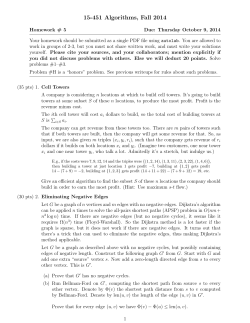
More formally, a cut partitions the nodes of G into two nonempty subsets. The size of the cut
is the number of crossing edges, which have one endpoint in each subset. Finally, a minimum
cut in G is a cut with the smallest number of crossing edges. The same graph may have several
minimum cuts.
a
c
b
d
f
e
g
h
A multigraph whose minimum cut has three edges.
This problem has a long history. The classical deterministic algorithms for this problem rely
on network flow techniques, which are discussed in another lecture. The fastest such algorithms
(that we will discuss) run in O(n3 ) time and are fairly complex; we will see some of these later
in the semester. Here I’ll describe a relatively simple randomized algorithm discovered by David
Karger when he was a Ph.D. student.²
¹A multigraph allows multiple edges between the same pair of nodes. Everything in this lecture could be rephrased
in terms of simple graphs where every edge has a non-negative weight, but this would make the algorithms and
analysis slightly more complicated.
²David R. Karger*. Random sampling in cut, flow, and network design problems. Proc. 25th STOC, 648–657, 1994.
© Copyright 2014 Jeff Erickson.
This work is licensed under a Creative Commons License (http://creativecommons.org/licenses/by-nc-sa/4.0/).
Free distribution is strongly encouraged; commercial distribution is expressly forbidden.
See http://www.cs.uiuc.edu/~jeffe/teaching/algorithms/ for the most recent revision.
1
Algorithms
Lecture 13: Randomized Minimum Cut [Fa’13]
Karger’s algorithm uses a primitive operation called collapsing an edge. Suppose u and v
are vertices that are connected by an edge in some multigraph G. To collapse the edge {u, v},
we create a new node called uv, replace any edge of the form {u, w} or {v, w} with a new edge
{uv, w}, and then delete the original vertices u and v. Equivalently, collapsing the edge shrinks
the edge down to nothing, pulling the two endpoints together. The new collapsed graph is
denoted G/{u, v}. We don’t allow self-loops in our multigraphs; if there are multiple edges
between u and v, collapsing any one of them deletes them all.
a
a
c
d
be
a
b
c
d
b
e
cd
e
A graph G and two collapsed graphs G/{b, e} and G/{c, d}.
Any edge in an n-vertex graph can be collapsed in O(n) time, assuming the graph is
represented as an adjacency list; I’ll leave the precise implementation details as an easy exercise.
The correctness of our algorithms will eventually boil down the following simple observation:
For any cut in G/{u, v}, there is cut in G with exactly the same number of crossing edges. In
fact, in some sense, the ‘same’ edges form the cut in both graphs. The converse is not necessarily
true, however. For example, in the picture above, the original graph G has a cut of size 1, but the
collapsed graph G/{c, d} does not.
This simple observation has two immediate but important consequences. First, collapsing an
edge cannot decrease the minimum cut size. More importantly, collapsing an edge increases the
minimum cut size if and only if that edge is part of every minimum cut.
13.2
Blindly Guessing
Let’s start with an algorithm that tries to guess the minimum cut by randomly collapsing edges
until the graph has only two vertices left.
GuessMinCut(G):
for i ← n downto 2
pick a random edge e in G
G ← G/e
return the only cut in G
Because each collapse requires O(n) time, this algorithm runs in O(n2 ) time. Our earlier
observations imply that as long as we never collapse an edge that lies in every minimum cut, our
algorithm will actually guess correctly. But how likely is that?
Suppose G has only one minimum cut—if it actually has more than one, just pick your
favorite—and this cut has size k. Every vertex of G must lie on at least k edges; otherwise,
we could separate that vertex from the rest of the graph with an even smaller cut. Thus, the
number of incident vertex-edge pairs is at least kn. Since every edge is incident to exactly two
vertices, G must have at least kn/2 edges. That implies that if we pick an edge in G uniformly at
random, the probability of picking an edge in the minimum cut is at most 2/n. In other words,
the probability that we don’t screw up on the very first step is at least 1 − 2/n.
2
Algorithms
Lecture 13: Randomized Minimum Cut [Fa’13]
Once we’ve collapsed the first random edge, the rest of the algorithm proceeds recursively
(with independent random choices) on the remaining (n − 1)-node graph. So the overall
probability P(n) that GuessMinCut returns the true minimum cut is given by the recurrence
P(n) ≥
n−2
· P(n − 1)
n
with base case P(2) = 1. We can expand this recurrence into a product, most of whose factors
cancel out immediately.
P(n) ≥
n
Y
i−2
i=3
13.3
i
Qn−2
(i
−
2)
2
j=1 j
i=3
Qn
= Qn
=
n(n − 1)
i=3 i
i=3 i
Qn
=
Blindly Guessing Over and Over
That’s not very good. Fortunately, there’s a simple method for increasing our chances of finding the
minimum cut: run the guessing algorithm many times and return the smallest guess. Randomized
algorithms folks like to call this idea amplification.
KargerMinCut(G):
mink ← ∞
for i ← 1 to N
X ← GuessMinCut(G)
if |X | < mink
mink ← |X |
minX ← X
return minX
Both the running time and the probability of success will depend on the number of iterations N ,
which we haven’t specified yet.
First let’s figure out the probability that KargerMinCut returns the actual minimum cut.
The only way for the algorithm to return the wrong answer is if GuessMinCut fails N times in a
row. Since each guess is independent, our probability of success is at least

1− 1−
2
n(n − 1)
N
≤ 1 − e−2N /n(n−1) ,
by The World’s Most Useful Inequality 1 + x ≤ e x . By making N larger, we can make
this
n
probability arbitrarily close to 1, but never equal to 1. In particular, if we set N = c 2 ln n for
some constant c, then KargerMinCut is correct with probability at least
1 − e−c ln n = 1 −
1
.
nc
When the failure probability is a polynomial fraction, we say that the algorithm is correct with
high probability. Thus, KargerMinCut computes the minimum cut of any n-node graph in
O(n 4 log n) time.
If we make the number of iterations even larger, say N = n2 (n − 1)/2, the success probability
becomes 1 − e−n . When the failure probability is exponentially small like this, we say that
the algorithm is correct with very high probability. In practice, very high probability is usually
overkill; high probability is enough. (Remember, there is a small but non-zero probability that
your computer will transform itself into a kitten before your program is finished.)
3
Algorithms
13.4
Lecture 13: Randomized Minimum Cut [Fa’13]
Not-So-Blindly Guessing
The O(n4 log n) running time is actually comparable to some of the simpler flow-based algorithms,
but it’s nothing to get excited about. But we can improve our guessing algorithm, and thus
decrease the number of iterations in the outer loop, by observing that as the graph shrinks, the
probability of collapsing an edge in the minimum cut increases. At first the probability is quite
small, only 2/n, but near the end of execution, when the graph has only three vertices, we have a
2/3 chance of screwing up!
A simple technique for working around this increasing probability of error was developed by
David Karger and Cliff Stein.³ Their idea is to group the first several random collapses a ‘safe’
phase, so that the cumulative probability of screwing up is small—less than 1/2, say—and a
‘dangerous’ phase, which is much more likely to screw up. p
The
p safe phase shrinks the graph from n nodes to n/ 2 + 1 nodes, using a sequence of
n − n/ 2 − 1 random collapses. Following our earlier analysis, the probability that none of these
safe collapses touches the minimum cut is at least
p
p
p
n
Y
i − 2 (n/ 2)(n/ 2 + 1)
n+ 2
1
=
=
> .
i
n(n − 1)
2(n − 1) 2
p
i=n/ 2+2
Now, to get around the danger of the dangerous phase, we use amplification. However, instead of
running through the dangerous phase once, we run it twice and keep the best of the two answers.
Naturally, we treat the dangerous phase recursively, so we actually obtain a binary recursion tree,
which expands as we get closer to the base case, instead of a single path. More formally, the
algorithm looks like this:
Contract(G, m):
for i ← n downto m
pick a random edge e in G
G ← G/e
return G
BetterGuess(G):
if G has more than 8 vertices
p
X 1 ← BetterGuess(Contract(G, n/p2 + 1))
X 2 ← BetterGuess(Contract(G, n/ 2 + 1))
return min{X 1 , X 2 }
else
use brute force
This might look like we’re just doing to same thing twice, but remember that Contract (and
thus BetterGuess) is randomized. Each call to Contract contracts an independent random
set of edges; X 1 and X 2 are almost always different cuts.
BetterGuess correctly returns the minimum cut unless both recursive calls return the wrong
result. X 1 is the minimum cut of G if and only if (1) none of the edges of the minimum cut
are Contracted and (2) the recursive call to BetterGuess returns the minimum cut of the
Contracted graph. Thus, if P(n) denotes the probability that BetterGuess returns a minimum
p
cut of an n-node graph, then X 1 is the minimum cut with probability at least 1/2 · P(n/ p2 + 1).
The same argument implies that X 2 is the minimum cut with probability at least 1/2· P(n/ 2+1).
Because these two events are independent, we have the following recurrence, with base case
P(n) = 1 for all n ≤ 6.

2
1
n
P(n) ≥ 1 − 1 − P p + 1
2
2
Using a series of transformations, Karger and Stein prove that P(n) = Ω(1/ log n). I’ve included
the proof at the end of this note.
˜ 2 ) algorithm for minimum cuts. Proc. 25th STOC, 757–765, 1993.
³David R. Karger∗ and Cliff Stein. An O(n
4
Algorithms
Lecture 13: Randomized Minimum Cut [Fa’13]
For the running time, we get a simple recurrence that is easily solved using recursion trees or
the Master theorem (after a domain transformation to remove the +1 from the recurrence).

n
2
T (n) = O(n ) + 2T p + 1 = O(n2 log n)
2
So all this splitting and recursing has slowed down the guessing algorithm slightly, but the
probability of failure is exponentially smaller!
Let’s express the lower bound P(n) = Ω(1/ log n) explicitly as P(n) ≥ α/ ln n for some
constant α. (Karger and Stein’s proof implies α > 2). If we call BetterGuess N = c ln2 n times,
for some new constant c, the overall probability of success is at least
2
1
α c ln n
1− 1−
≥ 1 − e−(c/α) ln n = 1 − c/α .
ln n
n
By setting c sufficiently large, we can bound the probability of failure by an arbitrarily small
polynomial function of n. In other words, we now have an algorithm that computes the minimum
cut with high probability in only O(n 2 log3 n) time!
?
13.5
Solving the Karger-Stein recurrence
Recall the following recurrence for the probability that BetterGuess successfully finds a
minimum cut of an n-node graph:

2
1
n
P(n) ≥ 1 − 1 − P p + 1
2
2
Karger and Stein solve this rather ugly recurrence through a series of functional transformations.
Let p(k) denote the probability of success at the kth level of recursion, counting upward from
the base case. This function satisfies the recurrence

p(k − 1) 2
p(k − 1)2
p(k) ≥ 1 − 1 −
= p(k − 1) −
2
4
with base case p(0) = 1. Let ¯p(k) be the function that satisfies this recurrence with equality;
clearly, p(k) ≥ ¯p(k). Substituting the function z(k) = 4/¯p(k) − 1 into this recurrence implies
(after a bit of algebra) gives a new recurrence
z(k) = z(k − 1) + 2 +
1
z(k − 1)
with base case z(0) = 3. Clearly z(k) > 1 for all k, so we have a conservative upper bound z(k) <
z(k − 1) + 3, which implies (by induction) that z(k) ≤ 3k + 3. Substituting ¯p(k) = 4/(z(k) + 1)
into this solution, we conclude that
p(k) ≥ ¯p(k) >
1
= Ω(1/k).
3k + 6
To compute the number of levels of recursion that BetterGuess executes for an n-node
graph, we solve the secondary recurrence

n
k(n) = 1 + k p + 1
2
with base cases k(n) = 0 for all n ≤ 8. After a domain transformation to remove the +1 from the
right side, the recursion tree method (or the Master theorem) implies that k(n) = Θ(log n).
We conclude that P(n) = p(k(n)) = Ω(1/ log n), as promised. Whew!
5
Algorithms
Lecture 13: Randomized Minimum Cut [Fa’13]
Exercises
1. Suppose you had an algorithm to compute the minimum spanning tree of a graph in O(m)
time, where m is the number of edges in the input graph. Use this algorithm as a subroutine
to improve the running time of GuessMinCut from O(n2 ) to O(m).
(In fact, there is a randomized algorithm—due to Philip Klein, David Karger, and Robert
Tarjan—that computes the minimum spanning tree of any graph in O(m) expected time.
The fastest deterministic algorithm known in 2013 runs in O(mα(m)) time.)
2. Suppose you are given a graph G with weighted edges, and your goal is to find a cut whose
total weight (not just number of edges) is smallest.
(a) Describe an algorithm to select a random edge of G, where the probability of choosing
edge e is proportional to the weight of e.
(b) Prove that if you use the algorithm from part (a), instead of choosing edges uniformly
at random, the probability that GuessMinCut returns a minimum-weight cut is still
Ω(1/n2 ).
(c) What is the running time of your modified GuessMinCut algorithm?
3. Prove that GuessMinCut returns the second smallest cut in its input graph with probability
Ω(1/n3 ). (The second smallest cut could be significantly larger than the minimum cut.)
4. Consider the following generalization of the BetterGuess algorithm, where we pass in a
real parameter α > 1 in addition to the graph G.
BetterGuess(G, α):
n ← number of vertices in G
if n > 8
X 1 ← BetterGuess(Contract(G, n/α), α)
X 2 ← BetterGuess(Contract(G, n/α), α)
return min{X 1 , X 2 }
else
use brute force
Assume for this question that the input graph G has a unique minimum cut.
(a) What is the running time
modified algorithm,
as a function of n and α? [Hint:
p of the p
p
Consider the cases α < 2, α = 2, and α > 2 separately.]
(b) What is the probability that Contract(G, n/α) does not contract any edge in the
minimum cut in G? Give both an exact expression involvingpboth n and α, and a
simple approximation in terms of just α. [Hint: When α = 2, the probability is
approximately 1/2.]
(c) Estimate the probability that BetterGuess(G, α) returns the minimum cut in G,
by adapting
the
p
p solution to
p the Karger-Stein recurrence. [Hint: Consider the cases
α < 2, α = 2, and α > 2 separately.]
6
Algorithms
Lecture 13: Randomized Minimum Cut [Fa’13]
(d) Suppose we iterate BetterGuess(G, α) until we are guaranteed to see the minimum
cut with high probability. What is the running time of the resulting algorithm? For
which value of α is this running time minimized?
(e) Suppose we modify BetterGuess(G, α) further, to recurse four times instead of only
twice. Now what is the best choice of α? What is the resulting running time?
© Copyright 2014 Jeff Erickson.
This work is licensed under a Creative Commons License (http://creativecommons.org/licenses/by-nc-sa/4.0/).
Free distribution is strongly encouraged; commercial distribution is expressly forbidden.
See http://www.cs.uiuc.edu/~jeffe/teaching/algorithms for the most recent revision.
7