1. business and industrial
2. energy
3. coal

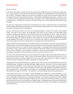
Select Committee on Wind Turbines
Submission 348
CO2 Emissions Savings
from Wind Power in the
National Electricity
Market (NEM)
Submission to the Senate Select Committee on Wind Turbines
Select Committee on Wind Turbines
Submission 348
F INAL R EPORT
PREPARED BY:
D R J OSEPH W HEATLEY
B IOSPHERICA R ISK LTD
COMMISSIONED BY:
A SSOCIATION FOR R ESEARCH OF R ENEWABLE E NERGY IN AUSTRALIA LTD (ARREA)
ABN:65 166 633 263
21 April 2015
Select Committee on Wind Turbines
Submission 348
Contents
1
Executive Summary . . . . . . . . . . . . . . . . . . . . . . . . . . . . . . . . . . . . . . . . . 5
2
Overview of the NEM . . . . . . . . . . . . . . . . . . . . . . . . . . . . . . . . . . . . . . . 7
2.1
renewables
10
2.2
fuel mix
12
2.3
outages
14
2.4
inter-regional flows
15
2.5
emissions
17
3
Empirical Method . . . . . . . . . . . . . . . . . . . . . . . . . . . . . . . . . . . . . . . . . . 20
3.1
emissions models
20
3.2
emissions avoided
22
3.2.1
3.2.2
3.2.3
hydro-wind . . . . . . . . . . . . . . . . . . . . . . . . . . . . . . . . . . . . . . . . . . . . . . . . . . . . . 22
regression . . . . . . . . . . . . . . . . . . . . . . . . . . . . . . . . . . . . . . . . . . . . . . . . . . . . . . 22
peaking plant . . . . . . . . . . . . . . . . . . . . . . . . . . . . . . . . . . . . . . . . . . . . . . . . . . 24
3.3
discussion
25
3.4
limitations and suggested future work
28
4
Additional material . . . . . . . . . . . . . . . . . . . . . . . . . . . . . . . . . . . . . . . . 29
4.1
GLOSSARY
29
Select Committee on Wind Turbines
Submission 348
4
4.2
parameters
32
4.3
emissions avoided by generator
36
4.4
data & references
41
Select Committee on Wind Turbines
Submission 348
1. Executive Summary
This report examines the contribution of wind power to CO2 -e emissions reduction in the NEM in 2014. Using a generation dataset at 5minute intervals, CO2 -e emissions time-series are estimated for each of
151 thermal generators, giving total emissions from fossil fuel plant of
169.7MtCO2 -e. The best empirical estimate is that wind power avoided
6.2MtCO2 -e, a reduction in total emissions of 3.5%. Wind power contributed 4.5% of system demand and therefore the emissions displacement effectiveness of wind power was 3.5%/4.5% or 78% in 2014.
Several factors acted to limit the effectiveness of wind power in reducing emissions in 2014. A significant fraction of South Australia’s wind
output displaced low-emissions gas generation. Wind power tended to
displace black coal plant in New South Wales rather than higher emis-
Select Committee on Wind Turbines
Submission 348
6
sions brown coal plant in Victoria. Part-load inefficiency costs and system losses also degraded effectiveness.
Wind power becomes less effective in displacing emissions from thermal plant as installed capacity increases. The evidence in this study
suggests that effectiveness in the NEM would fall to ≈ 70% if the proportion of energy provided by wind is doubled from 2014 levels.
The emissions parameters for individual power stations available for
this study are approximate, which means that the quantitative results
are subject to increased uncertainty. Data requirements for an improved investigation are described and a detailed multi-year study using such data is warranted.
Select Committee on Wind Turbines
Submission 348
2. Overview of the NEM
De-carbonisation of electricity production is a major goal of environmental policy. Wind
power generation (WPG) is an emissions reducing technology which works by displacing
fossil fuel generation. Unlike renewable sources such as hydro-electric power, WPG is not
dispatchable generation i.e. it is not controlled by the grid operator. Instead the thermal
system must adapt continuously to the natural variability (intermittency) of WPG. As the
complexity of this interaction has become better understood, early optimism about the
efficacy of wind power in emissions reduction has reduced. Under normal priority dispatch
rules for WPG, one unit of wind energy (1 MWh) displaces close to one unit of conventional
generation (slightly less due to system losses). However this relation need not be valid
for CO2 displacement. For instance, wind might selectively displace more flexible, high
marginal cost gas plant rather than baseload coal plant. In that case the displacement
effectiveness1 of WPG is less than unity. In addition to this selective displacement effect,
part-load inefficiency costs, ramping and startup costs tend to become significant as the
installed wind capacity increases. This reduces the effectiveness of wind power in meeting
it’s primary policy goal.
In this report, empirical calculations[1] of the effectiveness of the WPG in the NEM
during 2014 are described. The objective is two-fold:
• determine which information is required to answer this question empirically for the
NEM
• provide estimates of operational emissions savings based on the available data
Operational emissions savings can be defined as the difference between the observed
emissions and what emissions would be in a no-wind scenario all else being equal. This
1 ratio
of % CO2 emissions savings to % WPG, see Section 4.1
Select Committee on Wind Turbines
Submission 348
8
quantity can be investigated empirically. Empirical methods can assess the impact of wind
power on the existing grid but they cannot indicate whether the existing technology mix or
grid configuration is optimal from an emissions perspective.
Economic dispatch models are the standard approach to modelling electricity grids. The
advantage of dispatch models is that they allow various scenarios to be investigated for
planning purposes taking grid capacity constraints into account etc. However, dispatch
models do not readily distinguish between conventional scheduled generation and nonforecastable generation such as WPG. Empirical methods are a complementary approach
which have the advantage that they are based on real-world data. As intermittent renewable
energy sources have become more important, use of empirical methods has increased.
The NEM consists of 5 interconnected regions (QLD,NSW,VIC,SA,TAS). Energy
sources can be classified into seven types: brown and black coal (lignite and bituminous
coal), natural gas, distillate (kerosene, diesel etc), hydro, wind and biomass. High frequency
(5-min) SCADA generation data are archived by AEMO[2]. These data describe the
"as-generated" output of 256 metered generators which contributed power to the NEM in
2014, with a combined capacity of 46.6GW.2 Generation can also be measured as "sent-out"
i.e. power net of auxiliary loads and actually dispatched to the grid. The "as-generated"
SCADA data are more directly relevant for calculation of emissions. Note that some smaller
non-scheduled generation is omitted from the SCADA dataset. Apart from this, the 2014
SCADA archive is very nearly complete with just 0.3% of the data records missing. As
is evident from Figure 4.1, a diverse range of thermal generator types, capacities and
technologies are present on the NEM. Coal is the dominant fuel. 65 coal plant with a
combined capacity of more than 25GW, accounted for 75% of electricity production.
Table 2.1 summarises total generation by fuel and region in 2014.This was compiled
using generator location and fuel type information given in Tables 4.1-4.3.
region
Biomass
NSW
QLD
0.4
Black Coal
Distillate
Gas
Hydro
Wind
TOTAL
54.5
0.0
3.8
1.5
1.1
60.9
41.7
0.0
13.6
0.9
0.0
5.3
SA
Brown Coal
2.6
TAS
VIC
46.6
TOTAL
0.4
96.2
49.2
0.0
56.6
4.1
11.9
0.8
9.8
0.9
11.5
2.2
1.9
2.5
53.2
25.7
14.0
8.7
194.1
Table 2.1: Total energy (TWh) generated by region and fuel type in 2014.
2 excluding
pumped hydro capacity.
Select Committee on Wind Turbines
Submission 348
9
Figure 2.1 shows 5-minute time-series of NEM power generation by fuel type in 2014.
Note the difference in vertical scales. Black coal is load-following, while hydro and gas
also show peaking behaviour.
Figure 2.1: Total generation (GW) at 5-min intervals by fuel type from SCADA.
Select Committee on Wind Turbines
Submission 348
2.1 renewables
2.1
10
renewables
Wind provided 8.7TWh in 2014 or 4.5% of total energy generated. SCADA data is available
for 34 wind farms with total installed capacity of 3394MW. These generated 970MW
on average, which corresponds to a capacity factor of just under 29%. Capacity factors
at regional level were 19%(NSW), 35% (TAS), 31%(SA) and 28%(VIC). Geographic
diversification reduces the variability of total WPG relative to the output of individual wind
farms. Nevertheless total wind power on the NEM remains highly variable or intermittent as
can be seen from the bottom panel of Figure 2.1. The benefit of geographic diversification is
limited despite the very large spatial scale of the NEM (∼5000km). There are two reasons
for this: (1) WPG is concentrated in southern Australia where the wind resource is strongest
and (2) weather systems correlate the output of wind farms even over very large distances
(>1000km).
Hydro is a long established renewable energy source in Australia. It provided 13.6TWh
or 7.2% of total NEM generation in 2014 (excluding pumped storage). More than 70%
of hydro generation in 2014 was located in Tasmania. Like wind, hydro is a low-carbon
renewable technology. However, unlike wind, hydro is dispatchable generation. Hydro
plant are flexible and may operate as peaking plant or as base-load depending on seasonality
(Figure 2.1). In contrast, there is virtually no correlation between non-dispatchable WPG
and system demand. This situation is illustrated in Figure 2.2. Correlation coefficients
between total generation (a proxy for system demand) and wind, hydro, gas and WPG were
0.01, 0.73, 0.82 respectively in 2014. Like system demand, WPG is an exogenous variable.
It is an external quantity to which the grid has to adapt continuously.
Select Committee on Wind Turbines
Submission 348
2.1 renewables
Figure 2.2: Generation by fuel type (GW) versus system demand (GW). Wind
generation (top) is uncorrelated with demand.
11
Select Committee on Wind Turbines
Submission 348
2.2 fuel mix
2.2
12
fuel mix
Figure 2.3: Hourly fuel mix plots for NEM regions in 2014.
Regional fuel mix plots (Figure 2.3) show the fraction of generation derived from each fuel
type (including imports). QLD has a relatively stable mix between gas and black coal. NSW
is almost always a net importer of power. WPG displaces both gas and imports strongly in
SA. Hydro is dominant in TAS and the impact of the Tamar Valley CCGT outage from June
2014 is evident.
A simple measure of the displacement effect of WPG on other generation types can be
obtained from the fuel-mix data, Table 2.2. By the definition of the fuel mix, the displacements sum to -1. In reality system losses mean that the displacement of scheduled generation
by WPG is imperfect. Note also that no allowance is made for outages Section 2.3.
Select Committee on Wind Turbines
Submission 348
2.2 fuel mix
13
The high displacement of imports in SA and VIC in Table 2.2 signifies exports of WPG
from these regions. On the other hand, wind power in TAS displaces hydro primarily with
little impact on imports.
region
Black Coal
Brown Coal
Gas
SA
-0.06 ± 0.01
-0.32 ± 0.02
VIC
0.03± 0.17
-0.26 ± 0.03
-0.17 ± 0.03
-0.60 ± 0.15
-0.08 ± 0.06
-0.99 ± 0.20
0.07 ± 0.22
-0.38 ± 0.04
-0.20 ± 0.05
TAS
NEM
-0.36 ± 0.05
-0.07 ± 0.06
Hydro
Imports
-0.63 ± 0.03
Table 2.2: Wind displacement fractions for NEM regions and for NEM as a
whole from the fuel-mix data. By definition displacement fractions sum to -1.
Select Committee on Wind Turbines
Submission 348
2.3 outages
2.3
14
outages
Figure 2.4: Thermal plant outages in the NEM in 2014.
Outages alter the fuel mix and play an important role in emissions variability. Aggregate
outages also increase the effective system demand seen by available plant. Figure 2.4 shows
the large variability in total outages in the NEM during 2014. Median availability factor
for coal plant was ≈85%. Significant outages in 2014 include the shutdown of the 1GW
Wallerawang plant and 50% availability factor at the 2GW Liddell plant in NSW. For
load-following and base-load plant it is assumed that periods of zero generation longer than
12 hours are an outage event. These can be easily inferred from the generation data. It is
not possible to infer outage events for peaking plant which operate intermittently. Here it is
simply assumed that there are no outages for peaking plant. These assumptions were used
in Figure 2.4 and are also used in Section 3.2.2.
Select Committee on Wind Turbines
Submission 348
2.4 inter-regional flows
2.4
15
inter-regional flows
Interconnectors link pricing regions in the NEM. 5-minute flow and loss data for six
interconnectors are archived by AEMO[3].
NSW
SA
TAS
QLD
VIC
9.3
1.4
-0.9
-5.0
-5.5
Table 2.3: Net interchange (TWh) between regions. NSW and SA are net
importers (+ve interchange).
Table 2.3 shows net energy interchange for each NEM region (TWh, +ve is net imports)
in 2014. The numbers do not sum to zero because of system losses (exports > imports).
NSW is a significant net importer of electricity through interconnection to QLD and VIC.
Indeed a significant fraction of WPG from SA and VIC is exported to NSW where it
displaces load-following coal plant. Positive flow through the VIC-NSW interconnector
is correlated with WPG. In 2014 correlation between WPG and VIC-NSW interconnected
flow was 0.42, while the correlation between WPG and interconnected losses was 0.36.
Figure 2.5: Left: VIC-NSW interconnector flow at 5-min intervals (MW) versus
NEM wind power (excluding Tasmania) (MW). Right: TAS-VIC interconnector
flow (MW) vs Tasmanian wind power (MW).
Losses are significant in the NEM. AEMO estimate that overall system losses in the
transmission and distribution system are ∼ 10%. Figure 2.6 shows that periods of high
WPG are associated with higher interconnection losses.
Select Committee on Wind Turbines
Submission 348
2.4 inter-regional flows
16
Figure 2.6: VIC-NSW interconnector losses at 5-min intervals (MW) vs interconnector flow (MW). Periods of high wind generation (highlighted) correlate
with increased system losses.
Tasmania is connected via the Basslink HVDC interconnection to VIC. This has capacity
594MW for exports from TAS to VIC and 478MW for reverse flow. Interconnector flow
is uncorrelated with Tasmania wind generation. This is consistent with the finding of
Section 2.2 that TAS WPG displaces hydro generation. Losses through Basslink are ≈
3-4%. The correlation between Tasmanian wind and Basslink flow is less than 0.02.
Select Committee on Wind Turbines
Submission 348
2.5 emissions
2.5
17
emissions
Greenhouse gas emissions associated with electricity production can be reported in different
ways. "Scope 1" carbon accounting includes emissions directly associated with combustion
of fuel while "scope 3" are indirect contributions associated with extraction and transport
of the fuel. Minority greenhouse gas contributions can be included as carbon dioxide
equivalents (CO2 -e). Following AEMO, emissions numbers quoted in this report are on a
scope 1 plus scope 3 CO2 -e basis.
The SCADA generation data were used to calculate emissions from each generator at
5 minute intervals as described in Section 3.1. Results for 2014 summarised by fuel and
region are given in Table 2.4.
region
NSW
QLD
SA
TAS
VIC
TOTAL
Biomass
Black Coal
0.0
54.6
37.4
0.0
92.0
Brown Coal
Distillate
Gas
TOTAL
2.8
0.0
0.1
0.0
59.0
61.8
0.1
2.2
8.1
3.8
0.3
1.4
15.8
56.8
45.6
6.6
0.3
60.4
169.7
Table 2.4: Calculated Scope 1+3 emissions (MtCO2 -e) by region and fuel in
2014.
Total emissions for the NEM were 169.7Mt, which equates to a mean emissions rate
of 19.3ktCO2 -e per hour. Coal accounted for 91% of emissions (versus 75% of generation,
Table 2.1). Table 2.4 and Table 2.1 give average emissions intensities by fuel and region
shown in Table 2.5.
state
Biomass
NSW
QLD
0.02
Black Coal
Distillate
Gas
Average
1.00
1.60
0.57
0.93
0.90
6.15
0.60
0.81
1.18
0.73
0.55
0.42
0.03
0.62
1.14
0.62
0.87
SA
Brown Coal
1.06
TAS
VIC
Average
1.27
0.02
0.96
1.26
5.63
Table 2.5: Emissions intensities (tCO2 -e/MWh "as-generated") by fuel and
region in 2014. Weighted average intensities are also shown. Emissions intensity
in the NEM as a whole was 0.874tCO2 /MWh.
Select Committee on Wind Turbines
Submission 348
2.5 emissions
18
Note that these intensities are expressed with respect to "as-generated" energy (emissions
intensities expressed with respect to "sent-out" energy would be higher, because sent-out
energy is net of auxiliary loads). Brown coal has the highest average intensity of 1.26tCO2 e/MWh, while gas has the lowest at 0.62tCO2 /MWh. Scope 3 emissions for black coal are
considerably higher than those of brown coal (Tables 4.1-4.3) which tends to reduce the
difference between black coal and brown coal.
Regional emissions intensity time-series are shown in Figure 2.7.
Figure 2.7: Estimated emissions intensity (tCO2 /MWh) time-series for NEM
regions in 2014.
South Australia had extreme emissions intensity variability due to interplay of gas, WPG
and interchange. QLD has the lowest variability consistent with the relative stability of the
fuel mix Figure 2.3.
On average periods of high WPG are associated with lower NEM emissions intensity.
Figure 2.8 shows scatterplots of grid emissions intensity at 5-min intervals versus fraction of
total generation provided by wind, hydro and gas (for clarity, using binned scatterplots rather
than plotting all 105,120 data points). The top panel shows lower emissions intensity as
wind generation increases as expected. However this relationship is quite diffuse compared
to hydro (middle panel). The comparison suggests that WPG is less effective in lowering
emissions in the NEM than hydro.
Select Committee on Wind Turbines
Submission 348
2.5 emissions
19
Figure 2.8: Emissions intensity(tCO2 /MWh) of the NEM in 2014 versus generation fractions.
A detailed calculation of emissions savings from displaced thermal plant is described in
Section 3.2. However a simple estimate can be obtained by combining the mean emission
intensities of Table 2.5 with the displacement fractions of Table 2.2. This gives savings
(−0.36 × 0.96 − 0.07 × 1.26 − 0.38 × 0.62) = -0.67tCO2 -e/MWh. Alternatively, a straight
line fit to the top panel of Figure 2.8 gives a slope of -0.51tCO2 -e/MWh. While these
estimates are oversimplified, both suggest that emissions savings per unit wind energy are
lower than grid average emissions intensity (0.87tCO2 -e/MWh Table 2.5).
Select Committee on Wind Turbines
Submission 348
3. Empirical Method
3.1
emissions models
The simplest model assumes a linear relationship between fuel energy consumption of a
generator and it’s output G. The hourly CO2 -e emissions rate is:
emissions =
f
(aC + (1 − a)G)
ε
(3.1)
Here ε is "as-generated" generator efficiency, f is a scope 1 + scope 3 emissions factor
(expressed in units tCO2 -e/MWh), C is the generator capacity and a is the zero-load fuel
consumption expressed as a fraction of maximum load fuel consumption. a > 0 implies
that the generator operates less efficiently under part load. Equation 3.1 can be combined
with SCADA generation data to create 5-minute emissions time-series for each of the 151
thermal generators which supplied power to the NEM in 2014. An approximate set of
emissions parameters were prepared by consultants ACIL-Allen Fuel and Technology
Cost Review Report, 2014[4]. These parameters are used in this report and summarised
in Tables 4.1-4.3. Examples of calculated 5-minute emissions time-series are given on the
left hand side of Figure 3.2. Note that this procedure omits start-up and ramping emissions
from power plant cycling. Also, emissions are set to zero during periods of zero generation,
an assumption (zero generation implies zero fuel use) which is correct in most but not every
case.
It is important to compare emissions calculated using Equation 3.1 with emissions
reported using other methodologies. Annual scope 1 emissions from power stations in
the NEM are published under the National Greenhouse and Energy Reporting scheme[5],
administered by the Clean Energy Regulator. These are based on actual fuel consumption
determined on site, with fuel emissions factors determined locally. AEMO also report
greenhouse gas emissions based on "sent-out" generation data. This methodology, called
Select Committee on Wind Turbines
Submission 348
3.1 emissions models
21
the Carbon Dioxide Emissions Intensity Index (CDEII)[6], calculates emissions as a simple
product of "sent-out" energy (available 1/2-hourly) and a generator-specific emissions
intensity. Starting from June 2014 the CDEII emissions intensities at generator level have
been reconciled closely with the NGER values.[7] Note that scope 3 emissions are included
in CDEII but not in the NGER. The additional scope 3 fuel emission factors values are
sourced from the National Greenhouse Accounts Factors workbook (NGA).[8]
Figure 3.1 compares emissions reported by AEMO[9] to emissions calculated using
Equation 3.1 and "as-generated" data. Despite different underlying generation datasets used,
there is very good agreement. Total emissions agree to within 1%.1
Figure 3.1: June-December 2014 CO2 -e emissions reported by AEMO (using
CDEII methodology) compared to emissions calculated using Equation 3.1
(denoted "Calc").
Emissions intensity of a generator can vary from one period to another due to differences
in operating regime. Dividing Equation 3.1 by G gives:
intensity =
f a
+ (1 − a)
ε CF
(3.2)
Equation 3.2 shows that emissions intensity depends on the inverse of the capacity factor
(CF). WPG lowers capacity factor of a displaced plant and therefore increases the mean
emissions intensity. This "part-load efficiency cost" becomes more significant as wind
penetration increases.
1 In
data.
principle "as-generated" data are a better basis for calculation of emissions than "sent-out" generation
Select Committee on Wind Turbines
Submission 348
3.2 emissions avoided
3.2
22
emissions avoided
3.2.1
hydro-wind
Hydro-wind systems need special consideration when calculating emissions avoided from
wind power. When wind power displaces thermal plant there is a coincident reduction
in emissions. There is no coincident emissions reduction when wind displaces hydro
generation. However displaced hydro energy is stored and is therefore available to displace
thermal plant at some later time.
Hydro accounted for 85% of Tasmanian electricity production in 2014 with 24 hydro
generators providing baseload/load-following power. Wind produced 8% of total TAS
generation. Table 2.2 suggests that almost all TAS wind displaces hydro. This is supported
by Figure 2.5 which shows that flow through the Basslink interconnector is uncorrelated
with Tasmanian WPG. Tasmanian hydro storage capacity is ≈ 15TWh, while actual hydro
energy stored in 2014 was ≈ 4TWh.[9] Since Tasmanian WPG was only 0.95TWh, there
is ample storage capacity and no constraints on the displacement of hydro by wind at current
installed wind capacity.
If Tasmania were a stand-alone system without interconnection to the NEM, emissions
avoided due to Tasmanian wind-hydro system would be close to zero. This implies that
any emissions savings on the NEM must derive from Basslink flow. Mean Basslink flow
was 100MW in 2014, while mean TAS WPG was 108MW. Thus mean flow would have
been reversed (-8MW net imports) in the absence of TAS wind power. Detailed calculations
including the impact of Basslink flow on emissions from individual power plant is described
in the next Section 3.2.2. A rough estimate (assuming that the hydro-wind system displaces
emissions at grid average intensity via increased Basslink flow) gives emissions avoided by
Tasmanian WPG ≈ 0.8MtCO2 .
Hydro plays a minor role outside of Tasmania, where it provided just 2% of energy
generated and operates as peaking or seasonal load-following plant. A contribution to
emissions savings from displaced non-TAS hydro plant is estimated in Section 3.2.3.
3.2.2
regression
Empirical methods can be used to relate emissions from individual generators to 4 covariates:
•
•
•
•
total system demand
total system outages
total wind power generation excluding Tasmania
flow through the TAS-VIC interconnector
The first three covariates are exogenous variables, largely outside the control of the grid operator or other market participants.2 As discussed in Section 3.2.1, TAS-VIC interconnector
flow is also included as an explicit covariate to account for the impact of the Tasmanian
hydro-wind system.
2 Although
WPG may be curtailed by a grid operator in some circumstances, Figure ?? shows that
curtailment was not significant in the NEM in 2014.
Select Committee on Wind Turbines
Submission 348
3.2 emissions avoided
23
Each generator responds differently to changes in the covariates. For example, a loadfollowing coal plant is likely to be found in a high emissions state when system demand is
high, system outages are high, WPG is low and Basslink flow is negative (i.e. flow is from
VIC to TAS). On the other hand, base-load generators are less sensitive to effective system
demand and WPG. In addition to generator characteristics, the response also depends on
grid constraints and interconnection. For example, a QLD CCGT plant is likely to be less
responsive to changes in WPG compared to a CCGT plant in SA.
Figure 3.2: Examples of regression model fits to emissions time-series. Top:
Eraring 1. Middle: Tarong North. Bottom: Yallourn ’W’ power stations. Left:
emissions. Right: most probable state logistic regression fit.
Regression fits[10] were created for all grid-connected thermal generators using the
four linear covariates above. Outage periods were determined for each generator (described
in Section 2.3) and these periods are excluded from the regression fit. Thermal plant do
not respond smoothly to changes in effective demand. A rigid response where a generator
Select Committee on Wind Turbines
Submission 348
3.2 emissions avoided
24
switches between a set of discrete states can be modelled using multi-level logistic regression. This model can give semi-realistic descriptions of the generator output as shown in
Figure 3.2.
Regression models can be used to assess the sensitivity of emissions to changes in
WPG, keeping other covariates (system demand and outages) unchanged. For example,
emissions in the absence of WPG can be calculated by setting non-Tasmanian WPG to zero
and decreasing Basslink flow by an amount equivalent to mean TAS WPG (108MW). The
resulting emissions savings for each generator are given in Tables 4.4-4.6. Results (excluding
peaking plant, see Section 3.2.3) are summarised in Table 3.1. Savings aggregated up to
power station level are summarised graphically in Fig 4.2.
region
Black Coal
Brown Coal
Gas
TOTAL
NSW
2.10
0.01
2.11
QLD
0.74
0.12
0.86
0.22
0.46
-0.00
-0.00
1.72
0.11
1.83
1.96
0.46
5.26
SA
0.24
TAS
VIC
TOTAL
2.84
Table 3.1: Summary of emissions avoided (MtCO2 ) by region and fuel from
non-peaking thermal plant in 2014.
From Table 3.1, total emissions avoided at non-peaking thermal plant were 5.26MtCO2
in 2014. This accounts for most of the savings due wind power on the NEM. The significant
saving arising at NSW coal plant reflects imports of WPG from SA and VIC. Some emissions
savings also arise in QLD because exports from QLD to NSW are displaced by WPG.
3.2.3
peaking plant
Peaking plant (primarily of OCGT and hydro) typically operate when system demand
exceeds a threshold value or to ensure frequency stability. The response of peaking plant to
system demand is non-linear both at an individual generator level and also collectively (see
Figure 4.3). Empirical estimates of emissions savings from wind power at individual thermal
peaking plant can be problematic.The reason is that peaking plant often contain periods of
intermittent generation. As a consequence, spurious correlations (or anti-correlations) can
arise between intermittent WPG and emissions. A better approach in this case is to model
thermal peaking plant emissions as a whole. Fortunately, outage effects are less significant
for individual peaking plant (availability factors are generally higher) and therefore it is less
important to keep track of outages at individual plant as done in Section 3.2.2.
Multi-variate regression for thermal peaking plant can be created using the same covariates as Section 3.2.2 but including non-linear terms in system demand.This approach
Select Committee on Wind Turbines
Submission 348
3.3 discussion
25
yields aggregate savings of 0.60MtCO2 -e versus total thermal peaking plant emissions of
2.06MtCO2 -e. In percentage terms emissions avoided from peaking plant is far higher than
found in Section 3.2.2 for load-following plant. In fact percentage savings are comparable
to the capacity factor for WPG. This is plausible because, when periods of high system
demand and high WPG coincide, the requirement for peaking generation is reduced.
Outside of Tasmania, hydro power on the NEM has characteristics of peaking and
seasonal load-following plant. The displacement of this generation by WPG can be estimated
using the same regression model described above. Assigning this displaced generation an
emissions intensity of 0.8tCO2-e/MWh, gives additional savings of ≈ 0.35MtCO2. Total
emissions avoided from thermal and non-TAS hydro plant is therefore 0.95MtCO2 -e or 14%
of total emissions avoided.
Table 3.2 summarises emissions avoided broken down by plant characteristic.
type
emissions
avoided
% avoided
baseload
94.99
2.45
2.5%
loadfollowing
72.67
2.81
3.7%
2.06
0.60
24.3%
-
0.35
-
169.7
6.2
3.5%
peaking
hydro∗
TOTAL
Table 3.2: Emissions savings (MtCO2 -e) in 2014 by generation type. Emissions
saving fractions at peaking plant are far higher than for other types of plant.
Hydro∗ indicates non-Tasmanian hydro plant.
3.3
discussion
Total emissions avoided by WPG on the NEM in 2014 were found to be 6.2MtCO2 -e
(Table 3.2) compared to actual emissions 169.7MtCO2 (Table 2.4). Emissions in a no-wind
scenario were therefore 175.9MtCO2 -e and WPG reduced emissions by 6.2/175.9=3.5%.
WPG produced 8.7TWh (Table 2.1) compared to total energy generated in the NEM
194.1TWh. Therefore while WPG provided 8.7/194.1=4.5% of energy generated, it reduced
emissions by a lesser fraction 3.5%. The effectiveness of WPG in terms of emissions
reduction is the ratio 3.5:4.5 or 78%.
An equivalent way to express this finding is to note that average emissions intensity
in the absence of wind power is 175.9MtCO2 -e/194.1TWh = 0.91tCO2 -e/MWh while
emissions avoided per unit wind energy is 6.2MtCO2 -e/8.7TWh = 0.71tCO2 -e/MWh. The
ratio 0.71:0.91 is equivalent (within rounding error) to the effectiveness of 78% quoted
above.
Several factors act to degrade effectiveness of WPG. Firstly, wind power selectively
displaces lower emissions plant such as SA gas plant or even NSW black coal in preference
Select Committee on Wind Turbines
Submission 348
3.3 discussion
26
to higher emissions brown coal plant in VIC. Secondly, wind power generation is correlated
with relatively higher system losses (Section 2.4). Thirdly, the part-load efficiency cost can
be quantified by re-calculating emissions savings with the parameter a in Equation 3.1 set to
zero, keeping all other parameters unchanged. Total emissions are lowered to 163.5MtCO2
while savings due to wind power increase to 6.86MtCO2. This equates to effectiveness
of 89% i.e. part-load efficiency costs explain half the observed loss of effectiveness. This
effect of part-load efficiency may be enhanced because only a small subset of the thermal
plant are involved in balancing wind power (see Figure 4.2).
Unlike dispatch models, empirical methods have limited ability to predict behaviour
when large changes are made to the grid (as this requires extrapolation beyond the range
of observations). However, the explanation of WPG effectiveness in terms of selective
displacement and part-load efficiency cost gives insight into the impact of, say, doubling
wind penetration to ∼10% with no other system changes. Assuming the NEM operates as it
did in 2014, selective displacement is unchanged while part-load efficiency cost is doubled.
Therefore a reasonable guess is effectiveness . 70% at 10% wind penetration.
It is important to emphasise that the above results are best estimates only. They are
subject to two independent sources of error: a) statistical uncertainty b) unknown biases in
emissions parameters. The latter are discussed in Section 3.4. Figure 3.3 illustrates the main
findings of this report along with estimated statistical uncertainty.3 Note that effectiveness
of 100% would correspond to savings of 8MtCO2 -e and emissions savings per unit wind
energy of 8MtCO2 /8.7TWh = 0.92tCO2 /MWh. This slope lies outside the 95% confidence
interval illustrated in Figure 3.3. Within the current framework, it can be said that the
hypothesis that wind power effectiveness was 100% in 2014 can be rejected.
3 Statistical
confidence intervals were determined using a bootstrap method. For practical reasons confidence intervals were estimated using a simplified linear regression model rather than the full multi-level
logistic model of Section 3.2.2.
Select Committee on Wind Turbines
Submission 348
3.3 discussion
Figure 3.3: Emissions intensity (tCO2-e/MWh) versus wind penetration at
5-min intervals compared to the findings of this report. The "intercept" corresponds to mean NEM emissions intensity in the absence of wind power, and
"slope" corresponds to emissions avoided per unit wind energy. The grey region
indicates the width of the statistical 95% confidence intervals from bootstrap.
27
Select Committee on Wind Turbines
Submission 348
3.4 limitations and suggested future work
3.4
28
limitations and suggested future work
This report describes the findings of an empirical study into emissions reductions associated
with wind power on the NEM in 2014. While wind power reduced operational CO2 -e
emissions, it’s effectiveness is evidently less than 100% (Figure 3.3).
It is a concern that the quantitative findings in this report are subject to unknown biases
in the emissions parameters used to describe individual generators. For example, in the
dataset available for this study[4] (Table 4.1-4.3), the zero-load parameter (a appearing in
Equation 3.1) has a value 10% for all coal power stations. While this may be a reasonable
average, it is unrealistic to assume that diverse coal plant share the same part-load efficiency
characteristics. Moreover, Figure 4.2 indicates that 80% of the estimated CO2 savings arose
from just 12 power stations (or 20 generators, primarily coal). The effectiveness of wind
power is likely to depend strongly on the detailed emissions characteristics of this subset of
power stations. Therefore these need to be known as accurately as possible. In addition, the
linear model Equation 3.1 is an oversimplification. Several more parameters are needed to
describe the fuel consumption characteristics fully.
The input data could be improved in several ways. The most valuable emissions
information is actual fuel used by individual generators at short time intervals. If sufficient,
this data could be related to wind generation directly. If not sufficient, even low frequency
(e.g. monthly) fuel use information is valuable for calibration and verification of emissions
models. Emissions could also be calculated from SCADA generation data (as done here)
but using more completely parameterised heat-rate curves. For example, power engineers
often specify energy input-output curves of a generator in terms of a set of significant
output capacity points (MW) and incremental heat rate slope between these capacity points.
Another data issue concerns use of "as-generated" data as a proxy for total system demand
in Section 3.2.2. There are reasons to believe that "sent-out" market data, which is net
of auxiliary loads, may give more accurate results. "Sent-out" generation data were not
available for this report.
In summary, the following additional data should be incorporated into a future study:
[1] actual fuel consumption data for individual generators at the shortest available time
intervals. Even limited or incomplete data of this type is valuable for emissions model
calibration and verification.
[2] emissions parameters for individual generators including
(a) zero-load energy consumption data (GJ/h)
(b) incremental heat rate slopes between capacity points for all generators (GJ/MWh).
(c) hot, warm and cold start-up energy costs (GJ) and associated thermal relaxation
times.
(d) confidence intervals on the parameters where appropriate
[3] "sent-out" market data (e.g. 12 -hourly) for each generator, to complement "asgenerated" SCADA data used in this report.
[4] multi-year data (e.g. 2011-2014) could reduce statistical uncertainty and give information about variability of wind power effectiveness.
Select Committee on Wind Turbines
Submission 348
4. Additional material
4.1
GLOSSARY
AEMO: Australian Energy Market Operator
"As generated": supply measured at the generator terminals, representing the entire output
from a generator. Suitable data for calculation of emissions.
Auxiliary load: electric power used on-site or self-load of a power plant
Availability Factor: amount of time that a generator is available to produce electricity over
a certain time interval, divided by the time interval.
Base-load: power plants which supply a dependable and consistent amount of electricity,
meeting the minimum demand.
Bootstrapping: a method of error or confidence interval estimation obtained by repeated
sub-sampling of the data.
Capacity Factor: total amount of energy a generator produces during a period of time,
divided by the amount of energy the generator could have produced at full (nameplate)
capacity.
Capacity: the maximum output or name-plate output of a generator (MW).
CCGT: combined cycle technology uses both gas and steam turbine cycles in a single plant
to produce electricity with high conversion efficiencies and low emissions.
CDEII: Carbon Dioxide Equivalent Intensity Index (CDEII). AEMO’s formal framework
for reporting of greenhouse gas emissions.
CO2 -e versus CO2 emissions: carbon dioxide equivalent is the conversion of a quantity
of a greenhouse gas into an equivalent quantity of CO2 that has the same atmospheric
greenhouse impact. For example, 1kg of emitted nitrous oxide has a higher global
warming potential than 1kg of carbon dioxide. Here, only combustion-derived carbon
dioxide is considered and therefore CO2 -e and CO2 are equivalent for the purposes of
this report.
Select Committee on Wind Turbines
Submission 348
4.1 GLOSSARY
30
Dispatchable/non-dispatchable: sources of electricity that can/cannot be dispatched at
the request of power grid operator AEMO
DUID: dispatchable unit identifier
Effectiveness: the ratio of (% emissions reduction) to (% of wind energy).
In terms of total energy generated G, total wind energy generated WPG, emissions
savings ∆CO2 and actual total grid emissions COactual
, this can re-expressed as:
2
W PG
∆CO2
÷
Effectiveness =
G
COactual
+ ∆CO2
2
actual
CO2
+ ∆CO2
∆CO2
=
÷
W PG
G
emissions savings per unit wind energy
=
no-wind emissions intensity
Thermal efficiency: a generator’s thermal efficiency is the fraction of fuel energy input
that is actually converted into electricity.
Emissions factor, combustion: CO2 or CO2 -e emissions from combustion of a specific
thermal energy unit of fuel (e.g. tCO2 /TJ or kgCO2 /GJ). Used to calculate Scope 1
emissions.
Emissions emissions, fugitive: fuel emissions factor (tCO2 /TJ) used to calculate Scope 3
emissions associated with extraction and transport of the fuel.
Emissions Intensity: CO2 emissions rate (tCO2 /h) divided by power output (MW) of a
generator, often averaged over a period of time. May refer to an individual or group
of generators or to the NEM as a whole.
Exogenous variable: exogenous variables are not systematically affected by changes in
the other variables of the system e.g. wind is an exogenous variable because wind
affects coal generation but not the other way around.
Fuel mix: fractions of total generation derived from the different fuel sources as a function
of time. Fuel mix fractions sum to 1.
Heat rate: the fuel energy input needed for a power plant to produce one unit of electrical
energy output e.g GJ/GWh. Generally a function of power output.
Intermittent Generation: a generating unit whose output is not readily predictable, including wind turbine generators, some run-of-river hydro-generators etc
Joule(J): unit of energy. 1TJ = 1012 J=277.77 MWh
Load-following: or mid-merit power plant, is a power plant that adjusts its power output
as demand for electricity fluctuates throughout the day
Logistic regression: probabilistic statistical classification model where the state of the
system depends on external covariates or driving variables.
Non-market generation: A generator whose sent-out generation is purchased in its en-
Select Committee on Wind Turbines
Submission 348
4.1 GLOSSARY
31
tirety locally or at the same network connection point under a power purchase agreement.
Non-scheduled generation: AEMO classification of generators with capacity less than
30MW which do not participate in central dispatch
OCGT: Open cycle gas turbine. A gas or liquid fuel combustion turbine often used as
peaking plant. Less efficient than CCGT but with rapid low-cost startup.
Peaking: power plants that generally run only when there is a high demand for electricity.
May be operated periodically or intermittently.
Regression model: a statistical process for estimating the relationships among variables
SCADA: "supervisory control and data acquisition system". Used by grid operators such as
AEMO to control remote plant. This system is the source of the 5-min ’as-generated’
generation data used in this report.
Scheduled/semi-scheduled generation: AEMO classify generation with intermittent output and with an aggregate nameplate capacity of 30 MW or more as semi-scheduled.
Scope 3 emissions: emissions associated with extraction and transport of fuel to power
plant.
Scope 1 emissions: emissions associated with direct combustion of fossil fuel, excluding
indirect sources of emissions.
"Sent-out": supply as measured at the generator’s grid connection point, therefore excluding auxiliary loads.
Steam sub/super-critical: refers to low and high pressure steam turbines, the latter operating at higher efficiency.
Watt(W): unit of power 1W = 1J/s.
Wind Penetration: fraction of all generation provided by wind power over a certain time
interval.
WPG: refers to either wind power generation (MW), or wind energy generation (MWh)
depending on the context.
Select Committee on Wind Turbines
Submission 348
4.2 parameters
4.2
parameters
Figure 4.1: Estimated emissions intensity versus modified capacity factor for individual generators. Symbol areas represent generator capacity, symbol colours
represent fuel type, and symbol shapes represent technology. Brown coal plant
have high capacity factor and highest emissions intensity. CCGT have the lowest emissions. The new super-critical steam coal plant operate at high capacity
and with relatively lower emissions intensity. There is a trend for increasing
emissions intensity with decreasing capacity factor. The modified capacity
factor is capacity factor excluding outage periods or Capacity Factor divided by
Availability Factor.
32
Select Committee on Wind Turbines
Submission 348
4.2 parameters
33
DUID
name
fuel
region
technology
AGLHAL
AGLSOM
ANGAS1
ANGAS2
APS
BARCALDN
BBTHREE1
BBTHREE2
BBTHREE3
BDL01
BDL02
BRAEMAR1
BRAEMAR2
BRAEMAR3
BRAEMAR5
BRAEMAR6
BRAEMAR7
BW01
BW02
BW03
BW04
CALL_A_4
CALL_B_1
CALL_B_2
CG1
CG2
CG3
CG4
CPP_3
CPP_4
CPSA
DDPS1
DRYCGT1
DRYCGT2
DRYCGT3
ER01
ER02
ER03
ER04
ERGT01
GB01
Hallett
Somerton
ANGASTON
ANGASTON
Anglesea
Barcaldine
Bell Bay Three
Bell Bay Three
Bell Bay Three
Bairnsdale
Bairnsdale
Braemar
Braemar 2
Braemar
Braemar
Braemar
Braemar
Bayswater
Bayswater
Bayswater
Bayswater
Callide A
Callide B
Callide B
Colongra GT
Colongra GT
Colongra GT
Colongra GT
Callide Power Plant
Callide Power Plant
Condamine
Darling Downs
Dry Creek
Dry Creek
Dry Creek
Eraring
Eraring
Eraring
Eraring
Eraring
Broken Hill
Gas
Gas
Distillate
Distillate
Brown Coal
Gas
Gas
Gas
Gas
Gas
Gas
Gas
Gas
Gas
Gas
Gas
Gas
Black Coal
Black Coal
Black Coal
Black Coal
Black Coal
Black Coal
Black Coal
Gas
Gas
Gas
Gas
Black Coal
Black Coal
Gas
Gas
Gas
Gas
Gas
Black Coal
Black Coal
Black Coal
Black Coal
Distillate
Distillate
SA
VIC
SA
SA
VIC
QLD
TAS
TAS
TAS
VIC
VIC
QLD
QLD
QLD
QLD
QLD
QLD
NSW
NSW
NSW
NSW
QLD
QLD
QLD
NSW
NSW
NSW
NSW
QLD
QLD
QLD
QLD
SA
SA
SA
NSW
NSW
NSW
NSW
NSW
NSW
CCGT
OCGT
ICE
ICE
Steam Sub-critical
CCGT
OCGT
OCGT
OCGT
OCGT
OCGT
CCGT
CCGT
CCGT
CCGT
CCGT
CCGT
Steam Sub-critical
Steam Sub-critical
Steam Sub-critical
Steam Sub-critical
Steam Sub-critical
Steam Sub-critical
Steam Sub-critical
OCGT
OCGT
OCGT
OCGT
Steam Super-critical
Steam Super-critical
CCGT
CCGT
OCGT
OCGT
OCGT
Steam Sub-critical
Steam Sub-critical
Steam Sub-critical
Steam Sub-critical
ICE
OCGT
a
ε
C
f1∗
f∗
0.3
0.3
0.3
0.3
0.1
0.3
0.3
0.3
0.3
0.3
0.3
0.3
0.3
0.3
0.3
0.3
0.3
0.1
0.1
0.1
0.1
0.1
0.1
0.1
0.3
0.3
0.3
0.3
0.1
0.1
0.3
0.3
0.3
0.3
0.3
0.1
0.1
0.1
0.1
0.1
0.3
0.242
0.242
0.283
0.283
0.296
0.283
0.299
0.299
0.299
0.343
0.343
0.303
0.303
0.303
0.303
0.303
0.303
0.382
0.382
0.382
0.382
0.397
0.397
0.397
0.323
0.323
0.323
0.323
0.388
0.388
0.495
0.489
0.263
0.263
0.263
0.377
0.377
0.377
0.377
0.377
0.283
180
160
30
20
165
37
35
35
35
47
47
168
168
168
173
173
173
660
660
660
660
30
350
350
181
181
181
181
420
420
144
644
52
52
52
720
720
720
720
42
25
57.24
49.06
69.70
69.70
92.43
78.56
51.30
51.30
51.30
50.02
50.02
48.02
49.82
48.02
48.02
48.02
48.02
91.82
91.82
91.82
91.82
94.19
94.19
94.19
58.94
58.94
58.94
58.94
96.57
96.57
62.45
57.12
58.36
58.36
58.36
90.21
90.21
90.21
90.21
69.70
69.70
67.44
52.96
75.00
75.00
92.83
86.16
51.30
51.30
51.30
53.92
53.92
55.62
57.42
55.62
55.62
55.62
55.62
101.02
101.02
101.02
101.02
96.49
96.49
96.49
72.44
72.44
72.44
72.44
98.87
98.87
70.05
64.72
68.56
68.56
68.56
99.41
99.41
99.41
99.41
75.00
75.00
Table 4.1: Parameters used to estimate CO2 -e emission time-series for thermal
generators (Equation 3.1). a is zero-load emissions expressed as a fraction
of maximum load emissions. ε is "as-generated" efficiency, C is generator
capacity (MW). f1∗ is combustion emissions factor (units tCO2 /TJ). f ∗ is sum
of combustion and fugitive emissions factor. In Equation 3.1 f corresponds to
f = f ∗ /277.78 (1 TJ = 277.78 MWh)
Select Committee on Wind Turbines
Submission 348
4.2 parameters
34
DUID
name
fuel
region
technology
GERMCRK
GSTONE1
GSTONE2
GSTONE3
GSTONE4
GSTONE5
GSTONE6
HVGTS
HWPS1
HWPS2
HWPS3
HWPS4
HWPS5
HWPS6
HWPS7
HWPS8
INVICTA
JLA01
JLA02
JLA03
JLA04
JLB01
JLB02
JLB03
KPP_1
LADBROK1
LADBROK2
LAVNORTH
LD01
LD02
LD03
LD04
LOYYB1
LOYYB2
LYA1
LYA2
LYA3
LYA4
MACKAYGT
MBAHNTH
MINTARO
MOR1
MOR2
MOR3
MORTLK11
MORTLK12
MP1
MP2
MPP_1
MPP_2
MSTUART1
MSTUART2
MSTUART3
NPS
NPS1
NPS2
German Creek
Gladstone
Gladstone
Gladstone
Gladstone
Gladstone
Gladstone
Hunter Valley
Hazelwood
Hazelwood
Hazelwood
Hazelwood
Hazelwood
Hazelwood
Hazelwood
Hazelwood
Invicta cogen
Jeeralang A
Jeeralang A
Jeeralang A
Jeeralang A
Jeeralang B
Jeeralang B
Jeeralang B
Kogan Creek
Ladbroke Grove
Ladbroke Grove
Laverton North
Liddell
Liddell
Liddell
Liddell
Loy Yang B
Loy Yang B
Loy Yang A
Loy Yang A
Loy Yang A
Loy Yang A
Mackay
Moranbah North
Mintaro
Energy Brix Complex
Energy Brix Complex
Energy Brix Complex
Mortlake
Mortlake
Mt Piper
Mt Piper
Millmerran
Millmerran
Mt Stuart
Mt Stuart
Mt Stuart
Newport
Northern
Northern
Gas
Black Coal
Black Coal
Black Coal
Black Coal
Black Coal
Black Coal
Distillate
Brown Coal
Brown Coal
Brown Coal
Brown Coal
Brown Coal
Brown Coal
Brown Coal
Brown Coal
Biomass
Gas
Gas
Gas
Gas
Gas
Gas
Gas
Black Coal
Gas
Gas
Gas
Black Coal
Black Coal
Black Coal
Black Coal
Brown Coal
Brown Coal
Brown Coal
Brown Coal
Brown Coal
Brown Coal
Distillate
Gas
Gas
Brown Coal
Brown Coal
Brown Coal
Gas
Gas
Black Coal
Black Coal
Black Coal
Black Coal
Distillate
Distillate
Distillate
Gas
Black Coal
Black Coal
QLD
QLD
QLD
QLD
QLD
QLD
QLD
NSW
VIC
VIC
VIC
VIC
VIC
VIC
VIC
VIC
QLD
VIC
VIC
VIC
VIC
VIC
VIC
VIC
QLD
SA
SA
VIC
NSW
NSW
NSW
NSW
VIC
VIC
VIC
VIC
VIC
VIC
QLD
QLD
SA
VIC
VIC
VIC
VIC
VIC
NSW
NSW
QLD
QLD
QLD
QLD
QLD
VIC
SA
SA
ICE
Steam Sub-critical
Steam Sub-critical
Steam Sub-critical
Steam Sub-critical
Steam Sub-critical
Steam Sub-critical
OCGT
Steam Sub-critical
Steam Sub-critical
Steam Sub-critical
Steam Sub-critical
Steam Sub-critical
Steam Sub-critical
Steam Sub-critical
Steam Sub-critical
Steam Sub-critical
OCGT
OCGT
OCGT
OCGT
OCGT
OCGT
OCGT
Steam Super-critical
OCGT
OCGT
OCGT
Steam Sub-critical
Steam Sub-critical
Steam Sub-critical
Steam Sub-critical
Steam Sub-critical
Steam Sub-critical
Steam Sub-critical
Steam Sub-critical
Steam Sub-critical
Steam Sub-critical
OCGT
ICE
OCGT
Steam Sub-critical
Steam Sub-critical
Steam Sub-critical
OCGT
OCGT
Steam Sub-critical
Steam Sub-critical
Steam Super-critical
Steam Super-critical
OCGT
OCGT
OCGT
Steam Sub-critical
Steam Sub-critical
Steam Sub-critical
a
ε
C
f1∗
f∗
0.3
0.1
0.1
0.1
0.1
0.1
0.1
0.3
0.1
0.1
0.1
0.1
0.1
0.1
0.1
0.1
0.3
0.3
0.3
0.3
0.3
0.3
0.3
0.3
0.1
0.3
0.3
0.3
0.1
0.1
0.1
0.1
0.1
0.1
0.1
0.1
0.1
0.1
0.3
0.3
0.3
0.1
0.1
0.1
0.3
0.3
0.1
0.1
0.1
0.1
0.3
0.3
0.3
0.3
0.1
0.1
0.323
0.383
0.383
0.383
0.383
0.383
0.383
0.283
0.244
0.244
0.244
0.244
0.244
0.244
0.244
0.244
0.368
0.236
0.236
0.236
0.236
0.236
0.236
0.236
0.412
0.303
0.303
0.313
0.356
0.356
0.356
0.356
0.289
0.289
0.299
0.299
0.299
0.299
0.283
0.434
0.283
0.282
0.282
0.282
0.323
0.323
0.389
0.389
0.393
0.393
0.303
0.303
0.303
0.351
0.388
0.388
45
280
280
280
280
280
280
50
200
200
200
200
200
200
200
200
50
51
51
51
51
76
76
76
744
40
40
320
500
500
500
500
500
500
560
530
560
560
30
63
90
90
30
75
283
283
700
700
426
426
146
146
131
500
265
265
55.60
90.35
90.35
90.35
90.35
90.35
90.35
69.70
94.81
94.81
94.81
94.81
94.81
94.81
94.81
94.81
1.50
53.77
53.77
53.77
53.77
53.77
53.77
53.77
87.03
46.40
46.40
64.89
90.91
90.91
90.91
90.91
91.24
91.24
96.30
96.30
96.30
96.30
69.70
55.60
67.38
109.51
109.51
109.51
46.13
46.13
93.29
93.29
90.52
90.52
80.46
80.46
80.46
50.85
108.81
108.81
55.60
92.65
92.65
92.65
92.65
92.65
92.65
75.00
95.21
95.21
95.21
95.21
95.21
95.21
95.21
95.21
1.50
57.67
57.67
57.67
57.67
57.67
57.67
57.67
89.33
56.60
56.60
68.79
100.11
100.11
100.11
100.11
91.64
91.64
96.70
96.70
96.70
96.70
75.00
55.60
77.58
109.91
109.91
109.91
50.03
50.03
102.49
102.49
92.82
92.82
85.76
85.76
85.76
54.75
109.61
109.61
Table 4.2: Continuation of Table 4.1
Select Committee on Wind Turbines
Submission 348
4.2 parameters
35
DUID
name
fuel
region
technology
OAKEY1
OAKEY2
OSB-AG
PIONEER
POR01
POR03
PPCCGT
QPS1
QPS2
QPS3
QPS4
QPS5
REDBANK1
ROMA_7
ROMA_8
RPCG
SITHE01
SNUG1
STAN-1
STAN-2
STAN-3
STAN-4
SWAN_E
TALWA1
TARONG#1
TARONG#3
TARONG#4
TNPS1
TORRA1
TORRA2
TORRA3
TORRA4
TORRB1
TORRB2
TORRB3
TORRB4
TVCC201
TVPP104
URANQ11
URANQ12
URANQ13
URANQ14
VP5
VP6
VPGS
WW7
WW8
YABULU
YABULU2
YARWUN_1
YWPS1
YWPS2
YWPS3
YWPS4
Oakey
Oakey
Osborne
Pioneer Sugar
Port Lincoln
Port Lincoln
Pelican Point
Quarantine
Quarantine
Quarantine
Quarantine
Quarantine
Redbank
Roma
Roma
Rocky Point
Smithfield
Snuggery
Stanwell
Stanwell
Stanwell
Stanwell
Swanbank E
Tallawarra
Tarong
Tarong
Tarong
Tarong North
Torrens Island A
Torrens Island A
Torrens Island A
Torrens Island A
Torrens Island B
Torrens Island B
Torrens Island B
Torrens Island B
Tamar Valley CCGT
Bell Bay Three
Uranquinty
Uranquinty
Uranquinty
Uranquinty
Vales Point B
Vales Point B
Valley Power
Wallerawang C
Wallerawang C
Townsville
Townsville
Yarwun CoGen
Yallourn
Yallourn
Yallourn
Yallourn
Gas
Gas
Gas
Biomass
Distillate
Distillate
Gas
Gas
Gas
Gas
Gas
Gas
Black Coal
Gas
Gas
Biomass
Gas
Distillate
Black Coal
Black Coal
Black Coal
Black Coal
Gas
Gas
Black Coal
Black Coal
Black Coal
Black Coal
Gas
Gas
Gas
Gas
Gas
Gas
Gas
Gas
Gas
Gas
Gas
Gas
Gas
Gas
Black Coal
Black Coal
Gas
Black Coal
Black Coal
Gas
Gas
Gas
Brown Coal
Brown Coal
Brown Coal
Brown Coal
QLD
QLD
SA
QLD
SA
SA
SA
SA
SA
SA
SA
SA
NSW
QLD
QLD
QLD
NSW
SA
QLD
QLD
QLD
QLD
QLD
NSW
QLD
QLD
QLD
QLD
SA
SA
SA
SA
SA
SA
SA
SA
TAS
TAS
NSW
NSW
NSW
NSW
NSW
NSW
VIC
NSW
NSW
QLD
QLD
QLD
VIC
VIC
VIC
VIC
OCGT
OCGT
CCGT
Steam Sub-critical
OCGT
OCGT
CCGT
OCGT
OCGT
OCGT
OCGT
OCGT
Steam Sub-critical
OCGT
OCGT
Steam Sub-critical
CCGT
OCGT
Steam Sub-critical
Steam Sub-critical
Steam Sub-critical
Steam Sub-critical
CCGT
CCGT
Steam Sub-critical
Steam Sub-critical
Steam Sub-critical
Steam Super-critical
Steam Sub-critical
Steam Sub-critical
Steam Sub-critical
Steam Sub-critical
Steam Sub-critical
Steam Sub-critical
Steam Sub-critical
Steam Sub-critical
CCGT
OCGT
OCGT
OCGT
OCGT
OCGT
Steam Sub-critical
Steam Sub-critical
OCGT
Steam Sub-critical
Steam Sub-critical
OCGT
OCGT
CCGT
Steam Sub-critical
Steam Sub-critical
Steam Sub-critical
Steam Sub-critical
a
ε
C
f1∗
f∗
0.3
0.3
0.3
0.3
0.3
0.3
0.3
0.3
0.3
0.3
0.3
0.3
0.1
0.3
0.3
0.3
0.3
0.3
0.1
0.1
0.1
0.1
0.3
0.3
0.1
0.1
0.1
0.1
0.3
0.3
0.3
0.3
0.3
0.3
0.3
0.3
0.3
0.3
0.3
0.3
0.3
0.3
0.1
0.1
0.3
0.1
0.1
0.3
0.3
0.3
0.1
0.1
0.1
0.1
0.329
0.329
0.442
0.368
0.283
0.283
0.490
0.337
0.337
0.337
0.337
0.337
0.318
0.303
0.303
0.368
0.432
0.268
0.400
0.400
0.400
0.400
0.485
0.515
0.393
0.393
0.393
0.417
0.316
0.316
0.316
0.316
0.337
0.337
0.337
0.337
0.495
0.299
0.323
0.323
0.323
0.323
0.373
0.373
0.242
0.356
0.356
0.474
0.474
0.347
0.261
0.261
0.261
0.261
141
141
180
68
50
24
478
24
24
24
24
128
150
40
40
30
176
63
365
365
365
365
385
460
350
350
350
443
120
120
120
120
200
200
200
200
208
58
166
166
166
166
660
660
300
500
500
160
82
160
360
360
380
380
82.12
82.12
61.74
1.50
67.90
67.90
54.05
64.45
64.45
64.45
64.45
64.45
105.03
55.88
55.88
1.80
57.66
67.90
95.66
95.66
95.66
95.66
51.89
51.28
94.00
94.00
94.00
96.49
50.04
50.04
50.04
50.04
49.12
49.12
49.12
49.12
56.41
51.30
52.23
52.23
52.23
52.23
87.25
87.25
54.79
85.51
85.51
56.09
56.09
51.30
96.96
96.96
96.96
96.96
89.72
89.72
71.94
1.50
73.20
73.20
64.25
74.65
74.65
74.65
74.65
74.65
114.23
63.48
63.48
1.80
71.16
73.20
97.96
97.96
97.96
97.96
59.49
64.78
96.30
96.30
96.30
98.79
60.24
60.24
60.24
60.24
59.32
59.32
59.32
59.32
56.41
51.30
65.73
65.73
65.73
65.73
96.45
96.45
58.69
94.71
94.71
63.69
63.69
58.90
97.36
97.36
97.36
97.36
Table 4.3: Continuation of Table 4.2
Select Committee on Wind Turbines
Submission 348
4.3 emissions avoided by generator
4.3
emissions avoided by generator
Figure 4.2: CO2 -e emissions avoided at thermal power stations due to wind
power in 2014. Just 12 power stations accounted for 80% of emissions savings.
36
Select Committee on Wind Turbines
Submission 348
4.3 emissions avoided by generator
37
DUID
region
fuel
technology
type
LOYYB2
LYA3
LOYYB1
NPS1
GSTONE3
GSTONE6
YWPS1
GSTONE4
GSTONE1
NPS2
APS
HWPS1
HWPS2
HWPS8
STAN-3
YWPS2
HWPS6
CALL_B_1
TORRB2
STAN-2
LD02
YWPS4
TORRB4
OSB-AG
LYA2
GSTONE2
YWPS3
HWPS5
HWPS3
CALL_B_2
BRAEMAR7
STAN-1
CPSA
KPP_1
GERMCRK
MOR2
CALL_A_4
YARWUN_1
HWPS4
LD01
STAN-4
TARONG#1
LYA1
MPP_2
TARONG#4
MPP_1
TARONG#3
TNPS1
VIC
VIC
VIC
SA
QLD
QLD
VIC
QLD
QLD
SA
VIC
VIC
VIC
VIC
QLD
VIC
VIC
QLD
SA
QLD
NSW
VIC
SA
SA
VIC
QLD
VIC
VIC
VIC
QLD
QLD
QLD
QLD
QLD
QLD
VIC
QLD
QLD
VIC
NSW
QLD
QLD
VIC
QLD
QLD
QLD
QLD
QLD
Brown Coal
Brown Coal
Brown Coal
Brown Coal
Black Coal
Black Coal
Brown Coal
Black Coal
Black Coal
Brown Coal
Brown Coal
Brown Coal
Brown Coal
Brown Coal
Black Coal
Brown Coal
Brown Coal
Black Coal
Gas
Black Coal
Black Coal
Brown Coal
Gas
Gas
Brown Coal
Black Coal
Brown Coal
Brown Coal
Brown Coal
Black Coal
Gas
Black Coal
Gas
Black Coal
Gas
Brown Coal
Black Coal
Gas
Brown Coal
Black Coal
Black Coal
Black Coal
Brown Coal
Black Coal
Black Coal
Black Coal
Black Coal
Black Coal
Steam Sub-critical
Steam Sub-critical
Steam Sub-critical
Steam Sub-critical
Steam Sub-critical
Steam Sub-critical
Steam Sub-critical
Steam Sub-critical
Steam Sub-critical
Steam Sub-critical
Steam Sub-critical
Steam Sub-critical
Steam Sub-critical
Steam Sub-critical
Steam Sub-critical
Steam Sub-critical
Steam Sub-critical
Steam Sub-critical
Steam Sub-critical
Steam Sub-critical
Steam Sub-critical
Steam Sub-critical
Steam Sub-critical
CCGT
Steam Sub-critical
Steam Sub-critical
Steam Sub-critical
Steam Sub-critical
Steam Sub-critical
Steam Sub-critical
CCGT
Steam Sub-critical
CCGT
Steam Super-critical
ICE
Steam Sub-critical
Steam Sub-critical
CCGT
Steam Sub-critical
Steam Sub-critical
Steam Sub-critical
Steam Sub-critical
Steam Sub-critical
Steam Super-critical
Steam Sub-critical
Steam Super-critical
Steam Sub-critical
Steam Super-critical
baseload
baseload
baseload
baseload
baseload
baseload
baseload
baseload
baseload
baseload
baseload
baseload
baseload
baseload
baseload
baseload
baseload
baseload
baseload
baseload
baseload
baseload
baseload
baseload
baseload
baseload
baseload
baseload
baseload
baseload
baseload
baseload
baseload
baseload
baseload
baseload
baseload
baseload
baseload
baseload
baseload
baseload
baseload
baseload
baseload
baseload
baseload
baseload
TOTAL
emitted
avoided
4669697
5036857
3950502
1379426
1132820
1171115
2885691
1258764
1170920
1379858
1466318
2229183
1874568
2096979
2131113
3280173
2054781
633150
348838
1938491
1691820
4172421
344561
887950
4882644
869867
4084712
2153333
1789847
1935285
431726
2026230
440774
4474790
199728
10927
117839
791136
1916581
1880043
1742848
1852329
4667481
2984503
808765
2680455
1410301
1651637
376260
313846
269907
140317
126214
122866
110702
100856
100644
100280
95458
93106
86656
80500
57622
49693
49312
42745
42343
41881
41252
28135
28089
24326
18803
15981
14948
14010
13836
13507
10406
2324
1494
1480
1000
710
-2010
-2215
-2557
-3435
-8385
-8853
-8915
-13300
-14087
-25024
-36562
-56182
94997171
1716454
Table 4.4: Emissions avoided (tCO2 -e) at baseload generators in 2014 (positive
numbers savings
Select Committee on Wind Turbines
Submission 348
4.3 emissions avoided by generator
38
DUID
region
fuel
technology
type
ER04
ER01
VP6
MP2
BW01
ER03
MP1
BW02
GSTONE5
VP5
ER02
LD04
CPP_4
BW04
MORTLK11
CPP_3
LD03
PPCCGT
WW8
HWPS7
LYA4
MORTLK12
TORRB1
BRAEMAR3
TORRB3
BRAEMAR6
BRAEMAR5
BRAEMAR1
BW03
SWAN_E
SITHE01
MOR1
BRAEMAR2
TVCC201
TALWA1
WW7
DDPS1
REDBANK1
NSW
NSW
NSW
NSW
NSW
NSW
NSW
NSW
QLD
NSW
NSW
NSW
QLD
NSW
VIC
QLD
NSW
SA
NSW
VIC
VIC
VIC
SA
QLD
SA
QLD
QLD
QLD
NSW
QLD
NSW
VIC
QLD
TAS
NSW
NSW
QLD
NSW
Black Coal
Black Coal
Black Coal
Black Coal
Black Coal
Black Coal
Black Coal
Black Coal
Black Coal
Black Coal
Black Coal
Black Coal
Black Coal
Black Coal
Gas
Black Coal
Black Coal
Gas
Black Coal
Brown Coal
Brown Coal
Gas
Gas
Gas
Gas
Gas
Gas
Gas
Black Coal
Gas
Gas
Brown Coal
Gas
Gas
Gas
Black Coal
Gas
Black Coal
Steam Sub-critical
Steam Sub-critical
Steam Sub-critical
Steam Sub-critical
Steam Sub-critical
Steam Sub-critical
Steam Sub-critical
Steam Sub-critical
Steam Sub-critical
Steam Sub-critical
Steam Sub-critical
Steam Sub-critical
Steam Super-critical
Steam Sub-critical
OCGT
Steam Super-critical
Steam Sub-critical
CCGT
Steam Sub-critical
Steam Sub-critical
Steam Sub-critical
OCGT
Steam Sub-critical
CCGT
Steam Sub-critical
CCGT
CCGT
CCGT
Steam Sub-critical
CCGT
CCGT
Steam Sub-critical
CCGT
CCGT
CCGT
Steam Sub-critical
CCGT
Steam Sub-critical
loadfollowing
loadfollowing
loadfollowing
loadfollowing
loadfollowing
loadfollowing
loadfollowing
loadfollowing
loadfollowing
loadfollowing
loadfollowing
loadfollowing
loadfollowing
loadfollowing
loadfollowing
loadfollowing
loadfollowing
loadfollowing
loadfollowing
loadfollowing
loadfollowing
loadfollowing
loadfollowing
loadfollowing
loadfollowing
loadfollowing
loadfollowing
loadfollowing
loadfollowing
loadfollowing
loadfollowing
loadfollowing
loadfollowing
loadfollowing
loadfollowing
loadfollowing
loadfollowing
loadfollowing
TOTAL
emitted
avoided
3670238
4078600
3692931
4045401
4176337
3878657
4070542
4097546
1194559
2332530
3199887
2371957
2245797
3621512
468456
1957821
2011373
1018222
632844
1259375
4363422
508509
367628
595537
262049
583079
548948
593758
4013726
1104960
677740
173149
310414
305357
1214058
162470
1915205
948188
261210
258313
222143
220411
214504
213250
208805
155556
134087
133905
129275
84185
82699
79029
72330
59839
57553
57370
56528
55147
52138
41728
41446
32620
28436
27181
22688
21723
19204
7590
6681
4253
3218
-383
-1664
-2838
-2969
-248205
2062575
775179
Table 4.5: Emissions avoided (tCO2 -e) at load-following generators in 2014
(positive numbers are savings).
Select Committee on Wind Turbines
Submission 348
4.3 emissions avoided by generator
39
DUID
region
fuel
technology
type
emitted
avoided
NPS
QPS5
LADBROK2
AGLHAL
LADBROK1
TORRA4
VPGS
QPS3
CG3
TORRA2
QPS4
AGLSOM
QPS1
URANQ13
QPS2
URANQ12
TORRA3
CG2
ROMA_8
URANQ11
ROMA_7
CG4
TORRA1
URANQ14
LAVNORTH
MBAHNTH
BDL01
MINTARO
TVPP104
BDL02
JLB01
JLB03
JLB02
CG1
YABULU
DRYCGT3
JLA02
JLA04
ANGAS1
POR01
DRYCGT2
BARCALDN
BBTHREE2
JLA03
ANGAS2
BBTHREE1
JLA01
BBTHREE3
HVGTS
MACKAYGT
GB01
OAKEY2
SNUG1
POR03
DRYCGT1
YABULU2
OAKEY1
MSTUART1
MSTUART2
MSTUART3
VIC
SA
SA
SA
SA
SA
VIC
SA
NSW
SA
SA
VIC
SA
NSW
SA
NSW
SA
NSW
QLD
NSW
QLD
NSW
SA
NSW
VIC
QLD
VIC
SA
TAS
VIC
VIC
VIC
VIC
NSW
QLD
SA
VIC
VIC
SA
SA
SA
QLD
TAS
VIC
SA
TAS
VIC
TAS
NSW
QLD
NSW
QLD
SA
SA
SA
QLD
QLD
QLD
QLD
QLD
Gas
Gas
Gas
Gas
Gas
Gas
Gas
Gas
Gas
Gas
Gas
Gas
Gas
Gas
Gas
Gas
Gas
Gas
Gas
Gas
Gas
Gas
Gas
Gas
Gas
Gas
Gas
Gas
Gas
Gas
Gas
Gas
Gas
Gas
Gas
Gas
Gas
Gas
Distillate
Distillate
Gas
Gas
Gas
Gas
Distillate
Gas
Gas
Gas
Distillate
Distillate
Distillate
Gas
Distillate
Distillate
Gas
Gas
Gas
Distillate
Distillate
Distillate
Steam Sub-critical
OCGT
OCGT
CCGT
OCGT
Steam Sub-critical
OCGT
OCGT
OCGT
Steam Sub-critical
OCGT
OCGT
OCGT
OCGT
OCGT
OCGT
Steam Sub-critical
OCGT
OCGT
OCGT
OCGT
OCGT
Steam Sub-critical
OCGT
OCGT
ICE
OCGT
OCGT
OCGT
OCGT
OCGT
OCGT
OCGT
OCGT
OCGT
OCGT
OCGT
OCGT
ICE
OCGT
OCGT
CCGT
OCGT
OCGT
ICE
OCGT
OCGT
OCGT
OCGT
OCGT
OCGT
OCGT
OCGT
OCGT
OCGT
OCGT
OCGT
OCGT
OCGT
OCGT
peaking
peaking
peaking
peaking
peaking
peaking
peaking
peaking
peaking
peaking
peaking
peaking
peaking
peaking
peaking
peaking
peaking
peaking
peaking
peaking
peaking
peaking
peaking
peaking
peaking
peaking
peaking
peaking
peaking
peaking
peaking
peaking
peaking
peaking
peaking
peaking
peaking
peaking
peaking
peaking
peaking
peaking
peaking
peaking
peaking
peaking
peaking
peaking
peaking
peaking
peaking
peaking
peaking
peaking
peaking
peaking
peaking
peaking
peaking
peaking
179590
89881
93477
55967
82005
36762
52868
33014
22238
39306
27902
15381
32368
52357
26680
45406
46968
14245
76131
73468
84693
28806
26694
61553
10302
212165
34579
12043
8029
72001
10563
7815
7856
3260
94558
3551
3023
2973
920
943
1453
3735
1077
2219
568
1174
2402
982
476
10654
168
46119
254
49
264
47201
29058
5424
12667
114152
101150
61851
57343
50857
50724
39616
37917
30639
30080
29284
28359
27917
27630
26314
25544
25299
25193
24531
22734
18420
18327
18278
15105
13668
11950
11194
10106
9608
6126
5279
4718
4660
4139
3812
3575
2937
1784
1723
1656
1133
1113
1073
1056
1034
969
778
733
682
415
320
262
111
0
0
-183
-503
-2415
-5531
-5707
-31508
2062575
775179
TOTAL
Table 4.6: Emissions avoided (tCO2 -e) at peaking generators in 2014 (positive
numbers are savings). A more accurate estimation of aggregate emissions
avoided from peaking plant is discussed in Section 3.2.3.
Select Committee on Wind Turbines
Submission 348
4.3 emissions avoided by generator
Figure 4.3: Emissions from thermal peaking plant (ktCO2 -e per hour) vs system
demand (total NEM generation). Use of peaking plant increases when system
demand exceeds ∼ 23GW.
40
Select Committee on Wind Turbines
Submission 348
4.4 data & references
4.4
41
data & references
[1] Quantifying Emissions Saving from Wind Power, Joseph Wheatley, Energy Policy,
Elsevier, December 2013.
http://www.sciencedirect.com/science/article/pii/S0301421513007829
[2] SCADA generation were downloaded (Feb 2015) from:
http://www.nemweb.com.au/REPORTS/ARCHIVE/Dispatch_SCADA/
[3] Interconnector flow data were downloaded (Feb 2015) from:
http://www.nemweb.com.au/Reports/ARCHIVE/DispatchIS_Reports/
[4] Fuel and Technology Cost Review Report, ACIL Allen 2014
spreadsheet: Fuel_and_Technology_Cost_Review_Report_ACIL_Allen.xlxs
[5] National Greenhouse Accounts Factors, Government of Australia, Department of
Environment, 2013.
http://www.environment.gov.au/climate-change/greenhouse-gas-measurement/publications/nationalgreenhouse-accounts-factors-july-2013
[6] Carbon Dioxide Equivalent Intensity Index Procedure, AEMO, December 2014
http://www.aemo.com.au/Electricity/Settlements/Carbon-Dioxide-Equivalent-IntensityIndex
[7] CDEII emissions intensities report: 20140411_Emissions_report_ACILALLEN.pdf
[8] Jun-Dec 2014 AEMO emissions reported by region:
http://nemweb.com.au/Reports/CURRENT/CDEII/CO2EII_SUMMARY_RESULTS_2014_PT2.CSV
[9] Hydro Tasmania spreadsheet:
http://www.hydro.com.au/system/files/water-storage/storage_summary-4.xls
[10] R Development Core Team (2008). R: A language and environment for statistical
computing. R Foundation for Statistical Computing, Vienna, Austria.
http://www.R-project.org