1. No category

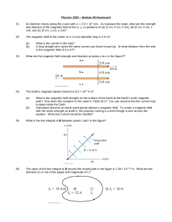
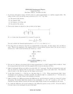
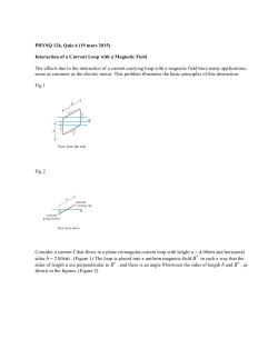
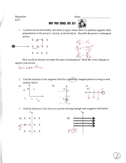
Solar Physics
DOI: 10.1007/•••••-•••-•••-••••-•
A numerical model of MHD waves in a 3D twisted
solar flux-tube
K. Murawski1 · A. Solov’ev2 ·
J. Kra´
skiewicz1
c Springer ••••
Abstract We generalize our analytical and numerical models of the solar fluxtube on twisted magnetic field lines. The basic equations and numerical methods
have much in common with those of Murawski et al. (2015); the new and important issue is the twisted magnetic field component that couples explored torsional
Alfv´en and magnetoacoustic waves. In these models we specify a magnetic flux
function and derive general analytical formulas for the equilibrium mass density
and a gas pressure. We use the developed models, which can be adopted for any
axi-symmetric structure with twisted and untwisted magnetic lines, to simulate
the MHD waves. These waves are excited by a localized pulse in the azimuthal
component of velocity, that is launched at the top of the solar photosphere.
Their propagation through the solar chromosphere and transition region to the
solar corona reveal a complex scenario of twisted magnetic field lines and flows
associated with torsional Alfv´en and magnetoacoustic waves.
Keywords: Waves, Magnetic fields, Corona
1
Group of Astrophysics, UMCS, ul. Radziszewskiego 10,
20-031 Lublin, Poland. email:
[email protected],[email protected]
2
Central (Pulkovo) Astronomical Observatory,
Russian Academy of Sciences, St. Petersburg, Russia. email:
[email protected]
SOLA: flux-tube-Omega_ver6d.tex; 24 March 2015; 10:02; p. 1
K. Murawski et al.
1. Introduction
As a result of the complexity of magnetic field lines and a strongly stratified
solar atmosphere, modeling a realistic magnetic flux-tube in the solar atmosphere consists a formidable task. Despite this complexity and gravitational
stratification, several models of a flux-tube were developed in the past. For
instance, Low (1980) and Gent et al. (2013) (see also the references therein)
constructed flux-tube models in the gravitationally stratified solar atmosphere.
In particular, Low (1980) developed the analytical sunspot model, while Gent
et al. (2013) solved analytically magnetohydrostatic equilibrium within a realistic
atmosphere. Choudhuri (2003) proposed that a twist generation mechanism on
a magnetic flux-tube may originate at the base of the solar convection zone,
the idea of which was later supported by Hotta and Yokoyama (2012) in their
two-dimensional numerical simulations. Zaqarashvili et al. (2014) suggested that
the twisted magnetic flux-tubes can be detected in the solar wind as the variation of total (thermal plus magnetic) pressure. Copil et al. (2010) proved that
the trapped Alfv´en modes exist in a magnetic flux-tube with twisted magnetic
field and straight field in the ambient medium, and these modes are localized
in thin current threads where the magnetic field is twisted. Zhelyazkov and
Zaqarashvili (2012) showed that fast magnetoacoustic kink waves propagating
along photospheric uniformly twisted flux-tubes with axial mass flows experience
the Kelvin-Helmholtz instability under the observed mass flows. A magnetically
twisted compressible flux-tube embedded in a compressible magnetic environment was investigated by Erd´elyi and Fedun (2010) who generalized previous
classical and widely applied studies of magnetohydrodynamic (MHD) waves and
oscillations in magnetic loops without a magnetic twist. See also Erd´elyi and
Fedun (2006, 2007) and Carter and Erd´elyi (2008).
Concerning the name of the torsional transverse MHD wave, in a spatially
bounded magnetic structure like a flux-tube, it can be called either as Alfv´enic
or surface Alfv´en - Alfv´en is the wave that propagates in an infinite magnetized
plasma - the solar corona is, indeed, not such a medium. For the debate about
the name of this wave, see the arguments of Van Doorsselaere et al. (2008) and
SOLA: flux-tube-Omega_ver6d.tex; 24 March 2015; 10:02; p. 2
Twisted flux-tube
the contra-arguments of Goossens et al. (2012). However, throughout this paper
we use the classical term of torsional Alfv´en waves.
Recently, Murawski et al. (2015) devised the analytical and numerical models
of an untwisted solar flux-tube and performed numerical simulation of torsional
Alfv´en waves which decouple from magnetoacoustic waves. These models exhibit
high level of sophistication and complexity of a solar flux-tube. However, the
realistic flux-tubes reveal twisted magnetic field lines, which have to be taken
into account in constructed models.
The aim of this paper is to devise new analytical and numerical models which
exhibit high level of generality and can be adopted to any axi-symmetric magnetic structure with twisted and untwisted magnetic lines. As an application of
these models we perform numerical simulations of torsional Alfv´en waves which
couple to magnetoacoustic waves in the twisted flux-tube.
Our paper is organized as follows. A three-dimensional (3D) model of twisted
magnetic flux-tube embedded in the solar atmosphere is described in Sect. 2.
The numerical model and its application are given in Sect. 3. Conclusions are
presented in the last section.
2. Analytical model of a twisted solar flux-tube
In this part of the paper we consider gravitationally-stratified and magnetized
solar atmosphere that is described by the following ideal, adiabatic, 3D magnetohydrodynamic (MHD) equations:
∂t % + ∇ · (%V) = 0 ,
1
%∂t V + % (V · ∇) V = −∇p + (∇ × B) × B + %g ,
µ
∂t B = ∇ × (V × B) ,
(1)
∇ · B = 0,
kB
%T ,
p=
m
(4)
∂t p + ∇ · (pV) = (1 − γ)p∇ · V ,
(2)
(3)
(5)
where % is mass density, V = (Vx , Vy , Vz ) the fluid velocity, B = (Bx , By , Bz ) the
magnetic field, p gas pressure, T temperature, γ = 5/3 the adiabatic index, µ
SOLA: flux-tube-Omega_ver6d.tex; 24 March 2015; 10:02; p. 3
K. Murawski et al.
magnetic permeability, g = (0, −g, 0) gravitational acceleration with its magnitude g = 274 m s−2 , m mean particle mass that is specified by mean molecular
weight of 1.24, and kB the Boltzmann’s constant.
We adopted ∂t ≡ ∂/∂t notation for temporal partial derivative. Similar
notation will be used for spatial derivatives.
2.1. Equilibrium configuration
We assume that the solar atmosphere is in static equilibrium (V = 0). Then,
from Eqs. (1)–(5), it follows that at this equilibrium a Lorentz-force must be
balanced by the gas pressure gradient and the gravity force, that is
1
(∇ × B) × B = ∇p − %g .
µ
(6)
To satisfy the solenoidal condition of Eq. (4) we introduce the normalized (by
2π) magnetic flux, Ψ, such as
Z
r
Ψ(r, y) =
By r0 dr0 ,
(7)
0
where By is a vertical magnetic field component and r is the radial distance from
the flux-tube axis,
r=
p
x2 + z 2 .
(8)
With the use of Ψ we express the radial, Br , azimuthal, Bθ , and vertical, By ,
components as
1
Br = − ∂y Ψ ,
r
Bθ =
Ω(Ψ)
,
r
By =
1
∂r Ψ ,
r
(9)
where Ω(Ψ) is an arbitrary function which corresponds to a twist in magnetic
field lines.
The magnetic field can also be expressed with the use of the magnetic flux
function, A, such as
B = ∇ × A.
(10)
SOLA: flux-tube-Omega_ver6d.tex; 24 March 2015; 10:02; p. 4
Twisted flux-tube
In Cartesian coordinates without any loose of generality we have
z
x
A = (Ax , Ay , Az ) = A , 0, −A
.
r
r
(11)
With the use of these formulas the solenoidal condition of Eq. (4) is satisfied to
machine errors. Then, adopting Eq. (11) in Eq. (10), we can express magnetic
field components as
Br = ∂y A ,
Bθ =
Ω(Ψ)
,
r
By =
1
∂r (rA) .
r
(12)
Comparing Eqs. (9) and (12), we find
1
Ψ(r, y) .
r
(13)
B · (∇p − %g) = 0 .
(14)
A(r, y) =
From Eq. (6) we get
As p = p(Ψ, y), with the use of Eq. (9) we find that the hydrostatic condition is
fulfilled along magnetic field lines which are specified by Ψ = const, i.e.
%g = −∂y p(Ψ, y) .
(15)
Taking Eq. (9) into account in Eq. (6), we obtain the Grad–Shafranov-type
equation (e.g., Low, 1975; Priest, 2014), i.e.
1
∂r ∂r Ψ − ∂r Ψ + ∂y ∂y Ψ = −µr2 ∂Ψ p(Ψ, y) .
r
(16)
Following Low (1980), we specify a magnetic field through a choice of Ψ,
integrate Eq. (16), and derive the corresponding expressions for p and % in terms
of Ψ and its derivatives. In this approach, we regard y as a parameter, and after
integrating Eq. (16) over Ψ, we find (Solov’ev, 2010)
−
1
µ
2
2
Ω (Ψ) + (∂r Ψ)
+
2r2
Z
r
∞
2
Ω (Ψ)dr
+
r3
where
Z
y
ph (y) = p0 exp −
yr
Z
r
∞
0
dy
Λ(y 0 )
p(r, y) = ph (y)
!
(∂y2 Ψ)∂r Ψ
dr ,
r2
(17)
!
,
(18)
SOLA: flux-tube-Omega_ver6d.tex; 24 March 2015; 10:02; p. 5
K. Murawski et al.
Figure 1. Hydrostatic equilibrium profile of solar temperature for the active Sun
(Avrett & Loeser, 2008).
is the hydrostatic gas pressure (Murawski et al., 2013),
Λ(y) =
kB Th (y)
mg
(19)
is the pressure scale-height and Th (y) is a hydrostatic temperature profile. We
adopt Th (y) for the active solar region that is specified by the atmospheric model
of Avrett & Loeser (2008). This temperature profile is smoothly extended into
the corona (Fig. 1). Then with the use of Eq. (18), we obtain the corresponding
hydrostatic gas pressure profile. Note that the solar photosphere occupies the
region 0 Mm < y < 0.5 Mm, the chromosphere is sandwiched between y = 0.5
Mm and the transition region that is located at y ' 2.1 Mm and is bounded
from above by the solar corona.
With the use of Eq. (15) we determine the equilibrium mass density. From
Eq. (17) we get p = p(r, y). In order to find ∂y p(y, Ψ) we consider the following
relations which are valid for any differentiable function S:
∂r S(r, y) = (∂Ψ S(Ψ, y)) ∂r Ψ ,
(20)
∂y S(r, y) = ∂y S(Ψ, y) + (∂Ψ S(Ψ, y)) ∂y Ψ .
(21)
From Eq. (17) it follows that we need to specify S(r, y) as
Z r 2
Z r 2
(∂y Ψ)∂r Ψ
Ω2 (Ψ) + (∂r Ψ)2
Ω (Ψ)dr
+
+
dr .
S(r, y) =
2
3
2r
r
r2
∞
∞
(22)
SOLA: flux-tube-Omega_ver6d.tex; 24 March 2015; 10:02; p. 6
Twisted flux-tube
We calculate first ∂r S(r, y) and then from Eq. (20) we find ∂Ψ S(y, Ψ). As a
result, we obtain
∂Ψ p(y, Ψ) = −
1 ∂y Ψ
∂r Ψ
1
∂r
+ 2 ∂y2 Ψ .
µ
r
r
r
(23)
Using Eq. (21), we get
∂y p(y, Ψ) = ∂y p(r, y) − (∂Ψ p(y, Ψ)) ∂y Ψ .
(24)
With the use of the above expressions from Eq. (15) we find the equilibrium
mass density, i.e.
(
"
(∂r Ψ) − (∂y Ψ)
1
∂y
+
µg
2r2
2
2
Z
r
∞
%(r, y) = %h (y) +
#
Z r 2
(∂y Ψ)∂r Ψ
Ω (Ψ)dr
+
dr
r3
r2
∞
)
∂y Ψ
∂r Ψ
−
∂r
,
r
r
2
(25)
where
%h (y) =
ph (y)
gΛ(y)
(26)
is the hydrostatic mass density (Murawski et al., 2013).
2.2. A twisted flux-tube
For a twisted flux-tube we can specify A and Ω as
r
1
+ By0 r ,
1 + kr2 r2
2
1
Ω(Ψ) = kΩ rA(r, y)
,
1 + br2 A2 (r, y)
A(r, y) = B0 exp (−ky2 y 2 )
(27)
(28)
where b is a factor, kr , kΩ and ky are inverse length scales along the radial,
azimuthal and vertical directions, respectively. To have a realistic magnetic field
in the solar corona we supplemented the internal magnetic field by the ambient
magnetic field along the vertical direction, By0 . We choose the magnitude of the
reference magnetic field B0 in such way that the magnetic field within the fluxtube, at (x = 0, y = 0, z = 0) Mm, is about 1140 Gauss, and By0 ≈ 11.4 Gauss.
SOLA: flux-tube-Omega_ver6d.tex; 24 March 2015; 10:02; p. 7
K. Murawski et al.
Figure 2. Equilibrium magnetic field lines for the twisted flux-tube: side-view (left)
and top-view (right). Red, green, and blue arrows correspond to the x-, y-, and z-axis,
respectively.
Figure 3. Equilibrium profile of the magnitude of B across the flux-tube at the altitude
y = 0.5 Mm.
The resulting magnetic field lines are displayed in Fig. 2 for b = 0, kr = 5 Mm−1 ,
ky = 2 Mm−1 and kΩ = 0.125 Mm−1 . For these settings, the magnetic field
lines are predominantly vertical around the line, x = z = 0 Mm, while further
out they are bent and become slightly twisted. The magnitude of B at (x =
0, y = 0.5, z = 0) Mm is about 420 Gauss and it falls off with distance from the
vertical line (Fig. 3), reaching a value of By0 at r → ∞ in the ambient medium.
Note that the magnetic field at the top of the simulation region is essentially
SOLA: flux-tube-Omega_ver6d.tex; 24 March 2015; 10:02; p. 8
Twisted flux-tube
Figure 4. Equilibrium profiles of the Alfv´
en (left-solid) and sound (left-dashed) speeds
and plasma β (right) along the flux-tube axis, x = z = 0 Mm.
uniform, with its value close to By0 (Fig. 2), and magnetic field lines have
the helical pitch which falls off with height. This fast fall off results
from the chosen value of ky = 2 Mm−1 . However, the other choices of
ky resulted in negative, and therefore physically unacceptable, values
of the equilibrium mass density.
If one assumes a twisted magnetic flux tube, the torsional Alfv´
en
waves must be coupled with fast and slow magnetoacoustic waves.
Pure torsional Alfv´
en waves can propagate only in an untwisted tube.
The ambient medium is specified by the hydrostatic conditions
which are determined by the temperature profile. Although there is no
clear interface between the ambient medium and the internal tube’s
plasma, we can estimate that at the level of y = 0.5 Mm the tube
radius is about 0.2 Mm and it fast grows with height, reaching a value
of about 1 Mm at y = 2 Mm. As a result of this smoothed interface, the
pressure balance equation was not directly adopted in the construction
of the flux-tube. Instead, it was implicitly implemented in the derived
expression for the equilibrium gas pressure and mass density (Eqs. 17,
25).
Figure 4 illustrates the sound speed, cs (r = 0, y), (left-dashed), Alfv´en speed,
cA (r = 0, y), (left-solid), and plasma β(r = 0, y) (right), where:
c2s (r, y) =
γp(r, y)
,
%(r, y)
c2A (r, y) =
B 2 (r, y)
,
µ%(r, y)
(29)
SOLA: flux-tube-Omega_ver6d.tex; 24 March 2015; 10:02; p. 9
K. Murawski et al.
Figure 5. Numerical blocks with their boundaries (solid lines) and the pulse in velocity
Vz of Eq. (31) (color maps) in the x − y-plane for z = 0 Mm at t = 0 seconds. The low
part of the simulation region is only displayed.
β(r, y) =
2µp(r, y)
.
B 2 (r, y)
(30)
The sound speed below the transition region is about 8 km s−1 , exhibiting a
shallow depression at y ≈ 0.4 Mm. At the transition region cs abruptly raises up
to the coronal value of cs ≈ 80 km s−1 at the level y = 4 Mm. The Alfv´en speed
reveals similar trends, reaching a value of about 250 km s−1 at y = 4 Mm. The
plasma beta is about 0.03 (the right panel) in the solar corona, at y = 4 Mm. It
raises with depth, staying larger than 1 for y < 1.7 Mm.
SOLA: flux-tube-Omega_ver6d.tex; 24 March 2015; 10:02; p. 10
Twisted flux-tube
3. Numerical model of MHD waves in the twisted flux-tube
We implement the expression for the equilibrium mass density, gas pressure, and
the magnetic field which result from the analytical model described in Sect. 2
into the code FLASH (Lee & Deane, 2009; Lee, 2013). This code solves the
initial-value problem for Eqs. (1)–(5), adopting the staggered mesh scheme in a
fashion of a finite-volume, Godunov-type method which consists of constrained
transport to fulfill the solenoidal constraint. This code implements a third-order
unsplit Godunov solver (e.g. Murawski & Lee, 2011) with various slope limiters
and Riemann solvers, as well as adaptive mesh refinement. We choose the van
Leer slope limiter and the Roe Riemann solver (e.g. Murawski & Lee, 2012).
For all considered cases, we set the simulation box as (−1, 1) Mm ×(0, 14)
Mm ×(−1, 1) Mm and impose boundary conditions by fixing in time all plasma
quantities at all six boundary surfaces to their equilibrium values. In the present
numerical studies, we use a non-uniform grid with a minimum (maximum) level
of refinement set to 2 (5). The grid system at t = 0 s is shown in the vertical
plane for z = 0 Mm in Fig. 5. Note that the blocks are displayed only up to
y = 6 Mm. Above this altitude the block system is uniform. As there are 8×8×8
identical grid cells in every numerical block, we reach the effective finest spatial
resolution of 15.625 km, below the altitude, y = 2.5 Mm.
We adopt the developed numerical model of a twisted flux-tube for MHD
waves which are excited in the system by launching the initial pulse in azimuthal
component of velocity, i.e.
2
x + z 2 + (y − y0 )2
z −x
ˆ
,
AV exp −
,
Vθ θ = (Vx , Vz ) =
w w
w2
(31)
where AV denotes the amplitude of the pulse, θˆ is the unit vector along the
azimuthal direction, y0 its vertical position, and w its width. We set AV = 6
km s−1 , w = 150 km, and y0 = 500 km, and hold them fixed. This value of AV
results in effective maximum velocity of about 2.2 km s−1 (Fig. 5).
In a twisted flux-tube, the initial velocity pulse of Eq. (31) triggers torsional
Alfv´en and magnetoacoustic-gravity waves. Torsional Alfv´en waves were the
subject of theoretical studies by Hollweg (1981) and Hollweg et al. (1982) who
SOLA: flux-tube-Omega_ver6d.tex; 24 March 2015; 10:02; p. 11
K. Murawski et al.
analyzed linear propagation of twists. The authors concluded that the waves
are able to heat the solar corona. Recently, Murawski et al. (2015) studied
these waves in the framework of the newly constructed model of an untwisted
flux-tube. They inferred that Alfv´en waves, which in this case decouple from
magnetoacoustic waves, are able to affectively drive slow magnetoacoustic waves
by ponderomotive force. In the twisted flux-tube the torsional Alfv´en and magnetoacoustic waves are coupled and therefore they suppose to alter dynamics of
plasma.
Figure 6 shows magnetic field lines at four moments of time. At t = 100 s (the
top-left panel) the upwardly propagating Alfv´en waves reach the altitude y ≈ 1
Mm, and at a later time Alfv´en waves spread in space while propagating along
diverged with y magnetic field lines (the top-right and bottom panels). Note that
perturbations of magnetic field lines remain weak in the solar corona. This is also
clearly evident in the spatial profiles of Bz (x, y, z = 0) as displayed at t = 200 s
and t = 250 s (Fig. 7, the bottom panels). At t = 100 s, t = 150 s (the top panels),
and t = 200 s (bottom-left), the perturbations of Bz (x, y, z = 0) are localized
below the transition region but at later times the perturbations that penetrate
the inner solar corona are of lower magnitude than those remaining below the
transition region. Consequently, these profiles demonstrate clearly that Alfv´en
waves, while traced in perturbed magnetic field lines, are essentially located
below the transition region, which agrees with the conclusions of Murawski &
Musielak (2010) who used the analytical and numerical techniques for the 1D
wave equations and found that magnetic field perturbations, while excited below
the transition region, remain week in the solar corona in comparison to the
perturbations in lower atmospheric layers. Similar conclusions were drawn by
Murawski et al. (2015) who studied torsional Alfv´en waves within the framework
of an untwisted flux-tube model.
Figure 8 shows temporal snapshots of velocity streamlines at few moments of
time. These streamlines are defined by the following equations:
dy
dz
dx
=
=
.
Vx
Vy
Vz
(32)
SOLA: flux-tube-Omega_ver6d.tex; 24 March 2015; 10:02; p. 12
Twisted flux-tube
Figure 6. Magnetic field lines at t = 100 s (top-left), t = 150 s (top-right), t = 200
s (bottom-left), and t = 250 s (bottom-right). Red, green and blue arrows design the
directions of the x-, y-, and z-axis, respectively.
SOLA: flux-tube-Omega_ver6d.tex; 24 March 2015; 10:02; p. 13
K. Murawski et al.
Figure 7. Spatial profiles of Bz (x, y, z = 0) associated with torsional Alfv´
en waves,
at t = 100 s (top-left), t = 150 s (top-right), t = 200 s (bottom-left), and t = 250 s
(bottom-right).
SOLA: flux-tube-Omega_ver6d.tex; 24 March 2015; 10:02; p. 14
Twisted flux-tube
Figure 8. Streamlines at t = 100 s (top-left), t = 150 s (top-right), t = 200 s
(bottom-left), and t = 250 s (bottom-right). Red, green and blue arrows design the
directions of the x-, y-, and z-axis, respectively.
Note that a signal in the azimuthal velocity is clearly seen in the solar corona
at t = 250 s (Fig. 8, bottom-right). Indeed, the streamlines show that velocity
perturbations penetrate the transition region and enter the solar corona, leading
to a generation of the main centrally located vortex, which starts developing at
t = 200 s (bottom-left).
SOLA: flux-tube-Omega_ver6d.tex; 24 March 2015; 10:02; p. 15
K. Murawski et al.
Figure 9. Spatial profiles of Vz (x, y, z = 0) associated with torsional Alfv´
en waves at
t = 100 s (the top-left panel), t = 150 s (the top-right panel), t = 200 s (the bottom-left
panel), and t = 250 s (the bottom-right panel).
SOLA: flux-tube-Omega_ver6d.tex; 24 March 2015; 10:02; p. 16
Twisted flux-tube
Torsional Alfv´en waves can also be traced in the vertical profiles of Vz (x, y, z =
0) = Vθ (x, y, z = 0) (see Fig. 9). The downwardly propagating waves subside
as they already left the simulation box at t ≈ 200 s (the bottom-left panel),
propagating away through the bottom boundary. At t = 250 s (the bottom-right
panel), the upwardly propagating Alfv´en waves resulting from the initial pulse
are well seen, with their amplitudes of |Vz | ≈ 5.7 km s−1 . The reflected from
the transition region torsional Alfv´en waves are discernible in the bottom-right
panel as a propagating downwards wave-front.
4. Discussion and conclusions
In this paper, we present a new analytical model of a 3D twisted magnetic
flux-tube embedded in the solar atmosphere whose photospheric, chromospheric
and transition region’s temperatures are described by the model of Avrett &
Loeser (2008). The model was used to perform numerical simulations of the
propagation of torsional Alfv´en and magnetoacoustic-gravity waves by using the
FLASH code. These torsional Alfv´en waves are launched at the top of the solar
photosphere by an initial localized pulse in the azimuthal component of velocity.
Our numerical results show that the excited perturbations in azimuthal component of the magnetic field (Fig. 7) are seen below the solar transition region,
however, in the inner corona these perturbations are of a significantly lower amplitude. On the other hand, the perturbations in azimuthal component of velocity
are stronger in the solar corona, and the scenario of MHD waves propagation is
similar to that in the untwisted flux-tube (Murawski et al. 2015).
We conclude that our analytical model can easily be adopted to derive the
equilibrium conditions for any 3D axi-symmetric structure with twisted and
untwisted magnetic lines, which are specified by a magnetic flux function and a
twist. The latter can be set to zero to an untwisted flux-tube. Our newly-devised
numerical model of the 3D solar magnetic flux-tube can be applicable to the
variety of flux-tubes with different photospheric fields, and different expansions,
as well as with different strengths of the drivers. The only constraint in this
model are positive values of mass density and gas pressure.
SOLA: flux-tube-Omega_ver6d.tex; 24 March 2015; 10:02; p. 17
K. Murawski et al.
Acknowledgements
The authors express their thanks to the referee for his/her stimulating
comment. This work has been supported by a Marie Curie International Research Staff Exchange Scheme Fellowship within the 7th European Community Framework Program (KM).
The software used in this work was in part developed by the DOE-supported ASC/Alliance
Center for Astrophysical Thermonuclear Flashes at the University of Chicago.
References
Avrett, E.H., Loeser, R.: 2008, ApJS, 175, 228.
Carter, B.K., Erd´
elyi, R.: 2008, A&A, 481, 239.
Choudhuri, A.: 2003, Sol. Phys., 215, 31.
Copil, P., Voitenko, Y., Goossens, M.: 2010, A&A, 510, A17.
Erd´
elyi, R., Fedun, V.: 2006, Solar Phys., 238, 41.
Erd´
elyi, R., Fedun, V.: 2007, Solar Phys., 246, 101.
Erd´
elyi, R., Fedun, V.: 2010, Solar Phys., 263, 63.
Gent, F.A., Fedun, V., Mumford, S.J., Erd´
elyi, R.: 2013, MNRAS, 435, 689.
Goossens, M., Andries, J., Soler, R., Van Doorsselaere, T., Arregui, I., Terradas, J.: 2012, ApJ,
753, 111.
Hollweg, J.V.: 1981, Sol. Phys., 70, 25.
Hollweg, J.V., Jackson, S., Galloway, D.: 1982, Solar Phys., 75, 35.
Hotta, H., Yokoyama, T.: 2012, A&A, 548, 74.
Lee, D.: 2013, J. Comput. Phys., 243, 269.
Lee, D., Deane, A.E.: 2009, J. Comput. Phys., 228, 952.
Low, B.C.: 1975, ApJ, 197, 251.
Low, B.C.: 1980, Solar Phys., 67, 57.
Murawski, K., Musielak, Z.E.: 2010, A&A, 518, A37.
Murawski, K, Lee, D.: 2011, Bull. Pol. Ac.: Tech., 59, 81.
Murawski, K, Lee, D.: 2012, Control and Cybernetics, 42, 35.
Murawski, K., Ballai, I., Srivastava, A.K., Lee, D.: 2013, MNRAS, 436, 1268.
Murawski, K., Srivastava, A.K., Musielak, Z.E.: 2014, ApJ, 788, 1.
Murawski, K., Solov’ev, A., Musielak, Z., Srivastava, A.K., Kra´skiewicz, J.: 2015, A&A,
submitted.
Priest, E.R.: 2014, Magnetohydrodynamics of the Sun, Cambridge University Press, New York.
Solov’ev, A.A.: 2010, Astronomy Reports, 54, 85.
Van Doorsselaere, T., Nakariakov, V.M., Verwichte, E.: 2008, ApJ, 676, L73.
Zaqarashvili, T., V¨
or¨
os, Z., Narita, Y., Bruno, R.: 2014, ApJ, 783, L19.
Zhelyazkov, I., Zaqarashvili, T.V.: 2012, A&A, 547, 14.
SOLA: flux-tube-Omega_ver6d.tex; 24 March 2015; 10:02; p. 18