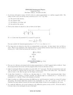
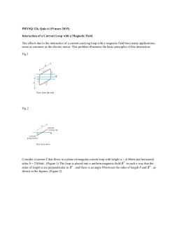
Jonah Shaver,†,储,p A. Nicholas G. Parra-Vasquez,‡,储 Stefan Hansel,§,⬜ Oliver Portugall,⬜ Charles H. Mielke,¶
Michael von Ortenberg,§ Robert H. Hauge,# Matteo Pasquali,‡ and Junichiro Kono†,*
†
Department of Electrical and Computer Engineering, Rice University, Houston, Texas 77005, ‡Department of Chemical and Biomolecular Engineering, Rice University,
Houston, Texas 77005, §Institut für Physik, Humboldt-Universität zu Berlin, Berlin, Germany, ⬜Laboratoire National des Champs Magnétiques Pulsés, 31400 Toulouse,
France, ¶National High Magnetic Field Laboratory, Los Alamos, New Mexico 87545, and #Department of Chemistry, Rice University, Houston, Texas 77005. 储Jonah Shaver
and A. Nicholas G. Parra-Vasquez contributed equally to this work. pCurrent address: Centre de Physique Mole´culaire Optique et Hertzienne, Universite´ de Bordeaux
and CNRS, 351 cours de la Libe´ration, Talence, F-33405, France.
S
ingle-walled carbon nanotubes
(SWNTs), rolled up tubes of graphene
sheets, are unique nano-objects with
extreme aspect ratios, which lead to unusually anisotropic electrical, magnetic, and optical properties. They can be individually
suspended in aqueous solutions with appropriate surfactants,1 and such suspended
SWNTs behave roughly as rigid rods undergoing Brownian motion.2 In the absence of
external fields, their orientation angles are
randomly distributed. However, when
placed in a perturbing field, suspended
SWNTs will align parallel to the field lines
owing to their anisotropic properties. The
steady state alignment of SWNTs in
magnetic,3⫺7 electric,9 flow,10⫺14 and strain
fields15 has been characterized in many recent studies. Though mentions of dynamic
alignment have been made,16,17 to date
there are no comprehensive studies. Here
we present the first combined experimental and theoretical study that provides fundamental insight into the hydrodynamic
motion of these highly anisotropic nanoobjects.
The magnetic susceptibilities of SWNTs
of different diameters, chiralities, and types
have been theoretically calculated using different methods.18⫺21 Semiconducting
SWNTs are predicted to be diamagnetic (␹
⬍ 0) both parallel (储) and perpendicular (⬜)
to their long axis, but the perpendicular susceptibility is predicted to have a larger magnitude (|␹⬜| ⬎ |␹储|), aligning the SWNT parallel to the field. Metallic SWNTs are
predicted to be paramagnetic (diamagnetic) parallel (perpendicular) to their long
www.acsnano.org
ARTICLE
Alignment Dynamics of Single-Walled
Carbon Nanotubes in Pulsed Ultrahigh
Magnetic Fields
ABSTRACT We have measured the dynamic alignment properties of single-walled carbon nanotube (SWNT)
suspensions in pulsed high magnetic fields through linear dichroism spectroscopy. Millisecond-duration pulsed
high magnetic fields up to 56 T as well as microsecond-duration pulsed ultrahigh magnetic fields up to 166 T were
used. Because of their anisotropic magnetic properties, SWNTs align in an applied magnetic field, and because of
their anisotropic optical properties, aligned SWNTs show linear dichroism. The characteristics of their overall
alignment depend on several factors, including the viscosity and temperature of the suspending solvent, the
degree of anisotropy of nanotube magnetic susceptibilities, the nanotube length distribution, the degree of
nanotube bundling, and the strength and duration of the applied magnetic field. To explain our data, we have
developed a theoretical model based on the Smoluchowski equation for rigid rods that accurately reproduces the
salient features of the experimental data.
KEYWORDS: carbon nanotubes · optical properties of carbon nanotubes · dichroism
of molecules · absorption spectra of molecules · light absorption and transmission ·
generation of high magnetic fields
axes (␹储 ⬎ 0, ␹⬜ ⬍ 0) and thus also align
parallel to the applied field. For ⬃1-nmdiameter nanotubes, the values for the
magnetic anisotropy, ⌬␹ ⫽ ␹⬜ ⫺ ␹储, calculated by an ab initio method are between
1.2 and 1.8 ⫻ 10⫺5 emu/mol, depending on
the tube chirality,21 which are similar to
the values calculated by a k · p method (1.9
⫻ 10⫺5 emu/mol)20 and by a tight-binding
method (1.5 ⫻ 10⫺5 emu/mol).19 These values are consistent with recently reported
experimental values, measured with steadystate optical methods.5,8
The degree of alignment of SWNTs in a
magnetic field can be conveniently characterized by the dimensionless ratio of the
alignment potential energy and the thermal energy,
ξ)
*Address correspondence to
[email protected].
Received for review August 15, 2008
and accepted November 24, 2008.
Published online December 22, 2008.
10.1021/nn800519n CCC: $40.75
2
B N∆χ
kBT
(1)
© 2009 American Chemical Society
VOL. 3 ▪ NO. 1 ▪ 131–138 ▪ 2009
131
ARTICLE
where B is the magnetic field, N is the number of carbon atoms in the SWNT, kB is the Boltzmann constant,
and T is the temperature of the solution. A significant
fraction of nanotubes in the solution will align with B
when the alignment energy is greater than the randomizing energy, that is, when ␰ ⬎ 1. Using u and the angle
(␪) between a SWNT and the aligning magnetic field,
an angular distribution function,22 P(␪), in thermal equilibrium can be calculated as23
dP(θ)
)
dθ
exp(ξ2 cos2 θ) sin θ
∫
π⁄2
0
(2)
exp(ξ2 cos2 θ) sin θ dθ
Many experiments have studied the equilibrium alignment of SWNTs in magnetic fields. 3,6,22,24 More recent
experiments have explored the chirality dependence of
SWNT alignment to extract the SWNT species specific
magnetic susceptibilities.8
Linear dichroism spectroscopy has a well-developed
history of application to both steady state and dynamic
situations, such as the flow-induced alignment of
fibrils25 and the magnetic-field-induced alignment of
polyethylene and carbon fibers.26 However, to date no
one has studied the dynamic effects of alignment of
SWNTs. Defined as the difference between the absorbance of light polarized parallel (A储) and perpendicular
(A⬜) to the orientational director of a system, nˆ, linear
dichroism (LD) is a measure of the degree of alignment
of any solution of anisotropic molecules.27 Experimentally, the sign of LD gives qualitative information about
the relative orientation of molecules, positive for alignment parallel to nˆ and negative for perpendicular. Reduced LD, LDr, is normalized by the unpolarized, isotropic absorbance (A) of the system, and gives a
quantitative measure of the alignment. The measured
LDr spectrum is related to both the polarization of the
transition moment being probed and the overall degree of alignment of the molecules being investigated:27
LDr )
(
)
3 cos2 R - 1
LD A| - A⊥
)
)3
S
A
A
2
(3)
where ␣ is the angle between the transition moment
and the long axis of the molecule and S is the nematic
order parameter. S is a dimensionless quantity that
scales from 0 for an isotropic sample to 1 for a perfectly aligned sample and is defined as
S)
3〈cos2 θ〉 - 1
2
(4)
where 具cos2 ␪典 is averaged over the angular probability distribution function and ␪ is the microscopic angle
made between a SWNT’s long axis and the alignment
director of the system.
132
VOL. 3 ▪ NO. 1 ▪ SHAVER ET AL.
For the case of SWNTs, optical selection rules28
coupled with a strong depolarization for light polarized perpendicular to the tube axis result in appreciable
absorption features observed only when light is polarized parallel to the tube axis. Hence, we can simplify eq
3 using ␣ ⫽ 0, to LDr ⫽ 3S, giving a direct link between the measured LDr and the orientation of the
SWNTs.
In this study, the dynamic effects of SWNT alignment in pulsed high magnetic fields were investigated
for the first time. We measured time-dependent transmittance through individually suspended SWNTs in
aqueous solutions in the Voigt geometry (light propagation perpendicular to the applied magnetic field) in
two polarization configurations, parallel and perpendicular to the applied magnetic field. From this we calculated LD as a function of time, both in millisecond
(ms)-long pulsed high magnetic fields up to 56 T and
microsecond (␮s)-long pulsed ultrahigh magnetic fields
up to 166 T. We developed a theoretical model based
on the Smoluchowski equation, which extracts the
length distribution of the SWNTs in suspension based
on a fit to time-dependent LD. These results pave the
way to further study of SWNT dynamics in solution.
RESULTS
Measured Transmittance. All ms-pulse data was taken
using a spectrally resolved, near-infrared setup. To
avoid any convolution with spectral line shape broadening and splitting4,5,16 the data was integrated over
the entire InGaAs range (⬃900 to 1800 nm). The benefit of removing ambiguity associated with spectral
changes induced by the Aharonov⫺Bohm29 effect
coupled with the large number of nanotube chiralities
present in our sample outweighs the possibility for any
chirality selective analysis (which has been performed
at low magnetic fields8).
Figure 1a displays spectrally integrated, timedependent transmittance through the sample and polarizer [in parallel (blue) and perpendicular (red) configurations] and the accompanying 56 T magnetic field
trace (green). The raw transmittance data is normalized
to the zero-field value as
N
T|,⊥
(t) )
T|,⊥(t)
T(t ) 0)
(5)
where T储, ⬜(t) denotes the raw transmittance as a function of time with the respective polarization configuration. Starting at time zero, before the field pulse, the
transmittance in both polarization configurations is
equal. As the field increases, and the SWNTs start to
align with the field, light polarized parallel (perpendicular) to the magnetic field decreases (increases) in overall transmittance.
Similarly, Figure 1b shows the optical response of
suspended SWNTs to a ␮s-pulse magnetic field prowww.acsnano.org
ARTICLE
Coil Project (STP) magnet31 in a perpendicular configuration with a 635 nm laser and a different sample. At approximately 6 ␮s, when magnitude of the field was
low, in part c the detector overloaded due to the arc
flash from the routine disintegration of the coil; this
does not affect the data collected before the coil break.
This data confirms our results from the Megagauss Generator with a different magnet of similar design, different excitation wavelength, and different sample. Overall, the magnitude of the change in transmittance is less
than the ms pulse experiment due to the shorter field
duration. Figure 1, panels a and d are nearly the same
magnitude, but the ␮s-pulse in 1d shows an order of
magnitude smaller response than the ms-pulse in 1a.
For our qualitative analysis we use ms-pulse data from
Toulouse and ␮s-pulse data from Berlin.
Calculated Dynamic Linear Dichroism. The time-dependent
(or dynamic) linear dichroism, LD(t), of SWNT alignment
is calculated directly from the normalized transmittances. Using the relationship between transmittance
(T) and absorbance (A), LD(t) can be related to the measured transmittances, T储(t) and T⬜(t), as
LD(t) ) A|(t) - A⊥(t)
) -ln
) ln
Figure 1. (color online) Time-dependent traces of transmittance of light polarized parallel (red, left axis) and perpendicular (blue, left axis) to the applied magnetic field (green,
right axis) for (a) a 56 T, 50-ms-risetime pulse, (b) a 140 T, 2.5␮s-risetime pulse (Megagauss), (c) a 166 T, 2.5-␮s-risetime
pulse (STP) in the perpendicular polarization geometry, and
(d) 65 T oscillating ␮s-field pulse and transmittance in parallel polarization geometry. At zero magnetic field, the transmittances are equal. As the field strength grows, the SWNTs
align and decrease (parallel) or increase (perpendicular) the
intensity of transmitted light.
duced by the Megagauss Generator in Berlin.30 This
data was collected with an Ar⫹ ion laser at 488 nm,
which is in the second sub-band region of the SWNT optical spectra, and thus the Aharonov⫺Bohm effect induced spectral changes are small in relation to the line
width, negating the need for spectral integration. As the
field rises to 140 T (⬃2.5 ␮s risetime), the nanotubes
align to their maximum value, which lags the peak field
by ⬃2 ␮s. It should be noted that in this experiment
the field returns to zero at ⬃6 ␮s and then increases in
the negative direction, reaching a minimum ⬇ ⫺50 T at
⬃9 ␮s. However, since only the magnitude of the magnetic field (|Bជ |) is important in aligning the nanotubes,
the transmittance shows a secondary peak at ⬃10 ␮s.
This is also clearly demonstrated by the parallel configuration data in Figure 1d where we used the Megagauss
Generator to produce a rapidly oscillating field ⬇ 65 T.
Figure 1c shows results from the Los Alamos Single Turn
www.acsnano.org
T⊥(t)
T|(t)
+ ln
T0
T0
T⊥(t)
T|(t)
(6)
where the transmittance of the background medium,
T0, cancels out. This is of particular advantage in pulsed
field experiments, where the induced change in transmittance is very straightforward to collect, but the background signal can be cumbersome. As we are studying
the dynamics of SWNT alignment in pulsed fields, and
not the magnitude of alignment, we can utilize LD(t)
normalized to its maximum value (LD(t) ⬅ LD(t)/LDmax).
Although this procedure washes out the quantitative
measure of the alignment as opposed to normalizing
by isotropic absorption as in LDr ⫽ 3S, it retains the dynamics of the SWNTs in response to the magnetic field
pulse.
Figure 2 shows LD(t) (purple) for (a) ms and (b) ␮s
pulses calculated from the transmittances of Figure 1.
The relationship of LD and LDr is such that they share
the same dynamic features. The positive sign of the signal indicates that the SWNTs are aligning with the magnetic field. As the strength of the magnetic field increases, it reaches a critical value (length dependent)
where the magnetic force overcomes Brownian motion.
At this point, SWNTs start aligning and continue to
align as long as the magnetic field remains above this
critical value. However, the overall alignment of the
SWNTs lags behind the applied field because of viscous drag. As the field decreases, Brownian motion becomes again more significant; beyond a critical field
VOL. 3 ▪ NO. 1 ▪ 131–138 ▪ 2009
133
ARTICLE
Figure 3. A SWNT with a direction defined by the vector u
at an angle ␪ to the magnetic field B; the magnetic properties of the SWNT creates a torque Nmag forcing the SWNT to
align with the magnetic field. Its direction changes as u˙, defining an angular velocity ␻ ⴝ u ⴛ u˙.
which is the sum of contributions from Brownian motion and the magnetic field. If ⌿(L; u; t) is the probability distribution function of u and U(L; u; t) is the external
potential, then the Brownian motion contribution is included by adding kBT ln ⌿ to U. The angular velocity ␻
induced by the total torque is32
1
1
ω ) Ntot ) - (kBTR ln Ψ + RU)
ςr
ςr
Figure 2. (color online) Time-dependent traces of calculated
normalized dynamic linear dichroism LD(t) (purple, left axis)
and applied magnetic field (green, right axis) for (a) a 56 T,
ms-pulse and (b) a 140 T, ␮s-pulse. As the sample is isotropic at zero magnetic field, the linear dichroism is zero. As the
field strength grows in time and the SWNTs align with the
magnetic field, the dichroism increases, peaking at a time
slightly lagged to the maximum of the magnetic field. After
the magnetic field pulse, the sample gradually relaxes to its
unaligned state. Comparison to normalized linear dichroism
computed from our model is shown in solid black.
strength (corresponding to the maximum LD) the
SWNTs begin to progressively lose orientation, slowed
by viscous drag. At the end of the magnetic pulse, the
residual SWNT alignment decays exponentially in time
under the effect of Brownian motion with a characteristic time dictated by ␶r ⫽ 1/(6Dr), where Dr is defined
later in eq 14.
Theory. To understand the effect of the magnetic field
on the overall alignment of the SWNTs in solution, we
must understand the competition between thermal agitation, or Brownian motion, which functions to randomize the nanotube orientation and the magnetic field,
which functions to align the nanotubes. Since the persistence length of a single SWNT is much greater than the
length of the SWNTs in our study,2 we consider SWNTs to
behave like rigid-rods in suspensions of radius R and polydisperse length L. We examine a dilute dispersion of noninteracting SWNTs, which enables us to consider the orientation of each nanotube independently and determine
the bulk orientation by summing the contributions from
each nanotube in the distribution.
Figure 3 depicts a SWNT oriented in the direction u
at an angle ␪ to the magnetic field B; the SWNT orientation is dependent on the total torque,
Ntot ) NBrown + Nmag ,
134
VOL. 3 ▪ NO. 1 ▪ SHAVER ET AL.
(7)
(8)
where the rotational operator ᏾ is defined as
R≡u×
∂
∂u
(9)
and the rotational friction constant ␵r is defined as33
ςr )
πηsL3
εf(ε)
3
(10)
where
-1
( RL )
ε ) ln
(11)
and
f(ε) )
1 + 0.64ε
+ 1.659ε2
1 - 1.5ε
(12)
The equation for the conservation of the probability distribution ⌿ then becomes
[
]
Ψ
∂Ψ
) -R · (ωΨ) ) DrR · RΨ +
RU
∂t
kBT
(13)
where the rotational diffusion is defined as
Dr )
kBT
ςr
(14)
Equation 13 is known as the Smoluchowski equation
for rotational diffusion.32
In our system the external potential is the magnetic
field’s effect on the orientation of an individual SWNT.
This potential depends on the magnetic susceptibility
anisotropy, ⌬␹, of the SWNT, the number of carbon atwww.acsnano.org
[(
U ) ∆χNB2 cos2 θ ) ∆χNB2
4
3
)]
1
κ(Y + ) (17)
3
π 0 1
Y +
)
5 2 3
0
2
where
κ(L;t) )
4
3
π5 ∆χ N(L) B(t)
2
ARTICLE
The energy can be expressed simply in terms of the
second spherical harmonic Y20
(18)
The partial differential equations, eq 13, are then converted into a system of ordinary differential equations
for Anm using Galerkin’s method. By multiplying eq 13 by
each basis function Yqp and integrating over all orientations, the time evolution of each corresponding coefficient, d/dt (Aqp), can be determined as
)
∫ sin θ dθ∫ dφY dΨ
dt
∫ sin θ dθ∫ dφY dtd ∑ ∑
p
q
p
q
AnmYnm )
0eneN -nemen
Figure 4. (color online) The contributions from each length
in the distribution normalized to their maximum value (dotted black), the experimental LD (purple), and the accompanying magnetic field pulses (green). Traces are offset for clarity, and the field and experimental traces are reproduced at
each offset for ease of comparison. Note that no single dotted trace can successfully reproduce the experimental LD: (a)
ms-pulse, (b) ␮s-pulse.
n even
U(L;u;t) ) -∆χN(L) B(t)2 cos2 θ(u)
6κ
Dr
kBT
∑ ∑
0eneN -nemen
Ψ(L;u;t) )
∑ ∑
Anm(L;t)Ynm(u)
(16)
0eneN -nemen
n even
m even
Spherical harmonics are ideal basis functions because
they are eigenfunctions of the highest derivative operator in eq 13. Note that only the even values of n are
used because the system is symmetric about the alignment axis. Note also that only the even values of m are
needed since the SWNTs have no permanent magnetic
moments (they have only induced magnetic dipoles),
and so ⌿(u) ⫽ ⌿(⫺u).34
www.acsnano.org
Dr
κ
kBT
Anm
∫ sin θ dθ∫ dφ Y Y
p m 0
q n Y2 -
m even
∑
∑
n even
m even
2eneN -n+2emen
Anm
32 (n - m)(n + m + 1) ×
∫ sin θ dθ∫ dφ Y Y
p m-1 1
Y2 q n
(15)
To track the nematic order parameter S(t) of the SWNT
suspension in a time-dependent magnetic field, we first
solve the Smoluchowski equation by expanding ⌿ as
a sum of spherical harmonics Ynm:
m even
)-Drq(q + 1)Aqp -
n even
oms in the SWNT, N(L), the strength of the magnetic
field, B(t), and the orientation of the SWNT as measured
by the angle ␪(u):
d p
A (19)
dt q
κ
Dr
kBT
∑
∑
n even
m even
2eneN -nemen-2
Anm
32 (n + m)(n - m + 1) ×
∫ sin θ dθ∫ dφ Y Y
p m+1 -1
Y2
q n
(20)
where the integrals of the multiplication of three spherical harmonics, that is, 兰 sin ␪ d␪ 兰 d␾ Ypq Ynm⫹1, m, m⫺1
Y2⫺1, 0, 1, are nonzero only when m ⫽ p ⫽ 0 or p ⫽ ⫺m.35
The initial values of the coefficients are determined
from the initial orientation of the nanotubes; a random
orientation is described by Anm ⫽ 0 except for A00 ⫽ 1.
The magnetic field is turned on at t ⫽ 0 and varies with
time. The coefficients at each time step are solved by
using a numerical ordinary differential equation integration technique: third-order Runge⫺Kutta, available
in MATLAB (ODE23). S is related with the coefficients,
Anm(L), through 具cos2 ␪典,
VOL. 3 ▪ NO. 1 ▪ 131–138 ▪ 2009
135
ARTICLE
〈cos2 θ〉 )
〈
4
3
(
4
3
〉
π 0 1
Y + )
5 2 3
π 0 1
Y +
5 2 3
)∑
∫ sin θ dθ∫ dφ
∑
0eneN -nemen
n even
4
3
AnmΨnm )
m even
∫ sin θ dθ∫ dφ(Y )
π 0
A
5 2
0 2
2
+
∫ sin θ dθ ∫ dφ ) 34 π5 A + 31 (21)
1 0
A
3 0
0
2
By placing eq 21 into eq 4, we find S(L, t) to be
π5 A (L;t)
0
2
S(L;t) ) 2
(22)
The bulk solution’s nematic order parameter S(t) is determined by integrating S(L; t) over the distribution of
lengths
π5 ∫ A (L, t) Ω(L) dL
S(t) ) 2
∞
0
0
2
(23)
To compare with experimental data, we assume a lognormal probability distribution,
Ω(L) )
(
1
(ln L - µ)2
exp 2σ2
Lσ√2π
)
(24)
and vary the parameters ␮ and ␴, the mean and standard deviation of log L, respectively, to calculate LD(t) ⫽
max (S(t))/S(t), which is compared with our measured
LD(t).
DISCUSSION
We can now use our model to calculate the dynamic response of SWNTs in time-varying magnetic
Figure 5. Colormaps showing alignment as a function of length for
the millisecond pulse (a) and the microsecond pulse (b). The black
graphs on the left and the green graphs above and below are the corresponding fit distributions (log scale) and magnetic fields,
respectively.
136
VOL. 3 ▪ NO. 1 ▪ SHAVER ET AL.
Figure 6. (color online) Magnetic field dependent traces of
calculated (purple) and simulated (black) normalized linear
dichroism vs applied magnetic field. The hysteresis is indicative of the lag to the magnetic field produced by our polydisperse length sample: (a) 56 T, ms-pulse, and (b) 140 T, ␮spulse.
fields and compare with the experimental data. Figure
4 compiles simulated LD for several lengths. Each simulated LD trace (dotted black) is offset vertically and plotted alongside its applied magnetic field (green) and experimental LD (purple). In the Smoluchowski equation,
orientation is controlled by the competition between
magnetic and Brownian torques; however, the overall
dynamics are slowed by the viscous drag. The magnetic
energy varies with L and the viscous drag varies with
L3, that is, shorter tubes do not align as much as longer
ones but reach their equilibrium alignment more
quickly. Thus, in the millisecond magnetic pulse (Figures 4a and 5a) the dynamics are dominated by the
longer tubes as they align more significantly and need
a longer time to relax, while short tubes that align
quickly dominate the signal of the microsecond pulse
(Figures 4b and 5b).
Because we have a sample that is polydisperse in
length, as expected, no individual simulated length is
able to reproduce all the features of the experimental
data, as shown in Figure 4. To describe a typical SWNT
length distribution, we use a log-normal form, which
has been measured and confirmed by AFM and rheology measurements on similarly prepared samples.13 In
Figure 7 the lengths indicated by symbols are those
that were explicitly calculated to determine the overall
LD that best fit our experiment. Figure 6 compares the
experimental LD signal with that obtained from our
simulation as a function of magnetic field. Our model
shows a good overall match to the measured data uswww.acsnano.org
ing published values5 for ⌬␹, the corresponding alignment potential from eq 15, and the length distribution,
⍀(L) from eq 24. These results were obtained by varying average, ␮, and standard deviation, ␴, of the natural log of L in a log-normal distribution (Figures 5⫺7).
The comparisons in Figure 2 are fit by the length distributions of Figure 7. Figure 4 gives an indication of
which population of SWNTs is responsible for each part
of the simulated LD. Shorter nanotubes are the predominant source of signal during the upsweep of the
field and longer nanotubes for the down sweep (and
lag). As the samples were not from the same batch for
the different time duration pulses, a rigorous comparison between these effects cannot be made. Nonetheless, it is feasible to conclude that a shorter duration
CONCLUSION
We have measured the magnetic-field-induced dynamic linear dichroism of SWNT solutions. Our presented technique establishes a method for the extraction of the length distribution of the SWNTs present in
solution based on the Smoluchowski equation. However, future work is needed, specifically comparison
with other techniques for determining length distributions, such as rheology and AFM measurements, allowing for refinement of published values of SWNT magnetic susceptibility and chirality dependence. It is also
possible from this work to design experiments that will
predominantly probe certain lengths of SWNTs in solution, and investigate the possibility of varying length
distributions with chirality.
METHODS
Megagauss Generator and the STP magnet are single-turn
coil magnets of similar design. They each utilize low inductance capacitor banks (⬃225 kJ in Berlin and 259 kJ in Los
Alamos) capable of discharging ⬃3.8 MA on a ␮s time-scale
through a 15 mm or 10 mm single-turn copper coil. These experiments are deemed “semidestructive”, as the massive
amount of current and huge Lorentz force on the conductor
causes an outward expansion followed by explosion of the
coil, ideally preserving the sample and sample holder for repeated use. Oscillating fields were realized by preventing coil
expansion through reinforcement. Since the duration of the
field in megagauss experiments was ⬇10⫺4 that of a longpulse experiment, transmittance data was collected with
higher intensity, single wavelength lasers. An Ar⫹ ion laser
at 488 nm was utilized in Berlin and a diode laser at 635 nm
was used in Los Alamos. Light transmitted through a fiber
coupled sample holder, cuvette, and polarizer, with similar
geometries to the long pulse experiment, was collected on
a Si photodiode (3 ns risetime) connected to a fast oscilloscope using the sophisticated setup of ref 30. The measurements were done at room temperature, without the need of
a cryostat.
HiPco SWNTs were suspended in aqueous surfactant solutions of sodium dodecylbenzene sulfonate (SDBS) using standard techniques.1 It is noted that the ultracentrifugation step in
our preparation procedure minimizes the presence of ferromagnetic catalyst particles, which have been shown to have a strong
effect on SWNT alignment in low DC magnetic fields.7 Samples
were loaded into home-built cuvettes with path lengths of ⬃1 to
2 mm before being inserted into one of the experimental transmittance setups used.
Short pulse magnetic field (56 T, ms-pulse) data was obtained at the Laboratoire National des Champs Magne´tiques
Pulse´s in Toulouse, France. A broadband, quartz tungsten halogen (QTH) lamp was used with a fiber-coupled, Voigt geometry,
transmittance probe with an adjustable polarizer. Light transmitted through the polarizer (either parallel or perpendicular to
the magnetic field) and sample was dispersed on a fiber-coupled
300-mm monochromator and detected with a liquid-nitrogencooled InGaAs diode array with a typical exposure time of ⬃1 ms.
The magnetic field was generated by a ⬃150 ms current pulse,
using ⬃24% of the energy from a 14 MJ capacitor bank, into a
⬃26 mm free bore reinforced copper coil cooled to liquid nitrogen temperature, designed for 60 T pulses. As the coil was at liquid nitrogen temperature before each experiment, a cryostat
was utilized to keep the samples maintained at room
temperature.
Megagauss measurements (␮s-pulse) were performed at
two installations: the Megagauss Generator30,36 (⬃140 T) at
Humboldt-Universita¨t zu Berlin and the Single Turn Coil
Project (STP) magnet31,37 (⬃ 166 T) at the National High Magnetic Field Laboratory (NHMFL) in Los Alamos. The
www.acsnano.org
ARTICLE
Figure 7. (color online) Histograms of log-normal length
distributions used to compute the simulated linear dichroism for each magnetic field pulse. The contributions from selected lengths in the distribution are noted by filled circles
and triangles.
pulse will be moving predominantly individual nanotubes as our fit length distribution13 is close to published values. The ␮s-pulse experiment is of too short
duration to appreciably align very long SWNTs, so it is
not sensitive to possible bundles in solution. The mspulse experiment on the other hand is long enough to
move large nanotubes but shows a slight mismatch on
the upsweep of the magnetic field (Figure 6). It is possible that a bimodal length distribution exists in solution, a population of shorter individualized nanotubes
and one of longer bundles of nanotubes. Further experiments on samples of known length distribution,
measuring LDr, are needed to investigate this
hypothesis.
Acknowledgment. This work was supported by the Robert A.
Welch Foundation (Grant Nos. C-1509 and C-1668), the National
Science Foundation (Grant Nos. DMR-0134058, DMR-0325474,
OISE-0437342, CTS-0134389, and CBET-0508498), and EuromagNET (EU contract RII3-CT-2004⫺506239). We thank the support
staff of the Rice Machine Shop, Institut fu¨r Physik, NHMFL, and
LNCMP. We also thank Scott Crooker and Erik Hobbie for helpful discussions.
VOL. 3 ▪ NO. 1 ▪ 131–138 ▪ 2009
137
ARTICLE
138
REFERENCES AND NOTES
1. O’Connell, M. J.; Bachilo, S. M.; Huffman, C. B.; Moore, V. C.;
Strano, M. S.; Haroz, E. H.; Rialon, K. L.; Boul, P. J.; Noon,
W. H.; Kittrell, C. Band Gap Fluorescence from Individual
Single-Walled Carbon Nanotubes. Science 2002, 297, 593–
596.
2. Duggal, R.; Pasquali, M. Dynamics of Individual SingleWalled Carbon Nanotubes in Water by Real-Time
Visualization. Phys. Rev. Lett. 2006, 96, 246104-1–246104-4.
3. Fujiwara, M.; Oki, E.; Hamada, M.; Tanimoto, Y.; Mukouda,
I.; Shimomura, Y. Magnetic Orientation and Magnetic
Properties of a Single Carbon Nanotube. J. Phys. Chem. A
2001, 105, 4383–4386.
4. Zaric, S.; Ostojic, G. N.; Kono, J.; Shaver, J.; Moore, V. C.;
Strano, M. S.; Hauge, R. H.; Smalley, R. E.; Wei, X. Optical
Signatures of the Aharonov-Bohm Phase in Single-Walled
Carbon Nanotubes. Science 2004, 304, 1129–1131.
5. Zaric, S.; Ostojic, G. N.; Kono, J.; Shaver, J.; Moore, V. C.;
Hauge, R. H.; Smalley, R. E.; Wei, X. Estimation of Magnetic
Susceptibility Anisotropy of Carbon Nanotubes Using
Magneto-Photoluminescence. Nano Lett. 2004, 4,
2219–2221.
6. Islam, M. F.; Milkie, D. E.; Kane, C. L.; Yodh, A. G.; Kikkawa,
J. M. Direct Measurement of the Polarized Optical
Absorption Cross Section of Single-Wall Carbon
Nanotubes. Phys. Rev. Lett. 2004, 93, 037404-1⫺037404-4.
7. Islam, M. F.; Milkie, D. E.; Torrens, O. N.; Yodh, A. G.;
Kikkawa, J. M. Magnetic Heterogeneity and Alignment of
Single Wall Carbon Nanotubes. Phys. Rev. B 2005, 71,
201401(R)-1201401(R)-4.
8. Torrens, O.; Milkie, D.; Ban, H.; Zheng, M.; Onoa, G.; Gierke,
T.; Kikkawa, J. Measurement of Chiral-Dependent Magnetic
Anisotropy in Carbon Nanotubes. J. Am. Chem. Soc. 2007,
129, 252–253.
9. Fagan, J. A.; Bajpai, V.; Bauer, B. J.; Hobbie, E. K. Anisotropic
Polarizability of Isolated Semiconducting Single-Wall
Carbon Nanotubes in Alternating Electric Fields. Appl.
Phys. Lett. 2007, 91, 213105-1–213105-3.
10. Davis, V. A.; Ericson, L. M.; Parra-Vasquez, A. N. G.; Fan, H.;
Wang, Y. H.; Prieto, V.; Longoria, J. A.; Ramesh, S.; Saini,
R. K.; Kittrell, C.; et al. Phase Behavior and Rheology of
SWNTs in Superacids. Macromolecules 2004, 37, 154–160.
11. Hobbie, E. K. Optical Anisotropy of Nanotube Suspensions.
J. Chem. Phys. 2004, 121, 1029–1037.
12. Fry, D.; Langhorst, B.; Kim, H.; Grulke, E.; Wang, H.; Hobbie,
E. K. Anisotropy of Sheared Carbon-Nanotube
Suspensions. Phys. Rev. Lett. 2005, 95, 038304.
13. Parra-Vasquez, A. N. G.; Stepanek, I.; Davis, V. A.; Moore,
V. C.; Ha´roz, E. H.; Shaver, J.; Hauge, R. H.; Smalley, R. E.;
Pasquali, M. Simple Length Determination of SingleWalled Carbon Nanotubes by Viscosity Measurements in
Dilute Suspensions. Macromolecules 2007, 40, 4043–4047.
14. Casey, J. P.; Bachilo, S. M.; Moran, C. H.; Weisman, R. B.
Chirality-Resolved Length Analysis of Single-Walled
Carbon Nanotube Samples through Shear-Aligned
Photoluminescence Anisotropy. ACS Nano 2008, 2, 1738–
1746.
15. Fagan, J. A.; Simpson, J. R.; Landi, B. J.; Richter, L. J.;
Mandelbaum, I.; Bajpai, V.; Ho, D. L.; Raffaelle, R.; Hight
Walker, A. R.; Bauer, B. J. Dielectric Response of Aligned
Semiconducting Single-Wall Nanotubes. Phys. Rev. Lett.
2007, 98, 147402-1–147402-4.
16. Zaric, S.; Ostojic, G. N.; Shaver, J.; Kono, J.; Portugall, O.;
Frings, P. H.; Rikken, G. L. J. A.; Furis, M.; Crooker, S. A.; Wei,
X. Excitons in Carbon Nanotubes with Broken TimeReversal Symmetry. Phys. Rev. Lett. 2006, 96,
0164061⫺0164064.
17. Shaver, J.; Kono, J.; Hansel, S.; Kirste, A.; von Ortenberg, M.;
Mielke, C. H.; Portugall, O.; Hauge, R. H.; Smalley, R. E. In
Proceedings of the 12th Conference on Narrow Gap
Semiconductors; Kono, J.; Le´otin, J., Eds.; Taylor and Francis:
New York, 2005; pp 273⫺278.
18. Ajiki, H.; Ando, T. Magnetic Properties of Carbon
Nanotubes. J. Phys. Soc. Jpn. 1993, 62, 2470–2480.
VOL. 3 ▪ NO. 1 ▪ SHAVER ET AL.
19. Lu, J. P. Novel Magnetic Properties of Carbon Nanotubes.
Phys. Rev. Lett. 1995, 74, 1123–1126.
20. Ajiki, H.; Ando, T. Magnetic Properties of Ensembles of
Carbon Nanotubes. J. Phys. Soc. Jpn. 1995, 64, 4382–4391.
21. Marques, M. A. L.; d’Avezac, M.; Mauri, F. Magnetic
Response and NMR Spectra of Carbon Nanotubes from ab
Initio Calculations. Phys. Rev. B 2006, 73, 125433-1–
125433-6.
22. Walters, D. A.; Casavant, M. J.; Qin, X. C.; Huffman, C. B.;
Boul, P. J.; Ericson, L. M.; Haroz, E. H.; O’Connell, M. J.;
Smith, K.; Colbert, D. T.; et al. In-Plane-Aligned Membranes
of Carbon Nanotubes. Chem. Phys. Lett. 2001, 338, 14–20.
23. The equation used for the angular distribution function,
eq 2, is equivalent to the equation in Walters et al., dP
2
2
2
2
(θ) / dθ ) e-ξ sin θsin θ / ∫0π⁄2 e-ξ sin θsin θ dθ , as can be
seen by substituting the identity sin2 ␪ ⫽ 1⫺cos2 ␪ and
2
multiplying the numerator and denominator by eξ .
24. Tsui, F.; Jin, L.; Zhou, O. Anisotropic Magnetic
Susceptibility of Multiwalled Carbon Nanotubes. Appl.
Phys. Lett. 2000, 76, 1452–1454.
25. Adachi, R.; Yamaguchi, K.; Yagi, H.; Sakurai, K.; Naiki, H.;
Goto, Y. Flow-Induced Alignment of Amyloid
Protofilaments Revealed by Linear Dichroism. J. Biol. Chem.
2007, 282, 8978–8983.
26. Kimura, T.; Yamato, M.; Koshimizu, W.; Koike, M.; Kawai, T.
Magnetic Orientation of Polymer Fibers in Suspension.
Langmuir 2000, 16, 858–861.
27. Rodger, A.; Norde´n, B. Circular Dichroism & Linear
Dichroism; Oxford Univerisity Press: Oxford, 1997.
28. Ajiki, H.; Ando, T. Electronic States of Carbon Nanotubes. J.
Phys. Soc. Jpn. 1993, 62, 1255–1266.
29. Ando, T. Effects of Valley Mixing and Exchange on Excitons
in Carbon Nanotubes with Aharonov-Bohm Flux. J. Phys.
Soc. Jpn. 2006, 75, 024704-1–024704-12.
30. Portugall, O.; Puhlmann, N.; Mu¨ller, H.-U.; Barczewski, M.;
Stolpe, I.; von Ortenberg, M. Megagauss Magnetic Fields in
Single-Turn Coils: New Frontiers for Scientific Experiments.
J. Phys. D: Appl. Phys. 1999, 32, 2354–2366.
31. Mielke, C. H.; McDonald, R. D. Megagauss Magnetic Fields
and High Energy Liner Technology; Proceedings of the
International Conference on Megagauss Magnetic Field
Generation; IEEE Transactions, 2006; pp 227⫺231.
32. Doi, M.; Edwards, S. F. The Theory of Polymer Dynamics;
Oxford University Press: New York, 1986.
33. Larson, R. G. The Structure and Rheology of Complex Fluids;
Oxford University Press: New York, 1999.
34. Stewart, W. E.; Sorensen, J. P. Hydrodynamic Interaction
Effects in Rigid Dumbbell Suspensions. II. Computations
for Steady Shear Flow. J. Rheol. 1972, 16, 1–13.
35. Arfken, G. In Mathematical Methods for Physicists, 3rd ed.;
Academic Press: Orlando, FL, 1985; pp 698⫺700.
36. The Megagauss Generator has been moved to the LNCMP
user facility in Toulouse, France, and is available for
experiments. See www.lncmp.org to submit applications.
37. The STP magnet at the NHMFL pulsed field user facility in
Los Alamos, NM, is available for experiments. See
www.magnet.fsu.edu for applications.
www.acsnano.org