
Mathematics for Physics I
Mathematics for Physics I
Michael Stone
and
Paul Goldbart
PIMANDER-CASAUBON
Alexandria • Florence • London
ii
c
Copyright 2000-2008
M. Stone, P. Goldbart .
All rights reserved. No part of this material can be reproduced, stored or
transmitted without the written permission of the author. For information
contact: Michael Stone, Loomis Laboratory of Physics, University of Illinois,
1110 West Green Street, Urbana, IL 61801, USA.
Preface
These notes were prepared for the first semester of a year-long mathematical
methods course for begining graduate students in physics. The emphasis is
on linear operators and stresses the analogy between such operators acting
on function spaces and matrices acting on finite dimensional spaces. The operator language then provides a unified framework for investigating ordinary
and partial differential equations, and integral equations.
The mathematical prerequisites for the course are a sound grasp of undergraduate calculus (including the vector calculus needed for electricity and
magnetism courses), linear algebra (the more the better), and competence
at complex arithmetic. Fourier sums and integrals, as well as basic ordinary
differential equation theory receive a quick review, but it would help if the
reader had some prior experience to build on. Contour integration is not
required.
iii
iv
PREFACE
Contents
Preface
iii
1 Calculus of Variations
1.1 What is it good for? . . . . . . . . .
1.2 Functionals . . . . . . . . . . . . . .
1.2.1 The functional derivative . . .
1.2.2 The Euler-Lagrange equation
1.2.3 Some applications . . . . . . .
1.2.4 First integral . . . . . . . . .
1.3 Lagrangian Mechanics . . . . . . . .
1.3.1 One degree of freedom . . . .
1.3.2 Noether’s theorem . . . . . .
1.3.3 Many degrees of freedom . . .
1.3.4 Continuous systems . . . . . .
1.4 Variable End Points . . . . . . . . . .
1.5 Lagrange Multipliers . . . . . . . . .
1.6 Maximum or Minimum? . . . . . . .
1.7 Further Exercises and Problems . . .
.
.
.
.
.
.
.
.
.
.
.
.
.
.
.
.
.
.
.
.
.
.
.
.
.
.
.
.
.
.
.
.
.
.
.
.
.
.
.
.
.
.
.
.
.
.
.
.
.
.
.
.
.
.
.
.
.
.
.
.
.
.
.
.
.
.
.
.
.
.
.
.
.
.
.
.
.
.
.
.
.
.
.
.
.
.
.
.
.
.
.
.
.
.
.
.
.
.
.
.
.
.
.
.
.
.
.
.
.
.
.
.
.
.
.
.
.
.
.
.
.
.
.
.
.
.
.
.
.
.
.
.
.
.
.
.
.
.
.
.
.
.
.
.
.
.
.
.
.
.
.
.
.
.
.
.
.
.
.
.
.
.
.
.
.
.
.
.
.
.
.
.
.
.
.
.
.
.
.
.
.
.
.
.
.
.
.
.
.
.
.
.
.
.
.
.
.
.
.
.
.
.
.
.
.
.
.
.
.
.
1
1
2
2
3
4
10
11
12
15
18
19
29
36
40
42
2 Function Spaces
2.1 Motivation . . . . . . . . . . . . . .
2.1.1 Functions as vectors . . . .
2.2 Norms and Inner Products . . . . .
2.2.1 Norms and convergence . . .
2.2.2 Norms from integrals . . . .
2.2.3 Hilbert space . . . . . . . .
2.2.4 Orthogonal polynomials . .
2.3 Linear Operators and Distributions
.
.
.
.
.
.
.
.
.
.
.
.
.
.
.
.
.
.
.
.
.
.
.
.
.
.
.
.
.
.
.
.
.
.
.
.
.
.
.
.
.
.
.
.
.
.
.
.
.
.
.
.
.
.
.
.
.
.
.
.
.
.
.
.
.
.
.
.
.
.
.
.
.
.
.
.
.
.
.
.
.
.
.
.
.
.
.
.
.
.
.
.
.
.
.
.
.
.
.
.
.
.
.
.
.
.
.
.
.
.
.
.
55
55
56
57
57
59
61
69
74
v
.
.
.
.
.
.
.
.
vi
CONTENTS
2.3.1 Linear operators . . . . . . . . . . . . . . . . . . . . . 74
2.3.2 Distributions and test-functions . . . . . . . . . . . . . 77
2.4 Further Exercises and Problems . . . . . . . . . . . . . . . . . 85
3 Linear Ordinary Differential Equations
3.1 Existence and Uniqueness of Solutions . . . . . . . . .
3.1.1 Flows for first-order equations . . . . . . . . . .
3.1.2 Linear independence . . . . . . . . . . . . . . .
3.1.3 The Wronskian . . . . . . . . . . . . . . . . . .
3.2 Normal Form . . . . . . . . . . . . . . . . . . . . . . .
3.3 Inhomogeneous Equations . . . . . . . . . . . . . . . .
3.3.1 Particular integral and complementary function
3.3.2 Variation of parameters . . . . . . . . . . . . .
3.4 Singular Points . . . . . . . . . . . . . . . . . . . . . .
3.4.1 Regular singular points . . . . . . . . . . . . . .
3.5 Further Exercises and Problems . . . . . . . . . . . . .
4 Linear Differential Operators
4.1 Formal vs. Concrete Operators . . . . .
4.1.1 The algebra of formal operators .
4.1.2 Concrete operators . . . . . . . .
4.2 The Adjoint Operator . . . . . . . . . .
4.2.1 The formal adjoint . . . . . . . .
4.2.2 A simple eigenvalue problem . . .
4.2.3 Adjoint boundary conditions . . .
4.2.4 Self-adjoint boundary conditions .
4.3 Completeness of Eigenfunctions . . . . .
4.3.1 Discrete spectrum . . . . . . . . .
4.3.2 Continuous spectrum . . . . . . .
4.4 Further Exercises and Problems . . . . .
5 Green Functions
5.1 Inhomogeneous Linear equations .
5.1.1 Fredholm alternative . . .
5.2 Constructing Green Functions . .
5.2.1 Sturm-Liouville equation .
5.2.2 Initial-value problems . . .
5.2.3 Modified Green function .
.
.
.
.
.
.
.
.
.
.
.
.
.
.
.
.
.
.
.
.
.
.
.
.
.
.
.
.
.
.
.
.
.
.
.
.
.
.
.
.
.
.
.
.
.
.
.
.
.
.
.
.
.
.
.
.
.
.
.
.
.
.
.
.
.
.
.
.
.
.
.
.
.
.
.
.
.
.
.
.
.
.
.
.
.
.
.
.
.
.
.
.
.
.
.
.
.
.
.
.
.
.
.
.
.
.
.
.
.
.
.
.
.
.
.
.
.
.
.
.
.
.
.
.
.
.
.
.
.
.
.
.
.
.
.
.
.
.
.
.
.
.
.
.
.
.
.
.
.
.
.
.
.
.
.
.
.
.
.
.
.
.
.
.
.
.
.
.
.
.
.
.
.
.
.
.
.
.
.
.
.
.
.
.
.
.
.
.
.
.
.
.
.
.
.
.
.
.
.
.
.
.
.
.
.
.
.
.
.
.
.
.
.
.
.
.
.
.
.
.
.
.
.
.
.
.
95
95
95
97
98
102
103
103
104
106
106
108
.
.
.
.
.
.
.
.
.
.
.
.
.
.
.
.
.
.
.
.
.
.
.
.
.
.
.
.
.
.
.
.
.
.
111
. 111
. 111
. 113
. 114
. 114
. 119
. 121
. 122
. 128
. 129
. 135
. 145
.
.
.
.
.
.
155
. 155
. 155
. 156
. 157
. 160
. 165
CONTENTS
5.3
5.4
5.5
5.6
5.7
Applications of Lagrange’s Identity . . . . .
5.3.1 Hermiticity of Green function . . . .
5.3.2 Inhomogeneous boundary conditions
Eigenfunction Expansions . . . . . . . . . .
Analytic Properties of Green Functions . . .
5.5.1 Causality implies analyticity . . . . .
5.5.2 Plemelj formulæ . . . . . . . . . . . .
5.5.3 Resolvent operator . . . . . . . . . .
Locality and the Gelfand-Dikii equation . .
Further Exercises and problems . . . . . . .
vii
.
.
.
.
.
.
.
.
.
.
.
.
.
.
.
.
.
.
.
.
6 Partial Differential Equations
6.1 Classification of PDE’s . . . . . . . . . . . . . .
6.2 Cauchy Data . . . . . . . . . . . . . . . . . . .
6.2.1 Characteristics and first-order equations
6.2.2 Second-order hyperbolic equations . . . .
6.3 Wave Equation . . . . . . . . . . . . . . . . . .
6.3.1 d’Alembert’s Solution . . . . . . . . . . .
6.3.2 Fourier’s Solution . . . . . . . . . . . . .
6.3.3 Causal Green Function . . . . . . . . . .
6.3.4 Odd vs. Even Dimensions . . . . . . . .
6.4 Heat Equation . . . . . . . . . . . . . . . . . . .
6.4.1 Heat Kernel . . . . . . . . . . . . . . . .
6.4.2 Causal Green Function . . . . . . . . . .
6.4.3 Duhamel’s Principle . . . . . . . . . . .
6.5 Potential Theory . . . . . . . . . . . . . . . . .
6.5.1 Uniqueness and existence of solutions . .
6.5.2 Separation of Variables . . . . . . . . . .
6.5.3 Eigenfunction Expansions . . . . . . . .
6.5.4 Green Functions . . . . . . . . . . . . .
6.5.5 Boundary-value problems . . . . . . . .
6.5.6 Kirchhoff vs. Huygens . . . . . . . . . .
6.6 Further Exercises and problems . . . . . . . . .
.
.
.
.
.
.
.
.
.
.
.
.
.
.
.
.
.
.
.
.
.
.
.
.
.
.
.
.
.
.
.
.
.
.
.
.
.
.
.
.
.
.
.
.
.
.
.
.
.
.
.
.
.
.
.
.
.
.
.
.
.
.
.
.
.
.
.
.
.
.
.
.
.
.
.
.
.
.
.
.
.
.
.
.
.
.
.
.
.
.
.
.
.
.
.
.
.
.
.
.
.
.
.
.
.
.
.
.
.
.
.
.
.
.
.
.
.
.
.
.
.
.
.
.
.
.
.
.
.
.
.
.
.
.
.
.
.
.
.
.
.
.
.
.
.
.
.
.
.
.
.
.
.
.
.
.
.
.
.
.
.
.
.
.
.
.
.
.
.
.
.
.
.
.
.
.
.
.
.
.
.
.
.
.
.
.
.
.
.
.
.
.
.
.
.
.
.
.
.
.
.
.
.
.
.
.
167
167
168
170
171
172
176
179
184
185
.
.
.
.
.
.
.
.
.
.
.
.
.
.
.
.
.
.
.
.
.
193
. 193
. 195
. 197
. 198
. 200
. 200
. 205
. 206
. 212
. 217
. 217
. 219
. 221
. 223
. 224
. 228
. 237
. 239
. 241
. 245
. 249
7 The Mathematics of Real Waves
257
7.1 Dispersive waves . . . . . . . . . . . . . . . . . . . . . . . . . 257
7.1.1 Ocean Waves . . . . . . . . . . . . . . . . . . . . . . . 257
7.1.2 Group Velocity . . . . . . . . . . . . . . . . . . . . . . 261
viii
CONTENTS
7.2
7.3
7.4
7.5
7.1.3 Wakes . . . . . . . . . . .
7.1.4 Hamilton’s Theory of Rays
Making Waves . . . . . . . . . . .
7.2.1 Rayleigh’s Equation . . .
Non-linear Waves . . . . . . . . .
7.3.1 Sound in Air . . . . . . .
7.3.2 Shocks . . . . . . . . . . .
7.3.3 Weak Solutions . . . . . .
Solitons . . . . . . . . . . . . . .
Further Exercises and Problems .
.
.
.
.
.
.
.
.
.
.
.
.
.
.
.
.
.
.
.
.
.
.
.
.
.
.
.
.
.
.
.
.
.
.
.
.
.
.
.
.
.
.
.
.
.
.
.
.
.
.
.
.
.
.
.
.
.
.
.
.
.
.
.
.
.
.
.
.
.
.
.
.
.
.
.
.
.
.
.
.
.
.
.
.
.
.
.
.
.
.
.
.
.
.
.
.
.
.
.
.
.
.
.
.
.
.
.
.
.
.
.
.
.
.
.
.
.
.
.
.
8 Special Functions
8.1 Curvilinear Co-ordinates . . . . . . . . . . . . . . . . .
8.1.1 Div, Grad and Curl in Curvilinear Co-ordinates
8.1.2 The Laplacian in Curvilinear Co-ordinates . . .
8.2 Spherical Harmonics . . . . . . . . . . . . . . . . . . .
8.2.1 Legendre Polynomials . . . . . . . . . . . . . .
8.2.2 Axisymmetric potential problems . . . . . . . .
8.2.3 General spherical harmonics . . . . . . . . . . .
8.3 Bessel Functions . . . . . . . . . . . . . . . . . . . . .
8.3.1 Cylindrical Bessel Functions . . . . . . . . . . .
8.3.2 Orthogonality and Completeness . . . . . . . .
8.3.3 Modified Bessel Functions . . . . . . . . . . . .
8.3.4 Spherical Bessel Functions . . . . . . . . . . . .
8.4 Singular Endpoints . . . . . . . . . . . . . . . . . . . .
8.4.1 Weyl’s Theorem . . . . . . . . . . . . . . . . . .
8.5 Further Exercises and Problems . . . . . . . . . . . . .
9 Integral Equations
9.1 Illustrations . . . . . . . . . . . . .
9.2 Classification of Integral Equations
9.3 Integral Transforms . . . . . . . . .
9.3.1 Fourier Methods . . . . . .
9.3.2 Laplace Transform Methods
9.4 Separable Kernels . . . . . . . . . .
9.4.1 Eigenvalue problem . . . . .
9.4.2 Inhomogeneous problem . .
9.5 Singular Integral Equations . . . .
.
.
.
.
.
.
.
.
.
.
.
.
.
.
.
.
.
.
.
.
.
.
.
.
.
.
.
.
.
.
.
.
.
.
.
.
.
.
.
.
.
.
.
.
.
.
.
.
.
.
.
.
.
.
.
.
.
.
.
.
.
.
.
.
.
.
.
.
.
.
.
.
.
.
.
.
.
.
.
.
.
.
.
.
.
.
.
.
.
.
.
.
.
.
.
.
.
.
.
.
.
.
.
.
.
.
.
.
.
.
.
.
.
.
.
.
.
.
.
.
.
.
.
.
.
.
.
.
.
.
.
.
.
.
.
.
.
.
.
.
.
.
.
.
.
.
.
.
.
.
.
.
.
.
.
.
.
.
.
.
.
.
.
.
.
.
.
.
.
.
.
.
.
.
.
.
.
.
.
.
.
.
.
.
.
.
.
264
266
269
269
274
274
277
282
284
289
.
.
.
.
.
.
.
.
.
.
.
.
.
.
.
295
. 295
. 298
. 301
. 302
. 302
. 305
. 308
. 311
. 312
. 320
. 325
. 328
. 332
. 332
. 340
.
.
.
.
.
.
.
.
.
347
. 347
. 348
. 350
. 350
. 352
. 358
. 358
. 359
. 361
CONTENTS
9.6
9.7
9.8
9.9
9.5.1 Solution via Tchebychef Polynomials
Wiener-Hopf equations I . . . . . . . . . . .
Some Functional Analysis . . . . . . . . . .
9.7.1 Bounded and Compact Operators . .
9.7.2 Closed Operators . . . . . . . . . . .
Series Solutions . . . . . . . . . . . . . . . .
9.8.1 Liouville-Neumann-Born Series . . .
9.8.2 Fredholm Series . . . . . . . . . . . .
Further Exercises and Problems . . . . . . .
A Linear Algebra Review
A.1 Vector Space . . . . . . . . . . . . . . . . .
A.1.1 Axioms . . . . . . . . . . . . . . . .
A.1.2 Bases and components . . . . . . . .
A.2 Linear Maps . . . . . . . . . . . . . . . . . .
A.2.1 Matrices . . . . . . . . . . . . . . . .
A.2.2 Range-nullspace theorem . . . . . . .
A.2.3 The dual space . . . . . . . . . . . .
A.3 Inner-Product Spaces . . . . . . . . . . . . .
A.3.1 Inner products . . . . . . . . . . . .
A.3.2 Euclidean vectors . . . . . . . . . . .
A.3.3 Bra and ket vectors . . . . . . . . . .
A.3.4 Adjoint operator . . . . . . . . . . .
A.4 Sums and Differences of Vector Spaces . . .
A.4.1 Direct sums . . . . . . . . . . . . . .
A.4.2 Quotient spaces . . . . . . . . . . . .
A.4.3 Projection-operator decompositions .
A.5 Inhomogeneous Linear Equations . . . . . .
A.5.1 Rank and index . . . . . . . . . . . .
A.5.2 Fredholm alternative . . . . . . . . .
A.6 Determinants . . . . . . . . . . . . . . . . .
A.6.1 Skew-symmetric n-linear Forms . . .
A.6.2 The adjugate matrix . . . . . . . . .
A.6.3 Differentiating determinants . . . . .
A.7 Diagonalization and Canonical Forms . . . .
A.7.1 Diagonalizing linear maps . . . . . .
A.7.2 Diagonalizing quadratic forms . . . .
A.7.3 Block-diagonalizing symplectic forms
ix
.
.
.
.
.
.
.
.
.
.
.
.
.
.
.
.
.
.
.
.
.
.
.
.
.
.
.
.
.
.
.
.
.
.
.
.
.
.
.
.
.
.
.
.
.
.
.
.
.
.
.
.
.
.
.
.
.
.
.
.
.
.
.
.
.
.
.
.
.
.
.
.
.
.
.
.
.
.
.
.
.
.
.
.
.
.
.
.
.
.
.
.
.
.
.
.
.
.
.
.
.
.
.
.
.
.
.
.
.
.
.
.
.
.
.
.
.
.
.
.
.
.
.
.
.
.
.
.
.
.
.
.
.
.
.
.
.
.
.
.
.
.
.
.
.
.
.
.
.
.
.
.
.
.
.
.
.
.
.
.
.
.
.
.
.
.
.
.
.
.
.
.
.
.
.
.
.
.
.
.
.
.
.
.
.
.
.
.
.
.
.
.
.
.
.
.
.
.
.
.
.
.
.
.
.
.
.
.
.
.
.
.
.
.
.
.
.
.
.
.
.
.
.
.
.
.
.
.
.
.
.
.
.
.
.
.
.
.
.
.
.
.
.
.
.
.
.
.
.
.
.
.
.
.
.
.
.
.
.
.
.
.
.
.
.
.
.
.
.
.
.
.
.
.
.
.
.
.
.
.
.
.
.
.
.
.
.
.
.
.
.
.
.
.
.
.
.
.
.
.
.
.
.
.
.
.
361
365
370
371
374
378
378
378
382
.
.
.
.
.
.
.
.
.
.
.
.
.
.
.
.
.
.
.
.
.
.
.
.
.
.
.
387
. 387
. 387
. 388
. 390
. 390
. 391
. 392
. 393
. 393
. 395
. 395
. 397
. 398
. 398
. 399
. 400
. 400
. 401
. 403
. 403
. 403
. 406
. 408
. 409
. 409
. 415
. 418
x
B Fourier Series and Integrals.
B.1 Fourier Series . . . . . . . . . . . . . . . . .
B.1.1 Finite Fourier series . . . . . . . . . .
B.1.2 Continuum limit . . . . . . . . . . .
B.2 Fourier Integral Transforms . . . . . . . . .
B.2.1 Inversion formula . . . . . . . . . . .
B.2.2 The Riemann-Lebesgue lemma . . .
B.3 Convolution . . . . . . . . . . . . . . . . . .
B.3.1 The convolution theorem . . . . . . .
B.3.2 Apodization and Gibbs’ phenomenon
B.4 The Poisson Summation Formula . . . . . .
C Bibliography
CONTENTS
.
.
.
.
.
.
.
.
.
.
.
.
.
.
.
.
.
.
.
.
.
.
.
.
.
.
.
.
.
.
.
.
.
.
.
.
.
.
.
.
.
.
.
.
.
.
.
.
.
.
.
.
.
.
.
.
.
.
.
.
.
.
.
.
.
.
.
.
.
.
.
.
.
.
.
.
.
.
.
.
.
.
.
.
.
.
.
.
.
.
423
. 423
. 423
. 425
. 428
. 428
. 430
. 431
. 432
. 432
. 438
441
Chapter 1
Calculus of Variations
We begin our tour of useful mathematics with what is called the calculus of
variations. Many physics problems can be formulated in the language of this
calculus, and once they are there are useful tools to hand. In the text and
associated exercises we will meet some of the equations whose solution will
occupy us for much of our journey.
1.1
What is it good for?
The classical problems that motivated the creators of the calculus of variations include:
i) Dido’s problem: In Virgil’s Aeneid we read how Queen Dido of Carthage
must find largest area that can be enclosed by a curve (a strip of bull’s
hide) of fixed length.
ii) Plateau’s problem: Find the surface of minimum area for a given set of
bounding curves. A soap film on a wire frame will adopt this minimalarea configuration.
iii) Johann Bernoulli’s Brachistochrone: A bead slides down a curve with
fixed ends. Assuming that the total energy 21 mv 2 + V (x) is constant,
find the curve that gives the most rapid descent.
iv) Catenary: Find the form of a hanging heavy chain of fixed length by
minimizing its potential energy.
These problems all involve finding maxima or minima, and hence equating
some sort of derivative to zero. In the next section we define this derivative,
and show how to compute it.
1
2
1.2
CHAPTER 1. CALCULUS OF VARIATIONS
Functionals
In variational problems we are provided with an expression J[y] that “eats”
whole functions y(x) and returns a single number. Such objects are called
functionals to distinguish them from ordinary functions. An ordinary function is a map f : R → R. A functional J is a map J : C ∞ (R) → R where
C ∞ (R) is the space of smooth (having derivatives of all orders) functions.
To find the function y(x) that maximizes or minimizes a given functional
J[y] we need to define, and evaluate, its functional derivative.
1.2.1
The functional derivative
We restrict ourselves to expressions of the form
Z x2
J[y] =
f (x, y, y ′, y ′′, · · · y (n) ) dx,
(1.1)
x1
where f depends on the value of y(x) and only finitely many of its derivatives.
Such functionals are said to be localR in x.
Consider first a functional J = f dx in which f depends only x, y and
y ′. Make a change y(x) → y(x) + εη(x), where ε is a (small) x-independent
constant. The resultant change in J is
Z x2
J[y + εη] − J[y] =
{f (x, y + εη, y ′ + εη ′ ) − f (x, y, y ′)} dx
x
Z 1x2 ∂f
dη ∂f
2
=
εη
+ε
+ O(ε ) dx
∂y
dx ∂y ′
x1
x
Z x2
∂f 2
d ∂f
∂f
= εη ′
−
dx + O(ε2 ).
+
(εη(x))
′
∂y x1
∂y
dx ∂y
x1
If η(x1 ) = η(x2 ) = 0, the variation δy(x) ≡ εη(x) in y(x) is said to have
“fixed endpoints.” For such variations the integrated-out part [. . .]xx21 vanishes. Defining δJ to be the O(ε) part of J[y + εη] − J[y], we have
Z x2
d ∂f
∂f
−
dx
(εη(x))
δJ =
∂y
dx ∂y ′
x1
Z x2
δJ
=
δy(x)
dx.
(1.2)
δy(x)
x1
1.2. FUNCTIONALS
The function
3
δJ
∂f
d
≡
−
δy(x)
∂y
dx
∂f
∂y ′
(1.3)
is called the functional (or Fr´echet) derivative of J with respect to y(x). We
can think of it as a generalization of the partial derivative ∂J/∂yi , where the
discrete subscript “i” on y is replaced by a continuous label “x,” and sums
over i are replaced by integrals over x:
Z x2 X ∂J
δJ
δJ =
δy(x).
(1.4)
δyi →
dx
∂y
δy(x)
i
x
1
i
1.2.2
The Euler-Lagrange equation
Suppose that we have a differentiable function J(y1 , y2 , . . . , yn ) of n variables
and seek its stationary points — these being the locations at which J has its
maxima, minima and saddlepoints. At a stationary point (y1 , y2 , . . . , yn ) the
variation
n
X
∂J
δJ =
δyi
(1.5)
∂y
i
i=1
must be zero for all possible δyi. The necessary and sufficient condition for
this is that all partial derivatives ∂J /∂yi , i = 1, . . . , n be zero. By analogy,
we expect that a functional J[y] will be stationary under fixed-endpoint variations y(x) → y(x)+δy(x), when the functional derivative δJ/δy(x) vanishes
for all x. In other words, when
∂f
d
−
∂y(x) dx
∂f
∂y ′ (x)
= 0,
x1 < x < x2 .
(1.6)
The condition (1.6) for y(x) to be a stationary point is usually called the
Euler-Lagrange equation.
That δJ/δy(x) ≡ 0 is a sufficient condition for δJ to be zero is clear
from its definition in (1.2). To see that it is a necessary condition we must
appeal to the assumed smoothness of y(x). Consider a function y(x) at which
J[y] is stationary but where δJ/δy(x) is non-zero at some x0 ∈ [x1 , x2 ].
Because f (y, y ′, x) is smooth, the functional derivative δJ/δy(x) is also a
smooth function of x. Therefore, by continuity, it will have the same sign
throughout some open interval containing x0 . By taking δy(x) = εη(x) to be
4
CHAPTER 1. CALCULUS OF VARIATIONS
y(x)
x1
x2
x
Figure 1.1: Soap film between two rings.
zero outside this interval, and of one sign within it, we obtain a non-zero δJ
— in contradiction to stationarity. In making this argument, we see why it
was essential to integrate by parts so
R as to take the derivative off δy: when
y is fixed at the endpoints, we have δy ′ dx = 0, and so we cannot find a δy ′
that is zero everywhere outside an interval and of one sign within it.
When the functional depends on more than one function y, then stationarity under all possible variations requires one equation
∂f
d ∂f
δJ
=0
(1.7)
=
−
δyi (x)
∂yi dx ∂yi′
for each function yi (x).
If the function f depends on higher derivatives, y ′′ , y (3) , etc., then we
have to integrate by parts more times, and we end up with
δJ
∂f
d ∂f
d2
∂f
d3
∂f
0=
=
−
+ 2
− 3
+ · · · . (1.8)
δy(x)
∂y
dx ∂y ′
dx ∂y ′′
dx ∂y (3)
1.2.3
Some applications
Now we use our new functional derivative to address some of the classic
problems mentioned in the introduction.
Example: Soap film supported by a pair of coaxial rings (figure 1.1) This a
simple case of Plateau’s problem. The free energy of the soap film is equal
to twice (once for each liquid-air interface) the surface tension σ of the soap
solution times the area of the film. The film can therefore minimize its
free energy by minimizing its area, and the axial symmetry suggests that the
1.2. FUNCTIONALS
5
minimal surface will be a surface of revolution about the x axis. We therefore
seek the profile y(x) that makes the area
Z x2 q
J[y] = 2π
y 1 + y ′2 dx
(1.9)
x1
of the surface of revolution the least among all such surfaces bounded by
the circles of radii y(x1 ) = y1 and y(x2 ) = y2 . Because a minimum is a
stationary point, we seek candidates for the minimizing profile y(x) by setting
the functional derivative δJ/δy(x) to zero.
We begin by forming the partial derivatives
q
4πσyy ′
∂f
∂f
p
= 4πσ 1 + y ′ 2 ,
=
(1.10)
∂y
∂y ′
1 + y′2
and use them to write down the Euler-Lagrange equation
!
q
′
yy
d
p
1 + y ′2 −
= 0.
dx
1 + y′2
Performing the indicated derivative with respect to x gives
q
yy ′′
y(y ′)2 y ′′
(y ′)2
1 + y ′2 − p
= 0.
−p
+
2
1 + y ′2
1 + y ′2 (1 + y ′ )3/2
(1.11)
(1.12)
After collecting terms, this simplifies to
p
yy ′′
−
= 0.
2
1 + y ′2 (1 + y ′ )3/2
1
(1.13)
The differential equation (1.13) still looks a trifle intimidating. To simplify
further, we multiply by y ′ to get
0 = p
=
y′
1 + y ′2
d
dx
−
yy ′y ′′
(1 + y ′2 )3/2
!
y
p
1 + y′2
.
(1.14)
The solution to the minimization problem therefore reduces to solving
y
p
= κ,
(1.15)
1 + y′2
6
CHAPTER 1. CALCULUS OF VARIATIONS
where κ is an as yet undetermined integration constant. Fortunately this
non-linear, first order, differential equation is elementary. We recast it as
r
dy
y2
=
−1
(1.16)
dx
κ2
and separate variables
Z
dx =
Z
q
dy
y2
κ2
.
(1.17)
−1
We now make the natural substitution y = κ cosh t, whence
Z
Z
dx = κ dt.
(1.18)
Thus we find that x + a = κt, leading to
y = κ cosh
x+a
.
κ
(1.19)
We select the constants κ and a to fit the endpoints y(x1 ) = y1 and y(x2 ) =
y2 .
y
h
−L
+L
x
Figure 1.2: Hanging chain
Example: Heavy Chain over Pulleys. We cannot yet consider the form of the
catenary, a hanging chain of fixed length, but we can solve a simpler problem
of a heavy flexible cable draped over a pair of pulleys located at x = ±L,
y = h, and with the excess cable resting on a horizontal surface as illustrated
in figure 1.2.
1.2. FUNCTIONALS
7
y
y= cosh t
y= ht/L
t=L/κ
Figure 1.3: Intersection of y = ht/L with y = cosh t.
The potential energy of the system is
P.E. =
X
mgy = ρg
Z
L
y
−L
p
1 + (y ′)2 dx + const.
(1.20)
Here the constant refers to the unchanging potential energy
2×
Z
h
mgy dy = mgh2
(1.21)
0
of the vertically hanging cable. The potential energy of the cable lying on the
horizontal surface is zero because y is zero there. Notice that the tension in
the suspended cable is being tacitly determined by the weight of the vertical
segments.
The Euler-Lagrange equations coincide with those of the soap film, so
y = κ cosh
(x + a)
κ
(1.22)
where we have to find κ and a. We have
h = κ cosh(−L + a)/κ,
= κ cosh(L + a)/κ,
(1.23)
8
CHAPTER 1. CALCULUS OF VARIATIONS
x
g
(a,b)
y
Figure 1.4: Bead on a wire.
so a = 0 and h = κ cosh L/κ. Setting t = L/κ this reduces to
h
t = cosh t.
L
(1.24)
By considering the intersection of the line y = ht/L with y = cosh t (figure
1.3) we see that if h/L is too small there is no solution (the weight of the
suspended cable is too big for the tension supplied by the dangling ends)
and once h/L is large enough there will be two possible solutions. Further
investigation will show that the solution with the larger value of κ is a point
of stable equilibrium, while the solution with the smaller κ is unstable.
Example: The Brachistochrone. This problem was posed as a challenge by
Johann Bernoulli in 1696. He asked what shape should a wire with endpoints
(0, 0) and (a, b) take in order that a frictionless bead will slide from rest down
the wire in the shortest possible time (figure 1.4). The problem’s name comes
from Greek: βραχιστ oς means shortest and χρoνoς means time.
When presented with an ostensibly anonymous solution, Johann made his
famous remark: “Tanquam ex unguem leonem” (I recognize the lion by his
clawmark) meaning that he recognized that the author was Isaac Newton.
Johann gave a solution himself, but that of his brother Jacob Bernoulli
was superior and Johann tried to pass it off as his. This was not atypical.
Johann later misrepresented the publication date of his book on hydraulics
to make it seem that he had priority in this field over his own son, Daniel
Bernoulli.
1.2. FUNCTIONALS
9
x
(0,0)
(x,y)
θ
y
θ
(a,b)
Figure 1.5: A wheel rolls on the x axis. The dot, which is fixed to the rim of
the wheel, traces out a cycloid.
We begin our solution of the problem by observing that the total energy
1
1
E = m(x˙ 2 + y˙ 2) − mgy = mx˙ 2 (1 + y ′2) − mgy,
2
2
(1.25)
of the bead is constant. From the initial condition we see that this constant
is zero. We therefore wish to minimize
Z T
Z a
Z as
1
1 + y ′2
T =
dt =
dx =
dx
(1.26)
˙
2gy
0
0 x
0
so as find y(x), given that y(0) = 0 and y(a) = b. The Euler-Lagrange
equation is
1
(1.27)
yy ′′ + (1 + y ′2 ) = 0.
2
Again this looks intimidating, but we can use the same trick of multiplying
through by y ′ to get
1 d 1
′2
′′
′
y(1 + y ′2 ) = 0.
(1.28)
y yy + (1 + y ) =
2
2 dx
Thus
2c = y(1 + y ′2).
(1.29)
This differential equation has a parametric solution
x = c(θ − sin θ),
y = c(1 − cos θ),
(1.30)
10
CHAPTER 1. CALCULUS OF VARIATIONS
(as you should verify) and the solution is the cycloid shown in figure 1.5.
The parameter c is determined by requiring that the curve does in fact pass
through the point (a, b).
1.2.4
First integral
How did we know that we could simplify both the soap-film problem and
the brachistochrone by multiplying the Euler equation by y ′? The answer
is that there is a general principle, closely related to energy conservation in
mechanics, that tells us when andRhow we can make such a simplification.
The y ′ trick works when the f in f dx is of the form f (y, y ′), i.e. has no
explicit dependence on x. In this case the last term in
df
∂f
∂f
∂f
= y′
+ y ′′ ′ +
dx
∂y
∂y
∂x
is absent. We then have
∂f
d
′ ∂f
′ ∂f
′′ ∂f
′′ ∂f
′ d
f −y ′
= y
+y
−y
−y
dx
∂y
∂y
∂y ′
∂y ′
dx ∂y ′
∂f
d ∂f
= y′
,
−
∂y
dx ∂y ′
(1.31)
(1.32)
and this is zero if the Euler-Lagrange equation is satisfied.
The quantity
∂f
(1.33)
I = f − y′ ′
∂y
is called a first integral of the Euler-Lagrange equation. In the soap-film case
f − y′
p
y
∂f
y(y ′)2
′ )2 − p
=p
.
=
y
1
+
(y
′
′
2
∂y
1 + (y )
1 + (y ′)2
(1.34)
When there are a number of dependent variables yi , so that we have
Z
J[y1 , y2 , . . . yn ] = f (y1 , y2, . . . yn ; y1′ , y2′ , . . . yn′ ) dx
(1.35)
then the first integral becomes
I =f−
X
i
yi′
∂f
.
∂yi′
(1.36)
1.3. LAGRANGIAN MECHANICS
Again
!
X ∂f
dI
d
f−
yi′ ′
=
dx
dx
∂yi
i
X
∂f
′′ ∂f
′ d
′′ ∂f
′ ∂f
+ yi ′ − yi ′ − yi
=
yi
∂yi
∂yi
∂yi
dx ∂yi′
i
X ∂f
d ∂f
′
=
yi
,
−
∂yi dx ∂yi′
i
11
(1.37)
and this zero if the Euler-Lagrange equation is satisfied for each yi .
Note that there is only one first integral, no matter how many yi’s there
are.
1.3
Lagrangian Mechanics
In his M´ecanique Analytique (1788) Joseph-Louis de La Grange, following
Jean d’Alembert (1742) and Pierre de Maupertuis (1744), showed that most
of classical mechanics can be recast as a variational condition: the principle
of least action. The idea is to introduce the Lagrangian function L = T − V
where T is the kinetic energy of the system and V the potential energy, both
expressed in terms of generalized co-ordinates q i and their time derivatives
q˙i . Then, Lagrange showed, the multitude of Newton’s F = ma equations,
one for each particle in the system, can be reduced to
∂L
d ∂L
− i = 0,
(1.38)
i
dt ∂ q˙
∂q
one equation for each generalized coordinate q. Quite remarkably — given
that Lagrange’s derivation contains no mention of maxima or minima — we
recognise that this is precisely the condition that the action functional
Z tf inal
i
S[q] =
L(t, q i ; q ′ ) dt
(1.39)
tinitial
be stationary with respect to variations of the trajectory q i (t) that leave the
initial and final points fixed. This fact so impressed its discoverers that they
believed they had uncovered the unifying principle of the universe. Maupertuis, for one, tried to base a proof of the existence of God on it. Today the
action integral, through its starring role in the Feynman path-integral formulation of quantum mechanics, remains at the heart of theoretical physics.
12
CHAPTER 1. CALCULUS OF VARIATIONS
x1
g
T
x
T
2
m1
m2
Figure 1.6: Atwood’s machine.
1.3.1
One degree of freedom
We shall not attempt to derive Lagrange’s equations from d’Alembert’s extension of the principle of virtual work – leaving this task to a mechanics
course — but instead satisfy ourselves with some examples which illustrate
the computational advantages of Lagrange’s approach, as well as a subtle
pitfall.
Consider, for example, Atwood’s Machine (figure 1.6). This device, invented in 1784 but still a familiar sight in teaching laboratories, is used to
demonstrate Newton’s laws of motion and to measure g. It consists of two
weights connected by a light string of length l which passes over a light and
frictionless pulley
The elementary approach is to write an equation of motion for each of
the two weights
m1 x¨1 = m1 g − T,
m2 x¨2 = m2 g − T.
(1.40)
We then take into account the constraint x˙ 1 = −x˙ 2 and eliminate x¨2 in favour
of x¨1 :
m1 x¨1 = m1 g − T,
−m2 x¨1 = m2 g − T.
(1.41)
1.3. LAGRANGIAN MECHANICS
13
Finally we eliminate the constraint force, the tension T , and obtain the
acceleration
(m1 + m2 )¨
x1 = (m1 − m2 )g.
(1.42)
Lagrange’s solution takes the constraint into account from the very beginning by introducing a single generalized coordinate q = x1 = l − x2 , and
writing
1
L = T − V = (m1 + m2 )q˙2 − (m2 − m1 )gq.
(1.43)
2
From this we obtain a single equation of motion
d
dt
∂L
∂ q˙i
−
∂L
=0
∂q i
⇒
(m1 + m2 )¨
q = (m1 − m2 )g.
(1.44)
The advantage of the the Lagrangian method is that constraint forces, which
do no net work, never appear. The disadvantage is exactly the same: if we
need to find the constraint forces – in this case the tension in the string —
we cannot use Lagrange alone.
Lagrange provides a convenient way to derive the equations of motion in
non-cartesian co-ordinate systems, such as plane polar co-ordinates.
y
aϑ
ar
r
ϑ
x
Figure 1.7: Polar components of acceleration.
Consider the central force problem with Fr = −∂r V (r). Newton’s method
begins by computing the acceleration in polar coordinates. This is most
14
CHAPTER 1. CALCULUS OF VARIATIONS
easily done by setting z = reiθ and differentiating twice:
˙ iθ ,
z˙ = (r˙ + ir θ)e
¨ iθ .
z¨ = (¨
r − r θ˙2 )eiθ + i(2r˙ θ˙ + r θ)e
(1.45)
Reading off the components parallel and perpendicular to eiθ gives the radial
and angular acceleration
ar = r¨ − r θ˙2 ,
˙
aθ = r θ¨ + 2r˙ θ.
(1.46)
Newton’s equations therefore become
∂V
m(¨
r − r θ˙2 ) = −
∂r
˙ = 0, ⇒
m(r θ¨ + 2r˙ θ)
d
˙ = 0.
(mr 2 θ)
dt
(1.47)
˙ the conserved angular momentum, and eliminating θ˙ gives
Setting l = mr 2 θ,
∂V
l2
=−
.
m¨
r−
3
mr
∂r
(1.48)
(If this were Kepler’s problem, where V = GmM/r, we would now proceed
to simplify this equation by substituting r = 1/u, but that is another story.)
Following Lagrange we first compute the kinetic energy in polar coordinates (this requires less thought than computing the acceleration) and set
1
L = T − V = m(r˙ 2 + r 2 θ˙2 ) − V (r).
2
The Euler-Lagrange equations are now
d ∂L
∂L
∂V
−
= 0, ⇒ m¨
r − mr θ˙2 +
= 0,
dt ∂ r˙
∂r
∂r
d
d ∂L
∂L
˙ = 0,
= 0, ⇒
(mr 2 θ)
−
dt ∂ θ˙
∂θ
dt
and coincide with Newton’s.
(1.49)
(1.50)
1.3. LAGRANGIAN MECHANICS
15
The first integral is
∂L
∂L
+ θ˙
−L
∂ r˙
∂ θ˙
1
m(r˙ 2 + r 2 θ˙2 ) + V (r).
=
2
E = r˙
(1.51)
which is the total energy. Thus the constancy of the first integral states that
dE
= 0,
dt
(1.52)
or that energy is conserved.
Warning: We might realize, without having gone to the trouble of deriving
it from the Lagrange equations, that rotational invariance guarantees that
the angular momentum l = mr 2 θ˙ is constant. Having done so, it is almost
irresistible to try to short-circuit some of the labour by plugging this prior
knowledge into
1
L = m(r˙ 2 + r 2 θ˙2 ) − V (r)
(1.53)
2
so as to eliminate the variable θ˙ in favour of the constant l. If we try this we
get
l2
? 1
− V (r).
(1.54)
L → mr˙ 2 +
2
2mr 2
We can now directly write down the Lagrange equation r, which is
m¨
r+
l2 ? ∂V
=−
.
mr 3
∂r
(1.55)
Unfortunately this has the wrong sign before the l2 /mr 3 term! The lesson is
that we must be very careful in using consequences of a variational principle
to modify the principle. It can be done, and in mechanics it leads to the
Routhian or, in more modern language to Hamiltonian reduction, but it
requires using a Legendre transform. The reader should consult a book on
mechanics for details.
1.3.2
Noether’s theorem
The time-independence of the first integral
∂L
d
q˙
− L = 0,
dt
∂ q˙
(1.56)
16
CHAPTER 1. CALCULUS OF VARIATIONS
and of angular momentum
d
˙ = 0,
{mr 2 θ}
dt
(1.57)
are examples of conservation laws. We obtained them both by manipulating
the Euler-Lagrange equations of motion, but also indicated that they were
in some way connected with symmetries. One of the chief advantages of a
variational formulation of a physical problem is that this connection
Symmetry ⇔ Conservation Law
can be made explicit by exploiting a strategy due to Emmy Noether. She
showed how to proceed directly from the action integral to the conserved
quantity without having to fiddle about with the individual equations of
motion. We begin by illustrating her technique in the case of angular momentum, whose conservation is a consequence the rotational symmetry of
the central force problem. The action integral for the central force problem
is
Z T
1
2
2 ˙2
m(r˙ + r θ ) − V (r) dt.
(1.58)
S=
2
0
Noether observes that the integrand is left unchanged if we make the variation
θ(t) → θ(t) + εα
(1.59)
where α is a fixed angle and ε is a small, time-independent, parameter. This
invariance is the symmetry we shall exploit. It is a mathematical identity:
it does not require that r and θ obey the equations of motion. She next
observes that since the equations of motion are equivalent to the statement
that S is left stationary under any infinitesimal variations in r and θ, they
necessarily imply that S is stationary under the specific variation
θ(t) → θ(t) + ε(t)α
(1.60)
where now ε is allowed to be time-dependent. This stationarity of the action
is no longer a mathematical identity, but, because it requires r, θ, to obey
the equations of motion, has physical content. Inserting δθ = ε(t)α into our
expression for S gives
Z Tn
o
δS = α
mr 2 θ˙ ε˙ dt.
(1.61)
0
1.3. LAGRANGIAN MECHANICS
17
Note that this variation depends only on the time derivative of ε, and not ε
itself. This is because of the invariance of S under time-independent rotations. We now assume that ε(t) = 0 at t = 0 and t = T , and integrate by
parts to take the time derivative off ε and put it on the rest of the integrand:
Z d
2˙
δS = −α
(mr θ) ε(t) dt.
(1.62)
dt
Since the equations of motion say that δS = 0 under all infinitesimal variations, and in particular those due to any time dependent rotation ε(t)α, we
deduce that the equations of motion imply that the coefficient of ε(t) must
be zero, and so, provided r(t), θ(t), obey the equations of motion, we have
0=
d
˙
(mr 2 θ).
dt
(1.63)
As a second illustration we derive energy (first integral) conservation for
the case that the system is invariant under time translations — meaning
that L does not depend explicitly on time. In this case the action integral
is invariant under constant time shifts t → t + ε in the argument of the
dynamical variable:
q(t) → q(t + ε) ≈ q(t) + εq.
˙
(1.64)
The equations of motion tell us that that the action will be stationary under
the variation
δq(t) = ε(t)q,
˙
(1.65)
where again we now permit the parameter ε to depend on t. We insert this
variation into
Z T
S=
L dt
(1.66)
0
and find
δS =
Z
0
T
∂L
∂L
qε
˙ +
(¨
qε + q˙ε)
˙
∂q
∂ q˙
dt.
(1.67)
This expression contains undotted ε’s. Because of this the change in S is not
obviously zero when ε is time independent — but the absence of any explicit
t dependence in L tells us that
dL
∂L
∂L
=
q˙ +
q¨.
dt
∂q
∂ q˙
(1.68)
18
CHAPTER 1. CALCULUS OF VARIATIONS
As a consequence, for time independent ε, we have
Z T
dL
δS =
dt = ε[L]T0 ,
ε
dt
0
(1.69)
showing that the change in S comes entirely from the endpoints of the time
interval. These fixed endpoints explicitly break time-translation invariance,
but in a trivial manner. For general ε(t) we have
Z T
dL ∂L
δS =
ε(t)
+
q˙ε˙ dt.
(1.70)
dt
∂ q˙
0
This equation is an identity. It does not rely on q obeying the equation of
motion. After an integration by parts, taking ε(t) to be zero at t = 0, T , it
is equivalent to
Z T
d
∂L
δS =
ε(t)
L−
q˙ dt.
(1.71)
dt
∂ q˙
0
Now we assume that q(t) does obey the equations of motion. The variation
principle then says that δS = 0 for any ε(t), and we deduce that for q(t)
satisfying the equations of motion we have
∂L
d
L−
q˙ = 0.
(1.72)
dt
∂ q˙
The general strategy that constitutes “Noether’s theorem” must now be
obvious: we look for an invariance of the action under a symmetry transformation with a time-independent parameter. We then observe that if the
dynamical variables obey the equations of motion, then the action principle
tells us that the action will remain stationary under such a variation of the
dynamical variables even after the parameter is promoted to being time dependent. The resultant variation of S can only depend on time derivatives of
the parameter. We integrate by parts so as to take all the time derivatives off
it, and on to the rest of the integrand. Because the parameter is arbitrary,
we deduce that the equations of motion tell us that that its coefficient in the
integral must be zero. This coefficient is the time derivative of something, so
this something is conserved.
1.3.3
Many degrees of freedom
The extension of the action principle to many degrees of freedom is straightforward. As an example consider the small oscillations about equilibrium of
1.3. LAGRANGIAN MECHANICS
19
a system with N degrees of freedom. We parametrize the system in terms of
deviations from the equilibrium position and expand out to quadratic order.
We obtain a Lagrangian
N X
1
1
i j
i j
L=
(1.73)
Mij q˙ q˙ − Vij q q ,
2
2
i,j=1
where Mij and Vij are N × N symmetric matrices encoding the inertial and
potential energy properties of the system. Now we have one equation
N
d ∂L
∂L X
j
j
0=
−
=
M
q
¨
+
V
q
(1.74)
ij
ij
dt ∂ q˙i
∂q i
j=1
for each i.
1.3.4
Continuous systems
The action principle can be extended to field theories and to continuum mechanics. Here one has a continuous infinity of dynamical degrees of freedom,
either one for each point in space and time or one for each point in the material, but the extension of the variational derivative to functions of more than
one variable should possess no conceptual difficulties.
Suppose we are given an action functional S[ϕ] depending on a field ϕ(xµ )
and its first derivatives
∂ϕ
(1.75)
ϕµ ≡ µ .
∂x
Here xµ , µ = 0, 1, . . . , d, are the coordinates of d + 1 dimensional space-time.
It is traditional to take x0 ≡ t and the other coordinates spacelike. Suppose
further that
Z
Z
S[ϕ] = L dt = L(xµ , ϕ, ϕµ ) dd+1 x,
(1.76)
where L is the Lagrangian density, in terms of which
Z
L = L dd x,
and the integral is over the space coordinates. Now
Z ∂L
∂L
δS =
δϕ(x)
dd+1 x
+ δ(ϕµ (x))
∂ϕ(x)
∂ϕµ (x)
Z
∂
∂L
∂L
dd+1 x.
− µ
=
δϕ(x)
∂ϕ(x) ∂x
∂ϕµ (x)
(1.77)
(1.78)
20
CHAPTER 1. CALCULUS OF VARIATIONS
In going from the first line to the second, we have observed that
δ(ϕµ (x)) =
∂
δϕ(x)
∂xµ
(1.79)
and used the divergence theorem,
Z µ
Z
∂A
n+1
d x=
Aµ nµ dS,
µ
∂x
Ω
∂Ω
(1.80)
where Ω is some space-time region and ∂Ω its boundary, to integrate by
parts. Here dS is the element of area on the boundary, and nµ the outward
normal. As before, we take δϕ to vanish on the boundary, and hence there
is no boundary contribution to variation of S. The result is that
∂L
∂
∂L
δS
,
(1.81)
=
−
δϕ(x)
∂ϕ(x) ∂xµ ∂ϕµ (x)
and the equation of motion comes from setting this to zero. Note that a sum
over the repeated coordinate index µ is implied. In practice it is easier not to
use this formula. Instead, make the variation by hand—as in the following
examples.
Example: The Vibrating string. The simplest continuous dynamical system
is the transversely vibrating string. We describe the string displacement by
y(x, t).
y(x,t)
0
L
Figure 1.8: Transversely vibrating string
Let us suppose that the string has fixed ends, a mass per unit length
of ρ, and is under tension T . If we assume only small displacements from
equilibrium, the Lagrangian is
Z L 1 2 1 ′2
L=
dx
.
(1.82)
ρy˙ − T y
2
2
0
1.3. LAGRANGIAN MECHANICS
21
The dot denotes a partial derivative with respect to t, and the prime a partial
derivative with respect to x. The variation of the action is
ZZ L
δS =
dtdx {ρy˙ δ y˙ − T y ′δy ′ }
0
ZZ L
=
dtdx {δy(x, t) (−ρ¨
y + T y ′′)} .
(1.83)
0
To reach the second line we have integrated by parts, and, because the ends
are fixed, and therefore δy = 0 at x = 0 and L, there is no boundary term.
Requiring that δS = 0 for all allowed variations δy then gives the equation
of motion
ρ¨
y − T y ′′ = 0
(1.84)
Thisp
is the wave equation describing transverse waves propagating with speed
c = T /ρ. Observe that from (1.83) we can read off the functional derivative
of S with respect to the variable y(x, t) as being
δS
= −ρ¨
y (x, t) + T y ′′(x, t).
δy(x, t)
(1.85)
In writing down the first integral for this continuous system, we must
replace the sum over discrete indices by an integral:
Z
X ∂L
δL
E=
q˙i
− L → dx y(x)
˙
− L.
(1.86)
∂ q˙i
δ y(x)
˙
i
When computing δL/δ y(x)
˙
from
Z L 1 2 1 ′2
,
L=
dx
ρy˙ − T y
2
2
0
we must remember that it is the continuous analogue of ∂L/∂ q˙i , and so, in
contrast to what we do when computing δS/δy(x), we must treat y(x)
˙
as a
variable independent of y(x). We then have
δL
= ρy(x),
˙
δ y(x)
˙
leading to
(1.87)
1 2 1 ′2
.
(1.88)
ρy˙ + T y
E=
dx
2
2
0
This, as expected, is the total energy, kinetic plus potential, of the string.
Z
L
22
CHAPTER 1. CALCULUS OF VARIATIONS
The energy-momentum tensor
If we consider an action of the form
Z
S = L(ϕ, ϕµ) dd+1 x,
(1.89)
in which L does not depend explicitly on any of the co-ordinates xµ , we may
refine Noether’s derivation of the law of conservation total energy and obtain
accounting information about the position-dependent energy density. To do
this we make a variation of the form
ϕ(x) → ϕ(xµ + εµ (x)) = ϕ(xµ ) + εµ (x)∂µ ϕ + O(|ε|2),
(1.90)
where ε depends on x ≡ (x0 , . . . , xd ). The resulting variation in S is
Z ∂L µ
∂L
µ
δS =
∂ν (ε ∂µ ϕ) dd+1 x
ε ∂µ ϕ +
∂ϕ
∂ϕν
Z
∂
∂L
µ
ν
=
ε (x) ν Lδµ −
∂µ ϕ dd+1 x.
(1.91)
∂x
∂ϕν
When ϕ satisfies the the equations of motion this δS will be zero for arbitrary
εµ (x). We conclude that
∂L
∂
ν
Lδµ −
∂µ ϕ = 0.
(1.92)
∂xν
∂ϕν
The (d + 1)-by-(d + 1) array of functions
T νµ ≡
∂L
∂µ ϕ − δµν L
∂ϕν
(1.93)
is known as the canonical energy-momentum tensor because the statement
∂ν T ν µ = 0
(1.94)
often provides book-keeping for the flow of energy and momentum.
In the case of the vibrating string, the µ = 0, 1 components of ∂ν T ν µ = 0
become the two following local conservation equations:
∂ ρ 2 T ′2
∂
+
y˙ + y
{−T yy
˙ ′} = 0,
(1.95)
∂t 2
2
∂x
1.3. LAGRANGIAN MECHANICS
and
∂
∂
{−ρyy
˙ ′} +
∂t
∂x
23
ρ 2 T ′2
y˙ + y
2
2
= 0.
(1.96)
It is easy to verify that these are indeed consequences of the wave equation.
They are “local” conservation laws because they are of the form
∂q
+ div J = 0,
∂t
(1.97)
whereR q is the local density, and J the flux, of the globally conserved quantity
Q = q dd x. In the first case, the local density q is
ρ
T
T 00 = y˙ 2 + y ′2 ,
2
2
(1.98)
which is the energy density. The energy flux is given by T 10 ≡ −T yy
˙ ′, which
is the rate that a segment of string is doing work on its neighbour to the right.
Integrating over x, and observing that the fixed-end boundary conditions are
such that
Z L
∂
{−T yy
˙ ′ } dx = [−T yy
˙ ′]L0 = 0,
(1.99)
∂x
0
gives us
Z d L ρ 2 T ′2
dx = 0,
(1.100)
y˙ + y
dt 0
2
2
which is the global energy conservation law we obtained earlier.
The physical interpretation of T 01 = −ρyy
˙ ′ , the locally conserved quantity appearing in (1.96) is less Robvious. If this were a relativistic system,
we would immediately identify T 01 dx as the x-component of the energymomentum 4-vector, and therefore T 01 as the density of x-momentum. Now
any real string will have some motion in the x direction, but the magnitude of this motion will depend on the string’s elastic constants and other
quantities unknown to our Lagrangian. Because of this, the T 01 derived
from L cannot be the string’s x-momentum density. Instead, it is the density of something called pseudo-momentum. The distinction between true
and pseudo-momentum is best appreaciated by considering the corresponding Noether symmetry. The symmetry associated with Newtonian momentum is the invariance of the action integral under an x translation of the
entire apparatus: the string, and any wave on it. The symmetry associated with pseudo-momentum is the invariance of the action under a shift
24
CHAPTER 1. CALCULUS OF VARIATIONS
y(x) → y(x − a) of the location of the wave on the string — the string itself not being translated. Newtonian momentum is conserved if the ambient
space is translationally invariant. Pseudo-momentum is conserved only if the
string is translationally invariant — i.e. if ρ and T are position independent.
A failure to realize that the presence of a medium (here the string) requires us
to distinguish between these two symmetries is the origin of much confusion
involving “wave momentum.”
Maxwell’s equations
Michael Faraday and and James Clerk Maxwell’s description of electromagnetism in terms of dynamical vector fields gave us the first modern field
theory. D’Alembert and Maupertuis would have been delighted to discover
that the famous equations of Maxwell’s A Treatise on Electricity and Magnetism (1873) follow from an action principle. There is a slight complication
stemming from gauge invariance but, as long as we are not interested in exhibiting the covariance of Maxwell under Lorentz transformations, we can
sweep this under the rug by working in the axial gauge, where the scalar
electric potential does not appear.
We will start from Maxwell’s equations
div B =
0,
∂B
curl E = −
,
∂t
curl H =
div D =
J+
∂D
,
∂t
ρ,
(1.101)
and show that they can be obtained from an action principle. For convenience
we shall use natural units in which µ0 = ε0 = 1, and so c = 1 and D ≡ E
and B ≡ H.
The first equation div B = 0 contains no time derivatives. It is a constraint which we satisfy by introducing a vector potential A such that B =curl A.
If we set
∂A
E=−
,
(1.102)
∂t
then this automatically implies Faraday’s law of induction
curl E = −
∂B
.
∂t
(1.103)
1.3. LAGRANGIAN MECHANICS
25
We now guess that the Lagrangian is
Z
1 2
3
2
L= d x
E −B +J·A .
2
(1.104)
˙ 2 as
The motivation is that L looks very like T − V if we regard 21 E2 ≡ 21 A
1 2
1
2
being the kinetic energy and 2 B = 2 (curl A) as being the potential energy.
The term in J represents the interaction of the fields with an external current
source. In the axial gauge the electric charge density ρ does not appear in
the Lagrangian. The corresponding action is therefore
Z
ZZ
1 ˙2 1
3
2
S = L dt =
d x A − (curl A) + J · A dt.
(1.105)
2
2
Now vary A to A + δA, whence
ZZ
h
i
3
¨
δS =
d x −A · δA − (curl A) · (curl δA) + J · δA dt.
(1.106)
Here, we have already removed the time derivative from δA by integrating
by parts in the time direction. Now we do the integration by parts in the
space directions by using the identity
div (δA × (curl A)) = (curl A) · (curl δA) − δA · (curl (curl A))
(1.107)
and taking δA to vanish at spatial infinity, so the surface term, which would
come from the integral of the total divergence, is zero. We end up with
ZZ
n
h
io
¨ − curl (curl A) + J dt.
δS =
d3 x δA · −A
(1.108)
Demanding that the variation of S be zero thus requires
∂2A
= −curl (curl A) + J,
∂t2
(1.109)
or, in terms of the physical fields,
curl B = J +
∂E
.
∂t
(1.110)
This is Amp`ere’s law, as modified by Maxwell so as to include the displacement current.
26
CHAPTER 1. CALCULUS OF VARIATIONS
How do we deal with the last Maxwell equation, Gauss’ law, which asserts
that div E = ρ? If ρ were equal to zero, this equation would hold if div A = 0,
i.e. if A were solenoidal. In this case we might be tempted to impose the
constraint div A = 0 on the vector potential, but doing so would undo all
our good work, as we have been assuming that we can vary A freely.
We notice, however, that the three Maxwell equations we already possess
tell us that
∂
∂ρ
.
(1.111)
(div E − ρ) = div (curl B) − div J +
∂t
∂t
Now div (curl B) = 0, so the left-hand side is zero provided charge is conserved, i.e. provided
ρ˙ + div J = 0.
(1.112)
We assume that this is so. Thus, if Gauss’ law holds initially, it holds eternally. We arrange for it to hold at t = 0 by imposing initial conditions on
A. We first choose A|t=0 by requiring it to satisfy
B|t=0 = curl (A|t=0 ) .
(1.113)
The solution is not unique, because may we add any ∇φ to A|t=0 , but this
˙ t=0
does not affect the physical E and B fields. The initial “velocities” A|
˙ t=0 = −E|t=0 , where the initial E satisfies
are then fixed uniquely by A|
Gauss’ law. The subsequent evolution of A is then uniquely determined by
integrating the second-order equation (1.109).
The first integral for Maxwell is
3 Z
X
δL
3
˙
E =
d x Ai
−L
δ A˙ i
i=1
Z
1 2
2
3
E +B −J·A .
(1.114)
=
dx
2
This will be conserved if J is time independent. If J = 0, it is the total field
energy.
Suppose J is neither zero nor time independent. Then, looking back at
the derivation of the time-independence of the first integral, we see that if L
does depend on time, we instead have
dE
∂L
=− .
dt
∂t
(1.115)
1.3. LAGRANGIAN MECHANICS
27
In the present case we have
∂L
−
=−
∂t
Z
J˙ · A d3 x,
(1.116)
so that
Z n
Z
o
d
dE
3
˙ + J˙ · A d3 x. (1.117)
˙
= (Field Energy) −
J·A
− J·Ad x =
dt
dt
˙ we find
Thus, cancelling the duplicated term and using E = −A,
Z
d
(Field Energy) = − J · E d3 x.
(1.118)
dt
R
Now J · (−E) d3x is the rate at which the power source driving the current
is doing work against the field. The result is therefore physically sensible.
Continuum mechanics
Because the mechanics of discrete objects can be derived from an action
principle, it seems obvious that so must the mechanics of continua. This is
certainly true if we use the Lagrangian description where we follow the history of each particle composing the continuous material as it moves through
space. In fluid mechanics it is more natural to describe the motion by using
the Eulerian description in which we focus on what is going on at a particular point in space by introducing a velocity field v(r, t). Eulerian action
principles can still be found, but they seem to be logically distinct from the
Lagrangian mechanics action principle, and mostly were not discovered until
the 20th century.
We begin by showing that Euler’s equation for the irrotational motion
of an inviscid compressible fluid can be obtained by applying the action
principle to a functional
Z
∂φ 1
3
2
S[φ, ρ] = dt d x ρ
+ ρ(∇φ) + u(ρ) ,
(1.119)
∂t
2
where ρ is the mass density and the flow velocity is determined from the
velocity potential φ by v = ∇φ. The function u(ρ) is the internal energy
density.
28
CHAPTER 1. CALCULUS OF VARIATIONS
Varying S[φ, ρ] with respect to ρ is straightforward, and gives a time
dependent generalization of (Daniel) Bernoulli’s equation
∂φ 1 2
+ v + h(ρ) = 0.
∂t
2
(1.120)
Here h(ρ) ≡ du/dρ, is the specific enthalpy.1 Varying with respect to φ
requires an integration by parts, based on
div (ρ δφ ∇φ) = ρ(∇δφ) · (∇φ) + δφ div (ρ∇φ),
(1.121)
and gives the equation of mass conservation
∂ρ
+ div (ρv) = 0.
∂t
(1.122)
Taking the gradient of Bernoulli’s equation, and using the fact that for potential flow the vorticity ω ≡ curl v is zero and so ∂i vj = ∂j vi , we find that
∂v
+ (v · ∇)v = −∇h.
∂t
We now introduce the pressure P , which is related to h by
Z P
dP
h(P ) =
.
0 ρ(P )
We see that ρ∇h = ∇P , and so obtain Euler’s equation
∂v
+ (v · ∇)v = −∇P.
ρ
∂t
(1.123)
(1.124)
(1.125)
For future reference, we observe that combining the mass-conservation equation
∂t ρ + ∂j {ρvj } = 0
(1.126)
with Euler’s equation
ρ(∂t vi + vj ∂j vi ) = −∂i P
1
(1.127)
The enthalpy H = U + P V per unit mass. In general u and h will be functions of
both the density and the specific entropy. By taking u to depend only on ρ we are tacitly
assuming that specific entropy is constant. This makes the resultant flow
,
meaning that the pressure is a function of the density only.
1.4. VARIABLE END POINTS
29
yields
∂t {ρvi } + ∂j {ρvi vj + δij P } = 0,
(1.128)
which expresses the local conservation of momentum. The quantity
Πij = ρvi vj + δij P
(1.129)
is the momentum-flux tensor , and is the j-th component of the flux of the
i-th component pi = ρvi of momentum density.
The relations h = du/dρ and ρ = dP /dh show that P and u are related
by a Legendre transformation: P = ρh − u(ρ). From this, and the Bernoulli
equation, we see that the integrand in the action (1.119) is equal to minus
the pressure:
−P = ρ
∂φ 1
+ ρ(∇φ)2 + u(ρ).
∂t
2
(1.130)
This Eulerian formulation cannot be a “follow the particle” action principle in a clever disguise. The mass conservation law is only a consequence
of the equation of motion, and is not built in from the beginning as a constraint. Our variations in φ are therefore conjuring up new matter rather
than merely moving it around.
1.4
Variable End Points
We now relax our previous assumption that all boundary or surface terms
arising from integrations by parts may be ignored. We will find that variation
principles can be very useful for working out what boundary conditions we
should impose on our differential equations.
Consider the problem of building a railway across a parallel sided isthmus.
30
CHAPTER 1. CALCULUS OF VARIATIONS
y(x1 )
y(x2 )
y
x
Figure 1.9: Railway across isthmus.
Suppose that the cost of construction is proportional to the length of the
track, but the cost of sea transport being negligeable, we may locate the
terminal seaports wherever we like. We therefore wish to minimize the length
Z x2 p
L[y] =
1 + (y ′ )2 dx,
(1.131)
x1
by allowing both the path y(x) and the endpoints y(x1 ) and y(x2 ) to vary.
Then
Z x2
y′
(δy ′) p
L[y + δy] − L[y] =
dx
1 + (y ′)2
x1
!
!)
Z x2 (
d
y′
y′
d
p
− δy
dx
δy p
=
dx
dx
1 + (y ′)2
1 + (y ′)2
x1
y ′ (x1 )
y ′ (x2 )
− δy(x1 ) p
= δy(x2 ) p
1 + (y ′ )2
1 + (y ′ )2
!
Z x2
d
y′
p
δy
−
dx.
dx
1 + (y ′ )2
x1
(1.132)
We have stationarity when both
i) the coefficient of δy(x) in the integral,
d
−
dx
y′
p
1 + (y ′ )2
!
,
(1.133)
is zero. This requires that y ′ =const., i.e. the track should be straight.
1.4. VARIABLE END POINTS
31
ii) The coefficients of δy(x1 ) and δy(x2 ) vanish. For this we need
y ′(x2 )
y ′ (x1 )
=p
0= p
.
1 + (y ′ )2
1 + (y ′)2
(1.134)
This in turn requires that y ′(x1 ) = y ′ (x2 ) = 0.
The integrated-out bits have determined the boundary conditions that are to
be imposed on the solution of the differential equation. In the present case
they require us to build perpendicular to the coastline, and so we go straight
across the isthmus. When boundary conditions are obtained from endpoint
variations in this way, they are called natural boundary conditions.
Example: Sliding String. A massive string of linear density ρ is stretched
between two smooth posts separated by distance 2L. The string is under
tension T , and is free to slide up and down the posts. We consider only a
small deviations of the string from the horizontal.
y
−L
+L
x
Figure 1.10: Sliding string.
As we saw earlier, the Lagrangian for a stretched string is
Z L
1 2 1
′ 2
L=
ρy˙ − T (y ) dx.
2
2
−L
(1.135)
Now, Lagrange’s principle says that the equation of motion is found by requiring the action
Z tf
S=
L dt
(1.136)
ti
to be stationary under variations of y(x, t) that vanish at the initial and final
times, ti and tf . It does not demand that δy vanish at ends of the string,
x = ±L. So, when we make the variation, we must not assume this. Taking
32
CHAPTER 1. CALCULUS OF VARIATIONS
care not to discard the results of the integration by parts in the x direction,
we find
Z tfZ L
Z tf
′′
δy(L, t)T y ′(L) dt
δS =
δy(x, t) {−ρ¨
y + T y } dxdt −
ti −L
ti
Z tf
δy(−L, t)T y ′(−L) dt.
(1.137)
+
ti
The equation of motion, which arises from the variation within the interval,
is therefore the wave equation
ρ¨
y − T y ′′ = 0.
(1.138)
The boundary conditions, which come from the variations at the endpoints,
are
y ′ (L, t) = y ′(−L, t) = 0,
(1.139)
at all times t. These are the physically correct boundary conditions, because
any up-or-down component of the tension would provide a finite force on an
infinitesimal mass. The string must therefore be horizontal at its endpoints.
Example: Bead and String. Suppose now that a bead of mass M is free to
slide up and down the y axis,
y
y(0)
x
0
L
Figure 1.11: A bead connected to a string.
and is is attached to the x = 0 end of our string. The Lagrangian for the
string-bead contraption is
1
2
˙
+
L = M[y(0)]
2
Z
0
L
1 2 1 ′2
ρy˙ − T y
2
2
dx.
(1.140)
1.4. VARIABLE END POINTS
33
Here, as before, ρ is the mass per unit length of the string and T is its tension.
R
The end of the string at x = L is fixed. By varying the action S = Ldt,
and taking care not to throw away the boundary part at x = 0 we find that
Z tfZ L
Z tf
′
{T y ′′ − ρ¨
y } δy(x, t) dxdt.
[T y − M y¨]x=0 δy(0, t) dt +
δS =
ti
ti
0
(1.141)
The Euler-Lagrange equations are therefore
ρ¨
y (x) − T y ′′(x) = 0,
M y¨(0) − T y ′(0) = 0,
0 < x < L,
y(L) = 0.
(1.142)
The boundary condition at x = 0 is the equation of motion for the bead. It
is clearly correct, because T y ′(0) is the vertical component of the force that
the string tension exerts on the bead.
These examples led to boundary conditions that we could easily have
figured out for ourselves without the variational principle. The next example shows that a variational formulation can be exploited to obtain a set of
boundary conditions that might be difficult to write down by purely “physical” reasoning.
P
y
0
g
h(x,t)
ρ0
x
Figure 1.12: Gravity waves on water.
Harder example: Gravity waves on the surface ofRwater. An action suitable
for describing water waves is given by2 S[φ, h] = L dt, where
Z
Z h(x,t) 1
∂φ
2
+ (∇φ) + gy dy.
(1.143)
L = dx
ρ0
∂t
2
0
2
J. C. Luke,
(1967) 395.
34
CHAPTER 1. CALCULUS OF VARIATIONS
Here φ is the velocity potential and ρ0 is the density of the water. The density
will not be varied because the water is being treated as incompressible. As
before, the flow velocity is given by v = ∇φ. By varying φ(x, y, t) and the
depth h(x, t), and taking care not to throw away any integrated-out parts of
the variation at the physical boundaries, we obtain:
∇2 φ = 0,
∂φ
1
+ (∇φ)2 + gy = 0,
∂t
2
∂φ
= 0,
∂y
∂h ∂φ ∂h ∂φ
−
+
= 0,
∂t
∂y ∂x ∂x
within the fluid.
on the free surface.
on y = 0.
on the free surface.
(1.144)
The first equation comes from varying φ within the fluid, and it simply
confirms that the flow is incompressible, i.e. obeys div v = 0. The second
comes from varying h, and is the Bernoulli equation stating that we have
P = P0 (atmospheric pressure) everywhere on the free surface. The third,
from the variation of φ at y = 0, states that no fluid escapes through the
lower boundary.
Obtaining and interpreting the last equation, involving ∂h/∂t, is somewhat trickier. It comes from the variation of φ on the upper boundary. The
variation of S due to δφ is
Z
∂φ
∂
∂φ
∂
∂
2
δφ
+
δφ
− δφ ∇ φ dtdxdy.
δφ +
δS = ρ0
∂t
∂x
∂x
∂y
∂y
(1.145)
The first three terms in the integrand constitute the three-dimensional divergence div (δφ Φ), where, listing components in the order t, x, y,
∂φ ∂φ
Φ = 1,
.
(1.146)
,
∂x ∂y
R
The integrated-out part on the upper surface is therefore (Φ · n)δφ d|S|.
Here, the outward normal is
n=
1+
∂h
∂t
2
+
∂h
∂x
2 !−1/2 ∂h ∂h
− ,− ,1 ,
∂t
∂x
(1.147)
1.4. VARIABLE END POINTS
35
and the element of area
d|S| =
1+
∂h
∂t
2
+
∂h
∂x
2 !1/2
dtdx.
(1.148)
The boundary variation is thus
δS|y=h = −
Z ∂h ∂φ ∂h ∂φ
−
+
∂t
∂y ∂x ∂x
δφ x, h(x, t), t dxdt.
(1.149)
Requiring this variation to be zero for arbitrary δφ x, h(x, t), t leads to
∂h ∂φ ∂h ∂φ
−
+
= 0.
∂t
∂y ∂x ∂x
(1.150)
This last boundary condition expresses the geometrical constraint that the
surface moves with the fluid it bounds, or, in other words, that a fluid particle
initially on the surface stays on the surface. To see that this is so, define
f (x, y, t) = h(x, t) − y. The free surface is then determined by f (x, y, t) =
0. Because the surface particles are carried with the flow, the convective
derivative of f ,
df
∂f
≡
+ (v · ∇)f,
dt
∂t
(1.151)
must vanish on the free surface. Using v = ∇φ and the definition of f , this
reduces to
∂h ∂φ ∂h ∂φ
+
−
= 0,
∂t
∂x ∂x ∂y
which is indeed the last boundary condition.
(1.152)
36
1.5
CHAPTER 1. CALCULUS OF VARIATIONS
Lagrange Multipliers
y
x
Figure 1.13: Road on hill.
Figure 1.13 shows the contour map of a hill of height h = f (x, y). The
hill traversed by a road whose points satisfy the equation g(x, y) = 0. Our
challenge is to use the data h(x, y) and g(x, y) to find the highest point on
the road.
When r changes by dr = (dx, dy), the height f changes by
df = ∇f · dr,
(1.153)
where ∇f = (∂x f, ∂y f ). The highest point, being a stationary point, will
have df = 0 for all displacements dr that stay on the road — that is for
all dr such that dg = 0. Thus ∇f · dr must be zero for those dr such that
0 = ∇g · dr. In other words, at the highest point ∇f will be orthogonal to
all vectors that are orthogonal to ∇g. This is possible only if the vectors ∇f
and ∇g are parallel, and so ∇f = λ∇g for some λ.
To find the stationary point, therefore, we solve the equations
∇f − λ∇g = 0,
g(x, y) = 0,
(1.154)
simultaneously.
Example: Let f = x2 + y 2 and g = x + y − 1. Then ∇f = 2(x, y) and
∇g = (1, 1). So
2(x, y) − λ(1, 1) = 0,
⇒
(x, y) =
λ
(1, 1)
2
1.5. LAGRANGE MULTIPLIERS
x + y = 1,
in
⇒
37
λ = 1,
=⇒
1 1
(x, y) = ( , ).
2 2
When there are n constraints, g1 = g2 = · · · = gn = 0, we want ∇f to lie
(< ∇gi >⊥ )⊥ = < ∇gi >,
(1.155)
where < ei > denotes the space spanned by the vectors ei and < ei >⊥ is
the its orthogonal complement. Thus ∇f lies in the space spanned by the
vectors ∇gi , so there must exist n numbers λi such that
∇f =
n
X
i=1
λi ∇gi .
(1.156)
The numbers λi are called Lagrange multipliers. We can therefore regard our
problem as one of finding the stationary points of an auxilliary function
X
λi g i ,
(1.157)
F =f−
i
with the n undetermined multipliers λi , i = 1, . . . , n, subsequently being fixed
by imposing the n requirements that gi = 0, i = 1, . . . , n.
Example: Find the stationary points of
1
1
F (x) = x · Ax = xi Aij xj
2
2
(1.158)
on the surface x · x = 1. Here Aij is a symmetric matrix.
Solution: We look for stationary points of
1
G(x) = F (x) − λ|x|2 .
2
(1.159)
The derivatives we need are
∂F
∂xk
and
1
1
δki Aij xj + xi Aij δjk
2
2
= Akj xj ,
=
∂
∂xk
λ
xj xj
2
= λxk .
(1.160)
(1.161)
38
CHAPTER 1. CALCULUS OF VARIATIONS
Thus, the stationary points must satisfy
Akj xj = λxk ,
xi xi = 1,
(1.162)
and so are the normalized eigenvectors of the matrix A. The Lagrange
multiplier at each stationary point is the corresponding eigenvalue.
Example: Statistical Mechanics. Let Γ denote the classical phase space of a
mechanical system of n particles governed by Hamiltonian H(p, q). Let d Γ
be the Liouville measure d3n p d3n q. In statistical mechanics we work with
a probability density ρ(p, q) such that ρ(p, q)d Γ is the probability of the
system being in a state in the small region d Γ. The entropy associated with
the probability distribution is the functional
Z
S[ρ] = − ρ ln ρ dΓ.
(1.163)
Γ
We wish to find the ρ(p, q) that maximizes the entropy for a given energy
Z
hEi = ρH dΓ.
(1.164)
Γ
We cannot vary ρ freely as we should preserve both the energy and the
normalization condition
Z
ρ dΓ = 1
(1.165)
Γ
that is required of any probability distribution. We therefore introduce two
Lagrange multipliers, 1 + α and β, to enforce the normalization and energy
conditions, and look for stationary points of
Z
F [ρ] = {−ρ ln ρ + (α + 1)ρ − βρH} dΓ.
(1.166)
Γ
Now we can vary ρ freely, and hence find that
Z
δF = {− ln ρ + α − βH} δρ dΓ.
(1.167)
Γ
Requiring this to be zero gives us
ρ(p, q) = eα−βH(p,q) ,
(1.168)
1.5. LAGRANGE MULTIPLIERS
39
where α, β are determined by imposing the normalization and energy constraints. This probability density is known as the canonical distribution, and
the parameter β is the inverse temperature β = 1/T .
Example: The Catenary. At last we have the tools to solve the problem of
the hanging chain of fixed length. We wish to minimize the potential energy
Z L p
E[y] =
y 1 + (y ′ )2 dx,
(1.169)
−L
subject to the constraint
l[y] =
Z
L
−L
p
1 + (y ′)2 dx = const.,
(1.170)
where the constant is the length of the chain. We introduce a Lagrange
multiplier λ and find the stationary points of
Z L
p
F [y] =
(1.171)
(y − λ) 1 + (y ′)2 dx,
−L
so, following our earlier methods, we find
y = λ + κ cosh
(x + a)
.
κ
(1.172)
We choose κ, λ, a to fix the two endpoints (two conditions) and the length
(one condition).
Example: Sturm-Liouville Problem. We wish to find the stationary points
of the quadratic functional
Z x2
1
J[y] =
p(x)(y ′ )2 + q(x)y 2 dx,
(1.173)
x1 2
subject to the boundary conditions y(x) = 0 at the endpoints x1 , x2 and the
normalization
Z x2
y 2 dx = 1.
(1.174)
K[y] =
x1
Taking the variation of J − (λ/2)K, we find
Z x2
δJ =
{−(py ′ )′ + qy − λy} δy dx.
x1
(1.175)
40
CHAPTER 1. CALCULUS OF VARIATIONS
Stationarity therefore requires
−(py ′ )′ + qy = λy,
y(x1 ) = y(x2 ) = 0.
(1.176)
This is the Sturm-Liouville eigenvalue problem. It is an infinite dimensional
analogue of the F (x) = 21 x · Ax problem.
Example: Irrotational Flow Again. Consider the action functional
Z ∂ρ
1 2
ρv − u(ρ) + φ
+ div ρv
dtd3 x
(1.177)
S[v, φ, ρ] =
2
∂t
This is similar to our previous action for the irrotational barotropic flow of an
inviscid fluid, but here v is an independent variable and we have introduced
infinitely many Lagrange multipliers φ(x, t), one for each point of space-time,
so as to enforce the equation of mass conservation ρ˙ + div ρv = 0 everywhere,
and at all times. Equating δS/δv to zero gives v = ∇φ, and so these Lagrange
multipliers become the velocity potential as a consequence of the equations
of motion. The Bernoulli and Euler equations now follow almost as before.
Because the equation v = ∇φ does not involve time derivatives, this is
one of the cases where it is legitimate to substitute a consequence of the
action principle back into the action. If we do this, we recover our previous
formulation.
1.6
Maximum or Minimum?
We have provided many examples of stationary points in function space. We
have said almost nothing about whether these stationary points are maxima
or minima. There is a reason for this: investigating the character of the
stationary point requires the computation of the second functional derivative.
δ2J
δy(x1 )δy(x2 )
and the use of the functional version of Taylor’s theorem to expand about
the stationary point y(x):
Z
δJ dx
J[y + εη] = J[y] + ε η(x)
δy(x) y
Z
ε2
δ2J
dx1 dx2 + · · · .
+
η(x1 )η(x2 )
2
δy(x1 )δy(x2) y
(1.178)
1.6. MAXIMUM OR MINIMUM?
41
Since y(x) is a stationary point, the term with δJ/δy(x)|y vanishes. Whether
y(x) is a maximum, a minimum, or a saddle therefore depends on the number
of positive and negative eigenvalues of δ 2 J/δ(y(x1 ))δ(y(x2)), a matrix with
a continuous infinity of rows and columns—these being labeled by x1 and
x2 repectively. It is not easy to diagonalize a continuously infinite matrix!
Consider, for example, the functional
J[y] =
Z
b
a
1
p(x)(y ′ )2 + q(x)y 2 dx,
2
with y(a) = y(b) = 0. Here, as we already know,
δJ
d
d
p(x) y(x) + q(x)y(x),
= Ly ≡ −
δy(x)
dx
dx
(1.179)
(1.180)
and, except in special cases, this will be zero only if y(x) ≡ 0. We might
reasonably expect the second derivative to be
δ
?
(Ly) = L,
δy
where L is the Sturm-Liouville differential operator
d
d
L=−
p(x)
+ q(x).
dx
dx
(1.181)
(1.182)
How can a differential operator be a matrix like δ 2 J/δ(y(x1 ))δ(y(x2))?
We can formally compute the second derivative by exploiting the Dirac
delta “function” δ(x) which has the property that
Z
y(x2 ) = δ(x2 − x1 )y(x1 ) dx1 .
(1.183)
Thus
δy(x2 ) =
from which we read off that
Z
δ(x2 − x1 )δy(x1 ) dx1 ,
δy(x2 )
= δ(x2 − x1 ).
δy(x1 )
(1.184)
(1.185)
42
CHAPTER 1. CALCULUS OF VARIATIONS
Using (1.185), we find that
δ
d
d
δJ
=−
p(x2 )
δ(x2 − x1 ) +q(x2 )δ(x2 −x1 ). (1.186)
δy(x1) δy(x2 )
dx2
dx2
How are we to make sense of this expression? We begin in the next chapter
where we explain what it means to differentiate δ(x), and show that (1.186)
does indeed correspond to the differential operator L. In subsequent chapters we explore the manner in which differential operators and matrices are
related. We will learn that just as some matrices can be diagonalized so can
some differential operators, and that the class of diagonalizable operators
includes (1.182).
If all the eigenvalues of L are positive, our stationary point was a minimum. For each negative eigenvalue, there is direction in function space in
which J[y] decreases as we move away from the stationary point.
1.7
Further Exercises and Problems
Here is a collection of problems relating to the calculus of variations. Some
date back to the 16th century, others are quite recent in origin.
Exercise 1.1: A smooth path in the x-y plane is given by (t) = (x(t), y(t))
with (0) = , and (1) = . The length of the path from to is therefore.
Z 1p
S[ ] =
x˙ 2 + y˙ 2 dt,
0
where x˙ ≡ dx/dt, y˙ ≡ dy/dt. Write down the Euler-Lagrange conditions for
S[ ] to be stationary under small variations of the path that keep the endpoints
fixed, and hence show that the shortest path between two points is a straight
line.
Exercise 1.2: Fermat’s principle. A medium is characterised optically by
its
n, such that the speed of light in the medium is c/n.
According to Fermat (1657), the path taken by a ray of light between any
two points makes stationary the travel time between those points. Assume
that the ray propagates in the x, y plane in a layered medium with refractive
index n(x). Use Fermat’s principle to establish Snell’s law in its general form
n(x) sin ψ = constant by finding the equation giving the stationary paths y(x)
for
Z
q
F1 [y] = n(x) 1 + y ′ 2 dx.
1.7. FURTHER EXERCISES AND PROBLEMS
43
(Here the prime denotes differentiation with respect to x.) Repeat this exercise
for the case that n depends only on y and find a similar equation for the
stationary paths of
Z
q
F2 [y] =
n(y) 1 + y ′ 2 dx.
By using suitable definitions of the angle of incidence ψ in each case, show
that the two formulations of the problem give physically equivalent answers.
In the second formulation you will find it easiest to use the first integral of
Euler’s equation.
Problem 1.3: Hyperbolic Geometry. This problem introduces a version of the
Poincar´e model for the non-Euclidean geometry of Lobachevski.
a) Show that the stationary paths for the functional
Z q
1
F3 [y] =
1 + y ′ 2 dx,
y
with y(x) restricted to lying in the upper half plane are semi-circles of
arbitrary radius and with centres on the x axis. These paths are the
, or minimum length paths, in a space with Riemann metric
ds2 =
1
(dx2 + dy 2 ),
y2
y > 0.
b) Show that if we call these geodesics “lines”, then one and only one line
can be drawn though two given points.
c) Two lines are said to be
if, and only if, they meet at “infinity”,
on the x axis. (Verify that the x axis is indeed infinitely far from any
point with y > 0.) Show that given a line q and a point A not lying on
that line, that there are
lines passing through A that are parallel to
q, and that between these two lines lies a pencil of lines passing through
A that never meet q.
Problem 1.4: Elastic Rods. The elastic energy per unit length of a bent steel
rod is given by 12 Y I/R2 . Here R is the radius of curvature
RR 2 due to the bending,
Y is the Young’s modulus of the steel and I =
y dxdy is the moment
of inertia of the rod’s cross section about an axis through its centroid and
perpendicular to the plane in which the rod is bent. If the rod is only slightly
bent into the yz plane and lies close to the z axis, show that this elastic energy
can be approximated as
Z L
2
1
Y I y ′′ dz,
U [y] =
0 2
44
CHAPTER 1. CALCULUS OF VARIATIONS
where the prime denotes differentiation with respect to z and L is the length
of the rod. We will use this approximate energy functional to discuss two
practical problems.
Mg
a)
b)
L
1111
0000
0000
1111
0000
1111
0000
1111
0000
1111
0000
1111
0000
1111
0000
1111
0000
1111
0000
1111
0000
1111
0000
1111
0000
1111
0000
1111
0000
1111
0000
1111
0000
1111
0000
1111
Mg
Figure 1.14: A rod used as: a) a column, b) a cantilever.
a) Euler’s problem: the buckling of a slender column. The rod is used as
a column which supports a compressive load M g directed along the z
axis (which is vertical). Show that when the rod buckles slighly (
deforms with both ends remaining on the z axis) the total energy, including the gravitational potential energy of the loading mass M , can be
approximated by
Z L
Y I ′′ 2 M g ′ 2
U [y] =
y
y
−
dz.
2
2
0
By considering small deformations of the form
y(z) =
∞
X
n=1
an sin
nπz
L
show that the column is unstable to buckling and collapse if M g ≥
π 2 Y I/L2 .
b) Leonardo da Vinci’s problem: the light cantilever. Here we take the z
axis as horizontal and the y axis as being vertical. The rod is used as
a beam or cantilever and is fixed into a wall so that y(0) = 0 = y ′ (0).
A weight M g is hung from the end z = L and the beam sags in the −y
direction. We wish to find y(z) for 0 < z < L. We will ignore the weight
of the beam itself.
• Write down the complete expression for the energy, including the
gravitational potential energy of the weight.
1.7. FURTHER EXERCISES AND PROBLEMS
45
• Find the differential equation and boundary conditions at z = 0, L
that arise from minimizing the total energy. In doing this take care
not to throw away any term arising from the integration by parts.
You may find the following identity to be of use:
d ′ ′′
(f g − f g′′′ ) = f ′′ g′′ − f g′′′′ .
dz
• Solve the equation. You should find that the displacement of the
end of the beam is y(L) = − 13 M gL3 /Y I.
Exercise 1.5: Suppose that an elastic body Ω of density ρ is slightly deformed
so that the point that was at cartesian co-ordinate xi is moved to xi + ηi (x).
We define the resulting
eij by
1
eij =
2
∂ηj
∂ηi
+
∂xi ∂xj
.
It is automatically symmetric in its indices. The Lagrangian for small-amplitude
elastic motion of the body is
Z 1 2 1
ρη˙ i − eij cijkl ekl d3 x.
L[η] =
2
Ω 2
Here, cijkl is the tensor of
, which has the symmetries
cijkl = cklij = cjikl = cijlk .
By varying the ηi , show that the equation of motion for the body is
ρ
∂ 2 ηi
∂
−
σji = 0,
∂t2
∂xj
where
σij = cijkl ekl
is the
. Show that variations of ηi on the boundary ∂Ω give as
boundary conditions
σij nj = 0,
where ni are the components of the outward normal on ∂Ω.
46
CHAPTER 1. CALCULUS OF VARIATIONS
11
00
00
11
00
11
00
11
00
11
00
11
00
11
π
4ψ
s
a
ψ
11
00
00
11
00
11
00
11
00
11
00
11
00
11
Figure 1.15: Weighted line.
Problem 1.6:The catenary revisited. We can describe a catenary curve in
parametric form as x(s), y(s), where s is the arc-length. The potential enRL
ergy is then simply 0 ρgy(s)ds where ρ is the mass per unit length of the
hanging chain. The x, y are not independent functions of s, however, because
x˙ 2 + y˙ 2 = 1 at every point on the curve. Here a dot denotes a derivative with
respect to s.
a) Introduce infinitely many Lagrange multipliers λ(s) to enforce the x˙ 2 + y˙ 2
constraint, one for each point s on the curve. From the resulting functional derive two coupled equations describing the catenary, one for x(s)
and one for y(s). By thinking about the forces acting on a small section
of the cable, and perhaps by introducing the angle ψ where x˙ = cos ψ and
y˙ = sin ψ, so that s and ψ are
for the curve, interpret these equations and show that λ(s) is proportional to the positiondependent tension T (s) in the chain.
b) You are provided with a light-weight line of length πa/2 and some lead
shot of total mass M . By using equations from the previous part (suitably modified to take into account the position dependent ρ(s)) or otherwise, determine how the lead should be distributed along the line if the
loaded line is to hang in an arc of a circle of radius a (see figure 1.15)
when its ends are attached to two points at the same height.
Problem 1.7: Another model for Lobachevski geometry (see exercise 1.3)
is the
. This space consists of the interior of the unit disc
2
2
D = {(x, y) ∈ R : x2 + y 2 ≤ 1} equipped with Riemann metric
ds2 =
dx2 + dy 2
.
(1 − x2 − y 2 )2
1.7. FURTHER EXERCISES AND PROBLEMS
47
The geodesic paths are found by minimizing the arc-length functional
Z
Z p
1
2
2
s[ ] ≡ ds =
x˙ + y˙ dt,
1 − x2 − y 2
where (t) = (x(t), y(t)) and a dot indicates a derivative with respect to the
parameter t.
y
P
D
2
r
O
Q
X
x
R
Figure 1.16: The Poincar´e disc of exercise 1.7. The radius OP of the Poincare
disc is unity, while the radius of the geodesic arc PQR is PX = QX = RX =
R. The distance between the centres of the disc and arc is OX = x0 . Your
task in part c) is to show that ∠OPX = ∠ORX = 90◦ .
a) Either by manipulating the two Euler-Lagrange equations that give the
conditions for s[ ] to be stationary under variations in (t), or, more efficiently, by observing that s[ ] is invariant under the infinitesimal rotation
δx =
εy
δy = −εx
and applying Noether’s theorem, show that the parameterised geodesics
obey
!
xy˙ − y x˙
1
d
p
= 0.
dt 1 − x2 − y 2 x˙ 2 + y˙ 2
b) Given a point (a, b) within D 2 , and a direction through it, show that
the equation you derived in part a) determines a unique geodesic curve
48
CHAPTER 1. CALCULUS OF VARIATIONS
passing through (a, b) in the given direction, but does not determine the
parametrization of the curve.
c) Show that there exists a solution to the equation in part a) in the form
x(t) = R cos t + x0
y(t) = R sin t.
Find a relation between x0 and R, and from it deduce that the geodesics
are circular arcs that cut the bounding unit circle (which plays the role
of the line at infinity in the Lobachevski plane) at right angles.
Exercise 1.8: The Lagrangian for a particle of charge q is
L[ , ˙ ] =
1
m ˙ 2 − qφ( ) + q ˙ ·
2
( ).
Show that Lagrange’s equation leads to
m¨ = q( + ˙ ×
where
= −∇φ −
∂
,
∂t
),
= curl
Exercise 1.9: Consider the action functional
Z 1
1
1
I1 ω12 + I2 ω22 + I3 ω32 +
S[ω, , ] =
2
2
2
.
· (˙ + ω × ) dt,
where and are time-dependent three-vectors, as is ω = (ω1 , ω2 , ω3 ), Apply
the action principle to obtain the equations of motion for , , ω and show
that they lead to Euler’s equations
I1 ω˙ 1 − (I2 − I3 )ω2 ω3 = 0,
I2 ω˙ 2 − (I3 − I1 )ω3 ω1 = 0,
I3 ω˙ 3 − (I1 − I2 )ω1 ω2 = 0.
governing the angular velocity of a freely-rotating rigid body.
Problem 1.10: Piano String. A elastic piano string can vibrate both transversely and longitudinally, and the two vibrations influence one another. A
Lagrangian that takes into account the lowest-order effect of stretching on the
local string tension, and can therefore model this coupled motion, is
"
" 2 #
#2
Z
1
∂ξ 2
∂η
∂ξ
1 ∂η 2
λ τ0
ρ
+
+
+
−
.
L[ξ, η] = dx
2 0
∂t
∂t
2 λ
∂x 2 ∂x
1.7. FURTHER EXERCISES AND PROBLEMS
49
y
ξ
η
x
Figure 1.17: Vibrating piano string.
Here ξ(x, t) is the longitudinal displacement and η(x, t) the transverse displacement of the string. Thus, the point that in the undisturbed string had
co-ordinates [x, 0] is moved to the point with co-ordinates [x + ξ(x, t), η(x, t)].
The parameter τ0 represents the tension in the undisturbed string, λ is the
product of Young’s modulus and the cross-sectional area of the string, and ρ0
is the mass per unit length.
a) Use the action principle to derive the two coupled equations of motion,
∂2η
∂2ξ
one involving 2 and one involving 2 .
∂t
∂t
b) Show that when we linearize these two equations of motion, the longitudinal and transverse motions decouple. Find expressions for the longitudinal (cL ) and transverse (cT ) wave velocities in terms of τ0 , ρ0 and
λ.
c) Assume that a given transverse pulse η(x, t) = η0 (x − cT t) propagates
along the string. Show that this induces a concurrent longitudinal pulse
of the form ξ(x − cT t). Show further that the longitudinal Newtonian
momentum density in this concurrent pulse is given by
ρo
1 c2L
∂ξ
=
T 01
∂t
2 c2L − c2T
where
∂η ∂η
∂x ∂t
is the associated pseudo-momentum density.
T 0 1 ≡ −ρ0
The forces that created the transverse pulse will also have created other longitudinal waves that travel at cL . Consequently the Newtonian x-momentum
moving at cT is not the only x-momentum on the string, and the total “true”
longitudinal momentum density is not simply proportional to the pseudomomentum density.
50
CHAPTER 1. CALCULUS OF VARIATIONS
Exercise 1.11: Obtain the canonical energy-momentum tensor T ν µ for the
barotropic fluid described by (1.119). Show that its conservation leads to both
the momentum conservation equation (1.128), and to the energy conservation
equation
∂t E + ∂i {vi (E + P )},
where the energy density is
1
E = ρ(∇φ)2 + u(ρ).
2
Interpret the energy flux as being the sum of the convective transport of energy
together with the rate of working by an element of fluid on its neighbours.
Problem 1.12: Consider the action functional3
Z
∂ρ
∂γ
1 2
4
S[ , ρ, φ, β, γ] = d x − ρ − φ
+ div (ρ ) + ρβ
+ ( · ∇)γ + u(ρ) ,
2
∂t
∂t
which is a generalization of (1.177) to include two new scalar fields β and γ.
Show that varying leads to
= ∇φ + β∇γ.
This is the
non-zero vorticity
of the velocity field. It allows for flows with
ω ≡ curl
= ∇β × ∇γ.
Show that the equations that arise from varying the remaining fields ρ, φ, β,
γ, together imply the mass conservation equation
∂ρ
+ div (ρ ) = 0,
∂t
and Bernoulli’s equation in the form
1 2
∂
+ ω × = −∇
+h .
∂t
2
(Recall that h = du/dρ.) Show that this form of Bernoulli’s equation is
equivalent to Euler’s equation
∂
+ ( · ∇) = −∇h.
∂t
Consequently S provides an action principle for a general inviscid barotropic
flow.
3
in
H. Bateman,
A
(1929) 598-618; C. C. Lin,
(Academic Press 1965).
1.7. FURTHER EXERCISES AND PROBLEMS
51
Exercise 1.13: Drums and Membranes. The shape of a distorted drumskin is
described by the function h(x, y), which gives the height to which the point
(x, y) of the flat undistorted drumskin is displaced.
a) Show that the area of the distorted drumskin is equal to
s
2 2
Z
∂h
∂h
Area[h] = dx dy 1 +
+
,
∂x
∂y
where the integral is taken over the area of the flat drumskin.
b) Show that for small distortions, the area reduces to
Z
1
dx dy |∇h|2 .
A[h] = const. +
2
c) Show that if h satisfies the two-dimensional Laplace equation then A is
stationary with respect to variations that vanish at the boundary.
d) Suppose the drumskin has mass ρ0 per unit area, and surface tension T .
Write down the Lagrangian controlling the motion of the drumskin, and
derive the equation of motion that follows from it.
Problem 1.14: The Wulff construction. The surface-area functional of the
previous exercise can be generalized so as to find the equilibrium shape of a
crystal. We describe the crystal surface by giving its height z(x, y) above the
x-y plane, and introduce the direction-dependent surface tension (the surface
free-energy per unit area) α(p, q), where
p=
∂z
,
∂x
q=
∂z
. (⋆)
∂y
We seek to minimize the total surface free energy
Z
n
o
p
F [z] = dxdy α(p, q) 1 + p2 + q 2 ,
subject to the constraint that the volume of the crystal
Z
V [z] = z dxdy
remains constant.
a) Enforce the volume constraint by introducing a Lagrange multiplier 2λ−1 ,
and so obtain the Euler-Lagrange equation
∂ ∂f
∂ ∂f
+
= 2λ−1 .
∂x ∂p
∂y ∂q
52
CHAPTER 1. CALCULUS OF VARIATIONS
Here
p
f (p, q) = α(p.q) 1 + p2 + q 2 .
b) Show in the isotropic case, where α is constant, that
z(x, y) =
p
(αλ)2 − (x − a)2 − (y − b)2 + const.
is a solution of the Euler-Lagrange equation. In this case, therefore, the
equilibrium shape is a sphere.
An obvious way to satisfy the Euler-Lagrange equation in the general anisotropic
case would be to arrange things so that
x=λ
∂f
,
∂p
y=λ
∂f
. (⋆⋆)
∂q
c) Show that (⋆⋆) is exactly the relationship we would have if z(x, y) and
λf (p, q) were Legendre transforms of each other—
if
λf (p, q) = px + qy − z(x, y),
where the x and y on the right-hand side are functions of p q obtained
by solving (⋆). Do this by showing that the inverse relation is
z(x, y) = px + qy − λf (p, q)
where now the p, q on the right-hand side become functions of x and y,
and are obtained by solving (⋆⋆).
For real crystals, α(p, q) can have the property of a being a continuous-butnowhere-differentiable function, and so the differential calculus used in deriving the Euler-Lagrange equation is inapplicable. The Legendre transformation,
however, has a geometric interpretation that is more robust than its calculusbased derivation.
Recall that if we have a two-parameter family of surfaces in R3 given by
F (x, y, z; p, q) = 0, then the equation of the
of the surfaces is found
by solving the equations
∂F
∂F
=
0=F =
∂p
∂q
so as to eliminate the parameters p, q.
1.7. FURTHER EXERCISES AND PROBLEMS
53
d) Show that the equation
p
F (x, y, z; p, q) ≡ px + qy − z − λα(p, q) 1 + p2 + q 2 = 0
describes a family of planes perpendicular to the unit vectors
(p, q, −1)
=p
1 + p2 + q 2
and at a distance λα(p, q) away from the origin.
e) Show that the equations to be solved for the envelope of this family of
planes are exactly those that determine z(x, y). Deduce that, for smooth
α(p, q), the profile z(x, y) is this envelope.
a)
αn
b)
Figure 1.18: Two-dimensional Wulff crystal. a) Polar plot of surface tension
α as a function of the normal n to a crystal face, together with a line perpendicular to n at distance α from the origin. b) Wulff’s construction of the
corresponding crystal surface as the envelope of the family of perpendicular
lines. In this case, the minimum-energy crystal has curved faces, but sharp
corners. The envelope continues beyond the corners, but these parts are
unphysical.
Wulff conjectured4 that, even for non-smooth α(p, q), the minimum-energy
shape is given by an equivalent geometric construction: erect the planes from
part d) and, for each plane, discard the half-space of R3 that lies on the far side
of the plane from the origin. The convex region consisting of the intersection
of the retained half-spaces is the crystal. When α(p, q) is smooth this “Wulff
4
G. Wulff, “Zur frage der geschwindigkeit des wachsturms under auflosung der
kristallflachen,”
(1901) 449-530.
54
CHAPTER 1. CALCULUS OF VARIATIONS
body” is bounded by part of the envelope of the planes. (The parts of the
envelope not bounding the convex body—the “swallowtails” visible in figure
1.18—are unphysical.) When α(p.q) has cusps, these singularities can give
rise to flat facets which are often joined by rounded edges. A proof of Wulff’s
claim had to wait until 43 years until 1944, when it was established by use of
the Brunn-Minkowski inequality.5
5
A. Dinghas, “Uber einen geometrischen Satz von Wulff f¨
ur die Gleichgewichtsform
von Kristallen,
(1944) 304-314. For a readable modern
account see: R. Gardner, “The Brunn-Minkowski inequality,”
(2002) 355-405.
Chapter 2
Function Spaces
Many differential equations of physics are relations involving linear differential operators. These operators, like matrices, are linear maps acting on
vector spaces. The new feature is that the elements of the vector spaces are
functions, and the spaces are infinite dimensional. We can try to survive
in these vast regions by relying on our experience in finite dimensions, but
sometimes this fails, and more sophistication is required.
2.1
Motivation
In the previous chapter we considered two variational problems:
1) Find the stationary points of
1
1
F (x) = x · Ax = xi Aij xj
2
2
(2.1)
on the surface x · x = 1. This led to the matrix eigenvalue equation
Ax = λx.
2) Find the stationary points of
Z b
1
J[y] =
p(x)(y ′ )2 + q(x)y 2 dx,
a 2
subject to the conditions y(a) = y(b) = 0 and
Z b
K[y] =
y 2 dx = 1.
a
55
(2.2)
(2.3)
(2.4)
56
CHAPTER 2. FUNCTION SPACES
This led to the differential equation
−(py ′ )′ + qy = λy,
y(a) = y(b) = 0.
(2.5)
There will be a solution that satisfies the boundary conditions only for
a discrete set of values of λ.
The stationary points of both function and functional are therefore determined by linear eigenvalue problems. The only difference is that the finite
matrix in the first is replaced in the second by a linear differential operator.
The theme of the next few chapters is an exploration of the similarities and
differences between finite matrices and linear differential operators. In this
chapter we will focus on how the functions on which the derivatives act can
be thought of as vectors.
2.1.1
Functions as vectors
Consider F [a, b], the set of all real (or complex) valued functions f (x) on the
interval [a, b]. This is a vector space over the field of the real (or complex)
numbers: Given two functions f1 (x) and f2 (x), and two numbers λ1 and λ2 ,
we can form the sum λ1 f1 (x)+λ2 f2 (x) and the result is still a function on the
same interval. Examination of the axioms listed in appendix A will show that
F [a, b] possesses all the other attributes of a vector space as well. We may
think of the array of numbers (f (x)) for x ∈ [a, b] as being the components
of the vector. Since there is an infinity of independent components — one
for each point x — the space of functions is infinite dimensional.
The set of all functions is usually too large for us. We will restrict ourselves to subspaces of functions with nice properties, such as being continuous
or differentiable. There is some fairly standard notation for these spaces: The
space of C n functions (those which have n continuous derivatives) is called
C n [a, b]. For smooth functions (those with derivatives of all orders) we write
C ∞ [a, b]. For the space of analytic functions (those whose Taylor expansion
actually converges to the function) we write C ω [a, b]. For C ∞ functions defined on the whole real line we write C ∞ (R). For the subset of functions
with compact support (those that vanish outside some finite interval) we
write C0∞ (R). There are no non-zero analytic functions with compact support: C0ω (R) = {0}.
2.2. NORMS AND INNER PRODUCTS
2.2
57
Norms and Inner Products
We are often interested in “how large” a function is. This leads to the idea of
normed function spaces. There are many measures of function size. Suppose
R(t) is the number of inches per hour of rainfall. If your are a farmer you
are probablyRmost concerned with the total amount of rain that falls. A big
rain has big |R(t)| dt. If you are the Urbana city engineer worrying about
the capacity of the sewer system to cope with a downpour, you are primarily
concerned with the maximum value of R(t). For you a big rain has a big
“sup |R(t)|.”1
2.2.1
Norms and convergence
We can seldom write down an exact solution function to a real-world problem.
We are usually forced to use numerical methods, or to expand as a power
series in some small parameter. The result is a sequence of approximate
solutions fn (x), which we hope will converge to the desired exact solution
f (x) as we make the numerical grid smaller, or take more terms in the power
series.
Because there is more than one way to measure of the “size” of a function,
the convergence of a sequence of functions fn to a limit function f is not as
simple a concept as the convergence of a sequence of numbers xn to a limit x.
Convergence means that the distance between the fn and the limit function
f gets smaller and smaller as n increases, so each different measure of this
distance provides a new notion of what it means to converge. We are not going to make much use of formal “ε, δ” analysis, but you must realize that this
distinction between different forms of convergence is not merely academic:
real-world engineers must be precise about the kind of errors they are prepared to tolerate, or else a bridge they design might collapse. Graduate-level
engineering courses in mathematical methods therefore devote much time to
these issues. While physicists do not normally face the same legal liabilities
as engineers, we should at least have it clear in our own minds what we mean
when we write that fn → f .
1
Here “sup,” short for
, is synonymous with the “least upper bound” of a
set of numbers,
the smallest number that is exceeded by no number in the set. This
concept is more useful than “maximum” because the supremum need not be an element
of the set. It is an axiom of the real number system that any bounded set of real numbers
has a least upper bound. The “greatest lower bound” is denoted “inf”, for
.
58
CHAPTER 2. FUNCTION SPACES
Here are some common forms of convergence:
i) If, for each x in its domain of definition D, the set of numbers fn (x)
converges to f (x), then we say the sequence converges pointwise.
ii) If the maximum separation
sup |fn (x) − f (x)|
(2.6)
x∈D
goes to zero as n → ∞, then we say that fn converges to f uniformly
on D.
iii) If
Z
|fn (x) − f (x)| dx
(2.7)
D
goes to zero as n → ∞, then we say that fn converges in the mean to
f on D.
Uniform convergence implies pointwise convergence, but not vice versa. If
D is a finite interval, then uniform convergence implies convergence in the
mean, but convergence in the mean implies neither uniform nor pointwise
convergence.
Example: Consider the sequence fn = xn (n = 1, 2, . . .) and D = [0, 1).
Here, the round and square bracket notation means that the point x = 0 is
included in the interval, but the point 1 is excluded.
1
x1
x2
x3
1
x
Figure 2.1: xn → 0 on [0, 1), but not uniformly.
As n becomes large we have xn → 0 pointwise in D, but the convergence is
not uniform because
sup |xn − 0| = 1
(2.8)
x∈D
for all n.
2.2. NORMS AND INNER PRODUCTS
59
Example: Let fn = xn with D = [0, 1]. Now the the two square brackets
mean that both x = 0 and x = 1 are to be included in the interval. In this
case we have neither uniform nor pointwise convergence of the xn to zero,
but xn → 0 in the mean.
We can describe uniform convergence by means of a norm — a generalization of the usual measure of the length of a vector. A norm, denoted by
kf k, of a vector f (a function, in our case) is a real number that obeys
i) positivity: kf k ≥ 0, and kf k = 0 ⇔ f = 0,
ii) the triangle inequality: kf + gk ≤ kf k + kgk,
iii) linear homogeneity: kλf k = |λ|kf k.
One example is the “sup” norm, which is defined by
kf k∞ = sup |f (x)|.
(2.9)
x∈D
This number is guaranteed to be finite if f is continuous and D is compact.
In terms of the sup norm, uniform convergence is the statement that
lim kfn − f k∞ = 0.
n→∞
2.2.2
(2.10)
Norms from integrals
The space Lp [a, b], for any 1 ≤ p < ∞, is defined to be our F [a, b] equipped
with
Z b
1/p
p
kf kp =
|f (x)| dx
,
(2.11)
a
as the measure of length, and with a restriction to functions for which kf kp
is finite.
We say that fn → f in Lp if the Lp distance kf − fn kp tends to zero. We
have already seen the L1 measure of distance in the definition of convergence
in the mean. As in that case, convergence in Lp says nothing about pointwise
convergence.
We would like to regard kf kp as a norm. It is possible, however, for a
function to have kf kp = 0 without f being identically zero — a function
that vanishes at all but a finite set of points, for example. This pathology
violates number i) in our list of requirements for something to be called a
norm, but we circumvent the problem by simply declaring such functions to
be zero. This means that elements of the Lp spaces are not really functions,
but only equivalence classes of functions — two functions being regarded as
60
CHAPTER 2. FUNCTION SPACES
the same is they differ by a function of zero length. Clearly these spaces are
not for use when anything significant depends on the value of the function
at any precise point. They are useful in physics, however, because we can
never measure a quantity at an exact position in space or time. We usually
measure some sort of local average.
The Lp norms satisfy the triangle inequality for all 1 ≤ p ≤ ∞, although
this is not exactly trivial to prove.
An important property for any space to have is that of being complete.
Roughly speaking, a space is complete if when some sequence of elements of
the space look as if they are converging, then they are indeed converging and
their limit is an element of the space. To make this concept precise, we need
to say what we mean by the phrase “look as if they are converging.” This
we do by introducing the idea of a Cauchy sequence.
Definition: A sequence fn in a normed vector space is Cauchy if for any ε > 0
we can find an N such that n, m > N implies that kfm − fn k < ε.
This definition can be loosely paraphrased to say that the elements of a
Cauchy sequence get arbitrarily close to each other as n → ∞.
A normed vector space is complete with respect to its norm if every
Cauchy sequence actually converges to some element in the space. Consider.
for example, the normed vector space Q of rational numbers with distance
measured in the usual way as kq1 − q2 k ≡ |q1 − q2 |. The sequence
q0
q1
q2
q3
=
=
=
=
..
.
1.0,
1.4,
1.41,
1.414,
consisting of successive decimal approximations to
|qn − qm | <
1
10 min(n,m)
√
2, obeys
(2.12)
√
and so is Cauchy. Pythagoras famously showed that 2 is irrational, however,
and so this sequence of rational numbers has no limit in Q. Thus Q is not
complete. The space R of real numbers is constructed by filling in the gaps
√
between the rationals, and so completing Q. A real number such as 2
is defined as a Cauchy sequence of rational numbers (by giving a rule, for
2.2. NORMS AND INNER PRODUCTS
61
example, that determines its infinite decimal expansion), with two rational
sequences qn and qn′ defining the same real number if qn − qn′ converges to
zero.
A complete normed vector space is called a Banach space. If we interpret
the norms as Lebesgue integrals2 then the Lp [a, b] are complete, and therefore
Banach spaces. The theory of Lebesgue integration is rather complicated,
however, and is not really necessary. One way of avoiding it is explained in
exercise 2.2.
Exercise 2.1: Show that any convergent sequence is Cauchy.
2.2.3
Hilbert space
The Banach space L2 [a, b] is special in that it is also a Hilbert space. This
means that its norm is derived from an inner product. If we define the inner
product
Z
b
hf, gi =
f ∗ g dx
(2.13)
a
then the L2 [a, b] norm can be written
kf k2 =
p
hf, f i.
(2.14)
When we omit the subscript on a norm, we mean it to be this one. You
are probably familiar with this Hilbert space from your quantum mechanics
classes.
Being positive definite, the inner product satisfies the Cauchy-SchwarzBunyakovsky inequality
|hf, gi| ≤ kf kkgk.
(2.15)
That this is so can be seen by observing that
kf k2
∗
∗
hλf + µg, λf + µgi = ( λ , µ )
hf, gi∗
hf, gi
kgk2
λ
,
µ
(2.16)
must be non-negative for any choice of λ and µ. We therefore select λ = kgk,
µ = −hf, gi∗ kgk−1, in which case the non-negativity of (2.16) becomes the
statement that
kf k2 kgk2 − |hf, gi|2 ≥ 0.
(2.17)
The “L” in Lp honours Henri Lebesgue. Banach spaces are named after Stefan Banach,
who was one of the founders of functional analysis, a subject largely developed by him
and other habitu´es of the Scottish Caf´e in Lv´
ov, Poland.
2
62
CHAPTER 2. FUNCTION SPACES
From Cauchy-Schwarz-Bunyakovsky we can establish the triangle inequal-
ity:
kf + gk2 =
≤
≤
=
kf k2 + kgk2 + 2Rehf, gi
kf k2 + kgk2 + 2|hf, gi|,
kf k2 + kgk2 + 2kf kkgk,
(kf k + kgk)2,
(2.18)
so
kf + gk ≤ kf k + kgk.
(2.19)
A second important consequence of Cauchy-Schwarz-Bunyakovsky is that
if fn → f in the sense that kfn − f k → 0, then
|hfn , gi − hf, gi| = |h(fn − f ), gi|
≤ kfn − f k kgk
(2.20)
tends to zero, and so
hfn , gi → hf, gi.
(2.21)
This means that the inner product hf, gi is a continuous functional of f and
g. Take care to note that this continuity hinges on kgk being finite. It is for
this reason that we do not permit kgk = ∞ functions to be elements of our
Hilbert space.
Orthonormal sets
Once we are in possession of an inner product, we can introduce the notion
of an orthonormal set. A set of functions {un } is orthonormal if
hun , umi = δnm .
(2.22)
For example,
2
Z
1
sin(nπx) sin(mπx) dx = δnm ,
n, m = 1, 2, . . .
(2.23)
0
√
so the set of functions un = 2 sin nπx is orthonormal on [0, 1]. This set of
functions is also complete — in a different sense, however, from our earlier
use of this word. A orthonormal set of functions is said to be complete if any
2.2. NORMS AND INNER PRODUCTS
63
function f for which kf k2 is finite, and hence f an element of the Hilbert
space, has a convergent expansion
f (x) =
∞
X
an un (x).
n=0
If we assume that such an expansion exists, and that we can freely interchange
the order of the sum and integral, we can multiply both sides of this expansion
by u∗m (x), integrate over x, and use the orthonormality of the un ’s to read
off the expansion coefficients as an = hun , f i. When
2
kf k =
Z
0
1
|f (x)|2 dx
(2.24)
√
2 sin(nπx), the result is the half-range sine Fourier series.
R1
Example: Expanding unity. Suppose f (x) = 1. Since 0 |f |2dx = 1 is
finite,√the function f (x) = 1 can be represented as a convergent sum of the
un = 2 sin(nπx).
and un =
The inner product of f with the un ’s is
hun , f i =
Z 1√
0
2 sin(nπx) dx =
(
0,
n even,
√
2 2
,
nπ
n odd.
Thus,
1=
∞
X
n=0
4
sin (2n + 1)πx ,
(2n + 1)π
in L2 [0, 1].
(2.25)
It is important to understand that the sum converges to the left-hand side
in the closed interval [0, 1] only in the L2 sense. The series does not converge
pointwise to unity at x = 0 or x = 1 — every term is zero at these points.
64
CHAPTER 2. FUNCTION SPACES
Figure 2.2: The sum of the first 31 terms in the sine expansion of f (x) = 1.
Figure 2.2 shows the sum of the series up to and including the term with
n = 30. The L2 [0, 1] measure of the distance between f (x) = 1 and this sum
is
Z 1 30
2
X
4
sin (2n + 1)πx dx = 0.00654.
(2.26)
1 −
(2n
+
1)π
0
n=0
We can make this number as small as we desire by taking sufficiently many
terms.
It is perhaps surprising that a set of functions that vanish at the endpoints of the interval can be used to expand a function that does not vanish
at the ends. This exposes an important technical point: Any finite sum of
continuous functions vanishing at the endpoints is also a continuous function
vanishing at the endpoints. It is therefore tempting to talk about the “subspace” of such functions. This set is indeed a vector space, and a subset of
the Hilbert space, but it is not itself a Hilbert space. As the example shows,
a Cauchy sequence of continuous functions vanishing at the endpoints of an
interval can converge to a continuous function that does not vanish there.
The “subspace” is therefore not complete in our original meaning of the term.
The set of continuous functions vanishing at the endpoints fits into the whole
Hilbert space much as the rational numbers fit into the real numbers: A finite sum of rationals is a rational number, but an infinite sum of rationals
is not in general a rational number and we can obtain any real number as
the limit of a sequence of rational numbers. The rationals Q are therefore
a dense subset of the reals, and, as explained earlier, the reals are obtained
by completing the set of rationals by adding to this set its limit points. In
the same sense, the set of continuous functions vanishing at the endpoints is
2.2. NORMS AND INNER PRODUCTS
65
a dense subset of the whole Hilbert space and the whole Hilbert space is its
completion.
Exercise 2.2: In this technical exercise we will explain in more detail how
we “complete” a Hilbert space. The idea is to mirror the construction to
the real numbers and
the elements of the Hilbert space to be Cauchy
sequences of continuous functions. To specify a general element of L2 [a, b]
we must therefore exhibit a Cauchy sequence fn ∈ C[a, b]. The choice is not
(1)
(2)
unique: two Cauchy sequences fn (x) and fn (x) will specify the the same
element if
lim kfn(1) − fn(2) k = 0.
n→∞
Such sequences are said to be
. For convenience, we will write
“limn→∞ fn = f ” but bear in mind that, in this exercise, this means that
the sequence fn
the symbol f , and not that f is the limit of the sequence, as this limit need have no prior existence. We have deliberately written
“f ”, and not “f (x)”, for the “limit function” to warn us that f is assigned no
unique numerical value at any x. A continuous function f (x) can still be considered to be an element of L2 [a, b]—take a sequence in which every fn (x) is
equal to f (x)—but an equivalent sequence of fn (x) can alter the limiting f (x)
on a set of measure zero without changing the resulting element f ∈ L2 [a, b].
i) If fn and gn are Cauchy sequences defining f , g, respectively, it is natural
to try to define the inner product hf, gi by setting
hf, gi ≡ lim hfn , gn i.
n→∞
Use the Cauchy-Schwarz-Bunyakovsky inequality to show that the numbers Fn = hfn , gn i form a Cauchy sequence in C. Since C is complete,
deduce that this limit exists. Next show that the limit is unaltered if
either fn or gn is replaced by an equivalent sequence. Conclude that our
tentative inner product is well defined.
ii) The next, and harder, task is to show that the “completed” space is
indeed complete. The problem is to show that given a Cauchy sequence
fk ∈ L2 [a, b], where the fk are
necessarily in C[a, b], has a limit
2
in L [a, b]. Begin by taking Cauchy sequences fki ∈ C[a, b] such that
limi→∞ fki = fk . Use the triangle inequality to show that we can select
a subsequence fk,i(k) that is Cauchy and so defines the desired limit.
Later we will show that the elements of L2 [a, b] can be given a concrete meaning
as
.
66
CHAPTER 2. FUNCTION SPACES
Best approximation
Let un (x) be an orthonormal set of functions. The sum of the first N terms of
the Fourier expansion of f (x) in the un , is the closest— measuring distance
with the L2 norm — that one can get to f whilst remaining in the space
spanned by u1 , u2 , . . . , uN .
To see this, consider the square of the error-distance:
def
∆ = kf −
N
X
1
2
= kf k −
= kf k2 −
2
an un k = hf −
N
X
n=1
N
X
n=1
an hf, un i −
an hf, un i −
N
X
m=1
N
X
m=1
N
X
m=1
am um , f −
a∗m hum , f i +
a∗m hum , f i +
N
X
an un i
n=1
N
X
n,m=1
N
X
n=1
a∗m an hum , un i
|an |2 ,
(2.27)
In the last line we have used the orthonormality of the un . We can complete
the squares, and rewrite ∆ as
∆ = kf k2 −
N
X
n=1
|hun , f i|2 +
N
X
n=1
|an − hun , f i|2 .
(2.28)
We seek to minimize ∆ by a suitable choice of coefficients an . The smallest
we can make it is
2
∆min = kf k −
N
X
n=1
|hun , f i|2 ,
(2.29)
and we attain this bound by setting each of the |an − hun , f i| equal to zero.
That is, by taking
an = hun , f i.
(2.30)
Thus the Fourier coefficients hun , f i are the optimal choice for the an .
Suppose we have some non-orthogonal collectionP
of functions gn , n =
1, . . . N, and we have found the best approximation N
n=1 an gn (x) to f (x).
Now suppose we are given a gP
N +1 to add to our collection. We may then seek
+1 ′
an improved approximation N
n=1 an gn (x) by including this new function —
but finding this better fit will generally involve tweaking all the an , not just
2.2. NORMS AND INNER PRODUCTS
67
trying different values of aN +1 . The great advantage of approximating by
orthogonal functions is that, given another member of an orthonormal family,
we can improve the precision of the fit by adjusting only the coefficient of the
new term. We do not have to perturb the previously obtained coefficients.
Parseval’s theorem
The “best approximation” result from the previous section allows us to give
an alternative definition of a “complete orthonormal set,” and to obtain the
formula an = hun , f i for the expansion coefficients
without having to assume
P
that we can integrate the infinite series
an un term-by-term. Recall that
we said that a set of points S is a dense subset of a space T if any given
point x ∈ T is the limit of a sequence of points in S, i.e. there are elements
of S lying arbitrarily close to x. For example, the set of rational numbers Q
is a dense subset of R. Using this language, we say that a set of orthonormal
functions {un (x)} is complete if the set of all finite linear combinations of
the un is a dense subset of the entire Hilbert space. This guarantees that, by
taking N sufficently large, our best approximation will approach arbitrarily
close to our target function f (x). Since the best approximation containing
all the un up to uN is the N-th partial sum of the Fourier series, this shows
that the Fourier series actually converges to f .
We have therefore proved that if we are given un (x), n = 1, 2, . . . , a
complete orthonormal set of functions on [a, b], then any function for which
kf k2 is finite can be expanded as a convergent Fourier series
f (x) =
∞
X
an un (x),
(2.31)
n=1
where
an = hun , f i =
Z
b
a
u∗n (x)f (x) dx.
The convergence is guaranteed only in the L2 sense that
2
Z b N
X
lim
an un (x) dx = 0.
f (x) −
N →∞ a (2.32)
(2.33)
n=1
Equivalently
∆N = kf −
N
X
n=1
an un k2 → 0
(2.34)
68
CHAPTER 2. FUNCTION SPACES
as N → ∞. Now, we showed in the previous section that
2
∆N = kf k −
= kf k2 −
N
X
n=1
N
X
n=1
|hun , f i|2
|an |2 ,
(2.35)
and so the L2 convergence is equivalent to the statement that
kf k2 =
∞
X
n=1
|an |2 .
This last result is called Parseval’s theorem.
Example: In the expansion (2.25), we have kf 2 k = 1 and
8/(n2 π 2 ), n odd,
2
|an | =
0,
n even.
(2.36)
(2.37)
Parseval therefore tells us tells us that
∞
X
n=0
1
1
1
π2
=
1
+
+
+
·
·
·
=
.
(2n + 1)2
32 52
8
(2.38)
Example: The functions un (x) = √12π einx , n ∈ Z form a complete orthonormal set on the interval [−π, π]. Let f (x) = √12π eiζx . Then its Fourier expansion is
∞
X
1 iζx
1
√ e =
cn √ einx , −π < x < π,
(2.39)
2π
2π
n=−∞
where
1
cn =
2π
We also have that
Z
π
eiζx e−inx dx =
−π
2
kf k =
Now Parseval tells us that
Z
π
−π
sin(π(ζ − n))
.
π(ζ − n)
1
dx = 1.
2π
∞
X
sin2 (π(ζ − n))
,
kf k =
π 2 (ζ − n)2
n=−∞
2
(2.40)
(2.41)
(2.42)
2.2. NORMS AND INNER PRODUCTS
69
the left hand side being unity.
Finally, as sin2 (π(ζ − n)) = sin2 (πζ), we have
∞
X
1
1
cosec (πζ) ≡
=
.
2
2
sin (πζ) n=−∞ π (ζ − n)2
2
(2.43)
The end result is a quite non-trivial expansion for the square of the cosecant.
2.2.4
Orthogonal polynomials
A useful class of orthonormal functions are the sets of orthogonal polynomials
associated with an interval [a, b] and a positive weight function w(x) such
Rb
that a w(x) dx is finite. We introduce the Hilbert space L2w [a, b] with the
real inner product
Z b
hu, viw =
w(x)u(x)v(x) dx,
(2.44)
a
and apply the Gram-Schmidt procedure to the monomial powers 1, x, x2 , x3 , . . .
so as to produce an orthonomal set. We begin with
where k1kw =
qR
b
a
P0 (x) ≡ 1/k1kw ,
(2.45)
w(x) dx, and define recursively
P
xPn (x) − n0 Pi (x)hPi , xPn iw
P
Pn+1 (x) =
.
kxPn − n0 Pi hPi , xPn ikw
(2.46)
Clearly Pn (x) is an n-th order polynomial, and by construction
hPn , Pm iw = δnm .
(2.47)
All such sets of polynomials obey a three-term recurrence relation
xPn (x) = bn Pn+1 (x) + an Pn (x) + bn−1 Pn−1 (x).
(2.48)
That there are only three terms, and that the coefficients of Pn+1 and Pn−1
are related, is due to the identity
hPn , xPm iw = hxPn , Pm iw .
(2.49)
70
CHAPTER 2. FUNCTION SPACES
This means that the matrix (in the Pn basis) representing the operation of
multiplication by x is symmetric. Since multiplication by x takes us from
Pn only to Pn+1 , the matrix has just one non-zero entry above the main
diagonal, and hence, by symmetry, only one below.
The completeness of a family of polynomials orthogonal on a finite interval
is guaranteed by the Weierstrass approximation theorem which asserts that
for any continuous real function f (x) on [a, b], and for any ε > 0, there exists
a polynomial p(x) such that |f (x) − p(x)| < ε for all x ∈ [a, b]. This means
that polynomials are dense in the space of continuous functions equipped
with the k . . . k∞ norm. Because |f (x) − p(x)| < ε implies that
Z
b
2
a
|f (x) − p(x)| w(x) dx ≤ ε
2
Z
b
w(x) dx,
(2.50)
a
they are also a dense subset of the continuous functions in the sense of L2w [a, b]
convergence. Because the Hilbert space L2w [a, b] is defined to be the completion of the space of continuous functions, the continuous functions are automatically dense in L2w [a, b]. Now the triangle inequality tells us that a dense
subset of a dense set is dense in the larger set, so the polynomials are dense in
L2w [a, b] itself. The normalized orthogonal polynomials therefore constitute a
complete orthonormal set.
For later use, we here summarize the properties of the families of polynomials named after Legendre, Hermite and Tchebychef.
Legendre polynomials
Legendre polynomials have a = −1, b = 1 and w = 1. The standard Legendre
polynomials are not normalized by the scalar product, but instead by setting
Pn (1) = 1. They are given by Rodriguez’ formula
Pn (x) =
1 dn 2
(x − 1)n .
2n n! dxn
The first few are
P0 (x) = 1,
P1 (x) = x,
1
P2 (x) =
(3x2 − 1),
2
(2.51)
2.2. NORMS AND INNER PRODUCTS
71
1
(5x3 − 3x),
2
1
P4 (x) =
(35x4 − 30x2 + 3).
8
P3 (x) =
Their inner product is
Z
1
Pn (x)Pm (x) dx =
−1
2
δnm .
2n + 1
(2.52)
The three-term recurrence relation is
(2n + 1)xPn (x) = (n + 1)Pn+1(x) + nPn−1 (x).
(2.53)
The Pn form a complete set for expanding functions on [−1, 1].
Hermite polynomials
2
The Hermite polynomials have a = −∞, b = +∞ and w(x) = e−x , and are
defined by the generating function
2tx−t2
e
∞
X
1
=
Hn (x)tn .
n!
n=0
If we write
2
e2tx−t = ex
2 −(x−t)2
,
(2.54)
(2.55)
we may use Taylor’s theorem to find
n
dn x2 −(x−t)2 2
n x2 d
=
(−1)
e
e−x ,
Hn (x) = n e
n
dt
dx
t=0
(2.56)
which is a a useful alternative definition. The first few Hermite polynomials
are
H0 (x)
H1 (x)
H2 (x)
H3 (x)
H4 (x)
=
=
=
=
=
1,
2x,
4x2 − 2
8x3 − 12x,
16x4 − 48x2 + 12,
72
CHAPTER 2. FUNCTION SPACES
The normalization is such that
Z ∞
√
2
Hn (x)Hm (x)e−x dx = 2n n! πδnm ,
(2.57)
−∞
as may be proved by using the generating function. The three-term recurrence relation is
2xHn (x) = Hn+1(x) + 2nHn−1 (x).
(2.58)
Exercise 2.3: Evaluate the integral
Z ∞
2
2
2
e−x e2sx−s e2tx−t dx
F (s, t) =
−∞
and expand the result as a double power series in s and t. By examining the
coefficient of sn tm , show that
Z ∞
√
2
Hn (x)Hm (x)e−x dx = 2n n! πδnm .
−∞
Problem 2.4: Let
be the
in L2 (R). Show that
∞
X
n=0
n
t ϕn (x)ϕn (y) = p
ϕn (x) = p
1
π(1 − t2 )
1
−x2 /2
√ Hn (x)e
2n n! π
exp
. They form a complete orthonormal set
4xyt − (x2 + y 2 )(1 + t2 )
2(1 − t2 )
This is
. (Hint: Expand of the right hand side as
2
2
To find an (x, t), multiply by e2sy−s −y /2 and integrate over y.)
,
0 ≤ t < 1.
P∞
n=0 an (x, t)ϕn (y).
Exercise 2.5: Let ϕn (x) be the same functions as in the preceding problem.
Define a Fourier-transform operator F : L2 (R) → L2 (R) by
Z ∞
1
eixs f (s) ds.
F (f ) = √
2π −∞
With this normalization of the Fourier transform, F 4 is the identity map. The
possible eigenvalues of F are therefore ±1, ±i. Starting from (2.56), show that
the ϕn (x) are eigenfunctions of F , and that
F (ϕn ) = in ϕn (x).
2.2. NORMS AND INNER PRODUCTS
73
Tchebychef polynomials
Tchebychef polynomials are defined by taking a = −1, b = +1 and w(x) =
(1 − x2 )±1/2 . The Tchebychef polynomials of the first kind are
Tn (x) = cos(n cos−1 x).
(2.59)
The first few are
T0 (x)
T1 (x)
T2 (x)
T3 (x)
=
=
=
=
1,
x,
2x2 − 1,
4x3 − 3x.
The Tchebychef polynomials of the second kind are
Un−1 (x) =
sin(n cos−1 x)
1
= Tn′ (x).
−1
sin(cos x)
n
(2.60)
and the first few are
U−1 (x)
U0 (x)
U1 (x)
U2 (x)
U3 (x)
=
=
=
=
=
0,
1,
2x,
4x2 − 1,
8x3 − 4x.
Tn and Un obey the same recurrence relation
2xTn = Tn+1 + Tn−1 ,
2xUn = Un+1 + Un−1 ,
which are disguised forms of elementary trigonometric identities. The orthogonality is also a disguised form of the orthogonality of the functions cos nθ
and sin nθ. After setting x = cos θ we have
Z π
Z 1
1
√
Tn (x)Tm (x) dx = hn δnm , n, m, ≥ 0,
cos nθ cos mθ dθ =
1 − x2
0
−1
(2.61)
74
CHAPTER 2. FUNCTION SPACES
where h0 = π, hn = π/2, n > 0, and
Z
π
sin nθ sin mθ dθ =
0
Z
1
−1
√
1 − x2 Un−1 (x)Um−1 (x) dx =
π
δnm ,
2
n, m > 0.
(2.62)
L2(1−x2 )−1/2 [−1, 1],
The set {Tn (x)} is therefore orthogonal and complete in
and the set {Un (x)} is orthogonal and complete in L2(1−x2 )1/2 [−1, 1]. Any
function continuous on the closed interval [−1, 1] lies in both of these spaces,
and can therefore be expanded in terms of either set.
2.3
Linear Operators and Distributions
Our theme is the analogy between linear differential operators and matrices.
It is therefore useful to understand how we can think of a differential operator
as a continuously indexed “matrix.”
2.3.1
Linear operators
The action of a matrix on a vector y = Ax is given in components by
yi = Aij xj .
(2.63)
The function-space analogue of this, g = Af , is naturally to be thought of as
g(x) =
Z
b
A(x, y)f (y) dy,
(2.64)
a
where the summation over adjacent indices has been replaced by an integration over the dummy variable y. If A(x, y) is an ordinary function then
A(x, y) is called an integral kernel . We will study such linear operators in
the chapter on integral equations.
The identity operation is
f (x) =
Z
a
b
δ(x − y)f (y) dy,
(2.65)
and so the Dirac delta function, which is not an ordinary function, plays the
role of the identity matrix. Once we admit distributions such as δ(x), we can
2.3. LINEAR OPERATORS AND DISTRIBUTIONS
δ (x−a)
75
δ (x−a)
x
a
a
x
Figure 2.3: Smooth approximations to δ(x − a) and δ ′ (x − a).
think of differential operators as continuously indexed matrices by using the
distribution
d
(2.66)
δ ′ (x) = “ δ(x)”.
dx
The quotes are to warn us that we are not really taking the derivative of the
highly singular delta function. The symbol δ ′ (x) is properly defined by its
behaviour in an integral
Z
a
b
′
Z
b
d
δ(x − y)f (y) dy
a dx
Z b
d
= −
f (y) δ(x − y) dy
dy
a
Z b
=
f ′ (y)δ(x − y) dy, (Integration by parts)
δ (x − y)f (y) dy =
a
′
=
f (x).
The manipulations here are purely formal, and serve only to motivate the
defining property
Z b
δ ′ (x − y)f (y) dy = f ′ (x).
(2.67)
a
It is, however, sometimes useful to think of a smooth approximation to
δ ′ (x − a) being the genuine derivative of a smooth approximation to δ(x−a),
as illustrated in figure 2.3.
76
CHAPTER 2. FUNCTION SPACES
We can now define higher “derivatives” of δ(x) by
Z b
δ (n) (x)f (x)dx = (−1)n f (n) (0),
(2.68)
a
and use them to represent any linear differential operator as a formal integral
kernel.
Example: In chapter one we formally evaluated a functional second derivative
and ended up with the distributional kernel (1.186), which we here write as
d
d
k(x, y) = −
p(y) δ(y − x) + q(y)δ(y − x)
dy
dy
′′
= −p(y)δ (y − x) − p′ (y)δ ′ (y − x) + q(y)δ(y − x). (2.69)
When k acts on a function u, it gives
Z
Z
k(x, y)u(y) dy =
{−p(y)δ ′′ (y − x) − p′ (y)δ ′(y − x) + q(y)δ(y − x)} u(y) dy
Z
=
δ(y − x) {−[p(y)u(y)]′′ + [p′ (y)u(y)]′ + q(y)u(y)} dy
Z
=
δ(y − x) {−p(y)u′′(y) − p′ (y)u′(y) + q(y)u(y)} dy
du
d
p(x)
+ q(x)u(x).
(2.70)
= −
dx
dx
The continuous matrix (1.186) therefore does, as indicated in chapter one,
represent the Sturm-Liouville operator L defined in (1.182).
Exercise 2.6: Consider the distributional kernel
k(x, y) = a2 (y)δ′′ (x − y) + a1 (y)δ′ (x − y) + a0 (y)δ(x − y).
Show that
Z
k(x, y)u(y) dy = (a2 (x)u(x))′′ + (a1 (x)u(x))′ + a0 (x)u(x).
Similarly show that
k(x, y) = a2 (x)δ′′ (x − y) + a1 (x)δ′ (x − y) + a0 (x)δ(x − y),
leads to
Z
k(x, y)u(y) dy = a2 (x)u′′ (x) + a1 (x)u′ (x) + a0 (x)u(x).
2.3. LINEAR OPERATORS AND DISTRIBUTIONS
77
Exercise 2.7: The distributional kernel (2.69) was originally obtained as a
functional second derivative
δ
δJ[y]
k(x1 , x2 ) =
δy(x1 ) δy(x2 )
d
d
= −
δ(x2 − x1 ) + q(x2 )δ(x2 − x1 ).
p(x2 )
dx2
dx2
By analogy with conventional partial derivatives, we would expect that
δJ[y]
δJ[y]
δ
δ
=
,
δy(x1 ) δy(x2 )
δy(x2 ) δy(x1 )
but x1 and x2 appear asymmetrically in k(x1 , x2 ). Define
kT (x1 , x2 ) = k(x2 , x1 ),
and show that
Z
T
k (x1 , x2 )u(x2 ) dx2 =
Z
k(x1 , x2 )u(x2 ) dx2 .
Conclude that, superficial appearance notwithstanding, we do have k(x1 , x2 ) =
k(x2 , x1 ).
The example and exercises show that linear differential operators correspond
to continuously-infinite matrices having entries only infinitesimally close to
their main diagonal.
2.3.2
Distributions and test-functions
It is possible to work most the problems in this book with no deeper understanding of what a delta-function is than that presented in section 2.3.1. At
some point however, the more careful reader will wonder about the logical
structure of what we are doing, and will soon discover that too free a use
of δ(x) and its derivatives can lead to paradoxes. How do such creatures fit
into the function-space picture, and what sort of manipulations with them
are valid?
We often think of δ(x) as being a “limit” of a sequence of functions whose
graphs are getting narrower and narrower while their height grows to keep
the area under the curve fixed. An example would be the spike function
δε (x − a) appearing in figure 2.4.
78
CHAPTER 2. FUNCTION SPACES
1/ ε
ε
a
x
Figure 2.4: Approximation δε (x − a) to δ(x − a).
The L2 norm of δε ,
2
kδε k =
Z
1
|δε (x)|2 dx = ,
ε
(2.71)
tends to infinity as ε → 0, so δε cannot be tending to any function in L2 .
This delta function has infinite “length,” and so is not an element of our
Hilbert space.
The simple spike is not the only way to construct a delta function. In
Fourier theory we meet
Z Λ
1 sin Λx
dk
δΛ (x) =
=
,
(2.72)
eikx
2π
π x
−Λ
which becomes a delta-function when Λ becomes large. In this case
Z ∞
sin2 Λx
2
dx = Λ/π.
kδΛ k =
2 2
−∞ π x
(2.73)
Again the “limit” has infinite length and cannot be accommodated in Hilbert
space. This δΛ (x) is even more pathological than δε . It provides a salutary
counter-example to the often asserted “fact” that δ(x) = 0 for x 6= 0. As
Λ becomes large δΛ (0) diverges to infinity. At any fixed non-zero x, however, δΛ (x) oscillates between ±1/x as Λ grows. Consequently the limit
limΛ→∞ δΛ (x) exists nowhere. It therefore makes no sense to assign a numerical value to δ(x) at any x.
Given its wild behaviour, is not surprising that mathematicians looked
askance at Dirac’s δ(x). It was only in 1944, long after its effectiveness in
2.3. LINEAR OPERATORS AND DISTRIBUTIONS
79
solving physics and engineering problems had become an embarrassment,
that Laurent Schwartz was able to tame δ(x) by creating his theory of distributions. Using the language of distributions we can state precisely the
conditions under which a manoeuvre involving singular objects such as δ ′ (x)
is legitimate.
Schwartz’ theory is built on a concept from linear algebra. Recall that
the dual space V ∗ of a vector space V is the vector space of linear functions
from the original vector space V to the field over which it is defined. We
consider δ(x) to be an element of the dual space of a vector space T of test
functions. When a test function ϕ(x) is plugged in, the δ-machine returns
the number ϕ(0). This operation is a linear map because the action of δ on
λϕ(x)+µχ(x) is to return λϕ(0)+µχ(0). Test functions are smooth (infinitely
differentiable) functions that tend rapidly to zero at infinity. Exactly what
class of function we chose for T depends on the problem at hand. If we are
going to make extensive use of Fourier transforms, for example, we mght
select the Schwartz space, S(R). This is the space of infinitely differentiable
functions ϕ(x) such that the seminorms 3
m n d ϕ
|ϕ|m,n = sup |x| m (2.74)
dx
x∈R
are finite for all positive integers m and n. The Schwartz space has the
advantage that if ϕ is in S(R), then so is its Fourier transform. Another
popular space of test functions is D consisting of C ∞ functions of compact
support—meaning that each function is identically zero outside some finite
interval. Only if we want to prove theorems is a precise specification of T
essential. For most physics calculations infinite differentiability and a rapid
enough decrease at infinity for us to be able to ignore boundary terms is all
that we need.
The “nice” behaviour of the test functions compensates for the “nasty”
behaviour of δ(x) and its relatives. The objects, such as δ(x), composing the
dual space of T are called generalized functions, or distributions. Actually,
not every linear map T → R is to be included in the dual space because,
for technical reasons, we must require the maps to be continuous. In other
words, if ϕn → ϕ, we want our distributions u to obey u(ϕn ) → u(ϕ). Making
precise what we mean by ϕn → ϕ is part of the task of specifying T . In the
3
A seminorm | · · · | has all the properties of a norm except that |ϕ| = 0 does not imply
that ϕ = 0.
80
CHAPTER 2. FUNCTION SPACES
Schwartz space, for example, we declare that ϕn → ϕ if |ϕn − ϕ|n,m → 0, for
all positive m, n. When we restrict a dual space to continuous functionals,
we usually denote it by V ′ rather than V ∗ . The space of distributions is
therefore T ′ .
When they wish to stress the dual-space aspect of distribution theory,
mathematically-minded authors use the notation
δ(ϕ) = ϕ(0),
(2.75)
(δ, ϕ) = ϕ(0),
(2.76)
or
in place of the common, but purely formal,
Z
δ(x)ϕ(x) dx = ϕ(0).
(2.77)
The expression (δ, ϕ) here represents the pairing of the element ϕ of the
vector space T with the element δ of its dual space T ′ . It should not be
thought of as an inner product as the distribution and the test function lie in
different spaces. The “integral” in the common notation is purely symbolic,
of course, but the common notation should not be despised even by those in
quest of rigour. It suggests correct results, such as
Z
1
δ(ax − b)ϕ(x) dx =
ϕ(b/a),
(2.78)
|a|
which would look quite unmotivated in the dual-space notation.
The distribution δ ′ (x) is now defined by the pairing
(δ ′ , ϕ) = −ϕ′ (0),
(2.79)
where the minus sign comes from imagining an integration by parts that
takes the “derivative” off δ(x) and puts it on to the smooth function ϕ(x):
Z
Z
′
“ δ (x)ϕ(x) dx” = − δ(x)ϕ′ (x) dx.
(2.80)
Similarly δ (n) (x) is now defined by the pairing
(δ (n) , ϕ) = (−1)n ϕ(n) (0).
(2.81)
2.3. LINEAR OPERATORS AND DISTRIBUTIONS
81
The “nicer” the class of test function we take, the “nastier” the class
of distributions we can handle. For example, the Hilbert space L2 is its
own dual: the Riesz-Fr´echet theorem (see exercise 2.10) asserts that any
continuous linear map F : L2 → R can be written as F [f ] = hl, f i for some
l ∈ L2 . The delta-function map is not continuous when considered as a
map from L2 → R however. An arbitrarily small change, f → f + δf, in a
function (small in the L2 sense of kδf k being small) can produce an arbitrarily
large change in f (0). Thus L2 functions are not “nice” enough for their
dual space to be able accommodate the delta function. Another way of
understanding this is to remember that we regard two L2 functions as being
the same whenever kf1 − f2 k = 0. This distance will be zero even if f1
and f2 differ from one another on a countable set of points. As we have
remarked earlier, this means that elements of L2 are not really functions
at all — they do not have an assigned valued at each point. They are,
instead, only equivalence classes of Rfunctions. Since f (0) is undefined, any
attempt to interpret the statement δ(x)f (x) dx = f (0) for f an arbitrary
element L2 is necessarily doomed to failure. Continuous functions, however,
do have well-defined values at every point. If we take the space of test
of functions T to consist of all continuous functions, but not demand that
they be differentiable, then T ′ will include the delta function, but not its
“derivative” δ ′ (x), as this requires us to evaluate f ′ (0). If we require the test
functions to be once-differentiable, then T ′ will include δ ′ (x) but not δ ′′ (x),
and so on.
When we add suitable spaces T and T ′ to our toolkit, we are constructing
what is called a rigged 4 Hilbert space. In such a rigged space we have the
inclusion
T ⊂ L2 ≡ [L2 ]′ ⊂ T ′ .
(2.82)
The idea is to take the space T ′ big enough to contain objects such as the
limit of our sequence of “approximate” delta functions δε , which does not
converge to anything in L2 .
Ordinary functions can also be regarded as distributions, and this helps
illuminate the different senses in which a sequence un can converge. For
example, we can consider the functions
un = sin nπx,
4
0 < x < 1,
(2.83)
“Rigged” as in a sailing ship ready for sea, not “rigged” as in a corrupt election.
82
CHAPTER 2. FUNCTION SPACES
as being either elements of L2 [0, 1] or as distributions. As distributions we
evaluate them on a smooth function ϕ as
Z 1
(un , ϕ) =
ϕ(x)un (x) dx.
(2.84)
0
Now
lim (un , ϕ) = 0,
n→∞
(2.85)
since the high-frequency Fourier coefficients of any smooth function tend
to zero. We deduce that as a distribution we have limn→∞ un = 0, the
convergence being pointwise on the space of test functions. Considered as
elements of L2 [0, 1], however, the un do not tend to zero. Their norm is
kun k = 1/2 and so all the un remain at the same fixed distance from 0.
Exercise 2.8: Here we show that the elements of L2 [a, b], which we defined
in exercise 2.2 to be the formal limits of of Cauchy sequences of continuous
functions, may be thought of as distributions.
i) Let ϕ(x) be a test function and fn (x) a Cauchy sequence of continuous
functions defining f ∈ L2 . Use the Cauchy-Schwarz-Bunyakovsky inequality to show that the sequence of numbers hϕ, fn i is Cauchy and so
deduce that limn→∞ hϕ, fn i exists.
(1)
(2)
ii) Let ϕ(x) be a test function and fn (x) and fn (x) be a pair of equivalent sequences defining the same element f ∈ L2 . Use Cauchy-SchwarzBunyakovsky to show that
lim hϕ, fn(1) − fn(2) i = 0.
n→∞
Combine this result with that of the preceding exercise to deduce that
we can set
(ϕ, f ) ≡ lim hϕ∗ , fn i,
n→∞
and so define f ≡ limn→∞ fn as a distribution.
The interpretation of elements of L2 as distributions is simultaneously simpler
and more physical than the classical interpretation
the Lebesgue integral.
Weak derivatives
By exploiting the infinite differentiability of our test functions, we were able
to make mathematical sense of the “derivative” of the highly singular delta
2.3. LINEAR OPERATORS AND DISTRIBUTIONS
83
function. The same idea of a formal integration by parts can be used to
define the “derivative” for any distribution, and also for ordinary functions
that would not usually be regarded as being differentiable.
We therefore define the weak or distributional derivative v(x) of a distribution u(x) by requiring its evaluation on a test function ϕ ∈ T to be
Z
Z
def
v(x)ϕ(x) dx = − u(x)ϕ′ (x) dx.
(2.86)
In the more formal pairing notation we write
def
(v, ϕ) = −(u, ϕ′ ).
(2.87)
The right hand side of (2.87) is a continuous linear function of ϕ, and so,
therefore, is the left hand side. Thus the weak derivative u′ ≡ v is a welldefined distribution for any u.
When u(x) is an ordinary function that is differentiable in the conventional sense, its weak derivative coincides with the usual derivative. When
the function is not conventionally differentiable the weak derivative still exists, but does not assign a numerical value to the derivative at each point. It
is therefore a distribution and not a function.
The elements of L2 are not quite functions — having no well-defined
value at a point — but are particularly mild-mannered distributions, and
their weak derivatives may themselves be elements of L2 . It is in this weak
sense that we will, in later chapters, allow differential operators to act on L2
“functions.”
Example: In the weak sense
d
|x| = sgn(x),
dx
d
sgn(x) = 2δ(x).
dx
(2.88)
(2.89)
The object |x| is an ordinary function, but sgn(x) has no definite value at
x = 0, whilst δ(x) has no definite value at any x.
Example: As a more subtle illustration, consider the weak derivative of the
function ln |x|. With ϕ(x) a test function, the improper integral
Z −ε Z ∞ Z ∞
′
I =−
ϕ (x) ln |x| dx ≡ − lim
+
ϕ′ (x) ln |x| dx (2.90)
′
−∞
ε,ε →0
−∞
ε′
84
CHAPTER 2. FUNCTION SPACES
is convergent and defines the pairing (− ln |x|, ϕ′ ). We wish to integrate by
parts and interpret the result as ([ln |x|]′ , ϕ). The logarithm is differentiable
in the conventional sense away from x = 0, and
[ln |x|ϕ(x)]′ =
From this we find that
Z
′
−(ln |x|, ϕ ) = lim
′
1
ϕ(x) + ln |x|ϕ′ (x),
x
x 6= 0.
(2.91)
1
′
′
+
ϕ(x) dx + ϕ(ε ) ln |ε | − ϕ(−ε) ln |ε|
.
ε,ε →0
x
−∞
ε′
(2.92)
So far ε and ε′ are unrelated except in that they are both being sent to zero.
If, however, we choose to make them equal, ε = ε′ , then the integrated-out
part becomes
ϕ(ε) − ϕ(−ε) ln |ε| ∼ 2ϕ′ (0)ε ln |ε|,
(2.93)
−ε
Z
∞
and this tends to zero as ε becomes small. In this case
Z −ε Z ∞ 1
′
−([ln |x|], ϕ ) = lim
+
ϕ(x) dx .
ε→0
x
−∞
ε
(2.94)
By the definition of the weak derivative, the left hand side of (2.94) is the
pairing ([ln |x|]′ , ϕ). We conclude that
1
d
,
(2.95)
ln |x| = P
dx
x
where P (1/x), the principal-part distribution, is defined by the Rright-handside of (2.94). It is evaluated on the test function ϕ(x) by forming ϕ(x)/x dx,
but with an infinitesimal interval from −ε to +ε, omitted from the range
of integration. It is essential that this omitted interval lie symmetrically
about the dangerous point x = 0. Otherwise the integrated-out part will
not
R vanish in the ε → 0 limit. The resulting principal-part integral, written
P ϕ(x)/x dx, is then convergent and P (1/x) is a well-defined distribution
despite the singularity in the integrand. Principal-part integrals are common
in physics. We will next meet them when we study Green functions.
For further reading on distributions and their applications we recommend
M. J. Lighthill Fourier Analysis and Generalised Functions, or F. G. Friedlander Introduction to the Theory of Distributions. Both books are published
by Cambridge University Press.
2.4. FURTHER EXERCISES AND PROBLEMS
2.4
85
Further Exercises and Problems
The first two exercises lead the reader through a proof of the Riesz-Fr´echet
theorem. Although not an essential part of our story, they demonstrate how
“completeness” is used in Hilbert space theory, and provide some practice
with “ǫ, δ” arguments for those who desire it.
Exercise 2.9: Show that if a norm k k is derived from an inner product, then
it obeys the
kf + gk2 + kf − gk2 = 2(kf k2 + kgk2 ).
Let N be a complete linear subspace of a Hilbert space H. Let g ∈
/ N , and let
inf kg − f k = d.
f ∈N
Show that there exists a sequence fn ∈ N such that limn→∞ kfn − gk = d.
Use the parallelogram law to show that the sequence fn is Cauchy, and hence
deduce that there is a unique f ∈ N such that kg − f k = d. From this,
conclude that d > 0. Now show that h(g − f ), hi = 0 for all h ∈ N .
Exercise 2.10: Riesz-Fr´echet theorem. Let L[h] be a continuous linear functional on a Hilbert space H. Here
means that
khn − hk → 0 ⇒ L[hn ] → L[h].
Show that the set N = {f ∈ H : L[f ] = 0} is a complete linear subspace of H.
Suppose now that there is a g ∈ H such that L(g) 6= 0, and let l ∈ H be the
vector “g − f ” from the previous problem. Show that
L[h] = hαl, hi,
where α = L[g]/hl, gi = L[g]/klk2 .
A continuous linear functional can therefore be expressed as an inner product.
Next we have some problems on orthogonal polynomials and three-term recurrence relations. They provide an excuse for reviewing linear algebra, and
also serve to introduce the theory behind some practical numerical methods.
Exercise 2.11: Let {Pn (x)} be a family of polynomials orthonormal on [a, b]
with respect to a a positive weight function w(x), and with deg [Pn (x)] = n.
Rb
Let us also scale w(x) so that a w(x) dx = 1, and P0 (x) = 1.
86
CHAPTER 2. FUNCTION SPACES
a) Suppose that the Pn (x) obey the three-term recurrence relation
xPn (x) = bn Pn+1 (x)+ an Pn (x)+ bn−1 Pn−1 (x);
P−1 (x) = 0, P0 (x) = 1.
Define
and show that
pn (x) = Pn (x)(bn−1 bn−2 · · · b0 ),
xpn (x) = pn+1 (x) + an pn (x) + b2n−1 pn−1 (x);
Conclude that the pn (x) are
power of x is unity.
b) Show also that the functions
Z
qn (x) =
—
b
a
p−1 (x) = 0, p0 (x) = 1.
the coefficient of their leading
pn (x) − pn (ξ)
w(ξ) dξ
x−ξ
are degree n−1 monic polynomials that obey the same recurrence
R b relation
as the pn (x), but with initial conditions q0 (x) = 0, q1 (x) ≡ a w dx = 1.
: while the qn (x) polynomials defined in part b) turn out to be very
useful, they are
mutually orthogonal with respect to h , iw .
Exercise 2.12: Gaussian quadrature. Orthogonal polynomials have application
to numerical integration. Let the polynomials {Pn (x)} be orthonormal on [a, b]
with respect to the positive weight function w(x), and let xν , ν = 1, . . . , N be
the zeros of PN (x). You will show that if we define the weights
Z b
PN (x)
wν =
′ (x )(x − x ) w(x) dx
P
ν
a
N ν
then the approximate integration scheme
Z b
f (x)w(x) dx ≈ w1 f (x1 ) + w2 f (x2 ) + · · · wN f (xN ),
a
known as
less than or equal to 2N − 1.
, is
for f (x) any polynomial of degree
a) Let π(x) = (x − ξ1 )(x − ξ2 ) · · · (x − ξN ) be a polynomial of degree N .
Given a function F (x), show that
def
FL (x) =
N
X
ν=1
F (ξν )
π ′ (ξ
π(x)
ν )(x − ξν )
is a polynomial of degree N − 1 that coincides with F (x) at x = ξν ,
ν = 1, . . . , N . (This is
)
2.4. FURTHER EXERCISES AND PROBLEMS
87
b) Show that if F (x) is polynomial of degree N − 1 or less then FL (x) =
F (x).
c) Let f (x) be a polynomial of degree 2N − 1 or less. Cite the polynomial
division algorithm to show that there exist polynomials Q(x) and R(x),
each of degree N − 1 or less, such that
f (x) = PN (x)Q(x) + R(x).
d) Show that f (xν ) = R(xν ), and that
Z b
Z b
R(x)w(x) dx.
f (x)w(x) dx =
a
a
e) Combine parts a), b) and d) to establishRGauss’ result.
f) Show that if we normalize w(x) so that w dx = 1 then the weights wν
can be expressed as wν = qN (xν )/p′N (xν ), where pn (x), qn (x) are the
monic polynomials defined in the preceding problem.
The ultimate large-N exactness of Gaussian quadrature can be expressed as
)
(
X
w(x) = lim
δ(x − xν )wν .
N →∞
ν
Of course, a sum of Dirac delta-functions can never become a continuous
function in any ordinary sense. The equality holds only after both sides are
integrated against a smooth test function,
., when it is considered as a
statement about distributions.
Exercise 2.13: The completeness of a set of polynomials {Pn (x)}, orthonormal with respect to the positive weight function w(x), is equivalent to the
statement that
∞
X
1
δ(x − y).
Pn (x)Pn (y) =
w(x)
n=0
It is useful to have a formula for the partial sums of this infinite series.
Suppose that the polynomials Pn (x) obey the three-term recurrence relation
xPn (x) = bn Pn+1 (x) + an Pn (x) + bn−1 Pn−1 (x);
P−1 (x) = 0, P0 (x) = 1.
Use this recurrence relation, together with its initial conditions, to obtain the
formula
N
−1
X
n=0
Pn (x)Pn (y) =
bN −1 [PN (x)PN −1 (y) − PN −1 (x)PN (y)]
.
x−y
88
CHAPTER 2. FUNCTION SPACES
Exercise 2.14: Again suppose that the polynomials Pn (x) obey the three-term
recurrence relation
xPn (x) = bn Pn+1 (x) + an Pn (x) + bn−1 Pn−1 (x);
P−1 (x) = 0, P0 (x) = 1.
Consider the N -by-N tridiagonal matrix eigenvalue problem
aN −1 bN −2
0
0
... 0
uN −1
uN −1
bN −2 aN −2 bN −3
uN −2
0
... 0
uN −2
0
uN −3
b
a
b
.
.
.
0
u
N
−3
N
−3
N
−4
N
−3
..
.
. .
..
..
..
..
.
.
.
.
. .. .. = x ..
0
u2
...
b2
a2
b1 0
u2
0
u1
...
0
b1
a1 b0 u1
0
...
0
0
b0 a0
u0
u0
a) Show that the eigenvalues x are given by the zeros xν , ν = 1, . . . , N
of PN (x), and that the corresponding eigenvectors have components
un = Pn (xν ), n = 0, . . . , N − 1.
b) Take the x → y limit of the Christoffel-Darboux formula from the preceding problem, and use it to show that the orthogonality and completeness
relations for the eigenvectors can be written as
N
−1
X
Pn (xν )Pn (xµ ) = wν−1 δνµ ,
n=0
N
X
ν=1
wν Pn (xν )Pm (xν ) = δnm ,
n.m ≤ N − 1,
where wν−1 = bN −1 PN′ (xν )PN −1 (xν ).
c) Use the original Christoffel-Darboux formula to show that, when the
Pn (x) are orthonormal with respect to the positive weight function w(x),
the normalization constants wν of this present problem coincide with the
weights wν occurring in the Gauss quadrature rule. Conclude from this
equality that the Gauss-quadrature weights are
.
Exercise 2.15: Write the N -by-N tridiagonal matrix eigenvalue problem from
the preceding exercise as
= x , and set dN (x) = det (x − ). Similarly
define dn (x) to be the determinant of the n-by-n tridiagonal submatrix with x−
an−1 , . . . , x − a0 along its principal diagonal. Laplace-develop the determinant
dn (x) about its first row, and hence obtain the recurrence
dn+1 (x) = (x − an )dn (x) − b2n−1 dn−1 (x).
2.4. FURTHER EXERCISES AND PROBLEMS
89
Conclude that
det (x −
) = pN (x),
where pn (x) is the monic orthogonal polynomial obeying
xpn (x) = pn+1 (x) + an pn (x) + b2n−1 pn−1 (x);
p−1 (x) = 0, p0 (x) = 1.
Exercise 2.16: Again write the N -by-N tridiagonal matrix eigenvalue problem
from the preceding exercises as
=x .
a) Show that the lowest and rightmost matrix element
)−1 |0i ≡ (x −
h0|(x −
)−1
00
)−1 is given by a continued fraction
of the
(x −
GN −1,0 (x) where, for example,
1
G3,z (x) =
x − a0 −
.
b20
x − a1 −
b21
x − a2 −
b22
x − a3 + z
b) Use induction on n to show that
Gn,z (x) =
qn (x)z + qn+1 (x)
,
pn (x)z + pn+1 (x)
where pn (x), qn (x) are the monic polynomial functions of x defined by
the recurrence relations
xpn (x) = pn+1 (x) + an pn (x) + b2n−1 pn−1 (x),
xqn (x) = qn+1 (x) + an qn (x) +
b2n−1 qn−1 (x),
p−1 (x) = 0, p0 (x) = 1,
q0 (x) = 0, q1 (x) = 1.
b) Conclude that
h0|(x −
)−1 |0i =
qN (x)
,
pN (x)
has a
singularity when x approaches an eigenvalue xν . Show that
the
of the pole (the coefficient of 1/(x − xn )) is equal to the
Gauss-quadrature
weight wν for w(x), the weight function (normalized
R
so that w dx = 1) from which the coefficients an , bn were derived.
90
CHAPTER 2. FUNCTION SPACES
Continued fractions were introduced by John Wallis in his Arithmetica
Infinitorum (1656), as was the recursion formula for their evaluation. Today,
when combined with the output of the next exercise, they provide the mathematical underpinning of the Haydock recursion method inPthe band theory
of solids. Haydock’s method computes w(x) = limN →∞ { ν δ(x − xν )wν },
and interprets it as the local density of states that is measured in scanning
tunnelling microscopy.
Exercise 2.17: The Lanczos tridiagonalization algorithm. Let V be an N dimensional complex vector space equipped with an inner product h , i and
let H : V → V be a hermitian linear operator. Starting from a unit vector 0 ,
and taking −1 = , recursively generate the unit vectors n and the numbers
an , bn and cn by
H
n
= bn
n+1
+ an
n
+ cn−1
n−1 ,
where the coefficients
an ≡ h
cn−1 ≡ h
ensure that
n+1
n , H n i,
n−1 , H n i,
is perpendicular to both
bn = kH
a positive real number, makes k
n
− an
n+1 k
n
n
and
− cn−1
n−1 ,
and
n−1 k,
= 1.
a) Use induction on n to show that n+1 , although only constructed to be
perpendicular to the previous
vectors, is in fact (and in the absence
of numerical rounding errors) perpendicular to
m with m ≤ n.
b) Show that an , cn are
, and that cn−1 = bn−1 .
c) Conclude that bN −1 = 0, and (provided that no earlier bn happens to
vanish) that the n , n = 0, . . . , N − 1, constitute an orthonormal basis
for V , in terms of which H is represented by the N -by-N real-symmetric
tridiagonal matrix
of the preceding exercises.
Because the eigenvalues of a tridiagonal matrix are given by the numerically
easy-to-find zeros of the associated monic polynomial pN (x), the Lanczos algorithm provides a computationally efficient way of extracting the eigenvalues
from a large sparse matrix. In theory, the entries in the tridiagonal
can be
computed while retaining only n , n−1 and H n in memory at any one time.
In practice, with finite precision computer arithmetic, orthogonality with the
earlier m is eventually lost, and spurious or duplicated eigenvalues appear.
There exist, however, stratagems for identifying and eliminating these fake
eigenvalues.
2.4. FURTHER EXERCISES AND PROBLEMS
91
The following two problems are “toy” versions of the Lax pair and tau function constructions that arise in the general theory of soliton equations. They
provide useful practice in manipulating matrices and determinants.
Problem 2.18: The monic orthogonal polynomials pi (x) have inner products
Z
hpi , pj iw ≡ pi (x)pj (x)w(x) dx = hi δij ,
and obey the recursion relation
xpi (x) = pi+1 (x) + ai pi (x) + b2i−1 pi−1 (x);
p−1 (x) = 0, p0 (x) = 1.
Write the recursion relation as
=x ,
where
Suppose that
.
..
..
...
≡
...
...
.
1
0
0
..
.
..
a2
1
0
b21
a1
1
.
(
w(x) = exp −
..
.
0
,
b20
a0
∞
X
t n xn
n=1
)
.
..
p
2
≡
p .
1
p0
,
and consider how the pi (x) and the coefficients ai and b2i vary with the parameters tn .
a) Show that
∂
=
∂tn
(n)
,
where (n) is some strictly upper triangular matrix and below its principal diagonal are zero.
b) By differentiating
= x with respect to tn show that
∂
=[
∂tn
(n)
, ].
=
c) Compute the matrix elements
hi|
(n)
|ji ≡
(n)
Mij
∂pi
pj ,
∂tn
w
all entries on
92
CHAPTER 2. FUNCTION SPACES
(note the interchange of the order of i and j in the h , iw product!) by
differentiating the orthogonality condition hpi , pj iw = hi δij . Hence show
that
(n)
= ( n )+
where ( n )+ denotes the strictly upper triangular projection of the n’th
power of —
the matrix n , but with its diagonal and lower triangular entries replaced by zero.
Thus
∂
= (
∂tn
n
)+ ,
describes a family of deformations of the semi-infinite matrix
formal sense, preserve its eigenvalues x.
that, in some
Problem 2.19: Let the monic polynomials pn (x) be orthogonal with respect
to the weight function
)
( ∞
X
t n xn .
w(x) = exp −
n=1
Define the “tau-function” τn (t1 , t2 , t3 . . .) of the parameters ti to be the n-fold
integral
)
( n ∞
ZZ Z
XX
tm xm
τn (t1 , t2 , . . .) =
· · · dxx dx2 . . . dxn ∆2 (x) exp −
ν
ν=1 m=1
where
n−1
x1
n−1
x2
∆(x) = .
..
n−1
xn
x1n−2
x2n−2
..
.
...
...
..
.
x1
x2
..
.
xnn−2
...
xn
is the n-by-n Vandermonde determinant.
1
1 Y
(xν − xµ )
.. =
. ν<µ
1
a) Show that
n−1
x1
n−1
x2
.
.
.
n−1
xn
x1n−2
x2n−2
..
.
...
...
..
.
x1
x2
..
.
xnn−2
...
xn
1 pn−1 (x1 ) pn−2 (x1 )
1 pn−1 (x2 ) pn−2 (x2 )
..
..
.. = .
.
. Pn−1 (xn ) pn−2 (xn )
1
...
...
..
.
...
p0 (x1 ) p0 (x2 ) .. . p1 (xn ) p0 (xn )
p1 (x1 )
p1 (x2 )
..
.
2.4. FURTHER EXERCISES AND PROBLEMS
93
b) Combine the identity from part a) with the orthogonality property of the
pn (x) to show that
)
( n ∞
Z
n
XX
Y
1
m
2
pn (x) =
t m xν
(x − xµ ) exp −
dx1 dx2 . . . dxn ∆ (x)
τn
ν=1 m=1
µ=1
= xn
τn (t′1 , t′2 , t′3 , . . .)
τn (t1 , t2 , t3 , . . .)
where
t′m = tm +
1
.
mxm
Here are some exercises on distributions:
Exercise 2.20: Let f (x) be a continuous function. Observe that f (x)δ(x) =
f (0)δ(x). Deduce that
d
[f (x)δ(x)] = f (0)δ′ (x).
dx
If f (x) were differentiable we might also have used the product rule to conclude
that
d
[f (x)δ(x)] = f ′ (x)δ(x) + f (x)δ′ (x).
dx
Show, by evaluating f (0)δ′ (x) and f ′ (x)δ(x) + f (x)δ′ (x) on a test function
ϕ(x), that these two expressions for the derivative of f (x)δ(x) are equivalent.
Exercise 2.21: Let ϕ(x) be a test function. Show that
Z ∞
Z ∞
ϕ(x) − ϕ(t)
ϕ(x)
d
dx = P
dx.
P
dt
(x − t)2
−∞
−∞ (x − t)
Show further that the right-hand-side of this equation is equal to
Z ∞ ′
1
ϕ (x)
d
P
dx.
,ϕ ≡ P
−
dx
x−t
−∞ (x − t)
Exercise 2.22: Let θ(x) be the
θ(x) =
or
( 1,
x > 0,
undefined, x = 0,
0,
x < 0.
94
CHAPTER 2. FUNCTION SPACES
By forming the weak derivative of both sides of the equation
lim ln(x + iε) = ln |x| + iπθ(−x),
ε→0+
conclude that
lim
ε→0+
1
x + iε
1
=P
− iπδ(x).
x
Exercise 2.23: Use induction on n to generalize exercise 2.21 and show that
#
"
Z ∞
Z ∞
n−1
X 1
n!
ϕ(x)
dn
m (m)
dx
= P
(x − t) ϕ (t) dx,
P
ϕ(x) −
n+1
dtn
m!
−∞ (x − t)
−∞ (x − t)
m=0
Z ∞ (n)
ϕ
dx.
= P
x
−t
−∞
Exercise 2.24: Let the non-local functional S[f ] be defined by
S[f ] =
1
4π
Z
∞
−∞
Z
∞
−∞
f (x) − f (x′ )
x − x′
2
dxdx′
Compute the functional derivative of S[f ] and verify that it is given by
Z ∞
f (x′ )
1 d
δS
′
=
dx .
P
′
δf (x)
π dx
−∞ x − x
See exercise 6.10 for an occurence of this functional.
Chapter 3
Linear Ordinary Differential
Equations
In this chapter we will discuss linear ordinary differential equations. We will
not describe tricks for solving any particular equation, but instead focus on
those aspects the general theory that we will need later.
We will consider either homogeneous equations, Ly = 0 with
Ly ≡ p0 (x)y (n) + p1 (x)y (n−1) + · · · + pn (x)y,
(3.1)
or inhomogeneous equations Ly = f . In full,
p0 (x)y (n) + p1 (x)y (n−1) + · · · + pn (x)y = f (x).
(3.2)
We will begin with homogeneous equations.
3.1
Existence and Uniqueness of Solutions
The fundamental result in the theory of differential equations is the existence
and uniqueness theorem for systems of first order equations.
3.1.1
Flows for first-order equations
Let x1 , . . . , xn , be a system of coordinates in Rn , and let X i (x1 , x2 , . . . , xn , t),
i = 1, . . . , n, be the components of a t-dependent vector field. Consider the
95
96
CHAPTER 3. LINEAR ORDINARY DIFFERENTIAL EQUATIONS
system of first-order differential equations
dx1
= X 1 (x1 , x2 , . . . , xn , t),
dt
dx2
= X 2 (x1 , x2 , . . . , xn , t),
dt
..
.
dxn
= X n (x1 , x2 , . . . , xn , t).
dt
(3.3)
For a sufficiently smooth vector field (X 1 , X 2 , . . . , X n ) there is a unique solution xi (t) for any initial condition xi (0) = xi0 . Rigorous proofs of this claim,
including a statement of exactly what “sufficiently smooth” means, can be
found in any standard book on differential equations. Here, we will simply
assume the result. It is of course “physically” plausible. Regard the X i as
being the components of the velocity field in a fluid flow, and the solution
xi (t) as the trajectory of a particle carried by the flow. An particle initially at
xi (0) = xi0 certainly goes somewhere, and unless something seriously pathological is happening, that “somewhere” will be unique.
Now introduce a single function y(t), and set
x1 = y,
x2 = y,
˙
3
x = y¨,
..
.
xn = y (n−1) ,
(3.4)
and, given smooth functions p0 (t), . . . , pn (t) with p0 (t) nowhere vanishing,
look at the particular system of equations
dx1
= x2 ,
dt
dx2
= x3 ,
dt
..
.
n−1
dx
= xn ,
dt
dxn
1
p1 xn + p2 xn−1 + · · · + pn x1 .
= −
dt
p0
(3.5)
3.1. EXISTENCE AND UNIQUENESS OF SOLUTIONS
97
This system is equivalent to the single equation
dn y
dn−1 y
dy
+
p
(t)
+
·
·
·
+
p
(t)
+ pn (t)y(t) = 0.
(3.6)
1
n−1
dtn
dtn−1
dt
Thus an n-th order ordinary differential equation (ODE) can be written as a
first-order equation in n dimensions, and we can exploit the uniqueness result
cited above. We conclude, provided p0 never vanishes, that the differential
equation Ly = 0 has a unique solution, y(t), for each set of initial data
(y(0), y(0),
˙
y¨(0), . . . , y (n−1) (0)). Thus,
i) If Ly = 0 and y(0) = 0, y(0)
˙
= 0, y¨(0) = 0, . . ., y (n−1) (0) = 0, we
deduce that y ≡ 0.
ii) If y1 (t) and y2 (t) obey the same equation Ly = 0, and have the same
initial data, then y1 (t) = y2 (t).
p0 (t)
3.1.2
Linear independence
In this section we will assume that p0 does not vanish in the region of x we are
interested in, and that all the pi remain finite and differentiable sufficiently
many times for our formulæ to make sense.
Consider an n-th order linear differential equation
p0 (x)y (n) + p1 (x)y (n−1) + · · · + pn (x)y = 0.
(3.7)
The set of solutions of this equation constitutes a vector space because if y1 (x)
and y2 (x) are solutions, then so is any linear combination λy1 (x) + µy2 (x).
We will show that the dimension of this vector space is n. To see that this
is so, let y1 (x) be a solution with initial data
y1 (0) = 1,
y1′ (0) = 0,
..
.
(n−1)
y1
= 0,
(3.8)
y2 (0) = 0,
y2′ (0) = 1,
..
.
(n−1)
y2
= 0,
(3.9)
let y2 (x) be a solution with
98
CHAPTER 3. LINEAR ORDINARY DIFFERENTIAL EQUATIONS
and so on, up to yn (x), which has
yn (0) = 0,
yn′ (0) = 0,
..
.
(n−1)
yn
= 1.
(3.10)
We claim that the functions yi(x) are linearly independent. Suppose, to the
contrary, that there are constants λ1 , . . . , λn such that
0 = λ1 y1 (x) + λ2 y2 (x) + · · · + λn yn (x).
(3.11)
Then
0 = λ1 y1 (0) + λ2 y2 (0) + · · · + λn yn (0)
⇒ λ1 = 0.
(3.12)
0 = λ1 y1′ (0) + λ2 y2′ (0) + · · · + λn yn′ (0)
⇒ λ2 = 0.
(3.13)
Differentiating once and setting x = 0 gives
We continue in this manner all the way to
(n−1)
0 = λ1 y 1
(n−1)
(0) + λ2 y2
(0) + · · · + λn yn(n−1) (0)
⇒ λn = 0.
(3.14)
All the λi are zero! There is therefore no non-trivial linear relation between
the yi(x), and they are indeed linearly independent.
The solutions yi (x) also span the solution space, because the unique solution with intial data y(0) = a1 , y ′(0) = a2 , . . ., y (n−1) (0) = an can be written
in terms of them as
y(x) = a1 y1 (x) + a2 y2 (x) + · · · an yn (x).
(3.15)
Our chosen set of n solutions is therefore a basis for the solution space of the
differential equation. The dimension of the solution space is therefore n, as
claimed.
3.1.3
The Wronskian
If we manage to find a different set of n solutions,
they are also linearly independent? The essential
y1
y2
′
y
y2′
def 1
W (y1 , . . . , yn ; x) = ..
..
.
.
y (n−1) y (n−1)
1
2
how will we know whether
tool is the Wronskian:
...
yn ...
yn′ (3.16)
.. .
..
.
. (n−1) . . . yn
3.1. EXISTENCE AND UNIQUENESS OF SOLUTIONS
99
Recall that the derivative of a determinant
a11 a12 . . . a1n a21 a22 . . . a2n D = ..
..
.. ..
.
.
.
. a
an2 . . . ann n1
may be evaluated
′
a11 a′12
dD a21 a22
= ..
..
dx
.
.
a
an2
n1
by differentiating
. . . a′1n a11
. . . a2n a′21
.. + ..
..
.
. .
. . . ann an1
(3.17)
row-by-row:
a12
a′22
..
.
an2
a11
a1n ′ a21
a2n
.. +· · ·+ ..
. .
a′
. . . ann
n1
...
...
..
.
Applying this to the derivative of the Wronskian, we find
y1
y2 . . . yn ′
y1
y2′ . . . yn′ dW
= ..
..
.. .
..
dx
.
.
.
. y (n) y (n) . . . y (n) 1
2
a12
a22
..
.
′
an2
. . . a1n . . . a2n .. .
..
.
. ′ . . . ann
(3.18)
n
Only the term where the very last row is being differentiated survives. All
the other row derivatives gives zero because they lead to a determinant with
two identical rows. Now, if the yi are all solutions of
p0 y (n) + p1 y (n−1) + · · · + pn y = 0,
(3.19)
we can substitute
(n)
yi
1 (n−1)
(n−2)
=−
p1 y i
+ p2 y i
+ · · · + pn y i ,
p0
use the row-by-row linearity of determinants,
λa11 + µb11 λa12 + µb12 . . . λa1n + µb1n c21
c22
...
c2n
..
..
..
..
.
.
.
.
cn1
cn2
...
cnn
a11 a12 . . . a1n b11 b12
c21 c22 . . . c2n c21 c22
= λ ..
..
.. + µ ..
..
..
.
.
. .
.
.
c
cn2 . . . cnn
cn1 cn2
n1
(3.20)
. . . b1n . . . c2n .. , (3.21)
..
.
. . . . cnn 100 CHAPTER 3. LINEAR ORDINARY DIFFERENTIAL EQUATIONS
and find, again because most terms have two identical rows, that only the
terms with p1 survive. The end result is
dW
p1
W.
(3.22)
=−
dx
p0
Solving this first order equation gives
Z
W (yi ; x) = W (yi; x0 ) exp −
x
x0
p1 (ξ)
p0 (ξ)
dξ .
(3.23)
Since the exponential function itself never vanishes, W (x) either vanishes at
all x, or never. This is Liouville’s theorem, and (3.23) is called Liouville’s
formula.
Now suppose that y1 , . . . , yn are a set of C n functions of x, not necessarily
solutions of an ODE. Suppose further that there are constants λi , not all zero,
such that
λ1 y1 (x) + λ2 y2 (x) + · · · + λn yn (x) ≡ 0,
(3.24)
(i.e. the functions are linearly dependent) then the set of equations
λ1 y1 (x) + λ2 y2 (x) + · · · + λn yn (x) = 0,
λ1 y1′ (x) + λ2 y2′ (x) + · · · + λn yn′ (x) = 0,
..
.
(n−1)
(n−1)
(n−1)
λ1 y 1
(x) + λ2 y2
(x) + · · · + λn yn
(x) = 0,
(3.25)
has a non-trivial solution λ1 , λ2 , . . . , λn , and so the determinant of the coefficients,
y1
y2
...
yn ′
y1
y2′
...
yn′ (3.26)
W = ..
.. ,
..
..
.
. .
.
y (n−1) y (n−1) . . . y (n−1) n
1
2
must vanish. Thus
linear dependence ⇒ W ≡ 0.
There is a partial converse of this result: Suppose that y1 , . . . , yn are solutions
to an n-th order ODE and W (yi; x) = 0 at x = x0 . Then there must exist a
set of λi , not all zero, such that
Y (x) = λ1 y1 (x) + λ2 y2 (x) + · · · + λn yn (x)
(3.27)
3.1. EXISTENCE AND UNIQUENESS OF SOLUTIONS
101
has 0 = Y (x0 ) = Y ′ (x0 ) = · · · = Y (n−1) (x0 ). This is because the system of
linear equations determining the λi has the Wronskian as its determinant.
Now the function Y (x) is a solution of the ODE and has vanishing initial
data. It is therefore identically zero. We conclude that
ODE and W = 0 ⇒ linear dependence.
If there is no ODE, the Wronskian may vanish without the functions
being linearly dependent. As an example, consider
0,
x ≤ 0,
y1 (x) =
exp{−1/x2 }, x > 0.
exp{−1/x2 }, x ≤ 0,
y2 (x) =
(3.28)
0,
x > 0.
We have W (y1, y2 ; x) ≡ 0, but y1 , y2 are not proportional to one another, and
so not linearly dependent. (Notethat y1,2 are smooth functions. In particular
they have derivatives of all orders at x = 0.)
Given n linearly independent smooth functions yi, can we always find an
n-th order differential equation that has them as its solutions? The answer
had better be “no”, or there would be a contradiction between the preceeding
theorem and the counterexample to its extension. If the functions do satisfy
a common equation, however, we can use a Wronskian to construct it: Let
Ly = p0 (x)y (n) + p1 (x)y (n−1) + · · · + pn (x)y
be the differential polynomial in y(x) that results from expanding
(n)
y
y (n−1) . . . y (n)
(n−1)
y1
y1
. . . y1 D(y) = ..
.. .
..
..
.
. .
.
y (n) y (n−1) . . . y n
n
n
(3.29)
(3.30)
Whenever y coincides with any of the yi , the determinant will have two
identical rows, and so Ly = 0. The yi are indeed n solutions of Ly = 0. As
we have noted, this construction cannot always work. To see what can go
wrong, observe that it gives
(n−1)
(n−2)
y
y
.
.
.
y
1
1
1
y (n−1) y (n−2) . . . y 2
2
p0 (x) = 2 .
(3.31)
..
.. = W (y; x).
..
..
.
.
.
(n−1)
(n−2)
yn
yn
. . . yn 102 CHAPTER 3. LINEAR ORDINARY DIFFERENTIAL EQUATIONS
If this Wronskian is zero, then our construction fails to deliver an n-th order
equation. Indeed, taking y1 and y2 to be the functions in the example above
yields an equation in which all three coeffecients p0 , p1 , p2 are identically
zero.
3.2
Normal Form
In elementary algebra a polynomial equation
a0 xn + a1 xn−1 + · · · an = 0,
(3.32)
with a0 6= 0, is said to be in normal form if a1 = 0. We can always put such an
equation in normal form by defining a new variable x˜ with x = x˜ −a1 (na0 )−1 .
By analogy, an n-th order linear ODE with no y (n−1) term is also said to
be in normal form. We can put an ODE in normal form by the substitution
y = w˜
y , for a suitable function w(x). Let
p0 y (n) + p1 y (n−1) + · · · + pn y = 0.
(3.33)
Set y = w˜
y . Using Leibniz’ rule, we expand out
(w˜
y )(n) = w˜
y (n) + nw ′ y˜(n−1) +
n(n − 1) ′′ (n−2)
w y˜
+ · · · + w (n) y˜.
2!
(3.34)
The differential equation becomes, therefore,
(wp0 )˜
y (n) + (p1 w + p0 nw ′ )˜
y (n−1) + · · · = 0.
(3.35)
We see that if we chose w to be a solution of
p1 w + p0 nw ′ = 0,
for example
1
w(x) = exp −
n
then y˜ obeys the equation
Z
x
0
p1 (ξ)
p0 (ξ)
(3.36)
dξ ,
(wp0 )˜
y (n) + p˜2 y˜(n−2) + · · · = 0,
with no second-highest derivative.
(3.37)
(3.38)
3.3. INHOMOGENEOUS EQUATIONS
103
Example: For a second order equation,
y ′′ + p1 y ′ + p2 y = 0,
Rx
we set y(x) = v(x) exp{− 12 0 p1 (ξ)dξ} and find that v obeys
v ′′ + Ωv = 0,
(3.39)
(3.40)
where
1
1
(3.41)
Ω = p2 − p′1 − p21 .
2
4
Reducing an equation to normal form gives us the best chance of solving
it by inspection. For physicists, another advantage is that a second-order
equation in normal form can be thought of as a Schr¨odinger equation,
d2 ψ
− 2 + (V (x) − E)ψ = 0,
dx
(3.42)
and we can gain insight into the properties of the solution by bringing our
physics intuition and experience to bear.
3.3
Inhomogeneous Equations
A linear inhomogeneous equation is one with a source term:
p0 (x)y (n) + p1 (x)y (n−1) + · · · + pn (x)y = f (x).
(3.43)
It is called “inhomogeneous” because the source term f (x) does not contain
y, and so is different from the rest. We will devote an entire chapter to
the solution of such equations by the method of Green functions. Here, we
simply review some elementary material.
3.3.1
Particular integral and complementary function
One method of dealing with inhomogeneous problems, one that is especially
effective when the equation has constant coefficients, is simply to try and
guess a solution to (3.43). If you are successful, the guessed solution yPI
is then called a particular integral. We may add any solution yCF of the
homogeneous equation
p0 (x)y (n) + p1 (x)y (n−1) + · · · + pn (x)y = 0
(3.44)
104 CHAPTER 3. LINEAR ORDINARY DIFFERENTIAL EQUATIONS
to yPI and it will still be a solution of the inhomogeneous problem. We
use this freedom to satisfy the boundary or initial conditions. The added
solution, yCF , is called the complementary function.
Example: Charging capacitor. The capacitor in the circuit in figure 3.1 is
initially uncharged. The switch is closed at t = 0
C
V
Q
R
Figure 3.1: Capacitor circuit
The charge on the capacitor, Q, obeys
R
dQ Q
+ = V,
dt
C
(3.45)
where R, C, V are constants. A particular integral is given by Q(t) = CV .
The complementary-function solution of the homogeneous problem is
Q(t) = Q0 e−t/RC ,
(3.46)
where Q0 is constant. The solution satisfying the initial conditions is
Q(t) = CV 1 − e−t/RC .
(3.47)
3.3.2
Variation of parameters
We now follow Lagrange, and solve
p0 (x)y (n) + p1 (x)y (n−1) + · · · + pn (x)y = f (x)
(3.48)
y = v1 y1 + v2 y2 + · · · + vn yn
(3.49)
by writing
where the yi are the n linearly independent solutions of the homogeneous
equation and the vi are functions of x that we have to determine. This
method is called variation of parameters.
3.3. INHOMOGENEOUS EQUATIONS
105
Now, differentiating gives
y ′ = v1 y1′ + v2 y2′ + · · · + vn yn′ + {v1′ y1 + v2′ y2 + · · · + vn′ yn } .
(3.50)
We will chose the v’s so as to make the terms in the braces vanish. Differentiate again:
y ′′ = v1 y1′′ + v2 y2′′ + · · · + vn yn′′ + {v1′ y1′ + v2′ y2′ + · · · + vn′ yn′ } .
(3.51)
Again, we will chose the v’s to make the terms in the braces vanish. We
proceed in this way until the very last step, at which we demand
o
n
′ (n−1)
′ (n−1)
′ n−1
= f (x)/p0 (x).
(3.52)
v1 y1
+ v2 y2
+ · · · + vn yn
If you substitute the resulting y into the differential equation, you will see
that the equation is satisfied.
We have imposed the following conditions on vi′ :
v1′ y1 + v2′ y2 + · · · + vn′ yn = 0,
v1′ y1′ + v2′ y2′ + · · · + vn′ yn′ = 0,
..
.
′ (n−1)
′ (n−1)
′ n−1
v1 y1
+ v2 y2
+ · · · + vn yn
= f (x)/p0 (x).
(3.53)
This system of linear equations will have a solution for v1′ , . . . , vn′ , provided
the Wronskian of the yi is non-zero. This, however, is guaranteed by the
assumed linear independence of the yi . Having found the v1′ , . . . , vn′ , we obtain
the v1 , . . . , vn themselves by a single integration.
Example: First-order linear equation. A simple and useful application of this
method solves
dy
+ P (x)y = f (x).
(3.54)
dx
The solution to the homogeneous equation is
y1 = e−
Rx
a
We therefore set
y = v(x)e−
and find that
v ′ (x)e−
Rx
a
P (s) ds
Rx
a
P (s) ds
.
P (s) ds
(3.55)
,
= f (x).
(3.56)
(3.57)
106 CHAPTER 3. LINEAR ORDINARY DIFFERENTIAL EQUATIONS
We integrate once to find
v(x) =
and so
y(x) =
Z
b
Z
x
x
Rξ
f (ξ)e
a
P (s) ds
dξ,
(3.58)
b
o
n Rx
f (ξ) e− ξ P (s) ds dξ.
(3.59)
We select b to satisfy the initial condition.
3.4
Singular Points
So far in this chapter, we have been assuming, either explicitly or tacitly, that
our coefficients pi (x) are smooth, and that p0 (x) never vanishes. If p0 (x) does
become zero (or, more precisely, if one or more of the pi /p0 becomes singular)
then dramatic things happen, and the location of the zero of p0 is called a
singular point of the differential equation. All other points are called ordinary
points.
In physics application we often find singular points at the ends of the
interval in which we wish to solve our differential equation. For example, the
origin r = 0 is often a singular point when r is the radial coordinate in plane
or spherical polars. The existence and uniqueness theorems that we have
relied out throughout this chapter may fail at singular endpoints. Consider,
for example, the equation
xy ′′ + y ′ = 0,
(3.60)
which is singular at x = 0. The two linearly independent solutions for x > 0
are y1 (x) = 1 and y2 (x) = ln x. The general solution is therefore A + B ln x,
but no choice of A and B can satisfy the initial conditions y(0) = a, y ′(0) = b
when b is non-zero. Because of these complications, we will delay a systematic
study of singular endpoints until chapter 8.
3.4.1
Regular singular points
If, in the differential equation
p0 y ′′ + p1 y ′ + p2 y = 0,
(3.61)
3.4. SINGULAR POINTS
107
we have a point x = a such that
p0 (x) = (x − a)2 P (x),
p1 (x) = (x − a)Q(x),
p2 (x) = R(x),
(3.62)
where P and Q and R are analytic1 and P and Q non-zero in a neighbourhood
of a then the point x = a is called a regular singular point of the equation.
All other singular points are said to be irregular . Close to a regular singular
point a the equation looks like
P (a)(x − a)2 y ′′ + Q(a)(x − a)y ′ + R(a)y = 0.
(3.63)
The solutions of this reduced equation are
y1 = (x − a)λ1 ,
y2 = (x − a)λ2 ,
(3.64)
where λ1,2 are the roots of the indicial equation
λ(λ − 1)P (a) + λQ(a) + R(a) = 0.
(3.65)
The solutions of the full equation are then
y1 = (x − a)λ1 f1 (x),
y2 = (x − a)λ2 f2 (x),
(3.66)
where f1,2 have power series solutions convergent in a neighbourhood of a.
An exception occurs when λ1 and λ2 coincide or differ by an integer, in which
case the second solution is of the form
y2 = (x − a)λ1 ln(x − a)f1 (x) + f2 (x) ,
(3.67)
where f1 is the same power series that occurs in the first solution, and f2 is
a new power series. You will probably have seen these statements proved by
the tedious procedure of setting
f1 (x) = (x − a)λ (b0 + b1 (x − a) + b2 (x − a)2 + · · · ,
(3.68)
and obtaining a recurrence relation determining the bi . Far more insight is
obtained, however, by extending the equation and its solution to the complex plane, where the structure of the solution is related to its monodromy
properties. If you are familiar with complex analytic methods, you might like
to look ahead to the discussion of monodromy in section ??.
1
A function is
at a point if it has a power-series expansion that converges to
the function in a neighbourhood of the point.
108 CHAPTER 3. LINEAR ORDINARY DIFFERENTIAL EQUATIONS
3.5
Further Exercises and Problems
Exercise 3.1: Reduction of Order. Sometimes additional information about
the solutions of a differential equation enables us to reduce the order of the
equation, and so solve it.
a) Suppose that we know that y1 = u(x) is one solution to the equation
y ′′ + V (x)y = 0.
By trying y = u(x)v(x) show that
y2 = u(x)
Z
x
dξ
u2 (ξ)
is also a solution of the differential equation. Is this new solution ever
merely a constant mutiple of the old solution, or must it be linearly
independent? (Hint: evaluate the Wronskian W (y2 , y1 ).)
b) Suppose that we are told that the product, y1 y2 , of the two solutions to
the equation y ′′ + p1 y ′ + p2 y = 0 is a constant. Show that this requires
2p1 p2 + p′2 = 0.
c) By using ideas from part b) or otherwise, find the general solution of the
equation
(x + 1)x2 y ′′ + xy ′ − (x + 1)3 y = 0.
Exercise 3.2: Show that the general solution of the differential equation
dy
ex
d2 y
−2
+y =
2
dx
dx
1 + x2
is
y(x) = Aex + Bxex − 21 ex ln(1 + x2 ) + xex tan−1 x.
Exercise 3.3: Use the method of variation of parameters to show that if y1 (x)
and y2 (x) are linearly independent solutions to the equation
dy
d2 y
+ p1 (x)
+ p2 (x)y = 0,
2
dx
dx
then general solution of the equation
p0 (x)
p0 (x)
d2 y
dy
+ p2 (x)y = f (x)
+ p1 (x)
dx2
dx
is
y(x) = Ay1 (x) + By2 (x) − y1 (x)
Z
x
y2 (ξ)f (ξ)
dξ + y2 (x)
p0 W (y1 , y2 )
Z
x
y1 (ξ)f (ξ)
dξ.
p0 W (y1 , y2 )
3.5. FURTHER EXERCISES AND PROBLEMS
109
Problem 3.4: One-dimensional scattering theory. Consider the one-dimensional
Schr¨odinger equation
d2 ψ
− 2 + V (x)ψ = Eψ,
dx
where V (x) is zero except in a finite interval [−a, a] near the origin.
V(x)
L
R
−a
a
x
Figure 3.2: A typical potential V for exercise 3.4
Let L denote the left asymptotic region, −∞ < x < −a, and similarly let R
denote a < x < ∞. For E = k2 there will be scattering solutions of the form
ψk (x) =
eikx + rL (k)e−ikx , x ∈ L,
tL (k)eikx ,
x ∈ R,
which for k > 0 describe waves incident on the potential V (x) from the left.
There will be solutions with
tR (k)eikx ,
x ∈ L,
ψk (x) =
eikx + rR (k)e−ikx , x ∈ R,
which for k < 0 describe waves incident from the right. The wavefunctions
in [−a, a] will naturally be more complicated. Observe that [ψk (x)]∗ is also a
solution of the Schr¨odinger equation.
By using properties of the Wronskian, show that:
a)
b)
c)
d)
|rL,R |2 + |tL,R |2 = 1,
tL (k)=tR (−k).
Deduce from parts a) and b) that |rL (k)| = |rR (−k)|.
Take the specific example of V (x) = λδ(x − b) with |b| < a. Compute the
transmission and reflection coefficients and hence show that rL (k) and
rR (−k) may differ in phase.
110 CHAPTER 3. LINEAR ORDINARY DIFFERENTIAL EQUATIONS
Exercise 3.5: Suppose ψ(x) obeys a Schr¨odinger equation
1 d2
−
+ [V (x) − E] ψ = 0.
2 dx2
a) Make a smooth and invertable change of independent variable by setting
x = x(z) and find the second order differential equation in z obeyed by
ψ(z) ≡ ψ(x(z)). Reduce this equation to normal form, and show that
the resulting equation is
1 d2
1
′ 2
e
−
= 0,
+ (x ) [V (x(z)) − E] − {x, z} ψ(z)
2 dz 2
4
where the primes denote differentiation with respect to z, and
x′′′ 3
{x, z} = ′ −
x
2
def
x′′
x′
2
is called the
derivative of x with respect to z. Schwarzian
derivatives play an important role in conformal field theory and string
theory.
b) Make a sequence of changes of variable x → z → w, and so establish
dz
dw
2
{x, z} + {z, w} = {x, w}.
(Hint: If your proof takes more than one line, you are missing the point.)
Chapter 4
Linear Differential Operators
In this chapter we will begin to take a more sophisticated approach to differential equations. We will define, with some care, the notion of a linear
differential operator, and explore the analogy between such operators and
matrices. In particular, we will investigate what is required for a linear differential operator to have a complete set of eigenfunctions.
4.1
Formal vs. Concrete Operators
We will call the object
L = p0 (x)
dn
dn−1
+
p
(x)
+ · · · + pn (x),
1
dxn
dxn−1
(4.1)
which we also write as
p0 (x)∂xn + p1 (x)∂xn−1 + · · · + pn (x),
(4.2)
a formal linear differential operator . The word “formal” refers to the fact
that we are not yet worrying about what sort of functions the operator is
applied to.
4.1.1
The algebra of formal operators
Even though they are not acting on anything in particular, we can still form
products of operators. For example if v and w are smooth functions of x we
can define the operators ∂x + v(x) and ∂x + w(x) and find
(∂x + v)(∂x + w) = ∂x2 + w ′ + (w + v)∂x + vw,
111
(4.3)
112
CHAPTER 4. LINEAR DIFFERENTIAL OPERATORS
or
(∂x + w)(∂x + v) = ∂x2 + v ′ + (w + v)∂x + vw,
(4.4)
We see from this example that the operator algebra is not usually commutative.
The algebra of formal operators has some deep applications. Consider,
for example, the operators
L = −∂x2 + q(x)
(4.5)
P = ∂x3 + a(x)∂x + ∂x a(x).
(4.6)
and
In the last expression, the combination ∂x a(x) means “first multiply by a(x),
and then differentiate the result,” so we could also write
∂x a = a∂x + a′ .
(4.7)
We can now form the commutator [P, L] ≡ P L − LP . After a little effort,
we find
[P, L] = (3q ′ + 4a′ )∂x2 + (3q ′′ + 4a′′ )∂x + q ′′′ + 2aq ′ + a′′′ .
(4.8)
If we choose a = − 34 q, the commutator becomes a pure multiplication operator, with no differential part:
The equation
or, equivalently,
3
1
[P, L] = q ′′′ − qq ′ .
4
2
(4.9)
dL
= [P, L],
dt
(4.10)
1
3
q˙ = q ′′′ − qq ′ ,
4
2
(4.11)
L(t) = etP L(0)e−tP ,
(4.12)
has a formal solution
showing that the time evolution of L is given by a similarity transformation,
which (again formally) does not change its eigenvalues. The partial differential equation (4.11) is the famous Korteweg de Vries (KdV) equation, which
has “soliton” solutions whose existence is intimately connected with the fact
that it can be written as (4.10). The operators P and L are called a Lax
pair , after Peter Lax who uncovered much of the structure.
4.1. FORMAL VS. CONCRETE OPERATORS
4.1.2
113
Concrete operators
We want to explore the analogies between linear differential operators and
matrices acting on a finite-dimensional vector space. Because the theory of
matrix operators makes much use of inner products and orthogonality, the
analogy is closest if we work with a function space equipped with these same
notions. We therefore let our differential operators act on L2 [a, b], the Hilbert
space of square-integrable functions on [a, b]. Now a differential operator
cannot act on every function in the Hilbert space because not all of them
are differentiable. Even though we will relax our notion of differentiability
and permit weak derivatives, we must at least demand that the domain D,
the subset of functions on which we allow the operator to act, contain only
functions that are sufficiently differentiable that the function resulting from
applying the operator remains an element of L2 [a, b]. We will usually restrict
the set of functions even further, by imposing boundary conditions at the
endpoints of the interval. A linear differential operator is now defined as a
formal linear differential operator, together with a specification of its domain
D.
The boundary conditions that we will impose will always be linear and
homogeneous. This is so that the domain of definition is a vector space.
In other words, if y1 and y2 obey the boundary conditions then so should
λy1 + µy2 . Thus, for a second-order operator
L = p0 ∂x2 + p1 ∂x + p2
(4.13)
on the interval [a, b], we might impose
B1 [y] = α11 y(a) + α12 y ′(a) + β11 y(b) + β12 y ′(b) = 0,
B2 [y] = α21 y(a) + α22 y ′(a) + β21 y(b) + β22 y ′(b) = 0,
(4.14)
but we will not, in defining the differential operator , impose inhomogeneous
conditions, such as
B1 [y] = α11 y(a) + α12 y ′(a) + β11 y(b) + β12 y ′(b) = A,
B2 [y] = α21 y(a) + α22 y ′(a) + β21 y(b) + β22 y ′(b) = B,
(4.15)
with non-zero A, B — even though we will solve differential equations with
such boundary conditions.
114
CHAPTER 4. LINEAR DIFFERENTIAL OPERATORS
Also, for an n-th order operator, we will not constrain derivatives of order
higher than n − 1. This is reasonable1 : If we seek solutions of Ly = f with L
a second-order operator, for example, then the values of y ′′ at the endpoints
are already determined in terms of y ′ and y by the differential equation. We
cannot choose to impose some other value. By differentiating the equation
enough times, we can similarly determine all higher endpoint derivatives in
terms of y and y ′. These two derivatives, therefore, are all we can fix by fiat.
The boundary and differentiability conditions that we impose make D a
subset of the entire Hilbert space. This subset will always be dense: any
element of the Hilbert space can be obtained as an L2 limit of functions in
D. In particular, there will never be a function in L2 [a, b] that is orthogonal
to all functions in D.
4.2
The Adjoint Operator
One of the important properties of matrices, established in the appendix,
is that a matrix that is self-adjoint, or Hermitian, may be diagonalized . In
other words, the matrix has sufficiently many eigenvectors for them to form
a basis for the space on which it acts. A similar property holds for selfadjoint differential operators, but we must be careful in our definition of
self-adjointness.
Before reading this section, We suggest you review the material on adjoint
operators on finite-dimensional spaces that appears in the appendix.
4.2.1
The formal adjoint
Given a formal differential operator
L = p0 (x)
dn
dn−1
+
p
(x)
+ · · · + pn (x),
1
dxn
dxn−1
(4.16)
and a weight function w(x), real and positive on the interval (a, b), we can
find another such operator L† , such that, for any sufficiently differentiable
u(x) and v(x), we have
1
d
w u∗ Lv − v(L† u)∗ =
Q[u, v],
dx
There is a deeper reason which we will explain in section 9.7.2.
(4.17)
4.2. THE ADJOINT OPERATOR
115
for some function Q, which depends bilinearly on u and v and their first n−1
derivatives. We call L† the formal adjoint of L with respect to the weight w.
The equation (4.17) is called Lagrange’s identity. The reason for the name
“adjoint” is that if we define an inner product
hu, viw =
Z
b
wu∗v dx,
(4.18)
a
and if the functions u and v have boundary conditions that make Q[u, v]|ba =
0, then
hu, Lviw = hL† u, viw ,
(4.19)
which is the defining property of the adjoint operator on a vector space. The
word “formal” means, as before, that we are not yet specifying the domain
of the operator.
The method for finding the formal adjoint is straightforward: integrate
by parts enough times to get all the derivatives off v and on to u.
Example: If
d
L = −i
(4.20)
dx
then let us find the adjoint L† with respect to the weight w ≡ 1. We start
from
d
∗
∗
u (Lv) = u −i v ,
dx
and use the integration-by-parts technique once to get the derivative off v
and onto u∗ :
d
d
d ∗
∗
u −i v
=
i u v − i (u∗ v)
dx
dx
dx
∗
d
d
=
−i u v − i (u∗ v)
dx
dx
d
≡ v(L† u)∗ + Q[u, v].
(4.21)
dx
We have ended up with the Lagrange identity
∗
d
d
d
∗
(−iu∗ v),
u −i v − v −i u =
dx
dx
dx
(4.22)
116
CHAPTER 4. LINEAR DIFFERENTIAL OPERATORS
and found that
d
, Q[u, v] = −iu∗ v.
(4.23)
dx
The operator −id/dx (which you should recognize as the “momentum” operator from quantum mechanics) obeys L = L† , and is therefore, formally
self-adjoint, or Hermitian.
Example: Let
d
d2
+ p2 ,
(4.24)
L = p0 2 + p1
dx
dx
with the pi all real. Again let us find the adjoint L† with respect to the inner
product with w ≡ 1. Now, proceeding as above, but integrating by parts
twice, we find
L† = −i
∗
u∗ [p0 v ′′ + p1 v ′ + p2 v] − v [(p0 u)′′ − (p1 u)′ + p2 u]
d p0 (u∗ v ′ − vu∗′ ) + (p1 − p′0 )u∗ v . (4.25)
=
dx
From this we read off that
d2
d
p0 − p1 + p2
2
dx
dx
d
d2
(4.26)
= p0 2 + (2p′0 − p1 ) + (p′′0 − p′1 + p2 ).
dx
dx
What conditions do we need to impose on p0,1,2 for this L to be formally
self-adjoint with respect to the inner product with w ≡ 1? For L = L† we
need
L† =
2p′0
p′′0 − p′1
p0 = p0
− p1 = p1
+ p2 = p2
⇒
⇒
p′0 = p1
p′′0 = p′1 .
We therefore require that p1 = p′0 , and so
d
d
L=
p0
+ p2 ,
dx
dx
(4.27)
(4.28)
which we recognize as a Sturm-Liouville operator.
Example: Reduction to Sturm-Liouville form. Another way to make the
operator
d
d2
+ p2 ,
(4.29)
L = p0 2 + p1
dx
dx
4.2. THE ADJOINT OPERATOR
117
self-adjoint is by a suitable choice of weight function w. Suppose that p0 is
positive on the interval (a, b), and that p0 , p1 , p2 are all real. Then we may
define
Z x 1
p1
(4.30)
w=
dx′
exp
p0
p
0
a
and observe that it is positive on (a, b), and that
Ly =
1
(wp0 y ′)′ + p2 y.
w
(4.31)
Now
hu, Lviw − hLu, viw = [wp0 (u∗ v ′ − u∗ ′ v)]ba ,
(4.32)
Z
(4.33)
where
hu, viw =
b
wu∗v dx.
a
Thus, provided p0 does not vanish, there is always some inner product with
respect to which a real second-order differential operator is formally selfadjoint.
Note that with
1
(4.34)
Ly = (wp0 y ′)′ + p2 y,
w
the eigenvalue equation
Ly = λy
(4.35)
can be written
(wp0 y ′ )′ + p2 wy = λwy.
(4.36)
When you come across a differential equation where, in the term containing
the eigenvalue λ, the eigenfunction is being multiplied by some other function,
you should immediately suspect that the operator will turn out to be selfadjoint with respect to the inner product having this other function as its
weight.
Illustration (Bargmann-Fock space): This is a more exotic example of a
formal adjoint. You may have met with it in quantum mechanics. Consider
the space of polynomials P (z) in the complex variable z = x + iy. Define an
inner product by
Z
1
∗
d2 z e−z z [P (z)]∗ Q(z),
hP, Qi =
π
118
CHAPTER 4. LINEAR DIFFERENTIAL OPERATORS
where d2 z ≡ dx dy and the integration is over the entire x, y plane. With
this inner product, we have
hz n , z m i = n!δnm .
If we define
a
ˆ=
then
=
=
=
Z
d
∗
d2 z e−z z [P (z)]∗ Q(z)
dz
Z
1
d
∗
∗
2
−z z
−
d z
e
[P (z)] Q(z)
π
dz
Z
1
∗
d2 z e−z z z ∗ [P (z)]∗ Q(z)
π
Z
1
∗
d2 z e−z z [zP (z)]∗ Q(z)
π
ˆ
hˆ
a† P, Qi
1
hP, ˆa Qi =
π
=
d
,
dz
where a
ˆ† = z, i.e. the operation of multiplication by z. In this case, the
adjoint is not even a differential operator.2
ˆ = id/dx. Find the formal
Exercise 4.1: Consider the differential operator L
R
adjoint of L with respect to the inner product hu, vi = wu∗ v dx, and find
the corresponding surface term Q[u, v].
2
In deriving this result we have used the
as independent variables so that
where z and z ∗ are treated
∗
d −z∗ z
e
= −z ∗ e−z z ,
dz
∗
and observed that, because [P (z)] is a function of z ∗ only,
d
∗
[P (z)] = 0.
dz
If you are uneasy at regarding z, z ∗ , as independent, you should confirm these formulae
by expressing z and z ∗ in terms of x and y, and using
d
1 ∂
1 ∂
∂
∂
d
,
.
≡
≡
−i
+i
dz
2 ∂x
∂y
dz ∗
2 ∂x
∂y
4.2. THE ADJOINT OPERATOR
119
Exercise 4.2:Sturm-Liouville forms. By constructing appropriate weight functions w(x) convert the following common operators into Sturm-Liouville form:
a)
b)
c)
ˆ = (1 − x2 ) d2 /dx2 + [(µ − ν) − (µ + ν + 2)x] d/dx.
L
ˆ = (1 − x2 ) d2 /dx2 − 3x d/dx.
L
ˆ = d2 /dx2 − 2x(1 − x2 )−1 d/dx − m2 (1 − x2 )−1 .
L
4.2.2
A simple eigenvalue problem
A finite Hermitian matrix has a complete set of orthonormal eigenvectors.
Does the same property hold for a Hermitian differential operator?
Consider the differential operator
T = −∂x2 ,
D(T ) = {y, T y ∈ L2 [0, 1] : y(0) = y(1) = 0}.
(4.37)
With the inner product
hy1 , y2i =
we have
Z
1
0
y1∗ y2 dx
(4.38)
∗
hy1 , T y2i − hT y1, y2 i = [y1′ y2 − y1∗ y2′ ]10 = 0.
(4.39)
The integrated-out part is zero because both y1 and y2 satisfy the boundary
conditions. We see that
hy1, T y2 i = hT y1, y2 i
(4.40)
and so T is Hermitian or symmetric.
The eigenfunctions and eigenvalues of T are
yn (x) = sin nπx
n = 1, 2, . . . .
λn = n2 π 2
(4.41)
We see that:
i) the eigenvalues are real ;
ii) the eigenfunctions for different λn are orthogonal ,
2
Z
0
1
sin nπx sin mπx dx = δnm ,
n = 1, 2, . . .
(4.42)
120
CHAPTER 4. LINEAR DIFFERENTIAL OPERATORS
√
iii) the normalized eigenfunctions ϕn (x) = 2 sin nπx are complete: any
function in L2 [0, 1] has an (L2 ) convergent expansion as
y(x) =
∞
X
√
an 2 sin nπx
(4.43)
n=1
where
an =
Z
1
√
y(x) 2 sin nπx dx.
(4.44)
0
This all looks very good — exactly the properties we expect for finite Hermitian matrices. Can we carry over all the results of finite matrix theory to
these Hermitian operators? The answer sadly is no! Here is a counterexample:
Let
T = −i∂x ,
D(T ) = {y, T y ∈ L2 [0, 1] : y(0) = y(1) = 0}.
(4.45)
Again
hy1 , T y2i − hT y1, y2 i =
Z
0
1
dx {y1∗(−i∂x y2 ) − (−i∂x y1 )∗ y2 }
= −i[y1∗ y2 ]10 = 0.
(4.46)
Once more, the integrated out part vanishes due to the boundary conditions
satisfied by y1 and y2 , so T is nicely Hermitian. Unfortunately, T with these
boundary conditions has no eigenfunctions at all — never mind a complete
set! Any function satisfying T y = λy will be proportional to eiλx , but an exponential function is never zero, and cannot satisfy the boundary conditions.
It seems clear that the boundary conditions are the problem. We need
a better definition of “adjoint” than the formal one — one that pays more
attention to boundary conditions. We will then be forced to distinguish
between mere Hermiticity, or symmetry, and true self-adjointness.
Exercise 4.3: Another disconcerting example. Let p = −i∂x . Show that the
following operator on the infinite real line is formally self-adjoint:
H = x3 p + px3 .
Now let
−3/2
ψλ (x) = |x|
λ
exp − 2 ,
4x
(4.47)
(4.48)
4.2. THE ADJOINT OPERATOR
121
where λ is real and positive. Show that
Hψλ = −iλψλ ,
(4.49)
so ψλ is an eigenfunction with a purely imaginary eigenvalue. Examine the
proof that Hermitian operators have real eigenvalues, and identify at which
point it fails. (Hint: H is formally self adjoint because it is of the form T + T † .
Now ψλ is square-integrable, and so an element of L2 (R). Is T ψλ an element
of L2 (R)?)
4.2.3
Adjoint boundary conditions
The usual definition of the adjoint operator in linear algebra is as follows:
Given the operator T : V → V and an inner product h , i, we look at
hu, T vi, and ask if there is a w such that hw, vi = hu, T vi for all v. If there
is, then u is in the domain of T † , and we set T † u = w.
For finite-dimensional vector spaces V there always is such a w, and so
the domain of T † is the entire space. In an infinite dimensional Hilbert space,
however, not all hu, T vi can be written as hw, vi with w a finite-length element
of L2 . In particular δ-functions are not allowed — but these are exactly what
we would need if we were to express the boundary values appearing in the
integrated out part, Q(u, v), as an inner-product integral. We must therefore
ensure that u is such that Q(u, v) vanishes, but then accept any u with this
property into the domain of T † . What this means in practice is that we look
at the integrated out term Q(u, v) and see what is required of u to make
Q(u, v) zero for any v satisfying the boundary conditions appearing in D(T ).
These conditions on u are the adjoint boundary conditions, and define the
domain of T † .
Example: Consider
T = −i∂x ,
Now,
Z
0
D(T ) = {y, T y ∈ L2 [0, 1] : y(1) = 0}.
1
∗
∗
∗
dx u (−i∂x v) = −i[u (1)v(1) − u (0)v(0)] +
= −i[u∗ (1)v(1) − u∗(0)v(0)]
Z
(4.50)
1
dx(−i∂x u)∗ v
0
+
hw, vi,
(4.51)
where w = −i∂x u. Since v(x) is in the domain of T , we have v(1) = 0, and
so the first term in the integrated out bit vanishes whatever value we take
122
CHAPTER 4. LINEAR DIFFERENTIAL OPERATORS
for u(1). On the other hand, v(0) could be anything, so to be sure that the
second term vanishes we must demand that u(0) = 0. This, then, is the
adjoint boundary condition. It defines the domain of T † :
T † = −i∂x ,
D(T † ) = {y, T y ∈ L2 [0, 1] : y(0) = 0}.
(4.52)
For our problematic operator
T = −i∂x ,
D(T ) = {y, T y ∈ L2 [0, 1] : y(0) = y(1) = 0},
(4.53)
we have
Z
0
1
∗
dx u (−i∂x v) = −i[u
=
∗
v]10
0
+
Z
1
dx(−i∂x u)∗ v
0
+
hw, vi,
(4.54)
where again w = −i∂x u. This time no boundary conditions need be imposed
on u to make the integrated out part vanish. Thus
T † = −i∂x ,
D(T † ) = {y, T y ∈ L2 [0, 1]}.
(4.55)
Although any of these operators “T = −i∂x ” is formally self-adjoint we
have,
D(T ) 6= D(T † ),
(4.56)
so T and T † are not the same operator and none of them is truly self-adjoint.
Exercise 4.4: Consider the differential operator M = d4 /dxR4 , Find the formal
adjoint of M with respect to the inner product hu, vi = u∗ v dx, and find
the corresponding surface term Q[u, v]. Find the adjoint boundary conditions
defining the domain of M † for the case
D(M ) = {y, y (4) ∈ L2 [0, 1] : y(0) = y ′′′ (0) = y(1) = y ′′′ (1) = 0}.
4.2.4
Self-adjoint boundary conditions
A formally self-adjoint operator T is truly self adjoint only if the domains of
T † and T coincide. From now on, the unqualified phrase “self-adjoint” will
always mean “truly self-adjoint.”
Self-adjointness is usually desirable in physics problems. It is therefore
useful to investigate what boundary conditions lead to self-adjoint operators.
4.2. THE ADJOINT OPERATOR
123
For example, what are the most general boundary conditions we can impose
on T = −i∂x if we require the resultant operator to be self-adjoint? Now,
Z 1
Z 1
∗
∗
∗
∗
dx u (−i∂x v) −
dx(−i∂x u) v = −i u (1)v(1) − u (0)v(0) . (4.57)
0
0
Demanding that the right-hand side be zero gives us, after division by u∗ (0)v(1),
u∗ (1)
v(0)
=
.
∗
u (0)
v(1)
(4.58)
We require this to be true for any u and v obeying the same boundary
conditions. Since u and v are unrelated, both sides must equal a constant κ,
and furthermore this constant must obey κ∗ = κ−1 in order that u(1)/u(0)
be equal to v(1)/v(0). Thus, the boundary condition is
u(1)
v(1)
=
= eiθ
u(0)
v(0)
(4.59)
for some real angle θ. The domain is therefore
D(T ) = {y, T y ∈ L2 [0, 1] : y(1) = eiθ y(0)}.
(4.60)
These are twisted periodic boundary conditions.
With these generalized periodic boundary conditions, everything we expect of a self-adjoint operator actually works:
i) The functions un = ei(2πn+θ)x , with n = . . . , −2, −1, 0, 1, 2 . . . are eigenfunctions of T with eigenvalues kn ≡ 2πn + θ.
ii) The eigenvalues are real.
iii) The eigenfunctions form a complete orthonormal set.
Because self-adjoint operators possess a complete set of mutually orthogonal eigenfunctions, they are compatible with the interpretational postulates
of quantum mechanics, where the square of the inner product of a state
vector with an eigenstate gives the probability of measuring the associated
eigenvalue. In quantum mechanics, self-adjoint operators are therefore called
observables.
Example: The Sturm-Liouville equation. With
L=
d
d
p(x) + q(x),
dx
dx
x ∈ [a, b],
(4.61)
124
CHAPTER 4. LINEAR DIFFERENTIAL OPERATORS
we have
∗
hu, Lvi − hLu, vi = [p(u∗ v ′ − u′ v)]ba .
(4.62)
Let us seek to impose boundary conditions separately at the two ends. Thus,
at x = a we want
∗
(u∗ v ′ − u′ v)|a = 0,
(4.63)
or
u′ ∗ (a)
v ′ (a)
=
,
u∗ (a)
v(a)
(4.64)
and similarly at b. If we want the boundary conditions imposed on v (which
define the domain of L) to coincide with those for u (which define the domain
of L† ) then we must have
v ′ (a)
u′ (a)
=
= tan θa
v(a)
u(a)
(4.65)
for some real angle θa , and similar boundary conditions with a θb at b. We
can also write these boundary conditions as
αa y(a) + βa y ′ (a) = 0,
αb y(b) + βb y ′(b) = 0.
(4.66)
Deficiency indices and self-adjoint extensions
There is a general theory of self-adjoint boundary conditions, due to Hermann Weyl and John von Neumann. We will not describe this theory in any
detail, but simply give their recipe for counting the number of parameters
in the most general self-adjoint boundary condition: To find this number we
define an initial domain D0 (L) for the operator L by imposing the strictest
possible boundary conditions. This we do by setting to zero the boundary values of all the y (n) with n less than the order of the equation. Next
count the number of square-integrable eigenfunctions of the resulting adjoint
operator T † corresponding to eigenvalue ±i. The numbers, n+ and n− , of
these eigenfunctions are called the deficiency indices. If they are not equal
then there is no possible way to make the operator self-adjoint. If they are
equal, n+ = n− = n, then there is an n2 real-parameter family of self-adjoint
extensions D(L) ⊃ D0 (L) of the initial tightly-restricted domain.
4.2. THE ADJOINT OPERATOR
125
Example: The sad case of the “radial momentum operator.” We wish to
define the operator Pr = −i∂r on the half-line 0 < r < ∞. We start with the
restrictive domain
Pr = −i∂r ,
D0 (T ) = {y, Pr y ∈ L2 [0, ∞] : y(0) = 0}.
(4.67)
We then have
Pr† = −i∂r ,
D(Pr† ) = {y, Pr†y ∈ L2 [0, ∞]}
(4.68)
with no boundary conditions. The equation Pr† y = iy has a normalizable
solution y = e−r . The equation Pr† y = −iy has no normalizable solution.
The deficiency indices are therefore n+ = 1, n− = 0, and this operator
cannot be rescued and made self adjoint.
Example: The Schr¨odinger operator. We now consider −∂x2 on the half-line.
Set
T = −∂x2 ,
D0 (T ) = {y, T y ∈ L2 [0, ∞] : y(0) = y ′ (0) = 0}.
(4.69)
We then have
T † = −∂x2 ,
D(T † ) = {y, T †y ∈ L2 [0, ∞]}.
(4.70)
Again T † comes with no boundary conditions. The√eigenvalue equation
T † y = iy has one normalizable solution y(x) = e(i−1)x/ 2 , and √the equation
T † y = −iy also has one normalizable solution y(x) = e−(i+1)x/ 2 . The deficiency indices are therefore n+ = n− = 1. The Weyl-von Neumann theory
now says that, by relaxing the restrictive conditions y(0) = y ′(0) = 0, we
can extend the domain of definition of the operator to find a one-parameter
family of self-adjoint boundary conditions. These will be the conditions
y ′ (0)/y(0) = tan θ that we found above.
If we consider the operator −∂x2 on the finite interval [a, b], then both
solutions of (T † ± i)y = 0 are normalizable, and the deficiency indices will
be n+ = n− = 2. There should therefore be 22 = 4 real parameters in the
self-adjoint boundary conditions. This is a larger class than those we found
in (4.66), because it includes generalized boundary conditions of the form
B1 [y] = α11 y(a) + α12 y ′(a) + β11 y(b) + β12 y ′(b) = 0,
B2 [y] = α21 y(a) + α22 y ′(a) + β21 y(b) + β22 y ′(b) = 0
126
CHAPTER 4. LINEAR DIFFERENTIAL OPERATORS
ψ
ψ
L
R
?
GaAs: m L
x
AlGaAs:m R
Figure 4.1: Heterojunction and wavefunctions.
Physics application: semiconductor heterojunction
We now demonstrate why we have spent so much time on identifying selfadjoint boundary conditions: the technique is important in practical physics
problems.
A heterojunction is an atomically smooth interface between two related
semiconductors, such as GaAs and Alx Ga1−x As, which typically possess different band-masses. We wish to describe the conduction electrons by an
effective Schr¨odinger equation containing these band masses. What matching condition should we impose on the wavefunction ψ(x) at the interface
between the two materials? A first guess is that the wavefunction must be
continuous, but this is not correct because the “wavefunction” in an effectivemass band-theory Hamiltonian is not the actual wavefunction (which is continuous) but instead a slowly varying envelope function multiplying a Bloch
wavefunction. The Bloch function is rapidly varying, fluctuating strongly
on the scale of a single atom. Because the Bloch form of the solution is no
longer valid at a discontinuity, the envelope function is not even defined in
the neighbourhood of the interface, and certainly has no reason to be continuous. There must still be some linear relation beween the ψ’s in the two
materials, but finding it will involve a detailed calculation on the atomic
scale. In the absence of these calculations, we must use general principles to
constrain the form of the relation. What are these principles?
We know that, were we to do the atomic-scale calculation, the resulting
connection between the right and left wavefunctions would:
• be linear,
• involve no more than ψ(x) and its first derivative ψ ′ (x),
• make the Hamiltonian into a self-adjoint operator.
We want to find the most general connection formula compatible with these
4.2. THE ADJOINT OPERATOR
127
principles. The first two are easy to satisfy. We therefore investigate what
matching conditions are compatible with self-adjointness.
Suppose that the band masses are mL and mR , so that
1 d2
+ VL (x),
2mL dx2
1 d2
+ VR (x),
= −
2mR dx2
H = −
x < 0,
x > 0.
(4.71)
Integrating by parts, and keeping the terms at the interface gives us
1 ∗ ′
1 ∗ ′
∗
∗
ψ1L ψ2L − ψ ′ 1L ψ2L −
ψ1R ψ2R − ψ ′ 1R ψ2R .
2mL
2mR
(4.72)
Here, ψL,R refers to the boundary values of ψ immediately to the left or right
of the junction, respectively. Now we impose general linear homogeneous
boundary conditions on ψ2 :
a b
ψ2R
ψ2L
=
.
(4.73)
′
′
ψ2L
c d
ψ2R
hψ1 , Hψ2 i−hHψ1 , ψ2 i =
This relation involves four complex, and therefore eight real, parameters.
Demanding that
hψ1 , Hψ2 i = hHψ1 , ψ2 i,
(4.74)
we find
1 ∗ ′
1 ∗
∗
∗
′
′
ψ1L (cψ2R + dψ2R
) − ψ ′ 1L (aψ2R + bψ2R
) =
ψ1R ψ2R − ψ ′ 1R ψ2R ,
2mL
2mR
(4.75)
′
and this must hold for arbitrary ψ2R , ψ2R , so, picking off the coefficients of
these expressions and complex conjugating, we find
∗
mR
ψ1L
ψ1R
d −b∗
.
(4.76)
=
′
′
ψ1L
−c∗
a∗
ψ1R
mL
Because we wish the domain of H † to coincide with that of H, these must
be same conditions that we imposed on ψ2 . Thus we must have
−1 ∗
mR
a b
d −b∗
=
.
(4.77)
c d
−c∗
a∗
mL
128
CHAPTER 4. LINEAR DIFFERENTIAL OPERATORS
Since
a b
c d
−1
1
=
ad − bc
d
−c
we see that this requires
r
mL A
a b
iφ
=e
c d
mR C
−b
a
B
D
,
,
(4.78)
(4.79)
where φ, A, B, C, D are real, and AD−BC = 1. Demanding self-adjointness
has therefore cut the original eight real parameters down to four. These
can be determined either by experiment or by performing the microscopic
calculation.3 Note that 4 = 22 , a perfect square, as required by the WeylVon Neumann theory.
ˆ = −∂x2 on the interval
Exercise 4.5: Consider the Schr¨odinger operator H
[0, 1]. Show that the most general self-adjoint boundary condition applicable
ˆ can be written as
to H
ϕ(0)
ϕ(1)
iφ a b
=e
,
ϕ′ (0)
c d
ϕ′ (1)
ˆ as the quantum
where φ, a, b, c, d are real and ac − bd = 1. Consider H
Hamiltonian of a particle on a ring constructed by attaching x = 0 to x = 1.
Show that the self-adjoint boundary condition found above leads to unitary
scattering at the point of join. Does the most general unitary point-scattering
matrix correspond to the most general self-adjoint boundary condition?
4.3
Completeness of Eigenfunctions
Now that we have a clear understanding of what it means to be self-adjoint,
we can reiterate the basic claim: an operator T that is self-adjoint with
respect to an L2 [a, b] inner product possesses a complete set of mutually orthogonal eigenfunctions. The proof that the eigenfunctions are orthogonal
is identical to that for finite matrices. We will sketch a proof of the completeness of the eigenfunctions of the Sturm-Liouville operator in the next
section.
The set of eigenvalues is, with some mathematical cavils, called the spectrum of T . It is usually denoted by σ(T ). An eigenvalue is said to belong to
3
For example, see: T. Ando, S. Mori,
(1982) 124.
4.3. COMPLETENESS OF EIGENFUNCTIONS
129
the point spectrum when its associated eigenfunction is normalizable i.e is
a bona-fide member of L2 [a, b] having a finite length. Usually (but not always) the eigenvalues of the point spectrum form a discrete set, and so the
point spectrum is also known as the discrete spectrum. When the operator acts on functions on an infinite interval, the eigenfunctions may fail to
be normalizable. The associated eigenvalues are then said to belong to the
continuous spectrum. Sometimes, e.g. the hydrogen atom, the spectrum is
partly discrete and partly continuous. There is also something called the
residual spectrum, but this does not occur for self-adjoint operators.
4.3.1
Discrete spectrum
The simplest problems have a purely discrete spectrum. We have eigenfunctions φn (x) such that
T φn (x) = λn φn (x),
(4.80)
where n is an integer. After multiplication by suitable constants, the φn are
orthonormal,
Z
φ∗n (x)φm (x) dx = δnm ,
(4.81)
and complete. We can express the completeness condition as the statement
that
X
φn (x)φ∗n (x′ ) = δ(x − x′ ).
(4.82)
n
If we take this representation of the delta function and multiply it by f (x′ )
and integrate over x′ , we find
Z
X
f (x) =
φn (x) φ∗n (x′ )f (x′ ) dx′ .
(4.83)
n
So,
f (x) =
X
an φn (x)
(4.84)
n
with
an =
Z
φ∗n (x′ )f (x′ ) dx′ .
(4.85)
This means that if we can expand a delta function in terms of the φn (x), we
can expand any (square integrable) function.
130
CHAPTER 4. LINEAR DIFFERENTIAL OPERATORS
P
′
′
Figure 4.2: The sum 70
n=1 2 sin(nπx) sin(nπx ) for x = 0.4. Take note of
the very disparate scales on the horizontal and vertical axes.
P
∗
′
′
Warning: The convergence of the series
n φn (x)φn (x ) to δ(x − x ) is
neither pointwise nor in the L2 sense. The sum tends to a limit only in the
sense of a distribution — meaning that we must multiply the partial sums by
a smooth test function and integrate over x before we have something that
actually converges in any meaningful√manner. As an illustration consider our
favourite orthonormal set: φn (x) = 2 sin(nπx) on the interval [0, 1]. A plot
of the first 70 terms in the sum
∞
X
√
n=1
√
2 sin(nπx) 2 sin(nπx′ ) = δ(x − x′ )
is shown in figure 4.2. The “wiggles” on both sides of the spike at x =
x′ do not decrease in amplitude as the number of terms grows. They do,
however, become of higher and higher frequency. When multiplied by a
smooth function and integrated, the contributions from adjacent positive and
negative wiggle regions tend to cancel, and it is only after this integration
that the sum tends to zero away from the spike at x = x′ .
Rayleigh-Ritz and completeness
For the Schr¨odinger eigenvalue problem
Ly = −y ′′ + q(x)y = λy,
x ∈ [a, b],
(4.86)
4.3. COMPLETENESS OF EIGENFUNCTIONS
131
the large eigenvalues are λn ≈ n2 π 2 /(a − b)2 . This is because the term qy
eventually becomes negligeable compared to λy, and we can then solve the
equation with sines and cosines. We see that there is no upper limit to
the magnitude of the eigenvalues. The eigenvalues of the Sturm-Liouville
problem
Ly = −(py ′)′ + qy = λy, x ∈ [a, b],
(4.87)
are similarly unbounded. We will use this unboundedness of the spectrum to
make an estimate of the rate of convergence of the eigenfunction expansion
for functions in the domain of L, and extend this result to prove that the
eigenfunctions form a complete set.
We know from chapter one that the Sturm-Liouville eigenvalues are the
stationary values of hy, Lyi when the function y is constrained to have unit
length, hy, yi = 1. The lowest eigenvalue, λ0 , is therefore given by
hy, Lyi
.
y∈D(L) hy, yi
λ0 = inf
(4.88)
As the variational principle, this formula provides a well-known method of
obtaining approximate ground state energies in quantum mechanics. Part of
its effectiveness comes from the stationary nature of hy, Lyi at the minimum:
a crude approximation to y often gives a tolerably good approximation to λ0 .
In the wider world of eigenvalue problems, the variational principle is named
after Rayleigh and Ritz.4
Suppose we have already found the first n normalized eigenfunctions
y0 , y1 , . . . , yn−1. Let the space spanned by these functions be Vn . Then an
obvious extension of the variational principle gives
λn = inf
y∈Vn⊥
hy, Lyi
.
hy, yi
(4.89)
We now exploit this variational estimate to show that if we expand an arbitrary y in the domain of L in terms of the full set of eigenfunctions ym ,
y=
∞
X
am ym ,
(4.90)
m=0
4
J. W. Strutt (later Lord Rayleigh), “In Finding the Correction for the Open End of
an Organ-Pipe.”
(1870) 77; W. Ritz, ”Uber eine neue Methode zur
L¨
osung gewisser Variationsprobleme der mathematischen Physik.”
(1908).
132
CHAPTER 4. LINEAR DIFFERENTIAL OPERATORS
where
am = hym , yi,
then the sum does indeed converge to y.
Let
n−1
X
hn = y −
am ym
(4.91)
(4.92)
m=0
be the residual error after the first n terms. By definition, hn ∈ Vn⊥ . Let
us assume that we have adjusted, by adding a constant to q if necessary, L
so that all the λm are positive. This adjustment will not affect the ym . We
expand out
n−1
X
hhn , Lhn i = hy, Lyi −
λm |am |2 ,
(4.93)
m=0
where we have made use of the orthonormality of the ym . The subtracted
sum is guaranteed positive, so
hhn , Lhn i ≤ hy, Lyi.
(4.94)
Combining this inequality with Rayleigh-Ritz tells us that
In other words
hy, Lyi
hhn , Lhn i
≥
≥ λn .
hhn , hn i
hhn , hn i
n−1
X
hy, Lyi
≥ ky −
am ym k2 .
λn
m=0
(4.95)
(4.96)
P
Since hy, Lyi is independent of n, and λn → ∞, we have ky − 0n−1 am ym k2 → 0.
Thus the eigenfunction expansion indeed converges to y, and does so faster
than λ−1
n goes to zero.
Our estimate of the rate of convergence applies only to the expansion of
functions y for which hy, Lyi is defined — i.e. to functions y ∈ D (L). The
domain D (L) is always a dense subset of the entire Hilbert space L2 [a, b],
however, and, since a dense subset of a dense subset is also dense in the larger
space, we have shown that the linear span of the eigenfunctions is a dense
subset of L2 [a, b]. Combining this observation with the alternative definition
of completeness in 2.2.3, we see that the eigenfunctions do indeed form a
complete orthonormal set. Any square integrable function therefore has a
convergent expansion in terms of the ym , but the rate of convergence may
well be slower than that for functions y ∈ D (L).
4.3. COMPLETENESS OF EIGENFUNCTIONS
133
Operator methods
Sometimes there are tricks for solving the eigenvalue problem.
Example: Quantum Harmonic Oscillator. Consider the operator
H = (−∂x + x)(∂x + x) + 1 = −∂x2 + x2 .
(4.97)
This is in the form Q† Q + 1, where Q = (∂x + x), and Q† = (−∂x + x) is its
formal adjoint. If we write these operators in the opposite order we have
QQ† = (∂x + x)(−∂x + x) = −∂x2 + x2 + 1 = H + 1.
(4.98)
Now, if ψ is an eigenfunction of Q† Q with non-zero eigenvalue λ then Qψ is
eigenfunction of QQ† with the same eigenvalue. This is because
Q† Qψ = λψ
(4.99)
Q(Q† Qψ) = λQψ,
(4.100)
QQ† (Qψ) = λ(Qψ).
(4.101)
implies that
or
The only way that Qψ can fail to be an eigenfunction of QQ† is if it happens
that Qψ = 0, but this implies that Q† Qψ = 0 and so the eigenvalue was zero.
Conversely, if the eigenvalue is zero then
0 = hψ, Q† Qψi = hQψ, Qψi,
(4.102)
and so Qψ = 0. In this way, we see that Q† Q and QQ† have exactly the
same spectrum, with the possible exception of any zero eigenvalue.
Now notice that Q† Q does have a zero eigenvalue because
1 2
ψ0 = e− 2 x
(4.103)
obeys Qψ0 = 0 and is normalizable. The operator QQ† , considered as an
operator on L2 [−∞, ∞], does not have a zero eigenvalue because this would
require Q† ψ = 0, and so
1 2
ψ = e+ 2 x ,
(4.104)
which is not normalizable, and so not an element of L2 [−∞, ∞].
Since
H = Q† Q + 1 = QQ† − 1,
(4.105)
134
CHAPTER 4. LINEAR DIFFERENTIAL OPERATORS
we see that ψ0 is an eigenfunction of H with eigenvalue 1, and so an eigenfunction of QQ† with eigenvalue 2. Hence Q† ψ0 is an eigenfunction of Q† Q
with eigenvalue 2 and so an eigenfunction H with eigenvalue 3. Proceeding
in the way we find that
ψn = (Q† )n ψ0
(4.106)
is an eigenfunction of H with eigenvalue 2n + 1.
1 2
1 2
Since Q† = −e 2 x ∂x e− 2 x , we can write
1
2
ψn (x) = Hn (x)e− 2 x ,
where
Hn (x) = (−1)n ex
2
(4.107)
dn −x2
e
dxn
(4.108)
are the Hermite Polynomials.
This is a useful technique for any second-order operator that can be factorized — and a surprising number of the equations for “special functions”
can be. You will see it later, both in the exercises and in connection with
Bessel functions.
Exercise 4.6: Show that we have found all the eigenfunctions and eigenvalues
of H = −∂x2 + x2 . Hint: Show that Q lowers the eigenvalue by 2 and use the
fact that Q† Q cannot have negative eigenvalues.
Problem 4.7: Schr¨odinger equations of the form
−
d2 ψ
− l(l + 1)sech2 x ψ = Eψ
dx2
are known as
. By setting u = ltanh x and following
the strategy of this problem one may relate solutions for l to those for l −1 and
so find all bound states and scattering eigenfunctions for any integer l.
Rx
a) Suppose that we know that ψ = exp − u(x′ )dx′ is a solution of
d2
Lψ ≡ − 2 + W (x) ψ = 0.
dx
Show that L can be written as L = M † M where
d
d
†
M=
+ u(x) , M = −
+ u(x) ,
dx
dx
the adjoint being taken with respect to the product hu, vi =
R
u∗ v dx.
4.3. COMPLETENESS OF EIGENFUNCTIONS
135
b) Now assume L is acting on functions on [−∞, ∞] and that we not have
to worry about boundary conditions. Show that given an eigenfunction
ψ− obeying M † M ψ− = λψ− we can multiply this equation on the left
by M and so find a eigenfunction ψ+ with the same eigenvalue for the
differential operator
d
d
′
†
L = MM =
+ u(x)
−
+ u(x)
dx
dx
. Show that this correspondence ψ− ↔ ψ+ will fail if,
, λ = 0.
c) Apply the strategy from part b) in the case u(x) = tanh x and one of the
two differential operators M † M , M M † is (up to an additive constant)
and
H=−
d2
− 2 sech2 x.
dx
Show that H has eigenfunctions of the form ψk = eikx P (tanh x) and
eigenvalue E = k2 for any k in the range −∞ < k < ∞. The function
P (tanh x) is a polynomial in tanh x which you should be able to find
explicitly. By thinking about the exceptional case λ = 0, show that H
has an eigenfunction ψ0 (x), with eigenvalue E = −1, that tends rapidly
to zero as x → ±∞. Observe that there is no corresponding eigenfunction
for the other operator of the pair.
4.3.2
Continuous spectrum
Rather than a give formal discussion, we will illustrate this subject with some
examples drawn from quantum mechanics.
The simplest example is the free particle on the real line. We have
H = −∂x2 .
(4.109)
We eventually want to apply this to functions on the entire real line, but we
will begin with the interval [−L/2, L/2], and then take the limit L → ∞
The operator H has formal eigenfunctions
ϕk (x) = eikx ,
(4.110)
corresponding to eigenvalues λ = k 2 . Suppose we impose periodic boundary
conditions at x = ±L/2:
ϕk (−L/2) = ϕk (+L/2).
(4.111)
136
CHAPTER 4. LINEAR DIFFERENTIAL OPERATORS
This selects kn = 2πn/L, where n is any positive, negative or zero integer,
and allows us to find the normalized eigenfunctions
1
χn (x) = √ eikn x .
L
(4.112)
The completeness condition is
∞
X
1 ikn x −ikn x′
e e
= δ(x − x′ ),
L
n=−∞
x, x′ ∈ [−L/2, L/2].
(4.113)
As L becomes large, the eigenvalues become so close that they can hardly be
distinguished; hence the name continuous spectrum,5 and the spectrum σ(H)
becomes the entire positive real line. In this limit, the sum on n becomes an
integral
Z
Z
∞ X
dn
. . . → dn . . . = dk
... ,
(4.114)
dk
n=−∞
where
L
dn
=
(4.115)
dk
2π
is called the (momentum) density of states. If we divide this by L to get a
density of states per unit length, we get an L independent “finite” quantity,
the local density of states. We will often write
dn
= ρ(k).
dk
(4.116)
If we express the density of states in terms of the eigenvalue λ then, by
an abuse of notation, we have
ρ(λ) ≡
5
L
dn
= √ .
dλ
2π λ
(4.117)
When L is strictly infinite, ϕk (x) is no longer normalizable. Mathematicians do not
allow such un-normalizable functions to be considered as true eigenfunctions, and so a
point in the continuous spectrum is not, to them, actually an eigenvalue. Instead, they
say that a point λ lies in the continuous spectrum if for any ǫ > 0 there exists an
ϕǫ such that kϕǫ k = 1, but kLϕǫ − λϕǫ k < ǫ. This is not a
profitable definition for us. We prefer to regard non-normalizable wavefunctions as being
distributions in our rigged Hilbert space.
4.3. COMPLETENESS OF EIGENFUNCTIONS
137
Note that
dn
dn dk
=2
,
(4.118)
dλ
dk dλ
which looks a bit weird, but remember that two states, ±kn , correspond to
the same λ and that the symbols
dn
,
dk
dn
dλ
(4.119)
are ratios of measures, i.e. Radon-Nikodym derivatives, not ordinary derivatives.
In the L → ∞ limit, the completeness condition becomes
Z ∞
dk ik(x−x′ )
e
= δ(x − x′ ),
(4.120)
2π
−∞
and the length L has disappeared.
Suppose that we now apply boundary conditions y = 0 on x = ±L/2.
The normalized eigenfunctions are then
r
2
χn =
sin kn (x + L/2),
(4.121)
L
where kn = nπ/L. We see that the allowed k’s are twice as close together as
they were with periodic boundary conditions, but now n is restricted to being
a positive non-zero integer. The momentum density of states is therefore
ρ(k) =
L
dn
= ,
dk
π
(4.122)
which is twice as large as in the periodic case, but the eigenvalue density of
states is
L
(4.123)
ρ(λ) = √ ,
2π λ
which is exactly the same as before.
That the number of states per unit energy per unit volume does not
depend on the boundary conditions at infinity makes physical sense: no
local property of the sublunary realm should depend on what happens in
the sphere of fixed stars. This point was not fully grasped by physicists,
138
CHAPTER 4. LINEAR DIFFERENTIAL OPERATORS
however, until Rudolph Peierls6 explained that the quantum particle had to
actually travel to the distant boundary and back before the precise nature
of the boundary could be felt. This journey takes time T (depending on
the particle’s energy) and from the energy-time uncertainty principle, we
can distinguish one boundary condition from another only by examining the
spectrum with an energy resolution finer than ~/T . Neither the distance nor
the nature of the boundary can affect the coarse details, such as the local
density of states.
The dependence of the spectrum of a general differential operator on
boundary conditions was investigated by Hermann Weyl. Weyl distinguished
two classes of singular boundary points: limit-circle, where the spectrum
depends on the choice of boundary conditions, and limit-point, where it does
not. For the Schr¨odinger operator, the point at infinity, which is “singular”
simply because it is at infinity, is in the limit-point class. We will discuss
Weyl’s theory of singular endpoints in chapter 8.
Phase-shifts
Consider the eigenvalue problem
d2
− 2 + V (r) ψ = Eψ
dr
(4.124)
on the interval [0, R], and with boundary conditions ψ(0) = 0 = ψ(R). This
problem arises when we solve the Schr¨odinger equation for a central potential
in spherical polar coordinates, and assume that the wavefunction is a function
of r only (i.e. S-wave, or l = 0). Again, we want the boundary at R to be
infinitely far away, but we will start with R at a large but finite distance,
and then take the R → ∞ limit. Let us first deal with the simple case that
V (r) ≡ 0; then the solutions are
ψk (r) ∝ sin kr,
(4.125)
with eigenvalue E = k 2 , and with the allowed values of being given by
kn R = nπ. Since
Z R
R
sin2 (kn r) dr = ,
(4.126)
2
0
6
Peierls proved that the phonon contribution to the specific heat of a crystal could be
correctly calculated by using periodic boundary conditions. Some sceptics had thought
that such “unphysical” boundary conditions would give a result wrong by factors of two.
4.3. COMPLETENESS OF EIGENFUNCTIONS
the normalized wavefunctions are
ψk =
r
139
2
sin kr,
R
(4.127)
and completeness reads
∞ X
2
sin(kn r) sin(kn r ′ ) = δ(r − r ′ ).
R
n=1
(4.128)
As R becomes large, this sum goes over to an integral:
Z ∞ ∞ X
2
2
′
sin(kn r) sin(kn r ) →
sin(kr) sin(kr ′ ),
dn
R
R
0
n=1
Z ∞
Rdk 2
sin(kr) sin(kr ′ ).
(4.129)
=
π
R
0
Thus,
Z ∞
2
dk sin(kr) sin(kr ′ ) = δ(r − r ′ ).
(4.130)
π
0
As before, the large distance, here R, no longer appears.
Now consider the more interesting problem which has the potential V (r)
included. We will assume, for simplicity, that there is an R0 such that V (r)
is zero for r > R0 . In this case, we know that the solution for r > R0 is of
the form
ψk (r) = sin (kr + η(k)) ,
(4.131)
where the phase shift η(k) is a functional of the potential V . The eigenvalue
is still E = k 2 .
Example: A delta-function shell. We take V (r) = λδ(r − a). See figure 4.3.
ψ
λδ (r−a)
r
a
Figure 4.3: Delta function shell potential.
140
CHAPTER 4. LINEAR DIFFERENTIAL OPERATORS
A solution with eigenvalue E = k 2 and satisfying the boundary condition at
r = 0 is
A sin(kr),
r < a,
ψ(r) =
(4.132)
sin(kr + η), r > a.
The conditions to be satisfied at r = a are:
i) continuity, ψ(a − ǫ) = ψ(a + ǫ) ≡ ψ(a), and
ii) jump in slope, −ψ ′ (a + ǫ) + ψ ′ (a − ǫ) + λψ(a) = 0.
Therefore,
ψ ′ (a + ǫ) ψ ′ (a − ǫ)
−
= λ,
ψ(a)
ψ(a)
or
k cos(ka + η) k cos(ka)
−
= λ.
sin(ka + η)
sin(ka)
(4.133)
(4.134)
Thus,
cot(ka + η) − cot(ka) =
and
−1
η(k) = −ka + cot
λ
,
k
(4.135)
λ
+ cot ka .
k
(4.136)
η(k)
π
2π
3π
4π
ka
−π
Figure 4.4: The phase shift η(k) of equation (4.136) plotted against ka.
A sketch of η(k) is shown in figure 4.4. The allowed values of k are required
by the boundary condition
sin(kR + η(k)) = 0
(4.137)
4.3. COMPLETENESS OF EIGENFUNCTIONS
141
to satisfy
kR + η(k) = nπ.
(4.138)
This is a transcendental equation for k, and so finding the individual solutions
kn is not simple. We can, however, write
1
kR + η(k)
(4.139)
n=
π
and observe that, when R becomes large, only an infinitesimal change in k
is required to make n increment by unity. We may therefore regard n as a
“continuous” variable which we can differentiate with respect to k to find
dn
∂η
1
R+
.
(4.140)
=
dk
π
∂k
The density of allowed k values is therefore
1
∂η
ρ(k) =
R+
.
π
∂k
(4.141)
For our delta-shell example, a plot of ρ(k) appears in figure 4.5.
ka
ρ
3π
111111
000000
000000
111111
000000
111111
000000
111111
000000
111111
000000
111111
000000
111111
000000
111111
000000
111111
000000
111111
2π
π
(R−a) π
π
2π
3π
ka
a
r
Figure 4.5: The density of states for the delta-shell potential. The extended
states are so close in energy that we need an optical aid to resolve individual
levels. The almost-bound resonance levels have to squeeze in between them.
This figure shows a sequence of resonant bound states at ka = nπ superposed
on the background continuum density of states appropriate to a large box of
length (R − a). Each “spike” contains one extra state, so the average density
142
CHAPTER 4. LINEAR DIFFERENTIAL OPERATORS
of states is that of a box of length R. We see that changing the potential
does not create or destroy eigenstates, it just moves them around.
The spike is not exactly a delta function because of level repulsion between
nearly degenerate eigenstates. The interloper elbows the nearby levels out of
the way, and all the neighbours have to make do with a bit less room. The
stronger the coupling between the states on either side of the delta-shell, the
stronger is the inter-level repulsion, and the broader the resonance spike.
Normalization factor
We now evaluate
Z
0
R
dr|ψk |2 = Nk−2 ,
(4.142)
so as to find the the normalized wavefunctions
χk = Nk ψk .
(4.143)
Let ψk (r) be a solution of
d2
Hψ = − 2 + V (r) ψ = k 2 ψ
dr
(4.144)
satisfying the boundary condition ψk (0) = 0, but not necessarily the boundary condition at r = R. Such a solution exists for any k. We scale ψk by
requiring that ψk (r) = sin(kr + η) for r > R0 . We now use Lagrange’s
identity to write
Z R
Z R
2
′2
(k − k )
dr ψk ψk′ =
dr {(Hψk )ψk′ − ψk (Hψk′ )}
0
0
R
= [ψk ψk′ ′ − ψk′ ψk′ ]0
= sin(kR + η)k ′ cos(k ′ R + η)
−k cos(kR + η) sin(k ′ R + η). (4.145)
Here, we have used ψk,k′ (0) = 0, so the integrated out part vanishes at the
lower limit, and have used the explicit form of ψk,k′ at the upper limit.
Now differentiate with respect to k, and then set k = k ′ . We find
Z R
1 ∂η
2
2k
dr(ψk ) = − sin 2(kR + η) + k R +
.
(4.146)
2
∂k
0
4.3. COMPLETENESS OF EIGENFUNCTIONS
In other words,
Z R
∂η
1
1
2
R+
−
dr(ψk ) =
sin 2(kR + η) .
2
∂k
4k
0
143
(4.147)
At this point, we impose the boundary condition at r = R. We therefore
have kR + η = nπ and the last term on the right hand side vanishes. The
final result for the normalization integral is therefore
Z R
1
∂η
2
dr|ψk | =
R+
.
(4.148)
2
∂k
0
Observe that the same expression occurs in both the density of states
and the normalization integral. When we use these quantities to write down
the contribution of the normalized states in the continuous spectrum to the
completeness relation we find that
Z ∞
Z ∞ dn
2
2
′
dk
Nk ψk (r)ψk (r ) =
dk ψk (r)ψk (r ′ ),
(4.149)
dk
π
0
0
the density of states and normalization factor having cancelled and disappeared from the end result. This is a general feature of scattering problems:
The completeness relation must give a delta function when evaluated far from
the scatterer where the wavefunctions look like those of a free particle. So,
provided we normalize ψk so that it reduces to a free particle wavefunction
at large distance, the measure in the integral over k must also be the same
as for the free particle.
Including any bound states in the discrete spectrum, the full statement
of completeness is therefore
Z ∞
X
2
′
ψn (r)ψn (r ) +
dk ψk (r) ψk (r ′ ) = δ(r − r ′ ). (4.150)
π
0
bound states
Example: We will exhibit a completeness relation for a problem on the entire
real line. We have already met the P¨oschel-Teller equation,
d2
2
Hψ = − 2 − l(l + 1) sech x ψ = Eψ
(4.151)
dx
in exercise 4.7. When l is an integer, the potential in this Schr¨odinger equation has the special property that it is reflectionless.
144
CHAPTER 4. LINEAR DIFFERENTIAL OPERATORS
The simplest non-trivial example is l = 1. In this case, H has a single
discrete bound state at E0 = −1. The normalized eigenfunction is
1
ψ0 (x) = √ sech x.
2
(4.152)
The rest of the spectrum consists of a continuum of unbound states with
eigenvalues E(k) = k 2 and eigenfunctions
ψk (x) = √
1
eikx (−ik + tanh x).
1 + k2
(4.153)
Here, k is any real number. The normalization of ψk (x) has been chosen so
that, at large |x|, where tanh x → ±1, we have
′
ψk∗ (x)ψk (x′ ) → e−ik(x−x ) .
(4.154)
The measure in the completeness integral must therefore be dk/2π, the same
as that for a free particle.
Let us compute the difference
Z ∞
dk ∗
′
ψk (x)ψk (x′ )
I = δ(x − x ) −
2π
−∞
Z ∞
dk −ik(x−x)
=
e
− ψk∗ (x)ψk (x′ )
2π
Z−∞
∞
dk −ik(x−x′ ) 1 + ik(tanh x − tanh x′ ) − tanh x tanh x′
e
.
=
1 + k2
−∞ 2π
(4.155)
We use the standard integral,
Z ∞
dk −ik(x−x′ ) 1
1
′
e
= e−|x−x | ,
2
1+k
2
−∞ 2π
together with its x′ derivative,
Z ∞
1
dk −ik(x−x′ ) ik
′
e
= sgn (x − x′ ) e−|x−x | ,
2
1+k
2
−∞ 2π
(4.156)
(4.157)
to find
I=
o
1n
′
1 + sgn (x − x′ )(tanh x − tanh x′ ) − tanh x tanh x′ e−|x−x | . (4.158)
2
4.4. FURTHER EXERCISES AND PROBLEMS
145
Assume, without loss of generality, that x > x′ ; then this reduces to
1
1
′
(1 + tanh x)(1 − tanh x′ )e−(x−x ) =
sech x sech x′
2
2
= ψ0 (x)ψ0 (x′ ).
Thus, the expected completeness condition
Z ∞
dk ∗
′
ψk (x)ψk (x′ ) = δ(x − x′ ),
ψ0 (x)ψ0 (x ) +
2π
−∞
(4.159)
(4.160)
is confirmed.
4.4
Further Exercises and Problems
We begin with a practical engineering eigenvalue problem.
Exercise 4.8: Whirling drive shaft. A thin flexible drive shaft is supported by
two bearings that impose the conditions x′ = y ′ = x = y = 0 at at z = ±L.
Here x(z), y(z) denote the transverse displacements of the shaft, and the
primes denote derivatives with respect to z.
x
11
00
00
11
00
11
00
11
00
11
00
11
ω
y
11
00
00
11
00
11
00
11
00
11
00
11
z
Figure 4.6: The n = 1 even-parity mode of a whirling shaft.
The shaft is driven at angular velocity ω. Experience shows that at certain
critical frequencies ωn the motion becomes unstable to
— a spontaneous vibration and deformation of the normally straight shaft. If the rotation
frequency is raised above ωn , the shaft becomes quiescent and straight again
until we reach a frequency ωn+1 , at which the pattern is repeated. Our task
is to understand why this happens.
146
CHAPTER 4. LINEAR DIFFERENTIAL OPERATORS
The kinetic energy of the whirling shaft is
T =
1
2
Z
L
−L
ρ{x˙ 2 + y˙ 2 }dz,
and the strain energy due to bending is
1
V [x, y] =
2
Z
L
−L
γ{(x′′ )2 + (y ′′ )2 } dz.
a) Write down the Lagrangian, and from it obtain the equations of motion
for the shaft.
b) Seek whirling-mode solutions of the equations of motion in the form
x(z, t) = ψ(z) cos ωt,
y(z, t) = ψ(z) sin ωt.
Show that this quest requires the solution of the eigenvalue problem
γ d4 ψ
= ωn2 ψ,
ρ dz 4
ψ ′ (−L) = ψ(−L) = ψ ′ (L) = ψ(L) = 0.
c) Show that the critical frequencies are given in terms of the solutions ξn
to the transcendental equation
tanh ξn = ± tan ξn ,
as
(⋆)
r 2
γ ξn
,
ωn =
ρ L
Show that the plus sign in ⋆ applies to
parity modes, where ψ(z) =
−ψ(−z), and the minus sign to
parity modes where ψ(z) = ψ(−z).
Whirling, we conclude, occurs at the frequencies of the natural transverse
vibration modes of the elastic shaft. These modes are excited by slight imbalances that have negligeable effect except when the shaft is being rotated at
the resonant frequency.
Insight into adjoint boundary conditions for an ODE can be obtained by
thinking about how we would impose these boundary conditions in a numerical solution. The next exercise problem this.
4.4. FURTHER EXERCISES AND PROBLEMS
147
Problem 4.9: Discrete approximations and self-adjointness. Consider the second order inhomogeneous equation Lu ≡ u′′ = g(x) on the interval 0 ≤ x ≤ 1.
Here g(x) is known and u(x) is to be found. We wish to solve the problem on a
computer, and so set up a discrete approximation to the ODE in the following
way:
• replace the continuum of independent variables 0 ≤ x ≤ 1 by the discrete
lattice of points 0 ≤ xn ≡ (n − 12 )/N ≤ 1. Here N is a positive integer
and n = 1, 2, . . . , N ;
• replace the functions u(x) and g(x) by the arrays of real variables un ≡
u(xn ) and gn ≡ g(xn );
• replace the continuum differential operator d2 /dx2 by the difference operator D 2 , defined by D 2 un ≡ un+1 − 2un + un−1 .
Now do the following problems:
a) Impose continuum Dirichlet boundary conditions u(0) = u(1) = 0. Decide what these correspond to in the discrete approximation, and write
the resulting set of algebraic equations in matrix form. Show that the
corresponding matrix is real and symmetric.
b) Impose the periodic boundary conditions u(0) = u(1) and u′ (0) = u′ (1),
and show that these require us to set u0 ≡ uN and uN +1 ≡ u1 . Again
write the system of algebraic equations in matrix form and show that
the resulting matrix is real and symmetric.
c) Consider the non-symmetric N -by-N matrix operator
u
0 0
0
0
0 ... 0
N
u
1 −2 1
0
0 ... 0
N
−1
0 1 −2 1
0 . . . 0 uN −2
.
.
.
..
..
..
..
..
..
..
..
D2 u =
.
.
.
.
.
.
0 ... 0
1 −2 1 0 u3
0 ... 0
0
1 −2 1 u2
0 ... 0
0
0
0 0
u1
i) What vectors span the null space of D 2 ?
ii) To what continuum boundary conditions for d2 /dx2 does this matrix
correspond?
iii) Consider the matrix (D 2 )† , To what continuum boundary conditions does this matrix correspond? Are they the adjoint boundary
conditions for the differential operator in part ii)?
Exercise 4.10: Let
b =
H
−i∂x
m1 + im2
m1 − im2
i∂x
148
CHAPTER 4. LINEAR DIFFERENTIAL OPERATORS
= −ib
σ3 ∂x + m1 σ
b1 + m2 σ
b2
be a one-dimensional Dirac Hamiltonian. Here m1 (x) and m2 (x) are real
functions and the σ
bi are the Pauli matrices. The matrix differential operator
b acts on the two-component “spinor”
H
ψ1 (x)
Ψ(x) =
.
ψ2 (x)
b = EΨ on the interval [a, b]. Show
a) Consider the eigenvalue problem HΨ
that the boundary conditions
ψ1 (a)
= exp{iθa },
ψ2 (a)
ψ1 (b)
= exp{iθb }
ψ2 (b)
b into an operator that is self-adjoint
where θa , θb are real angles, make H
with respect to the inner product
hΨ1 , Ψ2 i =
Z
b
a
Ψ†1 (x)Ψ2 (x) dx.
b) Find the eigenfunctions Ψn and eigenvalues En in the case that m1 =
m2 = 0 and the θa,b are arbitrary real angles.
Here are three further problems involving the completeness of operators with
a continuous spectrum:
Problem 4.11: Missing State. In problem 4.7 you will have found that the
Schr¨odinger equation
d2
2
− 2 − 2 sech x ψ = E ψ
dx
has eigensolutions
ψk (x) = eikx (−ik + tanh x)
with eigenvalue E = k2 .
• For x large and positive ψk (x) ≈ A eikx eiη(k) , while for x large and negative ψk (x) ≈ A eikx e−iη(k) , the (complex) constant A being the same
in both cases. Express the phase shift η(k) as the inverse tangent of an
algebraic expression in k.
4.4. FURTHER EXERCISES AND PROBLEMS
149
• Impose periodic boundary conditions ψ(−L/2) = ψ(+L/2) where L ≫ 1.
Find the allowed values of k and hence an explicit expression for the kspace density, ρ(k) = dn
dk , of the eigenstates.
• Compare your formula for ρ(k) with the corresponding expression, ρ0 (k) =
L/2π, for the eigenstate density of the zero-potential equation and compute the integral
Z
∆N =
∞
−∞
{ρ(k) − ρ0 (k)}dk.
• Deduce that one eigenfunction has gone missing from the continuum and
become the localized bound state ψ0 (x) = √12 sech x.
Problem 4.12: Continuum Completeness. Consider the differential operator
2
ˆ=− d ,
L
dx2
0≤x<∞
with self-adjoint boundary conditions ψ(0)/ψ ′ (0) = tan θ for some fixed angle
θ.
• Show that when tan θ < 0 there is a single normalizable negative-eigenvalue
eigenfunction localized near the origin, but none when tan θ > 0.
• Show that there is a continuum of positive-eigenvalue eigenfunctions of
the form ψk (x) = sin(kx + η(k)) where the phase shift η is found from
1 + ik tan θ
.
eiη(k) = √
1 + k2 tan2 θ
• Write down (no justification required) the appropriate completeness relation
Z
X
dn 2
′
δ(x − x ) =
Nk ψk (x)ψk (x′ ) dk +
ψn (x)ψn (x′ )
dk
bound
with an explicit expression for the product (not the separate factors) of
the density of states and the normalization constant Nk2 , and with the
correct limits on the integral over k.
• Confirm that the ψk continuum on its own, or together with the bound
state when it exists, form a complete set. You will do this by evaluating
the integral
Z
2 ∞
′
sin(kx + η(k)) sin(kx′ + η(k)) dk
I(x, x ) =
π 0
150
CHAPTER 4. LINEAR DIFFERENTIAL OPERATORS
and interpreting the result. You will need the following standard integral
Z ∞
dk ikx
1
1 −|x|/|t|
e
=
e
.
2
2
1+k t
2|t|
−∞ 2π
Take care! You should monitor how the bound state contribution switches
on and off as θ is varied. Keeping track of the modulus signs | . . . | in the
standard integral is essential for this.
Problem 4.13: One-dimensional scattering redux. Consider again the onedimensional Schr¨odinger equation from chapter 3 problem 3.4:
−
d2 ψ
+ V (x)ψ = Eψ,
dx2
where V (x) is zero except in a finite interval [−a, a] near the origin.
V(x)
aout
R
aout
L
a in
L
a in
R
−a
x
a
L
R
Figure 4.7: Incoming and outgoing waves in problem 4.13. The asymptotic
regions L and R are defined by L = {x < −a} and R = {x > a}.
For k > 0, consider solutions of the form
in ikx
−ikx , x ∈ L,
aL e + aout
L e
ψ(x) =
−ikx + aout eikx , x ∈ R.
ain
Re
R
a) Show that, in the notation of problem 3.4, we have
out in aL
rL (k) tR (−k)
aL
=
,
aout
ain
t
(k)
r
(−k)
L
R
R
R
and show that the S-matrix
r (k)
S(k) ≡ L
tL (k)
is unitary.
tR (−k)
rR (−k)
4.4. FURTHER EXERCISES AND PROBLEMS
151
b) By observing that complex conjugation interchanges the “in” and “out”
waves, show that it is natural to extend the definition of the transmission
∗ (−k),
and reflection coefficients to all real k by setting rL,R (k) = rL,R
tL,R (k) = t∗L,R (−k).
c) In problem 3.4 we introduced the particular solutions
ikx
e + rL (k)e−ikx , x ∈ L,
k > 0,
ψk (x) =
tL (k)eikx ,
x ∈ R,
tR (k)eikx ,
x ∈ L,
k < 0.
=
eikx + rR (k)e−ikx , x ∈ R.
Show that, together with any bound states ψn (x), these ψk (x) satisfy
the completeness relation
Z ∞
X
dk ∗
ψk (x)ψk (x′ ) = δ(x − x′ )
ψn∗ (x)ψn (x′ ) +
2π
−∞
bound
provided that
−
X
ψn∗ (x)ψn (x′ ) =
bound
=
=
=
Z
∞
−∞
Z
∞
Z−∞
∞
Z−∞
∞
−∞
dk
′
rL (k)e−ik(x+x ) ,
2π
dk
′
tL (k)e−ik(x−x ) ,
2π
dk
′
tR (k)e−ik(x−x ) ,
2π
′
dk
rR (k)e−ik(x+x ) ,
2π
x, x′ ∈ L,
x ∈ L, x′ ∈ R,
x ∈ R, x′ ∈ L,
x, x′ ∈ R.
d) Compute rL,R (k) and tL,R (k) for the potential V (x) = −λδ(x),and verify
that the conditions in part c) are satisfied.
If you are familiar with complex variable methods, look ahead to chapter
where problem . shows you how to use complex variable methods to
evaluate the Fourier transforms in part c), and so confirm that the bound state
ψn (x) and the ψk (x) together constitute a complete set of eigenfunctions.
Problem 4.14: Levinson’s Theorem and the Friedel sum rule. The interaction
between an attractive impurity and (S-wave, and ignoring spin) electrons in
a metal can be modelled by a one-dimensional Schr¨odinger equation
−
d2 χ
+ V (r)χ = k2 χ.
dr 2
152
CHAPTER 4. LINEAR DIFFERENTIAL OPERATORS
Here r is the distance away from the impurity
and V (r) is the (spherically
√
symmetric) impurity potential and χ(r) = 4πrψ(r) where ψ(r) is the threedimensional wavefunction. The impurity attracts electrons to its vicinity. Let
χ0k (r) = sin(kr) denote the unperturbed wavefunction, and χk (r) denote the
perturbed wavefunction that beyond the range of impurity potential becomes
sin(kr + η(k)). We fix the 2nπ ambiguity in the definition of η(k) by taking
η(∞) to be zero, and requiring η(k) to be a continuous function of k.
• Show that the continuous-spectrum contribution to the change in the
number of electrons within a sphere of radius R surrounding the impurity
is given by
2
π
Z
0
kf
Z
0
R
1
|χk (x)|2 − |χ0k (x)|2 dr dk = [η(kf ) − η(0)]+oscillations.
π
Here kf is the Fermi momentum, and “oscillations” refers to
≈ cos(2(kf R + η)). You should write down an explicit expression
for the Friedel oscillation term, and recognize it as the Fourier transform
of a function ∝ k−1 sin η(k).
• Appeal to the Riemann-Lebesgue lemma to argue that the Friedel density
oscillations make no contribution to the accumulated electron number in
the limit R → ∞.
(Hint: You may want to look ahead to the next part of the problem in
order to show that k−1 sin η(k) remains finite as k → 0.)
The impurity-induced change in the number of unbound electrons in the interval [0, R] is generically some fraction of an electron, and, in the case of
an attractive potential, can be
— the phase-shift being positive and
decreasing steadily to zero as k increases to infinity. This should not be surprising. Each electron in the Fermi sea speeds up as it enters an attractive
potential well, spends less time there, and so makes a smaller contribution
to the average local density than it would in the absence of the potential.
We would, however, surely expect an attractive potential to accumulate a net
number of electrons.
• Show that a negative continuous-spectrum contribution to the accumulated electron number is more than compensated for by a positive number
Z ∞
Z ∞
1
1 ∂η
dk = η(0).
(ρ0 (k) − ρ(k))dk = −
Nbound =
π ∂k
π
0
0
of electrons bound to the potential. After accounting for these bound
electrons, show that the total number of electrons accumulated near the
4.4. FURTHER EXERCISES AND PROBLEMS
impurity is
153
1
η(kf ).
π
This formula (together its higher angular momentum versions) is known
as the
. The relation between η(0) and the number of
bound states is called
. A more rigorous derivation
of this theorem would show that η(0) may take the value (n + 1/2)π
when there is a non-normalizable zero-energy “half-bound” state. In
this exceptional case the accumulated charge will depend on R.
Qtot =
154
CHAPTER 4. LINEAR DIFFERENTIAL OPERATORS
Chapter 5
Green Functions
In this chapter we will study strategies for solving the inhomogeneous linear
differential equation Ly = f . The tool we use is the Green function, which
is an integral kernel representing the inverse operator L−1 . Apart from their
use in solving inhomogeneous equations, Green functions play an important
role in many areas of physics.
5.1
Inhomogeneous Linear equations
We wish to solve Ly = f for y. Before we set about doing this, we should
ask ourselves whether a solution exists, and, if it does, whether it is unique.
The answers to these questions are summarized by the Fredholm alternative.
5.1.1
Fredholm alternative
The Fredholm alternative for operators on a finite-dimensional vector space
is discussed in detail in the appendix on linear algebra. You will want to
make sure that you have read and understood this material. Here, we merely
restate the results.
Let V be finite-dimensional vector space equipped with an inner product,
and let A be a linear operator A : V → V on this space. Then
I. Either
i) Ax = b has a unique solution,
or
ii) Ax = 0 has a non-trivial solution.
155
156
CHAPTER 5. GREEN FUNCTIONS
II. If Ax = 0 has n linearly independent solutions, then so does A† x = 0.
III. If alternative ii) holds, then Ax = b has no solution unless b is perpendicular to all solutions of A† x = 0.
What is important for us in the present chapter is that this result continues
to hold for linear differential operators L on a finite interval — provided that
we define L† as in the previous chapter, and provided the number of boundary
conditions is equal to the order of the equation.
If the number of boundary conditions is not equal to the order of the
equation then the number of solutions to Ly = 0 and L† y = 0 will differ in
general. It is still true, however, that Ly = f has no solution unless f is
perpendicular to all solutions of L† y = 0.
Example: As an illustration of what happens when an equation with too
many boundary conditions, consider
dy
, y(0) = y(1) = 0.
(5.1)
dx
Clearly Ly = 0 has only the trivial solution y ≡ 0. If a solution to Ly = f
exists, therefore, it will be unique.
We know that L† = −d/dx, with no boundary conditions on the functions
in its domain. The equation L† y = 0 therefore has the non-trivial solution
y = 1. This means that there should be no solution to Ly = f unless
Z 1
h1, f i =
f dx = 0.
(5.2)
Ly =
0
If this condition is satisfied then
y(x) =
Z
x
f (x) dx
(5.3)
0
satisfies both the differential equation and the boundary conditions at x =
0, 1. If the condition is not satisfied, y(x) is not a solution, because y(1) 6= 0.
Initially we only solve Ly = f for homogeneous boundary conditions.
After we have understood how to do this, we will extend our methods to deal
with differential equations with inhomogeneous boundary conditions.
5.2
Constructing Green Functions
We will solve Ly = f , a differential equation with homogeneous boundary
conditions, by finding an inverse operator L−1 , so that y = L−1 f . This
5.2. CONSTRUCTING GREEN FUNCTIONS
157
inverse operator L−1 will be represented by an integral kernel
(L−1 )x,ξ = G(x, ξ),
(5.4)
Lx G(x, ξ) = δ(x − ξ).
(5.5)
with the property
Here, the subscript x on L indicates that L acts on the first argument, x, of
G. Then
Z
y(x) = G(x, ξ)f (ξ) dξ
(5.6)
will obey
Lx y =
Z
Lx G(x, ξ)f (ξ) dξ =
Z
δ(x − ξ)f (ξ) dξ = f (x).
(5.7)
The problem is how to construct G(x, ξ). There are three necessary ingredients:
• the function χ(x) ≡ G(x, ξ) must have some discontinuous behaviour
at x = ξ in order to generate the delta function;
• away from x = ξ, the function χ(x) must obey Lχ = 0;
• the function χ(x) must obey the homogeneous boundary conditions
required of y at the ends of the interval.
The last ingredient ensures that the resulting solution, y(x), obeys the boundary conditions. It also ensures that the range of the integral operator G lies
within the domain of L, a prerequisite if the product LG = I is to make
sense. The manner in which these ingredients are assembled to construct
G(x, ξ) is best explained through examples.
5.2.1
Sturm-Liouville equation
We begin by constructing the solution to the equation
(p(x)y ′ )′ + q(x)y(x) = f (x)
(5.8)
on the finite interval [a, b] with homogeneous self-adjoint boundary conditions
y ′(a)
= tan θL ,
y(a)
y ′(b)
= tan θR .
y(b)
(5.9)
158
CHAPTER 5. GREEN FUNCTIONS
We therefore seek a function G(x, ξ) such that χ(x) = G(x, ξ) obeys
Lχ = (pχ′ )′ + qχ = δ(x − ξ),
(5.10)
The function χ(x) must also obey the homogeneous boundary conditions we
require of y(x).
Now (5.10) tells us that χ(x) must be continuous at x = ξ. For if not, the
two differentiations applied to a jump function would give us the derivative
of a delta function, and we want only a plain δ(x − ξ). If we write
AyL (x)yR (ξ), x < ξ,
G(x, ξ) = χ(x) =
(5.11)
AyL (ξ)yR (x), x > ξ,
then χ(x) is automatically continuous at x = ξ. We take yL (x) to be a
solution of Ly = 0, chosen to satisfy the boundary condition at the left hand
end of the interval. Similarly yR (x) should solve Ly = 0 and satisfy the
boundary condition at the right hand end. With these choices we satisfy
(5.10) at all points away from x = ξ.
To work out how to satisfy the equation exactly at the location of the
delta-function, we integrate (5.10) from ξ − ε to ξ + ε and find that
p(ξ)[χ′ (ξ + ε) − χ′ (ξ − ε)] = 1
With our product form for χ(x), this jump condition becomes
′
′
Ap(ξ) yL (ξ)yR(ξ) − yL (ξ)yR (ξ) = 1
(5.12)
(5.13)
and determines the constant A. We recognize the Wronskian W (yL , yR ; ξ)
on the left hand side of this equation. We therefore have A = 1/(pW ) and
(
1
yL(x)yR (ξ), x < ξ,
G(x, ξ) = pW
(5.14)
1
y (ξ)yR (x), x > ξ.
pW L
For the Sturm-Liouville equation the product pW is constant. This fact
follows from Liouville’s formula,
Z x p1
W (x) = W (0) exp −
dξ ,
(5.15)
p0
0
and from p1 = p′0 = p′ in the Sturm-Liouville equation. Thus
p(0)
.
W (x) = W (0) exp − ln[p(x)/p(0)] = W (0)
p(x)
(5.16)
5.2. CONSTRUCTING GREEN FUNCTIONS
159
The constancy of pW means that G(x, ξ) is symmetric:
G(x, ξ) = G(ξ, x).
(5.17)
This is as it should be. The inverse of a symmetric matrix (and the real,
self-adjoint, Sturm-Liouville operator is the function-space analogue of a real
symmetric matrix) is itself symmetric.
The solution to
Ly = (p0 y ′ )′ + qy = f (x)
(5.18)
is therefore
1
y(x) =
Wp
yL(x)
Z
b
yR (ξ)f (ξ) dξ + yR (x)
x
Z
x
yL(ξ)f (ξ) dξ .
a
(5.19)
Take care to understand the ranges of integration in this formula. In the
first integral ξ > x and we use G(x, ξ) ∝ yL (x)yR (ξ). In the second integral
ξ < x and we use G(x, ξ) ∝ yL (ξ)yR(x). It is easy to get these the wrong
way round.
Because we must divide by it in constructing G(x, ξ), it is necessary that
the Wronskian W (yL, yR ) not be zero. This is reasonable. If W were zero
then yL ∝ yR , and the single function yR satisfies both LyR = 0 and the
boundary conditions. This means that the differential operator L has yR as
a zero-mode, so there can be no unique solution to Ly = f .
Example: Solve
−∂x2 y = f (x), y(0) = y(1) = 0.
(5.20)
We have
We find that
yL = x
yR = 1 − x
G(x, ξ) =
0
ξ
⇒ yL′ yR − yL yR′ ≡ 1.
x(1 − ξ), x < ξ,
ξ(1 − x), x > ξ,
(5.21)
(5.22)
1
Figure 5.1: The function χ(x) = G(x, ξ) .
160
CHAPTER 5. GREEN FUNCTIONS
and
y(x) = (1 − x)
5.2.2
Z
Z
x
ξf (ξ) dξ + x
0
1
x
(1 − ξ)f (ξ) dξ.
(5.23)
Initial-value problems
Initial value problems are those boundary-value problems where all boundary
conditions are imposed at one end of the interval, instead of some conditions
at one end and some at the other. The same ingredients go into to constructing the Green function, though.
Consider the problem
dy
− Q(t)y = F (t),
dt
y(0) = 0.
(5.24)
We seek a Green function such that
′
Lt G(t, t ) ≡
d
− Q(t) G(t, t′ ) = δ(t − t′ )
dt
(5.25)
and G(0, t′ ) = 0.
We need χ(t) = G(t, t′ ) to satisfy Lt χ = 0, except at t = t′ , and need
χ(0) = 0. The unique solution of Lt χ = 0 with χ(0) = 0 is χ(t) ≡ 0. This
means that G(t, 0) = 0 for all t < t′ . Near t = t′ we have the jump condition
G(t′ + ε, t′) − G(t′ − ε, t′ ) = 1.
(5.26)
The unique solution is
′
′
G(t, t ) = θ(t − t ) exp
Z
t
Q(s)ds ,
t′
(5.27)
where θ(t − t′ ) is the Heaviside step distribution
θ(t) =
0, t < 0,
1, t > 0.
(5.28)
5.2. CONSTRUCTING GREEN FUNCTIONS
161
G(t,t’)
1
t
t’
Figure 5.2: The Green function G(t, t′ ) for the first-order initial value problem
.
Therefore
Z
∞
G(t, t′ )F (t′ )dt′ ,
Z t
Z0 t
=
exp
Q(s) ds F (t′ ) dt′
′
0
t
( Z
Z
Z
y(t) =
t
= exp
Q(s) ds
0
t′
t
0
exp −
)
Q(s) ds F (t′ ) dt′ . (5.29)
0
We earlier obtained this solution via variation of parameters.
Example: Forced, Damped, Harmonic Oscillator. An oscillator obeys the
equation
x¨ + 2γ x˙ + (Ω2 + γ 2 )x = F (t).
(5.30)
Here γ > 0 is the friction coeffecient. Assuming that the oscillator is at rest
at the origin at t = 0, we will show that
Z t
1
e−γ(t−τ ) sin Ω(t − τ )F (τ )dτ.
(5.31)
x(t) =
Ω
0
We seek a Green function G(t, τ ) such that χ(t) = G(t, τ ) obeys χ(0) =
χ′ (0) = 0. Again, the unique solution of the differential equation with this
initial data is χ(t) ≡ 0. The Green function must be continuous at t = τ ,
but its derivative must be discontinuous there, jumping from zero to unity
to provide the delta function. Thereafter, it must satisfy the homogeneous
equation. The unique function satisfying all these requirements is
1
G(t, τ ) = θ(t − τ ) e−γ(t−τ ) sin Ω(t − τ ).
Ω
(5.32)
162
CHAPTER 5. GREEN FUNCTIONS
G(t, τ )
t
τ
Figure 5.3: The Green function G(t, τ ) for the damped oscillator problem .
Both these initial-value Green functions G(t, t′ ) are identically zero when
t < t′ . This is because the Green function is the response of the system to a
kick at time t = t′ , and in physical problems no effect comes before its cause.
Such Green functions are said to be causal .
Physics application: friction without friction—the Caldeira-Leggett
model in real time.
We now describe an application of the initial-value problem Green function
we found in the preceding example.
When studying the quantum mechanics of systems with friction, such as
the viscously damped oscillator, we need a tractable model of the dissipative
process. Such a model was introduced by Caldeira and Leggett.1 They
consider the Lagrangian
L=
X
X1
1 ˙2
fi qi +
Q − (Ω2 − ∆Ω2 )Q2 − Q
q˙i2 − ωi2 qi2 ,
2
2
i
i
(5.33)
which describes a macroscopic variable Q(t), linearly coupled to an oscillator
bath of very many simple systems qi representing the environment. The
quantity
X f2 i
2 def
,
(5.34)
∆Ω = −
2
ω
i
i
1
A. Caldiera, A. J. Leggett,
(1981) 211.
5.2. CONSTRUCTING GREEN FUNCTIONS
is a counter-term that is inserted cancel the frequency shift
X f2 i
2
2
Ω →Ω −
,
ωi2
i
163
(5.35)
caused by the coupling to the bath.2
The equations of motion are
¨ + (Ω2 − ∆Ω2 )Q +
Q
q¨i +
X
fi qi = 0,
i
ωi2 qi
+ fi Q = 0.
(5.36)
Using our initial-value Green function, we solve for the qi in terms of Q(t):
Z t 2
fi
fi qi = −
sin ωi (t − τ )Q(τ )dτ.
(5.37)
ωi
−∞
The resulting motion of the qi feeds back into the equation for Q to give
Z t
2
2
¨
Q + (Ω − ∆Ω )Q +
F (t − τ )Q(τ ) dτ = 0,
(5.38)
−∞
where
def
F (t) = −
X f2 i
i
ωi
sin(ωi t)
is a memory function.
It is now convenient to introduce a spectral function
X f2 def π
i
J(ω) =
δ(ω − ωi ),
2 i
ωi
(5.39)
(5.40)
which characterizes the spectrum of couplings and frequencies associated
with the oscillator bath. In terms of J(ω) we can write
Z
2 ∞
F (t) = −
J(ω) sin(ωt) dω.
(5.41)
π 0
2
The shift arises because a static Q displaces the bath oscillators so that fi qi =
−(fi2 /ωi2 )Q. Substituting these values for the fi qi into the potential terms shows that, in
the absence of ∆Ω2 Q2 , the effective potential seen by Q would be
!
X1
X f2 X
1
1 2 2
i
2
2 2
Q2 .
fi qi +
Ω −
Ω Q +Q
ωi qi =
2
2
2
2
ω
i
i
i
i
164
CHAPTER 5. GREEN FUNCTIONS
Although J(ω) is defined as a sum of delta function “spikes,” the oscillator
bath contains a very large number of systems and this makes J(ω) effectively
a smooth function. This is just as the density of a gas (a sum of delta
functions at the location of the atoms) is macroscopically smooth. By taking
different forms for J(ω) we can represent a wide range of environments.
Caldeira and Leggett show that to obtain a friction force proportional to
Q˙ we should make J(ω) proportional to the frequency ω. To see how this
works, consider the choice
Λ2
J(ω) = ηω
,
(5.42)
Λ2 + ω 2
which is equal to ηω for small ω, but tends to zero when ω >> Λ. The
high-frequency cutoff Λ is introduced to make the integrals over ω converge.
With this cutoff
Z
Z ∞
2
η ωΛ2 eiωt
2 ∞
J(ω) sin(ωt) dω =
dω = sgn (t)η Λ2 e−Λ|t| . (5.43)
π 0
2πi −∞ Λ2 + ω 2
Therefore,
Z t
−∞
F (t − τ )Q(τ ) dτ = −
Z
t
ηΛ2 e−Λ|t−τ | Q(τ ) dτ
−∞
˙
= −ηΛQ(t) + η Q(t)
−
η ¨
Q(t) + · · · , (5.44)
2Λ
where the second line results from expanding Q(τ ) as a Taylor series
˙
Q(τ ) = Q(t) + (τ − t)Q(t)
+ ···,
and integrating term-by-term. Now,
Z
X f 2 2 Z ∞ J(ω)
2 ∞ ηΛ2
i
2
−∆Ω ≡
=
dω =
dω = ηΛ.
ωi2
π 0
ω
π 0 Λ2 + ω 2
i
(5.45)
(5.46)
The −∆Ω2 Q counter-term thus cancels the leading term −ηΛQ(t) in (5.44),
which would otherwise represent a Λ-dependent frequency shift. After this
cancellation we can safely let Λ → ∞, and so ignore terms with negative
˙ This
powers of the cutoff. The only surviving term in (5.44) is then η Q.
we substitute into (5.38), which becomes the equation for viscously damped
motion:
¨ + η Q˙ + Ω2 Q = 0.
Q
(5.47)
5.2. CONSTRUCTING GREEN FUNCTIONS
165
The oscillators in the bath absorb energy but, unlike a pair of coupled oscillators which trade energy rhythmically back-and-forth, the incommensurate
motion of the many qi prevents them from cooperating for long enough to
return any energy to Q(t).
5.2.3
Modified Green function
When the equation Ly = 0 has a non trivial-solution, there can be no unique
solution to Ly = f , but there still will be solutions provided f is orthogonal
to all solutions of L† y = 0.
Example: Consider
Ly ≡ −∂x2 y = f (x),
y ′(0) = y ′(1) = 0.
(5.48)
The equation Ly = 0 has one non-trivial solution, y(x) = 1. The operator
L is self-adjoint,
L† = L, and so there will be solutions to Ly = f provided
R1
h1, f i = 0 f dx = 0.
We cannot define the the green function as a solution to
because
R1
0
−∂x2 G(x, ξ) = δ(x − ξ),
(5.49)
δ(x − ξ) dx = 1 6= 0, but we can seek a solution to
−∂x2 G(x, ξ) = δ(x − ξ) − 1
(5.50)
as the right-hand integrates to zero.
A general solution to −∂x2 y = −1 is
1
y = A + Bx + x2 ,
2
(5.51)
and the functions
1
yL = A + x2 ,
2
1
yR = C − x + x2 ,
2
(5.52)
obey the boundary conditions at the left and right ends of the interval, respectively. Continuity at x = ξ demands that A = C − ξ, and we are left
with
C − ξ + 21 x2 , 0 < x < ξ
G(x, ξ) =
(5.53)
C − x + 21 x2 , ξ < x < 1,
166
CHAPTER 5. GREEN FUNCTIONS
There is no freedom left to impose the condition
G′ (ξ − ε, ξ) − G′ (ξ + ε, ξ) = 1,
(5.54)
but it is automatically satisfied ! Indeed,
G′ (ξ − ε, ξ) = ξ
G′ (ξ + ε, ξ) = −1 + ξ.
(5.55)
We may select a different value of C for each ξ, and a convenient choice
is
1
1
C = ξ2 +
2
3
(5.56)
which makes G symmetric:
G(x, ξ) =
It also makes
R1
0
(
2
2
− ξ + x +ξ
, 0<x<ξ
2
.
x2 +ξ 2
− x + 2 , ξ < x < 1,
1
3
1
3
(5.57)
G(x, ξ) dx = 0.
ξ
Figure 5.4: The modified Green function.
The solution to Ly = f is
y(x) =
where A is arbitrary.
Z
1
G(x, ξ)f (ξ) dξ + A,
0
(5.58)
5.3. APPLICATIONS OF LAGRANGE’S IDENTITY
5.3
5.3.1
167
Applications of Lagrange’s Identity
Hermiticity of Green function
Earlier we noted the symmetry of the Green function for the Sturm-Liouville
equation. We will now establish the corresponding result for general differential operators.
Let G(x, ξ) obey Lx G(x, ξ) = δ(x − ξ) with homogeneous boundary conditions B, and let G† (x, ξ) obey L†x G† (x, ξ) = δ(x − ξ) with adjoint boundary
conditions B † . Then, from Lagrange’s identity, we have
[Q(G, G
†
)]ba
=
Z
b
a
Z
n
∗
o
† †
′
†
∗
′
dx Lx G (x, ξ) G(x, ξ ) − (G (x, ξ)) LG(x, ξ )
n
∗
o
dx δ(x − ξ)G(x, ξ ′) − G† (x, ξ) δ(x − ξ ′ )
a
∗
= G(ξ, ξ ′) − G† (ξ ′ , ξ) .
=
b
(5.59)
Thus, provided [Q(G, G† )]ba = 0, which is indeed the case because the boundary conditions for L, L† are mutually adjoint, we have
∗
G† (ξ, x) = G(x, ξ) ,
(5.60)
and the Green functions, regarded as matrices with continuous rows and
columns, are Hermitian conjugates of one another.
Example: Let
L=
d
,
dx
D(L) = {y, Ly ∈ L2 [0, 1] : y(0) = 0}.
(5.61)
In this case G(x, ξ) = θ(x − ξ).
Now, we have
L† = −
d
,
dx
and G† (x, ξ) = θ(ξ − x).
D(L) = {y, Ly ∈ L2 [0, 1] : y(1) = 0}
(5.62)
168
CHAPTER 5. GREEN FUNCTIONS
1
1
ξ
0
1
ξ
0
1
Figure 5.5: G(x, ξ) = θ(x − ξ), and G† (x, ξ) = θ(ξ − x).
5.3.2
Inhomogeneous boundary conditions
Our differential operators have been defined with linear homogeneous boundary conditions. We can, however, use them, and their Green-function inverses, to solve differential equations with inhomogeneous boundary conditions.
Suppose, for example, we wish to solve
−∂x2 y = f (x),
y(0) = a,
y(1) = b.
(5.63)
We already know the Green function for the homogeneous boundary-condition
problem with operator
L = −∂x2 ,
D(L) = {y, Ly ∈ L2 [0, 1] : y(0) = 0, y(1) = 0}.
It is
G(x, ξ) =
x(1 − ξ), x < ξ,
ξ(1 − x), x > ξ.
(5.64)
(5.65)
Now we apply Lagrange’s identity to χ(x) = G(x, ξ) and y(x) to get
Z 1 n
o
2
2
dx G(x, ξ) −∂x y(x) − y(x) −∂x G(x, ξ)
= [G′ (x, ξ)y(x)−G(x, ξ)y ′(x)]10 .
0
(5.66)
′
Here, as usual, G (x, ξ) = ∂x G(x, ξ). The integral is equal to
Z
Z
dx {G(x, ξ)f (x) − y(x)δ(x − ξ)} = G(x, ξ)f (x) dx − y(ξ),
(5.67)
whilst the integrated-out bit is
−(1 − ξ)y(0) − 0 y ′(0) − ξy(1) + 0 y ′(1).
(5.68)
5.3. APPLICATIONS OF LAGRANGE’S IDENTITY
169
Therefore, we have
y(ξ) =
Z
G(x, ξ)f (x) dx + (1 − ξ)y(0) + ξy(1).
(5.69)
Here the term with f (x) is the particular integral, whilst the remaining terms
constitute the complementary function (obeying the differential equation
without the source term) which serves to satisfy the boundary conditions.
Observe that the arguments in G(x, ξ) are not in the usual order, but, in the
present example, this does not matter because G is symmetric.
When the operator L is not self-adjoint, we need to distinguish between
L and L† , and G and G† . We then apply Lagrange’s identity to the unknown
function u(x) and χ(x) = G† (x, ξ).
Example: We will use the Green-function method to solve the differential
equation
du
= f (x), x ∈ [0, 1],
u(0) = a.
(5.70)
dx
We can, of course, write down the answer to this problem directly, but it
is interesting to see how the general strategy produces the solution. We
first find the Green function G(x, ξ) for the operator with the corresponding
homogeneous boundary conditions. In the present case, this operator is
L = ∂x ,
D(L) = {u, Lu ∈ L2 [0, 1] : u(0) = 0},
(5.71)
and the appropriate Green function is G(x, ξ) = θ(x
− ξ).∗From G we then
†
read off the adjoint Green function as G (x, ξ) = G(ξ, x) . In the present
example, we have G† (x,′ x) = θ(ξ − x). We now use Lagrange’s identity in
the form
Z 1 n
o ∗
∗
1
dx L†x G† (x, ξ) u(x) − G† (x, ξ) Lx u(x) = Q G† , u 0 . (5.72)
0
In all cases, the left hand side is equal to
Z 1
dx δ(x − ξ)u(x) − GT (x, ξ)f (x) ,
(5.73)
0
where T denotes transpose, GT (x, ξ) = G(ξ, x). The left hand side is therefore equal to
Z 1
u(ξ) −
dx G(ξ, x)f (x).
(5.74)
0
170
CHAPTER 5. GREEN FUNCTIONS
The right hand side depends on the details of the problem. In the present
case, the integrated out part is
Q(G† , u)
1
0
1
= − GT (x, ξ)u(x) 0 = u(0).
(5.75)
At the last step we have used the specific form GT (x, ξ) = θ(ξ − x) to find
that only the lower limit contributes. The end result is therefore the expected
one:
Z y
u(y) = u(0) +
f (x) dx.
(5.76)
0
Variations of this strategy enable us to solve any inhomogeneous boundaryvalue problem in terms of the Green function for the corresponding homogeneous boundary-value problem.
5.4
Eigenfunction Expansions
Self-adjoint operators possess a complete set of eigenfunctions, and we can
expand the Green function in terms of these. Let
Lϕn = λn ϕn .
(5.77)
Let us further suppose that none of the λn are zero. Then the Green function
has the eigenfunction expansion
G(x, ξ) =
X ϕn (x)ϕ∗ (ξ)
n
λn
n
.
(5.78)
That this is so follows from
Lx
X ϕn (x)ϕ∗ (ξ)
n
n
λn
!
=
X Lx ϕn (x) ϕ∗n (ξ)
λn
n
=
X λn ϕn (x)ϕ∗ (ξ)
n
λn
n
=
X
ϕn (x)ϕ∗n (ξ)
n
= δ(x − ξ).
(5.79)
5.5. ANALYTIC PROPERTIES OF GREEN FUNCTIONS
171
Example: : Consider our familiar exemplar
L = −∂x2 ,
D(L) = {y, Ly ∈ L2 [0, 1] : y(0) = y(1) = 0},
for which
G(x, ξ) =
x(1 − ξ), x < ξ,
ξ(1 − x), x > ξ.
(5.80)
(5.81)
Computing the Fourier series shows that
∞ X
2
G(x, ξ) =
sin(nπx) sin(nπξ).
2π2
n
n=1
(5.82)
Modified Green function
When one or more of the eigenvalues is zero, a modified Green function is
obtained by simply omitting the corresponding terms from the series.
Gmod (x, ξ) =
X ϕn (x)ϕ∗ (ξ)
n
.
λ
n
λ 6=0
(5.83)
X
(5.84)
n
Then
Lx Gmod (x, ξ) = δ(x − ξ) −
ϕn (x)ϕ∗n (ξ).
λn =0
We see that this Gmod is still hermitian, and, as a function of x, is orthogonal
to the zero modes. These are the properties we elected when constructing
the modified Green function in equation (5.57).
5.5
Analytic Properties of Green Functions
In this section we study the properties of Green functions considered as
functions of a complex variable. Some of the formulæ are slightly easier to
derive using contour integral methods, but these are not necessary and we will
not use them here. The only complex-variable prerequisite is a familiarity
with complex arithmetic and, in particular, knowledge of how to take the
logarithm and the square root of a complex number.
172
5.5.1
CHAPTER 5. GREEN FUNCTIONS
Causality implies analyticity
Consider a Green function of the form G(t − τ ) and possessing the causal
property that G(t − τ ) = 0, for t < τ . If the improper integral defining its
Fourier transform,
Z T
Z ∞
def
iωt
iωt
e
G(ω)
=
e G(t) dt = lim
e G(t) dt ,
(5.85)
T →∞
0
0
converges for real ω, it will converge even better when ω has a positive
e
imaginary part. Consequently G(ω)
will be a well-behaved function of the
complex variable ω everywhere in the upper half of the complex ω plane.
Indeed, it will be analytic there, meaning that its Taylor series expansion
about any point actually converges to the function. For example, the Green
function for the damped harmonic oscillator
1
e−γt sin(Ωt), t > 0,
G(t) = Ω
(5.86)
0,
t < 0,
has Fourier transform
e
G(ω)
=
1
,
Ω2 − (ω + iγ)2
(5.87)
which is always finite in the upper half-plane, although it has pole singularities at ω = −iγ ± Ω in the lower half-plane.
e of a causal Green function can
The only way that the Fourier transform G
have a pole singularity in the upper half-plane is if G contains a exponential
factor growing in time, in which case the system is unstable to perturbations
(and the real-frequency Fourier transform does not exist). This observation
is at the heart of the Nyquist criterion for the stability of linear electronic
devices.
Inverting the Fourier transform, we have
Z ∞
1
dω
1
e−iωt
= θ(t) e−γt sin(Ωt).
(5.88)
G(t) =
2
2
2π
Ω
−∞ Ω − (ω + iγ)
It is perhaps surprising that this integral is identically zero if t < 0, and
non-zero if t > 0. This is one of the places where contour integral methods
might cast some light, but because we have confidence in the Fourier inversion
formula, we know that it must be correct.
5.5. ANALYTIC PROPERTIES OF GREEN FUNCTIONS
173
Remember that in deriving (5.88) we have explicitly assumed that the
damping coefficient γ is positive. It is important to realize that reversing the
sign of γ on the left-hand side of (5.88) does more than just change e−γt → eγt
on the right-hand side. Na¨ıvely setting γ → −γ on both sides of (5.88) gives
an equation that cannot possibly be true. The left-hand side would be the
Fourier transform of a smooth function, and the Riemann-Lebesgue lemma
tells us that such a Fourier transform must become zero when |t| → ∞. The
right-hand side, to the contrary, would be a function whose oscillations grow
without bound as t becomes large and positive.
To find the correct equation, observe that we can legitimately effect the
sign-change γ → −γ by first complex-conjugating the integral and then
changing t to −t. Performing these two operations on both sides of (5.88)
leads to
Z ∞
1
dω
1
e−iωt
= −θ(−t) eγt sin(Ωt)
(5.89)
2
2
2π
Ω
−∞ Ω − (ω − iγ)
The new right-hand side represents an exponentially growing oscillation that
is suddenly silenced by the kick at t = 0.
t=0
ιγ= +ιε
t
t=0
t
ιγ=−ιε
Figure 5.6: The effect on G(t), the Green function of an undamped oscillator,
of changing iγ from +iε to −iε.
The effect of taking the damping parameter γ from an infitesimally small
postive value ε to an infinitesimally small negative value −ε is therefore to
turn the causal Green function (no motion before it is started by the deltafunction kick) of the undamped oscillator into an anti-causal Green function
(no motion after it is stopped by the kick). Ultimately, this is because the the
differential operator corresponding to a harmonic oscillator with initial -value
data is not self-adjoint, and its adjoint operator corresponds to a harmonic
oscillator with final -value data.
174
CHAPTER 5. GREEN FUNCTIONS
This discontinuous dependence on an infinitesimal damping parameter is
the subject of the next few sections.
Physics application: Caldeira-Leggett in frequency space
If we write the Caldeira-Leggett equations of motion (5.36) in Fourier frequency space by setting
Z ∞
dω
Q(t) =
Q(ω)e−iωt ,
(5.90)
2π
−∞
and
qi (t) =
Z
∞
−∞
dω
qi (ω)e−iωt ,
2π
we have (after including an external force Fext to drive the system)
X
−ω 2 + (Ω2 − ∆Ω2 ) Q(ω) −
fi qi (ω) = Fext (ω),
(5.91)
i
2
(−ω +
ωi2 )qi (ω)
Eliminating the qi , we obtain
X
−ω 2 + (Ω2 − ∆Ω2 ) Q(ω) −
i
+ fi Q(ω) = 0.
fi2
Q(ω) = Fext (ω).
ωi2 − ω 2
(5.92)
(5.93)
As before, sums over the index i are replaced by integrals over the spectral
function
Z
X f2
2 ∞ ω ′ J(ω ′)
i
→
dω ′,
(5.94)
2
2
2
′
2
ω
−
ω
π
ω
−
ω
0
i
i
and
2
−∆Ω ≡
Then
X f2 Q(ω) =
i
i
ωi2
2
→
π
Z
∞
0
1
Ω2 − ω 2 + Π(ω)
J(ω ′ ) ′
dω .
ω′
(5.95)
Fext (ω),
(5.96)
where the self-energy Π(ω) is given by
Z Z ∞
2 ∞ J(ω ′)
ω ′ J(ω ′)
J(ω ′ )
′
22
dω
=
−ω
dω ′.
Π(ω) =
−
2
2
′
′
2
′
′
2
π 0
ω
π 0 ω (ω − ω )
ω −ω
(5.97)
5.5. ANALYTIC PROPERTIES OF GREEN FUNCTIONS
The expression
G(ω) ≡
Ω2
−
1
+ Π(ω)
175
(5.98)
ω2
a typical response function. Analogous objects occur in all branches of
physics.
For viscous damping we know that J(ω) = ηω. Let us evaluate the
integral occuring in Π(ω) for this case:
Z ∞
dω ′
I(ω) =
.
(5.99)
ω ′2 − ω 2
0
We will initially assume that ω is positive. Now,
1
1
1
1
,
−
=
2ω ω ′ − ω ω ′ + ω
ω′2 − ω2
so
(5.100)
∞
1 ′
′
.
(5.101)
ln(ω − ω) − ln(ω + ω)
I(ω) =
2ω
ω ′ =0
At the upper limit we have ln (∞ − ω)/(∞ + ω) = ln 1 = 0. The lower
limit contributes
1 −
ln(−ω) − ln(ω) .
(5.102)
2ω
To evaluate the logarithm of a negative quantity we must use
ln ω = ln |ω| + i arg ω,
(5.103)
where we will take arg ω to lie in the range −π < arg ω < π.
Im ω
ω
Re ω
−ω
arg (−ω)
Figure 5.7: When ω has a small positive imaginary part, arg (−ω) ≈ −π.
176
CHAPTER 5. GREEN FUNCTIONS
To get an unambiguous answer, we need to give ω an infinitesimal imaginary
part ±iε. Depending on the sign of this imaginary part, we find that
I(ω ± iε) = ±
iπ
.
2ω
(5.104)
This formula remains true when the real part of ω is negative, and so
Π(ω ± iε) = ∓iηω.
(5.105)
Now the frequency-space version of
¨ + η Q˙ + Ω2 Q = Fext (t)
Q(t)
(5.106)
(−ω 2 − iηω + Ω2 )Q(ω) = Fext (ω),
(5.107)
is
so we must opt for the small shift in ω that leads to Π(ω) = −iηω. This
means that we must regard ω as having a positive infinitesimal imaginary
part, ω → ω + iε. This imaginary part is a good and needful thing: it effects
the replacement of the ill-defined singular integrals
Z ∞
1
?
e−iωt dω,
(5.108)
G(t) =
2
2
ω
−
ω
0
i
which arise as we transform back to real time, with the unambiguous expressions
Z ∞
1
Gε (t) =
e−iωt dω.
(5.109)
2
2
ω
−
(ω
+
iε)
0
i
The latter, we know, give rise to properly causal real-time Green functions.
5.5.2
Plemelj formulæ
The functions we are meeting can all be cast in the form
Z
1 b ρ(ω ′ )
f (ω) =
dω ′.
′
π a ω −ω
(5.110)
If ω lies in the integration range [a, b], then we divide by zero as we integrate
over ω ′ = ω. We ought to avoid doing this, but this interval is often exactly
where we desire to evaluate f . As before, we evade the division by zero by
5.5. ANALYTIC PROPERTIES OF GREEN FUNCTIONS
177
giving ω an infintesimally small imaginary part: ω → ω ± iε. We can then
apply the Plemelj formulæ, named for the Slovenian mathematician Josip
Plemelj, which say that
1
f (ω + iε) − f (ω − iε) = iρ(ω),
2
Z
1
ρ(ω ′ )
1
f (ω + iε) + f (ω − iε) =
P
dω ′.
′−ω
2
π
ω
Γ
(5.111)
As explained in section 2.3.2, the “P ” in front of the integral stands for
principal part. Recall that it means that we are to delete an infinitesimal
segment of the ω ′ integral lying symmetrically about the singular point ω ′ =
ω.
ω
Re ω
a
b
Im ω
Figure 5.8: The analytic function f (ω) is discontinuous across the real axis
between a and b.
The Plemelj formula mean that the otherwise smooth and analytic function f (ω) is discontinuous across the real axis between a and b. If the discontinuity ρ(ω) is itself an analytic function then the line joining the points
a and b is a branch cut, and the endpoints of the integral are branch-point
singularities of f (ω).
The reason for the discontinuity may be understood by considering figure
5.9. The singular integrand is a product of ρ(ω ′ ) with
1
ω′ − ω
iε
= ′
± ′
.
′
2
2
ω − (ω ± iε)
(ω − ω) + ε
(ω − ω)2 + ε2
(5.112)
The first term on the right is a symmetrically cut-off version 1/(ω ′ − ω) and
provides the principal part integral. The the second term sharpens and tends
to the delta function ±iπδ(ω ′ − ω) as ε → 0, and so gives ±iπρ(ω). Because
of this explanation, the Plemelj equations are commonly encoded in physics
178
CHAPTER 5. GREEN FUNCTIONS
papers via the “iε” cabbala
1
=P
′
ω − (ω ± iε)
1
′
ω −ω
± iπδ(ω ′ − ω).
(5.113)
Im g
Re g
ω
ω
ω
ω
.
Figure 5.9: Sketch of the real and imaginary parts of g(ω ′) = 1/(ω ′ −(ω+iε)).
∗
If ρ is real, as it often is, then f (ω +iη) = f (ω −iη) . The discontinuity
across the real axis is then purely imaginary, and
1
f (ω + iε) + f (ω − iε)
(5.114)
2
is the real real part of f . In this case we can write (5.110) as
Z b
Im f (ω ′ ) ′
1
dω .
Re f (ω) = P
π
ω′ − ω
a
(5.115)
This formula is typical of the relations linking the real and imaginary parts
of causal response functions.
A practical example of such a relation is provided by the complex, frequencydependent, refractive index , n(ω), of a medium. This is defined so that a
travelling electromagnetic wave takes the form
E(x, t) = E0 ein(ω)kx−iωt .
(5.116)
Here, k = ω/c is the in vacuuo wavenumber. We can decompose n into its
real and imaginary parts:
n(ω) = nR + inI
= nR (ω) +
i
γ(ω),
2|k|
(5.117)
5.5. ANALYTIC PROPERTIES OF GREEN FUNCTIONS
179
where γ is the extinction coefficient, defined so that the intensity falls off
as I = I0 exp(−γx). A non-zero γ can arise from either energy absorbtion
or scattering out of the forward direction. For the refractive index, the
function f (ω) = n(ω) − 1 can be written in the form of (5.110), and, using
n(−ω) = n∗ (ω), this leads to the Kramers-Kronig relation
Z ∞
c
γ(ω ′)
nR (ω) = 1 + P
dω ′ .
(5.118)
2
′
2
π
ω −ω
0
Formulæ like this will be rigorously derived in chapter ?? by the use of
contour-integral methods.
5.5.3
Resolvent operator
Given a differential operator L, we define the resolvent operator to be Rλ ≡
(L − λI)−1 . The resolvent is an analytic function of λ, except when λ lies in
the spectrum of L.
We expand Rλ in terms of the eigenfunctions as
Rλ (x, ξ) =
X ϕn (x)ϕ∗ (ξ)
n
n
λn − λ
.
(5.119)
When the spectrum is discrete, the resolvent has poles at the eigenvalues
L. When the operator L has a continuous spectrum, the sum becomes an
integral:
Z
ϕµ (x)ϕ∗µ (ξ)
Rλ (x, ξ) =
ρ(µ)
dµ,
(5.120)
µ−λ
µ∈σ(L)
where ρ(µ) is the eigenvalue density of states. This is of the form that
we saw in connection with the Plemelj formulæ. Consequently, when the
spectrum comprises segements of the real axis, the resulting analytic function
Rλ will be discontinuous across the real axis within them. The endpoints
of the segements will branch point singularities of Rλ , and the segements
themselves, considered as subsets of the complex plane, are the branch cuts.
The trace of the resolvent Tr Rλ is defined by
Z
Tr Rλ =
dx {Rλ (x, x)}
)
(
Z
X ϕn (x)ϕ∗ (x)
n
=
dx
λ
−
λ
n
n
180
CHAPTER 5. GREEN FUNCTIONS
X
=
n
Z
→
1
λn − λ
ρ(µ)
dµ.
µ−λ
Applying Plemelj to Rλ , we have
h n
oi
Im lim Tr Rλ+iε = πρ(λ).
ε→0
Here, we have used that fact that ρ is real, so
∗
Tr Rλ−iε = Tr Rλ+iε .
(5.121)
(5.122)
(5.123)
The non-zero imaginary part therefore shows that Rλ is discontinuous across
the real axis at points lying in the continuous spectrum.
Example: Consider
L = −∂x2 + m2 ,
D(L) = {y, Ly ∈ L2 [−∞, ∞]}.
(5.124)
As we know, this operator has a continuous spectrum, with eigenfunctions
1
ϕk = √ eikx .
L
(5.125)
Here, L is the (very large) length of the interval. The eigenvalues are E =
k 2 + m2 , so the spectrum is all positive numbers greater than m2 . The
momentum density of states is
ρ(k) =
The completeness relation is
Z ∞
−∞
L
.
2π
dk ik(x−ξ)
e
= δ(x − ξ),
2π
(5.126)
(5.127)
which is just the Fourier integral formula for the delta function.
The Green function for L is
Z ∞
Z ∞
1 −m|x−y|
dk eik(x−y)
dn ϕk (x)ϕ∗k (y)
=
=
e
.
G(x − y) =
dk
2
2
2
2
dk
k +m
2m
−∞ 2π k + m
−∞
(5.128)
5.5. ANALYTIC PROPERTIES OF GREEN FUNCTIONS
181
Im λ
λ
−λ
arg( −λ)/2
Re λ
−λ
√
Figure 5.10: If Im λ > 0, and with the
√ branch cut for z in its usual place
along the negative real axis, then −λ has negative imaginary part and
positive real part.
We can use the same calculation to look at the resolvent Rλ = (−∂x2 − λ)−1 .
Replacing m2 by −λ, we have
√
1
Rλ (x, y) = √ e− −λ|x−y| .
2 −λ
(5.129)
√
To appreciate this expression, we need to know how to evaluate z where
z is complex. We write z = |z|eiφ where we require −π < φ < π. We now
define
p
√
z = |z|eiφ/2 .
(5.130)
√
When we evaluate
z for z just below the negative real
p axis then this definip
tion gives −i |z|, and just above the axis we find +i |z|. The discontinuity
means that√the negative real axis is a branch cut for the the square-root function. The −λ’s appearing in Rλ therefore mean that the positive real axis
will be a branch cut for Rλ . This branch cut therefore coincides with the
spectrum of L, as promised earlier.
If λ is positive and we shift λ → λ + iε then
√
√
√
1
i
√ e− −λ|x−y| → √ e+i λ|x−y|−ε|x−y|/2 λ .
2 −λ
2 λ
(5.131)
Notice that this decays away as |x − y| → ∞. The square root retains a
positive real part when λ is shifted to λ − iε, and so the decay is still present:
√
√
√
1
i
√ e− −λ|x−y| → − √ e−i λ|x−y|−ε|x−y|/2 λ .
2 −λ
2 λ
(5.132)
182
CHAPTER 5. GREEN FUNCTIONS
In each case, with λ either immediately above or immediately below the
cut, the small imaginary part tempers the oscillatory behaviour of the Green
function so that χ(x) = G(x, y) is square integrable and remains an element
of L2 [R].
We now take the trace of R by setting x = y and integrating:
Tr Rλ+iε = iπ
Thus,
ρ(λ) = θ(λ)
L
p .
2π |λ|
(5.133)
L
p ,
2π |λ|
(5.134)
which coincides with our direct calculation.
Example: Let
L = −i∂x , D(L) = {y, Ly ∈ L2 [R]}.
(5.135)
This has eigenfunctions eikx with eigenvalues k. The spectrum is therefore
the entire real line. The local eigenvalue density of states is 1/2π. The
resolvent is therefore
Z ∞
1
1
−1
eik(x−ξ)
dk.
(5.136)
(−i∂x − λ)x,ξ =
2π −∞
k−λ
To evaluate this, first consider the Fourier transforms of
F1 (x) =
θ(x)e−κx ,
F2 (x) = −θ(−x)eκx ,
(5.137)
where κ is a positive real number.
1
x
x
−1
Figure 5.11: The functions F1 (x) = θ(x)e−κx and F2 (x) = −θ(−x)eκx .
5.5. ANALYTIC PROPERTIES OF GREEN FUNCTIONS
We have
Z
Z
∞n
−κx
θ(x)e
−∞
∞n
−∞
o
1 1
,
e−ikx dx =
i k − iκ
o
1 1
−θ(−x)eκx e−ikx dx =
.
i k + iκ
183
(5.138)
(5.139)
Inverting the transforms gives
−κx
θ(x)e
−θ(−x)eκx
Z ∞
1
1
eikx dk,
=
2πi −∞ k − iκ
Z ∞
1
1
=
eikx dk.
2πi −∞ k + iκ
(5.140)
These are important formulæ in their own right, and you should take care
to understand them. Now we apply them to evaluating the integral defining
Rλ .
If we write λ = µ + iν, we find
1
2π
Z
∞
−∞
ik(x−ξ)
e
1
dk =
k−λ
iθ(x − ξ)eiµ(x−ξ) e−ν(x−ξ) , ν > 0,
−iθ(ξ − x)eiµ(x−ξ) e−ν(x−ξ) , ν < 0,
(5.141)
In each case, the resolvent is ∝ eiλx away from ξ, and has jump of +i at
x = ξ so as produce the delta function. It decays either to the right or to
the left, depending on the sign of ν. The Heaviside factor ensures that it is
multiplied by zero on the exponentially growing side of e−νx , so as to satisfy
the requirement of square integrability.
Taking the trace of this resolvent is a little problematic. We are to set x =
ξ and integrate — but what value do we associate with θ(0)? Remembering
that Fourier transforms always give to the mean of the two values at a jump
discontinuity, it seems reasonable to set θ(0) = 21 . With this definition, we
have
( i
L, Im λ > 0,
2
(5.142)
Tr Rλ =
i
− 2 L, Im λ < 0.
Our choice is therefore compatible with Tr Rλ+iε = πρ = L/2π. We have
been lucky. The ambiguous expression θ(0) is not always safely evaluated as
1/2.
184
5.6
CHAPTER 5. GREEN FUNCTIONS
Locality and the Gelfand-Dikii equation
The answers to many quantum physics problems can be expressed either as
sums over wavefunctions or as expressions involving Green functions. One
of the advantages of writing the answer in terms of Green functions is that
these typically depend only on the local properties of the differential operator
whose inverse they are. This locality is in contrast to the individual wavefunctions and their eigenvalues, both of which are sensitive to the distant
boundaries. Since physics is usually local, it follows that the Green function
provides a more efficient route to the answer.
By the Green function being local we mean that its value for x, ξ near
some point can be computed in terms of the coefficients in the differential
operator evaluated near this point. To illustrate this claim, consider the
Green function G(x, ξ) for the Schr¨odinger operator −∂x2 + q(x) + λ on the
entire real line. We will show that there is a not exactly obvious (but easy
to obtain once you know the trick) local gradient expansion for the diagonal
elements D(x) ≡ G(x, x). These elements are often all that is needed in
physics. We begin by recalling that we can write
G(x, ξ) ∝ u(x)v(ξ)
where u(x), v(x) are solutions of (−∂x2 + q(x) + λ)y = 0 satisfying suitable
boundary conditions to the right and left respectively. We set D(x) = G(x, x)
and differentiate three times with respect to x. We find
∂x3 D(x) = u(3) v + 3u′′ v ′ + 3u′ v ′′ + uv (3)
= (∂x (q + λ)u) v + 3(q + λ)∂x (uv) + (∂x (q + λ)v) u.
Here, in passing from the first to second line, we have used the differential
equation obeyed by u and v. We can re-express the second line as
1
(q∂x + ∂x q − ∂x3 )D(x) = −2λ∂x D(x).
2
(5.143)
This relation is known as the Gelfand-Dikii equation. Using it we can find
an expansion for the diagonal element D(x) in terms of q and its derivatives.
√
We begin by observing that for q(x) ≡ 0 we know that D(x) = 1/(2 λ). We
therefore conjecture that we can expand
b1 (x) b2 (x)
1
n bn (x)
1−
D(x) = √
+
+ · · · + (−1)
+··· .
2λ
(2λ)2
(2λ)n
2 λ
5.7. FURTHER EXERCISES AND PROBLEMS
185
If we insert this expansion into (5.143) we see that we get the recurrence
relation
1
(q∂x + ∂x q − ∂x3 )bn = ∂x bn+1 .
(5.144)
2
We can therefore find bn+1 from bn by differentiation followed by a single
integration. Remarkably, ∂x bn+1 is always the exact derivative of a polynomal
in q and its derivatives. Further, the integration constants must be be zero
so that we recover the q ≡ 0 result. If we carry out this process, we find
b1 (x) = q(x),
3 q(x)2 q ′′ (x)
b2 (x) =
−
,
2
2
5 q(x)3 5 q ′(x)2 5 q(x) q ′′(x) q (4) (x)
b3 (x) =
−
−
+
,
2
4
2
4
35 q(x)4 35 q(x) q ′(x)2 35 q(x)2 q ′′ (x) 21 q ′′(x)2
b4 (x) =
−
−
+
8
4
4
8
(4)
(6)
′
(3)
7 q (x) q (x) 7 q(x) q (x) q (x)
+
−
,
(5.145)
+
2
4
8
and so on. (Note how the terms in the expansion are graded: Each bn
is homogeneous in powers of q and its derivatives, provided we count two
x derivatives as being worth one q(x).) Keeping a few terms in this series
expansion can provide an effective approximation for G(x, x), but, in general,
the series is not convergent, being only an asymptotic expansion for D(x).
A similar strategy produces expansions for the diagonal element of the
Green function of other one-dimensional differential operators. Such gradient
expansions also exist in in higher dimensions but the higher-dimensional
Seeley-coefficient functions are not as easy to compute. Gradient expansions
for the off-diagonal elements also exist, but, again, they are harder to obtain.
5.7
Further Exercises and problems
Here are some further exercises that are intended to illustrate the material
of this chapter:
Exercise 5.1: Fredholm Alternative. A heavy elastic bar with uniform mass
m per unit length lies almost horizontally. It is supported by a distribution of
upward forces F (x).
186
CHAPTER 5. GREEN FUNCTIONS
y
g
F(x)
x
Figure 5.12: Elastic bar
The shape of the bar, y(x), can be found by minimizing the energy
Z L
1
′′ 2
κ(y ) − (F (x) − mg)y dx.
U [y] =
2
0
• Show that this minimization leads to the equation
4
b ≡ κ d y = F (x) − mg,
Ly
dx4
y ′′ = y ′′′ = 0 at
x = 0, L.
b is self• Show that the boundary conditions are such that the operator L
adjoint with respect to an inner product with weight function 1.
b
• Find the zero modes which span the null space of L.
• If there are n linearly independent zero modes, then the codimension of
b is also n. Using your explicit solutions from the previous
the range of L
part, find the conditions that must be obeyed by F (x) for a solution of
b = F − mg to exist. What is the physical meaning of these conditions?
Ly
• The solution to the equation and boundary conditions is not unique. Is
this non-uniqueness physically reasonable? Explain.
Exercise 5.2: Flexible rod again. A flexible rod is supported near its ends by
means of knife edges that constrain its position, but not its slope or curvature.
It is acted on by by a force F (x).
The deflection of the rod is found by solving the the boundary value problem
d4 y
= F (x),
dx4
y(0) = y(1) = 0,
y ′′ (0) = y ′′ (1) = 0.
We wish to find the Green function G(x, ξ) that facilitates the solution of this
problem.
a) If the differential operator and domain (boundary conditions) above is
denoted by L, what is the operator and domain for L† ? Is the problem
self-adjoint?
5.7. FURTHER EXERCISES AND PROBLEMS
187
y
x
x=0
F(x)
x=1
Figure 5.13: Simply supported rod.
b) Are there any zero-modes? Does F have to satisfy any conditions for the
solution to exist?
c) Write down the conditions, if any, obeyed by G(x, ξ) and its derivatives
2 G(x, ξ), ∂ 3 G(x, ξ) at x = 0, x = ξ, and x = 1.
∂x G(x, ξ), ∂xx
xxx
d) Using the conditions above, find G(x, ξ). (This requires some boring
algebra — but if you start from the “jump condition” and work down,
it can be completed in under a page)
e) Is your Green function symmetric (G(x, x) = G(ξ, x))? Is this in accord with the self-adjointness or not of the problem? (You can use this
property as a check of your algebra.)
f) Write down the integral giving the general solution of the boundary value
problem. Assume, if necessary, that F (x) is in the range of the differential
operator. Differentiate your answer and see if it does indeed satisfy the
differential equation and boundary conditions.
Exercise 5.3: Hot ring. The equation governing the steady state heat flow on
thin ring of unit circumference is
−y ′′ = f,
0 < x < 1,
y(0) = y(1),
y ′ (0) = y ′ (1).
a) This problem has a zero mode. Find the zero mode and the consequent
condition on f (x) for a solution to exist.
b) Verify that a suitable modified Green function for the problem is
1
1
g(x, ξ) = (x − ξ)2 − |x − ξ|.
2
2
You will need to verify that g(x, ξ) satisfies both the differential equation
the boundary conditions.
188
CHAPTER 5. GREEN FUNCTIONS
Exercise 5.4: By using the observation that the left hand side is 2π times the
eigenfunction expansion of a modified Green function G(x, 0) for L = −∂x2 on
a circle of unit radius, show that
∞
X
1
π2
einx
2
=
(x
−
π)
−
,
n2
2
6
n=−∞
x ∈ [0, 2π).
The term with n = 0 is to be omitted from the sum.
Exercise 5.5: Seek a solution to the equation
−
d2 y
= f (x),
dx2
x ∈ [0, 1]
with inhomogeneous boundary conditions y ′ (0) = F0 , y ′ (1) = F1 . Observe
that the corresponding homogeneous boundary condition problem has a zero
mode. Therefore the solution, if one exists, cannot be unique.
a) Show that there can be no solution to the differential equation and inhomogeneous boundary condition unless f (x) satisfies the condition
Z 1
f (x) dx = F0 − F1 . (⋆)
0
b) Let G(x, ξ) denote the modified Green function (5.57)
(
2
2
1
− ξ + x +ξ
2 , 0<x<ξ .
G(x, ξ) = 31
x2 +ξ 2
3 −x+
2 , ξ < x < 1,
Use the Lagrange-identity method for inhomogeneous boundary conditions to deduce that if a solution exists then it necessarily obeys
Z 1
Z 1
G(ξ, x)f (ξ) dξ + G(1, x)F1 − G(0, x)F0 .
y(ξ) dξ +
y(x) =
0
0
c) By differentiating with respect to x, show that
Z 1
G(ξ, x)f (ξ) dξ + G(1, x)F1 − G(0, x)F0 + C,
ytentative (x) =
0
where C is an arbitrary constant, obeys the boundary conditions.
d) By differentiating a second time with respect to x, show that ytentative (x)
is a solution of the differential equation if, and only if, the condition ⋆ is
satisfied.
5.7. FURTHER EXERCISES AND PROBLEMS
Exercise 5.6:
2
−1
0
.
1 = ..
0
0
0
189
Lattice Green Functions . The k × k matrices
−1 0
0
0 ... 0
2 −1 0
0
0 ... 0
−1 2 −1 0
2 −1 0
0 ... 0
0 ... 0
0 −1 2 −1 0 . . . 0
−1 2 −1 0 . . . 0
.
..
..
..
..
..
..
..
..
..
..
..
..
.
.
.
.
.
.
.
.
.
2 = ..
.
.
.
,
0 . . . 0 −1 2 −1 0
. . . 0 −1 2 −1 0
0 ... 0
... 0
0 −1 2 −1
0 −1 2 −1
... 0
0
0 −1 2
0 ... 0
0
0 −1 1
represent two discrete lattice approximations to −∂x2 on a finite interval.
a) What are the boundary conditions defining the domains of the corresponding continuum differential operators? [They are either Dirichlet
(y = 0) or Neumann (y ′ = 0) boundary conditions.] Make sure you
explain your reasoning.
b) Verify that
[
−1
1 ]ij
= min(i, j) −
[
−1
2 ]ij
= min(i, j).
ij
,
k+1
c) Find the continuum Green functions for the boundary value problems
approximated by the matrix operators. Compare each of the matrix
inverses with its corresponding continuum Green function. Are they
similar?
Exercise 5.7: Eigenfunction expansion The resolvent (Green function) Rλ (x, ξ) =
(L − λ)−1
xξ can be expanded as
(L − λ)−1
xξ =
X ϕn (x)ϕn (ξ)
λn
λn − λ
,
where ϕn (x) is the normalized eigenfunction corresponding to the eigenvalue
λn . The resolvent therefore has a
whenever λ approaches λn . Consider
the case
−1
d2
2
,
Rω2 (x, ξ) = − 2 − ω
dx
xξ
with boundary conditions y(0) = y(L) = 0.
a) Show that
Rω2 (x, ξ) =
=
1
sin ωx sin ω(L − ξ),
ω sin ωL
1
sin ω(L − x) sin ωξ,
ω sin ωL
x < ξ,
ξ<x
190
CHAPTER 5. GREEN FUNCTIONS
b) Confirm that Rω2 becomes singular at exactly those values of ω 2 corred2
sponding to eigenvalues ωn2 of − dx
2.
c) Find the associated eigenfunctions ϕn (x) and, by taking the limit of
of the pole (the coefficient of
Rω2 as ω 2 → ωn2 , confirm that the
eigenfunctions
1/(ωn2 − ω 2 )) is precisely the product of the
ϕn (x)ϕn (ξ).
Exercise 5.8: In this exercise we will investigate the self adjointness of the
operator T = −i∂/∂x on the interval [a, b] by using the resolvent operator
Rλ = (T − λI)−1 .
a) The integral kernel Rλ (x, ξ) is a Green function obeying
∂
− λ Rλ (x, ξ) = δ(x − ξ).
−i
∂x
Use standard methods to show that
1
Rλ (x, ξ) =
Kλ + i sgn (x − ξ) eiλ(x−ξ) ,
2
where Kλ is a number that depends on the boundary conditions imposed
at the endpoints a, b, of the interval.
b) If T is to be self-adjoint then the Green function must be Hermitian,
Rλ (x.ξ) = [Rλ (ξ, x)]∗ . Find the condition on Kλ for this to be true, and
show that it implies that
Rλ (b, ξ)
= eiθλ ,
Rλ (a, ξ)
where θλ is some real angle. Deduce that the range of Rλ is the set of
functions
Dλ = {y(x) : y(b) = eiθλ y(a)}.
Now the range of Rλ is the domain of (T − λI), which should be same
as the domain of T and therefore not depend on λ. We therefore require
that θλ not depend on λ. Deduce that T will be self-adjoint only for
boundary conditions y(b) = eiθ y(a) —
for twisted periodic boundary
conditions.
c) Show that with the twisted periodic boundary conditions of part b), we
have
λ(b − a) − θ
.
Kλ = − cot
2
From this, show that Rλ (x, ξ) has simple poles at λ = λn , where λn are
the eigenvalues of T .
5.7. FURTHER EXERCISES AND PROBLEMS
191
d) Compute the residue of the pole of Rλ (x, ξ) at the eigenvalue λn , and
confirm that it is a product of the corresponding normalized eigenfunctions.
Problem 5.9: Consider the one-dimensional Dirac Hamiltonian
−i∂
m
−
im
x
1
2
b =
,
H
m1 + im2
+i∂x
= −ib
σ3 ∂x + m1 (x)b
σ1 + m2 (x)b
σ2 .
Here m1 (x), m2 (x) are real functions, and the σ
bi are the Pauli matrices. H
acts on a two-component “spinor”
ψ1 (x)
Ψ(x) =
.
ψ2 (x)
Impose self-adjoint boundary conditions
ψ1 (a)
= exp{iθa },
ψ2 (a)
ψ1 (b)
= exp{iθb }
ψ2 (b)
b = λΨ obeyat the ends of the interval [a, b]. Let ΨL (x) be a solution of HΨ
ing the boundary condition at x = a, and ΨR (x) be a solution obeying the
boundary condition at x = b. Define the “Wronskian” of these solutions to be
W (ΨL , ΨR ) = Ψ†L σ
b3 ΨR .
a) Show that, for real λ and the given boundary conditions, the Wronskian
W (ΨL , ΨR ) is independent of position. Show also that W (ΨL , ΨL ) =
W (ΨR , ΨR ) = 0.
b ξ) obeying
b) Show that the matrix-valued Green function G(x,
b − λI)G(x,
b ξ) = Iδ(x − ξ),
(H
and the given boundary conditions has entries
i
∗
− ∗ ψL,α (x)ψR,β
(ξ), x < ξ,
W
Gαβ (x, ξ) =
+ i ψR,α (x)ψ ∗ (ξ), x > ξ.
L,β
W
Observe that Gαβ (x, ξ) = G∗βα (ξ, x), as befits the inverse of a self-adjoint
operator.
192
CHAPTER 5. GREEN FUNCTIONS
c) The Green function is discontinuous at x = ξ, but we can define a
“position-diagonal” part by the taking the average
i
i
def 1
∗
∗
Gαβ (x) =
ψR,α (x)ψL,β (x) − ∗ ψL,α (x)ψR,β (x) .
2 W
W
b σ3 , then
Show that if we define the matrix gb(x) by setting b
g(x) = G(x)b
1
2
tr gb(x) = 0 and b
g (x) = − 4 I. Show further that
b
i∂x gb = [b
g , K],
(⋆)
b
where K(x)
=σ
b3 (λI − m1 (x)b
σ1 − m2 (x)b
σ2 ).
The equation (⋆) obtained in part (c) is the analogue of the Gelfand-Dikii
equation for the Dirac Hamiltonian. It has applications in the theory of superconductivity, where (⋆) is known as the
.
Chapter 6
Partial Differential Equations
Most differential equations of physics involve quantities depending on both
space and time. Inevitably they involve partial derivatives, and so are partial differential equations (PDE’s). Although PDE’s are inherently more
complicated that ODE’s, many of the ideas from the previous chapters — in
particular the notion of self adjointness and the resulting completeness of the
eigenfunctions — carry over to the partial differential operators that occur
in these equations.
6.1
Classification of PDE’s
We focus on second-order equations in two variables, such as the wave equation
∂2ϕ
1 ∂2ϕ
−
= f (x, t),
(Hyperbolic)
(6.1)
∂x2
c2 ∂t2
Laplace or Poisson’s equation
∂2ϕ ∂2ϕ
+ 2 = f (x, y),
∂x2
∂y
(Elliptic)
(6.2)
or Fourier’s heat equation
∂ϕ
∂2ϕ
−κ
= f (x, t).
(Parabolic)
(6.3)
2
∂x
∂t
What do the names hyperbolic, elliptic and parabolic mean? In highschool co-ordinate geometry we learned that a real quadratic curve
ax2 + 2bxy + cy 2 + f x + gy + h = 0
193
(6.4)
194
CHAPTER 6. PARTIAL DIFFERENTIAL EQUATIONS
represents a hyperbola, an ellipse or a parabola depending on whether the
discriminant, ac − b2 , is less than zero, greater than zero, or equal to zero,
these being the conditions for the matrix
a b
(6.5)
b c
to have signature (+, −), (+, +) or (+, 0).
By analogy, the equation
a(x, y)
∂2ϕ
∂2ϕ
∂2ϕ
+
2b(x,
y)
+
c(x,
y)
+ (lower orders) = 0,
∂x2
∂x∂y
∂y 2
is said to be hyperbolic, elliptic, or parabolic at a point (x, y) if
a(x, y) b(x, y) 2
b(x, y) c(x, y) = (ac − b )|(x,y) ,
(6.6)
(6.7)
is less than, greater than, or equal to zero, respectively. This classification
helps us understand what sort of initial or boundary data we need to specify
the problem.
There are three broad classes of boundary conditions:
a) Dirichlet boundary conditions: The value of the dependent variable is specified on the boundary.
b) Neumann boundary conditions: The normal derivative of the dependent variable is specified on the boundary.
c) Cauchy boundary conditions: Both the value and the normal derivative of the dependent variable are specified on the boundary.
Less commonly met are Robin boundary conditions, where the value of a
linear combination of the dependent variable and the normal derivative of
the dependent variable is specified on the boundary.
Cauchy boundary conditions are analogous to the initial conditions for a
second-order ordinary differential equation. These are given at one end of
the interval only. The other two classes of boundary condition are higherdimensional analogues of the conditions we impose on an ODE at both ends
of the interval.
Each class of PDE’s requires a different class of boundary conditions in
order to have a unique, stable solution.
1) Elliptic equations require either Dirichlet or Neumann boundary conditions on a closed boundary surrounding the region of interest. Other
6.2. CAUCHY DATA
195
boundary conditions are either insufficient to determine a unique solution, overly restrictive, or lead to instabilities.
2) Hyperbolic equations require Cauchy boundary conditions on a open
surface. Other boundary conditions are either too restrictive for a
solution to exist, or insufficient to determine a unique solution.
3) Parabolic equations require Dirichlet or Neumann boundary conditions on a open surface. Other boundary conditions are too restrictive.
6.2
Cauchy Data
Given a second-order ordinary differential equation
p0 y ′′ + p1 y ′ + p2 y = f
(6.8)
with initial data y(a), y ′ (a) we can construct the solution incrementally. We
take a step δx = ε and use the initial slope to find y(a + ε) = y(a) + εy ′(a).
Next we find y ′′ (a) from the differential equation
y ′′(a) = −
1
(p1 y ′(a) + p2 y(a) − f (a)),
p0
(6.9)
and use it to obtain y ′ (a + ε) = y ′ (a) + εy ′′(a). We now have initial data,
y(a + ε), y ′(a + ε), at the point a + ε, and can play the same game to proceed
to a + 2ε, and onwards.
n
t2
p
t1
Figure 6.1: The surface Γ on which we are given Cauchy Data.
Suppose now that we have the analogous situation of a second order
partial differential equation
aµν (x)
∂2ϕ
+ (lower orders) = 0.
∂xµ ∂xν
(6.10)
196
CHAPTER 6. PARTIAL DIFFERENTIAL EQUATIONS
in Rn . We are also given initial data on a surface, Γ, of co-dimension one in
Rn .
At each point p on Γ we erect a basis n, t1 , t2 , . . . , tn−1, consisting of the
normal to Γ and n − 1 tangent vectors. The information we have been given
consists of the value of ϕ at every point p together with
∂ϕ def µ ∂ϕ
=n
,
∂n
∂xµ
(6.11)
the normal derivative of ϕ at p. We want to know if this Cauchy data
is sufficient to find the second derivative in the normal direction, and so
construct similar Cauchy data on the adjacent surface Γ + εn. If so, we can
repeat the process and systematically propagate the solution forward through
Rn .
From the given data, we can construct
∂2ϕ
∂n∂ti
∂2ϕ
∂ti ∂tj
∂2ϕ
,
∂xµ ∂xν
∂2ϕ
def
= tνi tνj µ ν ,
∂x ∂x
def
= nµ tνi
(6.12)
but we do not yet have enough information to determine
∂ 2 ϕ def µ ν ∂ 2 ϕ
=n n
.
∂n∂n
∂xµ ∂xν
(6.13)
Can we fill the data gap by using the differential equation (6.10)? Suppose
that
∂2ϕ
µ ν
= φµν
(6.14)
0 +n n Φ
µ
ν
∂x ∂x
where φµν
0 is a guess that is consistent with (6.12), and Φ is as yet unknown,
and, because of the factor of nµ nν , does not affect the derivatives (6.12). We
plug into
∂2ϕ
(6.15)
aµν (xi ) µ ν + (known lower orders) = 0.
∂x ∂x
and get
aµν nµ nν Φ + (known) = 0.
(6.16)
We can therefore find Φ provided that
aµν nµ nν 6= 0.
(6.17)
6.2. CAUCHY DATA
197
If this expression is zero, we are stuck. It is like having p0 (x) = 0 in an
ordinary differential equation. On the other hand, knowing Φ tells us the
second normal derivative, and we can proceed to the adjacent surface where
we play the same game once more.
Definition: A characteristic surface is a surface Σ such that aµν nµ nν = 0
at all points on Σ. We can therefore propagate our data forward, provided
that the initial-data surface Γ is nowhere tangent to a characteristic surface.
In two dimensions the characteristic surfaces become one-dimensional curves.
An equation in two dimensions is hyperbolic, parabolic, or elliptic at at a
point (x, y) if it has two, one or zero characteristic curves through that point,
respectively.
Characteristics are both a curse and blessing. They are a barrier to
Cauchy data, but, as we see in the next two subsections, they are also the
curves along which information is transmitted.
6.2.1
Characteristics and first-order equations
Suppose we have a linear first-order partial differential equation
a(x, y)
∂u
∂u
+ b(x, y)
+ c(x, y)u = f (x, y).
∂x
∂y
(6.18)
We can write this in vector notation as (v · ∇)u + cu = f , where v is the
vector field v = (a, b). If we define the flow of the vector field to be the
family of parametrized curves x(t), y(t) satisfying
dx
= a(x, y),
dt
dy
= b(x, y),
dt
(6.19)
then the partial differential equation (6.18) reduces to an ordinary linear
differential equation
du
+ c(t)u(t) = f (t)
(6.20)
dt
along each flow line. Here,
u(t) ≡ u(x(t), y(t)),
c(t) ≡ c(x(t), y(t)),
f (t) ≡ f (x(t), y(t)).
(6.21)
198
CHAPTER 6. PARTIAL DIFFERENTIAL EQUATIONS
y
bad!
Γ
x
Figure 6.2: Initial data curve Γ, and flow-line characteristics.
Provided that a(x, y) and b(x, y) are never simultaneously zero, there will be
one flow-line curve passing through each point in R2 . If we have been given
the initial value of u on a curve Γ that is nowhere tangent to any of these flow
lines then we can propagate this data forward along the flow by solving (6.20).
On the other hand, if the curve Γ does become tangent to one of the flow
lines at some point then the data will generally be inconsistent with (6.18)
at that point, and no solution can exist. The flow lines therefore play a role
analagous to the characteristics of a second-order partial differential equation,
and are therefore also called characteristics. The trick of reducing the partial
differential equation to a collection of ordinary differential equations along
each of its flow lines is called the method of characteristics.
Exercise 6.1: Show that the general solution to the equation
∂ϕ ∂ϕ
−
− (x − y)ϕ = 0
∂x
∂y
is
ϕ(x, y) = e−xy f (x + y),
where f is an arbitrary function.
6.2.2
Second-order hyperbolic equations
Consider a second-order equation containing the operator
D = a(x, y)
∂2
∂2
∂2
+
2b(x,
y)
+
c(x,
y)
∂x2
∂x∂y
∂y 2
(6.22)
6.2. CAUCHY DATA
199
We can always factorize
aX 2 + 2bXY + cY 2 = (αX + βY )(γX + δY ),
(6.23)
and from this obtain
∂
∂
∂
∂
γ
+ lower,
α
+β
+δ
∂x
∂y
∂x
∂y
∂
∂
∂
∂
α
+ lower.
+δ
+β
=
γ
∂x
∂y
∂x
∂y
(6.24)
∂2
∂2
∂2
a 2 + 2b
+c 2 =
∂x
∂x∂y
∂y
Here “lower” refers to terms containing only first order derivatives such as
∂δ ∂
∂γ ∂
, β
, etc.
α
∂x ∂x
∂y ∂y
A necessary condition, however, for the coefficients α, β, γ, δ to be real is that
1
ac − b2 = αβγδ − (αδ + βγ)2
4
1
= − (αδ − βγ)2 ≤ 0.
4
(6.25)
A factorization of the leading terms in the second-order operator D as the
product of two real first-order differential operators therefore requires that
D be hyperbolic or parabolic. It is easy to see that this is also a sufficient
condition for such a real factorization. For the rest of this section we assume
that the equation is hyperbolic, and so
1
ac − b2 = − (αδ − βγ)2 < 0.
4
(6.26)
With this condition, the two families of flow curves defined by
C1 :
dx
= α(x, y),
dt
dy
= β(x, y),
dt
(6.27)
and
dx
dy
= γ(x, y),
= δ(x, y),
dt
dt
are distinct, and are the characteristics of D.
C2 :
(6.28)
200
CHAPTER 6. PARTIAL DIFFERENTIAL EQUATIONS
A hyperbolic second-order differential equation Du = 0 can therefore be
written in either of two ways:
∂
∂
α
U1 + F1 = 0,
(6.29)
+β
∂x
∂y
or
∂
∂
U2 + F2 = 0,
+δ
γ
∂x
∂y
(6.30)
where
∂u
∂u
+δ ,
∂x
∂y
∂u
∂u
+β ,
= α
∂x
∂y
U1 = γ
U2
(6.31)
and F1,2 contain only ∂u/∂x and ∂u/∂y. Given suitable Cauchy data, we
can solve the two first-order partial differential equations by the method
of characteristics described in the previous subsection, and so find U1 (x, y)
and U2 (x, y). Because the hyperbolicity condition (6.26) guarantees that the
determinant
γ δ α β = γβ − αδ
is not zero, we can solve (6.31) and so extract from U1,2 the individual derivatives ∂u/∂x and ∂u/∂y. From these derivatives and the initial values of u,
we can determine u(x, y).
6.3
Wave Equation
The wave equation provides the paradigm for hyperbolic equations that can
be solved by the method of characteristics.
6.3.1
d’Alembert’s Solution
Let ϕ(x, t) obey the wave equation
∂2ϕ
1 ∂2ϕ
−
= 0,
∂x2
c2 ∂t2
−∞ < x < ∞.
(6.32)
6.3. WAVE EQUATION
201
We use the method of characteristics to propagate Cauchy data ϕ(x, 0) =
ϕ0 (x) and ϕ(x,
˙ 0) = v0 (x), given on the curve Γ = {x ∈ R, t = 0}, forward
in time.
We begin by factoring the wave equation as
0=
Thus,
∂2ϕ
1 ∂2ϕ
−
∂x2
c2 ∂t2
=
∂
1∂
+
∂x c ∂t
∂
1∂
+
∂x c ∂t
where
U = ϕ′ =
∂ϕ
,
∂x
∂ϕ 1 ∂ϕ
−
∂x
c ∂t
.
(U − V ) = 0,
1
1 ∂ϕ
V = ϕ˙ =
.
c
c ∂t
(6.33)
(6.34)
(6.35)
The quantity U − V is therefore constant along the characteristic curves
x − ct = const.
Writing the linear factors in the reverse order yields the equation
1∂
∂
(U + V ) = 0.
−
∂x c ∂t
(6.36)
(6.37)
This implies that U + V is constant along the characteristics
x + ct = const.
(6.38)
Putting these two facts together tells us that
1
1
[V (x, t′ ) + U(x, t′ )] + [V (x, t′ ) − U(x, t′ )]
2
2
1
1
[V (x + ct′ , 0) + U(x + ct′ , 0)] + [V (x − ct′ , 0) − U(x − ct′ , 0)].
=
2
2
(6.39)
V (x, t′ ) =
The value of the variable V at the point (x, t′ ) has therefore been computed
in terms of the values of U and V on the initial curve Γ. After changing
variables from t′ to ξ = x ± ct′ as appropriate, we can integrate up to find
202
CHAPTER 6. PARTIAL DIFFERENTIAL EQUATIONS
that
ϕ(x, t) = ϕ(x, 0) + c
Z
t
V (x, t′ )dt′
Z0
Z
Z
1 x+ct ′
1 x−ct ′
1 x+ct
= ϕ(x, 0) +
ϕ (ξ, 0) dξ +
ϕ (ξ, 0) dξ +
ϕ(ξ,
˙ 0) dξ
2 x
2 x
2c x−ct
Z
1
1 x+ct
=
ϕ(ξ,
˙ 0) dξ.
(6.40)
{ϕ(x + ct, 0) + ϕ(x − ct, 0)} +
2
2c x−ct
This result
1
1
ϕ(x, t) = {ϕ0 (x + ct) + ϕ0 (x − ct)} +
2
2c
Z
x+ct
v0 (ξ) dξ
(6.41)
x−ct
is usually known as d’Alembert’s solution of the wave equation. It was actually obtained first by Euler in 1748.
t
(x,t)
x−ct=const.
x−ct
x+ct=const.
x+ct
x
Figure 6.3: Range of Cauchy data influencing ϕ(x, t).
The value of ϕ at x, t, is determined by only a finite interval of the initial
Cauchy data. In more generality, ϕ(x, t) depends only on what happens in
the past light-cone of the point, which is bounded by pair of characteristic
curves. This is illustrated in figure 6.3
D’Alembert and Euler squabbled over whether ϕ0 and v0 had to be twice
differentiable for the solution (6.41) to make sense. Euler wished to apply
(6.41) to a plucked string, which has a discontinuous slope at the plucked
point, but d’Alembert argued that the wave equation, with its second derivative, could not be applied in this case. This was a dispute that could not be
6.3. WAVE EQUATION
203
resolved (in Euler’s favour) until the advent of the theory of distributions. It
highlights an important difference between ordinary and partial differential
equations: an ODE with smooth coefficients has smooth solutions; a PDE
with with smooth coefficients can admit discontinuous or even distributional
solutions.
An alternative route to d’Alembert’s solution uses a method that applies
most effectively to PDE’s with constant coefficients. We first seek a general
solution to the PDE involving two arbitrary functions. Begin with a change
of variables. Let
ξ = x + ct,
η = x − ct.
(6.42)
be light-cone co-ordinates. In terms of them, we have
1
(ξ + η),
2
1
(ξ − η).
t =
2c
x =
Now,
∂
∂x ∂
∂t ∂
1
=
+
=
∂ξ
∂ξ ∂x ∂ξ ∂t
2
Similarly
1
∂
=
∂η
2
Thus
∂2
1 ∂2
−
∂x2 c2 ∂t2
=
∂
1∂
+
∂x c ∂t
∂
1∂
−
∂x c ∂t
1∂
∂
+
∂x c ∂t
(6.43)
.
.
∂
1∂
−
∂x c ∂t
(6.44)
(6.45)
=4
∂2
.
∂ξ∂η
(6.46)
The characteristics of the equation
4
∂2ϕ
=0
∂ξ∂η
(6.47)
are ξ = const. or η = const. There are two characteristics curves through
each point, so the equation is still hyperbolic.
With light-cone coordinates it is easy to see that a solution to
2
∂2ϕ
1 ∂2
∂
ϕ
=
4
−
=0
(6.48)
∂x2 c2 ∂t2
∂ξ∂η
204
CHAPTER 6. PARTIAL DIFFERENTIAL EQUATIONS
is
ϕ(x, t) = f (ξ) + g(η) = f (x + ct) + g(x − ct).
(6.49)
f (x) + g(x) = ϕ0 (x),
c(f (x) − g ′(x)) = v0 (x).
(6.50)
It is this this expression that was obtained by d’Alembert (1746).
Following Euler, we use d’Alembert’s general solution to propagate the
Cauchy data ϕ(x, 0) ≡ ϕ0 (x) and ϕ(x,
˙ 0) ≡ v0 (x) by using this information
to determine the functions f and g. We have
′
Integration of the second line with respect to x gives
Z
1 x
f (x) − g(x) =
v0 (ξ) dξ + A,
c 0
(6.51)
where A is an unknown (but irrelevant) constant. We can now solve for f
and g, and find
Z
1
1
1 x
f (x) =
v0 (ξ) dξ + A,
ϕ0 (x) +
2
2c 0
2
Z x
1
1
1
g(x) =
v0 (ξ) dξ − A,
ϕ0 (x) −
(6.52)
2
2c 0
2
and so
1
1
ϕ(x, t) = {ϕ0 (x + ct) + ϕ0 (x − ct)} +
2
2c
Z
x+ct
v0 (ξ) dξ.
(6.53)
x−ct
The unknown constant A has disappeared in the end result, and again we
find “d’Alembert’s” solution.
Exercise 6.2: Show that when the operator D in a constant-coefficient secondorder PDE Dϕ = 0 is
, meaning that it can be factored into two
distinct first-order factors D = P1 P2 , where
Pi = αi
∂
∂
+ βi
+ γi ,
∂x
∂y
then the general solution to Dϕ = 0 can be written as ϕ = φ1 + φ2 , where
P1 φ1 = 0, P2 φ2 = 0. Hence, or otherwise, show that the general solution to
the equation
∂ 2 ϕ ∂ϕ
∂ϕ
∂2ϕ
+2 2 −
−2
=0
∂x∂y
∂y
∂x
∂y
6.3. WAVE EQUATION
205
is
ϕ(x, y) = f (2x − y) + ey g(x),
where f , g, are arbitrary functions.
Exercise 6.3: Show that when the constant-coefficient operator D is of the
form
2
∂
∂
2
D=P = α
+β
+γ ,
∂x
∂y
with α 6= 0, then the general solution to Dϕ = 0 is given by ϕ = φ1 + xφ2 ,
where P φ1,2 = 0. (If α = 0 and β 6= 0, then ϕ = φ1 + yφ2 .)
6.3.2
Fourier’s Solution
In 1755 Daniel Bernoulli proposed solving for the motion of a finite length L
of transversely vibrating string by setting
y(x, t) =
∞
X
n=1
An sin
nπx L
cos
nπct
L
,
(6.54)
but he did not know how to find the coefficients An (and perhaps did not
care that his cosine time dependence restricted his solution to the intial
condition y(x,
˙ 0) = 0). Bernoulli’s idea was dismissed out of hand by Euler
and d’Alembert as being too restrictive. They simply refused to believe that
(almost) any chosen function could be represented by a trigonometric series
expansion. It was only fifty years later, in a series of papers starting in
1807, that Joseph Fourier showed how to compute the An and insisted that
indeed “any” function could be expanded in this way. Mathematicians have
expended much effort in investigating the extent to which Fourier’s claim is
true.
We now try our hand at Bernoulli’s game. Because we are solving the
wave equation on the infinite line, we seek a solution as a Fourier integral .
A sufficiently general form is
Z ∞
dk ϕ(x, t) =
a(k)eikx−iωk t + a∗ (k)e−ikx+iωk t ,
(6.55)
−∞ 2π
where ωk ≡ c|k| is the positive root of ω 2 = c2 k 2 . The terms being summed
by the integral are each individually of the form f (x − ct) or f (x + ct), and so
206
CHAPTER 6. PARTIAL DIFFERENTIAL EQUATIONS
ϕ(x, t) is indeed a solution of the wave equation. The positive-root convention
means that positive k corresponds to right-going waves, and negative k to
left-going waves.
We find the amplitudes a(k) by fitting to the Fourier transforms
Z ∞
def
Φ(k) =
ϕ(x, t = 0)e−ikx dx,
Z−∞
∞
def
χ(k) =
ϕ(x,
˙ t = 0)e−ikx dx,
(6.56)
−∞
of the Cauchy data. Comparing
ϕ(x, t = 0) =
ϕ(x,
˙ t = 0) =
Z
∞
Z−∞
∞
−∞
dk
Φ(k)eikx ,
2π
dk
χ(k)eikx ,
2π
(6.57)
with (6.55) shows that
Solving, we find
Φ(k) = a(k) + a∗ (−k),
χ(k) = iωk a∗ (−k) − a(k) .
i
1
Φ(k) + χ(k) ,
a(k) =
2
ωk
i
1
∗
Φ(−k) − χ(−k) .
a (k) =
2
ωk
(6.58)
(6.59)
The accumulated wisdom of two hundred years of research on Fourier
series and Fourier integrals shows that, when appropriately interpreted, this
solution is equivalent to d’Alembert’s.
6.3.3
Causal Green Function
We now add a source term:
1 ∂2ϕ ∂2ϕ
− 2 = q(x, t).
c2 ∂t2
∂x
(6.60)
6.3. WAVE EQUATION
207
We solve this equation by finding a Green function such that
1 ∂2
∂2
G(x, t; ξ, τ ) = δ(x − ξ)δ(t − τ ).
−
c2 ∂t2 ∂x2
(6.61)
If the only waves in the system are those produced by the source, we should
demand that the Green function be causal , in that G(x, t; ξ, τ ) = 0 if t < τ .
t
(ξ,τ)
x
Figure 6.4: Support of G(x, t; ξ, τ ) for fixed ξ, τ , or the “domain of influence.”
To construct the causal Green function, we integrate the equation over
an infinitesimal time interval from τ − ε to τ + ε and so find Cauchy data
G(x, τ + ε; ξ, τ ) = 0,
d
G(x, τ + ε; ξ, τ ) = c2 δ(x − ξ).
dt
(6.62)
We insert this data into d’Alembert’s solution to get
Z
c x+c(t−τ )
δ(ζ − ξ)dζ
G(x, t; ξ, τ ) = θ(t − τ )
2 x−c(t−τ )
n o
c
=
θ(t − τ ) θ x − ξ + c(t − τ ) − θ x − ξ − c(t − τ ) .
2
(6.63)
We can now use the Green function to write the solution to the inhomogeneous problem as
ZZ
ϕ(x, t) =
G(x, t; ξ, τ )q(ξ, τ ) dτ dξ.
(6.64)
208
CHAPTER 6. PARTIAL DIFFERENTIAL EQUATIONS
The step-function form of G(x, t; ξ, τ ) allows us to obtain
ZZ
ϕ(x, t) =
G(x, t; ξ, τ )q(ξ, τ ) dτ dξ,
Z
Z x+c(t−τ )
c t
=
dτ
q(ξ, τ ) dξ
2 −∞
x−c(t−τ )
ZZ
c
=
q(ξ, τ ) dτ dξ,
2 Ω
(6.65)
where the domain of integration Ω is shown in figure 6.5.
τ
(x,t)
x-c(t- τ)
(ξ,τ)
x+c(t-τ )
ξ
Figure 6.5: The region Ω, or the “domain of dependence.”
We can write the causal Green function in the form of Fourier’s solution
of the wave equation. We claim that
Z ∞
Z
dω ∞ dk eik(x−ξ) e−iω(t−τ )
2
G(x, t; ξ, τ ) = c
,
(6.66)
c2 k 2 − (ω + iε)2
−∞ 2π −∞ 2π
where the iε plays the same role in enforcing causality as it does for the
harmonic oscillator in one dimension. This is only to be expected. If we
decompose a vibrating string into normal modes, then each mode is an independent oscillator with ωk2 = c2 k 2 , and the Green function for the PDE is
simply the sum of the ODE Green functions for each k mode. To confirm our
claim, we exploit our previous results for the single-oscillator Green function
to evaluate the integral over ω, and we find
Z ∞
dk ikx 1
2
e
sin(|k|ct).
(6.67)
G(x, t; 0, 0) = θ(t)c
c|k|
−∞ 2π
6.3. WAVE EQUATION
209
Despite the factor of 1/|k|, there is no singularity at k = 0, so no iε is
needed to make the integral over k well defined. We can do the k integral
by recognizing that the integrand is nothing but the Fourier representation,
2
sin ak, of a square-wave pulse. We end up with
k
c
G(x, t; 0, 0) = θ(t) {θ(x + ct) − θ(x − ct)} ,
(6.68)
2
the same expression as from our direct construction. We can also write
Z
c ∞ dk
i ikx−ic|k|t
G(x, t; 0, 0) =
e
− e−ikx+ic|k|t , t > 0, (6.69)
2 −∞ 2π |k|
which is in explicit Fourier-solution form with a(k) = ic/2|k|.
Illustration: Radiation Damping. Figure 6.6 shows bead of mass M that
slides without friction on the y axis. The bead is attached to an infinite
string which is initially undisturbed and lying along the x axis. The string
p has
tension T , and a density ρ, so the speed of waves on the string is c = T /ρ.
We show that either d’Alembert or Fourier can be used to compute the effect
of the string on the motion of the bead.
We first use d’Alembert’s general solution to show that wave energy emitted by the moving bead gives rise to an effective viscous damping force on
it.
y
v
T
x
Figure 6.6: A bead connected to a string.
The string tension acting on the on the bead leads to the equation of
motion M v˙ = T y ′(0, t), and from the condition of no incoming waves we
know that
y(x, t) = y(x − ct).
(6.70)
Thus y ′ (0, t) = −y(0,
˙ t)/c. But the bead is attached to the string, so v(t) =
y(0,
˙ t), and therefore
T
v.
(6.71)
M v˙ = −
c
210
CHAPTER 6. PARTIAL DIFFERENTIAL EQUATIONS
The emitted radiation therefore generates a velocity-dependent drag force
with friction coefficient η = T /c.
We need an infinitely long string for (6.71) to be true for all time. If
the string had a finite length L, then, after a period of 2L/c, energy will be
reflected back to the bead and this will complicate matters.
1
− φ’(x)
0
φ (x)
0
x
Figure 6.7: The function φ0 (x) and its derivative.
We now show that Fourier’s mode-decomposition of the string motion,
combined with the Caldeira-Leggett analysis of chapter 5, yields the same
expression for the radiation damping as the d’Alembert solution. Our beadstring contraption has Lagrangian
M
L=
[y(0,
˙ t)]2 − V [y(0, t)] +
2
Z
L
0
ρ 2 T ′2
dx.
y˙ − y
2
2
(6.72)
Here, V [y] is some potential energy for the bead.
To deal with the motion of the bead, we introduce a function φ0 (x) such
that φ0 (0) = 1 and φ0 (x) decreases rapidly to zero as x increases (see figure
6.7. We therefore have −φ′0 (x) ≈ δ(x). We expand y(x, t) in terms of φ0 (x)
and the normal modes of a string with fixed ends as
y(x, t) = y(0, t)φ0(x) +
∞
X
n=1
qn (t)
r
2
sin kn x.
Lρ
(6.73)
Here kn L = nπ. Because y(0, t)φ0(x) describes the motion of only an infinitesimal length of string, y(0, t) makes a negligeable contribution to the
string kinetic energy, but it provides a linear coupling of the bead to the
string normal modes, qn (t), through the T y ′2 /2 term. Inserting the mode
6.3. WAVE EQUATION
211
expansion into the Lagrangian, and after about half a page of arithmetic, we
end up with
∞ ∞
∞ X
X
M
1 2
1 X fn2
2
2 2
L=
y(0)2,
[y(0)]
˙
−V [y(0)]+y(0)
fn qn +
q˙n − ωn qn −
2
2
2
2
ω
n
n=1
n=1
n=1
(6.74)
where ωn = ckn , and
r
2
kn .
(6.75)
fn = T
Lρ
This is exactly the Caldeira-Leggett Lagrangian — including their frequencyshift counter-term that reflects that fact that a static displacement of an
infinite string results in no additional force on the bead.1 When L becomes
large, the eigenvalue density of states
X
ρ(ω) =
δ(ω − ωn )
(6.76)
n
becomes
ρ(ω) =
L
.
πc
The Caldeira-Leggett spectral function
π X fn2
δ(ω − ωn ),
J(ω) =
2 n
ωn
(6.77)
(6.78)
is therefore
T
π 2T 2 k 2 1 L
ω,
(6.79)
·
·
=
J(ω) = ·
2
Lρ
kc πc
c
p
where we have used c = T /ρ. Comparing with Caldeira-Leggett’s J(ω) =
ηω, we see that the effective viscosity is given by η = T /c, as before. The
necessity of having an infinitely long string here translates into the requirement that we must have a continuum of oscillator modes. It is only after the
sum over discrete modes ωi is replaced by an integral over the continuum of
ω’s that no energy is ever returned to the system being damped.
1
For a
length of string that is fixed at the far end, the string tension
add
to the static potential. In the mode expansion,
this
additional
restoring
force
R
P∞
arises from the first term of −φ′0 (x) ≈ 1/L+(2/L) n=1 cos kn x in 21 T y(0)2 (φ′0 )2 dx. The
subsequent terms provide the Caldeira-Leggett counter-term. The first-term contribution
has been omitted in (6.74) as being unimportant for large L.
1
2
2 T y(0) /L
212
CHAPTER 6. PARTIAL DIFFERENTIAL EQUATIONS
For our bead and string, the mode-expansion approach is more complicated than d’Alembert’s. In the important problem of the drag forces
induced by the emission of radiation from an accelerated charged particle,
however, the mode-expansion method leads to an informative resolution2 of
the pathologies of the Abraham-Lorentz equation,
¨ ) = Fext ,
M(v˙ − τ v
τ=
2 e2 1
3 Mc3 4πε0
(6.80)
which is plagued by runaway, or apparently acausal, solutions.
6.3.4
Odd vs. Even Dimensions
Consider the wave equation for sound in the three dimensions. We have a
velocity potential φ which obeys the wave equation
1 ∂2φ
∂2φ ∂2φ ∂2φ
+
+
−
= 0,
∂x2
∂y 2
∂z 2
c2 ∂t2
(6.81)
and from which the velocity, density, and pressure fluctuations can be extracted as
∇φ,
ρ0 ˙
= − 2 φ,
c
=
c2 ρ1 .
v1 =
ρ1
P1
(6.82)
In three dimensions, and considering only spherically symmetric waves,
the wave equation becomes
1 ∂ 2 (rφ)
∂ 2 (rφ)
−
= 0,
∂r 2
c2 ∂t2
with solution
(6.83)
1 r 1 r
φ(r, t) = f t −
+ g t+
.
(6.84)
r
c
r
c
Consider what happens if we put a point volume source at the origin (the
sudden conversion of a negligeable volume of solid explosive to a large volume
2
G. W. Ford, R. F. O’Connell,
A
(1991) 217.
6.3. WAVE EQUATION
213
of hot gas, for example). Let the rate at which volume is being intruded be
q.
˙ The gas velocity very close to the origin will be
v(r, t) =
q(t)
˙
.
4πr 2
(6.85)
Matching this to an outgoing wave gives
1 ′
∂φ
1 r
r
q(t)
˙
−
.
=
v
(r,
t)
=
=
−
f
t
−
f
t
−
1
4πr 2
∂r
r2
c
rc
c
(6.86)
Close to the origin, in the near field , the term ∝ f /r 2 will dominate, and so
−
1
q(t)
˙ = f (t).
4π
(6.87)
Further away, in the far field or radiation field , only the second term will
survive, and so
∂φ
1 r
v1 =
.
(6.88)
≈ − f′ t −
∂r
rc
c
The far-field velocity-pulse profile v1 is therefore the derivative of the nearfield v1 pulse profile.
v
v or P
x
Near field
x
Far field
Figure 6.8: Three-dimensional blast wave.
The pressure pulse
r
ρ0 q¨ t −
P1 = −ρ0 φ˙ =
4πr
c
(6.89)
is also of this form. Thus, a sudden localized expansion of gas produces an
outgoing pressure pulse which is first positive and then negative.
214
CHAPTER 6. PARTIAL DIFFERENTIAL EQUATIONS
This phenomenon can be seen in (old, we hope) news footage of bomb
blasts in tropical regions. A spherical vapour condensation wave can been
seen spreading out from the explosion. The condensation cloud is caused by
the air cooling below the dew-point in the low-pressure region which tails the
over-pressure blast.
Now consider what happens if we have a sheet of explosive, the simultaneous detonation of every part of which gives us a one-dimensional plane-wave
pulse. We can obtain the plane wave by adding up the individual spherical
waves from each point on the sheet.
r
s
x
P
Figure 6.9: Sheet-source geometry.
Using the notation defined in figure 6.9, we have
!
√
Z ∞
x2 + s2
1
√
sds
f t−
φ(x, t) = 2π
c
x2 + s2
0
(6.90)
with f (t) = −q(t)/4π,
˙
where now q˙ is the rate at which volume is being
intruded per unit area of the sheet. We can write this as
!
√
Z ∞
√
x2 + s2
2π
f t−
d x2 + s2 ,
c
0
Z t−x/c
= 2πc
f (τ ) dτ,
−∞
6.3. WAVE EQUATION
c
= −
2
215
Z
t−x/c
q(τ
˙ ) dτ.
(6.91)
−∞
√
In the second line we have defined τ = t − x2 + s2 /c, which, inter alia,
interchanged the role of the upper and lower limits on the integral.
Thus, v1 = φ′ (x, t) = 21 q(t
˙ − x/c). Since the near field motion produced
by the intruding gas is v1 (r) = 21 q(t),
˙
the far-field displacement exactly reproduces the initial motion, suitably delayed of course. (The factor 1/2 is
because half the intruded volume goes towards producing a pulse in the negative direction.)
In three dimensions, the far-field motion is the first derivative of the nearfield motion. In one dimension, the far-field motion is exactly the same as
the near-field motion. In two dimensions the far-field motion should therefore be the half-derivative of the near-field motion — but how do you halfdifferentiate a function? An answer is suggested by the theory of Laplace
transformations as
21
Z t
d
F˙ (τ )
def 1
√
F (t) = √
dτ.
(6.92)
dt
π −∞ t − τ
Let us now repeat the explosive sheet calculation for an exploding wire.
r
s
P
x
Figure 6.10: Line-source geometry.
Using the geometry shown in figure 6.10, we have
ds = d
√
r2
−
x2
=√
r dr
,
r 2 − x2
(6.93)
216
CHAPTER 6. PARTIAL DIFFERENTIAL EQUATIONS
and combining the contributions of the two parts of the wire that are the
same distance from p, we can write
Z ∞
1 r 2r dr
√
φ(x, t) =
f t−
r
c
r 2 − x2
x
Z ∞ dr
r
√
,
(6.94)
= 2
f t−
c
r 2 − x2
x
with f (t) = −q(t)/4π,
˙
where now q˙ is the volume intruded per unit length.
2
We may approximate r − x2 ≈ 2x(r − x) for the near parts of the wire where
r ≈ x, since these make the dominant contribution to the integral. We also
set τ = t − r/c, and then have
2c
φ(x, t) = √
2x
1
= −
2π
Z
(t−x/c)
−∞
r
2c
x
Z
f (τ ) p
(t−x/c)
−∞
dr
(ct − x) − cτ
q˙ (τ ) p
,
dτ
(t − x/c) − τ
.
(6.95)
The far-field velocity is the x gradient of this,
r Z (t−x/c)
1
2c
dτ
v1 (r, t) =
,
q¨ (τ ) p
2πc x −∞
(t − x/c) − τ
(6.96)
and is therefore proportional to the 1/2-derivative of q(t
˙ − r/c).
v
v
r
Near field
r
Far field
Figure 6.11: In two dimensions the far-field pulse has a long tail.
A plot of near field and far field motions in figure 6.11 shows how the
far-field pulse never completely dies away to zero. This long tail means that
one cannot use digital signalling in two dimensions.
6.4. HEAT EQUATION
217
Moral Tale: One of our colleagues was performing numerical work on earthquake propagation. The source of his waves was a long deep linear fault,
so he used the two-dimensional wave equation. Not wanting to be troubled
by the actual creation of the wave pulse, he took as initial data an outgoing
finite-width pulse. After a short propagation time his numerical solution appeared to misbehave. New pulses were being emitted from the fault long after
the initial one. He wasted several months in vain attempt to improve the
stability of his code before he realized that what he was seeing was real. The
lack of a long tail on his pulse meant that it could not have been created by
a briefly-active line source. The new “unphysical” waves were a consequence
of the source striving to suppress the long tail of the initial pulse. Moral :
Always check that a solution of the form you seek actually exists before you
waste your time trying to compute it.
Exercise 6.4: Use the calculus of improper integrals to show that, provided
F (−∞) = 0, we have
!
Z t
Z t
1
d
1
F˙ (τ )
F¨ (τ )
√
√
√
dτ = √
dτ.
(6.97)
dt
π −∞ t − τ
π −∞ t − τ
This means that
d
dt
6.4
d
dt
1
2
F (t) =
d
dt
1
2
d
F (t).
dt
(6.98)
Heat Equation
Fourier’s heat equation
∂2φ
∂φ
=κ 2
(6.99)
∂t
∂x
is the archetypal parabolic equation. It often comes with initial data φ(x, t = 0),
but this is not Cauchy data, as the curve t = const. is a characteristic.
The heat equation is also known as the diffusion equation.
6.4.1
Heat Kernel
If we Fourier transform the initial data
Z ∞
dk ˜
φ(k)eikx ,
φ(x, t = 0) =
−∞ 2π
(6.100)
218
CHAPTER 6. PARTIAL DIFFERENTIAL EQUATIONS
and write
φ(x, t) =
Z
∞
−∞
dk ˜
φ(k, t)eikx ,
2π
(6.101)
we can plug this into the heat equation and find that
∂ φ˜
˜
= −κk 2 φ.
∂t
(6.102)
Hence,
φ(x, t) =
=
Z
∞
Z−∞
∞
−∞
dk ˜
φ(k, t)eikx
2π
dk ˜
2
φ(k, 0)eikx−κk t .
2π
(6.103)
˜ 0) in terms of φ(x, 0) and rearrange the order of
We may now express φ(k,
integration to get
Z ∞
dk
2
ikξ
φ(ξ, 0)e dξ eikx−κk t
φ(x, t) =
2π
−∞
Z−∞
∞ Z ∞
dk ik(x−ξ)−κk2t
φ(ξ, 0)dξ
=
e
−∞
−∞ 2π
Z ∞
=
G(x, ξ, t)φ(ξ, 0) dξ,
Z
∞
(6.104)
−∞
where
G(x, ξ, t) =
Z
∞
−∞
dk ik(x−ξ)−κk2 t
1
1
2
e
=√
(x − ξ) .
exp −
2π
4κt
4πκt
(6.105)
Here, G(x, ξ, t) is the heat kernel . It represents the spreading of a unit blob
of heat.
6.4. HEAT EQUATION
219
G(x, ξ ,t)
ξ
x
Figure 6.12: The heat kernel at three successive times.
As the heat spreads, the total amount of heat, represented by the area
under the curve in figure 6.12, remains constant:
Z ∞
1
1
2
√
(6.106)
(x − ξ) dx = 1.
exp −
4κt
4πκt
−∞
The heat kernel possesses a semigroup property
Z ∞
G(x, ξ, t1 + t2 ) =
G(x, η, t2 )G(η, ξ, t1)dη.
(6.107)
−∞
Exercise: Prove this.
6.4.2
Causal Green Function
Now we consider the inhomogeneous heat equation
∂u ∂ 2 u
− 2 = q(x, t),
∂t
∂x
(6.108)
with initial data u(x, 0) = u0 (x). We define a Causal Green function by
∂
∂2
G(x, t; ξ, τ ) = δ(x − ξ)δ(t − τ )
(6.109)
−
∂t ∂x2
220
CHAPTER 6. PARTIAL DIFFERENTIAL EQUATIONS
and the requirement that G(x, t; ξ, τ ) = 0 if t < τ . Integrating the equation
from t = τ − ε to t = τ + ε tells us that
G(x, τ + ε; ξ, τ ) = δ(x − ξ).
(6.110)
Taking this delta function as initial data φ(x, t = τ ) and inserting into (6.104)
we read off
1
1
2
exp −
G(x, t; ξ, τ ) = θ(t − τ ) p
(6.111)
(x − ξ) .
4(t − τ )
4π(t − τ )
We apply this Green function to the solution of a problem involving both
a heat source and initial data given at t = 0 on the entire real line. We
exploit a variant of the Lagrange-identity method we used for solving onedimensional ODE’s with inhomogeneous boundary conditions. Let
Dx,t
∂2
∂
−
,
≡
∂t ∂x2
(6.112)
and observe that its formal adjoint,
†
Dx,t
≡−
∂
∂2
− 2.
∂t ∂x
(6.113)
is a “backward” heat-equation operator. The corresponding “backward”
Green function
1
1
2
†
exp −
(6.114)
(x − ξ)
G (x, t; ξ, τ ) = θ(τ − t) p
4(τ − t)
4π(τ − t)
obeys
†
Dx,t
G† (x, t; ξ, τ ) = δ(x − ξ)δ(t − τ ),
(6.115)
with adjoint boundary conditions. These make G† anti-causal , in that G† (t − τ )
vanishes when t > τ . Now we make use of the two-dimensional Lagrange
identity
Z ∞
Z T n
o
†
†
†
dx
dt u(x, t)Dx,t G (x, t; ξ, τ ) − Dx,t u(x, t) G (x, t; ξ, τ )
−∞
0
Z ∞
Z ∞
†
=
dx u(x, 0)G (x, 0; ξ, τ ) −
dx u(x, T )G† (x, T ; ξ, τ ) . (6.116)
−∞
−∞
6.4. HEAT EQUATION
221
Assume that (ξ, τ ) lies within the region of integration. Then the left hand
side is equal to
u(ξ, τ ) −
Z
∞
−∞
dx
Z
T
0
dt q(x, t)G† (x, t; ξ, τ ) .
(6.117)
On the right hand side, the second integral vanishes because G† is zero on
t = T . Thus,
u(ξ, τ ) =
Z
∞
dx
−∞
Z
0
T
n
o Z
†
dt q(x, t)G (x, t; ξ, τ ) +
∞
−∞
u(x, 0)G† (x, 0; ξ, τ ) dx
(6.118)
Rewriting this by using
G† (x, t; ξ, τ ) = G(ξ, τ ; x, t),
(6.119)
and relabeling x ↔ ξ and t ↔ τ , we have
u(x, t) =
Z
∞
−∞
G(x, t; ξ, 0)u0(ξ) dξ +
Z
∞
−∞
Z
t
G(x, t; ξ, τ )q(ξ, τ )dξdτ. (6.120)
0
Note how the effects of any heat source q(x, t) active prior to the initial-data
epoch at t = 0 have been subsumed into the evolution of the initial data.
6.4.3
Duhamel’s Principle
Often, the temperature of the spatial boundary of a region is specified in
addition to the initial data. Dealing with this type of problem leads us to a
new strategy.
Suppose we are required to solve
∂2u
∂u
=κ 2
∂t
∂x
(6.121)
for the semi-infinite rod shown in figure 6.13. We are given a specified temperature, u(0, t) = h(t), at the end x = 0, and for all other points x > 0 we
are given an initial condition u(x, 0) = 0.
222
CHAPTER 6. PARTIAL DIFFERENTIAL EQUATIONS
u
u(x,t)
h(t)
x
Figure 6.13: Semi-infinite rod heated at one end.
We begin by finding a solution w(x, t) that satisfies the heat equation with
w(0, t) = 1 and initial data w(x, 0) = 0, x > 0. This solution is constructed
in problem 6.14, and is
x
√
.
(6.122)
w = θ(t) 1 − erf
2 t
Here erf(x) is the error function
2
erf(x) = √
π
Z
x
2
e−z dz.
(6.123)
0
which has the properties that erf(0) = 0 and erf(x) → 1 as x → ∞. See
figure 6.14.
erf(x)
1
x
Figure 6.14: Error function.
If we were given
h(t) = h0 θ(t − t0 ),
(6.124)
then the desired solution would be
u(x, t) = h0 w(x, t − t0 ).
(6.125)
6.5. POTENTIAL THEORY
For a sum
h(t) =
223
X
n
hn θ(t − tn ),
(6.126)
the principle of superposition (i.e. the linearity of the problem) tell us that
the solution is the corresponding sum
X
u(x, t) =
hn w(x, t − tn ).
(6.127)
n
We therefore decompose h(t) into a sum of step functions
h(t) = h(0) +
= h(0) +
Z
t
˙ ) dτ
h(τ
Z0 ∞
0
˙ ) dτ.
θ(t − τ )h(τ
It is should now be clear that
Z t
˙ ) dτ + h(0)w(x, t)
u(x, t) =
w(x, t − τ )h(τ
0
Z t
∂
w(x, t − τ ) h(τ ) dτ
= −
∂τ
0
Z t
∂
w(x, t − τ ) h(τ ) dτ.
=
∂t
0
(6.128)
(6.129)
This is called Duhamel’s solution, and the trick of expressing the data as a
sum of Heaviside step functions is called Duhamel’s principle.
We do not need to be as clever as Duhamel. We could have obtained
this result by using the method of images to find a suitable causal Green
function for the half line, and then using the same Lagrange-identity method
as before.
6.5
Potential Theory
The study of boundary-value problems involving the Laplacian is usually
known as “‘Potential Theory.” We seek solutions to these problems in some
region Ω, whose boundary we denote by the symbol ∂Ω.
224
CHAPTER 6. PARTIAL DIFFERENTIAL EQUATIONS
Poisson’s equation, −∇2 χ(r) = f (r), r ∈ Ω, and the Laplace equation to
which it reduces when f (r) ≡ 0, come along with various boundary conditions, of which the commonest are
χ = g(r)
(n · ∇)χ = g(r)
on
on
∂Ω,
∂Ω.
(Dirichlet)
(Neumann)
(6.130)
A function for which ∇2 χ = 0 in some region Ω is said to be harmonic there.
6.5.1
Uniqueness and existence of solutions
We begin by observing that we need to be a little more precise about what
it means for a solution to “take” a given value on a boundary. If we ask for
a solution to the problem ∇2 ϕ = 0 within Ω = {(x, y) ∈ R2 : x2 + y 2 < 1}
and ϕ = 1 on ∂Ω, someone might claim that the function defined by setting
ϕ(x, y) = 0 for x2 + y 2 < 1 and ϕ(x, y) = 1 for x2 + y 2 = 1 does the job—
but such a discontinuous “solution” is hardly what we had in mind when we
stated the problem. We must interpret the phrase “takes a given value on the
boundary” as meaning that the boundary data is the limit, as we approach
the boundary, of the solution within Ω.
With this understanding, we assert that a function harmonic in a bounded
subset Ω of Rn is uniquely determined by the values it takes on the boundary
of Ω. To see that this is so, suppose that ϕ1 and ϕ2 both satisfy ∇2 ϕ = 0 in
Ω, and coincide on the boundary. Then χ = ϕ1 − ϕ2 obeys ∇2 χ = 0 in Ω,
and is zero on the boundary. Integrating by parts we find that
Z
Z
2 n
|∇χ| d r =
χ(n · ∇)χ dS = 0.
(6.131)
Ω
∂Ω
Here dS is the element of area on the boundary and n the outward-directed
normal. Now, because the second derivatives exist, the partial derivatives
entering into ∇χ must be continuous, and so the vanishing of integral of
|∇χ|2 tells us that ∇χ is zero everywhere within Ω. This means that χ is
constant — and because it is zero on the boundary it is zero everywhere.
An almost identical argument shows that if Ω is a bounded connected
region, and if ϕ1 and ϕ2 both satisfy ∇2 ϕ = 0 within Ω and take the same
values of (n · ∇)ϕ on the boundary, then ϕ1 = ϕ2 + const. We have therefore
shown that, if it exists, the solutions of the Dirichlet boundary value problem
6.5. POTENTIAL THEORY
225
is unique, and the solution of the Neumann problem is unique up to the
addition of an arbitrary constant.
In the Neumann case, with boundary condition (n · ∇)ϕ = g(r), and
integration by parts gives
Z
Z
Z
2
n
∇ ϕd r =
(n · ∇)ϕ dS =
g dS,
(6.132)
Ω
∂Ω
∂Ω
R
and so the boundary data g(r) must satisfy ∂Ω g dS = 0 if a solution to
∇2 ϕ = 0 is to exist. This is an example of the Fredhom alternative that
relates the existence of a non-trivial null space to constraints on the source
terms. For the inhomogeneous equation −∇2 ϕ = f , the Fredholm constraint
becomes
Z
Z
g dS + f dn r = 0.
(6.133)
∂Ω
Ω
Given that we have satisfied any Fredholm constraint, do solutions to the
Dirichlet and Neumann problem always exist? That solutions should exist is
suggested by physics: the Dirichlet problem corresponds to an electrostatic
problem with specified boundary potentials and the Neumann problem corresponds to finding the electric potential within a resistive material with
prescribed current sources on the boundary. The Fredholm constraint says
that if we drive current into the material, we must must let it out somewhere.
Surely solutions always exist to these physics problems? In the Dirichlet case
we can even make a mathematically plausible argument for existence: We
observe that the boundary-value problem
∇2 ϕ = 0,
ϕ = f,
r∈Ω
r ∈ ∂Ω
is solved by taking ϕ to be the χ that minimizes the functional
Z
J[χ] =
|∇χ|2 dn r
(6.134)
(6.135)
Ω
over the set of continuously differentiable functions taking the given boundary
values. Since J[χ] is positive, and hence bounded below, it seems intuitively
obvious that there must be some function χ for which J[χ] is a minimum.
The appeal of this Dirichlet principle argument led even Riemann astray.
The fallacy was exposed by Weierstrass who provided counterexamples.
226
CHAPTER 6. PARTIAL DIFFERENTIAL EQUATIONS
Consider, for example, the problem of finding a function ϕ(x, y) obeying
∇ ϕ = 0 within the punctured disc D ′ = {(x, y) ∈ R2 : 0 < x2 + y 2 < 1}
with boundary data ϕ(x, y) = 1 on the outer boundary at x2 + y 2 = 1 and
ϕ(0, 0) = 0 on the inner boundary at the origin. We substitute the trial
functions
χα (x, y) = (x2 + y 2)α , α > 0,
(6.136)
2
all of which satisfy the boundary data, into the positive functional
Z
J[χ] =
|∇χ|2 dxdy
(6.137)
D′
to find J[χα ] = 2πα. This number can be made as small as we like, and so
the infimum of the functional J[χ] is zero. But if there is a minimizing ϕ,
then J[ϕ] = 0 implies that ϕ is a constant, and a constant cannot satisfy the
boundary conditions.
An analogous problem reveals itself in three dimensions when the boundary of Ω has a sharp re-entrant spike that is held at a different potential from
the rest of the boundary. In this case we can again find a sequence of trial
functions χ(r) for which J[χ] becomes arbitrarily small, but the sequence of
χ’s has no limit satisfying the boundary conditions. The physics argument
also fails: if we tried to create a physical realization of this situation, the
electric field would become infinite near the spike, and the charge would leak
off and and thwart our attempts to establish the potential difference. For
reasonably smooth boundaries, however, a minimizing function does exist.
The Dirichlet-Poisson problem
−∇2 ϕ(r) = f (r),
ϕ(r) = g(r),
r ∈ Ω,
r ∈ ∂Ω,
(6.138)
and the Neumann-Poisson problem
−∇2 ϕ(r) = f (r),
(n · ∇)ϕ(r) = g(r),
x ∈ Ω,
x ∈ ∂Ω
supplemented with the Fredholm constraint
Z
Z
n
fd r+
g dS = 0
Ω
∂Ω
(6.139)
6.5. POTENTIAL THEORY
227
also have solutions when ∂Ω is reasonably smooth. For the Neumann-Poisson
problem, with the Fredholm constraint as stated, the region Ω must be connected, but its boundary need not be. For example, Ω can be the region
between two nested spherical shells.
Exercise 6.5: Why did we insist that the region Ω be connected in our discussion of the Neumann problem? (Hint: how must we modify the Fredholm
constraint when Ω consists of two or more disconnected regions?)
Exercise 6.6: Neumann variational principles. Let Ω be a bounded and connected three-dimensional region
R with a smooth boundary. Given a function f
defined on Ω and such that Ω f d3 r = 0, define the functional
Z 1
2
|∇χ| − χf d3 r.
J[χ] =
2
Ω
Suppose that ϕ is a solution of the Neumann problem
−∇2 ϕ( ) = f ( ),
∈ Ω,
( · ∇)ϕ( ) = 0,
∈ ∂Ω.
Show that
J[χ] = J[ϕ] +
Z
Ω
1
|∇(χ − ϕ)|2 d3 r ≥ J[ϕ] = −
2
Z
Ω
1
1
|∇ϕ|2 d3 r = −
2
2
Z
ϕf d3 r.
Ω
Deduce that ϕ is determined, up to the addition of a constant, as the function
that minimizes J[χ] over the space of all continuously differentiable χ (and
not just over functions satisfying the Neumann boundary condition.)
R
Similarly, for g a function defined on the boundary ∂Ω and such that ∂Ω g dS =
0, set
Z
Z
1
2 3
χg dS.
|∇χ| d r −
K[χ] =
∂Ω
Ω 2
Now suppose that φ is a solution of the Neumann problem
−∇2 φ( ) = 0,
( · ∇)φ( ) = g( ),
∈ Ω,
∈ ∂Ω.
Show that
K[χ] = K[φ]+
Z
Ω
1
|∇(χ−φ)|2 d3 r ≥ K[φ] = −
2
Z
Ω
1
1
|∇φ|2 d3 r = −
2
2
Z
∂Ω
φg dS.
228
CHAPTER 6. PARTIAL DIFFERENTIAL EQUATIONS
Deduce that φ is determined up to a constant as the function that minimizes
K[χ] over the space of all continuously differentiable χ (and, again, not just
over functions satisfying the Neumann boundary condition.)
Show that when f and g fail to satisfy the integral conditions required for
the existence of the Neumann solution, the corresponding functionals are not
bounded below, and so no minimizing function can exist.
Exercise 6.7: Helmholtz decomposition Let Ω be a bounded connected threedimensional region with smooth boundary ∂Ω.
a) Cite the conditions for the existence of a solution to a suitable Neumann
problem to show that if is a smooth vector field defined in Ω, then
there exist a unique solenoidal (
having zero divergence) vector field
with · = on the boundary ∂Ω, and a unique (up to the addition
of a constant) scalar field φ such that
=
+ ∇φ.
Here is the outward normal to the (assumed smooth) bounding surface
of Ω.
b) In many cases (but not always) we can write a solenoidal vector field
as = curl . Again by appealing to the conditions for existence and
uniqueness of a Neumann problem solution, show that if we
write
= curl , then
is not unique, but we can always make it unique by
demanding that it obey the conditions div = 0 and · = 0.
c) Appeal to the Helmholtz decomposition of part a) with → ( · ∇) to
show that in the Euler equation
∂
+ ( · ∇) = −∇P,
· = 0 on ∂Ω
∂t
governing the motion of an incompressible (div = 0) fluid the instantaneous flow field (x, y, z, t) uniquely determines ∂ /∂t, and hence the
time evolution of the flow. (This observation provides the basis of practical algorithms for computing incompressible flows.)
We can always write the solenoidal field as = curl + , where
∇2 = 0 with suitable boundary conditions. See exercise 6.16.
6.5.2
obeys
Separation of Variables
Cartesian Coordinates
When the region of interest is a square or a rectangle, we can solve Laplace
boundary problems by separating the Laplace operator in cartesian co-ordinates.
6.5. POTENTIAL THEORY
229
Let
∂2ϕ ∂2ϕ
+ 2 = 0,
∂x2
∂y
(6.140)
ϕ = X(x)Y (y),
(6.141)
1 ∂2X
1 ∂2Y
+
= 0.
X ∂x2
Y ∂y 2
(6.142)
and write
so that
Since the first term is a function of x only, and the second of y only, both
must be constants and the sum of these constants must be zero. Therefore
1 ∂2X
X ∂x2
1 ∂2Y
Y ∂y 2
= −k 2 ,
=
k2 ,
(6.143)
or, equivalently
∂2X
+ k 2 X = 0,
∂x2
∂2Y
− k 2 Y = 0.
2
∂y
(6.144)
The number that we have, for later convenience, written as k 2 is called a
separation constant. The solutions are X = e±ikx and Y = e±ky . Thus
ϕ = e±ikx e±ky ,
(6.145)
or a sum of such terms where the allowed k’s are determined by the boundary
conditions.
How do we know that the separated form X(x)Y (y) captures all possible
solutions? We can be confident that we have them all if we can use the separated solutions to solve boundary-value problems with arbitrary boundary
data.
230
CHAPTER 6. PARTIAL DIFFERENTIAL EQUATIONS
y
L
L
x
Figure 6.15: Square region.
We can use our separated solutions to construct the unique harmonic
function taking given values on the sides a square of side L shown in figure
6.15. To see how to do this, consider the four families of functions
r
2
nπx
nπy
1
ϕ1,n =
sin
sinh
,
L sinh nπ
L
L
r
2
1
nπx
nπy
ϕ2,n =
sinh
sin
,
L sinh nπ
L
L
r
nπx
nπ(L − y)
1
2
sin
sinh
,
ϕ3,n =
L sinh nπ
L
L
r
2
nπ(L − x)
nπy
1
ϕ4,n =
sinh
sin
.
(6.146)
L sinh nπ
L
L
Each of these comprises solutions to ∇2 ϕ = 0. The family ϕ1,n (x, y) has been
constructed so that every member is zero p
on three sides of the square, but
on the side y = L it becomes ϕ1,n (x, L) = 2/L sin(nπx/L). The ϕ1,n (x, L)
therefore constitute an complete orthonormal set in terms of which we can
expand the boundary data on the side y = L. Similarly, the other other
families are non-zero on only one side, and are complete there. Thus, any
boundary data can be expanded in terms of these four function sets, and the
solution to the boundary value problem is given by a sum
ϕ(x, y) =
4 X
∞
X
m=1 n=1
am,n ϕm,n (x, y).
(6.147)
6.5. POTENTIAL THEORY
231
The solution to ∇2 ϕ = 0 in the unit square with ϕ = 1 on the side y = 1
and zero on the other sides is, for example,
ϕ(x, y) =
∞
X
n=0
4
1
sin (2n + 1)πx sinh (2n + 1)πy
(2n + 1)π sinh(2n + 1)π
(6.148)
Figure 6.16: Plot of first thiry terms in equation (6.148).
For cubes, and higher dimensional hypercubes, we can use similar boundary expansions. For the unit cube in three dimensions we would use
√
1
2
2
√
sin(nπx) sin(mπy) sinh πz n + m ,
ϕ1,nm (x, y, x) =
sinh π n2 + m2
to expand the data on the face z = 1, together with five other solution
families, one for each of the other five faces of the cube.
If some of the boundaries are at infinity, we may need only need some of
these functions.
Example: Figure 6.17 shows three conducting sheets, each infinite in the z
direction. The central one has width a, and is held at voltage V0 . The outer
two extend to infinity also in the y direction, and are grounded. The resulting
potential should tend to zero as |x|, |y| → ∞.
232
CHAPTER 6. PARTIAL DIFFERENTIAL EQUATIONS
z
V0
a
O
y
x
Figure 6.17: Conducting sheets.
The voltage in the x = 0 plane is
Z
ϕ(0, y, z) =
∞
−∞
where
a(k) = V0
Z
dk
a(k)e−iky ,
2π
a/2
eiky dy =
−a/2
2V0
sin(ka/2).
k
(6.149)
(6.150)
Then, taking into account the boundary condition at large x, the solution to
∇2 ϕ = 0 is
Z ∞
dk
a(k)e−iky e−|k||x|.
(6.151)
ϕ(x, y, z) =
−∞ 2π
The evaluation of this integral, and finding the charge distribution on the
sheets, is left as an exercise.
The Cauchy Problem is Ill-posed
Although the Laplace equation has no characteristics, the Cauchy data problem is ill-posed , meaning that the solution is not a continuous function of the
data. To see this, suppose we are given ∇2 ϕ = 0 with Cauchy data on y = 0:
ϕ(x, 0) = 0,
∂ϕ = ε sin kx.
∂y y=0
(6.152)
6.5. POTENTIAL THEORY
233
Then
ε
sin(kx) sinh(ky).
(6.153)
k
Provided k is large enough — even if ε is tiny — the exponential growth of the
hyperbolic sine will make this arbitrarily large. Any infinitesimal uncertainty
in the high frequency part of the initial data will be vastly amplified, and
the solution, although formally correct, is useless in practice.
ϕ(x, y) =
Polar coordinates
We can use the separation of variables method in polar coordinates. Here,
∇2 χ =
1 ∂2χ
∂ 2 χ 1 ∂χ
+
+
.
∂r 2
r ∂r
r 2 ∂θ2
(6.154)
Set
χ(r, θ) = R(r)Θ(θ).
Then ∇2 χ = 0 implies
r2
0 =
R
=
∂ 2 R 1 ∂R
+
∂r 2
r ∂r
2
m
−
+
(6.155)
1 ∂2Θ
Θ ∂θ2
m2 ,
(6.156)
where in the second line we have written the separation constant as m2 .
Therefore,
d2 Θ
+ m2 Θ = 0,
(6.157)
2
dθ
implying that Θ = eimθ , where m must be an integer if Θ is to be singlevalued, and
dR
d2 R
− m2 R = 0,
(6.158)
r2 2 + r
dr
dr
whose solutions are R = r ±m when m 6= 0, and 1 or ln r when m = 0. The
general solution is therefore a sum of these
X
(Am r |m| + Bm r −|m| )eimθ .
(6.159)
χ = A0 + B0 ln r +
m6=0
The singular terms, ln r and r −|m| , are not solutions at the origin, and should
be omitted when that point is part of the region where ∇2 χ = 0.
234
CHAPTER 6. PARTIAL DIFFERENTIAL EQUATIONS
Example: Dirichlet problem in the interior of the unit circle. Solve ∇2 χ = 0
in Ω = {r ∈ R2 : |r| < 1} with χ = f (θ) on ∂Ω ≡ {|r| = 1}.
θ’
r,θ
Figure 6.18: Dirichlet problem in the unit circle.
We expand
χ(r.θ) =
∞
X
Am r |m| eimθ ,
(6.160)
m=−∞
and read off the coefficients from the boundary data as
Z 2π
1
′
Am =
e−imθ f (θ′ ) dθ′.
2π 0
Thus,
1
χ=
2π
Z
2π
0
"
∞
X
r
m=−∞
|m| im(θ−θ ′ )
e
#
(6.161)
f (θ′ ) dθ′.
(6.162)
We can sum the geometric series
∞
X
r
|m| im(θ−θ ′ )
e
=
=
1 − r2
.
1 − 2r cos(θ − θ′ ) + r 2
m=−∞
Therefore,
1
χ(r, θ) =
2π
Z
2π
0
′
1
re−i(θ−θ )
+
′
1 − rei(θ−θ ) 1 − re−i(θ−θ′ )
1 − r2
1 − 2r cos(θ − θ′ ) + r 2
f (θ′ ) dθ′ .
(6.163)
(6.164)
6.5. POTENTIAL THEORY
235
This expression is known as the Poisson kernel formula. Observe how the
integrand sharpens towards a delta function as r approaches unity, and so
ensures that the limiting value of χ(r, θ) is consistent with the boundary
data.
If we set r = 0 in the Poisson formula, we find
1
χ(0, θ) =
2π
Z
2π
f (θ′ ) dθ′ .
(6.165)
0
We deduce that if ∇2 χ = 0 in some domain then the value of χ at a point
in the domain is the average of its values on any circle centred on the chosen
point and lying wholly in the domain.
This average-value property means that χ can have no local maxima or
minima within Ω. The same result holds in Rn , and a formal theorem to this
effect can be proved:
Theorem (The mean-value theorem for harmonic functions): If χ is harmonic
(∇2 χ = 0) within the bounded (open, connected) domain Ω ∈ Rn , and is
continuous on its closure Ω, and if m ≤ χ ≤ M on ∂Ω, then m < χ < M
within Ω — unless, that is, m = M, when χ = m is constant.
Pie-shaped regions
α
R
Figure 6.19: A pie-shaped region of opening angle α.
Electrostatics problems involving regions with corners can often be understood by solving Laplace’s equation within a pie-shaped region.
236
CHAPTER 6. PARTIAL DIFFERENTIAL EQUATIONS
Figure 6.19 shows a pie-shaped region of opening angle α and radius R.
If the boundary value of the potential is zero on the wedge and non-zero on
the boundary arc, we can seek solutions as a sum of r, θ separated terms
∞
X
nπθ
nπ/α
ϕ(r, θ) =
an r
sin
.
(6.166)
α
n=1
Here the trigonometric function is not 2π periodic, but instead has been
constructed so as to make ϕ vanish at θ = 0 and θ = α. These solutions
show that close to the edge of a conducting wedge of external opening angle
α, the surface charge density σ usually varies as σ(r) ∝ r α/π−1 .
If we have non-zero boundary data on the edge of the wedge at θ = α,
but have ϕ = 0 on the edge at θ = 0 and on the curved arc r = R, then the
solutions can be expressed as a continuous sum of r, θ separated terms
Z
1 ∞
r iν r −iν sinh(νθ)
ϕ(r, θ) =
a(ν)
−
dν,
2i 0
R
R
sinh(να)
Z ∞
sinh(νθ)
dν.
(6.167)
=
a(ν) sin[ν ln(r/R)]
sinh(να)
0
The Mellin sine transformation can be used to computing the coefficient
function a(ν). This transformation lets us write
Z
2 ∞
f (r) =
F (ν) sin(ν ln r) dν, 0 < r < 1,
(6.168)
π 0
where
F (ν) =
Z
1
sin(ν ln r)f (r)
0
dr
.
r
(6.169)
The Mellin sine transformation is a disguised version of the Fourier sine
transform of functions on [0, ∞). We simply map the positive x axis onto
the interval (0, 1] by the change of variables x = − ln r.
Despite its complexity when expressed in terms of these formulae, the
simple solution ϕ(r, θ) = aθ is often the physically relevant one when the two
sides of the wedge are held at different potentials and the potential is allowed
to vary on the curved arc.
Example: Consider a pie-shaped region of opening angle π and radius R =
∞. This region can be considered to be the upper half-plane. Suppose that
we are told that the positive x axis is held at potential +1/2 and the negative
6.5. POTENTIAL THEORY
237
x axis is at potential −1/2, and are required to find the potential for positive
y. If we separate Laplace’s equation in cartesian co-ordinates and match to
the boundary data on the x-axes, we end up with
Z
1 ∞ 1 −ky
ϕxy (x, y) =
e
sin(kx) dk.
π 0 k
On the other hand, the function
ϕrθ (r, θ) =
1
(π/2 − θ)
π
satisfies both Laplace’s equation and the boundary data. At this point we
ought to worry that we do not have enough data to determine the solution
uniquely — nothing was said in the statement of the problem about the
behavior of ϕ on the boundary arc at infinity — but a little effort shows that
Z
x
1
1 ∞ 1 −ky
−1
, y > 0,
e
sin(kx) dk =
tan
π 0 k
π
y
1
=
(π/2 − θ),
π
(6.170)
and so the two expressions for ϕ(x, y) are equal.
6.5.3
Eigenfunction Expansions
Elliptic operators are the natural analogues of the one-dimensional linear
differential operators we studied in earlier chapters.
The operator L = −∇2 is formally self-adjoint with respect to the inner
product
ZZ
hφ, χi =
φ∗ χ dxdy.
(6.171)
This property follows from Green’s identity
ZZ
Z
∗
2
2
∗
φ (−∇ χ) − (−∇ φ) χ dxdy =
{φ∗ (−∇χ) − (−∇φ)∗ χ} · nds
Ω
∂Ω
(6.172)
where ∂Ω is the boundary of the region Ω and n is the outward normal on
the boundary.
238
CHAPTER 6. PARTIAL DIFFERENTIAL EQUATIONS
The method of separation of variables also allows us to solve eigenvalue
problems involving the Laplace operator. For example, the Dirichlet eigenvalue problem requires us to find the eigenfunctions and eigenvalues of the
operator
L = −∇2 ,
D(L) = {φ ∈ L2 [Ω] : φ = 0, on ∂Ω}.
(6.173)
Suppose Ω is the rectangle 0 ≤ x ≤ Lx , 0 ≤ y ≤ Ly . The normalized
eigenfunctions are
s
4
mπy
nπx
φn,m (x, y) =
sin
,
(6.174)
sin
Lx Ly
Lx
Ly
with eigenvalues
λn,m =
n2 π 2
L2x
+
m2 π 2
L2y
.
The eigenfunctions are orthonormal,
Z
φn,m φn′ ,m′ dxdy = δnn′ δmm′ ,
(6.175)
(6.176)
and complete. Thus, any function in L2 [Ω] can be expanded as
f (x, y) =
∞
X
Anm φn,m (x, y),
(6.177)
m,n=1
where
Anm =
ZZ
φn,m (x, y)f (x, y) dxdy.
(6.178)
We can find a complete set of eigenfunctions in product form whenever we
can separate the Laplace operator in a system of co-ordinates ξi such that the
boundary becomes ξi = const. Completeness in the multidimensional space
is then guaranteed by the completeness of the eigenfunctions of each onedimensional differential operator. For other than rectangular co-ordinates,
however, the separated eigenfunctions are not elementary functions.
The Laplacian has a complete set of Dirichlet eigenfunctions in any region,
but in general these eigenfunctions cannot be written as separated products
of one-dimensional functions.
6.5. POTENTIAL THEORY
6.5.4
239
Green Functions
Once we know the eigenfunctions ϕn and eigenvalues λn for −∇2 in a region
Ω, we can write down the Green function as
g(r, r′) =
X 1
ϕn (r)ϕ∗n (r′ ).
λ
n
n
For example, the Green function for the Laplacian in the entire Rn is given
by the sum over eigenfunctions
Z
′
dn k eik·(r−r )
′
g(r, r ) =
.
(6.179)
(2π)n k 2
Thus
−∇2r g(r, r′)
=
Z
dn k ik·(r−r′ )
e
= δ n (r − r′ ).
(2π)n
(6.180)
We can evaluate the integral for any n by using Schwinger’s trick to turn the
integrand into a Gaussian:
Z ∞ Z
dn k ik·(r−r′ ) −sk2
′
g(r, r ) =
ds
e
e
(2π)n
0
Z ∞ r n
π
1 − 1 |r−r′|2
e 4s
=
ds
n
s
(2π)
0
Z ∞
n
1
′ 2
dt t 2 −2 e−t|r−r | /4
= n n/2
2 π
0
n
|r − r′ |2 1−n/2
1
= n n/2 Γ
−1
2 π
2
4
n−2
1
1
.
(6.181)
=
(n − 2)Sn−1 |r − r′ |
Here, Γ(x) is Euler’s gamma function:
Z ∞
Γ(x) =
dt tx−1 e−t ,
(6.182)
0
and
Sn−1 =
2π n/2
Γ(n/2)
(6.183)
240
CHAPTER 6. PARTIAL DIFFERENTIAL EQUATIONS
is the surface area of the n-dimensional unit ball.
For three dimensions we find
g(r, r′) =
1
1
,
4π |r − r′ |
n = 3.
(6.184)
In two dimensions the Fourier integral is divergent for small k. We may
control this divergence by using dimensional regularization. We pretend that
n is a continuous variable and use
Γ(x) =
1
Γ(x + 1)
x
(6.185)
together with
ax = ea ln x = 1 + a ln x + · · ·
(6.186)
to to examine the behaviour of g(r, r′) near n = 2:
1 Γ(n/2)
1 − (n/2 − 1) ln(π|r − r′ |2 ) + O (n − 2)2
4π (n/2 − 1)
1
1
′
=
− 2 ln |r − r | − ln π − γ + · · · .
(6.187)
4π n/2 − 1
g(r, r′) =
Here γ = −Γ′ (1) = .57721 . . . is the Euler-Mascheroni constant. Although
the pole 1/(n−2) blows up at n = 2, it is independent of position. We simply
absorb it, and the − ln π − γ, into an undetermined additive constant. Once
we have done this, the limit n → 2 can be taken and we find
g(r, r′) = −
1
ln |r − r′ | + const.,
2π
n = 2.
(6.188)
The constant does not affect the Green-function property, so we can chose
any convenient value for it.
Although we have managed to sweep the small-k divergence of the Fourier
integral under a rug, the hidden infinity still has the capacity to cause problems. The Green function in R3 allows us to to solve for ϕ(r) in the equation
−∇2 ϕ = q(r),
with the boundary condition ϕ(r) → 0 as |r| → ∞, as
Z
ϕ(r) = g(r, r′)q(r′ ) d3 r.
6.5. POTENTIAL THEORY
241
In two dimensions, however we try to adjust the arbitrary constant in (6.188),
the divergence of the logarithm at infinity means that there
can be no solution
R
to the corresponding boundary-value problem unless q(r) d3 r = 0. This is
not a Fredholm-alternative constraint because once the constraint is satisfied
the solution is unique. The two-dimensional problem is therefore pathological from the viewpoint of Fredholm theory. This pathology is of the same
character as the non-existence of solutions to the three-dimensional Dirichlet
boundary-value problem with boundary spikes. The Fredholm alternative
applies, in general, only to operators a discrete spectrum.
Exercise 6.8: Evaluate our formula for the Rn Laplace Green function,
g( , ′ ) =
1
(n − 2)Sn−1 | − ′ |n−2
with Sn−1 = 2π n/2 /Γ(n/2), for the case n = 1. Show that the resulting
expression for g(x, x′ ) is not divergent, and obeys
−
d2
g(x, x′ ) = δ(x − x′ ).
dx2
Our formula therefore makes sense as a Green function — even though the
original integral (6.179) is linearly divergent at k = 0! We must defer an
explanation of this miracle until we discuss
in the context
of complex analysis.
√
(Hint: recall that Γ(1/2) = π)
6.5.5
Boundary-value problems
We now look at how the Green function can be used to solve the interior
Dirichlet boundary-value problem in regions where the method of separation
of variables is not available. Figure 6.20 shows a bounded region Ω possessing
a smooth boundary ∂Ω.
242
CHAPTER 6. PARTIAL DIFFERENTIAL EQUATIONS
n
r
r’
Ω
Figure 6.20: Interior Dirichlet problem.
We wish to solve −∇2 ϕ = q(r) for r ∈ Ω and with ϕ(r) = f (r) for r ∈ ∂Ω.
Suppose we have found a Green function that obeys
−∇2r g(r, r′) = δ n (r − r′ ),
r, r′ ∈ Ω,
g(r, r′) = 0,
r ∈ ∂Ω.
(6.189)
We first show that g(r, r′) = g(r′ , r) by the same methods we used for onedimensional self-adjoint operators. Next we follow the strategy that we used
for one-dimensional inhomogeneous differential equations: we use Lagrange’s
identity (in this context called Green’s theorem) to write
Z
dn r g(r, r′)∇2r ϕ(r) − ϕ(r)∇2r g(r, r′)
Ω
Z
=
dSr · {g(r, r′)∇r ϕ(r) − ϕ(r)∇r g(r, r′)}, (6.190)
∂Ω
where dSr = n dSr , with n the outward normal to ∂Ω at the point r. The
left hand side is
Z
L.H.S. =
dn r{−g(r, r′)q(r) + ϕ(r)δ n (r − r′ )},
Ω
Z
= − dn r g(r, r′) q(r) + ϕ(r′ ),
ZΩ
= − dn r g(r′, r) q(r) + ϕ(r′ ).
(6.191)
Ω
On the right hand side, the boundary condition on g(r, r′) makes the first
term zero, so
Z
R.H.S = −
dSr f (r)(n · ∇r )g(r, r′).
(6.192)
∂Ω
6.5. POTENTIAL THEORY
243
Therefore,
′
ϕ(r ) =
Z
Ω
′
n
g(r , r) q(r) d r −
Z
∂Ω
f (r)(n · ∇r )g(r, r′) dSr .
(6.193)
In the language of chapter 3, the first term is a particular integral and the
second (the boundary integral term) is the complementary function.
Exercise 6.9: Assume that the boundary is a smooth surface, Show that the
limit of ϕ( ′ ) as ′ approaches the boundary is indeed consistent with the
boundary data f ( ′ ). (Hint: When , ′ are very close to it, the boundary can
be approximated by a straight line segment, and so g( , ′ ) can be found by
the method of images.)
r
Ω
Figure 6.21: Exterior Dirichlet problem.
A similar method works for the exterior Dirichlet problem shown in figure
6.21. In this case we seek a Green function obeying
−∇2r g(r, r′) = δ n (r − r′ ),
r, r′ ∈ Rn \ Ω
g(r, r′) = 0,
r ∈ ∂Ω. (6.194)
(The notation Rn \ Ω means the region outside Ω.) We also impose a further
boundary condition by requiring g(r, r′), and hence ϕ(r), to tend to zero as
|r| → ∞. The final formula for ϕ(r) is the same except for the region of
integration and the sign of the boundary term.
The hard part of both the interior and exterior problems is to find the
Green function for the given domain.
244
CHAPTER 6. PARTIAL DIFFERENTIAL EQUATIONS
Exercise 6.10: Suppose that ϕ(x, y) is harmonic in the half-plane y > 0, tends
to zero as y → ∞, and takes the values f (x) on the boundary y = 0. Show
that
Z
y
1 ∞
f (x′ ) dx′ , y > 0.
ϕ(x, y) =
π −∞ (x − x′ )2 + y 2
Deduce that the “energy” functional
Z
Z
1 ∞
∂ϕ def 1
2
S[f ] =
|∇ϕ| dxdy ≡ −
f (x)
dx
2 y>0
2 −∞
∂y y=0
can be expressed as
S[f ] =
1
4π
Z
∞
−∞
Z
∞
−∞
f (x) − f (x′ )
x − x′
2
dx′ dx.
The non-local functional S[f ] appears in the quantum version of the CaldeiraLeggett model. See also exercise 2.24.
Method of Images
When ∂Ω is a sphere or a circle we can find the Dirichlet Green functions for
the region Ω by using the method of images.
X
O
A
B
Figure 6.22: Points inverse with respect to a circle.
Figure 6.22 shows a circle of radius R. Given a point B outside the circle,
and a point X on the circle, we construct A inside and on the line OB, so
that ∠OBX = ∠OXA. We now observe that △XOA is similar to △BOX,
and so
OA
OX
=
.
(6.195)
OX
OB
6.5. POTENTIAL THEORY
245
Thus, OA × OB = (OX)2 ≡ R2 . The points A and B are therefore mutually
inverse with respect to the circle. In particular, the point A does not depend
on which point X was chosen.
Now let AX= ri , BX= r0 and OB= B. Then, using similar triangles
again, we have
AX
BX
=
,
(6.196)
OX
OB
or
B
R
= ,
(6.197)
ri
r0
and so
1 R
1
−
= 0.
(6.198)
ri B
r0
Interpreting the figure as a slice through the centre of a sphere of radius R,
we see that if we put a unit charge at B, then the insertion of an image charge
of magnitude q = −R/B at A serves to the keep the entire surface of the
sphere at zero potential.
Thus, in three dimensions, and with Ω the region exterior to the sphere,
the Dirichlet Green function is
1
1
R
1
.
(6.199)
−
gΩ (r, rB ) =
4π |r − rB |
|rB | |r − rA |
In two dimensions, we find similarly that
1
gΩ (r, rB ) = −
ln |r − rB | − ln |r − rA | − ln (|rB |/R) ,
2π
(6.200)
has gΩ (r, rB ) = 0 for r on the circle. Thus, this is the Dirichlet Green function
for Ω, the region exterior to the circle.
We can use the same method to construct the interior Green functions
for the sphere and circle.
6.5.6
Kirchhoff vs. Huygens
Even if we do not have a Green function tailored for the specific region in
which were are interested, we can still use the whole-space Green function
to convert the differential equation into an integral equation, and so make
progress. An example of this technique is provided by Kirchhoff’s partial
justification of Huygens’ construction.
246
CHAPTER 6. PARTIAL DIFFERENTIAL EQUATIONS
The Green function G(r, r′) for the elliptic Helmholtz equation
(−∇2 + κ2 )G(r, r′) = δ 3 (r − r′ )
(6.201)
in R3 is given by
Z
′
d3 k eik·(r−r )
1
−κ|r−r′ |
=
e
.
(2π)3 k 2 + κ2
4π|r − r′ |
(6.202)
Exercise 6.11: Perform the k integration and confirm this.
For solutions of the wave equation with e−iωt time dependence, we want
a Green function such that
2 ω
2
G(r, r′ ) = δ 3 (r − r′ ),
(6.203)
−∇ −
c2
and so we have to take κ2 negative. We therefore have two possible Green
functions
1
′
G± (r, r′ ) =
e±ik|r−r | ,
(6.204)
′
4π|r − r |
where k = |ω|/c. These correspond to taking the real part of κ2 negative, but
giving it an infinitesimal imaginary part, as we did when discussing resolvent
operators in chapter 5. If we want outgoing waves, we must take G ≡ G+ .
Now suppose we want to solve
(∇2 + k 2 )ψ = 0
(6.205)
in an arbitrary region Ω. As before, we use Green’s theorem to write
Z
G(r, r′ )(∇2r + k 2 )ψ(r) − ψ(r)(∇2r + k 2 )G(r, r′) dn x
Ω
Z
=
{G(r, r′)∇r ψ(r) − ψ(r)∇r G(r, r′)} · dSr
(6.206)
∂Ω
where dSr = n dSr , with n the outward normal to ∂Ω at the point r. The
left hand side is
Z
ψ(r′ ), r′ ∈ Ω
n
′
n
ψ(r)δ (r − r ) d x =
(6.207)
0,
r′ ∈
/Ω
Ω
6.5. POTENTIAL THEORY
and so
′
ψ(r ) =
Z
∂Ω
247
{G(r, r′ )(n · ∇x )ψ(r) − ψ(r)(n · ∇r )G(r, r′)} dSr ,
r′ ∈ Ω.
(6.208)
This must not be thought of as solution to the wave equation in terms of an
integral over the boundary, analogous to the solution (6.193) of the Dirichlet
problem that we found in the last section. Here, unlike that earlier case,
G(r, r′ ) knows nothing of the boundary ∂Ω, and so both terms in the surface
integral contribute to ψ. We therefore have a formula for ψ(r) in the interior
in terms of both Dirichlet and Neumann data on the boundary ∂Ω, and
giving both over-prescribes the problem. If we take arbitrary values for ψ
and (n · ∇)ψ on the boundary, and plug them into (6.208) so as to compute
ψ(r) within Ω then there is no reason for the resulting ψ(r) to reproduce, as r
approaches the boundary, the values ψ and (n·∇)ψ appearing in the integral.
If we demand that the output ψ(r) does reproduce the input boundary data,
then this is equivalent to demanding that the boundary data come from a
solution of the differential equation in a region encompassing Ω.
Ω
A
r’
R
θ
n
r
B
Figure 6.23: Huygens’ construction.
The mathematical inconsistency of assuming arbitrary boundary data
notwithstanding, this is exactly what we do when we follow Kirchhoff and
use (6.208) to provide a justification of Huygens’ construction as used in
248
CHAPTER 6. PARTIAL DIFFERENTIAL EQUATIONS
optics. Consider the problem of a plane wave, ψ = eikx , incident on a screen
from the left and passing though the aperture labelled AB in figure 6.23.
We take as the region Ω everything to the right of the obstacle. The Kirchhoff approximation consists of assuming that the values of ψ and (n · ∇)ψ
on the surface AB are eikx and −ikeikx , the same as they would be if the
obstacle were not there, and that they are identically zero on all other parts
of the boundary. In other words, we completely ignore any scattering by
the material in which the aperture resides. We can then use our formula to
estimate ψ in the region to the right of the aperture. If we further set
∇r G(r, r′ ) ≈ ik
(r − r′ ) ik|r−r′|
e
,
|r − r′ |2
(6.209)
which is a good approximation provided we are more than a few wavelengths
away from the aperture, we find
Z
′
eik|r−r |
k
′
(1 + cos θ)dSr .
(6.210)
ψ(r ) ≈
4πi aperture |r − r′ |
Thus, each part of the wavefront on the surface AB acts as a source for the
diffracted wave in Ω.
This result, although still an approximation, provides two substantial
improvements to the na¨ıve form of Huygens’ construction as presented in
elementary courses:
i) There is factor of (1 + cos θ) which suppresses backward propagating
waves. The traditional exposition of Huygens construction takes no
notice of which way the wave is going, and so provides no explanation
as to why a wavefront does not act a source for a backward wave.
ii) There is a factor of i−1 = e−iπ/2 which corrects a 90◦ error in the phase
made by the na¨ıve Huygens construction. For two-dimensional slit
geometry we must use the more complicated two-dimensional Green
function (it is a Bessel function), and this provides an e−iπ/4 factor
which corrects for the 45◦ phase error that is manifest in the Cornu
spiral of Fresnel diffraction.
For this reason the Kirchhoff approximation is widely used.
Problem 6.12: Use the method of images to construct i) the Dirichlet, and
ii) the Neumann, Green function for the region Ω, consisting of everything to
the right of the screen. Use your Green functions to write the solution to the
6.6. FURTHER EXERCISES AND PROBLEMS
249
diffraction problem in this region a) in terms of the values of ψ on the aperture
surface AB, b) in terms of the values of ( · ∇)ψ on the aperture surface. In
each case, assume that the boundary data are identically zero on the dark side
of the screen. Your expressions should coincide with the
of the first and second kind, respectively.3 Explore the
differences between the predictions of these two formulæ and that of Kirchhoff
for case of the diffraction of a plane wave incident on the aperture from the
left.
6.6
Further Exercises and problems
Problem 6.13: Critical Mass. An infinite slab of fissile material has thickness
L. The neutron density n(x) in the material obeys the equation
∂n
∂2n
= D 2 + λn + µ,
∂t
∂x
where n(x, t) is zero at the surface of the slab at x = 0, L. Here, D is the
neutron diffusion constant, the term λn describes the creation of new neutrons
by induced fission, and the constant µ is the rate of production per unit volume
of neutrons by spontaneous fission.
a) Expand n(x, t) as a series,
n(x, t) =
X
am (t)ϕm (x),
m
where the ϕm (x) are a complete set of functions you think suitable for
solving the problem.
b) Find an explicit expression for the coefficients am (t) in terms of their
intial values am (0).
c) Determine the critical thickness Lcrit above which the slab will explode.
d) Assuming that L < Lcrit , find the equilibrium distribution neq (x) of
neutrons in the slab. (You may either sum your series expansion to get an
explicit closed-form answer, or use another (Green function?) method.)
Problem 6.14: Semi-infinite Rod. Consider the heat equation
∂θ
= D∇2 θ, 0 < x < ∞,
∂t
with the temperature θ(x, t) obeying the initial condition θ(x, 0) = θ0 for
0 < x < ∞, and the boundary condition θ(0, t) = 0.
3
M. Born and E. Wolf
7th (expanded) edition, section 8.11.
250
CHAPTER 6. PARTIAL DIFFERENTIAL EQUATIONS
a) Show that the boundary condition at x = 0 may be satisfied at all times
by introducing a suitable mirror image of the initial data in the region
−∞ < x < 0, and then applying the heat kernel for the entire real
line to this extended initial data. Show that the resulting solution of the
semi-infinite rod problem can be expressed in terms of the
Z x
2
def 2
erf (x) = √
e−ξ dξ,
π 0
as
x
.
θ(x, t) = θ0 erf √
4t
b) Solve the same problem by using a Fourier integral expansion in terms
of sin kx on the half-line 0 < x < ∞ and obtaining the time evolution
of the Fourier coefficients. Invert the transform and show that your
answer reduces to that of part a). (Hint: replace the initial condition by
θ(x, 0) = θ0 e−ǫx , so that the Fourier transform converges, and then take
the limit ǫ → 0 at the end of your calculation.)
Exercise 6.15: Seasonal Heat Waves. Suppose that the measured temperature
of the air above the arctic permafrost at time t is expressed as a Fourier series
θ(t) = θ0 +
∞
X
θn cos nωt,
n=1
where the period T = 2π/ω is one year. Solve the heat equation for the soil
temperature,
∂2θ
∂θ
= κ 2, 0 < z < ∞
∂t
∂z
with this boundary condition, and find the temperature θ(z, t) at a depth z
below the surface as a function of time. Observe that the sub-surface temperature fluctuates with the same period as that of the air, but with a phase lag
that depends on the depth. Also observe that the longest-period temperature
fluctuations penetrate the deepest into the ground. (Hint: for each Fourier
component, write θ as Re[An (z) exp inωt], where An is a complex function of
z.)
The next problem is an illustration of a Dirichlet principle.
Exercise 6.16: Helmholtz-Hodge decomposition. Given a three-dimensional
region Ω with smooth boundary ∂Ω, introduce the real Hilbert space L2vec (Ω)
of finite-norm vector fields, with inner product
Z
· d3 x.
h , i=
Ω
6.6. FURTHER EXERCISES AND PROBLEMS
251
Consider the spaces L = { : = ∇φ} and T = { : = curl } consisting
of vector fields in L2vec (Ω) that can can be written as gradients and curls,
respectively. (Strictly speaking, we should consider the completions of these
spaces.)
a) Show that if we demand that either (or both) of φ and the tangential
component of vanish on ∂Ω, then the two spaces L and T are mutually
orthogonal with respect to the the L2vec (Ω) inner product.
Let ∈ L2vec (Ω). We will try to express as the sum of a gradient and a curl
by seeking to make the distance functional
Fu [φ,
]
k − ∇φ − curl k2
Z
| − ∇φ − curl |2 d3 x
=
def
=
Ω
equal to zero.
b) Show that if we find a
vector field
and φ that minimize Fu [φ,
def
=
], then the residual
− ∇φ − curl
obeys curl = 0 and div = 0, together with boundary conditions
determined by the constraints imposed on φ and :
i) If φ is unconstrained on ∂Ω, but the tangential boundary component
of
is required to vanish, then the component of normal to the
boundary must be zero.
ii) If φ = 0 on ∂Ω, but the tangential boundary component of
is
unconstrained, then the tangential boundary component of must
be zero.
iii) If φ = 0 on ∂Ω and also the tangential boundary component of is
required to vanish, then need satisfy no boundary condition.
c) Assuming that we can find suitable minimizing φ and , deduce that
under each of the three boundary conditions of the previous part, we
have a
= ∇φ + curl
+
into unique parts that are mutually L2vec (Ω) orthogonal. Observe that
the residual vector field is
—
it satisfies the equation
∇2 = 0, where
∇2
is the
def
= ∇(div ) − curl (curl )
acting on .
252
CHAPTER 6. PARTIAL DIFFERENTIAL EQUATIONS
If is sufficiently smooth, there will exist φ and that minimize the distance
k − ∇φ − curl k and satisfy the boundary conditions. Whether or not is
needed in the decomposition is another matter. It depends both on how we
constrain φ and , and on the topology of Ω. At issue is whether or not the
boundary conditions imposed on are sufficient to force it to be zero. If Ω
is the interior of a torus, for example, then can be non-zero whenever its
tangential component is unconstrained.
The Helmholtz-Hodge decomposition is closely related to the vector-field
eigenvalue problems commonly met with in electromagnetism or elasticity.
The next few exercises lead up to this connection.
Exercise 6.17: Self-adjointness and the vector Laplacian. Consider the vector
Laplacian (defined in the previous problem) as a linear operator on the Hilbert
space L2vec (Ω) .
a) Show that
Z
d3 x
· (∇2 ) −
Ω
· (∇2 )
=
Z
∂Ω
{( · ) div
− ( · ) div
− · ( × curl ) +
· ( × curl )} dS
b) Deduce from the identity in part a) that the domain of ∇2 coincides
with the domain of (∇2 )† , and hence the vector Laplacian defines a truly
self-adjoint operator with a complete set of mutually orthogonal eigenfunctions, when we take as boundary conditions one of the following:
o) Dirichlet-Dirichlet: · = 0 and × = 0 on ∂Ω,
i) Dirichlet-Neumann: · = 0 and × curl = 0 on ∂Ω,
ii) Neumann-Dirichlet: div = 0 and × = 0 on ∂Ω,
iii) Neumann-Neumann: div = 0 and × curl = 0 on ∂Ω.
c) Show that the more general
boundary conditions
α(n · ) + β div
= 0,
λ( × ) + µ( × curl ) = 0,
where α β, µ ν can be position dependent, also give rise to a truly selfadjoint operator.
Problem 6.18: Cavity electrodynamics and the Hodge-Weyl decomposition.
Each of the self-adjoint boundary conditions in the previous problem gives
rise to a complete set of mutually orthogonal vector eigenfunctions obeying
−∇2
n
= kn2
n.
6.6. FURTHER EXERCISES AND PROBLEMS
253
For these eigenfunctions to describe the normal modes of the electric field
and the magnetic field
(which we identify with
as we will use units in
which µ0 = ǫ0 = 1) within a cavity bounded by a perfect conductor, we need
to additionally impose the Maxwell equations div = div = 0 everywhere
within Ω, and to satisfy the perfect-conductor boundary conditions × =
· = 0.
a) For each eigenfunction n corresponding to a non-zero eigenvalue kn2 ,
define
1
1
n = − 2 ∇(div n ),
n = 2 curl (curl n ),
kn
kn
so that n = n + n . Show that n and m are, if non-zero, each
eigenfunctions of −∇2 with eigenvalue kn2 . The vector eigenfunctions
that are not in the null-space of ∇2 can therefore be decomposed into
their
(the n , which obey div n = 0) and
(the
n , which obey curl n = 0) parts. However, it is not immediately clear
what boundary conditions the n and n separately obey.
b) The boundary-value problems of relevance to electromagnetism are:
within Ω,
−∇2 n = kn2 n ,
i)
· n = 0,
× curl n = 0, on ∂Ω;
−∇2 n = kn2 n ,
within Ω,
ii)
div n = 0,
× n = 0, on ∂Ω;
2
2
within Ω,
−∇ n = kn n ,
iii)
div n = 0,
× curl n = 0, on ∂Ω,
These problems involve, respectively, the Dirichlet-Neumann, NeumannDirichlet, and Neumann-Neumann boundary conditions from the previous problem.
Show that the divergence-free transverse eigenfunctions
n
def
=
1
curl (curl
kn2
n ),
n
def
=
1
curl (curl
kn2
n ),
n
def
=
1
curl (curl
kn2
n ),
obey · n = × n = × curl n = 0 on the boundary, and that from
these and the eigenvalue equations we can deduce that × curl n =
· n = ·curl n = 0 on the boundary. The perfect-conductor boundary
conditions are therefore satisfied.
Also show that the corresponding longitudinal eigenfunctions
def
ηn =
1
∇(div
kn2
n ),
def
ǫn =
obey the boundary conditions
1
∇(div
kn2
· ηn =
n ),
× ǫn =
def
βn =
1
∇(div
kn2
× β n = 0.
n)
254
CHAPTER 6. PARTIAL DIFFERENTIAL EQUATIONS
c) By considering the counter-example provided by a rectangular box, show
that the Dirichlet-Dirichlet boundary condition is not compatible with a
longitudinal+transverse decomposition. (A purely transverse wave incident on such a boundary will, on reflection, acquire a longitudinal component.)
d) Show that
Z
Z
Z
3
3
β n · m d3 x,
ǫn · m d x =
ηn · m d x =
0=
Ω
Ω
Ω
but that the n and n obtained from the Dirichlet-Dirichlet boundary
condition n ’s are not in general orthogonal to each other. Use the
continuity of the L2vec (Ω) inner product
n
→
⇒
h
n,
i→h , i
to show that this individual-eigenfunction orthogonality is retained by
limits of sums of the eigenfunctions. Deduce that, for each of the boundary conditions i)-iii) (but
for the Dirichlet-Dirichlet case), we have
the
decomposition of L2vec (Ω) as the orthogonal direct sum
L2vec (Ω) = L ⊕ T ⊕ N ,
where L, T are respectively the spaces of functions representable as infinite sums of the longitudinal and transverse eigenfunctions, and N is
the finite-dimensional space of harmonic (nullspace) eigenfunctions.
Complete sets of vector eigenfunctions for the interior of a rectangular box,
and for each of the four sets of boundary conditions we have considered, can
be found in Morse and Feshbach §13.1.
Problem 6.19: Hodge-Weyl and Helmholtz-Hodge. In this exercise we consider
the problem of what classes of vector-valued functions can be expanded in
terms of the various families of eigenfunctions of the previous problem. It is
tempting (but wrong) to think that we are restricted to expanding functions
that obey the same boundary conditions as the eigenfunctions themselves.
Thus, we might erroniously expect that the n are good only for expanding
functions whose divergence vanishes and have vanishing tangential boundary
components, or that the η n can expand out only curl-free vector fields with
vanishing normal boundary component. That this supposition can be false
was exposed in section 2.2.3, where we showed that functions that are zero at
the endpoints of an interval can be used to expand out functions that are not
zero there. The key point is that each of our four families of n constitute
6.6. FURTHER EXERCISES AND PROBLEMS
255
be used expand
in L2vec (Ω), and can therefore
P
vector field. As a consequence, the infinite sum
an n ∈ T can, for
example, represent any vector-valued function ∈ L2vec (Ω) provided only that
possesses no component lying either in the subspace L of the longitudinal
eigenfunctions β n , or in the nullspace N .
a
a) Let T = < n > be space of functions representable as infinite sums of
the n . Show that
<
n
>⊥ = { : curl
×
= 0 within Ω,
= 0 on ∂Ω}.
Find the corresponding perpendicular spaces for each of the other eight
orthogonal decomposition spaces.
b) Exploit your knowledge of < n >⊥ acquired in part (a) to show that
< n > itself is the Hilbert space
<
n
>= { : div
= 0 within Ω, no condition on ∂Ω}.
Similarly show that
< ǫn > = { : curl
< ηn > = { : curl
<
n
<
n
= 0 on ∂Ω},
= 0 within Ω, no condition on ∂Ω},
> = { : div
= 0 within Ω,
> = { : div
= 0 within Ω,
< β n > = { : curl
×
= 0 within Ω,
= 0 within Ω,
·
·
= 0 on ∂Ω},
×
= 0 on ∂Ω},
= 0 on ∂Ω}.
c) Conclude from the previous part that any vector vector field ∈ L2vec (Ω)
can be uniquely decomposed as the L2vec (Ω) orthogonal sum
= ∇φ + curl
+ ,
where ∇φ ∈ L, curl ∈ T , and ∈ N , under each of the following sets
of conditions:
i) The scalar φ is unrestricted, but
obeys ×
= 0 on ∂Ω, and
the harmonic obeys · = 0 on ∂Ω. (The condition on makes
curl have vanishing normal boundary component.)
ii) The scalar φ is zero on ∂Ω, while
is unrestricted on ∂Ω. The
harmonic obeys × = 0 on ∂Ω. (The condition on φ makes ∇φ
have zero tangential boundary component.)
iii) The scalar φ is zero on ∂Ω, the vector
obeys ×
= 0 on
∂Ω, while the harmonic
requires no boundary condition. (The
conditions on φ and
make ∇φ have zero tangential boundary
component and curl have vanishing normal boundary component.)
256
CHAPTER 6. PARTIAL DIFFERENTIAL EQUATIONS
d) As an illustration of the practical distinctions between the decompositions in part (c), take Ω to be the unit cube in R3 , and = (1, 0, 0) a
constant vector field. Show that with conditions (i) we have ∈ L, but
for (ii) we have ∈ T , and for (iii) we have ∈ N .
We see that the Hodge-Weyl decompositions of the eigenspaces correspond
one-to-one with the Helmholtz-Hodge decompositions of problem 6.16.
Chapter 7
The Mathematics of Real
Waves
Waves are found everywhere in the physical world, but we often need more
than the simple wave equation to understand them. The principal complications are non-linearity and dispersion. In this chapter we will describe the
mathematics lying behind some commonly observed, but still fascinating,
phenomena.
7.1
Dispersive waves
In this section we will investigate the effects of dispersion, the dependence
of the speed of propagation on the frequency of the wave. We will see that
dispersion has a profound effect on the behaviour of a wave-packet.
7.1.1
Ocean Waves
The most commonly seen dispersive waves are those on the surface of water.
Although often used to illustrate wave motion in class demonstrations, these
waves are not as simple as they seem.
In chapter one we derived the equations governing the motion of water
with a free surface. Now we will solve these equations. Recall that we
described the flow by introducing a velocity potential φ such that, v = ∇φ,
and a variable h(x, t) which is the depth of the water at abscissa x.
257
258
CHAPTER 7. THE MATHEMATICS OF REAL WAVES
P
y
0
g
h(x,t)
ρ0
x
Figure 7.1: Water with a free surface.
Again looking back to chapter one, we see that the fluid motion is determined
by imposing
∇2 φ = 0
(7.1)
everywhere in the bulk of the fluid, together with boundary conditions
∂φ
= 0,
∂y
∂φ 1
+ (∇φ)2 + gy = 0,
∂t
2
∂h ∂φ ∂h ∂φ
−
+
= 0,
∂t
∂y ∂x ∂x
on y = 0,
(7.2)
on the free surface y = h,
(7.3)
on the free surface y = h.
(7.4)
Recall the physical interpretation of these equations: The vanishing of the
Laplacian of the velocity potential simply means that the bulk flow is incompressible
div v = ∇2 φ = 0.
(7.5)
The first two of the boundary conditions are also easy to interpret: The first
says that no water escapes through the lower boundary at y = 0. The second,
a form of Bernoulli’s equation, asserts that the free surface is everywhere at
constant (atmospheric) pressure. The remaining boundary condition is more
obscure. It states that a fluid particle initially on the surface stays on the
surface. Remember that we set f (x, y, t) = h(x, t) − y, so the water surface
is given by f (x, y, t) = 0. If the surface particles are carried with the flow
then the convective derivative of f ,
df def ∂f
=
+ (v · ∇)f,
dt
∂t
(7.6)
7.1. DISPERSIVE WAVES
259
should vanish on the free surface. Using v = ∇φ and the definition of f , this
reduces to
∂h ∂φ ∂h ∂φ
+
−
= 0,
(7.7)
∂t
∂x ∂x ∂y
which is indeed the last boundary condition.
Using our knowledge of solutions of Laplace’s equation, we can immediately write down a wave-like solution satisfying the boundary condition at
y=0
φ(x, y, t) = a cosh(ky) cos(kx − ωt).
(7.8)
The tricky part is satisfying the remaining two boundary conditions. The
difficulty is that they are non-linear, and so couple modes with different
wave-numbers. We will circumvent the difficulty by restricting ourselves to
small amplitude waves, for which the boundary conditions can be linearized.
Suppressing all terms that contain a product of two or more small quantities,
we are left with
∂φ
+ gh = 0,
∂t
∂h ∂φ
−
= 0.
∂t
∂y
(7.9)
(7.10)
Because φ is a already a small quantity, and the wave amplitude is a small
quantity, linearization requires that these equations should be imposed at
the equilibrium surface of the fluid y = h0 . It is convenient to eliminate h to
get
∂2φ
∂φ
+
g
= 0,
on y = h0 .
(7.11)
∂t2
∂y
Inserting (7.8) into this boundary condition leads to the dispersion equation
ω 2 = gk tanh kh0 ,
(7.12)
relating the frequency to the wave-number.
Two limiting cases are of particular interest:
i) Long waves on shallow water: Here kh0 ≪ 1, and, in this limit,
p
ω = k gh0 .
ii) Waves on deep water: Here, kh0 ≫ 1, leading to ω =
√
gk.
260
CHAPTER 7. THE MATHEMATICS OF REAL WAVES
For deep water, the velocity potential becomes
φ(x, y, t) = aek(y−h0 ) cos(kx − ωt).
(7.13)
We see that the disturbance due to the surface wave dies away exponentially,
and becomes very small only a few wavelengths below the surface.
Remember that the velocity of the fluid is v = ∇φ. To follow the motion
of individual particles of fluid we must solve the equations
dx
= vx = −akek(y−h0 ) sin(kx − ωt),
dt
dy
= vy = akek(y−h0 ) cos(kx − ωt).
(7.14)
dt
This is a system of coupled non-linear differential equations, but to find
the small amplitude motion of particles at the surface we may, to a first
approximation, set x = x0 , y = h0 on the right-hand side. The orbits of the
surface particles are therefore approximately
ak
x(t) = x0 −
cos(kx0 − ωt),
ω
ak
sin(kx0 − ωt).
(7.15)
y(t) = y0 −
ω
y
x
Figure 7.2: Circular orbits in deep water surface waves.
For right-moving waves, the particle orbits are clockwise circles. At the
wave-crest the particles move in the direction of the wave propagation; in
the troughs they move in the opposite direction. Figure 7.2 shows that this
motion results in an up-down-asymmetric cycloidal wave profile.
When the effect of the bottom becomes significant, the circular orbits
deform into ellipses. For shallow water waves, the motion is principally backand-forth with motion in the y direction almost negligeable.
7.1. DISPERSIVE WAVES
7.1.2
261
Group Velocity
The most important effect of dispersion is that the group velocity of the waves
— the speed at which a wave-packet travels — differs from the phase velocity
— the speed at which individual wave-crests move. The group velocity is
also the speed at which the energy associated with the waves travels.
Suppose that we have waves with dispersion equation ω = ω(k). A rightgoing wave-packet of finite extent, and with initial profile ϕ(x), can be Fourier
analyzed to give
Z ∞
dk
ϕ(x) =
A(k)eikx .
(7.16)
−∞ 2π
x
Figure 7.3: A right-going wavepacket.
At later times this will evolve to
Z
ϕ(x, t) =
∞
−∞
dk
A(k)eikx−iω(k)t .
2π
(7.17)
Let us suppose for the moment that A(k) is non-zero only for a narrow band
of wavenumbers around k0 , and that, restricted to this narrow band, we can
approximate the full ω(k) dispersion equation by
ω(k) ≈ ω0 + U(k − k0 ).
Thus
ϕ(x, t) =
Z
∞
−∞
dk
A(k)eik(x−U t)−i(ω0 −U k0 )t .
2π
(7.18)
(7.19)
Comparing this with the Fourier expression for the initial profile, we find
that
ϕ(x, t) = e−i(ω0 −U k0 )t ϕ(x − Ut).
(7.20)
262
CHAPTER 7. THE MATHEMATICS OF REAL WAVES
The pulse envelope therefore travels at speed U. This velocity
∂ω
(7.21)
∂k
is the group velocity. The individual wave crests, on the other hand, move
at the phase velocity ω(k)/k.
When the initial pulse contains a broad range of frequencies we can still
explore its evolution. We make use of a powerful tool for estimating the behavior of integrals that contain a large parameter. In this case the parameter
is the time t. We begin by writing the Fourier representation of the wave as
Z ∞
dk
ϕ(x, t) =
A(k)eitψ(k)
(7.22)
2π
−∞
U≡
where
x
− ω(k).
(7.23)
t
Now look at the behaviour of this integral as t becomes large, but while we
keep the ratio x/t fixed. Since t is very large, any variation of ψ with k
will make the integrand a very rapidly oscillating function of k. Cancellation
between adjacent intervals with opposite phase will cause the net contribution
from such a region of the k integration to be very small. The principal
contribution will come from the neighbourhood of stationary phase points,
i.e. points where
dψ
x ∂ω
0=
= −
.
(7.24)
dk
t
∂k
This means that, at points in space where x/t = U, we will only get contributions from the Fourier components with wave-number satisfying
ψ(k) = k
∂ω
.
(7.25)
∂k
The initial packet will therefore spread out, with those components of the
wave having wave-number k travelling at speed
U=
∂ω
.
(7.26)
∂k
This is the same expression for the group velocity that we obtained in the
narrow-band case. Again this speed of propagation should be contrasted
with that of the wave-crests, which travel at
ω
vphase = .
(7.27)
k
vgroup =
7.1. DISPERSIVE WAVES
263
The “stationary phase” argument may seem a little hand-waving, but it can
be developed into a systematic approximation scheme. We will do this in
chapter ??.
Example:
Water Waves. The dispersion equation for waves on deep water is
√
ω = gk. The phase velocity is therefore
vphase =
r
g
,
k
(7.28)
whilst the group velocity is
vgroup
1
=
2
r
g
1
= vphase .
k
2
(7.29)
This difference is easily demonstrated by tossing a stone into a pool and
observing how individual wave-crests overtake the circular wave packet and
die out at the leading edge, while new crests and troughs come into being at
the rear and make their way to the front.
This result can be extended to three dimensions with
i
vgroup
=
∂ω
∂ki
(7.30)
Example: de Broglie Waves. The plane-wave solutions of the time-dependent
Schr¨odinger equation
1 2
∂ψ
=−
∇ ψ,
(7.31)
i
∂t
2m
are
ψ = eik·r−iωt ,
(7.32)
with
ω(k) =
1 2
k.
2m
(7.33)
1
k,
m
(7.34)
The group velocity is therefore
vgroup =
which is the classical velocity of the particle.
264
CHAPTER 7. THE MATHEMATICS OF REAL WAVES
7.1.3
Wakes
There are many circumstances when waves are excited by object moving at
a constant velocity through a background medium, or by a stationary object
immersed in a steady flow. The resulting wakes carry off energy, and therefore
ˇ
create wave drag. Wakes are involved, for example, in sonic booms, Cerenkov
radiation, the Landau criterion for superfluidity, and Landau damping of
plasma oscillations. Here, we will consider some simple water-wave analogues
of these effects. The common principle for all wakes is that the resulting wave
pattern is time independent when observed from the object exciting it.
Example: Obstacle in a Stream. Consider a log lying submerged in a rapidly
flowing stream.
v
v
Figure 7.4: Log in a stream.
The obstacle disturbs the water and generates a train of waves. If the log lies
athwart the stream, the problem is essentially one-dimensional and easy to
analyse. The essential point is that the distance of the wavecrests from the log
does not change with time, and therefore the wavelength of the disturbance
the log creates is selected by the condition that the phase velocity of the wave,
coincide with the velocity of the mean flow.1 The group velocity does come
into play, however. If the group velocity of the waves is less that the phase
velocity, the energy being deposited in the wave-train by the disturbance will
be swept downstream, and the wake will lie behind the obstacle. If the group
velocity is higher than the phase velocity, and this is the case with very short
wavelength ripples on water where surface tension is more important than
gravity, the energy will propagate against the flow, and so the ripples appear
upstream of the obstacle.
1
In his book
, M. J. Lighthill quotes Robert Frost on this phenomenon:
The black stream, catching on a sunken rock,
Flung backward on itself in one white wave,
And the white water rode the black forever,
Not gaining but not losing.
7.1. DISPERSIVE WAVES
265
C
D
A
θ
B
O
Figure 7.5: Kelvin’s ship-wave construction.
Example: Kelvin Ship Waves. A more subtle problem is the pattern of waves
left behind by a ship on deep water. The shape of the pattern is determined
by the group velocity for deep-water waves being one-half that of the phase
velocity.
How the wave pattern is formed can be understood from figure 7.5. In
order that the pattern of wavecrests be time independent, the waves emitted
in the direction AC must have phase velocity such that their crests travel
from A to C while the ship goes from A to B. The crest of the wave emitted
from the bow of the ship in the direction AC will therefore lie along the line
BC — or at least there would be a wave crest on this line if the emitted
wave energy travelled at the phase velocity. The angle at C must be a right
angle because the direction of propagation is perpendicular to the wavecrests. Euclid, by virtue of his angle-in-a-semicircle theorem, now tells us
that the locus of all possible points C (for all directions of wave emission)
is the larger circle. Because, however, the wave energy only travels at onehalf the phase velocity, the waves going in the direction AC actually have
significant amplitude only on the smaller circle, which has half the radius of
the larger. The wake therefore lies on, and within, the Kelvin wedge, whose
boundary lies at an angle θ to the ship’s path. This angle is determined by
the ratio OD/OB=1/3 to be
θ = sin−1 (1/3) = 19.5◦.
(7.35)
Remarkably, this angle, and hence the width of the wake, is independent of
the speed of the ship.
The waves actually on the edge of the wedge are usually the most promi-
266
CHAPTER 7. THE MATHEMATICS OF REAL WAVES
Figure 7.6: Large-scale Kelvin wakes. (Image source: US Navy)
nent, and they will have crests perpendicular to the line AD. This orientation
is indicated on the left hand figure, and reproduced as the predicted pattern
of wavecrests on the right. The prediction should be compared with the wave
systems in figures 7.6 and 7.7.
7.1.4
Hamilton’s Theory of Rays
We have seen that wave packets travel at a frequency-dependent group velocity. We can extend this result to study the motion of waves in weakly
inhomogeneous media, and so derive an analogy between the “geometric optics” limit of wave motion and classical dynamics.
Consider a packet composed of a roughly uniform train of waves spread
out over a region that is substantially longer and wider than their mean wavelength. The essential feature of such a wave train is that at any particular
point of space and time, x and t, it has a definite phase Θ(x, t). Once we
know this phase, we can define the local frequency ω and wave-vector k by
∂Θ
ω=−
∂t
x
,
ki =
∂Θ
∂xi
.
t
(7.36)
7.1. DISPERSIVE WAVES
267
Figure 7.7: Small-scale Kelvin wake. (Phograph by Fabrice Neyret)
These definitions are motivated by the idea that
Θ(x, t) ∼ k · x − ωt,
(7.37)
at least locally.
We wish to understand how k changes as the wave propagates through a
slowly varying medium. We introduce the inhomogeneity by assuming that
the dispersion equation ω = ω(k), which is initially derived for a uniform
medium, can be extended to ω = ω(k, x), where the x dependence arises,
for example, as a result of a position-dependent refractive index. This assumption is only an approximation, but it is a good approximation when the
distance over which the medium changes is much larger than the distance
between wavecrests.
Applying the equality of mixed partials to the definitions of k and ω gives
us
∂ω
∂ki
∂ki
∂kj
=−
,
=
.
(7.38)
∂xi t
∂t x
∂xj xi
∂xi xj
The subscripts indicate what is being left fixed when we differentiate. We
must be careful about this, because we want to use the dispersion equation
268
CHAPTER 7. THE MATHEMATICS OF REAL WAVES
to express ω as a function of k and x, and the wave-vector k will itself be a
function of x and t.
Taking this dependence into account, we write
∂ω
∂ω
∂ω
∂kj
=
+
.
(7.39)
∂xi t
∂xi k
∂kj x ∂xi t
We now use (7.38) to rewrite this as
∂ω
∂ki
∂ω
∂ki
+
=−
.
∂t x
∂kj x ∂xj t
∂xi k
(7.40)
Interpreting the left hand side as a convective derivative
dki
∂ki
+ (vg · ∇)ki ,
=
dt
∂t x
we read off that
∂ω
dki
=−
dt
∂xi k
(7.41)
provided we are moving at velocity
dxi
= (vg )i =
dt
∂ω
∂ki
.
(7.42)
x
Since this is the group velocity, the packet of waves is actually travelling at
this speed. The last two equations therefore tell us how the orientation and
wavelength of the wave train evolve if we ride along with the packet as it is
refracted by the inhomogeneity.
The formulæ
∂ω
k˙ = − ,
∂x
∂ω
x˙ =
,
∂k
(7.43)
are Hamilton’s ray equations. These Hamilton equations are identical in form
to Hamilton’s equations for classical mechanics
p˙ = −
x˙ =
∂H
,
∂x
∂H
,
∂p
(7.44)
7.2. MAKING WAVES
269
except that k is playing the role of the canonical momentum, p, and ω(k, x)
replaces the Hamiltonian, H(p, x). This formal equivalence of geometric
optics and classical mechanics was mystery in Hamilton’s time. Today we
understand that classical mechanics is nothing but the geometric optics limit
of wave mechanics.
7.2
Making Waves
Many waves occurring in nature are generated by the energy of some steady
flow being stolen away to drive an oscillatory motion. Familiar examples
include the music of a flute and the waves raised on the surface of water by
the wind. The latter process is quite subtle and was not understood until the
work of J. W. Miles in 1957. Miles showed that in order to excite waves the
wind speed has to vary with the height above the water, and that waves of
a given wavelength take energy only from the wind at that height where the
windspeed matches the phase velocity of the wave. The resulting resonant
energy transfer turns out to have analogues in many branches of science. In
this section we will exhibit this phenomenon in the simpler situation where
the varying flow is that of the water itself.
7.2.1
Rayleigh’s Equation
Consider water flowing in a shallow channel where friction forces keep the
water in contact the stream-bed from moving. We will show that the resulting
shear flow is unstable to the formation of waves on the water surface. The
consequences of this instability are most often seen in a thin sheet of water
running down the face of a dam. The sheet starts off flowing smoothly, but,
as the water descends, waves form and break, and the water reaches the
bottom in irregular pulses called roll waves.
It is easiest to describe what is happening from the vantage of a reference
frame that rides along with the surface water. In this frame the velocity
profile of the flow will be as shown in figure 7.8.
270
CHAPTER 7. THE MATHEMATICS OF REAL WAVES
y
y0
h
U(y)
x
Figure 7.8: The velocity profile U(y) in a frame at which the surface is at
rest.
Since the flow is incompressible but not irrotational, we will describe the
motion by using a stream function Ψ, in terms of which the fluid velocity is
given by
vx = −∂y Ψ,
vy =
∂x Ψ.
(7.45)
This parameterization automatically satisfies ∇ · v = 0, while the (z component of) the vorticity becomes
Ω ≡ ∂x vy − ∂y vx = ∇2 Ψ.
(7.46)
We will consider a stream function of the form2
Ψ(x, y, t) = ψ0 (y) + ψ(y)eikx−iωt,
(7.47)
where ψ0 obeys −∂y ψ0 = vx = U(y), and describes the horizontal mean flow.
The term containing ψ(y) represents a small-amplitude wave disturbance
superposed on the mean flow. We will investigate whether this disturbance
grows or decreases with time.
Euler’s equation can be written as,
v2
v˙ + v × Ω = −∇ P +
+ gy = 0.
(7.48)
2
Taking the curl of this, and taking into account the two dimensional character
of the problem, we find that
∂t Ω + (v · ∇)Ω = 0.
2
The physical stream function is, of course, the real part of this expression.
(7.49)
7.2. MAKING WAVES
271
This, a general property of two-dimensional incompressible motion, says that
vorticity is convected with the flow. We now express (7.49) in terms of Ψ,
when it becomes
˙ + (v · ∇)∇2 Ψ = 0.
∇2 Ψ
(7.50)
Substituting the expression (7.47) into (7.50), and keeping only terms of first
order in ψ, gives
2
2
d
d
2
2
−iω
− k ψ + iUk
− k ψ + ikψ∂y (−∂y U) = 0,
dy 2
dy 2
or
2 d2
∂ U
1
2
−k ψ−
ψ = 0.
2
2
dy
∂y
(U − ω/k)
(7.51)
This is Rayleigh’s equation.3 If only the first term were present, it would
have solutions ψ ∝ e±ky , and we would have recovered the results of section
7.1.1. The second term is significant, however. It will diverge if there is a
point yc such that U(yc ) = ω/k. In other words, if there is a depth at which
the flow speed coincides with the phase velocity of the wave disturbance, thus
allowing a resonant interaction between the wave and flow. An actual infinity
in (7.51) will be evaded, though, because ω will gain a small imaginary part
ω → ωR + iγ. A positive imaginary part means that the wave amplitude is
growing exponentially with time. A negative imaginary part means that the
wave is being damped. With γ included, we then have
γ 1
U − ωR /k
δ
U(y)
−
ω
/k
≈
+
iπ
sgn
R
(U − ω/k)
(U − ωR /k)2 + γ 2
k
−1
γ ∂U U − ωR /k
δ(y − yc ).
+ iπ sgn
=
(U − ωR /k)2 + γ 2
k ∂y yc
(7.52)
To specify the problem fully we need to impose boundary conditions on
ψ(y). On the lower surface we can set ψ(0) = 0, as this will keep the fluid
at rest there. On the upper surface y = h we apply Euler’s equation
v2
v˙ + v × Ω = −∇ P +
+ gh = 0.
(7.53)
2
3
Lord Rayleigh, “On the stability or instability of certain fluid motions.”
(1880).
272
CHAPTER 7. THE MATHEMATICS OF REAL WAVES
We observe that P is constant, being atmospheric pressure, and the v 2 /2 can
be neglected as it is of second order in the disturbance. Then, considering
the x component, we have
2
Z t
k
−∇x gh = −g∂x
vy dt = −g
ψ
(7.54)
iω
on the free surface. To lowest order we can apply the boundary condition on
the equilibrium free surface y = y0 . The boundary condition is therefore
1 dψ k ∂U
k2
+
= g 2,
ψ dy
ω ∂y
ω
y = y0 .
(7.55)
We usually have ∂U /∂y = 0 near the surface, so this simplifies to
k2
1 dψ
= g 2.
ψ dy
ω
(7.56)
That this is sensible can be confirmed by considering the case of waves on
still, deep water, where ψ(y) = e|k|y . The boundary condition then reduces
to |k| = gk 2 /ω 2, or ω 2 = g|k|, which is the correct dispersion equation for
such waves.
We find the corresponding dispersion equation for waves on shallow flowing water by computing
1 dψ ,
(7.57)
ψ dy y0
from Rayleigh’s equation (7.51). Multiplying by ψ ∗ and integrating gives
2 Z y0 2
∂ U
1
d
2
2
∗
(7.58)
−k ψ+k
|ψ| .
0=
dy ψ
dy 2
∂y 2 (ω − Uk)
0
An integration by parts then gives
y0 Z y0 2 dψ ∂ U
1
2
2
2
∗ dψ
=
dy + k |ψ| +
|ψ| .
ψ
dy 0
dy
∂y 2 (U − ω/k)
0
(7.59)
The lower limit makes no contribution, since ψ ∗ is zero there. On using (7.52)
and taking the imaginary part, we find
γ ∂ 2 U ∂U −1
∗ dψ
|ψ(yc )|,
(7.60)
Im ψ
π
= sgn
dy y0
k
∂y 2 yc ∂y yc
7.2. MAKING WAVES
or
Im
1 dψ
ψ dy
y0
γ ∂ 2 U ∂U −1 |ψ(y )|2
c
π
.
= sgn
2
k
∂y yc ∂y yc |ψ(y0 )|2
273
(7.61)
This equation is most useful if the interaction with the flow does not substantially perturb ψ(y) away from the still-water result ψ(y) = sinh(|k|y),
and assuming this is so provides a reasonable first approximation.
If we insert (7.61) into (7.56), where we approximate,
2
2
2
k
k
k
≈g
g
− 2ig
γ,
2
2
ω
ωR
ωR3
we find
1 dψ
ωR3
Im
γ =
2gk 2
ψ dy y0
γ ω 3 ∂ 2 U ∂U −1 |ψ(y )|2
c
= sgn
π R2
.
2
k
2gk
∂y yc ∂y yc |ψ(y0 )|2
(7.62)
We see that either sign of γ is allowed by our analysis. Thus the resonant
interaction between the shear flow and wave appears to lead to either exponential growth or damping of the wave. This is inevitable because our
inviscid fluid contains no mechanism for dissipation, and its motion is necessarily time-reversal invariant. Nonetheless, as in our discussion of “friction
without friction” in section 5.2.2, only one sign of γ is actually observed.
This sign is determined by the initial conditions, but a rigorous explanation
of how this works mathematically is not easy, and is the subject of many
papers. These show that the correct sign is given by
2 ∂U −1 |ψ(yc )|2
∂ U
ωR3
.
(7.63)
γ = −π
2gk 2 ∂y 2 yc ∂y yc |ψ(y0)|2
Since our velocity profile has ∂ 2 U /∂y 2 < 0, this means that the waves grow
in amplitude.
We can also establish the correct sign for γ by a computing the change of
momentum in the background flow due to the wave.4 The crucial element is
whether, in the neighbourhood of the critical depth, more fluid is overtaking
the wave than lagging behind it. This is exactly what the the quantity
∂ 2 U /∂y 2 measures.
4
G. E. Vekstein, “Landau resonance mechanism for plasma and wind-generated water
waves,”
,
(1998) 886-92.
274
7.3
CHAPTER 7. THE MATHEMATICS OF REAL WAVES
Non-linear Waves
Non-linear effects become important when some dimensionless measure of
the amplitude of the disturbance, say ∆P/P for a sound wave, or ∆h/λ for
a water wave, is no longer ≪ 1.
7.3.1
Sound in Air
The simplest non-linear wave system is one-dimensional sound propagation
in a gas. This problem was studied by Riemann.
The one dimensional motion of a fluid is determined by the mass conservation equation
∂t ρ + ∂x (ρv) = 0,
(7.64)
and Euler’s equation of motion
ρ(∂t v + v∂x v) = −∂x P.
(7.65)
In a fluid with equation of state P = P (ρ), the speed of sound, c, is given by
c2 =
dP
.
dρ
(7.66)
It will in general depend on P , the speed of propagation being usually higher
when the pressure is higher.
Riemann was able to simplify these equations by defining a new thermodynamic variable π(P ) as
Z P
1
dP,
(7.67)
π=
P0 ρc
were P0 is the equilibrium pressure of the undisturbed air. The quantity π
obeys
dπ
1
= .
(7.68)
dP
ρc
In terms of π, Euler’s equation divided by ρ becomes
∂t v + v∂x v + c∂x π = 0,
(7.69)
whilst the equation of mass conservation divided by ρ/c becomes
∂t π + v∂x π + c∂x v = 0.
(7.70)
7.3. NON-LINEAR WAVES
275
t
P
B
A
C−
C+
A
B
x
Figure 7.9: Non-linear characteristic curves.
Adding and subtracting, we get Riemann’s equations
∂t (v + π) + (v + c)∂x (v + π) = 0,
∂t (v − π) + (v − c)∂x (v − π) = 0.
(7.71)
These assert that the Riemann invariants v ± π are constant along the characteristic curves
dx
= v ± c.
(7.72)
dt
This tell us that signals travel at the speed v ± c. In other words, they travel,
with respect to the fluid, at the local speed of sound c. Using the Riemann
equations, we can propagate initial data v(x, t = 0), π(x, t = 0) into the
future by using the method of characteristics.
In figure 7.9 the value of v + π is constant along the characteristic curve C+A ,
which is the solution of
dx
=v+c
(7.73)
dt
passing through A. The value of v − π is constant along C−B , which is the
solution of
dx
=v−c
(7.74)
dt
passing through B. Thus the values of π and v at the point P can be found if
we know the initial values of v + π at the point A and v − π at the point B.
Having found v and π at P we can invert π(P ) to find the pressure P , and
hence c, and so continue the characteristics into the future, as indicated by
276
CHAPTER 7. THE MATHEMATICS OF REAL WAVES
t
?
P
x
Figure 7.10: Simple wave characteristics.
the dotted lines. We need, of course, to know v and c at every point along
the characteristics C+A and C−B in order to construct them, and this requires
us to to treat every point as a “P”. The values of the dynamical quantities
at P therefore depend on the initial data at all points lying between A and
B. This is the domain of dependence of P
A sound wave caused by a localized excess of pressure will eventually
break up into two distinct pulses, one going forwards and one going backwards. Once these pulses are sufficiently separated that they no longer interact with one another they are simple waves. Consider a forward-going pulse
propagating into undisturbed air. The backward characteristics are coming
from the undisturbed region where both π and v are zero. Clearly π − v is
zero everywhere on these characteristics, and so π = v. Now π + v = 2v = 2π
is constant the forward characteristics, and so π and v are individually constant along them. Since π is constant, so is c. With v also being constant,
this means that c + v is constant. In other words, for a simple wave, the
characteristics are straight lines.
This simple-wave simplification contains within it the seeds of its own
destruction. Suppose we have a positive pressure pulse in a fluid whose
speed of sound increases with the pressure. Figure 7.10 shows how, with
this assumption, the straight-line characteristics travel faster in the high
pressure region, and eventually catch up with and intersect the slower-moving
characteristics. When this happens the dynamical variables will become
multivalued. How do we deal with this?
7.3. NON-LINEAR WAVES
7.3.2
277
Shocks
Let us untangle the multivaluedness by drawing another set of pictures. Suppose u obeys the non-linear “half” wave equation
(∂t + u∂x )u = 0.
(7.75)
The velocity of propagation of the wave is therefore u itself, so the parts of
the wave with large u will overtake those with smaller u, and the wave will
“break,” as shown in figure 7.11
u
u
a)
u
c)
b)
u
d)
?
Figure 7.11: A breaking non-linear wave.
Physics does not permit such multivalued solutions, and what usually happens is that the assumptions underlying the model which gave rise to the
nonlinear equation will no longer be valid. New terms should be included in
the equation which prevent the solution becoming multivalued, and instead
a steep “shock” will form.
u
d’)
Figure 7.12: Formation of a shock.
278
CHAPTER 7. THE MATHEMATICS OF REAL WAVES
Examples of an equation with such additional terms are Burgers’ equation
2
(∂t + u∂x )u = ν∂xx
u,
(7.76)
and the Korteweg de-Vries (KdV) equation (4.11), which, by a suitable rescaling of x and t, we can write as
3
(∂t + u∂x )u = δ ∂xxx
u.
(7.77)
Burgers’ equation, for example, can be thought of as including the effects of
thermal conductivity, which was not included in the derivation of Riemann’s
equations. In both these modified equations, the right hand side is negligeable
when u is varying slowly, but it completely changes the character of the
solution when the waves steepen and try to break.
Although these extra terms are essential for the stabilization of the shock,
once we know that such a discontinuous solution has formed, we can find
many of its properties — for example the propagation velocity — from general
principles, without needing their detailed form. All we need is to know what
conservation laws are applicable.
Multiplying (∂t + u∂x )u = 0 by un−1, we deduce that
1 n
1
n+1
∂t
= 0,
(7.78)
u + ∂x
u
n
n+1
and this implies that
Qn =
Z
∞
un dx
(7.79)
−∞
is time independent. There are infinitely many of these conservation laws,
one for each n. Suppose that the n-th conservation law continues to hold even
in the presence of the shock, and that the discontinuity is at X(t). Then
(Z
)
Z ∞
X(t)
d
un dx +
un dx = 0.
(7.80)
dt
−∞
X(t)
This is equal to
un− (X)X˙
−
un+ (X)X˙
+
Z
X(t)
n
∂t u dx +
−∞
Z
∞
X(t)
∂t un dx = 0,
(7.81)
7.3. NON-LINEAR WAVES
279
where un− (X) ≡ un (X−ǫ) and un+ (X) ≡ un (X+ǫ). Now, using (∂t +u∂x )u = 0
in the regions away from the shock, where it is reliable, we can write this as
Z X(t)
Z ∞
n
n
n
n ˙
n
(u+ − u− )X = −
∂x u dx −
∂x un dx
n + 1 −∞
n + 1 X(t)
n
(un+1
− un+1
(7.82)
=
+
− ).
n+1
The velocity at which the shock moves is therefore
n+1
n
(u+ − un+1
− )
˙
X=
.
n+1
(un+ − un− )
(7.83)
Since the shock can only move at one velocity, only one of the infinitely many
conservation laws can continue to hold in the modified theory!
Example: Burgers’ equation. From
2
u,
(∂t + u∂x )u = ν∂xx
we deduce that
∂t u + ∂x
1 2
u − ν∂x u
2
= 0,
(7.84)
(7.85)
R
so that Q1 = u dx is conserved, but further investigation shows that no
other conservation law survives. The shock speed is therefore
1 (u2+ − u2− )
1
˙
X=
= (u+ + u− ).
2 (u+ − u− )
2
(7.86)
Example: KdV equation. From
3
(∂t + u∂x )u = δ ∂xxx
u,
we deduce that
1 2
2
u − δ ∂xx u
= 0,
∂t u + ∂x
2
1 2
1
1 3
2
2
∂t
= 0
u + ∂x
u − δu∂xx u + δ(∂x u)
2
3
2
..
.
(7.87)
280
CHAPTER 7. THE MATHEMATICS OF REAL WAVES
where the dots refer to an infinite sequence of (not exactly obvious) conservation laws. Since more than one conservation law survives, the KdV equation
cannot have shock-like solutions. Instead, the steepening wave breaks up
into a sequence of solitons.
Example: Hydraulic Jump, or Bore
h1
h
v1
v
2
2
Figure 7.13: A Hydraulic Jump.
A stationary hydraulic jump is a place in a stream where the fluid abruptly
increases in depth from h1 to h2 , and simultaneously slows down from supercritical (faster than wave-speed) flow to subcritical (slower than wave-speed)
flow. Such jumps are commonly seen near weirs, and white-water rapids.5 A
circular hydraulic jump is easily created in your kitchen sink. The moving
equivalent is the the tidal bore
The equations governing uniform (meaning that v is independent of the
depth) flow in channels are mass conservation
∂t h + ∂x {hv} = 0,
(7.88)
∂t v + v∂x v = −∂x {gh}.
(7.89)
and Euler’s equation
We could manipulate these into the Riemann form, and work from there, but
it is more direct to combine them to derive the momentum conservation law
1 2
2
(7.90)
∂t {hv} + ∂x hv + gh = 0.
2
From Euler’s equation, assuming steady flow, v˙ = 0, we can also deduce
Bernoulli’s equation
1 2
v + gh = const.,
(7.91)
2
5
The breaking crest of Frost’s “white wave” is probably as much as an example of a
hydraulic jump as of a smooth downstream wake.
7.3. NON-LINEAR WAVES
281
which is an energy conservation law. At the jump, mass and momentum
must be conserved:
h1 v1 = h2 v2 ,
1
1
h1 v12 + gh21 = h2 v22 + gh22 ,
2
2
(7.92)
and v2 may be eliminated to find
v12
1
= g
2
h2
h1
(h1 + h2 ).
(7.93)
A change of frame reveals that v1 is the speed at which a wall of water of
height h = (h2 − h1 ) would propagate into stationary water of depth h1 .
Bernoulli’s equation is inconsistent with the two equations we have used,
and so
1
1 2
v1 + gh1 6= v22 + gh2 .
(7.94)
2
2
This means that energy is being dissipated: for strong jumps, the fluid downstream is turbulent. For weaker jumps, the energy is radiated away in a train
of waves – the so-called “undular bore”.
Example: Shock Wave in Air: At a shock wave in air we have conservation
of mass
ρ1 v1 = ρ2 v2 ,
(7.95)
and momentum
ρ1 v12 + P1 = ρ2 v22 + P2 .
(7.96)
In this case, however, Bernoulli’s equation does hold,6 , so we also have
1
1 2
v1 + h1 = v22 + h2 .
2
2
(7.97)
Here, h is the specific enthalpy (U + P V per unit mass). Entropy, though, is
not conserved, so we cannot use P V γ = const. across the shock. From mass
6
Recall that enthalpy is conserved in a
even in the presence of dissipation. Bernoulli’s equation for a gas is the generalization of this thermodynamic result to
include the kinetic energy of the gas. The difference between the shock wave in air, where
Bernoulli holds, and the hydraulic jump, where it does not, is that the enthalpy of the gas
keeps track of the lost mechanical energy, which has been absorbed by the internal degrees
of freedom. The Bernoulli equation for channel flow keeps track only of the mechanical
energy of the mean flow.
282
CHAPTER 7. THE MATHEMATICS OF REAL WAVES
and momentum conservation alone we find
ρ2 P2 − P1
2
v1 =
.
ρ1 ρ2 − ρ1
(7.98)
For an ideal gas with cp /cv = γ, we can use energy conservation to to eliminate the densities, and find
s
γ + 1 P2 − P1
v1 = c0 1 +
.
(7.99)
2γ
P1
Here, c0 is the speed of sound in the undisturbed gas.
7.3.3
Weak Solutions
We want to make mathematically precise the sense in which a function u
with a discontinuity can be a solution to the differential equation
1
1 n
n+1
= 0,
(7.100)
u + ∂x
u
∂t
n
n+1
even though the equation is surely meaningless if the functions to which the
derivatives are being applied are not in fact differentiable.
We could play around with distributions like the Heaviside step function
or the Dirac delta, but this is unsafe for non-linear equations, because the
product of two distributions is generally not meaningful. What we do is
introduce a new concept. We say that u is a weak solution to (7.100) if
Z
n
n+1
n
u ∂x ϕ = 0,
(7.101)
dx dt u ∂t ϕ +
n+1
R2
for all test functions ϕ in some suitable space T . This equation has formally
been obtained from (7.100) by multiplying it by ϕ(x, t), integrating over
all space-time, and then integrating by parts to move the derivatives off u,
and onto the smooth function ϕ. If u is assumed smooth then all these
manipulations are legitimate and the new equation (7.101) contains no new
information. A conventional solution to (7.100) is therefore also a weak
solution. The new formulation (7.101), however, admits solutions in which u
has shocks.
7.3. NON-LINEAR WAVES
283
t
X(t)
D
−
D+
n
x
Figure 7.14: The geometry of the domains to the right and left of a jump.
Let us see what is required of a weak solution if we assume that u is
everywhere smooth except for a single jump from u− (t) to u+ (t) at the point
X(t). Let D± be the regions to the left and right of the jump, as shown in
figure 7.14. Then the weak-solution condition (7.101) becomes
Z
Z
n
n
n
n
n+1
n+1
dx dt u ∂t ϕ +
0=
dx dt u ∂t ϕ +
u ∂x ϕ +
u ∂x ϕ .
n+1
n+1
D−
D+
(7.102)
Let
˙
−X
1
,q
n = q
(7.103)
2
2
˙
˙
1 + |X|
1 + |X|
be the unit outward normal to D− , then, using the divergence theorem, we
have
Z
Z
n
n
n
n
n+1
n+1
dx dt u ∂t ϕ +
dx dt −ϕ ∂t u +
u ∂x ϕ
=
∂x u
n+1
n+1
D−
D−
Z
n
n
n+1
˙
dt ϕ −X(t)u− +
+
u
n+1 −
∂D−
(7.104)
Here we have written the integration measure over the boundary as
q
˙ 2 dt.
(7.105)
ds = 1 + |X|
Performing the same manoeuvre for D+ , and observing that ϕ can be any
smooth function, we deduce that
284
CHAPTER 7. THE MATHEMATICS OF REAL WAVES
n
i) ∂t un + n+1
∂x un+1 = 0 within D± .
˙ n − un ) = n (un+1
− un+1
ii) X(u
+
− ) on X(t).
+
−
n+1
The reasoning here is identical to that in chapter one, where we considered
variations at endpoints to obtain natural boundary conditions. We therefore
end up with the same equations for the motion of the shock as before.
The notion of weak solutions is widely used in applied mathematics, and it
is the principal ingredient of the finite element method of numerical analysis
in continuum dynamics.
7.4
Solitons
A localized disturbance in a dispersive medium soon falls apart, since its
various frequency components travel at differing speeds. At the same time,
non-linear effects will distort the wave profile. In some systems, however,
these effects of dispersion and non-linearity can compensate each other and
give rise to solitons—stable solitary waves which propagate for long distances
without changing their form. Not all equations possessing wave-like solutions
also possess solitary wave solutions. The best known example of equations
that do, are:
1) The Korteweg-de-Vries (KdV) equation, which in the form
∂u
∂u
∂3u
+u
= − 3,
∂t
∂x
∂x
(7.106)
has a solitary wave solution
u = 2α2 sech2 (αx − α3 t)
(7.107)
which travels at speed α2 . The larger the amplitude, therefore, the
faster the solitary wave travels. This equation applies to steep waves
in shallow water.
2) The non-linear Shr¨odinger (NLS) equation with attractive interactions
i
∂ψ
1 ∂2ψ
=−
− λ|ψ|2ψ,
∂t
2m ∂x2
where λ > 0. It has solitary-wave solution
r
√
α
ψ = eikx−iωt
sech α(x − Ut),
mλ
(7.108)
(7.109)
7.4. SOLITONS
285
where
1
α
ω = mU 2 −
.
(7.110)
2
2m
In this case, the speed is independent of the amplitude, and the moving
solution can be obtained from a stationary one by means of a Galilean
boost. The nonlinear equation for the stationary wavepacket may be
solved by observing that
k = mU,
(−∂x2 − 2sech2 x)ψ0 = −ψ0
(7.111)
where ψ0 (x) = sech x. This is the bound-state of the P¨oschel-Teller
equation that we have met several times before. The non-linear Schr¨odinger
equation describes many systems, including the dynamics of tornadoes,
where the solitons manifest as the knot-like kinks sometimes seen winding their way up thin funnel clouds.7
3) The sine-Gordon (SG) equation is
∂ 2 ϕ ∂ 2 ϕ m2
− 2 +
sin βϕ = 0.
∂t2
∂x
β
(7.112)
This has solitary-wave solutions
ϕ(x, t) =
1
4
tan−1 e±mγ(x−U t) ,
β
(7.113)
where γ = (1 − U 2 )− 2 and |U| < 1. The velocity is not related to the
amplitude, and the moving soliton can again be obtained by boosting
a stationary soliton. The boost is now a Lorentz transformation, and
so we only get subluminal solitons, whose width is Lorentz contracted
by the usual relativistic factor of γ. The sine-Gordon equation describes, for example, the evolution of light pulses whose frequency is in
resonance with an atomic transition in the propagation medium.8
In the case of the sine-Gordon soliton, the origin of the solitary wave is
particularly easy to understand, as it can be realized as a “twist” in a chain
of coupled pendulums. The handedness of the twist determines whether we
take the + or − sign in the solution (7.113).
7
8
H.Hasimoto,
(1972) 477-485.
See G. L. Lamb, Rev. Mod. Phys. (1971) 99, for a nice review.
286
CHAPTER 7. THE MATHEMATICS OF REAL WAVES
Figure 7.15: A sine-Gordon solitary wave as a twist in a ribbon of coupled
pendulums.
The existence of solitary-wave solutions is interesting in its own right.
It was the fortuitous observation of such a wave by John Scott Russell on
the Union Canal, near Hermiston in England, that founded the subject.9
Even more remarkable was Scott Russell’s subsequent discovery (made in a
specially constructed trough in his garden) of what is now called the soliton
property: two colliding solitary waves interact in a complicated manner yet
emerge from the encounter with their form unchanged, having suffered no
more than a slight time delay. Each of the three equations given above has
exact multi-soliton solutions which show this phenomenon.
After languishing for more than a century, soliton theory has grown to
be a huge subject. It is, for example, studied by electrical engineers who
use soliton pulses in fibre-optic communications. No other type of signal
can propagate though thousands of kilometers of undersea cable without
degradation. Solitons, or “quantum lumps” are also important in particle
physics. The nucleon can be thought of as a knotted soliton (in this case
called a “skyrmion”) in the pion field, and gauge-field monopole solitons
9
“I was observing the motion of a boat which was rapidly drawn along a narrow channel
by a pair of horses, when the boat suddenly stopped - not so the mass of water in the
channel which it had put in motion; it accumulated round the prow of the vessel in a state
of violent agitation, then suddenly leaving it behind, rolled forward with great velocity,
assuming the form of a large solitary elevation, a rounded, smooth and well-defined heap
of water, which continued its course along the channel apparently without change of form
or diminution of speed. I followed it on horseback, and overtook it still rolling on at a rate
of some eight or nine miles an hour, preserving its original figure some thirty feet long and
a foot to a foot and a half in height. Its height gradually diminished, and after a chase of
one or two miles I lost it in the windings of the channel. Such, in the month of August
1834, was my first chance interview with that singular and beautiful phenomenon which I
have called the Wave of Translation.” —John Scott Russell, 1844.
7.4. SOLITONS
287
appear in many string and field theories. The soliton equations themselves
are aristocrats among partial differential equations, with ties into almost
every other branch of mathematics.
Practical Illustration: Solitons in Optical Fibres. We wish to transmit picosecond pulses of light with a carrier frequency ω0 . Suppose that the dispersive properties of the fibre are such that the associated wavenumber for
frequencies near ω0 can be expanded as
1
k = ∆k + k0 + β1 (ω − ω0 ) + β2 (ω − ω0 )2 + · · · .
(7.114)
2
Here, β1 is the reciprocal of the group velocity, and β2 is a parameter called
the group velocity dispersion (GVD). The term ∆k parameterizes the change
in refractive index due to non-linear effects. It is proportional to the meansquare of the electric field. Let us write the electric field as
E(x, t) = A(x, t)eik0 z−ω0 t ,
(7.115)
where A(x, t) is a slowly varying envelope function. When we transform from
Fourier variables to space and time we have
∂
∂
, (k − k0 ) → −i ,
∂t
∂z
and so the equation determining A becomes
(ω − ω0 ) → i
∂A β2 ∂ 2 A
∂A
= iβ1
−
+ ∆kA.
−i
∂z
∂t
2 ∂t2
If we set ∆k = γ|A2 |, where γ is normally positive, we have
β2 ∂ 2 A
∂A
∂A
=
i
+ β1
− γ|A|2 A.
2
∂z
∂t
2 ∂t
(7.116)
(7.117)
(7.118)
We may get rid of the first-order time derivative by transforming to a frame
moving at the group velocity. We do this by setting
τ = t − β1 z,
ζ = z
(7.119)
and using the chain rule, as we did for the Galilean transformation in homework set 0. The equation for A ends up being
i
∂A
β2 ∂ 2 A
=
− γ|A|2 A.
∂ζ
2 ∂τ 2
(7.120)
288
CHAPTER 7. THE MATHEMATICS OF REAL WAVES
This looks like our non-linear Schr¨odinger equation, but with the role of
space and time interchanged! Also, the coefficient of the second derivative
has the wrong sign so, to make it coincide with the Schr¨odinger equation we
studied earlier, we must have β2 < 0. When this condition holds, we are
said to be in the “anomalous dispersion” regime — although this is rather
a misnomer since it is the group refractive index , Ng = c/vgroup , that is
decreasing with frequency, not the ordinary refractive index. For pure SiO2
glass, β2 is negative for wavelengths greater than 1.27 µm. We therefore have
anomalous dispersion in the technologically important region near 1.55 µm,
where the glass is most transparent. In the anomalous dispersion regime we
have solitons with
s
√
β2 α
A(ζ, τ ) = eiα|β2 |ζ/2
sech α(τ ),
(7.121)
γ
leading to
E(z, t) =
s
√
β2 α
sech α(t − β1 z)eiα|β2 |z/2 eik0 z−iω0 t .
γ
(7.122)
This equation describes a pulse propagating at β1−1 , which is the group velocity.
Exercise 7.1: Find the expression for the sine-Gordon soliton, by first showing
that the static sine-Gordon equation
−
implies that
∂ 2 ϕ m2
+
sin βϕ = 0
∂x2
β
1 ′ 2 m2
ϕ + 2 cos βϕ = const.,
2
β
and solving this equation (for a suitable choice of the constant) by separation
of variables. Next, show that if f (x) is solution of the static equation, then
f (γ(x − U t)), γ = (1 − U 2 )−1/2 , |U | < 1 is a solution of the time-dependent
equation.
Exercise 7.2: Lax pair for the non-linear Schr¨odinger equation. Let L be the
matrix differential operator
i∂x χ∗
,
L=
χ i∂x
7.5. FURTHER EXERCISES AND PROBLEMS
289
and let P be the matrix
i|χ|2
P =
−χ′
χ′ ∗
.
−i|χ|2
Show that the equation
L˙ = [L, P ]
is equivalent to the non-linear Shr¨odinger equation
iχ˙ = −χ′′ − 2|χ|2 χ.
7.5
Further Exercises and Problems
Here are some further problems on non-linear and dispersive waves:
Problem 7.3: The Equation of Telegraphy. Oliver Heaviside’s equations relating the voltage v(x, t) and current i(x, t) in a transmission line are
∂i
∂v
+ Ri = − ,
∂t
∂x
∂v
∂i
C
+ Gv = − .
∂t
∂x
L
Here R, C, L and G are respectively the resitance, capacitance, inductance,
and leakance of each unit length of the line.
a) Show that Heaviside’s equations lead to v(x, t) obeying
LC
∂v
∂2v
∂2v
+ (LG + RC)
+ RGv =
,
2
∂t
∂t
∂x2
and also to a similar equation for i(x, t).
b) Seek a travelling-wave solution of the form
v(x, t) = v0 ei(kx−ωt) ,
i(x, t) = i0 ei(kx−ωt) ,
and find the dispersion equation relating ω and k. From this relation,
show that signals propagate
with frequency-independent
√undistorted (
attenuation) at speed 1/ LC provided that the
RC = LG is satisfied.
290
CHAPTER 7. THE MATHEMATICS OF REAL WAVES
Z ≡ v0 /i0 of the transmission
c) Show that the
line is given by
Z(ω) =
r
R + iωL
.
G + iωC
Deduce that the characteristic impedance is frequency independent if the
Heaviside condition is satisfied.
In practical applications, the Heaviside condition can be satisfied by periodically inserting extra inductors—known as
—into the line.
Problem 7.4: Pantograph Drag. A high-speed train picks up its electrical
power via a pantograph from an overhead line. The locomotive travels at
speed U and the pantograph exerts a constant vertical force F on the power
line.
F
Rheil Cymru
U
Figure 7.16: A high-speed train.
We make the usual small amplitude approximations and assume (not unrealistically) that the line is supported in such a way that its vertical displacement
obeys an inhomogeneous Klein-Gordon equation
ρ¨
y − T y ′′ + ρΩ2 y = F δ(x − U t),
p
with c = T /ρ, the velocity of propagation of short-wavelength transverse
waves on the overhead cable.
a) Assume that U < c and solve for the steady state displacement of the
cable about the pickup point. (Hint: the disturbance is time-independent
when viewed from the train.)
b) Now assume that U > c. Again find an expression for the displacement
of the cable. (The same hint applies, but the physically appropriate
boundary conditions are very different!)
c) By equating the rate at which wave-energy
Z 1 2 1 ′2 1 2 2
E=
ρy˙ + T y + ρΩ y
dx
2
2
2
7.5. FURTHER EXERCISES AND PROBLEMS
291
is being created to rate at the which the locomotive is doing work, calculate the wave-drag on the train. In particular, show that there is no
drag at all until U exceeds c. (Hint: While the front end of the wake is
moving at speed U , the trailing end of the wake is moving forward at the
of the wave-train.)
d) By carefully considering the force the pantograph exerts on the overhead
cable, again calculate the induced drag. You should get the same answer
as in part c) (Hint: To the order needed for the calculation, the tension
in the cable is the same before and after the train has passed, but the
direction in which the tension acts is different. The force F is therefore
not
vertical, but has a small forward component. Don’t forget
that the resultant of the forces is accelerating the cable.)
ˇ
This problem of wake formation and drag is related both to Cerenkov
radiation
and to the Landau criterion for superfluidity.
Exercise 7.5: Inertial waves. A rotating tank of incompressible (ρ ≡ 1) fluid
can host waves whose restoring force is provided by angular momentum conservation. Suppose the fluid velocity at the point is given by
( , t) = ( , t) +
× ,
where is a perturbation imposed on the rigid rotation of the fluid at angular
velocity .
a) Show that when viewed from a co-ordinate frame rotating with the fluid
we have
∂
∂
=
− × + (( × ) · ∇)
.
∂t
∂t
lab
Deduce that the lab-frame Euler equation
∂
+ ( · ∇) = −∇P,
∂t
becomes, in the rotating frame,
1
∂
+ 2( × ) + ( · ∇) = −∇ P − |
∂t
2
× |2 .
We see that in the non-inertial rotating frame the fluid experiences a
−2( × ) Coriolis and a ∇| × |2 /2 centrifugal force. By linearizing
the rotating-frame Euler equation, show that for small we have
∂ω
− 2(
∂t
where ω = curl .
· ∇) = 0,
(⋆)
292
CHAPTER 7. THE MATHEMATICS OF REAL WAVES
b) Take
to be directed along the z axis. Seek plane-wave solutions to ⋆
in the form
( , t) = o ei(k·r−ωt)
where 0 is a constant, and show that the dispersion equation for these
small amplitude
is
s
kz2
.
ω = 2Ω
kx2 + ky2 + kz2
Deduce that the group velocity is directed
to —
at
right-angles to the phase velocity. Conclude also that any slow flow
that is steady (time independent) when viewed from the rotating frame
is necessarily independent of the co-ordinate z. (This is the origin of
the phenomenon of
, which are columns of stagnant fluid
lying above and below any obstacle immersed in such a flow.)
Exercise 7.6: Non-linear Waves. In this problem we will explore the Riemann
invariants for a fluid with P = λ2 ρ3 /3. This is the equation of state of onedimensional non-interacting Fermi gas.
a) From the continuity equation
∂t ρ + ∂x ρv = 0,
and Euler’s equation of motion
ρ(∂t v + v∂x v) = −∂x P,
deduce that
∂
∂
+ (λρ + v)
(λρ + v) = 0,
∂t
∂x
∂
∂
+ (−λρ + v)
(−λρ + v) = 0.
∂t
∂x
In what limit do these equations become equivalent to the wave equation
for one-dimensional sound? What is the sound speed in this case?
b) Show that the Riemann invariants v±λρ are constant on suitably defined
characteristic curves. What is the local speed of propagation of the waves
moving to the right or left?
c) The fluid starts from rest, v = 0, but with a region where the density
is higher than elsewhere. Show that that the Riemann equations will
inevitably break down at some later time due to the formation of shock
waves.
7.5. FURTHER EXERCISES AND PROBLEMS
293
Exercise 7.7: Burgers Shocks. As simple mathematical model for the formation and decay of a shock wave consider
:
∂t u + u∂x u = ν ∂x2 u.
Note its similarity to the Riemann equations of the previous exercise. The
additional term on the right-hand side introduces dissipation and prevents the
solution becoming multi-valued.
a) Show that if ν = 0 any solution of Burgers’ equation having a region
where u decreases to the right will always eventually become multivalued.
b) Show that the
transformation, u = −2ν ∂x ln ψ, leads to ψ
obeying a heat diffusion equation
∂t ψ = ν ∂x2 ψ.
c) Show that
2 t−ax
ψ(x, t) = Aeνa
2 t−bx
+ Beνb
is a solution of this heat equation, and so deduce that Burgers’ equation
has a shock-wave-like solution which travels to the right at speed C =
ν(a + b) = 21 (uL + uR ), the mean of the wave speeds to the left and right
of the shock. Show that the width of the shock is ≈ 4ν/|uL − uR |.
294
CHAPTER 7. THE MATHEMATICS OF REAL WAVES
Chapter 8
Special Functions
In solving Laplace’s equation by the method of separation of variables we
come across the most important of the special functions of mathematical
physics. These functions have been studied for many years, and books such as
the Bateman manuscript project1 summarize the results. Any serious student
theoretical physics needs to be familiar with this material, and should at least
read the standard text: A Course of Modern Analysis by E. T. Whittaker
and G. N. Watson (Cambridge University Press). Although it was originally
published in 1902, nothing has superseded this book in its accessibility and
usefulness.
In this chapter we will focus only on the properties that all physics students should know by heart.
8.1
Curvilinear Co-ordinates
Laplace’s equation can be separated in a number of coordinate systems.
These are all orthogonal systems in that the local coordinate axes cross at
right angles.
1
The Bateman manuscript project contains the formulæ collected by Harry Bateman,
who was professor of Mathematics, Theoretical Physics, and Aeronautics at the California
Institute of Technology. After his death in 1946, several dozen shoe boxes full of file cards
were found in his garage. These proved to be the index to a mountain of paper containing his detailed notes. A subset of the material was eventually published as the three
volume series
, and the two volume
, A. Erd´elyi
eds.
295
296
CHAPTER 8. SPECIAL FUNCTIONS
To any system of orthogonal curvilinear coordinates is associated a metric
of the form
ds2 = h21 (dx1 )2 + h22 (dx2 )2 + h23 (dx3 )2 .
(8.1)
√
This expression tells us the distance ds2 between the adjacent points
(x1 + dx1 , x2 + dx2 , x3 + dx3 ) and (x1 , x2 , x3 ). In general, the hi will depend
on the co-ordinates xi .
The most commonly used orthogonal curvilinear co-ordinate systems are
plane polars, spherical polars, and cylindrical polars. The Laplacian also
separates in plane elliptic, or three-dimensional ellipsoidal coordinates and
their degenerate limits, such as parabolic cylindrical co-ordinates — but these
are not so often encountered, and for their properties we refer the reader to
comprehensive treatises such as Morse and Feshbach’s Methods of Theoretical
Physics.
Plane Polar Co-ordinates
y
P
r
θ
x
Figure 8.1: Plane polar co-ordinates.
Plane polar co-ordinates have metric
ds2 = dr 2 + r 2 dθ2 ,
so hr = 1, hθ = r.
(8.2)
8.1. CURVILINEAR CO-ORDINATES
297
Spherical Polar Co-ordinates
z
P
y
r
θ
φ
x
Figure 8.2: Spherical co-ordinates.
This system has metric
ds2 = dr 2 + r 2 dθ2 + r 2 sin2 θdφ2 ,
(8.3)
so hr = 1, hθ = r, hφ = r sin θ,
Cylindrical Polar Co-ordinates
z
r
P
y
z
θ
x
Figure 8.3: Cylindrical co-ordinates.
These have metric
ds2 = dr 2 + r 2 dθ2 + dz 2 ,
so hr = 1, hθ = r, hz = 1.
(8.4)
298
8.1.1
CHAPTER 8. SPECIAL FUNCTIONS
Div, Grad and Curl in Curvilinear Co-ordinates
It is very useful to know how to write the curvilinear co-ordinate expressions
for the common operations of the vector calculus. Knowing these, we can
then write down the expression for the Laplace operator.
The gradient operator
We begin with the gradient operator. This is a vector quantity, and to
express it we need to understand how to associate a set of basis vectors with
our co-ordinate system. The simplest thing to do is to take unit vectors ei
tangential to the local co-ordinate axes. Because the coordinate system is
orthogonal, these unit vectors will then constitute an orthonormal system.
eθ
er
Figure 8.4: Unit basis vectors in plane polar co-ordinates.
The vector corresponding to an infinitesimal co-ordinate displacement dxi is
then given by
dr = h1 dx1 e1 + h2 dx2 e2 + h3 dx3 e3 .
(8.5)
Using the orthonormality of the basis vectors, we find that
ds2 ≡ |dr|2 = h21 (dx1 )2 + h22 (dx2 )2 + h23 (dx3 )2 ,
as before.
In the unit-vector basis, the gradient vector is
1
1
∂φ
∂φ
∂φ
1
e1 +
e2 +
e3 ,
grad φ ≡ ∇φ =
h 1 ∂x1
h 2 ∂x2
h 3 ∂x3
(8.6)
(8.7)
so that
∂φ 1
∂φ
∂φ
dx + 2 dx2 + 3 dx3 ,
1
∂x
∂x
∂x
which is the change in the value φ due the displacement.
(grad φ) · dr =
(8.8)
8.1. CURVILINEAR CO-ORDINATES
299
The numbers (h1 dx1 , h2 dx2 , h3 dx3 ) are often called the physical components of the displacement dr, to distinguish them from the numbers (dx1 , dx2 , dx3 )
which are the co-ordinate components of dr. The physical components of a
displacement vector all have the dimensions of length. The co-ordinate components may have different dimensions and units for each component. In
plane polar co-ordinates, for example, the units will be meters and radians.
This distinction extends to the gradient itself: the co-ordinate components
of an electric field expressed in polar co-ordinates will have units of volts
per meter and volts per radian for the radial and angular components, respectively. The factor 1/hθ = r −1 serves to convert the latter to volts per
meter.
The divergence
The divergence of a vector field A is defined to be the flux of A out of an
infinitesimal region, divided by volume of the region.
h3dx 3
h2dx 2
h1dx 1
Figure 8.5: Flux out of an infinitesimal volume with sides of length h1 dx1 ,
h2 dx2 , h3 dx3 .
In the figure, the flux out of the two end faces is
∂(A1 h2 h3 )
.
dx2 dx3 A1 h2 h3 |(x1 +dx1 ,x2 ,x3 ) − A1 h2 h3 |(x1 ,x2 ,x3 ) ≈ dx1 dx2 dx3
∂x1
(8.9)
Adding the contributions from the other two pairs of faces, and dividing by
300
CHAPTER 8. SPECIAL FUNCTIONS
the volume, h2 h2 h3 dx1 dx2 dx3 , gives
1
∂
∂
∂
div A =
(h2 h3 A1 ) +
(h1 h3 A2 ) +
(h1 h2 A3 ) .
h1 h2 h3 ∂x1
∂x2
∂x3
(8.10)
Note that in curvilinear coordinates div A is no longer simply ∇·A, although
one often writes it as such.
The curl
The curl of a vector field A is a vector whose component in the direction of
the normal to an infinitesimal area element, is line integral of A round the
infinitesimal area, divided by the area.
e3
h2dx 2
h dx 1
1
Figure 8.6: Line integral round infinitesimal area with sides of length h1 dx1 ,
h2 dx2 , and normal e3 .
The third component is, for example,
∂h2 A2 ∂h1 A1
1
−
.
(curl A)3 =
h1 h2
∂x1
∂x2
(8.11)
The other two components are found by cyclically permuting 1 → 2 → 3 → 1
in this formula. The curl is thus is no longer equal to ∇ × A, although it is
common to write it as if it were.
Note that the factors of hi are disposed so that the vector identities
curl grad ϕ = 0,
(8.12)
div curl A = 0,
(8.13)
and
continue to hold for any scalar field ϕ, and any vector field A.
8.1. CURVILINEAR CO-ORDINATES
8.1.2
301
The Laplacian in Curvilinear Co-ordinates
The Laplacian acting on scalars, is “div grad”, and is therefore
1
∇ ϕ=
h1 h2 h3
2
∂
∂x1
h2 h3 ∂ϕ
h1 ∂x1
∂
+
∂x2
h1 h3 ∂ϕ
h2 ∂x2
∂
+
∂x3
h1 h2 ∂ϕ
.
h3 ∂x3
(8.14)
This formula is worth committing to memory.
When the Laplacian is to act on a vector field , we must use the vector
Laplacian
∇2 A = grad div A − curl curl A.
(8.15)
In curvilinear co-ordinates this is no longer equivalent to the Laplacian acting
on each component of A, treating it as if it were a scalar. The expression
(8.15) is the appropriate generalization of the vector Laplacian to curvilinear
co-ordinates because it is defined in terms of the co-ordinate independent
operators div, grad, and curl, and reduces to the Laplacian on the individual
components when the co-ordinate system is Cartesan.
In spherical polars the Laplace operator acting on the scalar field ϕ is
1 ∂
1
∂ϕ
1
∂
∂2ϕ
2 ∂ϕ
∇ ϕ = 2
r
+ 2
sin θ
+ 2 2
r ∂r
∂r
r sin θ ∂θ
∂θ
r sin θ ∂φ2
1 ∂ 2 (rϕ)
∂ϕ
1 ∂2ϕ
1
1 ∂
=
sin θ
+
+ 2
r ∂r 2
r
sin θ ∂θ
∂θ
sin2 θ ∂φ2
ˆ2
1 ∂ 2 (rϕ) L
=
−
ϕ,
(8.16)
r ∂r 2
r2
2
where
2
ˆ 2 = − 1 ∂ sin θ ∂ − 1 ∂ ,
L
sin θ ∂θ
∂θ sin2 θ ∂φ2
(8.17)
is (after multiplication by ~2 ) the operator representing the square of the
angular momentum in quantum mechanics.
In cylindrical polars the Laplacian is
∇2 =
1 ∂2
∂2
1 ∂ ∂
r + 2 2 + 2.
r ∂r ∂r r ∂θ
∂z
(8.18)
302
8.2
CHAPTER 8. SPECIAL FUNCTIONS
Spherical Harmonics
We saw that Laplace’s equation in spherical polars is
0=
ˆ2
1 ∂ 2 (rϕ) L
−
ϕ.
r ∂r 2
r2
(8.19)
To solve this by the method of separation of variables, we factorize
ϕ = R(r)Y (θ, φ),
so that
1 d2 (rR)
1
− 2
2
Rr dr
r
1 ˆ2
LY
Y
(8.20)
= 0.
(8.21)
Taking the separation constant to be l(l + 1), we have
r
and
d2(rR)
− l(l + 1)(rR) = 0,
dr 2
(8.22)
ˆ 2 Y = l(l + 1)Y.
L
(8.23)
The solution for R is r l or r −l−1 . The equation for Y can be further decomˆ 2 , we see
posed by setting Y = Θ(θ)Φ(φ). Looking back at the definition of L
that we can take
Φ(φ) = eimφ
(8.24)
with m an integer to ensure single valuedness. The equation for Θ is then
1 d
dΘ
m2
Θ = −l(l + 1)Θ.
(8.25)
sin θ
−
sin θ dθ
dθ
sin2 θ
It is convenient to set x = cos θ; then
d
m2
2 d
(1 − x ) + l(l + 1) −
Θ = 0.
dx
dx
1 − x2
8.2.1
(8.26)
Legendre Polynomials
We first look at the axially symmetric case where m = 0. We are left with
d
2 d
(1 − x ) + l(l + 1) Θ = 0.
(8.27)
dx
dx
8.2. SPHERICAL HARMONICS
303
This is Legendre’s equation. We can think of it as an eigenvalue problem
d
2 d
−
Θ(x) = l(l + 1)Θ(x),
(8.28)
(1 − x )
dx
dx
on the interval −1 ≤ x ≤ 1, this being the range of cos θ for real θ. Legendre’s
equation is of Sturm-Liouville form, but with regular singular points at x =
±1. Because the endpoints of the interval are singular, we cannot impose
as boundary conditions that Θ, Θ′ , or some linear combination of these, be
zero there. We do need some boundary conditions, however, so as to have a
self-adjoint operator and a complete set of eigenfunctions.
Given one or more singular endpoints, a possible route to a well-defined
eigenvalue problem is to require solutions to be square-integrable, and so
normalizable. This condition suffices for the harmonic-oscillator Schr¨odinger
equation, for example, because at most one of the two solutions is squareintegrable. For Legendre’s equation with l = 0, the two independent solutions
are Θ(x) = 1 and Θ(x) = ln(1 + x) − ln(1 − x). Both of these solutions have
finite L2 [−1, 1] norms, and this square integrability persists for all values of
l. Thus, demanding normalizability is not enough to select a unique boundary condition. Instead, each endpoint possesses a one-parameter family of
boundary conditions that lead to self-adjoint operators. We therefore make
the more restrictive demand that the allowed eigenfunctions be finite at the
endpoints. Because the the north and south pole of the sphere are not special
points, this is a physically reasonable condition. When l is an integer, then
one of the solutions, Pl (x), becomes a polynomial, and so is finite at x = ±1.
The second solution Ql (x) is divergent at both ends, and so is not an allowed
solution. When l is not an integer, neither solution is finite. The eigenvalues
are therefore l(l + 1) with l zero or a positive integer. Despite its unfamiliar form, the “finite” boundary condition makes the Legendre operator
self-adjoint, and the Legendre polynomials Pl (x) form a complete orthogonal
set for L2 [−1, 1].
Proving orthogonality is easy: we follow the usual strategy for SturmLiouville equations with non-singular boundary conditions to deduce that
Z 1
1
[l(l + 1) − m(m + 1)]
Pl (x)Pm (x) dx = (Pl Pm′ − Pl′ Pm )(1 − x2 ) −1 .
−1
(8.29)
Since the Pl ’s remain finite
at
±1,
the
right
hand
side
is
zero
because
of the
R1
2
(1 − x ) factor, and so −1 Pl (x)Pm (x) dx is zero if l 6= m. (Observe that
304
CHAPTER 8. SPECIAL FUNCTIONS
this last step differs from the usual argument where it is the vanishing of the
eigenfunction or its derivative that makes the integrated-out term zero.)
Because they are orthogonal polynomials, the Pl (x) can be obtained by
applying the Gram-Schmidt procedure to the sequence 1, x, x2 , . . . to obtain
polynomials orthogonal with respect to the w ≡ 1 inner product, and then
fixing the normalization constant. The result of this process can be expressed
in closed form as
1 dl 2
Pl (x) = l
(x − 1)l .
(8.30)
2 l! dxl
This is called Rodriguez’ formula. It should be clear that this formula outputs
a polynomial of degree l. The coefficient 1/2l l! comes from the traditional
normalization for the Legendre polynomials that makes Pl (1) = 1. This
convention does not lead to an orthonormal set. Instead, we have
Z 1
2
Pl (x)Pm (x) dx =
δlm .
(8.31)
2l + 1
−1
It is easy to show that this integral is zero if l > m—simply integrate by
parts l times so as to take the l derivatives off (x2 − 1)l and onto (x2 − 1)m ,
which they kill. We will evaluate the l = m integral in the next section.
We now show that the Pl (x) given by Rodriguez formula are indeed solutions of Legendre’s equation: Let v = (x2 − 1)l , then
(1 − x2 )v ′ + 2lxv = 0.
(8.32)
We differentiate this l + 1 times using Leibniz’ theorem
n X
n (m) (n−m)
(n)
u v
[uv]
=
m
m=0
1
= uv (n) + nu′ v (n−1) + n(n − 1)u′′ v (n−2) + . . . .
2
(8.33)
We find that
[(1 − x2 )v ′ ](l+1) = (1 − x2 )v (l+2) − (l + 1)2xv (l+1) − l(l + 1)v (l) ,
[2xnv](l+1) = 2xlv (l+1) + 2l(l + 1)v (l) .
(8.34)
Putting these two terms together we obtain
l
2
d
d
2 d
(1 − x ) 2 − 2x + l(l + 1)
(x2 − 1)l = 0,
l
dx
dx
dx
(8.35)
8.2. SPHERICAL HARMONICS
305
which is Legendre’s equation.
The Pl (x) have alternating parity
Pl (−x) = (−1)l Pl (x),
(8.36)
and the first few are
P0 (x) = 1,
P1 (x) = x,
1
P2 (x) =
(3x2 − 1),
2
1
P3 (x) =
(5x3 − 3x),
2
1
(35x4 − 30x2 + 3).
P4 (x) =
8
8.2.2
Axisymmetric potential problems
The essential property of the Pl (x) is that the general axisymmetric solution
of ∇2 ϕ = 0 can be expanded in terms of them as
ϕ(r, θ) =
∞
X
l=0
Al r l + Bl r −l−1 Pl (cos θ).
(8.37)
You should memorize this formula. You should also know by heart the explicit expressions for the first four Pl (x), and the factor of 2/(2l + 1) in the
orthogonality formula.
Example: Point charge. Put a unit charge at the point R, and find an expansion for the potential as a Legendre polynomial series in a neighbourhood
of the origin.
| R−r|
r
R
θ
O
Figure 8.7: Geometry for generating function.
306
CHAPTER 8. SPECIAL FUNCTIONS
Let start by assuming that |r| < |R|. We know that in this region the point
charge potential 1/|r − R| is a solution of Laplace’s equation , and so we can
expand
∞
X
1
1
≡√
=
Al r l Pl (cos θ).
|r − R|
r 2 + R2 − 2rR cos θ
l=0
(8.38)
We knew that the coefficients Bl were zero because ϕ is finite when r = 0.
We can find the coefficients Al by setting θ = 0 and Taylor expanding
r r 2
1
1
1
1+
+
=
=
+ · · · , r < R.
(8.39)
|r − R|
R−r
R
R
R
By comparing the two series and noting that Pl (1) = 1, we find that Al =
R−l−1 . Thus
∞
1 X r l
1
√
Pl (cos θ), r < R.
(8.40)
=
R l=0 R
r 2 + R2 − 2rR cos θ
This last expression is the generating function formula for Legendre polynomials. It is also a useful formula to have in your long-term memory.
If |r| > |R|, then we must take
∞
X
1
1
≡√
Bl r −l−1 Pl (cos θ),
=
|r − R|
r 2 + R2 − 2rR cos θ
l=0
(8.41)
because we know that ϕ tends to zero when r = ∞. We now set θ = 0 and
compare with
!
2
R
R
1
1
1
1+
+
=
=
+ · · · , R < r,
(8.42)
|r − R|
r−R
r
r
r
to get
∞
1X
1
√
=
r l=0
r 2 + R2 − 2rR cos θ
l
R
Pl (cos θ),
r
R < r.
Observe that we made no use of the normalization integral
Z 1
{Pl (x)}2 dx = 2/(2l + 1)
−1
(8.43)
(8.44)
8.2. SPHERICAL HARMONICS
307
in deriving the the generating function expansion for the Legendre polynomials. The following exercise shows that this expansion, taken together with
their previously established orthogonality property, can be used to establish
8.44.
Exercise 8.1: Use the generating function for Legendre polynomials Pl (x) to
show that
Z 1
Z 1
∞
X
1−z
1
1
dx
=
−
ln
, |z| < 1.
{Pl (x)}2 dx =
z 2l
2
z
1+z
−1 1 − 2xz + z
−1
l=0
By Taylor
the logarithm, and comparing the coefficients of z 2l ,
R 1 expanding
evaluate −1 {Pl (x)}2 dx.
Example: A planet is spinning on its axis and so its shape deviates slightly
from a perfect sphere. The position of its surface is given by
R(θ, φ) = R0 + ηP2 (cos θ).
(8.45)
Observe that, to first order in η, this deformation does not alter the volume
of the body. Assuming that the planet has a uniform density ρ0 , compute
the external gravitational potential of the planet.
R0
θ R
Figure 8.8: Deformed planet.
The gravitational potential obeys Poisson’s equation
∇2 φ = 4πGρ(x),
(8.46)
308
CHAPTER 8. SPECIAL FUNCTIONS
where G is Newton’s gravitational constant. We expand φ as a power series
in η
φ(r, θ) = φ0 (r, θ) + ηφ1 (r, θ) + . . . .
(8.47)
We also decompose the gravitating mass into a uniform undeformed sphere,
which gives the external potential
4 3
G
φ0,ext (r, θ) = −
πR0 ρ0
, r > R0 ,
(8.48)
3
r
and a thin spherical shell of areal mass-density
σ(θ) = ρ0 ηP2 (cos θ).
(8.49)
The thin shell gives rise to the potential
φ1,int (r, θ) = Ar 2 P2 (cos θ),
and
r < R0 ,
(8.50)
r > R0 .
(8.51)
1
P2 (cos θ),
r3
= φ1,ext and
φ1,ext (r, θ) = B
At the shell we must have φ1,int
∂φ1,ext ∂φ1,int
−
= 4πGσ(θ).
∂r
∂r
(8.52)
Thus A = BR0−5 , and
4
B = − πGηρ0 R04 .
5
Putting this together, we have
P2 (cos θ)
4
1 4
3
φ(r, θ) = −
πGηρ0 R04
πGρ0 R0
−
+ O(η 2 ),
3
r 5
r3
8.2.3
(8.53)
r > R0 .
(8.54)
General spherical harmonics
When we do not have axisymmetry, we need the full set of spherical harmonics. These involve solutions of
m2
d
2 d
Φ = 0,
(8.55)
(1 − x ) + l(l + 1) −
dx
dx
1 − x2
8.2. SPHERICAL HARMONICS
309
which is the associated Legendre equation. This looks like another complicated equation with singular endpoints, but its bounded solutions can
be obtained by differentiating Legendre polynomials. On substituting y =
(1 − x2 )m/2 z(x) into (8.55), and comparing the resulting equation for z(x)
with the m-th derivative of Legendre’s equation, we find that
dm
(−1) (1 − x )
Pl (x)
(8.56)
dxm
is a solution of (8.55) that remains finite (m = 0) or goes to zero (m > 0)
at the endpoints x = ±1. Since Pl (x) is a polynomial of degree l, we must
have Plm (x) = 0 if m > l. For each l, the allowed values of m in this
formula are therefore 0, 1, . . . , l. Our definition (8.56) of the Plm (x) can be
extended to negative integer m by interpreting d−|m| /dx−|m| as an instruction
to integrate the Legendre polynomial m times, instead of differentiating it,
−|m|
but the resulting Pl
(x) are proportional to Plm (x), so nothing new is
gained by this conceit.
The spherical harmonics are the normalized product of these associated
Legendre functions with the corresponding eimφ :
def
Plm (x) =
m
|m|
2 m/2
Ylm (θ, φ) ∝ Pl (cos θ)eimφ ,
−l ≤ m ≤ l.
(8.57)
The first few are
l = 0 Y00 = √14π
q
3
1
Y
=
−
sin θ eiφ ,
1
8π
q
3
l=1
cos θ,
Y10 =
4π
q
Y −1 =
3
sin θ e−iφ .
1
8π
q
15
1
sin2 θ e2iφ ,
Y22 =
4
2π
q
15
Y21 = − 8π
sin θ cos θ eiφ ,
q
5
3
l=2
Y20 =
cos2 θ − 21 ,
4π
2
q
−1
15
sin θ cos θ e−iφ ,
Y
=
2
8π
q
−2
1
15
Y2
=
sin2 θ e−2iφ .
4
2π
The spherical harmonics compose an orthonormal
Z 2π
Z π
′
dφ
sin θdθ [Ylm (θ, φ)]∗ Yl′m (θ, φ) = δll′ δmm′ ,
0
0
(8.58)
(8.59)
(8.60)
(8.61)
310
CHAPTER 8. SPECIAL FUNCTIONS
and complete
∞ X
l
X
l=0 m=−l
[Ylm (θ′ , φ′)]∗ Ylm (θ, φ) = δ(φ − φ′ )δ(cos θ′ − cos θ)
(8.62)
set of functions on the unit sphere. In terms of them, the general solution to
∇2 ϕ = 0 is
ϕ(r, θ, φ) =
∞ X
l
X
l=0 m=−l
Alm r l + Blm r −l−1 Ylm (θ, φ).
(8.63)
This is definitely a formula to remember.
The m = 0, the spherical harmonics are independent of the azimuthal
angle φ, and so must be proportional to the Legendre polynomials. The
exact relation is
r
2l + 1
0
Yl (θ, φ) =
Pl (cos θ).
(8.64)
4π
If we use a unit vector n to denote a point on the unit sphere, we have the
symmetry properties
[Ylm (n)]∗ = (−1)m Yl−m (n),
Ylm (−n) = (−1)l Ylm (n).
(8.65)
These identities are useful when we wish to know how quantum mechanical
wavefunctions transform under time reversal or parity.
There is an addition theorem
l
4π X m ′ ′ ∗ m
[Y (θ , φ )] Yl (θ, φ),
Pl (cos γ) =
2l + 1 m=−l l
(8.66)
where γ is the angle between the directions (θ, φ) and (θ′ , φ′ ), and is found
from
cos γ = cos θ cos θ′ + sin θ sin θ′ cos(φ − φ′ ).
(8.67)
The addition theorem is established by first showing that the right-hand side
is rotationally invariant, and then setting the direction (θ′ , φ′ ) to point along
the z axis. Addition theorems of this sort are useful because they allow one
to replace a simple function of an entangled variable by a sum of functions
8.3. BESSEL FUNCTIONS
311
of unentangled variables. For example, the point-charge potential can be
disentangled as
l ∞ X
l
X
1
4π
r<
=
[Ylm (θ′ , φ′ ]∗ Ylm (θ, φ)
(8.68)
l+1
′
|r − r |
2l
+
1
r
>
l=0 m=−l
where r< is the smaller of |r| or |r′|, and r> is the greater and (θ, φ), (θ′ , φ′ )
specify the direction of r, r′ respectively. This expansion is derived by combining the generating function for the Legendre polynomials with the addition
formula. It is useful for defining and evaluating multipole expansions.
Exercise 8.2: Show that
Y11
x + iy,
Y10
∝
z,
−1
Y1
x − iy
2
(x + iy)2 ,
Y2
1
Y2
(x + iy)z,
0
x2 + y 2 − 2z 2 ,
∝
Y2
−1
(x − iy)z,
Y2
(x − iy)2 ,
Y2−2
where x2 + y 2 + z 2 = 1 are the usual Cartesian co-ordinates, restricted to the
unit sphere.
8.3
Bessel Functions
In cylindrical polar co-ordinates, Laplace’s equation is
1 ∂ ∂ϕ
1 ∂2ϕ ∂2ϕ
r
+ 2 2 + 2.
r ∂r ∂r
r ∂θ
∂z
imφ ±kx
If we set ϕ = R(r)e e
we find that R(r) obeys
d2 R 1 dR
m2
2
+
+ k − 2 R = 0.
dr 2
r dr
r
0 = ∇2 ϕ =
Now
(8.69)
(8.70)
d2 y
1 dy
ν2
(8.71)
+
+ 1− 2 y =0
dx2 x dx
x
is Bessel’s equation and its solutions are Bessel functions of order ν. The
solutions for R will therefore be Bessel functions of order m, but with x
replaced by kr.
312
8.3.1
CHAPTER 8. SPECIAL FUNCTIONS
Cylindrical Bessel Functions
We now set about solving Bessel’s equation,
d2 y
1 dy
ν2
+
+ 1 − 2 y(x) = 0.
dx2 x dx
x
(8.72)
This has a regular singular point at the origin, and an irregular singular point
at infinity. We seek a series solution of the form
y = xλ (1 + a1 x + a2 x2 + · · ·),
(8.73)
and find from the indicial equation that λ = ±ν. Setting λ = ν and inserting the series into the equation, we find, with a conventional choice for
normalization, that
def
y = Jν (x) =
∞
x ν X
2
n=0
(−1)n x 2n
.
n!(n + ν)! 2
(8.74)
Here (n+ν)! ≡ Γ(n+ν +1). The functions Jν (x) are called cylindrical Bessel
functions.
If ν is an integer we find that J−n (x) = (−1)n Jn (x), so we have only found
one of the two independent solutions. It is therefore traditional to define the
Neumann function
Nν (x) =
Jν (x) cos νπ − J−ν (x)
,
sin νπ
(8.75)
as this remains an independent second solution even as ν becomes integral.
At short distance, and for ν not an integer
x ν
1
Jν (x) =
+ ···,
2 Γ(ν + 1)
1 x −ν
Γ(ν) + · · · .
(8.76)
Nν (x) =
π 2
When ν tends to zero, we have
1
J0 (x) = 1 − x2 + · · ·
4
2
N0 (x) =
(ln x/2 + γ) + · · · ,
π
(8.77)
8.3. BESSEL FUNCTIONS
313
where γ = .57721 . . . denotes the Euler-Mascheroni constant. For fixed ν,
and x ≫ ν we have the asymptotic expansions
r
1
1
1
2
Jν (x) ∼
,
(8.78)
cos(x − νπ − π) 1 + O
πx
2
4
x
r
2
1
1
1
Nν (x) ∼
.
(8.79)
sin(x − νπ − π) 1 + O
πx
2
4
x
It is therefore natural to define the Hankel functions
r
2 i(x−νπ/2−π/4)
(1)
Hν (x) = Jν (x) + iNν (x) ∼
e
,
πx
r
2 −i(x−νπ/2−π/4)
(2)
Hν (x) = Jν (x) − iNν (x) ∼
e
.
πx
(8.80)
(8.81)
We will derive these asymptotic forms in chapter ??.
Generating Function
The two-dimensional wave equation
1 ∂2
2
∇ − 2 2 Φ(r, θ, t) = 0
c ∂t
(8.82)
has solutions
Φ = eiωt einθ Jn (kr),
(8.83)
where k = |ω|/c. Equivalently, the two dimensional Helmholtz equation
(∇2 + k 2 )Φ = 0,
(8.84)
has solutions einθ Jn (kr). It also has solutions with Jn (kr) replaced by Nn (kr),
but these are not finite at the origin. Since the einθ Jn (kr) are the only
solutions that are finite at the origin, any other finite solution should be
expandable in terms of them. In particular, we should be able to expand a
plane wave solution:
X
eiky = eikr sin θ =
an einθ Jn (kr).
(8.85)
n
314
CHAPTER 8. SPECIAL FUNCTIONS
As we will see in a moment, the an ’s are all unity, so in fact
eikr sin θ =
∞
X
einθ Jn (kr).
(8.86)
n=−∞
This generating function is the historical origin of the Bessel functions. They
were introduced by the astronomer Wilhelm Bessel as a method of expressing
the eccentric anomaly of a planetary position as a Fourier sine series in the
mean anomaly — a modern version of Hipparchus’ epicycles.
From the generating function we see that
Z 2π
1
Jn (x) =
e−inθ+ix sin θ dθ.
(8.87)
2π 0
Whenever you come across a formula like this, involving the Fourier integral
of the exponential of a trigonometric function, you are probably dealing with
a Bessel function.
The generating function can also be written as
1
e (t− t ) =
x
2
∞
X
tn Jn (x).
(8.88)
n=−∞
Expanding the left-hand side and using the binomial theorem, we find
"
#
∞ X (r + s)!
X
x m 1
s r −s
,
(−1) t t
LHS =
2
m! r+s=m r!s!
m=0
∞ X
∞
r+s tr−s
X
s x
,
=
(−1)
2
r!s!
r=0 s=0
(∞
)
∞
X (−1)s x 2s+n
X
=
tn
.
(8.89)
s!(s
+
n)!
2
s=0
n=−∞
We recognize that the sum in the braces is the series expansion defining
Jn (x). This therefore proves the generating function formula.
Bessel Identities
There are many identities and integrals involving Bessel functions. The standard reference is the monumental Treatise on the Theory of Bessel Functions
by G. N. Watson. Here are just a few formulæ for your delectation:
8.3. BESSEL FUNCTIONS
315
i) Starting from the generating function
∞
X
1
1
exp 2 x t −
=
Jn (x)tn ,
t
n=−∞
(8.90)
we can, with a few lines of work, establish the recurrence relations
2Jn′ (x) = Jn−1 (x) − Jn+1 (x),
2n
Jn (x) = Jn−1 (x) + Jn+1 (x),
x
(8.91)
J0′ (x) = −J1 (x),
∞
X
Jn (x + y) =
Jr (x)Jn−r (y).
(8.93)
(8.92)
together with
(8.94)
r=−∞
ii) From the series expansion for Jn (x) we find
d
{xn Jn (x)} = xn Jn−1 (x).
dx
iii) By similar methods, we find
m
−n
1 d
x Jn (x) = (−1)m x−n−m Jn+m (x).
x dx
iv) Again from the series expansion, we find
Z ∞
1
J0 (ax)e−px dx = p
.
a2 + p2
0
(8.95)
(8.96)
(8.97)
Semi-classical picture
The Schr¨odinger equation
−
~2 2
∇ ψ = Eψ
2m
(8.98)
can be separated in cylindrical polar co-ordinates, and has eigenfunctions
ψk,l (r, θ) = Jl (kr)eilθ .
(8.99)
316
CHAPTER 8. SPECIAL FUNCTIONS
Figure 8.9: J100 (x).
The eigenvalues are E = ~2 k 2 /2m. The quantity L = ~l is the angular
momentum of the Schr¨odinger particle about the origin. If we impose rigidwall boundary conditions that ψk,l (r, θ) vanish on the circle r = R, then the
allowed k form a discrete set kl,n , where Jl (kl,n R) = 0. To find the energy
eigenvalues we therefore need to know the location of the zeros of Jl (x).
There is no closed form equation for these numbers, but they are tabulated.
The zeros for kR ≫ l are also approximated by the zeros of the asymptotic
expression
r
2
1
1
Jl (kR) ∼
cos(kR − lπ − π),
(8.100)
πkR
2
4
which are located at
1
1
π
kl,n R = lπ + π + (2n + 1) .
2
4
2
(8.101)
If we let R → ∞, then the spectrum becomes continuous and we are
describing unconfined scattering states. Since the particles are free, their
classical motion is in a straight line at constant velocity. A classical particle making a closest approach at a distance rmin , has angular momentum
L = prmin . Since p = ~k is the particle’s linear momentum, we have l = krmin.
Because the classical particle is never closer than rmin , the quantum mechanical wavefunction representing such a particle will become evanescent
(i.e. tend rapidly to zero) as soon as r is smaller than rmin . We therefore
expect that Jl (kr) ≈ 0 if kr < l. This effect is dramatically illustrated by
the MathematicaTM plot in figure 8.9.
8.3. BESSEL FUNCTIONS
317
krmin=l
O
rmin
θ
r
x
Figure 8.10: The geometric origin of x(r) and θ(r) in 8.102.
Improved asymptotic expressions, which give a better estimate of the
Jl (kr) zeros, are the approximations
r
2
cos(kx − lθ − π/4),
πkx
r
2
Nl (kr) ≈
sin(kx − lθ − π/4),
πkx
Jl (kr) ≈
r ≫ rmin ,
r ≫ rmin .
(8.102)
Here θ = cos−1 (rmin /r) and x = r sin θ are functions of r. They have a
geometric origin in the right-angled triangle in figure 8.10. The parameter
x has the physical interpretation of being the distance, measured from from
the point of closest approach to the origin, along the straight-line classical
trajectory. The approximation is quite accurate once r exceeds rmin by more
than a few percent.
The asymptotic r −1/2 fall-off of the Bessel function is also understandable
in the semiclassical picture.
318
CHAPTER 8. SPECIAL FUNCTIONS
Figure 8.11: A collection of trajectories, each missing the origin by rmin,
leaves a “hole”.
Figure 8.12: The hole is visible in the real part of ψk,20 (rθ) = ei20θ J20 (kr)
8.3. BESSEL FUNCTIONS
319
By the uncertainly principle, a particle with definite angular momentum must
have completely uncertain angular position. The wavefunction Jl (kr)eilθ
therefore represents a coherent superposition of beams of particles approaching from all directions, but all missing the origin by the same distance. The
density of classical particle trajectories is infinite at r = rmin , forming a caustic. By “conservation of lines”, the particle density falls off as 1/r as we move
outwards. The particle density is proportional to |ψ|2 , so ψ itself decreases
as r −1/2 . In contrast to the classical particle density, the quantum mechanical wavefunction amplitude remains finite at the caustic — the “geometric
optics” infinity being tempered by diffraction effects.
Exercise 8.3: The WKB (Wentzel-Kramers-Brillouin) approximation to a solution of the Schr¨odinger equation
−
d2 ψ
+ V (x)ψ(x) = Eψ(x)
dx2
sets
ψ(x) ≈ p
1
κ(x)
Z
exp ±i
x
κ(ξ) dξ ,
a
p
where κ(x) = E − V (x), and a is some conveniently chosen constant. This
form of the approximation is valid in classically allowed regions, where κ is
real, and away from “turning points” where κ goes to zero. In a classically
forbidden region, where κ is imaginary, the solutions should decay exponentially. The
that matches the standing wave in the classically
allowed region onto the decaying solution is
Z x
Z x
π
1
1
p
κ(ξ) dξ −
exp − cos κ(ξ) dξ → p
,
4
2 |κ(x)|
κ(x)
a
a
where a is the classical turning point. (The connection is safely made only
in the direction of the arrow. This because a small error in the phase of the
cosine will introduce a small admixture of the growing solution, which will
eventually swamp the decaying solution.)
Show that setting y(r) = r −1/2 ψ(r) in Bessel’s equation
−
d2 y 1 dy l2 y
−
+ 2 = k2 y
dr 2
r dr
r
reduces it to Schr¨odinger form
−
d2 ψ (l2 − 1/4)
+
ψ = k2 ψ.
dr 2
r2
320
CHAPTER 8. SPECIAL FUNCTIONS
From this show that a WKB approximation to y(r) is
(
)
Z rp 2
1
ρ − b2
y(r) ≈
exp ±ik
dρ ,
ρ
(r 2 − b2 )1/4
b
=
r≫b
1
p
exp{±i[kx(r) − lθ(r)]},
x(r)
p
where kb = l2 − 1/4 ≈ l, and x(r) and θ(r) were defined in connection with
(8.102). Deduce that the expressions (8.102) are WKB approximations and
are therefore accurate once we are away from the classical turning point at
r = b ≡ rmin
8.3.2
Orthogonality and Completeness
We can write the equation obeyed by Jn (kr) in Sturm-Liouville form. We
have
1 d
dy
m2
2
r
+ k − 2 y = 0.
(8.103)
r dr
dr
r
Comparison with the standard Sturm-Liouville equation shows that the weight
function, w(r), is r, and the eigenvalues are k 2 .
From Lagrange’s identity we obtain
Z R
2
2
′
′
(k1 −k2 )
Jm (k1 r)Jm (k2 r)r dr = R [k2 Jm (k1 R)Jm
(k2 R) − k1 Jm (k2 R)Jm
(k1 R)] .
0
(8.104)
We have no contribution from the origin on the right-hand side because all
Jm Bessel functions except J0 vanish there, whilst J0′ (0) = 0. For each m we
get get a set of orthogonal functions, Jm (kn x), provided the kn R are chosen
′
to be roots of Jm (kn R) = 0 or Jm
(kn R) = 0.
We can find the normalization constants by differentiating (8.104) with
respect to k1 and then setting k1 = k2 in the result. We find
Z Rh
i2 i2 i2
m2 h
1 2 h ′
Jm (kR) + 1 − 2 2
Jm (kR)
,
R
Jm (kr) r dr =
2
k R
0
1 2
R [Jn (kR)]2 − Jn−1 (kR)Jn+1 (kR) .
(8.105)
=
2
(The second equality follows on applying the recurrence relations for the
Jn (kr), and provides an expression that is perhaps easier to remember.) For
8.3. BESSEL FUNCTIONS
321
Dirichlet boundary conditions we will require kn R to be zero of Jm , and so
we have
Z Rh
i2
i2
1 h ′
Jm (kr) r dr = R2 Jm
(kR) .
(8.106)
2
0
′
For Neumann boundary conditions we require kn R to be a zero of Jm
. In
this case
Z Rh
i2
i2
1 2
m2 h
Jm (kr) r dr = R 1 − 2 2
Jm (kR) .
(8.107)
2
k R
0
z
L
a
r
Figure 8.13: Cylinder geometry.
Example: Harmonic function in cylinder. We wish to solve ∇2 V = 0 within
a cylinder of height L and radius a. The voltage is prescribed on the upper
surface of the cylinder: V (r, θ, L) = U(r, θ). We are told that V = 0 on all
other parts of boundary.
The general solution of Laplace’s equation in will be sum of terms such
as
sin(mθ)
Jm (kr)
sinh(kz)
,
(8.108)
×
×
cos(mθ)
Nm (kr)
cosh(kz)
where the braces indicate a choice of upper or lower functions. We must take
only the sinh(kz) terms because we know that V = 0 at z = 0, and only the
Jm (kr) terms because V is finite at r = 0. The k’s are also restricted by the
boundary condition on the sides of the cylinder to be such that Jm (ka) = 0.
We therefore expand the prescribed voltage as
X
sinh(knm L)Jm (kmn r) [Anm sin(mθ) + Bnm cos(mθ)] , (8.109)
U(r, θ) =
m,n
322
CHAPTER 8. SPECIAL FUNCTIONS
and use the orthonormality of the trigonometric and Bessel function to find
the coefficients to be
Z
Z a
2cosech(knm L) 2π
Anm = 2 ′
dθ
U(r, θ)Jm (knm r) sin(mθ) rdr, (8.110)
πa [Jm (knm a)]2 0
0
Z
Z a
2cosech(knm L) 2π
dθ
U(r, θ)Jm (knm r) cos(mθ) rdr, m 6= 0,
Bnm = 2 ′
πa [Jm (knm a)]2 0
0
(8.111)
and
Z
Z a
1 2cosech(kn0 L) 2π
dθ
U(r, θ)J0 (kn0 r) rdr.
(8.112)
Bn0 =
2 πa2 [J0′ (kn0 a)]2 0
0
Then we fit the boundary data expansion to the general solution, and so find
X
V (r, θ, z) =
sinh(knm z)Jm (kmn r) [Anm sin(mθ) + Bnm cos(mθ)] . (8.113)
m,n
Hankel Transforms
When the radius, R, of the region in which we performing our eigenfunction
expansion becomes infinite, the eigenvalue spectrum will become continuous,
and the sum over the discrete kn Bessel-function zeros must be replaced by
an integral over k. By using the asymptotic approximation
r
2
1
1
cos(kR − nπ − π),
(8.114)
Jn (kR) ∼
πkR
2
4
we may estimate the normalization integral as
Z Rh
i2
R
Jm (kr) r dr ∼
+ O(1).
(8.115)
πk
0
We also find that the asymptotic density of Bessel zeros is
R
dn
= .
(8.116)
dk
π
Putting these two results together shows that the continuous-spectrum orthogonality and completeness relations are
Z ∞
1
δ(k − k ′ ),
(8.117)
Jn (kr)Jn (k ′ r) rdr =
k
0
Z ∞
1
Jn (kr)Jn (kr ′ ) kdk =
δ(r − r ′ ),
(8.118)
r
0
8.3. BESSEL FUNCTIONS
323
respectively. These two equations establish that the Hankel transform (also
called the Fourier-Bessel transform) of a function f (r), which is defined by
Z ∞
F (k) =
Jn (kr)f (r)r dr,
(8.119)
0
has as its inverse
f (r) =
Z
∞
Jn (kr)F (k)k dk.
(8.120)
0
(See exercise 8.14 for an alternative derivation of the Hankel-transform pair.)
Some Hankel transform pairs:
Z ∞
1
e−ar J0 (kr) dr = √
,
k 2 + a2
0
Z ∞
e−ar
J0 (kr)
√
.
(8.121)
kdk =
r
k 2 + a2
0
Z ∞
0, √
k < a,
cos(ar)J0 (kr) dr =
2
2
1/ k − a , k > a.
0
Z ∞
J (kr)
1
√0
cos(ar).
(8.122)
kdk =
r
k 2 − a2
a
√
Z ∞
1/ a2 − k 2 , k < a,
sin(ar)J0 (kr) dr =
0,
k > a.
0
Z a
1
J (kr)
√0
kdk =
sin(ar).
(8.123)
r
a2 − k 2
0
Example: Weber’s disc problem. Consider a thin isolated conducting disc of
radius a lying on the x-y plane in R3 . The disc is held at potential V0 . We
seek the potential V in the entirety of R3 , such that V → 0 at infinity.
It is easiest to first find V in the half-space z ≥ 0, and then extend the
solution to z < 0 by symmetry. Because the problem is axisymmetric, we
will make use of cylindrical polar co-ordinates with their origin at the centre
of the disc. In the region z ≥ 0 the potential V (r, z) obeys
∇2 V (r, z)
V (r, z)
V (r, 0)
∂V ∂z z=0
= 0, z > 0,
→ 0 |z| → ∞
= V0 , r < a,
= 0,
r > a.
(8.124)
324
CHAPTER 8. SPECIAL FUNCTIONS
This is a mixed boundary value problem. We have imposed Dirichlet boundary
conditions on r < a and Neumann boundary conditions for r > a.
We expand the axisymmetric solution of Laplace’s equation terms of
Bessel functions as
Z ∞
V (r, z) =
A(k)e−k|z|J0 (kr) dk,
(8.125)
0
and so require the unknown coeffcient function A(k) to obey
Z ∞
A(k)J0 (kr) dk = V0 , r < a
0
Z ∞
kA(k)J0 (kr) dk = 0, r > a.
(8.126)
0
No elementary algorithm for solving such a pair of dual integral equations
exists. In this case, however, some inspired guesswork helps. By integrating
the first equation of the transform pair (8.122) with respect to a, we discover
that
Z ∞
sin(ar)
π/2,
k < a,
J0 (kr) dr =
(8.127)
−1
sin (a/k), k > a.
r
0
With this result in hand, we then observe that (8.123) tells us that the
function
2V0 sin(ka)
(8.128)
A(k) =
πk
satisfies both equations. Thus
Z
dk
2V0 ∞ −k|z|
e
sin(ka)J0 (kr)
(8.129)
V (r, z) =
π 0
k
The potential on the plane z = 0 can be evaluated explicitly to be
V0 ,
r < a,
V (r, 0) =
−1
(2V0 /π) sin (a/r). r > a.
The charge distribution on the disc can also be found as
∂V ∂V −
σ(r) =
∂z z=0−
∂z z=0+
Z ∞
4V0
sin(ak)J0 dk
=
π 0
4V0
√
=
, r < a.
π a2 − r 2
(8.130)
(8.131)
8.3. BESSEL FUNCTIONS
8.3.3
325
Modified Bessel Functions
When k is real the Bessel function Jn (kr) and the Neumann Nn (kr) function
oscillate at large distance. When k is purely imaginary, it is convenient
to combine them so as to have functions that grow or decay exponentially.
These combinations are the modified Bessel functions In (kr) and Kn (kr).
These functions are initially defined for non-integer ν by
Iν (x) = i−ν Jν (ix),
π
Kν (x) =
[I−ν (x) − Iν (x)].
2 sin νπ
(8.132)
(8.133)
The factor of i−ν in the definition of Iν (x) is inserted to make Iν real. Our
definition of Kν (x) is that in Abramowitz and Stegun’s Handbook of Mathematical Functions. It differs from that of Whittaker and Watson, who divide
by tan νπ instead of sin νπ.
At short distance, and for ν > 0,
x ν
1
+ ···,
2 Γ(ν + 1)
x −ν
1
Γ(ν)
+ ···.
Kν (x) =
2
2
Iν (x) =
(8.134)
(8.135)
When ν becomes and integer we must take limits, and in particular
1
I0 (x) = 1 + x2 + · · · ,
4
K0 (x) = −(ln x/2 + γ) + · · · .
(8.136)
(8.137)
The large x asymptotic behaviour is
1
ex ,
2πx
π
Kν (x) ∼ √ e−x ,
2x
Iν (x) ∼ √
x → ∞,
(8.138)
x → ∞.
(8.139)
From the expression for Jn (x) as an integral, we have
1
In (x) =
2π
Z
2π
inθ x cos θ
e
0
e
1
dθ =
π
Z
π
cos(nθ)ex cos θ dθ
0
(8.140)
326
CHAPTER 8. SPECIAL FUNCTIONS
for integer n. When n is not an integer we still have an expression for Iν (x)
as an integral, but now it is
Z
Z
1 π
sin νπ ∞ −x cosh t−νt
x cos θ
Iν (x) =
cos(νθ)e
dθ −
e
dt.
(8.141)
π 0
π
0
Here we need |arg x| < π/2 for the second integral to converge. The origin
of the “extra” infinite integral must remain a mystery until we learn how
to use complex integral methods for solving differential equations. From the
definition of Kν (x) in terms of Iν we find
Z ∞
Kν (x) =
e−x cosh t cosh(νt) dt, |arg x| < π/2.
(8.142)
0
Physics Illustration: Light propagation in optical fibres. Consider the propagation of light of frequency ω0 down a straight section of optical fibre. Typical
fibres are made of two materials. An outer layer, or cladding, with refractive
index n2 , and an inner core with refractive index n1 > n2 . The core of a fibre
used for communication is usually less than 10µm in diameter.
We will treat the light field E as a scalar. (This is not a particularly good
approximation for real fibres, but the complications due the vector character
of the electromagnetic field are considerable.) We suppose that E obeys
∂ 2 E ∂ 2 E ∂ 2 E n2 (x, y) ∂ 2 E
+
+
−
= 0.
∂x2
∂y 2
∂z 2
c2
∂t2
(8.143)
Here n(x, y) is the refractive index of of the fibre, which is assumed to lie
along the z axis. We set
E(x, y, z, t) = ψ(x, y, z)eik0 z−iω0 t
(8.144)
where k0 = ω0 /c. The amplitude ψ is a (relatively) slowly varying envelope
function. Plugging into the wave equation we find that
2
∂ψ
n (x, y) 2
∂2ψ ∂2ψ ∂2ψ
2
+ 2 + 2 + 2ik0
+
ω0 − k0 ψ = 0.
(8.145)
∂x2
∂y
∂z
∂z
c2
Because ψ is slowly varying, we neglect the second derivative of ψ with
respect to z, and this becomes
2
∂ψ
∂2
∂
2
2
2ik0
ψ
+
k
1
−
n
(x,
y)
ψ,
(8.146)
=−
+
0
∂z
∂x2 ∂y 2
8.3. BESSEL FUNCTIONS
327
which is the two-dimensional time-dependent Schr¨odinger equation, but with
t replaced by z/2k0 , where z is the distance down the fibre. The wave-modes
that will be trapped and guided by the fibre will be those corresponding to
bound states of the axisymmetric potential
V (x, y) = k02 (1 − n2 (r)).
(8.147)
If these bound states have (negative) “energy” En , then ψ ∝ e−iEn z/2k0 , and
so the actual wavenumber for frequency ω0 is
k = k0 − En /2k0 .
(8.148)
In order to have a unique propagation velocity for signals on the fibre, it
is therefore necessary that the potential support one, and only one, bound
state.
If
n(r) = n
328
CHAPTER 8. SPECIAL FUNCTIONS
8.3.4
Spherical Bessel Functions
Consider the wave equation
1 ∂2
2
∇ − 2 2 ϕ(r, θ, φ, t) = 0
c ∂t
(8.154)
in spherical polar coordinates. To apply separation of variables, we set
ϕ = eiωt Ylm (θ, φ)χ(r),
(8.155)
and find that
d2 χ 2 dχ l(l + 1)
ω2
+
−
χ
+
χ = 0.
dr 2
r dr
r2
c2
Substitute χ = r −1/2 R(r) and we have
2
(l + 12 )2
ω
d2 R 1 dR
+
+
−
R = 0.
dr 2
r dr
c2
r2
(8.156)
(8.157)
This is Bessel’s equation with ν 2 → (l + 21 )2 . Therefore the general solution
is
(8.158)
R = AJl+ 1 (kr) + BJ−l− 1 (kr) ,
2
2
where k = |ω|/c. Now inspection of the series definition of the Jν reveals
that
r
2
J 1 (x) =
sin x,
(8.159)
2
πx
r
2
J− 1 (x) =
cos x,
(8.160)
2
πx
so these Bessel functions are actually elementary functions. This is true of
all Bessel functions of half-integer order, ν = ±1/2, ±3/2, . . .. We define the
spherical Bessel functions by2
r
π
(8.161)
jl (x) =
J 1 (x),
2x l+ 2
r
π
l+1
1 (x).
J
nl (x) = (−1)
(8.162)
2x −(l+ 2 )
2
We are using the definitions from Schiff’s
.
8.3. BESSEL FUNCTIONS
329
The first few are
j0 (x) =
j1 (x) =
j2 (x) =
n0 (x) =
n1 (x) =
n2 (x) =
1
sin x,
x
1
1
sin x − cos x,
2
x
x
3
3
1
sin x − 2 cos x,
−
3
x
x
x
1
− cos x,
x
1
1
− 2 cos x − sin x,
x
x
3
3
1
−
cos
x
−
−
sin x.
x3 x
x2
Despite the appearance of negative powers of x, the jl (x) are all finite at
x = 0. The nl (x) all diverge to −∞ as x → 0. In general
jl (x) =
fl (x) sin x + gl (x) cos(x),
nl (x) = −fl (x) cos(x) + gl (x) sin x,
(8.163)
(8.164)
where fl (x) and gl (x) are polynomials in 1/x.
We also define the spherical Hankel functions by
(1)
hl (x) = jl (x) + inl (x),
(8.165)
(2)
hl (x)
(8.166)
= jl (x) − inl (x).
These behave like
1 i(x−[l+1]π/2)
e
,
x
1 −i(x−[l+1]π/2)
(2)
hl (x) ∼
e
,
x
(1)
hl (x) ∼
(8.167)
(8.168)
at large x.
The solution to the wave equation regular at the origin is therefore a sum
of terms such as
ϕk,l,m(r, θ, φ, t) = jl (kr)Ylm (θ, φ)e−iωt ,
(8.169)
330
CHAPTER 8. SPECIAL FUNCTIONS
where ω = ±ck, with k > 0. For example, the plane wave eikz has expansion
eikz = eikr cos θ =
∞
X
(2l + 1)il jl (kr)Pl (cos θ),
(8.170)
h
i∗
ˆ Y m (ˆr)
il jl (kr) Ylm (k)
l
(8.171)
l=0
or equivalently, using (8.66),
eik·r = 4π
∞ X
l
X
l=0 m=−l
ˆ ˆr, unit vectors in the direction of k and r respectively, are used as
where k,
a shorthand notation to indicate the angles that should be inserted into the
spherical harmonics. This angular-momentum-adapted expansion of a plane
wave provides a useful tool in scattering theory.
Exercise 8.4: Peierl’s Problem. Critical Mass. The core of a nuclear device
consists of a sphere of fissile 235 U of radius R. It is surrounded by a thick shell
of non-fissile material which acts as a neutron reflector, or
.
R
DF
DT
Figure 8.14: Fission core.
In the core, the fast neutron density n( , t) obeys
∂n
= ν n + DF ∇2 n.
∂t
(8.172)
Here the term with ν accounts for the production of additional neutrons due to
induced fission. The term with DF describes the diffusion of the fast neutrons.
In the tamper the neutron flux obeys
∂n
= DT ∇2 n.
∂t
(8.173)
8.3. BESSEL FUNCTIONS
331
Both the neutron density n and flux ≡ DF,T ∇n, are continuous across the
interface between the two materials. Find an equation determining the critical
radius Rc above which the neutron density grows exponentially. Show that the
critical radius for an assembly with a tamper consisting of 238 U (DT = DF ) is
one-half of that for a core surrounded only by air (DT = ∞), and so the use
of a thick 238 U tamper reduces the critical mass by a factor of eight.
Factorization and Recurrence
The equation obeyed by the spherical Bessel function is
−
2 dχl l(l + 1)
d2 χl
−
+
χl = k 2 χl ,
dx2
x dx
x2
or, in Sturm-Liouville form,
1 d
l(l + 1)
2 dχl
− 2
x
+
χl = k 2 χl .
x dx
dx
x2
(8.174)
(8.175)
The corresponding differential operator is formally self-adjoint with respect
to the inner product
Z ∞
hf, gi =
(f ∗ g)x2 dx.
(8.176)
0
Now, the operator
Dl = −
factorizes as
or as
d2
2 d
l(l + 1)
−
+
2
dx
x dx
x2
(8.177)
d
l−1
l+1
d
,
+
Dl = − +
dx
x
dx
x
Dl =
d
l+2
+
dx
x
d
l
− +
dx x
.
(8.178)
(8.179)
Since, with respect to the w = x2 inner product, we have
d
dx
†
=−
d
2
1 d 2
x =− − ,
2
x dx
dx x
(8.180)
we can write
Dl = A†l Al = Al+1 A†l+1 ,
(8.181)
332
CHAPTER 8. SPECIAL FUNCTIONS
where
Al =
From this we can deduce
l+1
d
+
dx
x
Al jl
†
Al+1 jl
.
∝ jl−1 ,
∝ jl+1 .
(8.182)
(8.183)
(8.184)
The constants of proportionality are in each case unity. The same recurrence
formulæ hold for the spherical Neumann functions nl .
8.4
Singular Endpoints
In this section we will exploit our knowledge of the Laplace eigenfunctions
in spherical and plane polar coordinates to illustrate Weyl’s theory of selfadjoint boundary conditions at singular endpoints. We also connect Weyl’s
theory with concepts from scattering theory.
8.4.1
Weyl’s Theorem
Consider the Sturm-Liouville eigenvalue problem
1
Ly ≡ − [p(r)y ′]′ + q(r)y = λy
w
(8.185)
on the interval [0, R]. Here p(r) q(r) and w(r) are all supposed real, so the
equation is formally self-adjoint with respect to the inner product
Z R
hu, viw =
wu∗ v dr.
(8.186)
0
If r = 0 is a singular point of (8.185), then we will be unable to impose
boundary conditions of our accustomed form
ay(0) + by ′ (0) = 0
(8.187)
because one or both of the linearly independent solutions y1 (r) and y2 (r) will
diverge as r → 0. The range of possibilities was ennumerated by Weyl:
Theorem (Hermann Weyl, 1910): Suppose that r = 0 is a singular point and
r = R a regular point of the differential equation (8.185). Then
8.4. SINGULAR ENDPOINTS
333
I. Either:
a) Limit-circle case: There exists a λ0 such that both of the linearly
independent solutions to (8.185) have a w norm that is convergent
in the vicinity of r = 0. In this case both solutions have convergent
w norm for all values of λ.
Or
b) limit-point case : No more than one solution has convergent w
norm for any λ.
II. In either case, whenever Im λ 6= 0, there is at least one finite-norm
solution. When λ lies on the real axis there may or may not exist a
finite norm solution.
We will not attempt to prove Weyl’s theorem. The proof is not difficult and
may be found in many standard texts.3 It is just a little more technical than
the level of this book. We will instead illustrate it with enough examples to
make the result plausible, and its practical consequences clear.
When we come to construct the resolvent Rλ (r, r ′ ) obeying
(L − λI)Rλ (r, r ′ ) = δ(r − r ′ )
(8.188)
by writing it is a product of y< and y> we are obliged to choose a normalizable
function for y< , the solution obeying the boundary condition at r = 0. We
must do this so that the range of Rλ will be in L2 [0, R]. In the limit-point
case, and when Im λ 6= 0, there is only one choice for y< . There is therefore
a unique resolvent, a unique self-adjoint operator L − λI of which Rλ is the
inverse, and hence L is a uniquely specified differential operator.4
In the limit-circle case there is more than one choice for y< and hence more
than one way of making L into a self-adjoint operator. To what boundary
conditions do these choices correspond?
Suppose that the two normalizable solutions for λ = λ0 are y1 (r) and
y2 (r). The essence of Weyl’s theorem is that once we are sufficiently close
to r = 0 the exact value of λ is unimportant and all solutions behave as
a linear combination of these two. We can therefore impose as a boundary
condition that the allowed solutions be proportional to a specified real linear
3
For example: Ivar Stackgold
, Volume I (SIAM 2000).
4
When λ is on the real axis then there may be no normalizable solution, and Rλ cannot
exist. This will occur only when λ is in the continuous spectrum of the operator L, and is
not a problem as the same operator L is obtained for any λ.
334
CHAPTER 8. SPECIAL FUNCTIONS
combination
y(r) ∝ ay1 (r) + by2 (r),
r → 0.
(8.189)
This is a natural generalization of the regular case where we have a solution
y1 (r) with boundary conditions y1 (0) = 1, y1′ (0) = 0, so y1 (r) ∼ 1, and a
solution y2 (r) with y2 (0) = 0, y2′ (0) = 1, so y2 (r) ∼ r. The regular self-adjoint
boundary condition
ay(0) + by ′ (0) = 0
(8.190)
with real a, b then forces y(r) to be
y(r) ∝ by1 (r) − ay2 (r) ∼ b 1 − a r,
r → 0.
(8.191)
Example: Consider the radial part of the Laplace eigenvalue problem in two
dimensions.
1 dr
dψ
m2
Lψ ≡ −
r
+ 2 ψ = k 2 ψ.
(8.192)
r dr
dr
r
The differential operator L is formally self-adjoint with respect to the inner
product
Z R
hψ, χi =
ψ ∗ χ rdr.
(8.193)
0
2
2
When k = 0, the m 6= 0 equation has solutions ψ = r ±m , and, of the
normalization integrals
Z R
Z R
m 2
|r | rdr,
|r −m |2 rdr,
(8.194)
0
0
only the first, containing the positive power of r, is convergent. For m 6= 0
we are therefore in Weyl’s limit-point case. For m2 = 0, however, the k 2 = 0
solutions are ψ1 (r) = 1 and ψ2 (r) = ln r. Both normalization integrals
Z R
Z R
2
1 rdr,
| ln r|2 rdr
(8.195)
0
0
converge and we are in the limit-circle case at r = 0. When k 2 > 0 these
solutions become
1
J0 (kr) = 1 − (kr)2 + · · · .
4
2
N0 (kr) =
[ln(kr/2) + γ] + · · · .
π
(8.196)
8.4. SINGULAR ENDPOINTS
335
Both remain normalizable, in conformity with Weyl’s theorem. The selfadjoint boundary conditions at r → 0 are therefore that near r = 0 the
allowed functions become proportional to
1 + α ln r
(8.197)
with α some specified real constant.
Example: Consider the radial equation that arises when we separate the
Laplace eigenvalue problem in spherical polar coordinates.
1
l(l + 1)
d 2 dψ
− 2
+
r
ψ = k 2 ψ.
(8.198)
2
r
dr dr
r
When k = 0 this has solutions ψ = r l , r −l−1. For non-zero l only the first of
the normalization integrals
Z R
Z R
2l 2
r r dr,
r −2l−2 r 2 dr,
(8.199)
0
0
is finite. Thus, for for l 6= 0, we are again in the limit-point case, and the
boundary condition at the origin is uniquely determined by the requirement
that the solution be normalizable.
When l = 0, however, the two k 2 = 0 solutions are ψ1 (r) = 1 and
ψ2 (r) = 1/r. Both integrals
Z
R
2
r dr,
0
Z
R
r −2 r 2 dr
(8.200)
0
converge, so we are again in the limit-circle case. For positive k 2 , these
solutions evolve into
ψ1,k (r) = j0 (kr) =
sin kr
,
kr
ψ2,k (r) = −kn0 (kr) =
cos kr
r
(8.201)
Near r = 0, we have ψ1,k ∼ 1 and ψ2,k ∼ 1/r, exactly the same behaviour as
the k 2 = 0 solutions.
We obtain a self-adjoint operator if we choose a constant as and demand
that all functions in the domain be proportional to
ψ(r) ∼ 1 −
as
r
(8.202)
336
CHAPTER 8. SPECIAL FUNCTIONS
as we approach r = 0. If we write the solution with this boundary condition
as
sin(kr + η)
cos(kr)
sin(kr)
ψk (r) =
= cos η
+ tan η
r
r
r
tan η
,
(8.203)
∼ k cos η 1 +
kr
we can read off the phase shift η as
tan η(k) = −kas .
(8.204)
These boundary conditions arise in quantum mechanics when we study
the scattering of particles whose de Broglie wavelength is much larger than
the range of the scattering potential. The incident wave is unable to resolve
any of the internal structure of the potential and perceives its effect only as a
singular boundary condition at the origin. In this context the constant as is
called the scattering length. This physical model explains why only the l = 0
partial waves have a choice of boundary condition: classical particles with
angular momentum l 6= 0 would miss the origin by a distance rmin = l/k and
never see the potential.
The quantum picture also helps explain the physical origin of the distinction between the limit-point and limit-circle cases. A point potential can
have a bound state that extends far beyond the short range of the potential.
If the corresponding eigenfunction is normalizable, the bound particle has
a significant amplitude to be found at non-zero r, and this amplitude must
be included in the completeness relation and in the eigenfunction expansion
of the Green function. When the state is not normalizable, however, the
particle spends all its time very close to the potential, and its eigenfunction makes zero contribution to the Green function and completness sum at
any non-zero r. Any admixture of this non-normalizable state allowed by
the boundary conditions can therefore be ignored, and, as far as the external world is concerned, all boundary conditions look alike. The next few
exercises will illustrate this.
Exercise 8.5: The two-dimensional “delta-function” potential. Consider the
quantum mechanical problem in R2
−∇2 + V (| |) ψ = Eψ
8.4. SINGULAR ENDPOINTS
337
with V an attractive circular square well.
−λ/πa2 ,
V (r) =
0,
r<a
r > a.
The factor of πa2 has
p been inserted to make this a regulated version of V ( ) =
−λδ2 ( ). Let µ = λ/πa2 .
i) By matching the functions
ψ(r) ∝
J0 (µr) ,
K0 (κr),
r<a
r > a,
at r = a, show that as a becomes small, we can scale λ towards zero
in such a way that the well becomes infinitely deep yet there remains a
single bound state with finite binding energy
E0 ≡ κ2 =
4 −2γ −4π/λ
e e
.
a2
It is only after scaling λ in this way that we have a well-defined quantum
mechanical problem with a “point” potential.
ii) Show that in the scaling limit, the associated wavefunction obeys the
singular-endpoint boundary condition
ψ(r) → 1 + α ln r,
where
α=
r→0
1
.
γ + ln κ/2
Observe that by varying κ2 between 0 and ∞ we can make α be any
real number. So the entire range of possible self-adjoint boundary conditions may be obtained by specifying the binding energy of an attractive
potential.
iii) Assume that we have fixed the boundary conditions by specifying κ, and
consider the scattering of unbound particles off the short-range potential.
It is natural to define the phase shift η(k) so that
ψk (r) = cos ηJ0 (kr) − sin ηN0 (kr)
r
2
cos(kr − π/4 + η),
∼
πkr
Show that
cot η =
2
ln k/κ.
π
r → ∞.
338
CHAPTER 8. SPECIAL FUNCTIONS
Exercise 8.6: The three-dimensional “delta-function” potential. Repeat the
calculation of the previous exercise for the case of a three-dimensional deltafunction potential
−λ/(4πa3 /3),
r<a
V (r) =
0,
r > a.
i) Show that as we take a → 0, the delta-function strength λ can be adjusted so that the scattering length becomes
λ
1 −1
as =
−
4πa2 a
and remains finite.
ii) Show that when this as is positive, the attractive potential supports a
single bound state with external wavefunction
ψ(r) ∝
1 −κr
e
r
where κ = a−1
s .
Exercise 8.7: The pseudo-potential. Consider a particle of mass µ confined in
a large sphere of radius R. At the center of the sphere is a singular potential
whose effects can be parameterized by its scattering length as and the resultant
phase shift
η(k) ≈ tan η(k) = −as k.
In the absence of the potential, the normalized l = 0 wavefunctions would be
r
1 sin kn r
ψn (r) =
2πR r
where kn = nπ/R.
i) Show that the presence of the singular potential perturbs the ψn eigenstate so that its energy En changes by an amount
∆En =
~2 2as kn2
.
2µ R
ii) Show this energy shift can be written as if it were the result of applying
first-order perturbation theory
Z
∆En ≈ hn|Vps |ni ≡ d3 r|ψn |2 Vps (r)
8.4. SINGULAR ENDPOINTS
339
to an artificial
Vps (r) =
2πas ~2 3
δ (r).
µ
Although the energy shift is small when R is large, it is not a first-order perturbation effect and the pseudo-potential is a convenient fiction which serves
to parameterize the effect of the true potential. Even the sign of the pseudopotential may differ from that of the actual short distance potential. For our
attractive “delta function”, for example, the pseudopotential changes from being attractive to being repulsive as the bound state is peeled off the bottom of
the unbound continuum. The change of sign occurs not by as passing through
zero, but by it passing through infinity. It is difficult to manipulate a single potential so as to see this dramatic effect, but when the particles have spin, and
a spin-dependent interaction potential, it is possible to use a magnetic field to
arrange for a bound state of one spin configuration to pass through the zero
of energy of the other. The resulting
has the same effect
on the scattering length as the conceptually simpler
obtained
by tuning the single potential.
The pseudo-potential formula is commonly used to describe the pairwise
interaction of a dilute gas of particles of mass m, where it reads
Vps (r) =
4πas ~2 3
δ (r).
m
(8.205)
The internal energy-density of the gas due to the two-body interaction then
becomes
1 4πas ~2 2
u(ρ) =
ρ,
2 m
where ρ is the particle-number density.
The factor of two difference between the formula in the exercise and
(8.205) arises because the µ in the exercise must be understood as the reduced
mass µ = m2 /(m + m) = m/2 of the pair of interacting particles.
Example: In n dimensions, the “l = 0” part of the Laplace operator is
(n − 1) d
d2
+
.
2
dr
r
dr
This formally self adjoint with respect to the natural inner product
Z ∞
hψ, χin =
r n−1 ψ ∗ χ dr.
(8.206)
0
340
CHAPTER 8. SPECIAL FUNCTIONS
The zero eigenvalue solutions are ψ1 (r) = 1 and ψ2 (r) = r 2−n . The second
of these ceases to be normalizable once n ≥ 4. In four space dimensions and
above, therefore, we are always in the limit-point case. No point interaction
— no matter how strong — can affect the physics. This non-interaction result
extends, with slight modification, to the quantum field theory of relativistic
particles. Here we find that contact interactions become irrelevent or nonrenormalizable in more than four space-time dimensions.
8.5
Further Exercises and Problems
Here some further problems involving Legendre polynomials, associated Legendre functions and Bessel functions:
Exercise 8.8: A sphere of radius a is made by joining two conducting hemispheres along their equators. The hemispheres are electrically insulated from
one another and maintained at two different potentials V1 and V2 .
a) Starting from the general expression
∞ X
bl
l
V (r, θ) =
al r + l+1 Pl (cos θ)
r
l=0
find an integral expression for the coefficients al , bl that are relevent to
the electric field
the sphere. Evaluate the integrals giving b1 , b2
and b3 .
b) Use your results from part a) to compute the electric dipole moment of
the sphere as function of the potential difference V1 − V2 .
c) Now the two hemispheres are electrically connected and the entire surface
is at one potential. The sphere is immersed in a uniform electric field .
What is its dipole moment now?
Problem 8.9: Tides and Gravity . The Earth is not exactly spherical. Two
major causes of the deviation from sphericity are the Earth’s rotation and the
tidal forces it feels from the Sun and the Moon. In this problem we will study
the effects of rotation and tides on a self-gravitating sphere of fluid of uniform
density ρ0 .
a) Consider the equilibrium of a nearly spherical body of fluid rotating
homogeneously with angular velocity ω0 . Show that the effect of rotation
can be accounted for by introducing an “effective gravitational potential”
1
ϕeff = ϕgrav + ω02 R2 (P2 (cos θ) − 1),
3
8.5. FURTHER EXERCISES AND PROBLEMS
341
where R, θ are spherical coordinates defined with their origin in the
centre of the body and zˆ along the axis of rotation.
b) A small planet is in a circular orbit about a distant massive star. It
rotates about an axis perpendicular to the plane of the orbit so that it
always keeps the same face directed towards the star. Show that the
planet experiences an effective external potential
ϕtidal = −Ω2 R2 P2 (cos θ),
together with a potential, of the same sort as in part a), that arises from
the once-per-orbit rotation. Here Ω is the orbital angular velocity, and
R, θ are spherical coordinates defined with their origin at the centre of
the planet and zˆ pointing at the star.
c) Each of the external potentials slightly deforms the initially spherical
planet so that the surface is given by
R(θ, φ) = R0 + ηP2 (cos θ).
(With θ being measured with respect to different axes for the rotation
and tidal effects.) Show that, to first order in η, this deformation does
not alter the volume of the body. Observe that positive η corresponds
to a prolate spheroid and negative η to an oblate one.
d) The gravitational field of the deformed spheroid can be found by approximating it as an undeformed homogeneous sphere of radius R0 , together with a thin spherical shell of radius R0 and surface mass density
σ = ρ0 ηP2 (cos θ). Use the general axisymmetric solution
ϕ(R, θ, φ) =
∞ X
l=0
Bl
Al R + l+1
R
l
Pl (cos θ)
of Laplace’s equation, together with Poisson’s equation
∇2 ϕ = 4πGρ( )
for the gravitational potential, to obtain expressions for ϕshell in the
regions R > R0 and R ≤ R0 .
e) The surface of the fluid will be an equipotential of the combined potentials of the homogeneous sphere, the thin shell, and the effective external
potential of the tidal or centrifugal forces. Use this fact to find η (to
lowest order in the angular velocities) for the two cases. Do not include
the centrifugal potential from part b) when computing the tidal distortion. We never include the variation of the centrifugal potential across a
342
CHAPTER 8. SPECIAL FUNCTIONS
planet when calculating tidal effects. This is because this variation is due
to the once-per-year rotation, and contributes to the oblate equatorial
ω02 R0
bulge and not to the prolate tidal bulge.5 (Answer: ηrot = − 25 4πGρ
, and
0
ηtide =
15 Ω2 R0
2 4πGρ0 .)
Exercise 8.10: Dielectric Sphere. Consider a solid dielectric sphere of radius
a and permittivity ǫ. The sphere is placed in a electric field which is takes
the constant value
= E0 ˆ a long distance from the sphere. Recall that
Maxwell’s equations require that ⊥ and k be continuous across the surface
of the sphere.
a) Use the expansions
Φin =
X
Al r l Pl (cos θ)
l
Φout =
X
(Bl r l + Cl r −l−1 )Pl (cos θ)
l
and find all non-zero coefficents Al , Bl , Cl .
b) Show that the
field inside the sphere is uniform and of magnitude
3ǫ0
E
.
ǫ+2ǫ0 0
c) Show that the electric field is unchanged if the dielectric is replaced by
the polarization-induced surface charge density
ǫ − ǫ0
σinduced = 3ǫ0
E0 cos θ.
ǫ + 2ǫ0
(Some systems of units may require extra 4π’s in this last expression. In
SI units ≡ ǫ = ǫ0 + , and the polarization-induced charge density
is ρinduced = −∇ · )
Exercise 8.11: Hollow Sphere. The potential on a spherical surface of radius
a is Φ(θ, φ). We want to express the potential inside the sphere as an integral over the surface in a manner analagous to the Poisson kernel in two
dimensions.
a) By using the generating function for Legendre polynomials, show that
∞
X
1 − r2
(2l + 1)r l Pl (cos θ),
=
(1 + r 2 − 2r cos θ)3/2
l=0
r<1
Our earth rotates about its axis 365 41 + 1 times in a year, not 365 41 times. The ” +1”
is this effect.
5
8.5. FURTHER EXERCISES AND PROBLEMS
343
b) Starting from the expansion
Φin (r, θ, φ) =
l
∞ X
X
Alm r l Ylm (θ, φ)
l=0 m=−l
Alm =
1
al
Z
S2
[Ylm (θ, φ)]∗ Φ(θ, φ) d cos θ dφ
and using the addition formula for spherical harmonics, show that
Z
a(a2 − r 2 )
Φ(θ ′ , φ′ )
Φin (r, θ, φ) =
d cos θ ′ dφ′
2
2
3/2
4π
S 2 (r + a − 2ar cos γ)
where cos γ = cos θ cos θ ′ + sin θ sin θ ′ cos(φ − φ′ ).
c) By setting r = 0, deduce that a three dimensional harmonic function
cannot have a local maximum or minimum.
Problem 8.12: We have several times met with the P¨oschel-Teller eigenvalue
problem
d2
2
− 2 − n(n + 1)sech x ψ = Eψ, ⋆
dx
in the particular case that n = 1. We now consider this problem for any
positive integer n.
a) Set ξ = tanh x in ⋆ and show that it becomes
E
d
2 d
(1 − ξ )
+ n(n + 1) +
ψ = 0.
dξ
dξ
1 − ξ2
b) Compare the equation in part a) with the associated Legendre equation
and deduce that the bound-state eigenfunctions and eigenvalues of the
original P¨oschel-Teller equation are
ψm (x) = Pnm (tanh x),
Em = −m2 ,
m = 1, . . . , n,
where Pnm (ξ) is the associated Legendre function. Observe that the list
of bound states does not include ψ0 = Pn0 (tanh x) ≡ Pn (tanh x). This is
because ψ0 is not normalizable, being the lowest of the unbound E ≥ 0
continuous-spectrum states.
c) Now seek continuous spectrum solutions to (⋆) in the form
ψk (x) = eikx f (tanh x),
and show if we take E = k2 , where k is any real number, then f (ξ) obeys
(1 − ξ 2 )
df
d2 f
+ 2(ik − ξ) + n(n + 1)f = 0.
2
dξ
dξ
⋆⋆
344
CHAPTER 8. SPECIAL FUNCTIONS
(k)
d) Let us denote by Pn (ξ) the solutions of (⋆⋆) that reduce to the Legendre
(k)
polynomial Pn (ξ) when k = 0. Show that the first few Pn (ξ) are
(k)
P0 (ξ) = 1,
(k)
P1 (ξ) = ξ − ik,
1 2
(k)
P2 (ξ) =
(3ξ − 1 − 3ikξ − k2 ).
2
(k)
Explore the properties of the Pn (ξ), and show that they include
(k)
(−k)
i) Pn (−ξ) = (−1)n Pn (ξ).
(k)
(k)
(k)
ii) (n + 1)Pn+1 (ξ) = (2n + 1)xPn (ξ) − (n + k2 /n)Pn−1 (ξ).
(k)
iii) Pn (1) = (1 − ik)(2 − ik) . . . (n − ik)/n!.
(k)
(The Pn (ξ) are the ν = −µ = ik special case of the Jacobi polynomials
(ν,µ)
Pn (ξ))
Problem 8.13: Bessel functions and impact parameters. In two dimensions we
can expand a plane wave as
iky
e
=
∞
X
Jn (kr)einθ .
n=−∞
a) What do you think the resultant wave will look like if we take only a
finite segment of this sum? For example
φ(x) =
17
X
Jn (kr)einθ .
l=10
Think about:
i) The quantum interpretation of ~l as angular momentum = ~kd,
where d is the
, the amount by which the incoming
particle misses the origin.
ii) Diffraction: one cannot have a plane wave of finite width.
b) After writing down your best guess for the previous part, confirm your
understanding by using Mathematica or other package to plot the real
part of φ as defined above. The following Mathematica code may work.
Clear[bit,tot]
bit[l ,x ,y ]:=Cos[l ArcTan[x,y]]BesselJ[l,Sqrt[x^2+y^2]]
tot[x ,y ] :=Sum[bit[l,x,y],{l,10,17}]
ContourPlot[tot[x,y],{x,-40,40},{y,-40,40},PlotPoints ->200]
8.5. FURTHER EXERCISES AND PROBLEMS
345
Display["wave",%,"EPS"]
Run it, or some similar code, as a batchfile. Try different ranges for the
sum.
Exercise 8.14: Consider the the two-dimensional Fourier transform
Z
fe( ) = eik·x f ( ) d2 x
of a function that in polar co-ordinates is of the form f (r, θ) = exp{−ilθ}f (r).
a) Show that
fe( ) = 2πil e−ilθk
Z
∞
Jl (kr)f (r) rdr,
0
where k, θk are the polar co-ordinates of .
b) Use the inversion formula for the two-dimensional Fourier transform to
establish the inversion formula (8.120) for the Hankel transform
Z ∞
Jl (kr)f (r) rdr.
F (k) =
0
346
CHAPTER 8. SPECIAL FUNCTIONS
Chapter 9
Integral Equations
A problem involving a differential equation can often be recast as one involving an integral equation. Sometimes this new formulation suggests a method
of attack or approximation scheme that would not have been apparent in the
original language. It is also usually easier to extract general properties of the
solution when the problem is expressed as an integral equation.
9.1
Illustrations
Here are some examples:
A boundary-value problem: Consider the differential equation for the unknown u(x)
−u′′ + λV (x)u = 0
(9.1)
with the boundary conditions u(0) = u(L) = 0. To turn this into an integral
equation we introduce the Green function
G(x, y) =
so that
−
1
x(y
L
1
y(x
L
− L), 0 ≤ x ≤ y ≤ L,
− L), 0 ≤ y ≤ x ≤ L,
d2
G(x, y) = δ(x − y).
dx2
(9.2)
(9.3)
Then we can pretend that λV (x)u(x) in the differential equation is a known
source term, and substitute it for “f (x)” in the usual Green function solution.
347
348
CHAPTER 9. INTEGRAL EQUATIONS
We end up with
u(x) + λ
Z
L
G(x, y)V (y)u(y) dx = 0.
(9.4)
0
This integral equation for u has not not solved the problem, but is equivalent
to the original problem. Note, in particular, that the boundary conditions
are implicit in this formulation: if we set x = 0 or L in the second term, it
becomes zero because the Green function is zero at those points. The integral
equation then says that u(0) and u(L) are both zero.
An initial value problem: Consider essentially the same differential equation
as before, but now with initial data:
−u′′ + V (x)u = 0,
u(0) = 0,
u′ (0) = 1.
In this case, we claim that the inhomogeneous integral equation
Z x
u(x) −
(x − t)V (t)u(t) dt = x,
(9.5)
(9.6)
0
is equivalent to the given problem. Let us check the claim. First, the initial
conditions. Rewrite the integral equation as
Z x
u(x) = x +
(x − t)V (t)u(t) dt,
(9.7)
0
so it is manifest that u(0) = 0. Now differentiate to get
Z x
′
u (x) = 1 +
V (t)u(t) dt.
(9.8)
0
This shows that u′ (0) = 1, as required. Differentiating once more confirms
that u′′ = V (x)u.
These examples reveal that one advantage of the integral equation formulation is that the boundary or initial value conditions are automatically
encoded in the integral equation itself, and do not have to be added as riders.
9.2
Classification of Integral Equations
The classification of linear integral equations is best described by a list:
9.2. CLASSIFICATION OF INTEGRAL EQUATIONS
i) Limits on integrals fixed ⇒ Fredholm equation.
ii) One integration limit is x ⇒ Volterra equation.
B)
i) Unknown under integral only ⇒ Type I.
ii) Unknown also outside integral ⇒ Type II.
C)
i) Homogeneous.
ii) Inhomogeneous.
For example,
Z
349
A)
L
u(x) =
G(x, y)u(y) dy
(9.9)
0
is a Type II homogeneous Fredholm equation, whilst
Z x
u(x) = x +
(x − t)V (t)u(t) dt
(9.10)
0
is a Type II inhomogeneous Volterra equation.
The equation
Z b
f (x) =
K(x, y)u(y) dy,
(9.11)
a
an inhomogeneous Type I Fredholm equation, is analogous to the matrix
equation
Kx = b.
(9.12)
On the other hand, the equation
1
u(x) =
λ
Z
b
K(x, y)u(y) dy,
(9.13)
a
a homogeneous Type II Fredholm equation, is analogous to the matrix eigenvalue problem
Kx = λx.
(9.14)
Finally,
f (x) =
Z
x
K(x, y)u(y) dy,
(9.15)
a
an inhomogeneous Type I Volterra equation, is the analogue of a system of
linear equations involving an upper triangular matrix.
The function K(x, y) appearing in these in these expressions is called the
kernel . The phrase “kernel of the integral operator” can therefore refer either
to the function K or the nullspace of the operator. The context should make
clear which meaning is intended.
350
9.3
CHAPTER 9. INTEGRAL EQUATIONS
Integral Transforms
When the kernel of Fredholm equation is of the form K(x − y), with x and
y taking values on the entire real line, then it is translation invariant and we
can solve the integral equation by using the Fourier transformation
Z ∞
u
e(k) = F (u) =
u(x)eikx dx
(9.16)
−∞
Z ∞
dk
−1
u(x) = F (e
u) =
u
e(k)e−ikx
(9.17)
2π
−∞
Integral equations involving translation-invariant Volterra kernels usually
succumb to a Laplace transform
Z ∞
u
e(p) = L(u) =
u(x)e−px dx
(9.18)
0
Z γ+i∞
1
−1
u(x) = L (e
u) =
u
e(p)epx dp.
(9.19)
2πi γ−i∞
The Laplace inversion formula is the Bromwich contour integral , where γ is
chosen so that all the singularities of u
e(p) lie to the left of the contour. In
practice one finds the inverse Laplace transform by using a table of Laplace
transforms, such as the Bateman tables of integral transforms mentioned in
the introduction to chapter 8.
For kernels of the form K(x/y) the Mellin transform,
Z ∞
u
e(σ) = M(u) =
u(x)xσ−1 dx
(9.20)
0
Z γ+i∞
1
−1
u
e(σ)x−σ dσ,
(9.21)
u(x) = M (e
u) =
2πi γ−i∞
is the tool of choice. Again the inversion formula requires a Bromwich contour
integral, and so usually recourse to tables of Mellin transforms.
9.3.1
Fourier Methods
The class of problems that succumb to a Fourier transform can be thought
of a continuous version of a matrix problem where the entries in the matrix
depend only on their distance from the main diagonal (figure 9.1).
9.3. INTEGRAL TRANSFORMS
351
11111111111
00000000000
000
111
x
00000000000
11111111111
000
00000000000111
11111111111
000
111
00000000000
11111111111
000
111
y
00000000000
11111111111
000
111
u=
00000000000
11111111111
000
111
K
00000000000
11111111111
000
111
00000000000111
11111111111
000
00000000000111
11111111111
000
00000000000111
11111111111
000
Figure 9.1: The matrix form of the equation
11
00
00
11
00
11
00
11
00
11
f
00
11
00
11
00
11
00
11
00
11
R∞
−∞
K(x − y)u(y) dy = f (x)
Example: Consider the type II Fredholm equation
Z ∞
u(x) − λ
e−|x−y| u(x) dx = f (x),
(9.22)
−∞
where we will assume that λ < 1/2. Here the x-space kernel operator
K(x − y) = δ(x − y) − λe−|x−y| .
(9.23)
has Fourier transform
e
K(k)
=1−
where a2 = 1 − 2λ. From
we find
k 2 + (1 − 2λ)
k 2 + a2
2λ
=
=
k2 + 1
k2 + 1
k2 + 1
k 2 + a2
k2 + 1
u
e(k) = fe(k)
k2 + 1 e
u
e(k) =
f (k)
k 2 + a2
1 − a2 e
f (k).
=
1+ 2
k + a2
Inverting the Fourier transform gives
Z
1 − a2 ∞ −a|x−y|
u(x) = f (x) +
e
f (y) dy
2a
−∞
Z ∞ √
λ
= f (x) + √
e− 1−2λ|x−y| f (y) dy.
1 − 2λ −∞
(9.24)
(9.25)
(9.26)
(9.27)
This solution is no longer valid when the parameter λ exceeds 1/2. This is
because zero then lies in the spectrum of the operator we are attempting to
invert. The spectrum is continuous and the Fredholm alternative does not
apply.
352
9.3.2
CHAPTER 9. INTEGRAL EQUATIONS
Laplace Transform Methods
The Volterra problem
Z x
K(x − y)u(y) dy = f (x),
0
0 < x < ∞.
(9.28)
can also be solved by the application of an integral transform. In this case
we observe that value of K(x) is only needed for positive x, and this suggests
that we take a Laplace transform over the positive real axis.
111111
000000
x
000000
111111
K 0
000000
111111
000000
111111
0
000000
111111
000000
111111
y
0
0
111
000
000
111
000
111
u
000
111
000
111
000 =
111
0
11
00
00
11
00
11
f
00
11
00
11
00
11
0
Figure 9.2: We only require the value of K(x) for x positive, and u and f
can be set to zero for x < 0.
Abel’s equation
As an example of Laplace methods, consider Abel’s equation
Z x
1
√
u(y) dy,
f (x) =
x−y
0
(9.29)
where we are given f (x) and wish to find u(x). Here it is clear that we need
f (0) = 0 for the equation to make sense. We have met this integral transformation before in the definition of the “half-derivative”. It is an example of
the more general equation of the form
Z x
f (x) =
K(x − y)u(y) dy.
(9.30)
0
Let us take the Laplace transform of both sides of (9.30):
Z x
Z ∞
−px
Lf (p) =
K(x − y)u(y) dy dx
e
0
0
Z ∞ Z x
=
dx dy e−px K(x − y)u(y).
0
0
(9.31)
9.3. INTEGRAL TRANSFORMS
353
Now we make the change of variables
x = ξ + η,
y = η.
y
x=y
(9.32)
y
ξ=0
b)
a)
dξ
dx
x
x
Figure 9.3: Regions of integration for the convolution theorem: a) Integrating
over y at fixed x, then over x; b) Integrating over η at fixed ξ, then over ξ.
This has Jacobian
∂(x, y)
= 1,
∂(ξ, η)
(9.33)
and the integral becomes
Z ∞Z
∞
e−p(ξ+η) K(ξ)u(η) dξ dη
Z0 ∞ 0
Z ∞
−pξ
=
e K(ξ) dξ
e−pη u(η) dη
Lf (p) =
0
0
= LK(p) Lu(p).
(9.34)
Thus the Laplace transform of a Volterra convolution is the product of the
Laplace transforms. We can now invert
u = L−1 (Lf /LK).
(9.35)
For Abel’s equation, we have
1
K(x) = √ ,
x
(9.36)
354
CHAPTER 9. INTEGRAL EQUATIONS
the Laplace transform of which is
Z ∞
√
1
1
−1
−px
−1/2
LK(p) =
= p−1/2 π.
x2 e
dx = p
Γ
2
0
(9.37)
Therefore, the Laplace transform of the solution u(x) is
1
1 √
Lu(p) = √ p1/2 (Lf ) = ( πp−1/2 pLf ).
π
π
Now f (0) = 0, and so
(9.38)
d
f ,
(9.39)
pLf = L
dx
as may be seen by an integration by parts in the definition. Using this
observation, and depending on whether we put the p next to f or outside the
parenthesis, we conclude that the solution of Abel’s equation can be written
in two equivalent ways:
Z x
Z
1
1
1 d
1 x
√
√
u(x) =
f (y) dy =
f ′ (y) dy.
(9.40)
π dx 0
x−y
π 0
x−y
Proving the equality of these two expressions was a problem we set ourselves
in chapter 6.
Here is another way of establishing the equality: Assume for the moment
that K(0) is finite, and that, as we have already noted, f (0) = 0. Then,
Z x
d
K(x − y)f (y) dy
(9.41)
dx 0
is equal to
K(0)f (x) +
Z
x
0
= K(0)f (x) −
Z
0
Z
∂x K(x − y)f (y) dy,
x
∂y K(x − y)f (y) dy
Z x
= K(0)f (x) −
∂y K(x − y)f (y) dy +
K(x − y)f ′(y) dy
0
Z x 0
= K(0)f (x) − K(0)f (x) − K(x)f (0) +
K(x − y)f ′(y) dy
0
Z x
=
K(x − y)f ′ (y) dy.
(9.42)
0
x
9.3. INTEGRAL TRANSFORMS
355
Since K(0) cancelled out, we need not worry that it is divergent! More
rigorously, we should regularize the improper integral by raising the lower
limit on the integral to a small positive quantity, and then taking the limit
to zero at the end of the calculation.
Radon Transforms
detector
y
P
t
O
p
θ
patient
x
X−ray beam
Figure 9.4: The geometry of the CAT scan Radon transformation, showing
the location of the point P with co-ordinates x = p cos θ −t sin θ, y = p sin θ +
t cos θ.
An Abel integral equation lies at the heart of the method for reconstructing
the image in a computer aided tomography (CAT) scan. By rotating an
X-ray source about a patient and recording the direction-dependent shadow,
we measure the integral of his tissue density f (x, y) along all lines in a slice
(which we will take to be the x, y plane) through his body. The resulting
information is the Radon transform F of the function f . If we parametrize
the family of lines by p and θ, as shown in figure 9.4, we have
Z ∞
F (p, θ) =
f (p cos θ − t sin θ, p sin θ + t cos θ) dt,
−∞
Z
=
δ(x cos θ + y sin θ − p)f (x, y) dxdy.
(9.43)
R2
356
CHAPTER 9. INTEGRAL EQUATIONS
We will assume that f is zero outside some finite region (the patient), and
so these integrals converge.
We wish to invert the transformation and recover f from the data F (p, θ).
This problem was solved by Johann Radon in 1917. Radon made clever use
of the Euclidean group to simplify the problem. He observed that we may
take the point O at which we wish to find f to be the origin, and defined1
Z 2π Z
1
FO (p) =
δ(x cos θ + y sin θ − p) f (x, y) dxdy dθ.
(9.44)
2π 0
R2
Thus FO (p) is the angular average over all lines tangent to a circle of radius p about the desired inversion point. Radon then observed that if he
additionally defines
Z 2π
1
¯
f (r cos φ, r sin φ) dφ
(9.45)
f(r) =
2π 0
then he can substitute f¯(r) for f (x, y) in (9.44) without changing the value
of the integral. Furthermore f¯(0) = f (0, 0). Hence, taking polar co-ordinates
in the x, y plane, he has
Z 2π Z
1
¯
FO (p) =
δ(r cos φ cos θ + r sin φ sin θ − p)f (r) rdφdr dθ.
2π 0
R2
(9.46)
We can now use
X
1
δ(φ − φn ),
(9.47)
δ(g(φ)) =
′
|g
(φ
)|
n
n
where the sum is over the zeros φn of g(φ) = r cos(θ − φ) − p, to perform the
φ integral. Any given point x = r cos φ, y = r sin φ lies on two distinct lines
if and only if p < r. Thus g(φ) has two zeros if p < r, but none if r < p.
Consequently
)
Z 2π (Z ∞
1
2
p
FO (p) =
f¯(r) rdr dθ.
(9.48)
2 − p2
2π 0
r
p
Nothing in the inner integral depends on θ. The outer integral is therefore
trivial, and so
Z ∞
2
p
f¯(r) rdr.
(9.49)
FO (p) =
2
2
r −p
p
1
We trust that the reader will forgive the anachronism of our expressing Radon’s formulæ in terms of Dirac’s delta function.
9.3. INTEGRAL TRANSFORMS
357
We can extract FO (p) from the data. We could therefore solve the Abel
equation (9.49) and recover the complete function f¯(r). We are only inter¯
ested in f(0),
however, and it easier verify a claimed solution. Radon asserts
that
Z
1 ∞1 ∂
¯
f (0, 0) = f (0) = −
FO (p) dp.
(9.50)
π 0 p ∂p
To prove that his claim is true we must first take the derivative of FO (p) and
show that
Z ∞
∂
2p
∂ ¯
p
f (r) dr.
(9.51)
FO (p) =
∂p
r 2 − p2 ∂r
p
The details of this computation are left as an exercise. It is little different
from the differentiation of the integral transform at the end of the last section.
We then substitute (9.51) into (9.50) and evaluate the resulting integral
(Z
)
Z
∞
∂ ¯
2p
1 ∞1
p
f (r) dr dp
(9.52)
I=−
π 0 p
r 2 − p2 ∂r
p
by exchanging the order of the integrations, as shown in figure 9.5.
a)
p
p=r
b)
p
p=r
r
r
Figure 9.5: a) In (9.52) we integrate first over r and then over p. The inner r
integral is therefore from r = p to r = ∞. b) In (9.53) we integrate first over
p and then over r. The inner p integral therefore runs from p = 0 to p = r.
After the interchange we have
)
Z (Z r
1
∂ ¯
2 ∞
p
dp
f(r) dr.
I=−
π 0
∂r
r 2 − p2
0
Since
Z
r
0
1
π
p
dp = ,
2
r 2 − p2
(9.53)
(9.54)
358
CHAPTER 9. INTEGRAL EQUATIONS
the inner integral is independent of r. We thus obtain
Z ∞
∂ ¯
I=−
f(r) dr = f¯(0) = f (0, 0).
∂r
0
(9.55)
Radon’s inversion formula is therefore correct.
Although Radon found a closed-form inversion formula, the numerical
problem of reconstructing the image from the partial and noisy data obtained
from a practical CAT scanner is quite delicate, and remains an active area
of research.
9.4
Separable Kernels
Let
K(x, y) =
N
X
pi (x)qi (y),
(9.56)
i=1
where {pi } and {qi } are two linearly independent sets of functions. The
range of K is therefore the span hpi i of the set {pi }. Such kernels are said
to be separable. The theory of integral equations containing such kernels is
especially transparent.
9.4.1
Eigenvalue problem
Consider the eigenvalue problem
λu(x) =
Z
K(x, y)u(y) dy
(9.57)
D
for a separable kernel. Here, D is some range of integration, and x ∈ D. If
λ 6= 0, we know that u has to be in the range of K, so we can write
X
u(x) =
ξi pi (x).
(9.58)
i
Inserting this into the integral, we find that our problem reduces to the finite
matrix eigenvalue equation
λξi = Aij ξj ,
(9.59)
9.4. SEPARABLE KERNELS
where
Aij =
359
Z
qi (y)pj (y) dy.
(9.60)
D
Matters are especially simple when qi = p∗i . In this case Aij = A∗ji , so the
matrix A is Hermitian and has N linearly independent eigenvectors. Further,
none of the N associated
P eigenvalues can be zero. To see that this is so
suppose that v(x) = i ζipi (x) is an eigenvector with zero eigenvalue. In
other words, suppose that
Z
X
pi (x)
p∗i (y)pj (y)ζj dy.
(9.61)
0=
D
i
Since the pi (x) are linearly independent, we must have
Z
0=
p∗i (y)pj (y)ζj dy = 0,
(9.62)
D
for each i separately. Multiplying by ζi∗ and summing we find
2
Z X
Z
pj (y)ζj dy =
0=
|v(y)|2 dy,
D
D
(9.63)
j
and so v(x) itself must have been zero. The remaining (infinite in number)
eigenfunctions span hqi i⊥ and have λ = 0.
9.4.2
Inhomogeneous problem
It is easiest to discuss inhomogeneous separable-kernel problems by example.
Consider the equation
Z 1
u(x) = f (x) + µ
K(x, y)u(y) dy,
(9.64)
0
where K(x, y) = xy. Here, f (x) and µ are given, and u(x) is to be found.
We know that u(x) must be of the form
u(x) = f (x) + ax,
(9.65)
and the only task is to find the constant a. We plug u into the integral
equation and, after cancelling a common factor of x, we find
Z 1
Z 1
Z 1
a=µ
yu(y) dy = µ
yf (y) dy + aµ
y 2 dy.
(9.66)
0
0
0
360
CHAPTER 9. INTEGRAL EQUATIONS
The last integral is equal to µa/3, so
Z 1
1
a 1− µ =µ
yf (y) dy,
3
0
(9.67)
and finally
Z 1
µ
u(x) = f (x) + x
yf (y) dy.
(9.68)
(1 − µ/3) 0
Notice that this solution is meaningless if µ = 3. We can relate this to the
eigenvalues of the kernel K(x, y) = xy. The eigenvalue problem for this
kernel is
Z 1
λu(x) =
xyu(y) dy.
(9.69)
0
On substituting u(x) = ax, this reduces to λax = ax/3, and so λ = 1/3. All
other eigenvalues are zero. Our inhomogeneous equation was of the form
(1 − µK)u = f
(9.70)
and the operator (1−µK) has an infinite set of eigenfunctions with eigenvalue
1, and a single eigenfunction, u0 (x) = x, with eigenvalue (1 − µ/3). The
eigenvalue becomes zero, and hence the inverse ceases to exist, when µ = 3.
A solution to the problem (1−µK)u = f may still exist even when µ = 3.
But now, applying the Fredholm alternative, we see that f must satisfy the
condition that it be orthogonal to all solutions of (1 − µK)† v = 0. Since our
kernel is Hermitian, this means that f must be orthogonal to the zero mode
u0 (x) = x. For the case of µ = 3, the equation is
Z 1
u(x) = f (x) + 3
xyu(y) dy,
(9.71)
0
R1
and to have a solution f must obey 0 yf (y) dy = 0. We again set u =
f (x) + ax, and find
Z 1
Z 1
a=3
yf (y) dy + a3
y 2 dy,
(9.72)
0
0
but now this reduces to a = a. The general solution is therefore
u = f (x) + ax
with a arbitrary.
(9.73)
9.5. SINGULAR INTEGRAL EQUATIONS
9.5
361
Singular Integral Equations
Equations involving principal-part integrals, such as the airfoil equation
Z
P 1
1
ϕ(x)
dx = f (y),
(9.74)
π −1
x−y
in which f is given and we are to find ϕ, are called singular integral equations.
Their solution depends on what conditions are imposed on the unknown
function ϕ(x) at the endpoints of the integration region. We will consider
only this simplest example here.2
9.5.1
Solution via Tchebychef Polynomials
Recall the definition of the Tchebychef polynomials from chapter 2. We set
Tn (x) = cos(n cos−1 x),
sin(n cos−1 x)
1
Un−1 (x) =
= Tn′ (x).
−1
sin(cos x)
n
(9.75)
(9.76)
These are the Tchebychef Polynomials of the first and second kind, respectively. The orthogonality of the functions cos nθ and sin nθ over the interval
[0, π] translates into
Z 1
1
√
Tn (x) Tm (x) dx = hn δnm , n, m ≥ 0,
(9.77)
1 − x2
−1
where h0 = π, hn = π/2, n > 0, and
Z 1√
π
1 − x2 Un−1 (x) Um−1 (x) dx = δnm ,
2
−1
n, m > 0.
(9.78)
The sets {Tn (x)} and {Un (x)} are complete in L2w [0, 1] with the weight functions w = (1 − x2 )−1/2 and w = (1 − x2 )1/2 , respectively .
Rather less obvious are the principal-part integral identities (valid for
−1 < y < 1)
Z 1
1
1
√
dx = 0,
(9.79)
P
1 − x2 x − y
−1
Z 1
1
1
√
P
dx = π Un−1 (y), n > 0,
(9.80)
Tn (x)
2
x−y
1−x
−1
2
The classic text is N. I. Muskhelishvili
.
362
CHAPTER 9. INTEGRAL EQUATIONS
and
P
Z
1
−1
√
1 − x2 Un−1 (x)
1
dx = −π Tn (y),
x−y
n > 0.
(9.81)
These correspond, after we set x = cos θ and y = cos φ, to the trigonometric
integrals
Z π
sin nφ
cos nθ
dθ = π
,
(9.82)
P
sin φ
0 cos θ − cos φ
and
P
Z
0
π
sin θ sin nθ
dθ = −π cos nφ,
cos θ − cos φ
(9.83)
respectively. We will motivate and derive these formulæ at the end of this
section.
Granted the validity of these principal-part integrals we can solve the
integral equation
Z
1
P 1
ϕ(x)
dx = f (y), y ∈ [−1, 1],
(9.84)
π −1
x−y
for ϕ in terms of f , subject to the condition that ϕ be bounded at x = ±1.
We show that no solution exists unless f satisfies the condition
Z 1
1
√
f (x) dx = 0,
(9.85)
1 − x2
−1
but if f does satisfy this condition then there is a unique solution
p
Z 1
1 − y2
1
1
√
P
dx.
ϕ(y) = −
f (x)
π
x−y
1 − x2
−1
(9.86)
To understand why this is the solution, and why there is a condition on f ,
expand
∞
X
f (x) =
bn Tn (x).
(9.87)
n=1
Here, the condition on f translates into the absence of a term involving
T0 ≡ 1 in the expansion. Then,
∞
X
√
2
ϕ(x) = − 1 − x
bn Un−1 (x),
n=1
(9.88)
9.5. SINGULAR INTEGRAL EQUATIONS
363
with bn the coefficients that appear in the expansion of f , solves the problem.
That this is so may be seen on substituting this expansion for ϕ into the
integral equation and using second of the principal-part identities. This
identity provides no way to generate a term with T0 ; hence the constraint.
Next we observe that the expansion for ϕ is generated term-by-term from
the expansion for f by substituting this into the integral form of the solution
and using the first principal-part identity.
Similarly, we solve the for ϕ(y) in
Z
P 1
1
ϕ(x)
dx = f (y), y ∈ [−1, 1],
(9.89)
π −1
x−y
where now ϕ is permitted to be singular at x = ±1. In this case there is
always a solution, but it is not unique. The solutions are
Z 1√
C
1
1
dx + p
,
(9.90)
ϕ(y) = p
1 − x2 f (x)
P
2
x−y
π 1−y
1 − y2
−1
where C is an arbitrary constant. To see this, expand
f (x) =
∞
X
an Un−1 (x),
(9.91)
n=1
and then
1
ϕ(x) = √
1 − x2
∞
X
an Tn (x) + CT0
n=1
!
,
(9.92)
satisfies the equation for any value of the constant C. Again the expansion
for ϕ is generated from that of f by use of the second principal-part identity.
Explanation of the Principal-Part Identities
The principal-part identities can be extracted from the analytic properties of
ˆ − λI)−1 ′ for a tight-binding model
the resolvent operator Rλ (n − n′ ) ≡ (H
n,n
of the conduction band in a one-dimensional crystal with nearest neighbour
hopping. The eigenfunctions uE (n) for this problem obey
uE (n + 1) + uE (n − 1) = E uE (n)
(9.93)
and are
uE (n) = einθ ,
−π < θ < π,
(9.94)
364
CHAPTER 9. INTEGRAL EQUATIONS
with energy eigenvalues E = 2 cos θ.
The resolvent Rλ (n) obeys
Rλ (n + 1) + Rλ (n − 1) − λRλ (n) = δn0 ,
n ∈ Z,
(9.95)
and can be expanded in terms of the energy eigenfunctions as
′
Rλ (n − n ) =
X uE (n)u∗ (n′ )
E
E
E−λ
=
Z
π
−π
′
ei(n−n )θ dθ
2 cos θ − λ 2π
If we set λ = 2 cos φ, we observe that
Z π
einθ
1
dθ
=
ei|n|φ ,
2
cos
θ
−
2
cos
φ
2π
2i
sin
φ
−π
Im φ > 0.
(9.96)
(9.97)
That this integral is correct can be confirmed by observing that it is evaluating the Fourier coefficient of the double geometric series
∞
X
n=−∞
e−inθ ei|n|φ =
2i sin φ
,
2 cos θ − 2 cos φ
Im φ > 0.
(9.98)
By writing einθ = cos nθ +i sin nθ and observing that the sine term integrates
to zero, we find that
Z π
cos nθ
π
dθ =
(cos nφ + i sin nφ),
(9.99)
i sin φ
0 cos θ − cos φ
where n > 0, and again we have taken Im φ > 0. Now let φ approach the
real axis from above, and apply the Plemelj formula. We find
Z π
cos nθ
sin nφ
P
dθ = π
.
(9.100)
sin φ
0 cos θ − cos φ
This is the first principal-part integral identity. The second identity,
Z π
sin θ sin nθ
dθ = −πcos nφ,
(9.101)
P
0 cos θ − cos φ
is obtained from the the first by using the addition theorems for the sine and
cosine.
9.6. WIENER-HOPF EQUATIONS I
9.6
365
Wiener-Hopf equations I
We have seen that Volterra equations of the form
Z x
K(x − y) u(y) dy = f (x), 0 < x < ∞,
(9.102)
0
having translation invariant kernels, may be solved for u by using a Laplace
transform. The apparently innocent modification
Z ∞
K(x − y) u(y) dy = f (x), 0 < x < ∞
(9.103)
0
leads to an equation that is much harder to deal with. In these WienerHopf equations, we are still only interested in the upper left quadrant of the
continuous matrix K(x − y)
x
111111
000000
000000
111111
000000
111111
K
000000
111111
000000
111111
000000
111111
y
0
0
0
111
000
000
111
000
111
u
000
111
000
111
111
000
000 =
111
0
11
00
00
11
00
11
f
00
11
00
11
11
00
00
11
0
Figure 9.6: The matrix form of (9.103).
and K(x − y) still has entries depending only on their distance from the
main diagonal. Now, however, we make use of the values of K(x) for all of
−∞ < x < ∞. This suggests the use of a Fourier transform. The problem is
that, in order to Fourier transform, we must integrate over the entire real line
on both sides of the equation and this requires us to to know the values of
f (x) for negative values of x — but we have not been given this information
(and do not really need it). We therefore make the replacement
f (x) → f (x) + g(x),
(9.104)
where f (x) is non-zero only for positive x, and g(x) non-zero only for negative
x. We then solve
Z ∞
f (x), 0 < x < ∞,
K(x − y)u(y) dy =
(9.105)
g(x), −∞ < x < 0,
0
366
CHAPTER 9. INTEGRAL EQUATIONS
so as to find u and g simultaneously. In other words, we extend the problem
to one on the whole real line, but with the negative-x source term g(x) chosen
so that the solution u(x) is non-zero only for positive x. We represent this
pictorially in figure 9.7.
x
11111111111
00000000000
000
111
00000000000
11111111111
000
00000000000111
11111111111
000
111
u
00000000000
11111111111
000
111
y
00000000000000
11111111111
000
111
111
00000000000
11111111111
K
000 =
111
00000000000
11111111111
00000000000
11111111111
0
00000000000
11111111111
00000000000
11111111111
11
00
00
11
00
11
f
00
11
00
11
00
11
00
11
00
11
g11
00
00
11
00
11
Figure 9.7: The matrix form of (9.105) with both f and g
To find u and g we try to make an “LU” decomposition of the matrix K into
the product K = L−1 U of an upper triangular matrix U(x − y) and a lower
triangular matrix L−1 (x − y). Written out in full, the product L−1 U is
Z ∞
K(x − y) =
L−1 (x − t)U(t − y) dt.
(9.106)
−∞
Now the inverse of a lower triangular matrix is also lower triangular, and so
L(x − y) itself is lower triangular. This means that the function U(x) is zero
for negative x, whilst L(x) is zero when x is positive.
x
11111111111
00000000000
00000000000
11111111111
00000000000
11111111111
00000000000
11111111111
y
00000000000
11111111111
00000000000
11111111111
K
00000000000
11111111111
00000000000
11111111111
00000000000
11111111111
00000000000
11111111111
=
−1 111111111
111111111
000000000
000000000
000000000
111111111
111111111
000000000
0
000000000
111111111
000000000
111111111
0
000000000
111111111
000000000
111111111
U
0
000000000
111111111
000000000
111111111
000000000
111111111
000000000
111111111
000000000
111111111
000000000
111111111
0
L
000000000
111111111
000000000
111111111
0 0
000000000
111111111
000000000
111111111
000000000
111111111
000000000
111111111
Figure 9.8: The matrix decomposition K = L−1 U.
If we can find such a decomposition, then on multiplying both sides by L,
equation (9.103) becomes
Z x
U(x − y)u(y) dy = h(x), 0 < x < ∞,
(9.107)
0
9.6. WIENER-HOPF EQUATIONS I
where
def
h(x) =
Z
∞
x
L(x − y)f (y) dy,
367
0 < x < ∞.
(9.108)
These two equations come from the upper half of the full matrix equation
represented in figure 9.9.
1111111111
0000000000
0000000000
1111111111
0000000000
1111111111
0000000000
1111111111
U
0
0000000000
1111111111
0000000000
1111111111
0000000000
1111111111
0000000000
1111111111
0 0
0000000000
1111111111
0000000000
1111111111
0000000000
1111111111
11
00
00
11
00
u11
00
11
00
11
00
11
0
1111111111
0000000000
0000000000
1111111111
0
0000000000
1111111111
0
0000000000
1111111111
0000000000
1111111111
0000000000
1111111111
0000000000
1111111111
0
0000000000
1111111111
L
0000000000
1111111111
0000000000
1111111111
0000000000
1111111111
=
11
00
00
11
00
11
f
00
11
00
11
00
11
00
11
00
11
g
00
11
00
11
00
11
11
00
00
11
00
11
h
00
11
00
11
00
11
0
Figure 9.9: The equation (9.107) and the definition (9.108) correspond to
the upper half of these two matrix equations.
The lower parts of the matrix equation have no influence on (9.107) and
(9.108): The function h(x) depends only on f , and while g(x) should be
chosen to give the column of zeros below h, we do not, in principle, need to
know it. This is because we could solve the Volterra equation Uu = h (9.107)
via a Laplace transform. In practice (as we will see) it is easier to find g(x),
and then, knowing the (f, g) column vector, obtain u(x) by solving (9.105).
This we can do by Fourier transform.
The difficulty lies in finding the LU decomposition. For finite matrices
this decomposition is a standard technique in numerical linear algebra. It
equivalent to the method of Gaussian elimination, which, although we were
probably never told its name, is the strategy taught in high school for solving
simultaneous equations. For continuously infinite matrices, however, making
such a decomposition demands techniques far beyond those learned in school.
It is a particular case of the scalar Riemann-Hilbert problem, and its solution
requires the use of complex variable methods.
On taking the Fourier transform of (9.106) we see that we are being asked
to factorize
−1 e
e
e
K(k)
= [L(k)]
U(k)
(9.109)
where
e
U(k)
=
Z
∞
0
eikx U(x) dx
(9.110)
368
CHAPTER 9. INTEGRAL EQUATIONS
is analytic (i.e. has no poles or other singularities) in the region Im k ≥ 0,
and similarly
Z 0
e
L(k) =
eikx L(x) dx
(9.111)
−∞
has no poles for Im k ≤ 0, these analyticity conditions being consequences
of the vanishing conditions U(x − y) = 0, x < y and L(x − y) = 0, x > y.
e into functions with these
There will be more than one way of factoring K
no-pole properties, but, because the inverse of an upper or lower triangular matrix is also upper or lower triangular, the matrices U −1 (x − y) and
L−1 (x − y) have the same vanishing properties, and, because these inverse
matrices correspond the to the reciprocals of the Fourier transform, we must
e (k) and L(k)
e
also demand that U
have no zeros in the upper and lower half
plane respectively. The combined no-poles, no-zeros conditions will usually
e
determine the factors up to constants. If we are able to factorize K(k)
in
e
this manner, we have effected the LU decomposition. When K(k) is a rational function of k we can factorize by inspection. In the general case, more
sophistication is required.
Example: Let us solve the equation
Z ∞
u(x) − λ
e−|x−y| u(x) dx = f (x),
(9.112)
0
where we will assume that λ < 1/2. Here the kernel function is
K(x, y) = δ(x − y) − λe−|x−y| .
(9.113)
This has Fourier transform
e
K(k)
=1−
2λ
k 2 + (1 − 2λ)
=
=
k2 + 1
k2 + 1
k + ia
k+i
k−i
k − ia
−1
.
(9.114)
where a2 = 1 − 2λ. We were able to factorize this by inspection with
e (k) = k + ia ,
U
k+i
k−i
e
L(k)
=
.
k − ia
(9.115)
having poles and zeros only in the lower (respectively upper) half-plane. We
could now transform back into x space to find U(x − y), L(x − y) and solve
9.6. WIENER-HOPF EQUATIONS I
369
the Volterra equation Uu = h. It is, however, less effort to work directly
with the Fourier transformed equation in the form
k + ia
k−i
u
e+ (k) =
(fe+ (k) + e
g− (k)).
(9.116)
k+i
k − ia
e
Here we have placed subscripts on f(k),
ge(k) and u
e(k) to remind us that these
Fourier transforms are analytic in the upper (+) or lower (-) half-plane. Since
the left-hand-side of this equation is analytic in the upper half-plane, so must
be the right-hand-side. We therefore choose e
g− (k) to eliminate the potential
pole at k = ia that might arise from the first term on the right. This we can
do by setting
α
k−i
g− (k) =
(9.117)
k − ia
k − ia
for some as yet undetermined constant α. (Observe that the resultant g− (k)
is indeed analytic in the lower half-plane. This analyticity ensures that g(x)
is zero for positive x.) We can now solve for u
e(k) as
k−i e
α
k+i
k+i
u
e(k) =
f+ (k) +
k + ia
k − ia
k + ia k − ia
2
k+i
k +1 e
f
(k)
+
α
= 2
+
k + a2
k 2 + a2
2
1−a e
k+i
= fe+ (k) + 2
f+ (k) + α 2
(9.118)
2
k +a
k + a2
The inverse Fourier transform of
is
and that of
is
k+i
k 2 + a2
(9.119)
i
(1 − |a| sgn(x))e−|a||x| ,
2|a|
(9.120)
1 − a2
2λ
= 2
2
2
k +a
k + (1 − 2λ)
(9.121)
√
√
λ
e− 1−2λ|x| .
1 − 2λ
(9.122)
370
CHAPTER 9. INTEGRAL EQUATIONS
Consequently
Z ∞ √
λ
u(x) = f (x) + √
e− 1−2λ|x−y| f (y) dy
1 − 2λ 0
√
√
+β(1 − 1 − 2λ sgn x)e− 1−2λ|x| .
(9.123)
Here β is some multiple of α, and we have used the fact that f (y) is zero
for negative y to make the lower limit on the integral 0 instead of −∞. We
determine the as yet unknown β from the requirement that u(x) = 0 for
x < 0. We find that this will be the case if we take
Z ∞
λ
β=−
e−ay f (y) dy.
(9.124)
a(a + 1) 0
The solution is therefore, for x > 0,
Z ∞ √
λ
e− 1−2λ|x−y| f (y) dy
u(x) = f (x) + √
1 − 2λ 0
√
Z
λ( 1 − 2λ − 1) −√1−2λx ∞ −√1−2λy
√
+
e
f (y) dy. (9.125)
e
1 − 2λ + 1 − 2λ
0
Not every invertible n-by-n matrix has a plain LU decomposition. For a
related reason not every Wiener-Hopf equation can be solved so simply. Instead there is a topological index theorem that determines whether solutions
can exist, and, if solutions do exist, whether they are unique. We shall therefore return to this problem once we have aquired a deeper understanding of
the interaction between topology and complex analysis.
9.7
Some Functional Analysis
We have hitherto avoided, as far as it is possible, the full rigours of mathematics. For most of us, and for most of the time, we can solve our physics
problems by using calculus rather than analysis. It is worth, nonetheless, being familiar with the proper mathematical language so that when something
tricky comes up we know where to look for help. The modern setting for
the mathematical study of integral and differential equations is the discipline
of functional analysis, and the classic text for the mathematically inclined
physicist is the four-volume set Methods of Modern Mathematical Physics by
Michael Reed and Barry Simon. We cannot summarize these volumes in few
9.7. SOME FUNCTIONAL ANALYSIS
371
paragraphs, but we can try to provide enough background for us to be able
to explain a few issues that may have puzzled the alert reader.
This section requires the reader to have sufficient background in real
analysis to know what it means for a set to be compact.
9.7.1
Bounded and Compact Operators
i) A linear operator K : L2 → L2 is bounded if there is a positive number
M such that
kKxk ≤ Mkxk, ∀x ∈ L2 .
(9.126)
If K is bounded then smallest such M is the norm of K, which we
denote by kKk . Thus
kKxk ≤ kKk kxk.
(9.127)
For a finite-dimensional matrix, kKk is the largest eigenvalue of K.
The function Kx is a continuous function of x if, and only if, it is
bounded. “Bounded” and “continuous” are therefore synonyms. Linear
differential operators are never bounded, and this is the source of most
of the complications in their theory.
ii) If the operators A and B are bounded, then so is AB and
kABk ≤ kAkkBk.
(9.128)
iii) A linear operator K : L2 → L2 is compact (or completely continuous)
if it maps bounded sets in L2 to relatively compact sets (sets whose
closure is compact). Equivalently, K is compact if the image sequence
Kxn of every bounded sequence of functions xn contains a convergent
subsequence. Compact ⇒ continuous, but not vice versa. One can
show that, given any positive number M, a compact self-adjoint operator has only a finite number of eigenvalues with λ outside the interval
[−M, M]. The eigenvectors un with non-zero eigenvalues span the range
of the operator. Any vector can therefore be written
X
u = u0 +
ai ui ,
(9.129)
i
where u0 lies in the null space of K. The Green function of a linear
differential operator defined on a finite interval is usually the integral
kernel of a compact operator.
372
CHAPTER 9. INTEGRAL EQUATIONS
iv) If K is compact then
H =I +K
(9.130)
is Fredholm. This means that H has a finite dimensional kernel and
co-kernel, and that the Fredholm alternative applies.
v) An integral kernel is Hilbert-Schmidt if
Z
|K(ξ, η)|2 dξdη < ∞.
(9.131)
This means that K can be expanded in terms of a complete orthonormal
set {φm } as
∞
X
Anm φn (x)φ∗m (y)
(9.132)
K(x, y) =
n,m=1
in the sense that
N,M
X
lim Anm φn φ∗m − K = 0.
N,M →∞ n,m=1
Now the finite sum
(9.133)
N,M
X
Anm φn (x)φ∗m (y)
(9.134)
n,m=1
is automatically compact since it is bounded and has finite-dimensional
range. (The unit ball in a Hilbert space is relatively compact ⇔ the
space is finite dimensional). Thus, Hilbert-Schmidt implies that K is
approximated in norm by compact operators. But it is not hard to
show that a norm-convergent limit of compact operators is compact,
so K itself is compact. Thus
Hilbert-Schmidt ⇒ compact.
It is easy to test a given kernel to see if it is Hilbert-Schmidt (simply
use the definition) and therein lies the utility of the concept.
If we have a Hilbert-Schmidt Green function g, we can reacast our differential equation as an integral equation with g as kernel, and this is why the
Fredholm alternative works for a large class of linear differential equations.
Example: Consider the Legendre-equation operator
L=−
d
d
(1 − x2 )
dx
dx
(9.135)
9.7. SOME FUNCTIONAL ANALYSIS
373
acting on functions u ∈ L2 [−1, 1] with boundary conditions that u be√finite
at the endpoints. This operator has a normalized zero mode u0 = 1/ 2, so
it cannot have an inverse. There exists, however, a modified Green function
g(x, x′ ) that satisfies
1
Lu = δ(x − x′ ) − .
(9.136)
2
It is
1 1
(9.137)
g(x, x′ ) = ln 2 − − ln(1 + x> )(1 − x< ),
2 2
where x> is the greater of x and x′ , and x< the lesser. We may verify that
Z 1Z 1
|g(x, x′ )|2 dxdx′ < ∞,
(9.138)
−1 −1
so g is Hilbert-Schmidt and therefore the kernel of a compact operator. The
eigenvalue problem
Lun = λn un
(9.139)
can be recast as as the integral equation
Z 1
µn u n =
g(x, x′ )un (x′ ) dx′
(9.140)
−1
with µn = λ−1
n . The compactness of g guarantees that there is a complete
set of eigenfunctions (these being the Legendre polynomials Pn (x) for n > 0)
having eigenvalues µn = 1/n(n+1). The operator g also has the eigenfunction
P0 with eigenvalue µ0 = 0. This example provides the justification for the
claim that the “finite” boundary conditions we adopted for the Legendre
equation in chapter 8 give us a self adjoint operator.
Note that K(x, y) does not have to be bounded for K to be HilbertSchmidt.
Example: The kernel
K(x, y) =
1
,
(x − y)α
|x|, |y| < 1
(9.141)
x, y ∈ R
(9.142)
is Hilbert-Schmidt provided α < 21 .
Example: The kernel
K(x, y) =
1 −m|x−y|
e
,
2m
374
CHAPTER 9. INTEGRAL EQUATIONS
is not Hilbert-Schmidt because |K(x − y)| is constant along the the lines
x − y = constant, which lie parallel to the diagonal. K has a continuous
spectrum consisting of all positive real numbers less than 1/m2 . It cannot
be compact, therefore, but it is bounded with kKk = 1/m2 . The integral
equation (9.22) contains this kernel, and the Fredholm alternative does not
apply to it.
9.7.2
Closed Operators
One motivation for our including a brief account of functional analysis is
that an attentive reader will have realized that some of the statements we
have made in earlier chapters appear to be inconsistent. We have asserted in
chapter 2 that no significance can be attached to the value of an L2 function
at any particular point — only integrated averages matter. In later chapters,
though, we have happily imposed boundary conditions that require these
very functions to take specified values at the endpoints of our interval. In this
section we will resolve this paradox. The apparent contradiction is intimately
connected with our imposing boundary conditions only on derivatives of lower
order than than that of the differential equation, but understanding why this
is so requires some function-analytic language.
Differential operators L are never continuous; we cannot deduce from
un → u that Lun → Lu. Differential operators can be closed , however. A
closed operator is one for which whenever a sequence un converges to a limit
u and at the same time the image sequence Lun also converges to a limit f ,
then u is in the domain of L and Lu = f . The name is not meant to imply
that the domain of definition is closed, but indicates instead that the graph
of L — this being the set {u, Lu} considered as a subset of L2 [a, b] × L2 [a, b]
— contains its limit points and so is a closed set.
Any self-adjoint operator is automatically closed. To see why this is so,
recall that in the defining the adjoint of an operator A, we say that y is in the
domain of A† if there is a z such that hy, Axi = hz, xi for all x in the domain
of A. We then set A† y = z. Now suppose that yn → y and A† yn = zn → z.
The Cauchy-Schwartz-Bunyakovski inequality shows that the inner product
is a continuous function of its arguments. Consequently, if x is in the domain
of A, we can take the limit of hyn , Axi = hA† yn , xi = hzn , xi to deduce that
hy, Axi = hz, xi. But this means that y is in the domain of A† , and z = A† y.
The adjoint of any operator is therefore a closed operator. A self-adjoint
operator, being its own adjoint, is therefore necessarily closed.
9.7. SOME FUNCTIONAL ANALYSIS
375
A deep result states that a closed operator defined on a closed domain is
bounded. Since they are always unbounded, the domain of a closed differential operator can never be a closed set.
An operator may not be closed but may be closable, in that we can
make it closed by including additional functions in its domain. The essential
requirement for closability is that we never have two sequences un and vn
which converge to the same limit, w, while Lun and Lvn both converge, but
to different limits. Closability is equivalent to requiring that if un → 0 and
Lun converges, then Lun converges to zero.
Example: Let L = d/dx. Suppose that un → 0 and Lun → f . If ϕ is a
smooth L2 function that vanishes at 0, 1, then
Z
1
ϕf dx = lim
0
n→∞
Z
1
0
dun
ϕ
dx = − lim
n→∞
dx
Z
1
φ′ un dx = 0.
(9.143)
0
Here we have used the continuity of the inner product to justify the interchange the order of limit and integral. By the same arguments we used when
dealing with the calculus of variations, we deduce that f = 0. Thus d/dx is
closable.
If an operator is closable, we may as well add the extra functions to its
domain and make it closed. Let us consider what closure means for the
operator
L=
d
,
dx
D(L) = {y ∈ C 1 [0, 1] : y ′(0) = 0}.
(9.144)
Here, in fixing the derivative at the endpoint, we are imposing a boundary
condition of higher order than we ought.
Consider the sequence of differentiable functions ya shown in figure 9.10.
These functions have vanishing derivative at x = 0, but tend in L2 to a
function y whose derivative is non-zero at x = 0.
376
CHAPTER 9. INTEGRAL EQUATIONS
y
ya
a
Figure 9.10: lima→0 ya = y in L2 [0, 1] .
Figure 9.11 shows that derivative of these functions also converges in L2 .
y’
y’a
a
Figure 9.11: ya′ → y ′ in L2 [0, 1] .
If we want L to be closed, we should therefore extend the domain of definition
of L to include functions with non-vanishing endpoint derivative. We can also
use this method to add to the domain of L functions that are only piecewise
differentiable — i.e. functions with a discontinuous derivative.
Now consider what happens if we try to extend the domain of
L=
d
,
dx
D(L) = {y, y ′ ∈ L2 : y(0) = 0},
(9.145)
to include functions that do not vanish at the endpoint. Take a sequence the
sequence of functions ya shown in figure 9.12. These functions vanish at the
origin, and converge in L2 to a function that does not vanish at the origin.
9.7. SOME FUNCTIONAL ANALYSIS
377
y
ya
1
1
a
Figure 9.12: lima→0 ya = y in L2 [0, 1].
Now, as figure 9.13 shows, the derivatives converge towards the derivative
of the limit function — together with a delta function near the origin. The
area under the functions |ya′ (x)|2 grows without bound and the sequence Lya
becomes infinitely far from the derivative of the limit function when distance
is measured in the L2 norm.
y’a
δ(x)
1/a
a
Figure 9.13: ya′ → δ(x), but the delta function is not an element of L2 [0, 1] .
We therefore cannot use closure to extend the domain to include these functions. Another way of saying this is, that in order for the weak derivative of
y to be in L2 , and therefore for y to be in the domain of d/dx, the function y
need not be classically differentiable, but its L2 equivalence class must contain a continuous function — and continuous functions do have well-defined
values. It is the values of this continuous representative that are constrained
by the boundary conditions.
This story repeats for differential operators of any order: If we try to
impose boundary conditions of too high an order, they are washed out in the
378
CHAPTER 9. INTEGRAL EQUATIONS
process of closing the operator. Boundary conditions of lower order cannot
be eliminated, however, and so make sense as statements involving functions
in L2 .
9.8
Series Solutions
One of the advantages of recasting a problem as an integral equation, is that
the equation often suggests a systematic approximation scheme. Usually we
start from the solution of an exactly solvable problem and expand the desired
solution about it as an infinite series in some small parameter. The terms in
such a perturbation series may become progressively harder to evaluate, but,
if we are lucky, the sum of the first few will prove adaquate for our purposes.
9.8.1
Liouville-Neumann-Born Series
The geometric series
S = 1 − x + x2 − x3 + · · ·
(9.146)
converges to 1/(1 + x) provided |x| < 1. Suppose we wish to solve
(I + λK)ϕ = f
(9.147)
where K is a an integral operator. It is then natural to write
ϕ = (I + λK)−1 f = (1 − λK + λ2 K 2 − λ3 K 3 + · · ·)f
(9.148)
where
2
K (x, y) =
Z
K(x, z)K(z, y) dz,
3
K (x, y) =
Z
K(x, z1 )K(z1 , z2 )K(z2 , y) dz1dz2 ,
(9.149)
and so on. This Liouville-Neumann series will converge, and yield a solution
to the problem, provided that λkKk < 1. In quantum mechanics this series
is known as the Born series.
9.8.2
Fredholm Series
A familiar result from high-school algebra is Cramer’s rule, which gives the
solution of a set of linear equations in terms of ratios of determinants. For
9.8. SERIES SOLUTIONS
379
example, the system of equations
a11 x1 + a12 x2 + a13 x3 = b1 ,
a21 x1 + a22 x2 + a23 x3 = b2 ,
a31 x1 + a32 x2 + a33 x3 = b3 ,
has solution
b a12
1 1
x1 = b2 a22
D
b3 a32
where
a13 a23 ,
a33 a
1 11
x2 = a21
D
a31
b1
b2
b3
a13 a23 ,
a33 (9.150)
a
1 11
x3 = a21
D
a31
a12 b1 a22 b2 ,
a32 b3 (9.151)
a11 a12 a13 (9.152)
D = a21 a22 a23 .
a31 a32 a33 Although not as computationally efficient as standard Gaussian elimination,
Cramer’s rule is useful in that it is a closed-form solution. It is equivalent to
the statement that the inverse of a matrix is given by the transposed matrix
of the co-factors, divided by the determinant.
A similar formula for integral equations was given by Fredholm. The
equations he considered were, in operator form
(I + λK)ϕ = f.
(9.153)
Where I is the identity operator, K is an integral operator with kernel
K(x, y), and λ a parameter We motivate Fredholm’s formula by giving an
expansion for the determinant of a finite matrix. Let K be an n-by-n matrix
1 + λK11
λK12
···
λK1n λK21
1 + λK22 · · ·
λK2n def
. (9.154)
D(λ) = det (I + λK) ≡ ..
..
..
..
.
.
.
.
λK
λKn2
· · · 1 + λKnn n1
Then
n
X
λm
D(λ) =
Am ,
m!
m=0
P
where A0 = 1, A1 = tr K ≡ i Kii ,
Ki1 i1
n
n
X
X
Ki1 i1 Ki1 i2 Ki2 i1
,
A
=
A2 =
3
Ki2 i1 Ki2 i2 i1 ,i2 ,i3 =1 Ki3 i1
i1 ,i2 =1
(9.155)
Ki1 i2
Ki2 i2
Ki3 i2
Ki1 i3 Ki2 i3 . (9.156)
Ki i 3 3
380
CHAPTER 9. INTEGRAL EQUATIONS
The pattern for the rest of the terms should be obvious, as should the proof.
As observed above, the inverse of a matrix is the reciprocal of the determinant of the matrix multiplied by the transposed matrix of the co-factors.
So, if Dµν is the co-factor of the term in D(λ) associated with Kνµ , then the
solution of the matrix equation
(I + λK)x = b
is
xµ =
Dµ1 b1 + Dµ2 b2 + · · · + Dµn bn
.
D(λ)
If µ 6= ν we have
Dµν = λKµν
(9.157)
Kµν
X
1
Kµi 3
Ki ν
+
λ
Kii 2! i i 1
Ki2 ν
1 2
XK
µν
+ λ2
Kiν
i
When µ = ν we have
Kµi1
Ki1 i1
Ki2 i1
e
Dµν = δµν D(λ)
(9.158)
Kµi2 Ki1 i2 + · · · .
Ki2 i2 (9.159)
(9.160)
e
where D(λ)
is the expression analogous to D(λ), but with the µ’th row and
column deleted.
These elementary results suggest the definition of the Fredholm determinant of the integral kernel K(x, y), a < x, y < b, as
∞
X
λm
D(λ) = Det |I + λK| ≡
Am ,
m!
m=0
Rb
where A0 = 1, A1 = Tr K ≡ a K(x, x) dx,
Z bZ b K(x1 , x1 ) K(x1 , x2 ) A2 =
K(x2 , x1 ) K(x2 , x2 ) dx1 dx2 ,
a a
Z bZ bZ b K(x1 , x1 ) K(x1 , x2 ) K(x1 , x3 ) K(x2 , x1 ) K(x2 , x2 ) K(x2 , x3 ) dx1 dx2 dx3 .
A3 =
a a a K(x , x ) K(x , x ) K(x , x ) 3
1
3
2
3
3
etc. We also define
Z b
K(x, y) K(x, ξ) D(x, y, λ) = λK(x, y) + λ
K(ξ, y) K(ξ, ξ) dξ
a
2
(9.161)
(9.162)
9.8. SERIES SOLUTIONS
381
Z bZ b K(x, y) K(x, ξ1 ) K(x, ξ2 ) 1
K(ξ1 , y) K(ξ1 , ξ1) K(ξ1 , ξ2 ) dξ1 dξ2 + · · · ,
+λ3
2! a a K(ξ2 , y) K(ξ2 , ξ1) K(ξ2 , ξ2 ) (9.163)
and then
Z
1
ϕ(x) = f (x) +
D(λ)
b
D(x, y, λ)f (y) dy
(9.164)
a
is the solution of the equation
ϕ(x) + λ
Z
b
K(x, y)ϕ(y) dy = f (x).
(9.165)
a
If |K(x, y)| < M in [a, b] × [a, b], the Fredholm series for D(λ) and D(x, y, λ)
converge for all λ, and define entire functions. In this feature it is unlike the
Neumann series, which has a finite radius of convergence.
The proof of these claims follows from the identity
D(x, y, λ) + λD(λ)K(x, y) + λ
Z
b
D(x, ξ, λ)K(ξ, y) dξ = 0,
(9.166)
a
or, more compactly with G(x, y) = D(x, y, λ)/D(λ),
(I + G)(I + λK) = I.
(9.167)
For details see Whitaker and Watson §11.2.
Example: The equation
ϕ(x) = x + λ
Z
1
xyϕ(y) dy
(9.168)
D(x, y, λ) = λxy
(9.169)
3x
.
3−λ
(9.170)
0
gives us
1
D(λ) = 1 − λ,
3
and so
ϕ(x) =
(We have considered this equation and solution before, in section 9.4 )
382
CHAPTER 9. INTEGRAL EQUATIONS
9.9
Further Exercises and Problems
Exercise 9.1: The following problems should be relatively easy.
a) Solve the inhomogeneous type II Fredholm integral equation
u(x) = ex + λ
Z
1
xy u(y) dy .
0
b) Solve the homogeneous type II Fredholm integral equation
Z π
sin(x − y) u(y) dy .
u(x) = λ
0
c) Solve the integral equation
u(x) = x + λ
Z
1
(yx + y 2 ) u(y) dy
0
to second order in λ using
(i) the Neumann series; and
(ii) the Fredholm series.
Rx
d) By differentiating, solve the integral equation: u(x) = x + 0 u(y) dy.
R1
e) Solve the integral equation: u(x) = x2 + 0 xy u(y) dy.
f) Find the eigenfunction(s) and eigenvalue(s) of the integral equation
u(x) = λ
Z
1
ex−y u(y) dy .
0
g) Solve the integral equation: u(x) = ex + λ
h) Solve the integral equation
u(x) = x +
Z
R1
0
ex−y u(y) dy.
1
dy (1 + xy) u(y)
0
for the unknown function u(x).
Exercise 9.2: Solve the integral equation
Z 1
x3 y 3 u(y)dy,
u(x) = f (x) + λ
0<x<1
0
for the unknown u(x) in terms of the given function f (x). For what values
of λ does a unique solution u(x) exist without restrictions on f (x)? For what
9.9. FURTHER EXERCISES AND PROBLEMS
383
value λ = λ0 does a solution exist only if f (x) satisfies some condition? Using
the language of the Fredholm alternative, and the range and nullspace of the
relevant operators, explain what is happening when λ = λ0 . For the case
λ = λ0 find explicitly the condition on f (x) and, assuming this condition is
satisfied, write down the corresponding general solution for u(x). Check that
this solution does indeed satisfy the integral equation.
Exercise 9.3: Use a Laplace transform to find the solution to the generalized
Abel equation
Z x
f (x) =
(x − t)−µ u(t)dt, 0 < µ < 1,
0
where f (x) is given and f (0) = 0. Your solution will be of the form
Z x
K(x − t)f ′ (t)dt,
u(x) =
0
and you should give an explicit expression for the kernel K(x − t).
You will find the formula
Z ∞
tµ−1 e−pt dt = p−µ Γ(µ),
µ > 0.
0
to be useful.
Exercise 9.4: Translationally invariant kernels:
R∞
a) Consider the integral equation: u(x) = g(x) + λ −∞ K(x, y) u(y) dy,
with the translationally invariant kernel K(x, y) = Q(x − y), in which g,
ˆ satisfy
λ and Q are known.
ˆ, gˆ and Q
√ Show that the Fourier transforms u
ˆ
Expand this result to second order in λ
u
ˆ(q) = gˆ(q)/{1 − 2πλQ(q)}.
to recover the second-order Liouville-Neumann-Born series.
b) Use Fourier transforms to find a solution of the integral equation
Z ∞
−|x|
e−|x−y| u(y) dy
u(x) = e
+λ
−∞
that remains finite as |x| → ∞.
c) Use Laplace transforms to find a solution of the integral equation
Z x
−x
u(x) = e + λ
e−|x−y| u(y) dy x > 0.
0
384
CHAPTER 9. INTEGRAL EQUATIONS
Exercise 9.5: The integral equation
Z
1 ∞
φ(y)
= f (x),
dy
π 0
x+y
x > 0,
relates the unknown function φ to the known function f .
(i) Show that the changes of variables
x = exp 2ξ,
y = exp 2η,
φ(exp 2η) exp η = ψ(η),
f (exp 2ξ) exp ξ = g(ξ),
converts the integral equation into one that can be solved by an integral
transform.
(ii) Hence, or otherwise, construct an explicit formula for φ(x) in terms of a
double integral involving f (y).
You may use without proof the integral
Z ∞
π
e−isξ
=
.
dξ
cosh ξ
cosh πs/2
−∞
Exercise 9.6: Using Mellin transforms. Recall that the Mellin transform fe(s)
of the function f (t) is defined by
Z ∞
dt ts−1 f (t) .
fe(s) =
0
a) Given two functions, f (t) and g(t), a Mellin convolution f ∗ g can be
defined through
Z ∞
du
f (tu−1 ) g(u)
(f ∗ g)(t) =
u
0
Show that the Mellin transform of the Mellin convolution f ∗ g is
Z ∞
ts−1 (f ∗ g)(t) dt = fe(s)e
g(s).
f]
∗ g(s) =
0
Similarly find the Mellin transform of
Z ∞
def
f (tu)g(u) du.
(f #g)(t) =
0
b) The unknown function F (t) satisfies Fox’s integral equation,
Z ∞
dv Q(tv) F (v),
F (t) = G(t) +
0
in which G and Q are known. Solve for the Mellin transform Fe in terms
e and Q.
e
of the Mellin transforms G
9.9. FURTHER EXERCISES AND PROBLEMS
385
Exercise 9.7: Some more easy problems:
a) Solve the Lalesco-Picard integral equation
Z ∞
dy e−|x−y| u(y) .
u(x) = cos µx +
−∞
b) For λ 6= 3, solve the integral equation
Z 1
dy xy φ(y) .
φ(x) = 1 + λ
0
c) By taking derivatives, show that the solution of the Volterra equation
Z x
dy (ex + ey ) ψ(y)
x=
0
satisfies a first order differential equation. Hence, solve the integral equation.
Exercise 9.8: Principal part integrals.
a) If w is real, show that
Z ∞
2
e−u
P
−∞
√
2
1
du = −2 πe−w
u−w
Z
w
0
(This is easier than it looks.)
b) If y is real, but
in the interval (−1, 1), show that
Z 1
1
π
√
.
dx = p
2
2
y −1
−1 (y − x) 1 − x
Now let y ∈ (−1, 1). Show that
Z 1
1
√
dx = 0.
P
2
−1 (y − x) 1 − x
(This is harder than it looks.)
Exercise 9.9:
Consider the integral equation
u(x) = g(x) + λ
in which only u is unknown.
Z
1
K(x, y) u(y) dy ,
0
2
eu du.
386
CHAPTER 9. INTEGRAL EQUATIONS
a) Write down the solution u(x) to second order in the Liouville-NeumannBorn series.
b) Suppose g(x) = x and K(x, y) = sin 2πxy. Compute u(x) to second
order in the Liouville-Neumann-Born series.
Exercise 9.10:: Show that the application of the Fredholm series method to
the equation
Z 1
ϕ(x) = x + λ
(xy + y 2 )ϕ(y) dy
0
gives
and
2
1
D(λ) = 1 − λ − λ2
3
72
1
1
1
1
D(x, y, λ) = λ(xy + y 2 ) + λ2 ( xy 2 − xy − y 2 + y).
2
3
3
4
Appendix A
Linear Algebra Review
In solving the differential equations of physics we have to work with infinite
dimensional vector spaces. Navigating these vast regions is much easier if you
have a sound grasp of the theory of finite dimensional spaces. Most physics
students have studied this as undergraduates, but not always in a systematic
way. In this appendix we gather together and review those parts of linear
algebra that we will find useful in the main text.
A.1
A.1.1
Vector Space
Axioms
A vector space V over a field F is a set equipped with two operations: a
binary operation called vector addition which assigns to each pair of elements
x, y ∈ V a third element denoted by x + y, and scalar multiplication which
assigns to an element x ∈ V and λ ∈ F a new element λx ∈ V . There is also
a distinguished element 0 ∈ V such that the following axioms are obeyed1 :
1) Vector addition is commutative: x + y = y + x.
2) Vector addition is associative: (x + y) + z = x + (y + z).
3) Additive identity: 0 + x = x.
4) Existence of additive inverse: for any x ∈ V , there is an element (−x) ∈
V , such that x + (−x) = 0.
5) Scalar distributive law i) λ(x + y) = λx + λy.
6) Scalar distributive law ii) (λ + µ)x = λx + µx.
1
In this list 1, λ, µ, ∈ F and , ,
∈ V.
387
388
APPENDIX A. LINEAR ALGEBRA REVIEW
7) Scalar multiplicatiion is associative: (λµ)x = λ(µx).
8) Multiplicative identity: 1x = x.
The elements of V are called vectors. We will only consider vector spaces
over the field of the real numbers, F = R, or the complex numbers, F = C.
You have no doubt been working with vectors for years, and are saying to
yourself “I know this stuff”. Perhaps so, but to see if you really understand
these axioms try the following exercise. Its value lies not so much in the
solution of its parts, which are easy, as in appreciating that these commonly
used properties both can and need to be proved from the axioms. (Hint:
work the problems in the order given; the later parts depend on the earlier.)
Exercise A.1: Use the axioms to show that:
i)
ii)
iii)
iv)
v)
vi)
vii)
If + ˜ = , then ˜ = .
We have 0 = for any ∈ V . Here 0 is the additive identity in R.
If + = , then = − . Thus the additive inverse is unique.
Given , in V , there is a unique such that + = , to whit = − .
λ = for any λ ∈ F.
If λ = , then either = or λ = 0.
(−1) = − .
A.1.2
Bases and components
Let V be a vector space over F. For the moment, this space has no additional
structure beyond that of the previous section — no inner product and so no
notion of what it means for two vectors to be orthogonal. There is still much
that can be done, though. Here are the most basic concepts and properties
that you should understand:
i) A set of vectors {e1 , e2 , . . . , en } is linearly dependent if there exist λµ ∈
F, not all zero, such that
λ1 e1 + λ2 e2 + · · · + λn en = 0.
(A.1)
ii) If it is not linearly dependent, a set of vectors {e1 , e2 , . . . , en } is linearly
independent. For a linearly independent set, a relation
λ1 e1 + λ2 e2 + · · · + λn en = 0
can hold only if all the λµ are zero.
(A.2)
A.1. VECTOR SPACE
389
iii) A set of vectors {e1 , e2 , . . . , en } is said to span V if for any x ∈ V there
are numbers xµ such that x can be written (not necessarily uniquely)
as
x = x1 e1 + x2 e2 + · · · + xn en .
(A.3)
A vector space is finite dimensional if a finite spanning set exists.
iv) A set of vectors {e1 , e2 , . . . , en } is a basis if it is a maximal linearly
independent set (i.e. introducing any additional vector makes the set
linearly dependent). An alternative definition declares a basis to be a
minimal spanning set (i.e. deleting any of the ei destroys the spanning
property). Exercise: Show that these two definitions are equivalent.
v) If {e1 , e2 , . . . , en } is a basis then any x ∈ V can be written
x = x1 e1 + x2 e2 + . . . xn en ,
(A.4)
where the xµ , the components of the vector with respect to this basis,
are unique in that two vectors coincide if and only if they have the
same components.
vi) Fundamental Theorem: If the sets {e1 , e2 , . . . , en } and {f1 , f2 , . . . , fm }
are both bases for the space V then m = n. This invariant integer is
the dimension, dim (V ), of the space. For a proof (not difficult) see
a mathematics text such as Birkhoff and McLane’s Survey of Modern
Algebra, or Halmos’ Finite Dimensional Vector Spaces.
Suppose that {e1 , e2 , . . . , en } and {e′1 , e′2 , . . . , e′n } are both bases, and that
eν = aµν e′µ .
(A.5)
Since {e1 , e2 , . . . , en } is a basis, the e′ν can also be uniquely expressed in terms
of the eµ , and so the numbers aµν constitute an invertible matrix. (Note that
we are, as usual, using the Einstein summation convention that repeated
indices are to be summed over.) The components x′µ of x in the new basis
are then found by comparing the coefficients of e′µ in
x′µ e′µ = x = xν eν = xν aµν e′µ = (xν aµν ) e′µ
(A.6)
to be x′µ = aµν xν , or equivalently, xν = (a−1 )νµ x′µ . Note how the eµ and the
xµ transform in “opposite” directions. The components xµ are therefore said
to transform contravariantly.
390
A.2
APPENDIX A. LINEAR ALGEBRA REVIEW
Linear Maps
Let V and W be vector spaces having dimensions n and m respectively. A
linear map, or linear operator , A is a function A : V → W with the property
that
A(λx + µy) = λA(x) + µA(y).
(A.7)
A.2.1
Matrices
The linear map A is an object that exists independently of any basis. Given
bases {eµ } for V and {fν } for W , however, the map may be represented by
an m-by-n matrix . We obtain this matrix
1
a 1 a1 2 . . . a1 n
a2 1 a2 2 . . . a2 n
,
(A.8)
A=
..
..
..
...
.
.
.
am 1 am 2 . . . am n
having entries aν µ , by looking at the action of A on the basis elements:
A(eµ ) = fν aν µ .
(A.9)
To make the right-hand-side of (A.9) look like a matrix product, where we
sum over adjacent indices, the array aν µ has been written to the right of the
basis vector2 . The map y = A(x) is therefore
y ≡ y ν fν = A(x) = A(xµ eµ ) = xµ A(eµ ) = xµ (fν aν µ ) = (aν µ xµ )fν ,
(A.10)
whence, comparing coefficients of fν , we have
y ν = aν µ xµ .
(A.11)
The action of the linear map on components is therefore given by the usual
matrix multiplication from the left: y = Ax, or more explicitly
1 1
1
y
a 1 a1 2 . . . a1 n
x
2
2
2
2
y a 1 a 2 . . . a n x2
. = .
. .
(A.12)
..
..
..
.. ..
.
.
. ..
xn
am 1 am 2 . . . am n
ym
2
You have probably seen this “backward” action before in quantum mechanics. If we
use Dirac notation |ni for an orthonormal basis, and insert a complete set of states, |mihm|,
then A|ni = |mihm|A|ni. The matrix hm|A|ni representing the operator A operating on
a vector from the
thus automatically appears to the
of the basis vectors used to
expand the result.
A.2. LINEAR MAPS
391
The identity map I : V → V is
1
0
In =
0.
..
0
represented by the n-by-n matrix
0 0 ... 0
1 0 ... 0
0 1 ... 0
,
(A.13)
.. .. . .
..
.
. .
.
0 0 ... 1
which has the same entries in any basis.
Exercise A.2: Let U , V , W be vector spaces, and A : V → W , B : U → V
linear maps which are represented by the matrices
with entries aµ ν and
with entries bµ ν , respectively. Use the action of the maps on basis elements
to show that the map AB : U → W is represented by the matrix product
whose entries are aµ λ bλ ν .
A.2.2
Range-nullspace theorem
Given a linear map A : V → W , we can define two important subspaces:
i) The
kernel or nullspace is defined by
Ker A = {x ∈ V : A(x) = 0}.
(A.14)
It is a subspace of V .
ii) The range or image space is defined by
Im A = {y ∈ W : y = A(x), x ∈ V }.
(A.15)
It is a subspace of the target space W .
The key result linking these spaces is the range-nullspace theorem which
states that
dim (Ker A) + dim (Im A) = dim V
It is proved by taking a basis, nµ , for Ker A and extending it to a basis for the
whole of V by appending (dim V − dim (Ker A)) extra vectors, eν . It is easy
to see that the vectors A(eν ) are linearly independent and span Im A ⊆ W .
Note that this result is meaningless unless V is finite dimensional.
The number dim (Im A) is the number of linearly independent columns
in the matrix, and is often called the (column) rank of the matrix.
392
A.2.3
APPENDIX A. LINEAR ALGEBRA REVIEW
The dual space
Associated with the vector space V is its dual space, V ∗ , which is the set of
linear maps f : V → F. In other words the set of linear functions f ( ) that
take in a vector and return a number. These functions are often also called
covectors. (Mathematicians place the prefix co- in front of the name of a
mathematical object to indicate a dual class of objects, consisting of the set
of structure-preserving maps of the original objects into the field over which
they are defined.)
Using linearity we have
f (x) = f (xµ eµ ) = xµ f (eµ ) = xµ fµ .
(A.16)
The set of numbers fµ = f (eµ ) are the components of the covector f ∈ V ∗ .
If we change basis eν = aµν e′µ then
fν = f (eν ) = f (aµν e′µ ) = aµν f (e′µ ) = aµν fµ′ .
(A.17)
Thus fν = aµν fµ′ and the fµ components transform in the same manner as the
basis. They are therefore said to transform covariantly.
Given a basis eµ of V , we can define a dual basis for V ∗ as the set of
covectors e∗µ ∈ V ∗ such that
e∗µ (eν ) = δνµ .
(A.18)
It should be clear that this is a basis for V ∗ , and that f can be expanded
f = fµ e∗µ .
(A.19)
Although the spaces V and V ∗ have the same dimension, and are therefore
isomorphic, there is no natural map between them. The assignment eµ 7→ e∗µ
is unnatural because it depends on the choice of basis.
One way of driving home the distinction between V and V ∗ is to consider
the space V of fruit orders at a grocers. Assume that the grocer stocks only
apples, oranges and pears. The elements of V are then vectors such as
x = 3kg apples + 4.5kg oranges + 2kg pears.
(A.20)
Take V ∗ to be the space of possible price lists, an example element being
f = (£3.00/kg) apples∗ + (£2.00/kg) oranges∗ + (£1.50/kg) pears∗ .
(A.21)
A.3. INNER-PRODUCT SPACES
393
The evaluation of f on x
f (x) = 3 × £3.00 + 4.5 × £2.00 + 2 × £1.50 = £21.00,
(A.22)
then returns the total cost of the order. You should have no difficulty in
distinguishing between a price list and box of fruit!
We may consider the original vector space V to be the dual space of V ∗
since, given vectors in x ∈ V and f ∈ V ∗ , we naturally define x(f ) to be
f (x). Thus (V ∗ )∗ = V . Instead of giving one space priority as being the set
of linear functions on the other, we can treat V and V ∗ on an equal footing.
We then speak of the pairing of x ∈ V with f ∈ V ∗ to get a number in the
field. It is then common to use the notation (f, x) to mean either of f (x) or
x(f ). Warning: despite the similarity of the notation, do not fall into the
trap of thinking of the pairing (f, x) as an inner product (see next section) of
f with x. The two objects being paired live in different spaces. In an inner
product, the vectors being multiplied live in the same space.
A.3
Inner-Product Spaces
Some vector spaces V come equipped with an inner (or scalar) product. This
additional structure allows us to relate V and V ∗ .
A.3.1
Inner products
We will use the symbol hx, yi to denote an inner product. An inner (or
scalar ) product is a conjugate-symmetric, sesquilinear, non-degenerate map
V × V → F. In this string of jargon, the phrase conjugate symmetric means
that
hx, yi = hy, xi∗ ,
(A.23)
where the “∗” denotes complex conjugation, and sesquilinear3 means
hx, λy + µzi = λhx, yi + µhx, zi,
hλx + µy, zi = λ∗ hx, zi + µ∗ hy, zi.
(A.24)
(A.25)
The product is therefore linear in the second slot, but anti-linear in the
first. When our field is the real numbers R then the complex conjugation is
3
is a Latin prefix meaning “one-and-a-half”.
394
APPENDIX A. LINEAR ALGEBRA REVIEW
redundant and the product will be symmetric
hx, yi = hy, xi,
(A.26)
hx, λy + µzi = λhx, y)i + µhx, zi,
hλx + µy, zi = λhx, zi + µhy, zi.
(A.27)
(A.28)
and bilinear
The term non-degenerate means that hx, yi = 0 for all y implies that
x = 0. Many inner products satisfy the stronger condition of being positive
definite. This means that hx, xi > 0, unless x = 0, when hx, xi = 0. Positive
definiteness implies non-degeneracy, but not vice-versa.
Given a basis eµ , we can form the pairwise products
heµ , eν i = gµν .
(A.29)
If the array of numbers gµν constituting the components of the metric tensor
turns out to be gµν = δµν , then we say that the basis is orthonormal with
respect to the inner product. We will not assume orthonormality without
specifically saying so. The non-degeneracy of the inner product guarantees
the existence of a matrix g µν which is the inverse of gµν , i.e. gµν g νλ = δµλ .
If we take our field to be the real numbers R then the additional structure
provided by a non-degenerate inner product allows us to identify V with V ∗ .
For any f ∈ V ∗ we can find a vector f ∈ V such that
f (x) = hf, xi.
(A.30)
In components, we solve the equation
fµ = gµν f ν
(A.31)
for f ν . We find f ν = g νµ fµ . Usually, we simply identify f with f, and hence
V with V ∗ . We say that the covariant components fµ are related to the
contravariant components f µ by raising
f µ = g µν fν ,
(A.32)
fµ = gµν f ν ,
(A.33)
or lowering
the indices using the metric tensor. Obviously, this identification depends
crucially on the inner product; a different inner product would, in general,
identify an f ∈ V ∗ with a completely different f ∈ V .
A.3. INNER-PRODUCT SPACES
A.3.2
395
Euclidean vectors
Consider Rn equipped with its Euclidean metric and associated “dot” inner
product. Given a vector x and a basis eµ with gµν = eµ ·eν , we can define two
sets of components for the same vector. Firstly the coefficients xµ appearing
in the basis expansion
x = xµ eµ ,
and secondly the “components”
xµ = x · eµ = gµν xν ,
of x along the basis vectors. The xµ are obtained from the xµ by the same
“lowering” operation as before, and so xµ and xµ are naturally referred to
as the contravariant and covariant components, respectively, of the vector x.
When the eµ constitute an orthonormal basis, then gµν = δµν and the two
sets of components are numerically coincident.
A.3.3
Bra and ket vectors
When our vector space is over the field of the complex numbers, the antilinearity of the first slot of the inner product means we can no longer make a
simple identification of V with V ∗ . Instead there is an anti-linear corresponence between the two spaces. The vector x ∈ V is mapped to hx, i which,
since it returns a number when a vector is inserted into its vacant slot, is an
element of V ∗ . This mapping is anti-linear because
λx + µy 7→ hλx + µy, i = λ∗ hx, i + µ∗ hy, i.
(A.34)
This antilinear map is probably familiar to you from quantum mechanics, where V is the space of Dirac’s “ket” vectors |ψi and V ∗ the space of
“bra” vectors hψ|. The symbol, here ψ, in each of these objects is a label
distinguishing one state-vector from another. We often use the eigenvalues
of some complete set set of commuting operators. To each vector |ψi we use
the (. . .)† map to assign it a dual vector
|ψi 7→ |ψi† ≡ hψ|
having the same labels. The dagger map is defined to be antilinear
(λ|ψi + µ|χi)† = λ∗ hψ| + µ∗ hχ|,
(A.35)
396
APPENDIX A. LINEAR ALGEBRA REVIEW
and Dirac denoted the number resulting from the pairing of the covector hψ|
with the vector |χi by the “bra-c-ket” symbol hψ|χi:
def
hψ|χi = (hψ|, |χi).
(A.36)
We can regard the dagger map as either determining the inner-product on V
via
def
h|ψi, |χii = (|ψi† , |χi) = (hψ|, |χi) ≡ hψ|χi,
(A.37)
or being determined by it as
def
|ψi† = h|ψi, i ≡ hψ|.
(A.38)
When we represent our vectors by their components with respect to an
orthonormal basis, the dagger map is the familiar operation of taking the
conjugate transpose,
†
x1
x1
x2
x2
. 7→ . = (x∗1 , x∗2 , . . . , x∗n )
..
..
xn
xn
(A.39)
but this is not true in general. In a non-orthogonal basis the column vector
with components xµ is mapped to the row vector with components (x† )µ =
(xν )∗ gνµ .
Much of Dirac notation tacitly assumes an orthonormal basis. For example, in the expansion
X
|ψi =
|nihn|ψi
(A.40)
n
the expansion coefficients hn|ψi should be the contravariant components of
|ψi, but the hn|ψi have been obtained from the inner product, and so are in
fact its covariant components. The expansion (A.40) is therefore valid only
when the |ni constitute an orthonormal basis. This will always be the case
when the labels on the states show them to be the eigenvectors of a complete
commuting set of observables, but sometimes, for example, we may use the
integer “n” to refer to an orbital centered on a particular atom in a crystal,
and then hn|mi =
6 δmn . When using such a non-orthonormal basis it is safer
not to use Dirac notation.
A.3. INNER-PRODUCT SPACES
397
Conjugate operator
A linear map A : V → W automatically induces a map A∗ : W ∗ → V ∗ .
Given f ∈ W ∗ we can evaluate f (A(x)) for any x in V , and so f (A( )) is an
element of V ∗ that we may denote by A∗ (f ). Thus,
A∗ (f )(x) = f (A(x)).
(A.41)
Functional analysts call A∗ the conjugate of A. The word “conjugate” and
the symbol A∗ is rather unfortunate as it has the potential for generating confusion4 — not least because the (. . .)∗ map is linear . No complex conjugation
is involved. Thus
(λA + µB)∗ = λA∗ + µB ∗ .
(A.42)
Dirac deftly sidesteps this notational problem by writing hψ|A for the
action of the conjugate of the operator A : V → V on the bra vector hψ| ∈ V ∗ .
After setting f → hψ| and x → |χi, equation (A.41) therefore reads
(hψ|A) |χi = hψ| (A|χi) .
(A.43)
This shows that it does not matter where we place the parentheses, so Dirac
simply drops them and uses one symbol hψ|A|χi to represent both sides
of (A.43). Dirac notation thus avoids the non-complex-conjugating “∗” by
suppressing the distinction between an operator and its conjugate. If, therefore, for some reason we need to make the distinction, we cannnot use Dirac
notation.
Exercise A.3: If A : V → V and B : V → V show that (AB)∗ = B ∗ A∗ .
Exercise A.4: How does the reversal of the operator order in the previous
exercise manifest itself in Dirac notation?
A.3.4
Adjoint operator
The “conjugate” operator of the previous section does not require an inner
product for its definition, and is a map from V ∗ to V ∗ . When we do have an
inner product, however, we can use it to define a different operator “conjugate” to A that, like A itself, is a map from V to V . This new conjugate is
4
The terms
,
, or
are sometimes used in place of “conjugate.”
Each of these words brings its own capacity for confusion.
398
APPENDIX A. LINEAR ALGEBRA REVIEW
called the adjoint or the Hermitian conjugate of A. To construct it, we first
remind ourselves that for any linear map f : V → C, there is a vector f ∈ V
such that f (x) = hf, xi. (To find it we simply solve fν = (f µ )∗ gµν for f µ .)
We next observe that x 7→ hy, Axi is such a linear map, and so there is a z
such that hy, Axi = hz, xi. It should be clear that z depends linearly on y,
so we may define the adjoint linear map, A† , by setting A† y = z. This gives
us the identity
hy, Axi = hA† y, xi
The correspondence A 7→ A† is anti-linear
(λA + µB)† = λ∗ A† + µ∗ B † .
(A.44)
The adjoint of A depends on the inner product being used to define it. Different inner products give different A† ’s.
In the particular case that our chosen basis eµ is orthonormal with respect
to the inner product, i.e.
heµ , eν i = δmuν ,
(A.45)
then the Hermitian conjugate A† of the operator A is represented by the
Hermitian conjugate matrix A† which is obtained from the matrix A by
interchanging rows and columns and complex conjugating the entries.
Exercise A.5: Show that (AB)† = B † A† .
Exercise A.6: When the basis is not orthonormal, show that
(A† )ρσ = (gσµ Aµν gνρ )∗ .
A.4
A.4.1
(A.46)
Sums and Differences of Vector Spaces
Direct sums
Suppose that U and V are vector spaces. We define their direct sum U ⊕ V
to be the vector space of ordered pairs (u, v) with
λ(u1 , v1 ) + µ(u2 , v2 ) = (λu1 + µu2 , λv1 + µv2 ).
(A.47)
The set of vectors {(u, 0)} ⊂ U ⊕ V forms a copy of U, and {(0, v)} ⊂ U ⊕ V
a copy of V . Thus U and V may be regarded as subspaces of U ⊕ V .
A.4. SUMS AND DIFFERENCES OF VECTOR SPACES
399
If U and V are any pair of subspaces of W , we can form the space U + V
consisting of all elements of W that can be written as u + v with u ∈ U and
v ∈ V . The decomposition x = u + v of an element x ∈ U + V into parts in
U and V will be unique (in that u1 + v1 = u2 + v2 implies that u1 = u2 and
v1 = v2 ) if and only if U ∩ V = {0} where {0} is the subspace containing
only the zero vector. In this case U + V can be identified with U ⊕ V .
If U is a subspace of W then we can seek a complementary space V such
that W = U ⊕ V , or, equivalently, W = U + V with U ∩ V = {0}. Such
complementary spaces are not unique. Consider R3 , for example, with U
being the vectors in the x, y plane. If e is any vector that does not lie in
this plane then the one-dimensional space spanned by e is a complementary
space for U.
A.4.2
Quotient spaces
We have seen that if U is a subspace of W there are many complementary
subspaces V such that W = U ⊕ V . We may however define a unique space
that we could write as W − U and call it the difference of the two spaces.
It is more common, however, to see this space written as W/U and referred
to as the quotient of W modulo U. This quotient space is the vector space
of equivalence classes of vectors, where we do not distinguish between two
vectors in W if their difference lies in U. In other words
x=y
(mod U)
⇔
x − y ∈ U.
(A.48)
The collection of elements in W that are equivalent to x (mod U) composes
a coset, written x + U, a set whose elements are x + u where u is any vector
in U. These cosets are the elements of W/U.
If we have a positive-definite inner product we can also define a unique
orthogonal complement of U ⊂ W . We define U ⊥ to be the set
U ⊥ = {x ∈ W : hx, yi = 0, ∀y ∈ U}.
(A.49)
It is easy to see that this is a linear subspace and that U ⊕ U ⊥ = W . For
finite dimensional spaces
dim W/U = dim U ⊥ = dim W − dim U
and (U ⊥ )⊥ = U. For infinite dimensional spaces we only have (U ⊥ )⊥ ⊇ U.
(Be careful, however. If the inner product is not positive definite, U and U ⊥
may have non-zero vectors in common.)
400
APPENDIX A. LINEAR ALGEBRA REVIEW
Although they have the same dimensions, do not confuse W/U with U ⊥ ,
and in particular do not use the phrase orthogonal complement without specifying an inner product.
A practical example of a quotient space occurs in digital imaging. A
colour camera reduces the infinite-dimensional space L of coloured light incident on each pixel to three numbers, R, G and B, these obtained by pairing
the spectral intensity with the frequency response (an element of L∗ ) of the
red, green and blue detectors at that point. The space of distingushable
colours is therefore only three dimensional. Many different incident spectra
will give the same output RGB signal, and are therefore equivalent as far
as the camera is concerned. In the colour industry these equivalent colours
are called metamers. Equivalent colours differ by spectral intensities that lie
in the space B of metameric black . There is no inner product here, so it is
meaningless to think of the space of distinguishable colours as being B⊥ . It
is, however, precisely what we mean by L/B.
When we have a linear map A : U → V , the quotient space V /Im A is
often called the co-kernel of A.
A.4.3
Projection-operator decompositions
An operator P : V → V that obeys P 2 = P is called a projection operator .
It projects a vector x ∈ V to P x ∈ Im P along Ker P — in the sense of
casting a shadow onto Im P with the light coming from the direction Ker P .
In other words all vectors lying in Ker P are killed, whilst any vector already
in Im P is left alone by P . (If x ∈ Im P then x = P y for some y ∈ V , and
P x = P 2y = P y = x.) The only vector common to both Ker P and Im P is
0, and so
V = Ker P ⊕ Im P.
(A.50)
Exercise A.7: Let P1 be a projection operator. Show that P2 = I − P1 is
also a projection operator and P1 P2 = 0. Show also that Im P2 = Ker P1 and
Ker P2 = Im P1 .
A.5
Inhomogeneous Linear Equations
Suppose we wish to solve the system of linear equations
a11 y1 + a12 y2 + · · · + a1n yn = b1
A.5. INHOMOGENEOUS LINEAR EQUATIONS
401
a21 y1 + a22 y2 + · · · + a2n yn = b2
..
..
.
.
am1 y1 + am2 y2 + · · · + amn yn = bm
or, in matrix notation,
Ay = b,
(A.51)
where A is the n-by-m matrix with entries aij . Faced with such a problem,
we should start by asking ourselves the questions:
i) Does a solution exist?
ii) If a solution does exist, is it unique?
These issues are best addressed by considering the matrix A as a linear
operator A : V → W , where V is n dimensional and W is m dimensional.
The natural language is then that of the range and nullspaces of A. There
is no solution to the equation Ay = b when Im A is not the whole of W
and b does not lie in Im A. Similarly, the solution will not be unique if
there are distinct vectors x1 , x2 such that Ax1 = Ax2 . This means that
A(x1 − x2 ) = 0, or (x1 − x2 ) ∈ Ker A. These situations are linked, as we
have seen, by the range null-space theorem:
dim (Ker A) + dim (Im A) = dim V.
(A.52)
Thus, if m > n there are bound to be some vectors b for which no solution
exists. When m < n the solution cannot be unique.
A.5.1
Rank and index
Suppose V ≡ W (so m = n and the matrix is square) and we chose an inner
product, hx, yi, on V . Then x ∈ Ker A implies that, for all y
0 = hy, Axi = hA† y, xi,
(A.53)
or that x is perpendicular to the range of A† . Conversely, let x be perpendicular to the range of A† ; then
hx, A† yi = 0,
∀y ∈ V,
(A.54)
hAx, yi = 0,
∀y ∈ V,
(A.55)
which means that
402
APPENDIX A. LINEAR ALGEBRA REVIEW
and, by the non-degeneracy of the inner product, this means that Ax = 0.
The net result is that
Ker A = (Im A† )⊥ .
(A.56)
Similarly
Ker A† = (Im A)⊥ .
(A.57)
dim (Ker A) + dim (Im A) = dim V,
dim (Ker A† ) + dim (Im A† ) = dim V,
(A.58)
Now
but
dim (Ker A) = dim (Im A† )⊥
= dim V − dim (Im A† )
= dim (Ker A† ).
Thus, for finite-dimensional square matrices, we have
dim (Ker A) = dim (Ker A† )
In particular, the row and column rank of
Example: Consider the matrix
1 2
A= 1 1
2 3
a square matrix coincide.
3
1
4
Clearly, the number of linearly independent rows is two, since the third row
is the sum of the other two. The number of linearly independent columns is
also two — although less obviously so — because
1
2
3
− 1 + 2 1 = 1.
2
3
4
Warning: The equality dim (Ker A) = dim (Ker A† ), need not hold in infinite dimensional spaces. Consider the space with basis e1 , e2 , e3 , . . . indexed
by the positive integers. Define Ae1 = e2 , Ae2 = e3 , and so on. This operator has dim (Ker A) = 0. The adjoint with respect to the natural inner
A.6. DETERMINANTS
403
product has A† e1 = 0, A† e2 = e1 , A† e3 = e2 . Thus Ker A† = {e1 }, and
dim (Ker A† ) = 1. The difference dim (Ker A) − dim (Ker A† ) is called the index of the operator. The index of an operator is often related to topological
properties of the space on which it acts, and in this way appears in physics
as the origin of anomalies in quantum field theory.
A.5.2
Fredholm alternative
The results of the previous section can be summarized as saying that the
Fredholm Alternative holds for finite square matrices. The Fredholm Alternative is the set of statements
I. Either
i) Ax = b has a unique solution,
or
ii) Ax = 0 has a solution.
II. If Ax = 0 has n linearly independent solutions, then so does A† x = 0.
III. If alternative ii) holds, then Ax = b has no solution unless b is orthogonal to all solutions of A† x = 0.
It should be obvious that this is a recasting of the statements that
dim (Ker A) = dim (Ker A† ),
and
(Ker A† )⊥ = Im A.
(A.59)
Notice that finite-dimensionality is essential here. Neither of these statement
is guaranteed to be true in infinite dimensional spaces.
A.6
A.6.1
Determinants
Skew-symmetric n-linear Forms
You will be familiar with the elementary definition of the determinant of an
n-by-n matrix A having entries aij :
a11 a12 . . . a1n a21 a22 . . . a2n def
det A ≡ ..
(A.60)
..
.. = ǫi1 i2 ...in a1i1 a2i2 . . . anin .
..
.
.
.
. a
an2 . . . ann n1
404
APPENDIX A. LINEAR ALGEBRA REVIEW
Here, ǫi1 i2 ...in is the Levi-Civita symbol, which is skew-symmetric in all its
indices and ǫ12...n = 1. From this definition we see that the determinant
changes sign if any pair of its rows are interchanged, and that it is linear in
each row. In other words
λa11 + µb11 λa12 + µb12 . . . λa1n + µb1n c21
c22
...
c2n
.
.
.
.
..
..
..
..
cn1
cn2
...
cnn
b11 b12 . . . b1n a11 a12 . . . a1n c21 c22 . . . c2n c21 c22 . . . c2n = λ ..
.. .
..
.. + µ ..
..
..
..
.
.
. .
. .
.
.
c
c
c
... c c
... c n1
n2
nn
n1
n2
nn
If we consider each row as being the components of a vector in an n-dimensional
vector space V , we may regard the determinant as being a skew-symmetric
n-linear form, i.e. a map
n factors
z
}|
{
ω : V × V × ...V → F
(A.61)
which is linear in each slot,
ω(λa + µb, c2 , . . . , cn ) = λ ω(a, c2, . . . , cn ) + µ ω(b, c2, . . . , cn ),
(A.62)
and changes sign when any two arguments are interchanged,
ω(. . . , ai , . . . , aj , . . .) = −ω(. . . , aj , . . . , ai , . . .).
(A.63)
We will
the space of skew-symmetric n-linear forms on V by the
Vn denote
∗
symbol
(V
).
Let
ω be an arbitrary skew-symmetric n-linear form in
Vn ∗
(V ), and let {e1 , e2 , . . . , en } be a basis for V . If ai = aij ej (i = 1, . . . , n)
is a collection of n vectors5 , we compute
ω(a1 , a2 , . . . , an ) = a1i1 a2i2 . . . anin ω(ei1 , ei2 , . . . , ein )
= a1i1 a2i2 . . . anin ǫi1 i2 ...,in ω(e1 , e2 , . . . , en ). (A.64)
5
The index j on aij should really be a superscript since aij is the j-th contravariant
component of the vector i . We are writing it as a subscript only for compatibility with
other equations in this section.
A.6. DETERMINANTS
405
In the first line we have exploited the linearity of ω in each slot, and in going
from the first to the second line we have used skew-symmetry to rearrange
the basis vectors in their canonical order. We deduce that all skew-symmetric
n-forms are proportional to the determinant
a11
a21
ω(a1 , a2 , . . . , an ) ∝ ..
.
a
n1
a12
a22
..
.
an2
. . . a1n . . . a2n .. ,
..
.
. . . . ann and that the proportionality factor is the number ω(e1 , e2 , . . . , en ). When
the number of its slots is equal to the dimension of the vector space, V
there is
therefore essentially only one skew-symmetric multilinear form and n (V ∗ )
is a one-dimensional vector space.
Now we use the notion of skew-symmetric n-linear forms to give a powerful definition of the determinant of an endomorphism, i.e. a linear map
A : V → V . Let ω be a non-zero skew-symmetric n-linear form. The object
ωA (x1 , x2 , . . . , xn ) = ω(Ax1 , Ax2 , . . . , Axn ).
(A.65)
is also a skew-symmetric n-linear form. Since there is only one such object
up to multiplicative constants, we must have
ω(Ax1 , Ax2 , . . . , Axn ) ∝ ω(x1, x2 , . . . , xn ).
(A.66)
We define “det A” to be the constant of proportionality. Thus
ω(Ax1 , Ax2 , . . . , Axn ) = det (A)ω(x1 , x2 , . . . , xn ).
(A.67)
By writing this out in a basis where the linear map A is represented by the
matrix A, we easily see that
det A = det A.
(A.68)
The new definition is therefore compatible with the old one. The advantage
of this more sophisticated definition is that it makes no appeal to a basis, and
so shows that the determinant of an endomorphism is a basis-independent
concept. A byproduct is an easy proof that det (AB) = det (A)det (B), a
406
APPENDIX A. LINEAR ALGEBRA REVIEW
result that is not so easy to establish with the elementary definition. We
write
det (AB)ω(x1 , x2 , . . . , xn ) =
=
=
=
ω(ABx1 , ABx2 , . . . , ABxn )
ω(A(Bx1 ), A(Bx2 ), . . . , A(Bxn ))
det (A)ω(Bx1 , Bx2 , . . . , Bxn )
det (A)det (B)ω(x1 , x2 , . . . , xn ).
(A.69)
Cancelling the common factor of ω(x1 , x2 , . . . , xn ) completes the proof.
Exercise A.8: Let ω be a skew-symmetric n-linear form on an n-dimensional
vector space. Assuming that ω does not vanish identically, show that a set of
n vectors 1 , 2 , . . . , n is linearly independent, and hence forms a basis, if,
and only if, ω( 1 , 2 , . . . , n ) 6= 0.
Exercise A.9: Let
=
be a partitioned matrix where
is m-by-m and
Gaussian decomposition
m
1
m
=
n
n-by-n. By making a
2
n
,
6
show that, for invertible , we have
det
A.6.2
= det( ) det( −
−1
).
The adjugate matrix
Given a square matrix
6
I. Schur,
a11
a21
A=
...
an1
a12
a22
..
.
an2
. . . a1n
. . . a2n
..
..
.
.
. . . ann
,
(1917) 205-232.
(A.70)
A.6. DETERMINANTS
407
and an element aij , we define the corresponding minor Mij to be the determinant of the (n − 1)-by-(n − 1) matrix constructed by deleting from A the
row and column containing aij . The number
Aij = (−1)i+j Mij
(A.71)
is then called the co-factor of the element aij . (It is traditional to use uppercase letters to denote co-factors.) The basic result involving co-factors is
that
X
(A.72)
aij Ai′ j = δii′ det A.
j
′
When i = i , this is known as the Laplace development of the determinant
about row i. We get zero when i 6= i′ because we are effectively developing
a determinant with two equal rows. We now define the adjugate matrix7 ,
Adj A, to be the transposed matrix of the co-factors:
(Adj A)ij = Aji.
(A.73)
A(Adj A) = (det A)I.
(A.74)
In terms of this we have
In other words
1
Adj A.
(A.75)
det A
Each entry in the adjugate matrix is a polynomial of degree n − 1 in the
entries of the original matrix. Thus, no division is required to form it, and
the adjugate matrix exists even if the inverse matrix does not.
A−1 =
Cayley’s theorem
You will know that the possible eigenvalues of the n-by-n matrix A are given
by the roots of its characteristic equation
0 = det (A − λI) = (−1)n λn − tr (A)λn−1 + · · · + (−1)n det (A) , (A.76)
and have probably met with Cayley’s theorem that asserts that every matrix
obeys its own characteristic equation.
An − tr (A)An−1 + · · · + (−1)n det (A)I = 0.
7
Some authors rather confusingly call this the
.
(A.77)
408
APPENDIX A. LINEAR ALGEBRA REVIEW
The proof of Cayley’s theorem involves the adjugate matrix. We write
det (A − λI) = (−1)n λn + α1 λn−1 + · · · + αn
(A.78)
and observe that
det (A − λI)I = (A − λI)Adj (A − λI).
(A.79)
Now Adj (A − λI) is a matrix-valued polynomial in λ of degree n − 1, and it
can be written
Adj (A − λI) = C0 λn−1 + C1 λn−2 + · · · + Cn−1 ,
(A.80)
for some matrix coefficients Ci . On multiplying out the equation
(−1)n λn + α1 λn−1 + · · · + αn I = (A − λI)(C0 λn−1 + C1 λn−2 + · · · + Cn−1 )
(A.81)
and comparing like powers of λ, we find the relations
(−1)n I = −C0 ,
(−1)n α1 I = −C1 + AC0 ,
(−1)n α2 I = −C2 + AC1 ,
..
.
n
(−1) αn−1 I = −Cn−1 + ACn−2,
(−1)n αn I =
ACn−1.
Multiply the first equation on the left by An , the second by An−1 , and so
on down the last equation which we multiply by A0 ≡ I. Now add. We find
that the sum telescopes to give Cayley’s theorem,
An + α1 An−1 + · · · + αn I = 0,
as advertised.
A.6.3
Differentiating determinants
Suppose that the elements of A depend on some parameter x. From the
elementary definition
det A = ǫi1 i2 ...in a1i1 a2i2 . . . anin ,
A.7. DIAGONALIZATION AND CANONICAL FORMS
409
we find
d
det A = ǫi1 i2 ...in a′1i1 a2i2 . . . anin + a1i1 a′2i2 . . . anin + · · · + a1i1 a2i2 . . . a′nin .
dx
(A.82)
In other words,
′
a11 a12 . . . a1n a11 a′12 . . . a′1n a11 a12 . . . a1n a21 a22 . . . a2n a21 a22 . . . a2n a′21 a′22 . . . a′2n d
det A = ..
.. .
..
.. + ..
..
.. +· · ·+ ..
..
..
..
..
.
.
dx
.
. .
.
.
.
.
.
.
.
a
′
′
′ an1 an2 . . . ann
an2 . . . ann
an1 an2 . . . ann
n1
The same result can also be written more compactly as
X daij
d
det A =
Aij ,
dx
dx
ij
(A.83)
where Aij is cofactor of aij . Using the connection between the adjugate
matrix and the inverse, this is equivalent to
1 d
dA −1
,
(A.84)
det A = tr
A
det A dx
dx
or
d
ln (det A) = tr
dx
A special case of this formula is the result
dA −1
.
A
dx
∂
ln (det A) = A−1 ji .
∂aij
A.7
(A.85)
(A.86)
Diagonalization and Canonical Forms
An essential part of the linear algebra tool-kit is the set of techniques for the
reduction of a matrix to its simplest, canonical form. This is often a diagonal
matrix.
A.7.1
Diagonalizing linear maps
A common task is the diagonalization of a matrix A representing a linear
map A. Let us recall some standard material relating to this:
410
APPENDIX A. LINEAR ALGEBRA REVIEW
i) If Ax = λx for a non-zero vector x, then x is said to be an eigenvector
of A with eigenvalue λ.
ii) A linear operator A on a finite-dimensional vector space is said to be
self-adjoint, or Hermitian, with respect to the inner product h , i if
A = A† , or equivalently if hx, Ayi = hAx, yi for all x and y.
iii) If A is Hermitian with respect to a positive definite inner product h , i
then all the eigenvalues λ are real. To see that this is so, we write
λhx, xi = hx, λxi = hx, Axi = hAx, xi = hλx, xi = λ∗ hx, xi. (A.87)
Because the inner product is positive definite and x is not zero, the
factor hx, xi cannot be zero. We conclude that λ = λ∗ .
iii) If A is Hermitian and λi and λj are two distinct eigenvalues with eigenvectors xi and xj , respectively, then hxi , xj i = 0. To prove this, we
write
λj hxi , xj i = hxi , Axj i = hAxi , xj i = hλixi , xj i = λ∗i hxi , xj i.
(A.88)
But λ∗i = λi , and so (λi − λj )hxi , xj i = 0. Since, by assumption,
(λi − λj ) 6= 0 we must have hxi , xj i = 0.
iv) An operator A is said to be diagonalizable if we can find a basis for V
that consists of eigenvectors of A. In this basis, A is represented by the
matrix A = diag (λ1 , λ2 , . . . , λn ), where the λi are the eigenvalues.
Not all linear operators can be diagonalized. The key element determining
the diagonalizability of a matrix is the minimal polynomial equation obeyed
by the matrix representing the operator. As mentioned in the previous section, the possible eigenvalues an n-by-n matrix A are given by the roots of
the characteristic equation
0 = det (A − λI) = (−1)n λn − tr (A)λn−1 + · · · + (−1)n det (A) .
This is because a non-trivial solution to the equation
Ax = λx
(A.89)
requires the matrix A−λI to have a non-trivial nullspace, and so det (A − λI)
must vanish. Cayley’s Theorem, which we proved in the previous section,
asserts that every matrix obeys its own characteristic equation:
An − tr (A)An−1 + · · · + (−1)n det (A)I = 0.
A.7. DIAGONALIZATION AND CANONICAL FORMS
411
The matrix A may, however, satisfy an equation of lower degree. For example, the characteristic equation of the matrix
λ1 0
A=
(A.90)
0 λ1
is (λ − λ1 )2 . Cayley therefore asserts that (A − λ1 I)2 = 0. This is clearly
true, but A also satisfies the equation of first degree (A − λ1 I) = 0.
The equation of lowest degree satisfied by A is said to be the minimal
polynomial equation. It is unique up to an overall numerical factor: if two
distinct minimal equations of degree n were to exist, and if we normalize
them so that the coefficients of An coincide, then their difference, if nonzero, would be an equation of degree ≤ (n − 1) obeyed by A — and a
contradiction to the minimal equation having degree n.
If
P (A) ≡ (A − λ1 I)α1 (A − λ2 I)α2 · · · (A − λn I)αn = 0
(A.91)
is the minimal equation then each root λi is an eigenvalue of A. To prove
this, we select one factor of (A − λi I) and write
P (A) = (A − λi I)Q(A),
(A.92)
where Q(A) contains all the remaining factors in P (A). We now observe
that there must be some vector y such that x = Q(A)y is not zero. If there
were no such y then Q(A) = 0 would be an equation of lower degree obeyed
by A in contradiction to the assumed minimality of P (A). Since
0 = P (A)y = (A − λi I)x
(A.93)
we see that x is an eigenvector of A with eignvalue λi .
Because all possible eigenvalues appear as roots of the characteristic equation, the minimal equation must have the same roots as the characteristic
equation, but with equal or lower multiplicities αi .
In the special case that A is self-adjoint, or Hermitian, with respect to a
positive definite inner product h , i the minimal equation has no repeated
roots. Suppose that this were not so, and that A has minimal equation
(A − λI)2 R(A) = 0 where R(A) is a polynomial in A. Then, for all vectors
x we have
0 = hRx, (A − λI)2 Rxi = h(A − λI)Rx, (A − λI)Rxi.
(A.94)
412
APPENDIX A. LINEAR ALGEBRA REVIEW
Now the vanishing of the rightmost expression shows that (A−λI)R(A)x = 0
for all x. In other words
(A − λI)R(A) = 0.
(A.95)
The equation with the repeated factor was not minimal therefore, and we
have a contradiction.
If the equation of lowest degree satisfied by the matrix has no repeated
roots, the matrix is diagonalizable; if there are repeated roots, it is not. The
last statement should be obvious, because a diagonalized matrix satisfies an
equation with no repeated roots, and this equation will hold in all bases,
including the original one. The first statement, in combination with with
the observation that the minimal equation for a Hermitian matrix has no
repeated roots, shows that a Hermitian (with respect to a positive definite
inner product) matrix can be diagonalized.
To establish the first statement, suppose that A obeys the equation
0 = P (A) ≡ (A − λ1 I)(A − λ2 I) · · · (A − λn I),
(A.96)
where the λi are all distinct. Then, setting x → A in the identity8
1 =
(x − λ2 )(x − λ3 ) · · · (x − λn )
(x − λ1 )(x − λ3 ) · · · (x − λn )
+
+···
(λ1 − λ2 )(λ1 − λ3 ) · · · (λ1 − λn ) (λ2 − λ1 )(λ2 − λ3 ) · · · (λ2 − λn )
(x − λ1 )(x − λ2 ) · · · (x − λn−1 )
,
(A.97)
+
(λn − λ1 )(λn − λ2 ) · · · (λn − λn−1 )
where in each term one of the factors of the polynomial is omitted in both
numerator and denominator, we may write
I = P1 + P2 + · · · + Pn ,
(A.98)
where
(A − λ2 I)(A − λ3 I) · · · (A − λn I)
,
(A.99)
(λ1 − λ2 )(λ1 − λ3 ) · · · (λ1 − λn )
etc. Clearly Pi Pj = 0 if i 6= j, because the product contains the minimal
equation as a factor. Multiplying (A.98) by Pi therefore gives P2i = Pi,
showing that the Pi are projection operators. Further (A − λi I)(Pi) = 0, so
P1 =
(A − λi I)(Pix) = 0
8
(A.100)
The identity may be verified by observing that the difference of the left and right hand
sides is a polynomial of degree n − 1, which, by inspection, vanishes at the n points x = λi .
But a polynomial which has more zeros than its degree, must be identically zero.
A.7. DIAGONALIZATION AND CANONICAL FORMS
413
for any vector x, and we see that Pi x, if not zero, is an eigenvector with
eigenvalue λi . Thus Pi projects onto the i-th eigenspace. Any vector can
therefore be decomposed
x = P1 x + P2 x + · · · + Pn x
= x1 + x2 + · · · + xn ,
(A.101)
where xi , if not zero, is an eigenvector with eigenvalue λi . Since any x can
be written as a sum of eigenvectors, the eigenvectors span the space.
Jordan decomposition
If the minimal polynomial has repeated roots, the matrix can still be reduced to the Jordan canonical form, which is diagonal except for some 1’s
immediately above the diagonal.
For example, suppose the characteristic equation for a 6-by-6 matrix A
is
0 = det (A − λI) = (λ1 − λ)3 (λ2 − λ)3 ,
(A.102)
but the minimal equation is
0 = (λ1 − λ)3 (λ2 − λ)2 .
(A.103)
Then the Jordan form of A might be
λ1
0
0
−1
T AT =
0
0
0
1
λ1
0
0
0
0
0
1
λ1
0
0
0
0
0
0
λ2
0
0
0
0
0
1
λ2
0
0
0
0
.
0
0
λ2
(A.104)
One may easily see that (A.103) is the minimal equation for this matrix. The
minimal equation alone does not uniquely specify the pattern of λi ’s and 1’s
in the Jordan form, though.
It is rather tedious, but quite straightforward, to show that any linear
map can be reduced to a Jordan form. The proof is sketched in the following
exercises:
414
APPENDIX A. LINEAR ALGEBRA REVIEW
Exercise A.10: Suppose that the linear operator T is represented by an N × N
matrix, where N > 1. T obeys the equation
(T − λI)p = 0,
with p = N , but does not obey this equation for any p < N . Here λ is a
number and I is the identity operator.
i) Show that if T has an eigenvector, the corresponding eigenvalue must be
λ. Deduce that T
be diagonalized.
ii) Show that there exists a vector 1 such that (T − λI)N 1 = 0, but no
lesser power of (T − λI) kills 1 .
iii) Define 2 = (T − λI) 1 , 3 = (T − λI)2 1 ,
up to N . Show that the
vectors 1 , . . . , N are linearly independent.
iv) Use 1 , . . . , N as a basis for your vector space. Taking
1
0
0
0
...
...
...,
N = .. ,
2 = ,
1 = ,
1
0
.
0
1
0
write out the matrix representing T in the
i
basis.
Exercise A.11:
Let T : V → V be a linear map and suppose that the minimal polynomial
equation satisfied by T is
Q(T ) = (T − λ1 I)r1 (T − λ2 I)r2 . . . (T − λn I)rn = 0.
Let Vλi denote the space of
for the eigenvalue λi . This
is the set of such that (T − λi I)ri = 0. You will show that
M
V =
Vλi .
i
i) Consider the set of polynomials Qλi ,j (t) = (tP− λi )−(ri −j+1) Q(t) where
j = 1, . . . , ri . Show that this set of N ≡
i ri polynomials forms a
basis for the vector space FN −1 (t) of polynomials in t of degree no more
than N − 1. (Since the number of Qλi ,j is N , and this is equal to the
dimension of FN −1 (t), the claim will be established if you can show that
the polynomials are linearly independent. This is easy to do: suppose
that
X
αλi ,j Qλi ,j (t) = 0.
λi ,j
A.7. DIAGONALIZATION AND CANONICAL FORMS
415
Set t = λi and deduce that αλi ,1 = 0. Knowing this, differentiate with
respect to t and again set t = λi and deduce that αλi ,2 = 0, and so on. )
ii) Since the Qλi ,j form a basis, and since 1 ∈ FN −1 , argue that we can find
βλi ,j such that
X
1=
βλi ,j Qλi ,j (t).
λi ,j
Now define
Pi =
ri
X
βλi ,j Qλi ,j (T ),
j=1
and so
I=
X
Pi ,
(⋆)
λi
Use the minimal polynomial equation to deduce that Pi Pj = 0 if i 6= j.
Multiplication of ⋆ by Pi then shows that Pi Pj = δij Pj . Deduce from this
that ⋆ is a decomposition of the identity into a sum of mutually orthogonal projection operators Pi that project
P onto the spaces Vλi . Conclude
that any can be expanded as = i i with i ≡ Pi ∈ Vλi .
iii) Show that the decomposition also implies that Vλi ∩ Vλj = { } if i 6=
j. (Hint: a vector in Vλi is called by all projectors with the possible
exception of Pi and a vector in Vλj will be killed by all the projectors
with the possible exception of Pj . )
iv) Put these results together to deduce that V is a direct sum of the Vλi .
v) Combine the result of part iv) with the ideas behind exercise A.10 to
complete the proof of the Jordan decomposition theorem.
A.7.2
Diagonalizing quadratic forms
Do not confuse the notion of diagonalizing the matrix representing a linear map A : V → V with that of diagonalizing the matrix representing a
quadratic form. A (real) quadratic form is a map Q : V → R, which is
obtained from a symmetric bilinear form B : V × V → R by setting the two
arguments, x and y, in B(x, y) equal:
Q(x) = B(x, x).
(A.105)
No information is lost by this specialization. We can recover the non-diagonal
(x 6= y) values of B from the diagonal values, Q(x), by using the polarization
trick
1
(A.106)
B(x, y) = [Q(x + y) − Q(x) − Q(y)].
2
416
APPENDIX A. LINEAR ALGEBRA REVIEW
An example of a real quadratic form is the kinetic energy term
1
1
˙ = mij x˙ i x˙ j = x˙ T Mx˙
T (x)
2
2
(A.107)
in a “small vibrations” Lagrangian. Here, M, with entries mij , is the mass
matrix.
Whilst one can diagonalize such forms by the tedious procedure of finding
the eigenvalues and eigenvectors of the associated matrix, it is simpler to use
Lagrange’s method, which is based on repeatedly completing squares.
Consider, for example, the quadratic form
1
1 −2
x
2
2
2
Q = x − y − z + 2xy − 4xz + 6yz = ( x, y, z )
1 −1
3
y .
−2
3 −1
z
(A.108)
We complete the square involving x:
Q = (x + y − 2z)2 − 2y 2 + 10yz − 5z 2 ,
(A.109)
where the terms outside the squared group no longer involve x. We now
complete the square in y:
√
5
15
Q = (x + y − 2z)2 − ( 2y − √ z)2 + z 2 ,
2
2
(A.110)
so that the remaining term no longer contains y. Thus, on setting
ξ = x + y − 2z,
√
5
2y − √ z,
η =
2
r
15
z,
ζ =
2
we have
1
0 0
ξ
2
2
2
Q = ξ − η + ζ = ( ξ, η, ζ ) 0 −1 0
η.
0
0 1
ζ
(A.111)
A.7. DIAGONALIZATION AND CANONICAL FORMS
417
If there are no x2 , y 2 , or z 2 terms to get us started, then we can proceed by
using (x + y)2 and (x − y)2. For example, consider
Q = 2xy + 2yz + 2zy,
1
1
=
(x + y)2 − (x − y)2 + 2xz + 2yz
2
2
1
1
(x + y)2 + 2(x + y)z − (x − y)2
=
2
2
1
1
(x + y + 2z)2 − (x − y)2 − 4z 2
=
2
2
2
2
2
= ξ −η −ζ ,
where
1
ξ = √ (x + y + 2z),
2
1
η = √ (x − y),
2
√
ζ =
2z.
A judicious combination of these two tactics will reduce the matrix representing any real quadratic form to a matrix with ±1’s and 0’s on the diagonal,
and zeros elsewhere. As the egregiously asymmetric treatment of x, y, z
in the last example indicates, this can be done in many ways, but Cayley’s
Law of Inertia asserts that the number of +1’s, −1’s and 0’s will always be
the same. Naturally, if we allow complex numbers in the redefinitions of the
variables, we can always reduce the form to one with only +1’s and 0’s.
The essential difference between diagonalizing linear maps and diagonalizing quadratic forms is that in the former case we seek matrices A such that
A−1 MA is diagonal, whereas in the latter case we seek matrices A such that
AT MA is diagonal. Here, the superscript T denotes transposition.
Exercise A.12: Show that the matrix
a b
=
b c
representing the quadratic form
Q(x, y) = ax2 + 2bxy + cy 2
418
APPENDIX A. LINEAR ALGEBRA REVIEW
may be reduced to
1
0
0
1
,
1
0
0 −1
depending on whether the
zero, less than zero, or equal to zero.
,
or
1 0
0 0
,
, ac − b2 , is respectively greater than
You might be tempted to refer to the discriminant ac − b2 as being
the determinant of Q. It is indeed the determinant of the matrix , but there
is no such thing as the “determinant” of the quadratic form itself. You may
compute the determinant of the matrix representing Q in some basis, but if
you change basis and repeat the calculation you will get a different answer.
For
quadratic forms, however, the
of the determinant stays the same,
and this is all that the discriminant cares about.
A.7.3
Block-diagonalizing symplectic forms
A skew-symmetric bilinear form ω : V × V → R is often called a symplectic
form. Such forms play an important role in Hamiltonian dynamics and in
optics. Let {ei } be a basis for V , and set
ω(ei , ej ) = ωij .
(A.112)
If x = xi ei and y = y iei , we therefore have
ω(x, y) = ω(ei, ej )xi y j = ωij xi y j .
(A.113)
The numbers ωij can be thought of as the entries in a real skew-symmetric
matrix Ω, in terms of which ω(x, y) = xT Ωy. We cannot exactly “diagonalize” such a skew-symmetric matrix because a matrix with non-zero entries
only on its principal diagonal is necessarily symmetric. We can do the next
best thing, however, and reduce Ω to block diagonal form with simple 2-by-2
skew matrices along the diagonal.
We begin by expanding ω as
1
ω = ωij e∗i ∧, e∗j
2
(A.114)
where the wedge (or exterior ) product e∗j ∧ e∗j of a pair of basis vectors in
V ∗ denotes the particular skew-symmetric bilinear form
e∗i ∧ e∗j (eα , eβ ) = δαi δβj − δβi δαj .
(A.115)
A.7. DIAGONALIZATION AND CANONICAL FORMS
419
Again, if x = xi ei and y = y iei , we have
e∗i ∧ e∗j (x, y) = e∗i ∧ e∗j (xα eα , y β eβ )
= (δαi δβj − δβi δαj )xα y β
= xi y j − y ixj .
(A.116)
Consequently
1
ω(x, y) = ωij (xi y j − y ixj ) = ωij xi y j ,
(A.117)
2
as before. We extend the definition of the wedge product to other elements
of V ∗ by requiring “∧” to be associative and distributive, taking note that
e∗i ∧ e∗j = −e∗j ∧ e∗i ,
(A.118)
and so 0 = e∗1 ∧ e∗1 = e∗2 ∧ e∗2 , etc.
We next show that there exists a basis {f ∗i } of V ∗ such that
ω = f ∗1 ∧ f ∗2 + f ∗3 ∧ f ∗4 + · · · + f ∗(p−1) ∧ f ∗p .
(A.119)
Here, the integer p ≤ n is the rank of ω. It is necessarily an even number.
The new basis is constructed by a skew-analogue of Lagrange’s method
of completing the square. If
1
ω = ωij e∗i ∧ e∗j
2
(A.120)
is not identically zero, we can, after re-ordering the basis if neceessary, assume
that ω12 6= 0. Then
1
∗1
∗3
∗n
ω= e −
(ω23 e + · · · + ω2n e ) ∧(ω12 e∗2 +ω13 e∗3 +· · · ω1n e∗n )+ω {3}
ω12
(A.121)
V2 ∗
{3}
∗1
∗2
where ω ∈
(V ) does not contain e or e . We set
f ∗1 = e∗1 −
1
(ω23 e∗3 + · · · + ω2n e∗n )
ω12
(A.122)
and
Thus,
f ∗2 = ω12 e∗2 + ω13 e∗3 + · · · ω1n e∗n .
(A.123)
ω = f ∗1 ∧ f ∗2 + ω {3} .
(A.124)
420
APPENDIX A. LINEAR ALGEBRA REVIEW
If the remainder ω {3} is identically zero, we are done. Otherwise, we apply
the same same process to ω {3} so as to construct f ∗3 , f ∗4 and ω {5} ; we continue
in this manner until we find a remainder, ω {p+1} , that vanishes.
Let {fi } be the basis for V dual to the basis {f ∗i }. Then ω(f1 , f2 ) =
−ω(f2 , f1 ) = ω(f3 , f4 ) = −ω(f4 , f3 ) = 1, and so on, all other values being zero.
This shows that if we define the coefficients ai j by expressing f ∗i = ai j e∗j ,
and hence ei = fj aj i , then the matrix Ω has been expressed as
e
Ω = AT ΩA,
(A.125)
e is the matrix
where A is the matrix with entries ai j , and Ω
0 1
−1 0
e
0 1
Ω=
−1 0
..
.
,
(A.126)
which contains p/2 diagonal blocks of
0 1
−1 0
,
(A.127)
and all other entries are zero.
Example: Consider the skew bilinear form
0
1 3
−1
0
1
ω(x, y) = xT Ωy = ( x1 , x2 , x3 , x4 )
−3 −1 0
0 −5 0
1
y
0
y2
5
.
0 y3
y4
0
(A.128)
This corresponds to
ω = e∗1 ∧ e∗2 + 3e∗1 ∧ e∗3 + e∗2 ∧ e∗3 + 5e∗2 ∧ e∗4 .
(A.129)
Following our algorithm, we write ω as
ω = (e∗1 − e∗3 − 5e∗4 ) ∧ (e∗2 + 3e∗3 ) − 15e∗3 ∧ e∗4 .
(A.130)
A.7. DIAGONALIZATION AND CANONICAL FORMS
421
If we now set
f ∗1
f ∗2
f ∗3
f ∗4
=
e∗1 − e∗3 − 5e∗4 ,
=
e∗2 + 3e∗3 ,
= −15e∗3 ,
=
e∗4 ,
(A.131)
we have
ω = f ∗1 ∧ f ∗2 + f ∗3 ∧ f ∗4 .
We have correspondingly expressed the
1 0
0
0
1 3 0
0 1
−1
0
0
1
5
−3 −1 0 0 = −1 3 −15
−5 0
0
0 −5 0 0
(A.132)
matrix Ω as
1 0 −1 −5
0 1
0
0 1
3
0
0
.
−1 0
0 0 −15
0
0 1
0
0 0
0
1
−1 0
1
(A.133)
Exercise A.13: Let
be a skew symmetric 2n-by-2n matrix with entries
ωij = −ωji. Define the
of by
1 X
Pf = n
ǫi1 i2 ...i2n ωi1 i2 ωi3 i4 . . . ωi2n−1 i2n .
2 n!
Show that Pf ( T
) = det ( ) Pf ( ). By reducing
ical form, show that (Pf )2 = det .
to a suitable canon-
Exercise A.14: Let ω( , ) be a non-degenerate skew symmetric bilinear form
on R2n , and 1 , . . . 2n a set of vectors. Prove
1 X
ǫi1 ,...,i2n ω( i1 , i2 ) · · · ω( i2n−1 , i2n ).
Pf ( ) det | 1 , . . . 2n | = n
2 n!
Here det | 1 , . . . 2n | is the determinant of the matrix whose rows are the
and
is the matrix corresponding to the form ω.
i
Now let M : R2n → R2n be a linear map. Show that
Pf ( ) (det M ) det | 1 , . . . 2n |
1 X
= n
ǫi1 ,...,i2n ω(M i1 , M
2 n!
i2 ) · · · ω(M i2n−1 , M i2n ),
Deduce that if ω(M , M ) = ω( , ) for all vectors , , then det M = 1.
The set of such matrices M that preserve ω compose the
Sp(2n, R)
422
APPENDIX A. LINEAR ALGEBRA REVIEW
Appendix B
Fourier Series and Integrals.
Fourier series and Fourier integral representations are the most important
examples of the expansion of a function in terms of a complete orthonormal
set. The material in this appendix reviews features peculiar to these special
cases, and is intended to complement the the general discussion of orthogonal
series in chapter 2.
B.1
Fourier Series
A function defined on a finite interval may be expanded as a Fourier series.
B.1.1
Finite Fourier series
Suppose we have measured f (x) in the interval [0, L], but only at the discrete
set of points x = na, where a is the sampling interval and n = 0, 1, . . . , N −1,
with Na = L . We can then represent our data f (na) by a finite Fourier
series. This representation is based on the geometric sum
N
−1
X
m=0
′
ikm (n′ −n)a
e
e2πi(n−n )a − 1
= 2πi(n′ −n)a/N
,
e
−1
(B.1)
where km ≡ 2πm/Na. For integer n, and n′ , the expression on the right
hand side of (B.1) is zero unless n′ − n′ is an integer multiple of N, when
it becomes indeterminate. In this case, however, each term on the left hand
side is equal to unity, and so their sum is equal to N. If we restrict n and n′
423
424
APPENDIX B. FOURIER SERIES AND INTEGRALS.
to lie between 0 and N − 1, we have
N
−1
X
′
eikm (n −n)a = Nδn′ n .
(B.2)
m=0
Inserting (B.2) into the formula
f (na) =
N
−1
X
f (n′ a) δn′ n ,
(B.3)
n′ =0
shows that
f (na) =
N
−1
X
−ikm na
am e
,
m=0
N −1
1 X
where am ≡
f (na)eikm na .
N n=0
(B.4)
This is the finite Fourier representation.
When f (na) is real, it is convenient to make the km sum symmetric about
km = 0 by taking N = 2M + 1 and setting the summation limits to be ±M.
The finite geometric sum then becomes
M
X
eimθ =
m=−M
sin(2M + 1)θ/2
.
sin θ/2
(B.5)
We set θ = 2π(n′ − n)/N and use the same tactics as before to deduce that
f (na) =
M
X
am e−ikm na ,
(B.6)
m=−M
where again km = 2πm/L, with L = Na, and
2M
1 X
am =
f (na) eikm na .
N n=0
(B.7)
In this form it is manifest that f being real both implies and is implied by
a−m = a∗m .
These finite Fourier expansions are algebraic identities. No limits have
to be taken, and so no restrictions need be placed on f (na) for them to be
valid. They are all that is needed for processing experimental data.
Although the initial f (na) was defined only for the finite range 0 ≤ n ≤
N − 1, the Fourier sum (B.4) or (B.7) is defined for any n, and so extends f
to a periodic function of n with period N.
B.1. FOURIER SERIES
B.1.2
425
Continuum limit
Now we wish to derive a Fourier representation for functions defined everywhere on the interval [0, L], rather just at the sampling points. The natural
way to proceed is to build on the results from the previous section by replacing the interval [0, L] with a discrete lattice of N = 2M + 1 points at
x = na, where a is a small lattice spacing which we ultimately take to zero.
For any non-zero a the continuum function f (x) is thus replaced by the finite
set of numbers f (na). If we stand back and blur our vision so that we can no
longer perceive the individual lattice points, a plot of this discrete function
will look little different from the original continuum f (x). In other words,
provided that f is slowly varying on the scale of the lattice spacing, f (an)
can be regarded as a smooth function of x = an.
The basic “integration rule” for such smooth functions is that
Z
Z
X
a
f (an) → f (an) a dn → f (x) dx ,
(B.8)
n
as a becomes small. A sum involving a Kronecker δ will become an integral
containing a Dirac δ-function:
Z
X
1
a
f (na) δnm = f (ma) → f (x) δ(x − y) dx = f (y).
(B.9)
a
n
We can therefore think of the δ function as arising from
δnn′
→ δ(x − x′ ).
(B.10)
a
In particular, the divergent quantity δ(0) (in x space) is obtained by setting
n = n′ , and can therefore be understood to be the reciprocal of the lattice
spacing, or, equivalently, the number of lattice points per unit volume.
Now we take the formal continuum limit of (B.7) by letting a → 0 and
N → ∞ while keeping their product Na = L fixed. The finite Fourier
representation
M
X
2πim
am e− Na na
f (na) =
(B.11)
m=−M
now becomes an infinite series
f (x) =
∞
X
m=−∞
am e−2πimx/L ,
(B.12)
426
APPENDIX B. FOURIER SERIES AND INTEGRALS.
whereas
Z
N −1
a X
1 L
2πim
na
am =
→
f (na)e Na
f (x)e2πimx/L dx.
Na n=0
L 0
(B.13)
The series (B.12) is the Fourier expansion for a function on a finite interval.
The sum is equal to f (x) in the interval [0, L]. Outside, it produces L-periodic
translates of the original f .
This Fourier expansion (B.12,B.13) is same series that we would obtain
by using the L2 [0, L] orthonormality
Z
1 L 2πimx/L −2πinx/L
e
e
dx = δnm ,
(B.14)
L 0
and using the methods of chapter two. The arguments adduced there, however, guarantee convergence only in the L2 sense. While our present “continuum limit” derivation is only heuristic, it does suggest that for reasonablybehaved functions f the Fourier series (B.12) converges pointwise to f (x). It
is relatively easy to show that any continuous function is sufficiently “wellbehaved” for pointwise convergence. Furthermore, if the function f is smooth
then the convergence is uniform. This is useful to know, but we often desire
a Fourier representation for a function with discontinuities. A stronger result
is that if f is piecewise continuous in [0, L], i.e., continuous with the exception of a finite number of discontinuities, then the Fourier series will converge
pointwise (but not uniformly1 ) to f (x) at points where f (x) is continuous,
and to its average
F (x) =
1
lim {f (x + ǫ) + f (x − ǫ)}
2 ǫ→0
(B.15)
at those points where f (x) has jumps. In the section B.3.2 we shall explain
why the series converges to this average, and examine the nature of this
convergence.
Most functions of interest to engineers are piecewise continuous, and this
result is then all that they require. In physics, however, we often have to
work with a broader class of functions, and so other forms of of convergence
become relevant. In quantum mechanics, in particular, the probability interpretation of the wavefunction requires only convergence in the L2 sense, and
1
If a sequence of continuous functions converges uniformly, then its limit function is
continuous.
B.1. FOURIER SERIES
427
this demands no smoothness properties at all—the Fourier representation
converging to f whenever the L2 norm kf k2 is finite.
Half-range Fourier series
The exponential series
∞
X
f (x) =
am e−2πimx/L .
(B.16)
m=−∞
can be re-expressed as the trigonometric sum
∞
X
1
f (x) = A0 +
{Am cos(2πmx/L) + Bm sin(2πmx/L)} ,
2
m=1
where
Am =
Bm =
2a0
m = 0,
am + a−m , m > 0,
i(a−m − am ).
(B.17)
(B.18)
This is called a full-range trigonometric Fourier series for functions defined on
[0, L]. In chapter 2 we expanded functions in series containing only sines. We
can expand any function f (x) defined on a finite interval as such a half-range
Fourier series. To do this, we regard the given domain of f (x) as being the
half interval [0, L/2] (hence the name). We then extend f (x) to a function
on the whole of [0, L] and expand as usual. If we extend f (x) by setting
f (x + L/2) = −f (x) then the Am are all zero and we have
f (x) =
∞
X
Bm sin(2πmx/L),
m=1
x ∈ [0, L/2],
(B.19)
where,
Z
4 L/2
Bm =
f (x) sin(2πmx/L) dx.
(B.20)
L 0
Alternatively, we may extend the range of definition by setting f (x + L/2) =
f (L/2 − x). In this case it is the Bm that become zero and we have
∞
X
1
Am cos(2πmx/L),
f (x) = A0 +
2
m=1
x ∈ [0, L/2],
(B.21)
428
APPENDIX B. FOURIER SERIES AND INTEGRALS.
with
Z
4 L/2
f (x) cos(2πmx/L) dx.
(B.22)
Am =
L 0
The difference between a full-range and a half-range series is therefore
seen principally in the continuation of the function outside its initial interval
of definition. A full range series repeats the function periodically. A halfrange sine series changes the sign of the continued function each time we
pass to an adjacent interval, whilst the half-range cosine series reflects the
function as if each interval endpoint were a mirror.
B.2
Fourier Integral Transforms
When the function we wish represent is defined on the entirety of R then we
can use the Fourier integral representation.
B.2.1
Inversion formula
We can obtain this formally from the Fourier series for a function defined on
[−L/2, L/2], where
f (x) =
∞
X
am e−
2πim
x
L
,
(B.23)
m=−∞
am
1
=
L
Z
L/2
f (x) e
2πim
x
L
dx,
(B.24)
−L/2
by letting L become large. The discrete km = 2πm/L then merge into the
continuous variable k and
Z ∞
Z ∞
∞
X
dk
→
dm = L
.
(B.25)
−∞
−∞ 2π
m=−∞
The product Lam remains finite, and becomes a function that we shall call
e
f(k).
Thus
Z ∞
e e−ikx dk ,
(B.26)
f (x) =
f(k)
2π
−∞
Z ∞
e
f (k) =
f (x) eikx dx .
(B.27)
−∞
B.2. FOURIER INTEGRAL TRANSFORMS
429
This is the Fourier integral transform and its inverse.
It is good practice when doing Fourier transforms in physics to treat x
and k asymmetrically: always put the 2π’s with the dk’s. This is because,
as (B.25) shows, dk/2π has the physical meaning of the number of Fourier
modes per unit (spatial) volume with wavenumber between k and k + dk.
The Fourier representation of the Dirac delta-function is
Z ∞
dk ik(x−x′ )
′
δ(x − x ) =
e
.
(B.28)
−∞ 2π
Suppose we put x = x′ . Then “δ(0)”, which we earlier saw can be interpreted
as the
lattice spacing, and hence the density of lattice points, is equal
R ∞ inverse
dk
. This is the total number of Fourier modes per unit length.
to −∞ 2π
Exchanging x and k in the integral representation of δ(x − x′ ) gives us
the Fourier representation for δ(k − k ′ ):
Z ∞
′
ei(k−k )x dx = 2π δ(k − k ′ ).
(B.29)
−∞
Thus 2πδ(0) (in
R k space), although mathematically divergent, has the physical meaning dx, the volume of the system. It is good practice to put a 2π
with each δ(k) because this combination has a direct physical interpretation.
Take care to note that the symbol δ(0) has a very different physical interpretation depending on whether δ is a delta-function in x or in k space.
Parseval’s identity
Note that with the Fourier transform pair defined as
Z ∞
e
f (k) =
eikx f (x) dx
Z−∞
∞
dk
f (x) =
e−ikx fe(k) ,
2π
−∞
Pareseval’s theorem takes the form
Z ∞
Z
2
|f (x)| dx =
−∞
∞
−∞
e 2
|f(k)|
dk
.
2π
(B.30)
(B.31)
(B.32)
Parseval’s theorem tells us that the Fourier transform is a unitary map
from L2 (R) → L2 (R).
430
B.2.2
APPENDIX B. FOURIER SERIES AND INTEGRALS.
The Riemann-Lebesgue lemma
There is a reciprocal relationship between the rates at which a function and
its Fourier transform decay at infinity. The more rapidly the function decays,
the more high frequency modes it must contain—and hence the slower the
decay of its Fourier transform. Conversely, the smoother a function the fewer
high frequency modes it contains and the faster the decay of its transform.
Quantitative estimates of this version of Heisenberg’s uncertainty principle
are based on the Riemann-Lebesgue lemma.
Recall that a function f is in L1 (R) if it is integrable (this condition
excludes the delta function) and goes to zero at infinity sufficiently rapidly
that
Z ∞
kf k1 ≡
|f | dx < ∞.
(B.33)
−∞
If f ∈ L1 (R) then its Fourier transform
Z ∞
e
f(k) =
f (x)eikx dx
(B.34)
−∞
exists, is a continuous function of k, and
e
|f(k)|
≤ kf k1.
(B.35)
lim fe(k) = 0.
(B.36)
The Riemann-Lebesgue lemma asserts that if f ∈ L1 (R) then
k→∞
We will not give the proof. For f integrable in the Riemann sense, it is not
difficult, being almost a corollary of the definition of the Riemann integral.
We must point out, however, that the “| . . . |” modulus sign is essential in
the L1 condition. For example, the integral
Z ∞
I=
sin(x2 ) dx
(B.37)
−∞
is convergent, but only because of extensive cancellations. The L1 norm
Z ∞
| sin(x2 )| dx
(B.38)
−∞
B.3. CONVOLUTION
431
is not finite, and whereas the Fourier transform of sin(x2 ), i.e.
2
Z ∞
√
k +π
2
ikx
sin(x ) e dx = π cos
,
4
−∞
(B.39)
is also convergent, it does not decay to zero as k grows large.
The Riemann-Lebesgue lemma tells us that the Fourier transform maps
1
L (R) into C∞ (R), the latter being the space of continuous functions vanishing at infinity. Be careful: this map is only into and not onto. The inverse
Fourier transform of a function vanishing at infinity does not necessariliy lie
in L1 (R).
e
We link the smoothness of f (x) to the rapid decay of f(k),
by combining
Riemann-Lebesgue with integration by parts. Suppose that both f and f ′
are in L1 (R). Then
Z ∞
Z ∞
′
ikx
f
′
[f ](k) ≡
f (x) e dx = −ik
f (x) eikx dx = −ik fe(k)
(B.40)
−∞
−∞
tends to zero. (No boundary terms arise from the integration by parts because in order for a differentiable function f to be in L1 , it must tend to zero
e tends to zero, fe(k) itself must go to zero faster than
at infinity.) Since k f(k)
1/k. We can continue in this manner and see that each additional derivative
of f that lies in L1 (R) buys us an extra power of 1/k in the decay rate of
fe at infinity. If any derivative possesses a jump discontinuity, however, its
derivative will contain a delta-function, and a delta-function is not in L1 .
e → 0 we may expect f (n) (x)
Thus, if n is the largest integer for which k n f(k)
to be somewhere discontinuous. For example, the function f (x) = e−|x| has
a first derivative that lies in L1 , but is discontinuous. Its Fourier transform
fe(k) = 2/(1 + k 2 ) therefore decays as 1/k 2 , but no faster.
B.3
Convolution
Suppose that f (x) and g(x) are functions on the real line R. We define their
convolution f ∗ g, when it exists, by
Z ∞
[f ∗ g](x) ≡
f (x − ξ) g(ξ) dξ .
(B.41)
−∞
A change of variable ξ → x−ξ shows that, despite the apparently asymmetric
treatment of f and g in the definition, the ∗ product obeys f ∗ g = g ∗ f .
432
B.3.1
APPENDIX B. FOURIER SERIES AND INTEGRALS.
The convolution theorem
Now, let fe(k) denote the Fourier transforms of f , i.e.
fe(k) =
We claim that
Z
∞
eikx f (x) dx.
(B.42)
−∞
^
[f
∗ g] = fee
g.
(B.43)
The following computation shows that this claim is correct:
^
[f
∗ g](k) =
=
=
Z
∞
Z−∞
∞
ikx
e
Z
Z
∞
−∞
Z−∞
∞ Z ∞
−∞
Z−∞
∞ Z ∞
∞
−∞
f (x − ξ) g(ξ) dξ
dx
eikx f (x − ξ) g(ξ) dξ dx
eik(x−ξ) eikξ f (x − ξ) g(ξ) dξ dx
′
eikx eikξ f (x′ ) g(ξ) dξ dx′
−∞
Z ∞
Z ∞ −∞
ikx′
′
′
ikξ
=
e f (x ) dx
e g(ξ) dξ
=
−∞
−∞
e g (k).
= f(k)e
(B.44)
Note that we have freely interchanged the order of integrations. This is not
always permissible, but it is allowed if f, g ∈ L1 (R), in which case f ∗ g is
also in L1 (R).
B.3.2
Apodization and Gibbs’ phenomenon
The convolution theorem is useful for understanding what happens when we
truncate a Fourier series at a finite number of terms, or cut off a Fourier
integral at a finite frequency or wavenumber.
Consider, for example, the cut-off Fourier integral representation
1
fΛ (x) ≡
2π
Z
Λ
−Λ
−ikx
e
f(k)e
dk,
(B.45)
B.3. CONVOLUTION
where fe(k) =
this as
R∞
−∞
433
f (x) eikx dx is the Fourier transform of f . We can write
1
fΛ (x) =
2π
Z
∞
−∞
e e−ikx dk
θΛ (k)f(k)
(B.46)
where θΛ (k) is unity if |k| < Λ and zero otherwise. Written this way, the
Fourier transform of fΛ becomes the product of the Fourier transform of the
original f with θΛ . The function fΛ itself is therefore the convolution
fΛ (x) =
Z
∞
−∞
δΛF (x − ξ)f (ξ) dξ
of f with
δΛF (x)
1
1 sin(Λx)
=
≡
π
x
2π
Z
∞
θΛ (k)e−ikx dk,
(B.47)
(B.48)
−∞
which is the inverse Fourier transform of θΛ (x). We see that fΛ (x) is a kind of
local average of the values of f (x) smeared by the approximate delta-function
δΛF (x). (The superscript F stands for “Fourier”).
A plot of πδΛF (x) for Λ = 3.
When f (x) can be treated as a constant
R ∞on the scale (≈ 2π/Λ) of the oscillation in δΛF (x), all that matters is that −∞ δΛF (x) dx = 1, and so fΛ (x) ≈ f (x).
This is case if f (x) is smooth and Λ is sufficiently large. However, if f (x)
possesses a discontinuity at x0 , say, then we can never treat it as a constant
and the rapid oscillations in δΛF (x) cause a “ringing” in fΛ (x) whose amplitude does not decrease (although the width of the region surrounding x0 in
which the effect is noticeable will decrease) as Λ grows. This ringing is known
as Gibbs’ phenomenon.
434
APPENDIX B. FOURIER SERIES AND INTEGRALS.
The Gibbs phenomenon: A Fourier reconstruction of a piecewise constant
function that jumps discontinuously from y = −0.25 to +0.25 at x = 0.25.
The amplitude of the ringing is largest immediately on either side of the the
point of discontinuity, where it is about 9% of the jump in f . This magnitude
is determined by the area under the central spike in δΛF (x), which is
1
π
Z
π/Λ
−π/Λ
sin(Λx)
dx = 1.18 . . . ,
x
(B.49)
independent of Λ. For x exactly at the point of discontinuity, fΛ (x) receives
equal contributions from both sides of the jump and hence converges to the
average
o
1n
lim fΛ (x) =
f (x+ ) + f (x− ) ,
(B.50)
Λ→∞
2
where f (x± ) are the limits of f taken from the the right and left, respectively.
When x = x0 − π/Λ, however, the central spike lies entirely to the left of the
point of discontinuity and
1
{(1 + 1.18)f (x− ) + (1 − 1.18)f (x+ )}
2
≈ f (x− ) + 0.09{f (x− ) − f (x+ )}.
fΛ (x) ≈
(B.51)
Consequently, fΛ (x) overshoots its target f (x− ) by approximately 9% of the
discontinuity. Similarly when x = x0 + π/Λ
fΛ (x) ≈ f (x+ ) + 0.09{f (x+ ) − f (x− )}.
(B.52)
B.3. CONVOLUTION
435
The ringing is a consequence of the abrupt truncation of the Fourier sum.
If, instead of a sharp cutoff, we gradually de-emphasize the higher frequencies
by the replacement
e e−αk2 /2
fe(k) → f(k)
(B.53)
then
Z ∞
1
−αk 2 −ikx
e
fα (x) =
f(k)e
e
dk
2π −∞
Z ∞
=
δαG (x − ξ)f (y) dξ
(B.54)
−∞
where
1
2
e−x /2α ,
(B.55)
2πα
is a non-oscillating Gaussian approximation to a delta function. The effect
of this convolution is to smooth out, or mollify, the original f , resulting in
a C ∞ function. As α becomes small, the limit of fα (x) will again be the
local average of f (x), so at a discontinuity fα will converge to the mean
1
{f (x+ ) + f (x− )}.
2
When reconstructing a signal from a finite range of its Fourier components—
for example from the output of an aperture-synthesis radio-telescope—it is
good practice to smoothly suppress the higher frequencies in such a manner.
This process is called apodizing (i.e. cutting off the feet of) the data. If
we fail to apodize then any interesting sharp feature in the signal will be
surrounded by “diffraction ring” artifacts.
δαG (x) = √
Exercise B.1: Suppose that we exponentially suppress the higher frequencies
by multiplying the Fourier amplitude fe(k) by e−ǫ|k|. Show that the original
signal is smoothed by convolution with a
approximation to a delta
function
ǫ
1
.
δǫL (x − ξ) =
2
π ǫ + (x − ξ)2
Observe that
lim δǫL (x) = δ(x).
ǫ→0
Exercise B.2: Consider the apodized Fourier series
fr (θ) =
∞
X
n=−∞
an r |n| einθ ,
436
APPENDIX B. FOURIER SERIES AND INTEGRALS.
where the parameter r lies in the range 0 < r < 1, and the coefficients are
1
an ≡
2π
Z
2π
e−inθ f (θ) dθ.
0
Assuming that it is legitimate to interchange the order of the sum and integral,
show that
Z 2π
δrP (θ − θ ′ )f (θ ′ )dθ ′
fr (θ) =
0
Z 2π 1
1 − r2
≡
f (θ ′ )dθ ′ .
2π 0
1 − 2r cos(θ − θ ′ ) + r 2
Here the superscript P stands for for Poisson because δrP (θ) is the
that solves the Dirichlet problem in the unit disc. Show that δrP (θ)
tends to a delta function as r → 1 from below.
Exercise B.3: The periodic Hilbert transform. Show that in the limit r → 1
the sum
∞
X
sgn (n)einθ r |n| =
n=−∞
re−iθ
reiθ
−
,
1 − reiθ 1 − re−iθ
0<r<1
becomes the principal-part distribution
P
θ
.
i cot
2
Let f (θ) be a smooth function on the unit circle, and define its
Hf to be
1
(Hf )(θ) =
P
2π
Z
2π
′
f (θ ) cot
0
θ − θ′
2
dθ ′
Show the original function can be recovered
from (Hf )(θ), together with
R 2π
¯
knowledge of the angular average f = 0 f (θ) dθ/2π, as
f (θ) = −
1
P
2π
Z
2π
(Hf )(θ ′ ) cot
0
= −(H2 f ))(θ) + f¯.
θ − θ′
2
dθ ′ +
1
2π
Z
2π
0
f (θ ′ ) dθ ′
B.3. CONVOLUTION
437
Exercise B.4: Find a closed-form expression for the sum
∞
X
n=−∞
|n| einθ r 2|n| ,
0 < r < 1.
Now let f (θ) be a smooth function defined on the unit circle and
1
an =
2π
Z
2π
f (θ)e−inθ dθ
0
its n-th Fourier coefficient. By taking a limit r → 1, show that
π
∞
X
n=−∞
|n| an a−n
π
=
4
Z
0
2πZ 2π
0
′ 2
[f (θ) − f (θ )] cosec
2
θ − θ′
2
dθ dθ ′
,
2π 2π
both the sum and integral being convergent. Show that these last two expressions are equal to
ZZ
1
|∇ϕ|2 rdrdθ
2
r<1
where ϕ(r, θ) is the function harmonic in the unit disc, whose boundary value
is f (θ).
Exercise B.5: Let fe(k) be the Fourier transform of the smooth real function
f (x). Take a suitable limit in the previous problem to show that that
S[f ] ≡
1
4π
Z
∞Z ∞
−∞ −∞
f (x) − f (x′ )
x − x′
2
dxdx′ =
1
2
Z
2 dk
.
|k| fe(k)
2π
−∞
∞
Exercise B.6: By taking a suitable Rlimit in exercise B.3 show that, when acting
∞
on smooth functions f such that −∞ |f | dx is finite, we have H(Hf ) = −f ,
where
Z
P ∞ f (x′ )
dx′
(Hf )(x) =
π −∞ x − x′
defines the Hilbert transform of a function on the real Rline. (Because H gives
∞
zero when acting on a constant, some condition, such as −∞ |f | dx being finite,
is necessary if H is to be invertible.)
438
B.4
APPENDIX B. FOURIER SERIES AND INTEGRALS.
The Poisson Summation Formula
Suppose that f (x) is a smooth function that tends rapidly to zero at infinity.
Then the series
∞
X
f (x + nL)
(B.56)
F (x) =
n=−∞
converges to a smooth function of period L. It therefore has a Fourier expansion
∞
X
am e−2πimx/L
(B.57)
F (x) =
m=−∞
and we can compute the Fourier coefficients by integrating term-by-term
Z
1 L
am =
F (x) e2πimx/L dx
L 0
∞ Z L
1 X
=
f (x + nL) e2πimx/L dx
L n=−∞ 0
Z
1 ∞
=
f (x) e2πimx/L dx
L −∞
1e
f(2πm/L).
(B.58)
=
L
Thus
∞
1 X e
f (2πm/L)e−2πimx/L .
f (x + nL) =
L m=−∞
n=−∞
∞
X
(B.59)
If we set x = 0, this becomes
∞
X
∞
1 X e
f (nL) =
f (2πm/L) .
L m=−∞
n=−∞
(B.60)
The equality of this pair of doubly infinite sums is called the Poisson summation formula.
Example: As the Fourier transform of a Gaussian is another Gaussian, the
Poisson formula with L = 1 applied to f (x) = exp(−κx2 ) gives
r
∞
∞
X
π X −m2 π2 /κ
−κm2
e
,
(B.61)
e
=
κ m=−∞
m=−∞
B.4. THE POISSON SUMMATION FORMULA
439
and (rather more usefully) applied to exp(− 12 tx2 + ixθ) gives
r
∞
∞
X
1
2π X − 1 (θ+2πn)2
2
− 2 tn +inθ
e 2t
=
.
e
t
n=−∞
n=−∞
(B.62)
The last identity is known as Jacobi’s imaginary transformation. It reflects
the equivalence of the eigenmode expansion and the method-of-images solution of the diffusion equation
∂ϕ
1 ∂2ϕ
=
(B.63)
2
2 ∂x
∂t
on the unit circle. Notice that when t is small the sum on the right-hand side
converges very slowly, whereas the sum on the left converges very rapidly.
The opposite is true for large t. The conversion of a slowly converging series
into a rapidly converging one is a standard application of the Poisson summation formula. It is the prototype of many duality maps that exchange a
physical model with a large coupling constant for one with weak coupling.
If we take the limit t → 0 in (B.62), the right hand side approaches a
sum of delta functions, and so gives us the useful identity
∞
∞
X
1 X inx
e =
δ(x + 2πn).
2π n=−∞
n=−∞
(B.64)
The right-hand side of (B.64) is sometimes called the “Dirac comb.”
Exercise B.7: By applying the Poisson summation formula to the Fourier
transform pair
f (x) = e−ǫ|x|e−ixθ ,
where ǫ > 0, deduce that
and fe(k) =
ǫ2
2ǫ
,
+ (k − θ)2
∞
X
sinh ǫ
2ǫ
=
.
′
2
cosh ǫ − cos(θ − θ ) n=−∞ ǫ + (θ − θ ′ + 2πn)2
(B.65)
Hence show that the Poisson kernel is equivalent to an infinite periodic sum
of Lorentzians
∞
1 − r2
ln r
1 X
1
.
=
−
′
2
2
2π 1 − 2r cos(θ − θ ) + r
π n=−∞ (ln r) + (θ − θ ′ + 2πn)2
440
APPENDIX B. FOURIER SERIES AND INTEGRALS.
Appendix C
Bibliography
Here is a list of books mentioned by name in the text. They are not all in
print, but most should be found in any substantial physics library. The dates
refer to the most recently available printings.
• R. Abrahams, J. E. Marsden, T. Ratiu, Foundations of Mechanics,
(Benjamin Cummings, 2nd edition, 1978)
• V. I. Arnold, Mathematical Methods of Classical Mechanics,
(Springer Verlag, 2nd edition, 1997)
• G. Baym, Lectures on Quantum Mechanics, (Addison Wesley, 1969)
• C. M. Bender, S. A. Orszag, Advanced Mathematical Methods for Scientists and Engineers, (Springer Verlag, 1999)
• G. Birkhoff, S. Mac Lane, Survey of Modern Algebra, (A. K. Peters,
1997)
• M. Born, E. Wolf Principles of Optics, (Cambridge University Press,
7th edition, 1999).
• A. Erd´elyi, W. Magnus, F. Oberhettinger, F. G. Tricomi Higher Transcendental Functions, (in 3 vols.), and Tables of Integral Transforms,
(2 vols.), known collectively as “The Bateman Manuscript Project,”
(McGraw-Hill 1953).
• F. G. Friedlander, M. Joshi Introduction to the Theory of Distributions,
(Cambridge University Press, 2nd edition, 1999).
• P. R. Halmos, Finite Dimensional Vector Spaces, (Springer Verlag,
1993)
• J. L. Lagrange, Analytic Mechanics (English translation, Springer Verlag, 2001)
• M. J. Lighthill, Generalized Functions, (Cambridge University Press
441
442
•
•
•
•
•
•
•
•
•
•
•
•
•
APPENDIX C. BIBLIOGRAPHY
1960)
M. J. Lighthill, Waves in Fluids, (Cambridge University Press, 2002).
J. C. Maxwell, A Treatise on Electricity and Magnetism, (Dover reprint
edition, 1954).
C. W. Misner, K. S. Thorne, J. A. Wheeler, Gravitation, (W. H. Freeman 1973).
P. M. Morse, H. Feshbach, Methods of Theoretical Physics, (McGrawHill, 1953)
N. I. Muskhelishvili, Singular Integral equations, (Dover, reprint of 2nd
Edition, 1992).
R. G. Newton, Scattering Theory of Waves and Particles, (Dover,
reprint of 2nd edition, 2002).
M. Reed, B. Simon, Methods of Modern Mathematical Physics, (4 vols)
(Academic Press, 1978-80).
L. I. Schiff, Quantum Mechanics, (McGraw-Hill, 3rd edition, 1968).
M. Spivak, A Comprehensive Introduction to Differential Geometry, (5
vols) (Publish or Perish, 2nd edition 1979)
I. Stackgold, Boundary Value problems of Mathematical Physics, Vols.
I and II (SIAM 2000).
G. N. Watson, A Treatise on the Theory of Bessel Functions, (Cambridge University Pres, 2nd edition 1955)
E. T. Whittaker, G. N. Watson, A Course of Modern Analysis, (Cambridge University Press, 4th edition, 1996).
H. Weyl, The Classical Groups, (Princeton University Press, reprint
edition, 1997).
Index
Abel’s equation, 334
action principle, 11, 27
addition theorem
for spherical harmonics, 295
adjoint
boundary conditions, 117
dependence on inner product, 376
formal, 111
of linear map, 376
adjugate matrix, 385, 386
analytic function, 52
angular momentum, 14, 15
apodization, 413
approximation
paraxial, 311
WKB, 303
associated Legendre functions, 293
Atwood machine, 11
axial gauge, 24
axisymmetric potential, 289
modified, 308
spherical, 312
block diagonal, 396
boundary conditions
adjoint, 117
Dirichlet, Neumann and Cauchy,
184
free fluid surface, 33
homogeneous, 109
inhomogeneous, 109, 160
natural, 30
self-adjoint, 118
singular, 316
brachistochrone, 7
branch cut, 168
Caldeira-Leggett model, 154, 165, 199,
230
CAT scan, 337
catenary, 6, 38
Cauchy
data, 185
Banach space, 57
sequence, 56
Bargmann-Fock space, 113
Cayley’s
basis
identity, 105
dual, 370
law of inertia, 395
of vector space, 367
theorem, 385
Bernoulli’s equation, 27, 33, 244, 266
characteristic, 187, 261
Bernoulli, Daniel, 8
closed
Bernoulli, Johan, 7
set, 356
Bessel function
co-kernel, 378
cylindrical, 296
443
444
co-ordinates
cylindrical, 281
generalized, 11
light-cone, 193
orthogonal curvilinear, 279
plane polar, 13, 280
spherical polar, 281
comompleteness condition, 133
complementary
function, 100, 160
space, 377
complete
normed vector space, 56
orthonormal set, 63, 124, 128
set of functions, 58
set of states, 368
completeness condition, 83, 125, 132,
139, 141
completion process, 61
components
covariant and contravariant, 372
of matrix, 368
physical versus co-ordinate, 283
conjugate
Hermitian, see adjoint
operator, 375
connection rule, 304
conservation law
and symmetry, 15
global, 23
local, 22
constraint, 24, 36
convergence
in Lp , 55
in the mean, 54
of functions, 53
pointwise, 54
uniform, 54
INDEX
convolution, 409
Cornu spiral, 234
coset, 377
covector, 370
critical mass, 313
curl
in curvilnear co-ordinates, 284
cycloid, 9
d’Alembert, Jean le Ronde, 11, 192
deficiency indices, 120
dense set, 60, 63, 110
density of states, 132
derivative
functional, 3
half, 204
of delta function, 71
of determinant, 386
weak, 78
determinant
derivative of, 386
elementary definition, 381
powerful definition, 383
diagonalizing
matrix, 387
quadratic form, 393
symplectic form, 397
Dido, queen of Carthage, 1
diffraction, 234
dimensional regularization, 226
Dirac comb, 417
Dirac notation, 368, 373
bra and ket vectors, 373
dagger (†) map, 373
direct sum, 376
Dirichlet
principle, 213
dispersion, 243
INDEX
equation, 245
distributions
delta function, 73
elements of L2 as, 77
Heaviside, 89, 211
principal part, 80
theory of, 74
divergence theorem, 19
divergence, in curvilinear co-ordinates,
283
domain
of dependence, 197
of differential operator, 109
of function, 54
dual space, 74, 370
eigenvalue, 52, 388
as Lagrange multiplier, 37
eigenvector, 388
endpoint
fixed, 2
singular, 316
variable, 29
energy
as first integral, 16
density, 23
internal, 27
field, 26
enthalpy, 28
entropy, 37
specific, 28
equivalence class, 55, 377
equivalent sequence, 61
Euler’s equation, 28
Euler-Lagrange equation, 3
Euler-Mascheroni constant, 297
Faraday, Michael, 24
445
field theory, 19
first integral, 10
flow
barotropic, 28
incompressible, 33
irrotational, 27
Lagrangian versus Eulerian description, 27
Fourier series, 59, 404
Fourier, Joseph, 195
Fredholm alternative
for differential operators, 147
for integral equations, 342
for systems of linear equations, 381
Fredholm series, 362
Fredhom determinant, 361
Fridel sum rule, 146
Fr´echet derivative, see functional derivative
function space, 52
normed, 53
functional
definition, 2
derivative, 3
local, 2
Gauss quadrature, 82
Gaussian elimination, 349
Gelfand-Dikii equation, 176
generalized functions, see distributions
generating function
for Legendre polynomials, 290
for Bessel functions, 298
Gibbs’ phenomenon, 411
gradient
in curvilinear co-ordinates, 282
Gram-Schmidt procedure, 65, 288
Green function
446
analyticity of causal, 163
causal, 154, 196, 208
construction of, 149
modified, 156, 163
symmetry of, 158
group velocity, 247
half-range Fourier series, 405
hanging chain, see catenary
Hankel function, 297
spherical, 313
harmonic oscillator, 129
Haydock recursion, 85
Heaviside function, 89
Helmholtz decomposition, 214
Helmholtz equation, 298
Helmholtz-Hodge decomposition, 237
Hermitian
differential operator, see formally
self-adjoint operator
matrix, 110, 388, 389
Hermitian conjugate
matrix, 376
operator, see adjoint
heterojunction, 122
Hilbert space, 57
rigged, 77
Hilbert transform, 414, 415
hydraulic jump, 266
identity
delta function as, 70
matrix, 369
image space, 369
images, method of, 230
index
of operator, 381
indicial equation, 103
INDEX
inequality
Cauchy-Schwarz-Bunyakovsky, 57
triangle, 55, 56, 58
inertial wave, 277
infimum, 53
integral equation
Fredholm, 331
Volterra, 331
integral kernel, 70
Jordan form, 391
Kelvin wedge, 251
kernel, 369
Kirchhoff approximation, 233
Korteweg de Vries (KdV) equation,
108
Lagrange interpolation formula, 82
Lagrange multiplier, 36
as eigenvalue, 37
Lagrange’s identity, 111
Lagrange, Joseph-Louis, 11
Lagrangian, 11
density, 19
Lanczos algorithm, 85
Laplace development, 385
Laplacian
acting on vector field, 238, 285
in curvilinear co-ordinates, 285
Laplacian:acting on vector field, 237
Lax pair, 108, 274
least upper bound, see supremum
Levinson’s theorem, 146
limit-circle case, 316
linear dependence, 366
linear map, 368
linear operator
bounded, 353
INDEX
447
P¨oschel-Teller equation, 139
pairing, 75, 371
Parseval’s theorem, 64, 407
particular integral, 99, 160
Peierls, Rudolph, 134, 313
phase shift, 135, 319
phase space, 37
phase velocity, 247
Plateau’s problem, 1, 4
Plemelj, Josip, 168
Poincar´e
Maupertuis, Pierre de, 11
disc, 45
Maxwell’s equations, 24
point
Maxwell, James Clerk, 24
ordinary, 102
measure, Liouville, 37
regular singular, 102
Mehler’s formula, 68
singular, 102
metric tensor, 372
singular endpoint, 316
minimal polynomial equation, 388
Poisson
monodromy, 103
kernel, 417
multipliers, undetermined, see Lagrange
summation, 416
multipliers
Poisson kernel, 221
polynomials
Neumann function, 297
Hermite, 67, 130
Neumann series, 360
Legendre, 66, 287, 355
Noether’s theorem, 18
orthogonal, 65
Noether, Emmy, 15
Tchebychef, 68, 343
non-degerate, 372
pressure, 28
norm
p
principal part integral, 80, 168, 343
L , 55
principle of least action, see action
definition of, 55
principle
sup, 55
product
nullspace, see kernel
inner, 371
Nyquist criterion, 164
of matrices, 369
observables, 119
pseudo-momentum, 23
optical fibre, 309
pseudo-potential, 322
orthogonal
quadratic form, 393
complement, 377
diagonalizing, 393
orthonormal set, 58
closable, 356
closed, 356
compact, 353
Fredholm, 353
Hilbert-Schmidt, 354
Liouville measure, 37
Liouville’s theorem, 96
Lobachevski geometry, 42, 45
LU decomposition, see Gaussian elimination
448
quotient
of vector spaces, 377
range, see image space
range-nullspace theorem, 369
rank
column, 369
of matrix, 369
Rayleigh-Ritz method, 127
realm, sublunary, 133
recurrence relation
for Bessel functions, 299, 315
for orthogonal polynomials, 65
resolvent, 170
resonance, 137, 322
Riemann-Hilbert problem, 349
Riemann-Lebesgue lemma, 408
Riesz-Fr´echet theorem, 76, 81
Rodriguez’ formula, 66, 288
Routhian, 15
scalar product, see product, inner
scattering length, 319
Schwartz space, 75
Schwartz, Laurent, 74
Schwarzian derivative, 105
Scott Russell, John, 271
Seeley coefficients, 177
self-adjoint
matrix, 388
self-adjoint operator
formally, 112
truly, 118
seminorm, 75
sesquilinear, 371
singular endpoint, 316
singular integral equations, 343
skew-symmetric form, see symplectic
form
INDEX
soap film, 4
soliton, 108, 270
space
Lp , 55
Banach, 57
Hilbert, 57
of C n functions, 52
of test functions, 74
spanning set, 367
spectrum
continuous, 125, 317
discrete, 125
point, see discrete spectrum
spherical harmonics, 293
string
sliding, 30
vibrating, 20
Sturm-Liouville operator, 39, 40, 72,
112
supremum, 53
symmetric differential operator, see formally self-adjoint operator
symplectic form, 396
Taylor column, 277
tensor
elastic constants, 44
energy-momentum, 22
metric, 372
momentum flux, 28
strain, 44
stress, 44
test function, 74
theorem
addition
for spherical harmonics, 295
Cayley’s, 385
Green’s, 228
INDEX
mean value for harmonic functions,
221
range-nullspace, 369
Riesz-Fr´echet, 76, 81
Weierstrass approximation, 66
Weyl’s, 316
tidal bore, see hydraulic jump
transform
Fourier, 332, 406
Fourier-Bessel, see Hankel
Hankel, 307
Hilbert, 414, 415
Laplace, 332, 334
Legendre, 15, 29
Mellin, 332
Mellin sine, 222
Radon, 337
variational principle, 127
vector
Laplacian, 237, 238, 285
vector space
definition, 365
velocity potential, 27
as lagrange multiplier, 39
vorticity, 28
wake, 250
ship, 251
wave
drag, 250
equation, 190
momentum, see pseudo-momentum
non-linear, 259
shock, 263
surface, 33, 243
transverse, 21
Weierstrass
449
approximation theorem, 66
Weyl’s
identity, 399
theorem, 316
Weyl, Hermann, 134, 316
Wiener-Hopf
integral equations, 347
Wronskian, 94
and linear dependence, 96
in Green function, 150


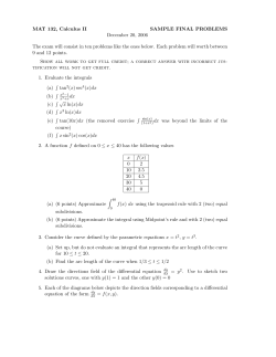


© Copyright 2026