
A high physical accuracy method for incompressible
A high physical accuracy method for incompressible
magnetohydrodynamics
Michael A. Case∗
Leo G. Rebholz‡
Alexander Labovsky
Nicholas E. Wilson§
†
Abstract
We present an energy, cross-helicity and magnetic helicity preserving method for
solving incompressible magnetohydrodynamic equations with strong enforcement of
solenoidal constraints. The method is a semi-implicit Galerkin finite element discretization, that enforces pointwise solenoidal constraints by employing the Scott-Vogelius
finite elements. We prove the unconditional stability of the method and the optimal
convergence rate. We also perform several numerical tests verifying the effectiveness
of our scheme and, in particular, its clear advantage over using the Taylor-Hood finite
elements.
1
Introduction
The conservation equations for incompressible magnetohydrodynamic (MHD) flows describe
conducting, non-magnetic fluids, such as salt water, liquid metals, plasmas and strong
electrolytes [7]. We will study finite element discretizations of the MHD equations in the
following form, originally developed by Ladyzhenskaya, and studied in, e.g., [10, 18, 11, 12,
17]:
s
ut + ∇ · (uuT ) − Re−1 ∆u + ∇(B · B) − s∇ · BB T + ∇p = f,
2
∇ · u = 0,
Bt +
Re−1
m ∇
× (∇ × B) + ∇ × (B × u) = ∇ × g,
∇ · B = 0.
(1.1)
(1.2)
(1.3)
(1.4)
Here, u is velocity, p is pressure, f is body force, ∇ × g is a forcing on the magnetic field B,
Re is the Reynolds number, Rem is the magnetic Reynolds number, and s is the coupling
number.
We study a semi-implicit Galerkin finite element discretization of (1.1)-(1.4) which enforces pointwise solenoidal velocity and magnetic fields, as well as global conservation of
∗
Department of Mathematical Sciences, Clemson University, Clemson, SC 29634, [email protected].
Partially supported by National Science Foundation grant DMS0914478.
†
Department of Scientific Computing, Florida State University, Tallahassee FL 32306, [email protected].
Partially supported by the US Air Force Office of Scientific Research under grant number FA9550-08-1-0415
‡
Department of Mathematical Sciences, Clemson University, Clemson, SC 29634, [email protected],
http://www.math.clemson.edu/∼rebholz. Partially supported by National Science Foundation grant
DMS0914478.
§
Department of Mathematical Sciences, Clemson University, Clemson, SC 29634, [email protected].
Partially supported by National Science Foundation grant DMS0914478.
1
energy and cross-helicity; by global conservation we mean the quantities are unchanged
for ideal MHD with periodic boundary conditions, and in the viscous/resistance case and
more general boundary conditions the quantities are exactly balanced, analogous to the
continuous case. We also prove the exact conservation of magnetic helicity for the ideal
MHD system, thus showing that our model preserves all three physical quantities that are
conserved in the ideal MHD. In addition to proving these conservation laws, we also prove
the scheme is unconditionally stable, well-posed, and optimally convergent. Lastly, several
numerical experiments are given that demonstrate the effectiveness of the scheme.
Most schemes for fluid flow simulation conserve energy, but other fundamental conservation laws are often ignored or not strongly enforced. However, when these other laws are
correctly accounted for in the numerical scheme, resulting solutions have greater physical
accuracy, which leads to longer time stability and accuracy. For example, Arakawa’s scheme
for the 2D Navier-Stokes equations(NSE) that conserves energy and enstrophy[1], Arakawa
and Lamb’s scheme for the shallow water equations that conserves enstrophy and potential
enstrophy [2] and those of Navon [19, 20], J.G. Liu and W. Wang’s finite difference schemes
for 3D axi-symmetric NSE flow that conserves energy and helicity [17] and MHD flows with
symmetry that conserve energy and cross-helicity, and most recently a scheme for full 3D
NSE that conserves energy and helicity [21, 6], all exhibit better long time behavior than
comparable schemes that conserve only energy. The discretization we formulate and study
herein for (1.1)-(1.4) is a finite element scheme that conserves all three fundamental quantities for general MHD flows - energy, cross-helicity and magnetic helicity, and is therefore
also expected to exhibit good accuracy.
In addition to integral invariants, there are other conservation laws fundamental to the
system (1.1)-(1.4), which are explicitly part of the continuous system as equations (1.2)
and (1.4). Finite element discretizations typically enforce these laws weakly, however in
MHD this is typically not sufficient. The problems that can arise from a poor enforcement
of ∇ · u = 0 are well known even for the simpler problems such as steady Navier-Stokes
equations (NSE), see e.g. [15], and thus in the MHD system such physically inconsistent
effects can be magnified. The requirement that ∇ · B = 0 comes from the fact that B
is derived as the curl of a electric field, and since div curl = 0 is a formal mathematical
identity, for B not to be divergence free is mathematical inconsistency. This is well known
in the MHD community, and algorithms that preserve incompressibility of B provided an
incompressible initial condition is given exist [18], and for those that do not, techniques such
as ‘divergence cleansing’ can be applied to recover mathematically plausible solutions [8].
The problem of satisfying the divergence-free condition for the magnetic field is crucial in
many of the MHD applications; for instance, different numerical techniques have been used
to prevent the incorrect shock capturing because of the violation of ∇ · B = 0 condition.
One can find the description of such techniques in [23] and references therein. Our scheme
strongly enforces (pointwise!) the solenoidal constraints by coupling the discrete analog of
(1.4) to (1.3) through the addition of a corresponding Lagrange multiplier λ to (1.3), then
using the Scott-Vogelius element pair to approximate both (u, p) and (B, λ). Under mild
restrictions, this element pair has recently been shown to be LBB stable and admits optimal
approximation properties, and also implicitly enforces strong divergence free constraints
when only weak enforcement is implemented [24]. It has since been successfully used with
the steady and time-dependent NSE [4, 16, 15, 5], and thus the extension to using it for
MHD is a next natural step.
There are two natural extensions of the scheme given in Section 3 for which our analysis
is relevant. The first is for a linearization of the scheme via the method of Baker [3],
2
by linearly extrapolating the first term of the each of the four trilinear terms. All of the
theory proven for the full nonlinear (Crank-Nicolson) scheme is still valid, although the
convergence proof would have additional technical details. This scheme offers a significant
increase in efficiency, since only one linear solve is needed at each timestep; all of our
numerical experiments with the scheme will employ this linearization. The second extension
is for Taylor-Hood elements, provided the trilinear terms are all skew-symmetrized. Here,
the global conservation of energy and cross helicity still hold as does optimal convergence,
however with this element choice, the incompressibility constraints are only weakly enforced.
We show with a simple numerical example that, as expected, this element choice can give
much worse results that Scott-Vogelius elements provide.
This report is arranged as follows. Section 2 presents notation and preliminaries, Section
3 derives the numerical scheme and proves conservation properties for it. Section 4 presents
stability and convergence analysis for the scheme, and Section 5 discusses extensions of
the scheme to a linearized form that still admits the conservation properties, and to the
choice of Taylor-Hood elements. Section 6 gives several numerical experiments that show
the effectiveness of the scheme.
2
Notation and Preliminaries
We consider a polygonal or polyhedral domain Ω ⊂ Rd (d = 2 or 3), with Dirichlet boundary
conditions for both velocity and the magnetic field. We denote the L2 (Ω) norm and inner
product by ∥·∥ and (·, ·), respectively.
For simplicity, we consider the case of homogeneous Dirichlet conditions, but the extension to the general case can be made in the standard way [22]. Extension to periodic
boundaries is trivial, but requires the domain be a box, and extension to most other boundary conditions is done in the usual way.
The Poincare-Freidrich’s inequality will be used throughout our analysis: For ϕ ∈
H01 (Ω),
∥ϕ∥ ≤ C(Ω) ∥∇ϕ∥ .
The natural function spaces for our problem are
X = H01 (Ω) = {v ∈ H 1 (Ω) : v = 0 on ∂Ω}
∫
2
2
Q = L0 (Ω) = {q ∈ L (Ω) :
q = 0}
Ω
The following lemma for bounding the trilinear forms will be used heavily in our analysis.
Lemma 2.1. For u, v, w ∈ X, there exists C = C(Ω) such that
(u · ∇v, w) ≤ C ∥∇u∥ ∥∇v∥ ∥v∥1/2 ∥∇v∥1/2
(2.1)
(u · ∇v, w) ≤ C ∥∇u∥ ∥∇v∥ ∥∇v∥
(2.2)
Proof. These estimates follow from Holder’s inequality, the Sobolev imbedding theorem and
Poincare-Freidrich’s inequality.
The finite element spaces used throughout will be the Scott-Vogelius pair, (Xh , Qh ) =
disc ). We make the following two assumptions throughout this report:
(Pk , Pk−1
A1: The mesh is created as a barycenter refinement of a regular mesh,
A2: The polynomial degree k ≥ d.
3
Under these assumptions, this element pair is LBB stable and admits optimal approximation
properties [24]. This pair will be used to approximate the velocity-pressure pair, and the
magnetic field - Lagrange multiplier pair. A fundamentally important property of ScottVogelius elemetns is that the usual weak enforcement of incompressibility via
(∇ · vh , qh ) = 0 ∀qh ∈ Qh ,
implicitly enforces incompressibility pointwise since qh can be chosen as qh = ∇ · vh , which
provides
∥∇ · vh ∥2 = 0 =⇒ ∇ · vh = 0.
This property is important in the proposed numerical scheme for several reasons. First, mass
conservation can be enforced pointwise via the usual weak enforcement of incompressibility
of velocity. Second, the incompressibility of the magnetic field can be enforced pointwise in
the same manner. Third, in all of our trilinear terms, skew-symmetry need not be enforced
(for stability) as it would if, for example, Taylor-Hood elements were used; this provides
a cheaper assembly time. Last, the use of Scott-Vogelius elements decouples the pressure
error from the velocity error. The pressure in the numerical scheme we study is actually a
modified pressure P := p + 2s |B|2 (see below for more details), which can be significantly
more complex than usual pressure. However, with Scott-Vogelius elements, larger pressure
errors do not directly affect the velocity error as they do for most other common element
choices [13, 14].
Define the space of discretely divergence free function as
Vh := {vh ∈ Xh : (∇ · vh , qh ) = 0 ∀qh ∈ Qh }.
Note that functions in Vh , when using the Scott-Vogelius pair, are pointwise divergence free.
3
Derivation of energy and helicities conserving scheme
There are three fundamental physical quantities conserved in the ideal MHD (in the absence
of the forcing, with zero kinematic viscosity and magnetic diffusivity). These are the energy,
cross-helicity and magnetic helicity, defined, respectively, as
∫
1
E =
(u(x) · u(x) + sB(x) · B(x))dx,
2 Ω
∫
1
HC =
(u(x) · B(x))dx,
2 Ω
∫
1
(A(x) · B(x))dx,
HM =
2 Ω
where A is the vector potential, B = ∇×A. We shall verify that all three of these quantities
are conserved by our scheme.
We begin with the formulation (1.1)-(1.4), expand the curl operator in the (1.3) equation
and use that ∇ · u = ∇ · B = 0 to get
s
ut − Re−1 ∆u + u · ∇u + ∇(B · B) − sB · ∇B + ∇p = f
2
∇·u = 0
Bt +
Re−1
m ∇
× (∇ × B) + u · ∇B − B · ∇u = ∇ × g
∇·B = 0
4
(3.1)
(3.2)
(3.3)
(3.4)
Denoting the modified pressure P := p + 2s |B|2 , using the vector identity
∆B = −∇ × (∇ × B) + ∇(∇ × B),
and defining λ := Rem ∇ · B(= 0) to act as a Lagrange multiplier corresponding to the
solenoidal constraint of the magnetic field, we get
ut − Re−1 ∆u + u · ∇u − sB · ∇B + ∇P
Bt −
Re−1
m ∆B
= f
(3.5)
∇·u = 0
(3.6)
+ u · ∇B − B · ∇u − ∇λ = ∇ × g
(3.7)
∇·B = 0
(3.8)
The numerical scheme is now derived with a Galerkin finite element spatial discretization
n+ 1
and (four leg) trapezoidal time discretization. Denote uh 2 := 21 (unh +un+1
h ). We require the
discrete initial conditions to be pointwise divergence free, that is, u0h and Bh0 must be in Vh .
n+ 12
n+1
Then ∀(vh , χh , qh , rh ) ∈ (Xh , Xh , Qh , Qh ) find (un+1
, ph
h , Bh
T
for n = 0, 1, 2, ..., M = ∆t
n+ 12
, λh
) ∈ (Xh , Xh , Qh , Qh )
1 n+1
n+ 1
n+ 1
n+ 1
(uh − unh , vh ) + (uh 2 · ∇uh 2 , vh ) + Re−1 (∇uh 2 , ∇vh )
∆t
n+ 12
−s(Bh
n+ 12
· ∇Bh
n+ 12
, vh ) − (Ph
1
(B n+1 − Bhn , χh ) + Re−1
m (∇Bh
∆t h
n+ 12
+(uh
n+ 12
· ∇Bh
1
, ∇ · vh ) = (f (tn+ 2 ), vh )
(3.9)
(∇ · un+1
h , qh ) = 0
1
n+
n+ 1
(Bh 2 · ∇uh 2 , χh )
(3.10)
n+ 12
, ∇χh ) −
n+ 12
, ∇ · χh ) = (∇ × g(tn+ 2 ), χh )
, χh ) + (λh
1
(∇ ·
Bhn+1 , rh )
=0
(3.11)
(3.12)
Lemma 3.1. Solutions to the scheme (3.9)-(3.12) admit the following conservation laws:
• Mass conservation
∇ · unh = 0 (pointwise)
(3.13)
• Incompressibility of the magnetic field
∇ · Bhn = 0 (pointwise)
(3.14)
• Global energy conservation
(
)
(
2 )
M
−1
∑
n+ 1 2
1 M 2 s M 2
n+ 12 −1
−1
2
u + B + ∆t
Re h
∇uh + sRem ∇Bh 2 h 2
n=0
(
)
)
M
−1 (
∑
1
s
n+ 12
n+ 21
n+ 12
0 2
0 2
n+ 12
=
u
+
Bh
+ ∆t
(f (t
), uh ) + s(∇ × g(t
), Bh )
2 h
2
n=0
(3.15)
5
• Global cross-helicity conservation
M
(uM
h , Bh )
+ ∆t
M
−1 (
∑
(Re
−1
n=0
=
(u0h , Bh0 )
+ ∆t
)
+
n+ 1
n+ 12
Re−1
, ∇Bh 2 )
m )(∇uh
M
−1 (
∑
n+ 12
(∇ × g(t
n+ 1
), uh 2 )
+ (f (t
n+ 12
)
n+ 1
), Bh 2 )
(3.16)
n=0
Hence for f = g = 0 and Re = Rem = ∞, we have exact conservation of both energy
and cross-helicity.
• Global magnetic helicity conservation in the case of ideal MHD
0
0
(BhM , AM
h ) = (Bh , Ah ), where A is the vector potential, B = ∇ × A.
(3.17)
Proof. First, we note that for Scott-Vogelius elements, we can choose qh = ∇ · un+1
and
h
n+1/2
n+1
n+1
n+1
rh = ∇ · Bh . Hence we have that ∇ · uh = ∇ · Bh = 0, and thus that ∇ · uh
=
n+1/2
∇ · Bh
= 0. This proves the first two conservation laws, and moreover these results will
be used in the proofs of the other laws.
n+ 1
n+ 1
To prove energy conservation choose vh = uh 2 and χh = Bh 2 which vanishes the
second, fourth, and sixth terms in (3.9) and the fourth and fifth terms in (3.11), leaving
)
1
1
1
1 2
1 (
un+1 2 − ∥un ∥2 + Re−1 ∇un+ 2 − s(B n+ 2 · ∇B n+ 2 , un+ 2 )
h
h
h
h
h
h
2∆t
1
n+ 12
= (f (tn+ 2 ), uh
),
2
(
)
1
1
1
1 n+ 12 B n+1 2 − ∥B n ∥2 + Re−1
− (B n+ 2 · ∇un+ 2 , B n+ 2 )
m ∇Bh
h
h
h
h
h
2∆t
n+ 12
1
= (∇ × g(tn+ 2 ), Bh
n+ 12
Multiplying (3.19) by s, rewriting the nonlinear term in (3.18) as −s(Bh
n+ 1
s(Bh 2
·
n+ 1
n+ 1
∇uh 2 , Bh 2 ),
(3.18)
(3.19)
).
n+ 12
·∇Bh
n+ 21
, uh
)=
and adding (3.18) and (3.19) gives
2
n+1 2
n+ 1 2
1 s
2
n+1
n
n
−1
2
(uh − ∥uh ∥) +
(Bh − ∥Bh ∥ ) + Re ∇uh 2∆t
2∆t
2
1
1
n+ 12 = (f (tn+ 12 ), un+ 2 ) + s(∇ × g(tn+ 12 ), B n+ 2 ).
∇B
+sRe−1
m h
h
h
(3.20)
Multipling by ∆t and summing over timesteps finishes the proof of (3.15).
n+ 1
n+ 1
To prove cross helicity is conserved we choose vh = Bh 2 in (3.9) and χh = uh 2 in
(3.11). This vanishes the fourth and fifth terms in (3.9) and third and fifth terms in (3.9),
leaving
6
1 n+1
n+ 1
n+ 1
n+ 1
n+ 1
n+ 1
n+ 1
(uh − unh , Bh 2 ) + (uh 2 · ∇uh 2 , Bh 2 ) + Re−1 (∇uh 2 , ∇Bh 2 )
∆t
n+ 12
1
= (f (tn+ 2 ), Bh
),
1
1
1
1
1
1
1
n+
n+
n+
n+
n+
n+
2
(B n+1 − Bhn , uh 2 ) + Re−1
, ∇uh 2 ) + (uh 2 · ∇Bh 2 , uh 2 )
m (∇Bh
∆t h
n+ 12
1
= (∇ × g(tn+ 2 ), uh
).
(3.21)
(3.22)
Adding (3.21) and (3.22) and noting that:
n+ 12
(uh
n+ 12
· ∇uh
n+ 12
, Bh
n+ 12
) = −(uh
n+ 12
· ∇Bh
n+ 12
, uh
), and
(3.23)
1 n+1
1
n+ 1
n+ 1
(uh − unh , Bh 2 ) +
(Bhn+1 − Bhn , uh 2 )
(3.24)
∆t
∆t
)
)
1 ( n+1 n+1
1 ( n+1 n
=
(uh , Bh ) − (unh , Bhn ) +
(uh , Bh ) − (unh , Bhn+1 )
(3.25)
2∆t
2∆t
)
)
1 ( n+1 n+1
1 ( n+1 n
+
(Bh , uh ) − (Bhn , unh ) −
(Bh , uh ) − (Bhn , un+1
) , (3.26)
h
2∆t
2∆t
we get
)
1 ( n+1 n+1
n+ 1
n+ 12
(uh , Bh ) − (unh , Bhn ) + (Re−1 + Re−1
, ∇Bh 2 )
m )(∇uh
∆t
1
n+ 21
= (∇ × g(tn+ 2 ), uh
n+ 12
1
) + (f (tn+ 2 ), Bh
)
(3.27)
Multiplying by ∆t and summing over timesteps finishes the proof of (3.16).
n+ 12
Finally, choose χh = Ah
diffusivity we obtain
in (3.11). In the absence of forcing and with zero magnetic
1
n+ 1
n+ 1
n+ 1
n+ 1
n+ 1
n+ 1
n+ 1
(Bhn+1 − Bhn , Ah 2 ) + (uh 2 · ∇Bh 2 , Ah 2 ) − (Bh 2 · ∇uh 2 , Ah 2 ) = 0. (3.28)
∆t
We will use the identity
((∇ × v) × u, w) = (u · ∇v, w) − (w · ∇v, u).
(3.29)
Since the cross-product of two vectors is orthogonal to each of them,
n+ 12
((∇ × Ah
n+ 12
) × uh
n+ 12
, ∇ × Ah
(3.30)
) = 0.
It follows from (3.30) and (3.29) that
n+ 12
(uh
n+ 12
Since Bh
n+ 12
· ∇Ah
n+ 12
= ∇ × Ah
n+ 12
, ∇ × Ah
n+ 12
) = ((∇ × Ah
n+ 12
) · ∇Ah
, we obtain
1
(B n+1 − Bhn , An+1
+ Anh ) = 0,
h
2∆t h
and therefore
n+1
n
n
(∇ × An+1
h , Ah ) = (∇ × Ah , Ah ),
which completes the proof.
7
n+ 12
, uh
).
(3.31)
4
Numerical analysis of the scheme
We prove in this section that the scheme is both unconditionally stable and optimally
convergent.
Lemma 4.1. Solutions to the scheme (3.9)-(3.12) are stable provided f ∈ L2 (0, T ; H −1 (Ω))
and g ∈ L2 (0, T ; L2 (Ω)), and satisfy
(
2 )
M
−1
( 2
∑
M 2 )
n+ 1 2
n+ 12 −1
M
−1
2
u + s B + ∆t
Re h
h
∇uh + sRem ∇Bh n=0
M
−1 (
)
( ∑
0 2 )
n+ 12 2
n+ 12 2
0 2
≤ u h + s Bh
) + sRem g(t
) = C(Re, Rem , f, g).
+∆t
Re f (t
−1
n=0
(4.1)
Proof. We begin this proof with the energy conservation equality (3.15),
(
)
(
)
M
−1
∑
1 2
1 M 2 s M 2
n+ 1 2
n+
−1
−1
2
2
u + B + ∆t
Re h
2 h ∇uh + sRem ∇Bh 2
n=0
(
)
)
M
−1 (
∑
1
s
n+ 12
n+ 21
0 2
0 2
n+ 12
n+ 12
), uh ) + s(∇ × g(t
), Bh )
=
u
+
Bh
+ ∆t
(f (t
(4.2)
2 h
2
n=0
The forcing term can be majorized with Cauchy-Schwarz and Young’s inequalities to get
1
n+ 12
(f (tn+ 2 ), uh
)≤
Re Re−1 n+ 12 2
n+1/2 2
) +
f (t
∇uh
,
2
2
−1
(4.3)
and similarly for the magnetic forcing term,
s(∇ × g(t
n+ 12
n+ 1
), Bh 2 )
sRem n+ 12 2 sRe−1
m
≤
) +
g(t
2
2
1 2
∇B n+ 2 .
h
(4.4)
Using (4.3) and (4.4) in (4.2) gives
(
2 )
M
−1
( 2
∑
M 2 )
n+ 1 2
n+ 12 M
−1
−1
2
u + s B + ∆t
Re h
h
∇uh + sRem ∇Bh n=0
M
−1 (
)
( ∑
0 2 )
n+ 21 2
n+ 12 2
0 2
≤ uh + s Bh
+ ∆t
) + sRem g(t
) , (4.5)
Re f (t
−1
n=0
which proves the lemma.
We now prove convergence of the scheme.
Theorem 4.1. Assume (u, p, B) solves (1.1)-(1.4) and satisfying Bt , ut ∈ L2 (Ω, [0, T ]),
Btt , utt ∈ L2 (Ω, [0, T ]), Bttt , uttt ∈ L2 (Ω, [0, T ]), and B, u ∈ L∞ (0, T ; H m (Ω)), where m =
max (3, k). Then the solution (uh , ph , Bh , λh ) to (3.9)-(3.12) converges to the true solution
with optimal rate
∥u − uh ∥2,1 + ∥B − Bh ∥2,1 = O(∆t2 + hk ).
8
Proof. Multiply the momentum and magnetic equations (1.1), (1.3) at tn+1/2 by vh ∈ Vh and
χh ∈ Vh , respectively, and integrate over the domain. Denoting eku = ukh −uk , ekB = Bhk −B k ,
we get
(ut (tn+ 2 ), vh ) + (u(tn+ 2 ) · ∇u(tn+ 2 ), vh ) + Re−1 (∇u(tn+ 2 ), ∇vh )
1
1
1
1
1
1
(4.6)
1
− s(B(tn+ 2 ) · ∇B(tn+ 2 ), ∇ · vh ) = (f (tn+ 2 ), vh ))
n+ 2
(Bt (tn+ 2 ), χh ) + Re−1
), ∇χh ) − (B(tn+ 2 ) · ∇u(tn+ 2 ), χh )
m (∇B(t
1
1
1
1
1
1
(4.7)
1
+ (un+ 2 · ∇B n+ 2 , χh ) = (∇ × g(tn+ 2 ), χh ).
As usual, we will look to subtract the continuous formulation of the variational problem
from the discrete formulation. We start this process by introducing the following terms
(4.8)-(4.11), which replace the terms in the left-hand side of (4.6). To simplify notation, we
use ± to denote adding and subtracting the same term.
1
(ut (tn+ 2 ), vh ) ±
1
1
1
(u(tn+1 ) − u(tn ), vh ) =
(u(tn+1 ) − u(tn ), vh )
∆t
∆t
1
+ (ut (tn+ 2 ) − {u(tn+1 ) − u(tn )}∆t−1 , vh ).
1
1
1
1
1
(4.8)
1
(u(tn+ 2 ) · ∇u(tn+ 2 ), vh ) ± (un+ 2 · ∇un+ 2 , vh ) = (u(tn+ 2 ) · ∇(u(tn+ 2 ) − un+ 2 ), vh )
1
1
1
1
1
+ ((u(tn+ 2 ) − un+ 2 ) · ∇un+ 2 , vh ) + (un+ 2 · ∇un+ 2 , vh ).
(4.9)
(
)
1
1
Re−1 (∇u(tn+ 2 ), ∇vh ) ± (∇un+ 2 , ∇vh )
= Re−1 (∇(u(tn+ 2 ) − un+ 2 ), ∇vh ) + Re−1 (∇un+ 2 , ∇vh ) (4.10)
1
1
1
1
1
1
1
1
1
1
−s(B(tn+ 2 ) · ∇B(tn+ 2 ), vh ) ± s(B n+ 2 · ∇B n+ 2 , vh ) = s(B n+ 2 · ∇(B n+ 2 − B(tn+ 2 )), vh )
1
1
1
1
1
+ s((B n+ 2 − B(tn+ 2 )) · ∇B(tn+ 2 ), vh ) − s(B n+ 2 · ∇B n+ 2 , vh ).
(4.11)
Now we can directly subtract (4.6) from (3.9),
1
1 n+1
n+ 1
n+ 1
n+ 1
n+ 1
(eu − enu , vh ) + Re−1 (∇eu 2 , ∇vh ) + (uh 2 · ∇eu 2 , vh ) + (eu 2 · ∇un+ 2 , vh )
∆t
n+ 21
− s(Bh
n+ 12
· eB
n+ 12
, vh ) − s(Bh
n+ 12
] · ∇eB
n+ 12
, vh ) − s(eB
1
· ∇B n+ 2 , vh )
= (ut (tn+ 2 ) − {u(tn+1 ) − u(tn )}∆t−1 , vh ) + Re−1 (∇(u(tn+ 2 ) − un+ 2 ), ∇vh )
1
1
1
1
1
1
1
1
1
+ (u(tn+ 2 ) · ∇(u(tn+ 2 ) − un+ 2 ), vh ) + ((u(tn+ 2 ) − un+ 2 ) · ∇un+ 2 , vh )
1
1
1
1
1
1
+s((B n+ 2 −B(tn+ 2 ))·∇B(tn+ 2 ), vh )+s(B n+ 2 ·∇(B n+ 2 − B(tn+ 2 )), vh ) =: G1 (t, B, u, vh )
(4.12)
Note that G1 represents terms associated with interpolation error and are introduced
to simplify the notation. Using the assumptions on the regularity of the solution, analysis
similar to that in Chapter 3 will show
G1 (t, B, u, vh ) ≤ C∆t2 ∥vh ∥.
9
(4.13)
Similar to the derivation of (4.12) we introduce terms (4.14)-(4.15) to the left hand side
of (4.7) and then subtract from (3.11).
1
1
1
1
1
1
1
−(B(tn+ 2 ) · ∇u(tn+ 2 ), χh ) ± (B n+ 2 · ∇un+ 2 , χh ) = (B(tn+ 2 ) · ∇(un+ 2 − u(tn+ 2 )), χh )
1
1
1
+ ((B n+ 2 − B(tn+ 2 )) · ∇un+ 2 , χh )
1
1
− (B n+ 2 · ∇un+ 2 , χh ).
(4.14)
1
1
1
1
1
(u(tn+ 2 ) · ∇(B(tn+ 2 ) − B n+ 2 ), χh ) ± (un+ 2 · ∇B n+ 2 , χh )
1
1
1
1
1
1
= (u(tn+ 2 ) · ∇(B(tn+ 2 ) − B n+ 2 ), χh ) + ((u(tn+ 2 ) − un+ 2 ) · ∇B n+ 2 , χh )
1
1
+ (un+ 2 · ∇B n+ 2 , χh ) (4.15)
1 n+1
n+ 12
n+ 12
n+ 12
(eB − enB , χh ) + Re−1
(∇e
,
∇χ
)
−
(B
·
∇e
, χh )
u
h
m
B
h
∆t
n+ 12
− (eB
1
n+ 12
1
· ∇un+ 2 , χh ) + (un+ 2 · ∇eB
n+ 12
, χh ) + (eu
1
· ∇B n+ 2 , χh )
= (Bt (tn+ 2 ) − {B(tn+1 ) − B(tn )}∆t−1 , χh )
1
n+ 2
+ Re−1
) − B n+ 2 ), ∇χh )
m (∇(B(t
1
1
1
1
1
1
1
1
1
1
+ (B(tn+ 2 ) · ∇(un+ 2 − u(tn+ 2 )), χh ) + ((B n+ 2 − B(tn+ 2 )) · ∇un+ 2 , χh )
1
1
1
1
+ (u(tn+ 2 ) · ∇(B(tn+ 2 ) − B n+ 2 ), χh ) + ((u(tn+ 2 ) − un+ 2 ) · ∇B n+ 2 , χh )
= G2 (t, B, u, χh )
(4.16)
Similar to G1 , we bound G2 by
G2 (t, B, u, vh ) ≤ C∆t2 ∥χh ∥.
(4.17)
Define ϕnh = (unh − U n ) and η n = (un − U n ) ⇒ enu = ϕnh − ηun and analogously enB =
n . Where U k ∈ V and B k ∈ V . Substituting into (4.12)
− B n ) + (B n − B n ) = ψhn − ηB
h
h
and (4.16) results in:
(Bhn
1
1 n+1
n+ 1
n+ 1
n+ 1
n+ 1
(ϕh − ϕnh , vh ) + Re−1 (∇ϕh 2 , ∇vh ) + (uh 2 · ∇ϕh 2 , vh ) + (ϕh 2 · ∇un+ 2 , vh )
∆t
n+ 12
− s(Bh
=
n+ 12
· ∇ψh
n+ 12
, vh ) − s(ψh
1
· ∇B n+ 2 , vh )
1 n+1
n+ 1
n+ 1
n+ 1
(ηu − ηun , vh ) + Re−1 (∇ηu 2 , ∇vh ) + (uh 2 · ∇ηu 2 , vh )
∆t
n+ 21
+ (ηu
n+ 21
− s(ηB
n+ 12
1
· ∇un+ 2 , vh ) − s(Bh
n+ 12
· ηB
n+ 12
, vh ) − s(Bh
n+ 12
· ∇ηB
, vh )
1
· ∇B n+ 2 , vh ) + G1 (t, u, B, vh )
(4.18)
10
1
1
n+ 1
n+ 1
n+ 1
n+1
(ψhn+1 − ψhn , χh ) + Re−1
, ∇χh ) − (Bh 2 · ∇ϕh 2 , χh ) − (ψh 2 · ∇un+ 2 , χh )
m (∇ψh
∆t
n+ 12
1
+ (un+ 2 · ∇ψh
=
n+ 12
, χh ) + (ϕh
1
· ∇B n+ 2 , χh )
1 n+1
n+ 12
n+ 21
n+ 12
n
, χh ) + Re−1
(∇η
,
∇χ
)
−
(B
(ηB − ηB
·
∇η
, χh )
u
h
m
B
h
∆t
n+ 12
− (ηB
1
n+ 12
1
· ∇un+ 2 , χh ) + (un+ 2 · ∇ηB
n+ 21
, χh ) + (ηu
1
· ∇B n+ 2 , χh )
+ G2 (t, u, B, χh )
(4.19)
n+ 12
Taking χh = ψh
n+ 12
and vh = ϕh
into (4.18) and (4.19) and simplifying yields
1 2
1
1
2
1 − ∥ϕn ∥2 ) + Re−1 ∇ϕn+ 2 + (ϕn+ 2 · ∇un+ 12 , ϕn+ 2 )
(ϕn+1
h
h
h
h
h
2∆t
n+ 12
− s(Bh
n+ 12
· ∇ψh
n+ 12
n+ 12
) − s(ψh
n+ 12
1
· ∇B n+ 2 , ϕh
)
1
1
1
1
1
1 n+1
n+
n+
n+
n+
n+
n+ 1
=
(ηu − ηun , ϕh 2 ) + Re−1 (∇ηu 2 , ∇ϕh 2 ) + (uh 2 · ∇ηu 2 , ϕh 2 )
∆t
n+ 12
+ (ηu
−
, ϕh
n+ 12
1
· ∇un+ 2 , ϕh
n+ 1
s(ηB 2
· ∇B
n+ 21
) − s(Bh
n+ 1
, ϕh 2 )
n+ 12
+
n+ 12
· ∇ηB
n+ 12
, ϕh
)
n+ 1
G1 (t, u, B, ϕh 2 )
(4.20)
2 2
n+ 1 2
1 n+ 12
n+ 12
n+ 21
n+ 12
n+ 12 n+ 12
n+ 12 n+ 12
−1 2
(ψh −ψh )+Rem ∇ψh ·∇ϕ
,
ψ
)−(ψ
·∇u
,
ψ
)
−(B
h
h
h
h
h
2∆t
1
1 n+1
n+ 1
n+ 1
n+ 1
n+ 12
n+ 1
n
+ (ϕh 2 · ∇B n+ 2 , ψh 2 ) =
(ηB − ηB
, ψh 2 ) + Re−1
, ∇ψh 2 )
m (∇ηB
∆t
n+ 12
− (Bh
n+ 12
· ∇ηu
n+ 12
, ψh
n+ 12
) − (ηB
1
n+ 12
· ∇un+ 2 , ψh
n+ 12
+ (ηu
1
1
n+ 12
) + (un+ 2 · ∇ηB
n+ 21
· ∇B n+ 2 , ψh
n+ 12
, ψh
n+ 12
) + G2 (t, u, B, ψh
)
) (4.21)
Using the inequality,
1 n+1
1
n+ 1
(η
− ηun , ϕh 2 ) ≤
∆t
2∆t
∫
tn+1
tn
11
2
1
n+ 12 ,
∥∂(ηu )∥ dt + ϕ
2 h 2
(4.22)
along with H¨older’s Inequality and (4.13),
−1 1 2
2
1 − ∥ϕn ∥2 ) + Re ∇ϕn+ 2 (ϕn+1
h
h
2∆t
2 h 2 ( −1 ) ∫ tn+1
n+ 1 2
1
1
Re
n+ 21 2
2
∥∂t (ηu )∥ dt + ϕh +
≤
ηu 2∆t tn
2
2
2
1
1
n+ 12 n+ 12
n+ 12
n+ 12
n+ 21 n+ 12 n+ 2 n+ 2 + ∇u
ϕh + s(Bh · ∇ψh , ϕh ) + s ∇B
ψh ϕh ∞
∞
1
1
n+ 1 n+ 1 n+ 1 n+ 1 n+ 2
n+ 12 n+ 12 n+ 12 n+ 2
2
2
2
+C ∇uh ∇ηu ∇ϕh +∇u 2 ∞ ηu ϕh +Cs ∇Bh ∇ηB ∇ϕh 1
1
1
n+ 12 n+ 2 n+ 2 2 n+ 2 + s ∇B
ηB ϕh + C∆t ϕh (4.23)
∞
This reduces, with Cauchy-Schwarz and Young’s inequalities and the assumption of the
regularity of the solution, to
2
( −1 ) ∫ tn+1
n+ 1 2
1 Re−1 1
Re
n+ 12 2
n+1 2
n 2
2
( ϕh
− ∥ϕh ∥ ) +
∇ϕ
≤
∥∂t (ηu )∥ dt +
ηu 2∆t
4 h 2∆t tn
2
2 2
1 2
n+ 1 2 n+ 1 2
n+ 1 2 n+ 1 2 2 n+ 12 n+ 12 4 n+ 2 2
2
2 2
+C(ϕh + ψh +∆t + ηu + ∇uh ∇ηu +s ∇Bh ∇ηB 2
n+ 1 n+ 12
n+ 12
n+ 12
2
+ s2 ·
∇ψ
,
ϕ
) (4.24)
η
)
+
s(B
h
h
h
B We now step back from (4.24) and return to (4.21), which implies
∫ tn+1
2
1 1
Re−1
n+1/2 2
m (ψhn+1 − ∥ψhn ∥2 ) +
∇ψ
≤
∥∂t (ηB )∥2 dt
h
2∆t
2
2∆t tn
2
n+ 1 2
n+ 1 n+ 1 1
1
n+ 21
n+ 12
n+ 12 n+ 12
−1
n+
2
2
2
+ Rem ∇η
+ ψ
B + (Bh · ∇ϕh , ψh ) + ∇B 2 ∞ ϕh ψh 2 h 2
n+ 1 n+ 1 1
n+ 12 n+ 12 n+ 12 n+ 12 n+ 21 n+
2
2
+∇u
ψh +C ∇Bh ∇ηu ∇ψh +C ∇u 2 ∞ ∇ηB ψh ∞
1
1
1
n+ 12 n+ 2 n+ 2 2 n+ 2 + ∇B
ηu ψh + C∆t ψh . (4.25)
∞
Under the regularity assumptions, Cauchy-Schwarz and Young’s inequalities, this can
be reduced to
∫ tn+1
2
2
Re−1
1
1 m (ψhn+1 − ∥ψhn ∥2 ) +
∇ψhn+1 ≤
∥∂t (ηB )∥2 dt
2∆t
4
2∆t tn
n+ 1 2 n+ 1 2 n+ 1 2
n+ 1 2
n+ 1 2
4
−1 2
2
2
2
2
+ Rem ∇ηB + C(
ψh + ∆t + ϕh + ∇ηB + ηu 2 2
n+ 21 n+ 12 n+ 12
n+ 21
n+ 12
+ Re ∇Bh ∇ηu ) + (Bh · ∇ϕh , ψh ). (4.26)
Multiplying (4.26) by s and adding it to (4.24), and using that
n+ 12
(Bh
n+ 12
· ∇ϕh
n+ 12
, ψh
n+ 12
) = −(Bh
12
n+ 12
· ∇ψh
n+ 12
, ϕh
),
along with the Poincare inequality and reducing, we get
2
−1 s Re−1 1 n+ 12 n+1/2 2
n+1 2
n+1 2
n 2
n 2
+ sRem ( ϕh
− ∥ϕh ∥ ) +
( ψh
− ∥ψh ∥ ) +
∇ϕ
∇ψ
h
2∆t
2∆t
4 h 4
( −1 ) ∫ tn+1
∫ tn+1
n+ 1 2
n+ 1 2
1
s
Re
2
2
−1
2
2
ηu +sRem ∇η
≤
∥∂t (ηu )∥ dt+
∥∂t (ηB )∥ dt+
B 2∆t tn
2∆t tn
2
2 2
n+ 1 2 n+ 1 2 n+ 1 2 n+ 1 2 n+ 1 2
n+ 12 n+ 12 4
2
2
2
2
2
+C(s)(
ϕh + ψh +∆t + ηu + ∇uh ∇ηu + ∇Bh ∇ηB 2 2
n+ 1 2
n+ 12 n+ 12 2
+
∇ηB + Re ∇Bh ∇ηu ) (4.27)
Multiplying by 2∆t and summing over timesteps now gives
(
2 )
−1
∑
M 2
M 2 M
n+ 1 2
n+ 21 −1
−1
2
ϕ + s ψ +
Re h
h
∇ϕh + sRem ∇ψh ∫
≤
n=0
T
(
2
2
∥∂t (ηu )∥ + s ∥∂t (ηB )∥
)
4
dt + CT ∆t + C∆t
0
M
−1
∑
n=0
n+ 1 2 n+ 1 2
2
2
(∇ηu + ∇ηB 2 2 2 2
n+ 1 2 n+ 1 2 n+ 12 n+ 12 n+ 21 n+ 12 2 2
+ ∇uh ∇ηu + ∇Bh ∇ηB + ∇Bh ∇ηu )
+C
M
∑
2 n+1 2
+ ψ
) (4.28)
(ϕn+1
h
h
n=1
Next we use approximation properties of the spaces and the stability estimate, which
reduces (4.28) to
(
)
−1
∑
1 2
M 2
M 2 M
n+ 1 2
n+
−1
−1
2
2
ϕ + s ψ +
Re h
h
∇ϕh + sRem ∇ψh n=0
≤ C(∆t4 + h2k ) + C
M
∑
2 n+1 2
+ ψ
) (4.29)
(ϕn+1
h
h
n=1
Applying the Gronwall inequality followed by the triangle inequality completes the proof.
5
Variations of the scheme
There are variations of this scheme for which most or all of the proven theoretical results
still hold.
5.1
A linearization that maintains both physical and asymptotic accuracy
For many evolution equations, certain circumstances can allow linearizations can often be
solved instead of the full nonlinear system, provided the particular linearization maintains
stability and asymptotic accuracy. For the system (3.9)-(3.12) proposed herein, we found
a linearization that preserves all of the conservation properties proved above, as well as
13
unconditional stability and optimal accuracy. The linearization is in the spirit of Baker’s
NSE linearization [3], where the first term of the nonlinearity is a second order in time
extrapolation of known values. For the system (3.9)-(3.12), there are multiple nonlinear
terms, and if the first term in each uses the extrapolation of Baker, then all of the proofs
above will follow identically, except for convergence which will require slightly more work
due to the new terms. Denoting the known functions
3 n 1 n−1
u − u
,
2 h 2 h
3 n 1 n−1
,
B − B
2 h 2 h
e n :=
U
h
e n :=
B
h
the linearized scheme at each time step is given by, ∀(vh , χh , qh , rh ) ∈ (Xh , Xh , Qh , Qh ),
1
1
1 n+1
e n · ∇un+ 2 , vh ) + Re−1 (∇un+ 2 , ∇vh )
(uh − unh , vh ) + (U
h
h
h
∆t
1
1
s en
n+ 12
e n · ∇B n+ 2 , vh ) − (pn+ 2 , ∇ · vh ) = (f (tn+ 12 ), vh )
+ (Bh · Bh , ∇ · vh ) − s(B
h
h
h
2
(∇ · un+1
h , qh ) = 0
1
1
1
n+ 2
e n · ∇un+ 2 , χh )
(Bhn+1 − Bhn , χh ) + Re−1
, ∇χh ) − (B
m (∇Bh
h
h
∆t
1
1
e n · ∇B n+ 2 , χh ) + (λn+ 2 , ∇ · χh ) = (∇ × g(tn+ 12 ), χh )
+(U
h
h
h
(∇ ·
Bhn+1 , rh )
=0
(5.1)
(5.2)
(5.3)
(5.4)
−1
0
0
Since this is a 2 step method, defining u−1
h := uh and Bh := Bh is sufficient to maintain
all the theoretical results.
5.2
Computing the scheme with Taylor-Hood elements
With Taylor-Hood elements, an important difference is that the velocity and magnetic field
approximations will no longer be pointwise divergence free. Hence it will be necessary
for stability to skew-symmetrize the nonlinear terms, and to combine the pressure in the
momentum equation with the gradient term resulting from the nonlinear coupling of the
magnetic field term. If we define the skew-symmetric operator
1
1
b∗ (u, v, w) := (u · ∇v, w) − (u · ∇w, v),
2
2
and let Ph be a modified pressure term, we get the linear scheme, ∀(vh , χh , qh , rh ) ∈
(Xh , Xh , Qh , Qh ),
1
1
1 n+1
e n , un+ 2 , vh ) + Re−1 (∇un+ 2 , ∇vh )
(uh − unh , vh ) + b∗ (U
h
h
h
∆t
1
1
e n , B n+ 2 , vh ) − (P n+ 2 , ∇ · vh ) = (f (tn+ 12 ), vh )
−sb∗ (B
h
h
h
(∇ · un+1
h , qh ) = 0
1
1
n+
∗ e n n+ 2
2
Re−1
(∇B
,
∇χ
)
−
b
(
B
,
u
, χh )
h
m
h
h
h
1
(B n+1 − Bhn , χh ) +
∆t h
1
1
e n , B n+ 2 , χh ) + (λn+ 2 , ∇ · χh ) = (∇ × g(tn+ 12 ), χh )
+bast (U
h
h
h
(∇ ·
14
Bhn+1 , rh )
=0
(5.5)
(5.6)
(5.7)
(5.8)
Note that we could similarly derive the nonlinear scheme. All of the theoretical results
follow as in the case of SV elements, but with the following exceptions: The velocity and
magnetic fields will now only be weakly mass conservative, and the error estimate will now
depend on the pressure error, although asymptotically the accuracy will be the same.
6
Numerical experiments
Here we run several numerical experiments to demonstrate the effectiveness of the scheme.
6.1
Experiment 1: Convergence rate verification
To verify our code, we compute convergence rates for a problem with known solution on a
series of refined meshes and timesteps. We choose the test problem with solution
B = (1 − 0.01t) < sin(y), cos(x) >T
u = (1 + 0.01t) < cos(y), sin(x) >T ,
on the unit square with Re = Rem = 1, endtime T = 0.1, and f and ∇ × g chosen
accordingly. For our meshes, we use barycenter refinements of uniform meshes. Our coarsest
mesh is shown in figure . The Scott-Vogelius elements (P2 , P1disc ) are employed. From the
convergence theory, we expect
∥u − uh ∥2,1 + ∥B − Bh ∥2,1 = O(∆t2 + h2 ).
The meshwidth and timestep are tied together so that when h is halved, so is ∆t, and thus
we expect to see second order convergence in this norm for both the velocity and magnetic
field. The results of the simulations are given in Table 1, and we see precisely the expected
behavior as the mesh and timestep decrease.
1
0.9
0.8
0.7
0.6
0.5
0.4
0.3
0.2
0.1
0
0
0.1
0.2
0.3
0.4
0.5
0.6
0.7
0.8
0.9
1
Figure 1: Shown above is the coarsest mesh used for computing convergence rates in numerical experiment 1. It is a barycenter refinement of a uniform mesh.
6.2
Experiment 2: Comparison of Scott-Vogelius and Taylor-Hood solutions
Because this is the first time the Scott-Vogelius element has been studied in this context,
we compare its solutions with those obtained by using Taylor-Hood elements (and skew15
h
1
2
1
4
1
8
1
16
1
32
∆t
0.1
0.1
2
0.1
4
0.1
8
0.1
16
dim(Xh )
114
418
1,602
6,274
24,834
dim(Qh )
72
288
1,152
4,608
18,432
Total dof
372
1,412
5,508
21,714
86,532
∥u − uh ∥2,1
2.9482E-3
7.3699E-4
1.8427E-4
4.6063E-5
1.1515E-5
rate
1.999
1.999
2.000
2.000
∥B − Bh ∥2,1
2.9409E-3
7.3576E-4
1.8403E-4
4.6010E-5
1.1503E-5
rate
1.999
2.000
2.000
2.000
Table 1: The table above shows convergence of the computed mhd solution to the true
solution, with the expected rates.
symmetrized nonlinear terms). We compute on the finest mesh that was used in experiment
1, a barycenter refinement of a 1/32 uniform triangulation of the unit square. We repeat the
same problem as experiment 1, but set T = 1, ∆t = 0.01, and compute for Re = Rem = 1,
Re = Rem = 10, Re = Rem = 50, and Re = Rem = 100. Results are shown in Figures 2-5,
and reveal fundamental differences between Scott-Vogelius and Taylor-Hood solutions.
The superiority of the Scott-Vogelius element solutions over the Taylor-Hood solutions is
clear from Figures 2-5, especially as the Reynolds and magnetic Reynolds numbers increase.
The difference that stands out the most is the oscillating error in the Taylor-Hood solutions,
which puts the Taylor-Hood solution on a poor solution path from the first timestep and progressively poorer as the Reynolds numbers increase, from which the solution never
recovers optimal accuracy. The Scott-Vogelius solution, on the other hand, experiences very
little initial oscillation, and its error appears nearly constant in time. For the Re = Rem =
100 test, the error in the Taylor-Hood solutions is 2 orders of magnitude worse than for
the Scott-Vogelius solution. In each of Figures, it can be seen that the divergence of the
Scott-Vogelius solutions’ velocity and magnetic field is near machine round-off, whereas for
Taylor-Hood solutions the divergence is non-negligible.
6.3
Experiment 3: Orszag-Tang vortex
For our final experiment, we repeat a calculation done by J.-G Liu and W. Wang in [17]
and by Friedel et. al. in [9]. We consider ideal 2D MHD, Re = Rem = ∞, f = ∇ × g = 0,
s = 1, and compute on the 2π periodic box with initial condition
u0 =< − sin(y + 2), sin(x + 1.4) >T
2
1
B0 =< − sin(y + 6.2), sin(2x + 2.3) >T
3
3
As discussed in [17], this configuration develops singularity-like structure known as current
sheets where the current density grows exponentially in time, while the thickness shrinks
at an exponential rate.
We compute with the linearized scheme (5.1)-(5.4) using (P2 , P1disc ) Scott-Vogelius elements on a barycenter refinement of a uniform triangulation with h = 1/64 length sides.
This provides 49,909 velocity nodes, which is about the number of nodes provided by a
223 × 223 finite difference grid. The total degrees of freedom was 345,092, and ∆t = 0.01
timesteps were used up to T = 2.7.
Confirmation of the conservation properties of the scheme is shown in figure 6. Since
this experiment is for ideal MHD, both energy and cross helicity should remain unchanged
in time, and they do.
The plot of the current density at t = 2.7 is shown in figure 7. It agrees well with known
results in [17, 9]. However, we note that a much coarser grid is used than in the experiments
16
H1 velocity and magnetic field errors versus time for Re=1, Rem=1
ï5
8
x 10
7
H1 error
6
5
4
3
||u
2
||uSV ï utrue||1
TH
||
true 1
||BTH ï Btrue||1
1
0
0
ïu
||BSV ï Btrue||1
0.1
0.2
0.3
0.4
0.5
0.6
0.7
0.8
0.9
1
t
Divergence error in velocity and magnetic fields versus time for Re=1, Rem=1
ï4
10
Divergence in L2 norm
ï6
10
||¢ u uTH ||
||¢ u uSV||
ï8
10
||¢ u BTH||
||¢ u BSV||
ï10
10
ï12
10
ï14
10
0
0.1
0.2
0.3
0.4
0.5
0.6
0.7
0.8
0.9
1
t
Figure 2: H 1 errors and error in divergence for the computed velocity and magnetic fields
with Re = Rem = 1.
we compare to: a grid of 1, 024 × 1, 024 was used in [17] and grids of up to 4, 096 × 4.096
are used in [9].
7
Conclusion
A method was presented that allows to solve incompressible magnetohydrodynamic equations with strong enforcement of solenoidal constraints. This is crucial in many of the
MHD applications, where (otherwise) different numerical techniques have to be adopted
to enforce ∇ · u = 0 and ∇ · B = 0. In particular, our scheme should be of interest for
those working on shock capturing in astrophysics. We prove the unconditional stability and
optimal convergence of the scheme, and we demonstrate its physical fidelity by verifying
that the energy, cross-helicity and magnetic helicity are conserved in the case of the ideal
MHD. This leads to a better long time behaviour of the solutions obtained by our scheme.
We also perform extensive computational tests, comparing our scheme to the standard approach that uses the Taylor-Hood finite elements. The difference is clear: the solutions
obtained by using Taylor-Hood elements are oscillatory and the divergence of the velocity
and magnetic field is nonzero, whereas the solutions obtained by our scheme do not have
17
H1 velocity and magnetic field errors versus time for Re=10, Rem=10
ï4
8
x 10
||u
H1 error
TH
ïu
||
true 1
7
||uSV ï utrue||1
6
||BTH ï Btrue||1
||BSV ï Btrue||1
5
4
3
2
1
0
0
0.1
0.2
0.3
0.4
0.5
0.6
0.7
0.8
0.9
1
t
Divergence error in velocity and magnetic fields versus time for Re=10, Re =10
m
ï2
10
ï4
Divergence in L2 norm
10
ï6
10
||¢ u uTH ||
||¢ u uSV||
ï8
10
||¢ u BTH||
||¢ u BSV||
ï10
10
ï12
10
ï14
10
0
0.1
0.2
0.3
0.4
0.5
0.6
0.7
0.8
0.9
1
t
Figure 3: H 1 errors and error in divergence for the computed velocity and magnetic fields
with Re = Rem = 10.
these problems. Another important difference is that the nonphysical oscillations in the
Taylor-Hood solutions increase as the Reynolds and magnetic Reynolds numbers increase,
whereas the oscillations in the solutions obtained by our scheme are minimal and remain
unchanged as Re and Rem increase.This leads to a possibly very interesting investigation
of employing the Scott-Vogelius finite elements in the problems with turbulence.
References
[1] A. Arakawa. Computational design for long-term numerical integration of the equations
of fluid motion: Two dimensional incompressible flow, Part I. J. Comput. Phys., 1:119–
143, 1966.
[2] A. Arakawa and V. Lamb. A potential enstrophy and energy conserving scheme for
the shallow water equations. Monthly Weather Review, 109:18–36, 1981.
[3] G. Baker. Galerkin approximations for the Navier-Stokes equations. Harvard University, August 1976.
18
H1 velocity and magnetic field errors versus time for Re=50, Rem=50
ï3
3
x 10
||uTH ï utrue||1
2.5
||uSV ï utrue||1
2
||BSV ï Btrue||1
||B
H1 error
TH
ïB
||
true 1
1.5
1
0.5
0
0
0.1
0.2
0.3
0.4
0.5
0.6
0.7
0.8
0.9
1
t
Divergence error in velocity and magnetic fields versus time for Re=50, Rem=50
ï2
10
ï4
Divergence in L2 norm
10
ï6
||¢ u uTH ||
10
||¢ u uSV||
ï8
10
||¢ u BTH||
||¢ u BSV||
ï10
10
ï12
10
ï14
10
0
0.1
0.2
0.3
0.4
0.5
0.6
0.7
0.8
0.9
1
t
Figure 4: H 1 errors and error in divergence for the computed velocity and magnetic fields
with Re = Rem = 50.
[4] E. Burman and A. Linke. Stabilized finite element schemes for incompressible flow using
scott-vogelius elements. Applied Numerical Mathematics, 58(11):1704–1719, 2008.
[5] M. Case, V. Ervin, A. Linke, and L. Rebholz. Improving mass conservation in FE approximations of the Navier Stokes equations using C 0 velocity fields: A connection between grad-div stabilization and Scott-Vogelius elements. Submitted (available as tech
report at http://www.wias-berlin.de/preprint/1510/wias preprints 1510.pdf ), 2010.
[6] M. Case, V. Ervin, A. Linke, L. Rebholz, and N. Wilson. Stable computing with
an enhanced physics based scheme for the 3D Navier-Stokes equations. International
Journal of Numerical Analysis and Modeling, to appear, 2010.
[7] P. Davidson. An Introduction to Magnetohydrodynamics. Cambridge, 2001.
[8] A. Dedner, F. Kemm, D. Kroner, C.-D. Munz, T. Schnitzer, and M. Wesenberg. Hyperbolic divergence cleaning for the mhd equations. J. Comput. Phys., 175:645, 2002.
[9] H. Friedel, R. Grauer, and C. Marliani. Adaptive mesh refinement for singular current sheets in incompressible magnetohydrodynamic flows. Journal of Computational
Physics, 134:190–198, 1997.
19
H1 velocity and magnetic field errors versus time for Re=100, Rem=100
ï1
10
ï2
H1 error
10
||uTH ï utrue||1
||uSV ï utrue||1
||BTH ï Btrue||1
ï3
10
||BSV ï Btrue||1
ï4
10
ï5
10
0
0.1
0.2
0.3
0.4
0.5
0.6
0.7
0.8
0.9
1
t
Divergence error in velocity and magnetic fields versus time for Re=100, Rem=100
0
2
Divergence in L norm
10
ï5
10
||¢ u uTH ||
||¢ u uSV||
||¢ u BTH||
ï10
10
||¢ u BSV||
ï15
10
0
0.1
0.2
0.3
0.4
0.5
0.6
0.7
0.8
0.9
1
t
Figure 5: H 1 errors and error in divergence for the computed velocity and magnetic fields
with Re = Rem = 100.
[10] M. Gunzburger, O. Ladyzhenskaya, and J. Peterson. On the global unique solvability
of intial-boundary value problems for the coupled modified Navier-Stokes and maxwell
equations. J. Math. Fluid Mech., 6:462–482, 2004.
[11] M. Gunzburger and C. Trenchea. Analysis and discretization of an optimal control
problem for the time-periodic mhd equations. J. Math Anal. Appl., 308(2):440–466,
2005.
[12] M. Gunzburger and C. Trenchea. Analysis of optimal control problem for threedimensional coupled modified navier-stokes and maxwell equations. J. Math Anal.
Appl., 333:295–310, 2007.
[13] W. Layton. An introduction to the numerical analysis of viscous incompressible flows.
SIAM, 2008.
[14] W. Layton, C. Manica, M. Neda, M.A. Olshanskii, and L. Rebholz. On the accuracy
of the rotation form in simulations of the Navier-Stokes equations. J. Comput. Phys.,
228(5):3433–3447, 2009.
20
Energy and CrossïHelicity vs Time
30
25
20
Energy
CrossïHelicity
15
10
5
0
ï5
0
0.5
1
1.5
2
2.5
t
Figure 6: Energy and cross helicity versus time for numerical experiment 3; they are conserved.
[15] A. Linke. Collision in a cross-shaped domain — A steady 2d Navier-Stokes example
demonstrating the importance of mass conservation in CFD. Comp. Meth. Appl. Mech.
Eng., 198(41–44):3278–3286, 2009.
[16] A. Linke, G. Matthies, and L. Tobiska. Non-nested multi-grid solvers for mixed divergence free scott-vogelius discretizations. Computing, 83(2-3):87–107, 2008.
[17] J. Liu and W. Wang. Energy and helicity preserving schemes for hydro and
magnetohydro-dynamics flows with symmetry. J. Comput. Phys., 200:8–33, 2004.
[18] J.-G. Liu and R. Pego. Stable discretization of magnetohydrodynamics in bounded
domains. Commun. Math. Sci., 8(1):234–251, 2010.
[19] I.M Navon. Implementation of a posteriori methods for enforcing conservation of potential enstrophy and mass in discretized shallow water equation models. Monthly
Weather Review, 109:946–958, 1981.
[20] I.M. Navon. A Numerov-Galerkin technique applied to a finite element shallow water
equations model with enforced conservation of integral invariants and selective lumping.
J. Comput. Phys., 52:313–339, 1983.
[21] L. Rebholz. An energy and helicity conserving finite element scheme for the NavierStokes equations. SIAM Journal on Numerical Analysis, 45(4):1622–1638, 2007.
[22] R. Temam. Navier-Stokes equations : theory and numerical analysis. Elsevier NorthHolland, 1979.
[23] M.S. Yalim, D.V. Abeele, and A. Lani. Simulation of field-aligned ideal mhd flows
around perfectly conducting cylinders using an artificial compressibility approach. Hyperbolic Problems: Theory, Numerics, Applications, 4:1085–1092, 2008.
[24] S. Zhang. A new family of stable mixed finite elements for the 3d stokes equations.
Mathematics of Computation, 74:543–554, 2005.
21
Figure 7: Current density |∇ × B| at t = 2.7.
22


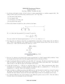


© Copyright 2026