
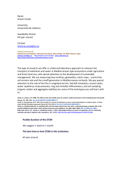
Long-Term Trends in California Mobile Source Emissions and
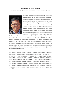
Article
pubs.acs.org/est
Long-Term Trends in California Mobile Source Emissions and
Ambient Concentrations of Black Carbon and Organic Aerosol
Brian C. McDonald†
Department of Civil & Environmental Engineering, University of California, Berkeley, Berkeley, California 94720-1710, United States
Allen H. Goldstein
Department of Environmental Science, Policy, & Management, University of California, Berkeley, Berkeley, California 94720-3140,
United States
Robert A. Harley*
Department of Civil & Environmental Engineering, University of California, Berkeley, Berkeley, California 94720-1710, United States
S Supporting Information
*
ABSTRACT: A fuel-based approach is used to assess long-term trends (1970−2010)
in mobile source emissions of black carbon (BC) and organic aerosol (OA, including
both primary emissions and secondary formation). The main focus of this analysis is the
Los Angeles Basin, where a long record of measurements is available to infer trends in
ambient concentrations of BC and organic carbon (OC), with OC used here as a proxy
for OA. Mobile source emissions and ambient concentrations have decreased similarly,
reflecting the importance of on- and off-road engines as sources of BC and OA in urban
areas. In 1970, the on-road sector accounted for ∼90% of total mobile source emissions
of BC and OA (primary + secondary). Over time, as on-road engine emissions have
been controlled, the relative importance of off-road sources has grown. By 2010, offroad engines were estimated to account for 37 ± 20% and 45 ± 16% of total mobile
source contributions to BC and OA, respectively, in the Los Angeles area. This study
highlights both the success of efforts to control on-road emission sources, and the
importance of considering off-road engine and other VOC source contributions when
assessing long-term emission and ambient air quality trends.
■
INTRODUCTION
Two major constituents of airborne fine particulate matter are
black carbon (BC) and organic aerosol (OA). Bond et al.1
report BC as the second largest contributor to anthropogenic
climate forcing after carbon dioxide globally. In North America,
the two largest sources of BC are on-road and off-road diesel
engines, which together accounted for about half of total BC
emissions in the year 2000.1 Because BC is abundant in diesel
particulate matter emissions,2 BC is sometimes used as a tracer
for diesel sources.3 BC present in diesel exhaust provides solid
particle surface area upon which other compounds may
condense or adsorb, including volatile, semivolatile, and lowvolatility organics.4 Diesel exhaust has been classified as a
known human carcinogen by the International Agency for
Research on Cancer. Short-term exposure to diesel exhaust has
been associated with impaired vascular function.5−7
OA has been found to comprise a major fraction of
submicrometer airborne particle mass at urban and rural/
remote measurement sites around the world.8,9 OA exerts a
negative radiative forcing that affects global climate.10 Unlike
BC, which is emitted directly from sources into the atmosphere,
© 2015 American Chemical Society
OA arises due to both direct emissions of primary organic
aerosol (POA) as well as in situ atmospheric formation of
secondary organic aerosol (SOA) from volatile or semivolatile
organic precursors. Many of these organics can be oxidized in
the atmosphere to form condensable low-volatility products.9,11
Over time, there has been increasing recognition of the
importance of SOA relative to POA. High relative abundances
of SOA were reported in the Los Angeles area as early as
1973,12 and SOA is thought to be especially dominant during
summertime air pollution episodes.13−15 Other studies have
found POA to dominate over SOA during less polluted time
periods15,16 and during wintertime.17 Recent studies8,9,18−20
have generally concluded that SOA is the dominant
contributor, responsible for about two-thirds of submicrometer
OA mass in urban areas around the world, and for even higher
fractions of OA in downwind/remote locations.
Received:
Revised:
Accepted:
Published:
5178
December
March 16,
March 20,
March 20,
4, 2014
2015
2015
2015
DOI: 10.1021/es505912b
Environ. Sci. Technol. 2015, 49, 5178−5188
Article
Environmental Science & Technology
Another area of debate has been the relative importance of
gasoline versus diesel engine sources of POA emissions.
Schauer et al.16 found diesel exhaust emissions dominated the
on-road contribution to POA in Los Angeles, whereas Watson
et al.21 concluded the opposite was true in Denver. There is
further debate as to the relative importance of volatile organic
compound (VOC) emissions from gasoline versus diesel
engines as precursors to formation of anthropogenic
SOA.22,23 Gentner et al.23 estimate that the fraction of VOC
emissions converted to SOA from diesel fuel-related emissions
is about 7 times greater than for gasoline engines, and found
that diesel engines are the dominant source of vehicular SOA in
Los Angeles. In contrast, Bahreini et al.22 found that gasoline
vehicles dominated SOA formation in Los Angeles during the
Calnex field study in 2010. Recent laboratory measurements
suggest that SOA production from passenger vehicle exhaust
VOC emissions is higher than aerosol yields calculated based
on the composition of unburned gasoline.24,25 Major questions
also remain about whether SOA formation from VOC emitted
by motor vehicles and other sources have been underestimated
in smog chamber studies as compared to real atmospheric
conditions.26,27
The objectives of this study are to describe long-term trends
in (1) ambient BC and organic carbon (OC) concentrations,
and (2) mobile source emissions relevant to the abundances of
primary and secondary carbonaceous aerosols. Mobile sources
include on-road and off-road engines, both gasoline and diesel
powered. Emissions and ambient trends are compared to
reconcile observed changes in atmospheric concentrations with
long-term emission trends. The present study examines the
historical record of ambient BC and OC concentrations for the
Los Angeles area, using data from both special field studies and
routine monitoring, spanning a time period of more than 4
decades. A complementary analysis of long-term trends in
emissions and ambient concentrations of BC is also presented
for the San Francisco Bay Area. A national ambient air quality
standard for fine particulate matter (PM2.5) was first established
in the U.S. in 1997, and the resulting record of ambient air
monitoring data is still relatively short (∼15 years). Other
studies reporting long-term trends in carbonaceous aerosols28−31 have typically focused on BC, though some studies
also include trends for OC.32
Figure 1. Long-term trends in fuel use by mobile sources in California.
All sources shown here use gasoline or diesel fuel, except for large
ocean-going vessels, which burn residual fuel oil. Residual fuel that is
consumed in international waters has been excluded. Also, farm
equipment emissions occur predominantly in rural areas, so
agricultural use of diesel fuel is not shown. Fuel use by heavy
equipment is broken down into military, commercial/industrial (Com
& Ind), and construction sectors. The secondary y-axis indicates a
separate scale for on-road use of gasoline, which dominates liquid fuel
sales in California.
construction and farm equipment, railroad locomotives, marine
vessels such as fishing boats, tugboats and ferries, and other
commercial and industrial engines. Also shown is heavy residual
fuel oil consumed by ocean-going marine vessels. Results from
surveys of distillate fuel wholesalers conducted by the U.S.
Energy Information Administration (EIA) that resolve fuel sales
by end use sector were used to define activity by off-road
engine type;35 this dataset has been available since 1984. Based
on previous work by Kean et al.36 we excluded distillate fuel
sales intended for use in furnaces, boilers, and for electric power
generation, where combustion air and fuel are typically
premixed, and resulting particle emissions are much lower
than for diesel engines. Prior to 1984, trends in off-road engine
activity were estimated using economic sector data37,38 and the
EIA’s State Energy Data System39 (Figures S1 and S2,
Supporting Information). We considered carefully which
proxies best replicated trends in off-road engine activity;
more details are presented in the Supporting Information.
Estimates of fuel use in off-road gasoline engines are taken
from California’s OFFROAD model.40 Off-road gasoline
engines include lawnmowers, hedge trimmers, leaf blowers,
small generators, recreational vehicles and watercraft, and other
two- and four-stroke engines.
On-Road Diesel Engine Emission Factors. Emission
factors for exhaust particulate matter (PM), expressed in units
of grams of pollutant emitted per kg of diesel fuel burned, are
derived from on-road measurements. Table S3 (Supporting
Information) provides details on the data sources used for this
analysis, which include measurements at the Tuscarora and
Allegheny Mountain Tunnels in Pennsylvania,41,42 and the
Caldecott Tunnel in Oakland.43−49 Additional measurements
have been made in roadway tunnels in Baltimore,41 Houston,50
and Pittsburgh.51 Only the Tuscarora (1976−1999) and
Caldecott (1996−2010) tunnels have long-term measurements.
We account for engine load differences between these two
tunnels, which leads to a steeper rate of decrease in exhaust PM
■
MATERIALS AND METHODS
Fuel Sales Data. We use taxable sales of gasoline and diesel
fuel as measures of passenger vehicle and diesel truck activity,
respectively. In the U.S., on-road consumption of diesel fuel
occurs primarily in the engines of medium- and heavy-duty
trucks rather than in passenger vehicles. Diesel fuel sales for use
in off-road engines are exempt from excise taxes and are tracked
separately from fuel sales for on-road engines. For the period
from 1990 to 2010, we use available estimates of on-road
gasoline and diesel fuel consumption for the Los Angeles Basin
reported by McDonald et al.,33 and apply the same approach to
estimate fuel consumption in the San Francisco Bay Area. To
extend gasoline and diesel engine emission trends further back
in time (Figure 1), ratios of fuel sales in earlier years relative to
1990 were estimated from state-level fuel sales reports.34 These
ratios were then used to extrapolate back in time based on
gasoline and diesel fuel use as of 1990 for the two air basins of
interest here (Tables S1 and S2, Supporting Information).
Separate estimates of fuel use by off-road diesel engines are
also shown in Figure 1. Off-road uses of diesel fuel include
5179
DOI: 10.1021/es505912b
Environ. Sci. Technol. 2015, 49, 5178−5188
Article
Environmental Science & Technology
emission factors over time, as compared to a simple regression
across all tunnel observations (Table S4, Supporting
Information).
Other pollutants (BC, OC, and total VOC emissions) from
heavy-duty trucks are estimated by ratio to PM, using results
from tunnel studies (Table S3, Supporting Information) and
chassis dynamometer emissions testing (Table S5, Supporting
Information).52−56 All three pollutants are well correlated with
PM (R2 > 0.70, see Figures S3−S5, Supporting Information).
An OA/OC ratio of 1.25, appropriate for hydrocarbon-like
POA emissions, is used to convert OC to POA mass57 for all
mobile sources considered in this study.
On-Road Gasoline Engine Emission Factors. Light-duty
vehicle emissions of PM, BC, OC, and total VOC are estimated
by ratio to carbon monoxide (CO). McDonald et al.58 have
reviewed and compiled CO emission factor data from roadway
tunnel and roadside emission spectrometer (“remote sensing”)
studies conducted between 1990 and 2010. A regression
analysis of additional tunnel studies (Table S6, Supporting
Information) and McDonald et al.58 was used to characterize
changes in fleet-averaged CO emission factors between 1970
and 2010 (see Table S7, Supporting Information, and Figure
2b).
Estimates of excess emissions associated with cold engine
starting are included based on predictions from the EMFAC
model,59 which predicts increasing start-related contributions to
tailpipe emissions over time, from 16% in 1990 to 26% in 2010.
A similar trend is assumed prior to 1990. Early vehicle fleets
included high fractions of automobiles not equipped with
catalysts, which would not contribute to cold start emissions.
Emission ratios of other pollutants to CO were derived from
on-road emission studies (Table S6, Supporting Information)
and based on results of laboratory emission testing (Table S8,
Supporting Information).55,60−63 Engines tested span a range of
model years from 1965 to 2012. Both VOC (Figure S6,
Supporting Information) and PM (Figure S7, Supporting
Information) are well correlated with CO, with similarly large
decreases in emission factors of all three pollutants over time.
Particle emissions from gasoline engine exhaust are mostly
carbonaceous, with OC being the dominant fraction. Both OC
and BC are well correlated with total exhaust PM emissions
(Figure S8, Supporting Information). Over time, the relative
abundance of BC in PM has been increasing, as PM emission
factors have been decreasing. Rogge et al.61 found noncatalyst
vehicles emitted much higher amounts of OC relative to BC, as
compared to catalyst-equipped vehicles.
Off-Road Engine Emission Factors. PM emission factors
from Dallmann et al.64 are used for off-road heavy-equipment,
marine vessels, and locomotives. To estimate carbonaceous
aerosol components from overall PM, we use OC/PM and BC/
PM mass fractions from Chow et al.65 specific to each off-road
sector (see Tables S9 and S10, Supporting Information). We
note that PM emission factors for off-road heavy diesel
equipment tend to be significantly higher than for heavy-duty
trucks when emissions are expressed on a per unit of fuel
burned basis, and hence off-road engines can be an important
source of particle emissions even at relatively low fuel
consumption levels. To estimate VOC emissions from offroad diesel engines, we assume the same VOC/PM ratio as for
on-road diesel engines. Off-road gasoline emission factors of
primary OC and VOC are taken from laboratory tests,66−68
reported on mass of fuel burned basis, separately for two- and
four-stroke engines (Table S11, Supporting Information). More
Figure 2. (a) Trends in heavy-duty diesel (blue) running exhaust
emission factors for PM derived from regression analysis of tunnel
studies. Early Tuscarora and Allegheny Mountain tunnel measurements are shown for comparison (dark band at left). Three fleetaveraged PM emission factors for selected calendar years (open
squares) from chassis dynamometer emission tests are shown, but
were not included in the regression. Plotted against the right axis are
measured PM concentrations in a mixed-traffic bore of the Caldecott
Tunnel (red diamonds). Shaded bands show 95% confidence interval
for the regression. (b) Trends in light-duty gasoline running exhaust
emission factors for CO derived from all on-road emission studies
(green circles). Cold start emissions are not included. Emission factor
for an uncontrolled precatalyst vehicle is shown for comparison as the
dashed line. Shaded bands show 95% confidence interval for the
regression.
details on methods and uncertainties can be found in the
Supporting Information.
SOA Yields. We merge SOA yields for emissions of
unburned gasoline and diesel fuel with laboratory measurements of tailpipe exhaust, on the basis of μg SOA μg VOC
reacted−1, where VOC reacted refers to all gas-phase organic
emissions from tailpipe exhaust (Table S12, Supporting
Information). The calculated SOA yields are then combined
with corresponding VOC emissions to estimate contributions
to SOA formation. For gasoline vehicles, we use aerosol yields
reported by Gentner et al.,23 Gordon et al.,24 and Jathar et al.25
Between 1995 and 1996, gasoline was reformulated to reduce
content of heavy/aromatic hydrocarbons in California.69 For
years prior to 1996, we recalculated bulk SOA yields following
Gentner et al.,23 using different fuel speciation profiles.69 The
result was an aerosol mass yield for pre-1996 conditions that
was 60% higher than for reformulated gasoline. Aerosol yields
in Gentner et al.23 are for individual hydrocarbons derived from
laboratory chamber studies, and overall yields were calculated
assuming SOA formation was due to emissions of unburned
fuel under high nitrogen oxide (NOx) conditions. The yields
5180
DOI: 10.1021/es505912b
Environ. Sci. Technol. 2015, 49, 5178−5188
Article
Environmental Science & Technology
SOA assuming an aerosol yield of 0.50 μg SOA μg SVOC
reacted−1 from Zhao et al.,78 as determined in the Los Angeles
area during Calnex in 2010. We assume SOA yields for
evaporated POA change similarly to those for unburned
gasoline and diesel fuel over time with respect to decreases in
ambient OA concentrations.
Ambient BC and OC Concentrations. Ambient trends in
BC are estimated for both Los Angeles and the San Francisco
Bay Area. In the Bay Area, routine measurements of the
coefficient of haze for ambient air are available from 1967 to
2003, and these measurements are closely related and can be
converted to BC.30 In Los Angeles, a combination of
reflectance-tape based samplers31 and filter samples are used
to estimate BC concentrations. Filter data are also used to
estimate ambient OC for Los Angeles only.
Table S15 (Supporting Information) summarizes filter-based
datasets used to describe ambient carbon particle concentrations (cutpoint diameter = 2.1 or 2.5 μm depending on the
study) in the Los Angeles area. Data sources include a series of
yearlong field studies by Cass and co-workers,32,79,80 more
recent studies by the South Coast Air Quality Management
District,81,82 and routine monitoring data from the Speciation
Trends Network (STN) and National Air Surveillance
Network.83 These studies used filters to measure PM mass,
BC, and OC. Filter samples were typically collected over 24 h
time periods and subsequently analyzed in a central laboratory.
Thermal optical analysis techniques were used to differentiate
and quantify black and organic carbon contributions to total
carbon mass on each filter.
In Los Angeles, average BC concentrations from 1960 to
1982 are derived from reflectance-based tape samplers that
operated at seven locations measured across the basin. The tape
samplers were shown to be well-correlated with BC.31 From
1993 to 2010, a linear regression is performed on filter samples
described in Table S15 (Supporting Information). In the
intervening years, ambient BC concentrations are interpolated,
as discussed below in the section on BC Trends. To derive
ambient OC concentrations, correlations between filter-based
measurements of OC and BC were developed, and more
extensive records of measured BC concentrations were thereby
used to estimate OC. The similarity of slopes inferred from
regression analyses involving OC and BC measured in multiple
studies (Figure S9, Supporting Information) implies similar
long-term trends in ambient BC and OC concentrations.
A key reason why we infer OC from measured BC
concentrations is that there is a potentially large OC sampling
artifact due to adsorption of gas-phase organics onto quartz
filters, which can lead to systematic biases of up to +50%.84−86
A negative sampling artifact due to volatilization of particlephase organics collected on the filter sample is also possible,
and can occur when there is a large pressure drop over the
filter.85 Turpin et al.87 concluded that the dominant sampling
artifact in the Los Angeles Basin was due to adsorption of gasphase organics. Adsorbed carbon is often estimated by
difference between a front and back-up filter, using either
quartz-behind-quartz (QBQ) or quartz-behind-Teflon (QBT)
filter configurations. However, measurements of OC are not
always adjusted to account for sampling artifacts. For
measurements that are not corrected, face velocity (air flow
rate divided by filter cross-sectional area) is known to influence
OC measurements. At higher face velocity, the importance of
the OC adsorption artifact tends to be reduced.87 For three
studies where organic carbon was not corrected using back-up
are representative of the first several generations of oxidation
products (∼6 h of processing), and are expected to underestimate contributions to ambient SOA, especially in aged air
masses.23
Aerosol yields are also affected by environmental factors. An
important factor that we take into account is the effect of
decreasing OA concentrations in the Los Angeles atmosphere
over time, which reduces partitioning of semivolatile organics to
the particle-phase. We use an SOA parametrization described
by Jathar et al.25 to quantify the effect of changing OA
concentrations on both gasoline and diesel yields of SOA. The
yields are predicted to be 1.5 and 2 times higher, respectively, in
1970 relative to 2010. Another environmental factor that could
also lead to lower aerosol yields with time, are decreasing levels
of VOC/NOx.70,71 In the Los Angeles Basin, the VOC/NOx
ratio has fallen significantly over the past few decades.58,72
Changes in VOC/NOx ratios are not accounted for in this
analysis.
Another consideration is the increased production efficiency
of SOA per amount of VOC emitted from modern passenger
vehicles.24 Old vehicles that predate California’s Low-Emitting
Vehicle (LEV-I) emission standard, have aerosol yields that can
be well-described based on the composition of unburned
gasoline. However, automobiles designed to meet LEV-I and
LEV-II standards produce higher SOA than would be expected,
despite substantially lower total VOC emissions. These vehicles
have significant fractions of intermediate volatility organics, that
are unresolved by standard gas chromatography techniques,
and which have a high potential to form SOA in the
atmosphere once emitted.73 Following the introduction of
LEV-I vehicles, we calculate aerosol yields based on tailpipe
exhaust rather than unburned fuel for the whole vehicle fleet in
calendar years 1994 and later, similar to Ensberg et al.26 The
result is an SOA yield that is ∼3 times higher in the year 2010
than from unburned gasoline reported by Gentner et al.23
For on-road and off-road diesel engines, we take a composite
average of aerosol yields reported in the literature for both
unburned fuel and diesel exhaust.23,25,74 Diesel fuel contains
much greater abundance of intermediate volatility organics than
gasoline, and these organics form SOA in higher yields
compared to the lighter and more volatile compounds present
in gasoline. Jathar et al.25 show that SOA yields for diesel
exhaust can be understood based on the composition of
unburned fuel. SOA yields for off-road gasoline engine
emissions are based on work of Gordon et al.66
Gas−Particle Partitioning of POA. A complicating factor
is that partitioning of POA between the gas and particle phases
varies depending on organic aerosol mass loadings, the extent
to which POA emissions have been diluted with ambient air,
and ambient temperature.75 In tunnel studies and in chassis
dynamometer tests, POA emission factors are biased high
because aerosol concentrations are many times higher than in
the ambient environment, and which, in turn, favors
partitioning of low volatility organics into the particle phase.
Using estimates of gasoline and diesel POA partitioning from
May et al.,76,77 we estimate that ∼30% of gasoline and diesel
POA emissions (Table S13, Supporting Information) measured
in laboratory and tunnel studies (Table S14, Supporting
Information) will evaporate upon dilution to ambient
conditions at 25 °C (see the Supporting Information for
more details). Upon oxidation, the evaporated POA, which
includes semivolatile organic compounds (SVOCs), can readily
form SOA. We estimate contributions of evaporated POA to
5181
DOI: 10.1021/es505912b
Environ. Sci. Technol. 2015, 49, 5178−5188
Article
Environmental Science & Technology
Figure 3. (a) Trends in ambient BC concentrations (right axis) for the Los Angeles area, compared with fuel-based inventory trends for BC
emissions from on-road diesel (blue) and all mobile sources (gray). The latter is the sum of on-road diesel, on-road gasoline, and off-road diesel BC
emissions. The ambient trend from 1960 to 1982 is derived from reflectance tape data (brown), and from 1993 to 2011 from filter samples listed in
Table S15 (Supporting Information). Ambient values in between are interpolated. Error bars on the ambient data show the 95% confidence interval
for basin-average concentrations, and reflect spatial variability. Shaded bands for the fuel-based inventory also represent 95% confidence intervals. (b)
Trends in mobile source emissions of BC broken down by major source category and shown as stacked area contributions to the total. (c) Same as
panel a for the San Francisco Bay Area. Trends in annual average ambient BC concentrations (right axis) derived from coefficient of haze monitoring
in the San Francisco Bay Area. Error bars show the minimum and maximum values of annually averaged BC concentrations across COH monitoring
locations. (d) Same as panel b for the San Francisco Bay Area.
filter data, and where sampling was done at low air flow rates,
the OC to BC ratio is clearly elevated compared to other
studies (Figure S9, Supporting Information). To avoid biasing
OC estimates, we derive a relationship between OC and BC
from the other studies where the adsorption artifact is already
corrected for using either QBQ or QBT paired filter
configurations, or where the adsorption artifact was mitigated
by use of high sample air flow rates.
Measurements of OC are the best available proxy for how
ambient levels of organic aerosol have changed over time.
Similar OA/OC mass ratios have been reported across various
urban areas, even though ambient OA levels vary substantially.
OA/OC ratios in Mexico City, 88 Los Angeles,19 and
Pittsburgh89 have been reported to range from 1.6 to 1.8. In
contrast, absolute OA concentrations vary by a factor of 4
across these cities.19,89,90 A reanalysis of early carbonaceous
aerosol samples collected in the Los Angeles Basin during
1982,91 found similar OA/OC ratios ranging from 1.6 to 1.8
across three urban sites.92 We use a constant OA/OC mass
ratio of 1.7 to convert ambient concentrations of OC to OA.
measurements of diesel truck emissions at a weigh station on
Interstate Highway 5 near Redding, California.93 To evaluate
the slope of the emission factor trend line, we compare
emission factor trends with results of repeated measurements of
pollutant concentrations at the Caldecott tunnel in the San
Francisco Bay Area.43−49 The evolution of measured PM
concentrations normalized to truck traffic flow at this location
(Table S14, Supporting Information) is plotted on the
secondary vertical axis of Figure 2a; the trend is a proxy for
changes in diesel truck emission factors shown on the same plot
and is consistent with our regression. Tunnel concentrations
are shown on the secondary axis because an early study by
Hering et al.47 reported PM but not carbon dioxide, which is
needed to calculate emission factors.
The first organized emission inspections for heavy-duty
trucks started in 1970 and were aimed to reduce visible smoke
under steady state engine operation.3 The first diesel exhaust
emission standards specifically for PM were implemented much
later, for 1988 and newer engines.44,53 Initial efforts to lower
diesel PM emissions involved changes to engine design to
reduce lubricating oil emissions and to improve air−fuel mixing
(thereby lowering BC emissions), rather than installing aftertreatment control technologies.3 Starting with the 2007 model
year, allowable PM emission rates for heavy-duty diesel engines
were lowered by an order of magnitude. Diesel particle filters
(DPF) are now included as standard equipment on most new
■
RESULTS AND DISCUSSION
BC Trends. Over a 40 year period between 1970 and 2010,
heavy-duty diesel truck exhaust PM emission factors decreased
by a factor of ∼7, as shown in Figure 2a. Our PM emission
factor of 0.68 ± 0.31 g kg−1 fuel as of 2010 agrees well with
5182
DOI: 10.1021/es505912b
Environ. Sci. Technol. 2015, 49, 5178−5188
Article
Environmental Science & Technology
engines, and large resulting decreases in BC emission factors
have been observed.94,95 The effects of large numbers of DPFequipped engines entering into service is not accounted for in
this analysis, so emission factor trends in Figure 2a may show a
change in slope when projected forward in time beyond ∼2010.
When evolving values of taxable diesel fuel sales and emission
factors are combined for the period 1970−2010, a resulting
trend in BC emissions can be derived, as shown in Figure 3.
The spatial domains for which emissions were estimated
include the South Coast/Los Angeles (top) and San Francisco
Bay Area (bottom) air basins. The sum of all mobile source
emissions, including on-road gasoline, on-road diesel, and offroad diesel is shown in Figure 3b,d for these air basins, and
compared with trends in ambient BC concentrations. Off-road
gasoline engines are not shown because they are a very minor
contributor to BC emissions66,68 (most of the PM emissions
from these engines consist of lubricating oil/POA rather than
BC).
A surprising result is that on-road heavy-duty diesel trucks
have never accounted for more than half of the total BC
emissions from all mobile sources (Figure 3a,c). In 1970,
passenger vehicles were of similar importance as sources of BC
emissions. In 2010, gasoline vehicles are now a relatively minor
source of BC (only 15 ± 7% of the total), and diesel trucks are
the largest contributor (48 ± 27%). However, off-road heavy
diesel engines are also a significant source of BC emissions (37
± 20%). Fuel volumes consumed by off-road diesel engines
were much less than for on-road diesel trucks as of 2010
(Figure 1). However, BC emission factors are twice as high in
off-road versus on-road diesel engines when expressed per unit
of fuel burned basis. Differences in emission factors arise from
delayed implementation of emission standards for off-road
diesel engines, which began in 1996, decades after the first
visible smoke regulations were implemented on on-road diesel
engines in 1970.3
Figure 1 shows how diesel fuel use in off-road heavy
equipment has changed over time. Between 1975 and 1980,
there was a ∼50% increase in off-road sales of diesel fuel in
California. This was followed by a similar decrease between
1987 and 1992. The large fluctuations in California off-road fuel
purchases were seen in the commercial and industrial sectors;
much less variability was seen at the national level (Figure S1,
Supporting Information). The large differences between
California and the U.S. diesel fuel sales trends likely resulted
from different limits on sulfur content in diesel fuel. The
decrease in fuel sales in California occurred when use of highsulfur diesel (fuel with over 500 ppm sulfur content used to be
allowed) was being phased-out in off-road engines, a statewide
rule that was specific to California (see Figure S1, Supporting
Information).36 BC emissions from off-road diesel engines are
shown in Figure 3b,d. Because emission standards for off-road
diesel engines had not been established yet, changes in activity
(i.e., fuel sales) were the dominant factor affecting off-road
diesel emissions prior to the mid-1990s. Reduced off-road
engine activity appears to explain, at least in part, why ambient
concentrations of BC were decreasing more rapidly around
1990, which is evident in both the Los Angeles Basin (Figure
3b) and the San Francisco Bay Area (Figure 3d). The
noticeable drop in off-road fuel purchases around 1990 is not
affected by interpolation methods used in this study for
extrapolating off-road activity in earlier years. State-level fuel
survey data are available beginning in 1984 and capture the
downturn in California off-road diesel engine activity.35
Between 1970 and 2010, overall mobile source emissions of
black carbon decreased by a factor of 2 (Figure 3). We attribute
∼70% of the decrease to on-road gasoline vehicles, and the
other ∼30% to efforts to control PM emissions from diesel
trucks. Off-road diesel emissions of BC grew rapidly and then
dropped (Figure 1). In contrast to the present study, the
presumption in the literature has been that BC decreases in
California have been driven by control of on-road diesel
emission sources.29,30
In the San Francisco Bay Area, there is good agreement
between our mobile source inventory and coefficient of hazederived BC concentrations (Figure 3c). Prior to 1970, there is a
very sharp decrease in ambient BC concentrations, possibly due
to decreased emissions from stationary sources. Ambient BC
concentrations in Los Angeles exhibit many of the same
features as the San Francisco Bay Area, but lack the sudden
drop in BC concentrations around 1970 (Figure 3a). The
ambient BC concentration trend also exhibits a slight decrease
rather than increase between 1970 and 1980. The differences
between Los Angeles and San Francisco Bay Area also may
reflect regional differences in pollution sources and/or policies
to control stationary source emissions.
After 1980, mobile sources are expected to be a dominant
contributor to BC. First, other potentially important sources of
BC, including industrial uses of coal, residential heating, and
open burning are no longer expected to be significant in
California cities.1 Second, ambient BC concentrations are
known to exhibit day-of-week cycles,30 consistent with
decreases in diesel truck activity on weekends compared to
weekdays.96 Passenger vehicles96 and stationary/residential
sources97 do not exhibit strong day-of-week cycles in activity
patterns. Lastly, the consistency of our emissions inventory
with ambient trends corroborates the importance of mobile
sources to BC.
OA Trends. The OA analysis focuses only on the Los
Angeles Basin. It is well documented that tailpipe emissions of
CO and VOC from passenger vehicles have decreased rapidly
due to widespread deployment of catalytic converters along
with supportive changes in fuel properties.58,98 Between 1970
and 2010, gasoline engine emission factors of CO were found
to decrease by 7.4% per year (Figure 2b). In 1970, our
regression estimate is in agreement with an emission factor for
precatalyst vehicles (model years 1957−1965) calculated by
Harley et al.99 After accounting for ∼60% increase in gasoline
sales, and a growing contribution to overall emissions
associated with cold engine starting, on-road gasoline engine
emissions of CO still decreased by a factor of 10 between 1970
and 2010. In this study, CO provides a baseline from which we
estimate emissions of POA and VOC, with VOC emissions, in
turn leading to the formation of SOA. All three pollutants have
trended similarly to CO, and exhibited order of magnitude
reductions between 1970 and 2010. Estimates of SOA
production from gasoline emissions account for effects of
decreasing aerosol mass loadings in the atmosphere, decreased
aromatic content of gasoline, and higher SOA produced per
unit mass of VOC emitted from newer vehicles.
It is of interest to reconcile changes in emissions of VOC and
POA with long-term trends in ambient concentrations of
organic aerosol. As described above, we infer ambient OC
concentrations in the Los Angeles Basin using relationships
shown in Figure S9 (Supporting Information) combined with
measured BC concentrations, and then multiply OC in all cases
by an OA/OC mass ratio of 1.7.19 Our analysis indicates that
5183
DOI: 10.1021/es505912b
Environ. Sci. Technol. 2015, 49, 5178−5188
Article
Environmental Science & Technology
of catalytic converters to treat on-road gasoline exhaust, with
resulting large reductions in VOC emissions that lead to SOA
formation. Exhaust after-treatment devices have not been
widely used in other mobile source sectors until recently.
Emissions are broken down by on-road and off-road engine,
fuel categories, and by POA and SOA separately in Figure 4b.
As of 1970, on-road gasoline engines accounted for 82 ± 32%
of mobile source contributions to OA (POA + SOA), and
clearly dominated over all other mobile source contributions.
By 2010, on-road gasoline engines accounted for 43 ± 16% of
the mobile source contribution to OA, followed by off-road
diesel and gasoline equipment accounting for ∼20% each. Offroad gasoline equipment are increasingly becoming an
important source of precursor emissions to ozone and SOA.
Platt et al.101 suggest that in many cities around the globe, twostroke scooters are the largest source of vehicular PM and SOA.
We estimate that VOC emission factors on a fuel basis are 170
± 40 times higher in off-road gasoline engines (e.g., lawn and
garden equipment) than for the 2010 on-road light-duty vehicle
fleet. As control of on-road pollution sources was an early focus
of air quality management efforts, other sources of POA and
SOA-forming emissions are likely to have grown in relative
importance over time.
As shown in Figure 4a, mobile source contributions to OA
(including both primary and secondary sources) and
constructed OA concentrations show similar long-term downward trends. The similarity between mobile source emissions
and the ambient OA trends reflects the historical importance of
on-road and off-road engines as air pollution sources in the Los
Angeles Basin. Note that the two independent vertical axes of
Figure 4b are aligned in a similar manner as in Figure 3. The
relative scaling of the axes aligns primary pollutant emissions
with resulting ambient concentrations (1 μg m−3 corresponds
to 4−5 tons per day of primary emissions under annual average
conditions). The lack of a gap between emissions and ambient
trend lines in Figure 4b suggests that our inventory-based
approach applying SOA yields to gasoline and diesel VOC
emissions is giving reasonable results.
There are also other potentially important stationary and
area source emissions, which we have not considered in this
analysis, but may also be making noteworthy contributions to
OA. These other sources of OA include cooking, wood smoke
and forest fires, as well as SOA due to biogenic VOC
emissions.13,16,17,19,20 Zotter et al.102 suggest that 58 ± 15% of
OC measured at Pasadena during CalNex in 2010 was
nonfossil. Including these other sources of organic aerosol
would be likely to flatten the overall OA emissions trend, and
bring it into better agreement with the ambient OA
concentration trend.
In summary, we found consistent pictures of long-term
trends in mobile source emissions of carbon particles and
corresponding ambient concentrations for two major urban
areas in California. This suggests that mobile sources in the past
have dominated contributions to carbonaceous aerosols
(including primary emissions plus secondary formation). As
of 1970, mobile source emissions were dominated by on-road
sources for both BC and OA (∼90%). By 2010, off-road
engines accounted for 37 ± 20% and 45 ± 16% of mobile
source-related BC and OA, respectively. Emission uncertainties
for individual mobile source categories are summarized in Table
S16 (Supporting Information). For the urban areas considered
in this study, it appears to be increasingly important that air
quality management plans consider and address the air
the constructed OA concentrations in the Los Angeles Basin
decreased from 15.5 ± 2.7 μg m−3 in 1970 to 5.1 ± 1.4 μg m−3
in 2010 (Figure 4).
Figure 4. (a) Trends in ambient organic aerosol concentrations (right
axis) inferred from filter samples for the Los Angeles area, compared
with estimated emission contributions to OA from on-road gasoline
vehicles (green) and from all mobile sources (gray). Total OA
emissions are calculated as the sum of both primary and secondary
contributions. SOA-forming emissions equals gas-phase VOC and
evaporated semivolatile POA emissions, multiplied by an aerosol yield
for each (see text). Shaded bands for the emissions inventory represent
a 95% confidence interval. Ambient OA values are scaled from OC
measurements that are shown as reported (closed circles) or estimated
using OC to BC relationships derived in Figure S9 (Supporting
Information) (open circles). Error bars for ambient organic aerosol
denote 95% confidence intervals for basin-average concentrations, and
reflect spatial variability. Note the logarithmic scale. (b) Trend in
mobile source emissions of OA as in the top panel, broken down by
major source category and plotted on a linear scale.
Estimated on-road and off-road contributions to OA
(including both primary and secondary sources) and ambient
OA concentrations are compared in Figure 4a on a logarithmic
scale. The step change seen in Figure 4a for gasoline-related
SOA between 1995 and 1996 is due to a statewide program
requiring use of reformulated gasoline, which lowered the
aromatic and heavy hydrocarbon content of gasoline as well as
the SOA-forming potential of related VOC emissions.100 It is
clear that on-road gasoline contributions to POA and SOA
formation are decreasing at a much faster rate than ambient
OA. When other mobile sources are included, the emissions
trend becomes flatter, with OA decreasing by a factor of 4−5
between 1970 and 2010, in agreement with the constructed
record of ambient OA concentrations. A slower rate of decrease
in OA is expected when contributions from on-road diesel and
off-road engines are included. There is now near-universal use
5184
DOI: 10.1021/es505912b
Environ. Sci. Technol. 2015, 49, 5178−5188
Article
Environmental Science & Technology
(7) Smith, K. R.; Jerrett, M.; Anderson, H. R.; Burnett, R. T.; Stone,
V.; Derwent, R.; Atkinson, R. W.; Cohen, A.; Shonkoff, S. B.; Krewski,
D.; Pope, C. A.; Thun, M. J.; Thurston, G. Health and climate change.
5 Public health benefits of strategies to reduce greenhouse-gas
emissions: Health implications of short-lived greenhouse pollutants.
Lancet 2009, 374, 2091−2103 DOI: 10.1016/S0140-6736(09)617165.
(8) Zhang, Q.; Jimenez, J. L.; Canagaratna, M. R.; Allan, J. D.; Coe,
H.; Ulbrich, I.; Alfarra, M. R.; Takami, A.; Middlebrook, A. M.; Sun, Y.
L.; Dzepina, K.; Dunlea, E.; Docherty, K.; DeCarlo, P. F.; Salcedo, D.;
Onasch, T.; Jayne, J. T.; Miyoshi, T.; Shimono, A.; Hatakeyama, S.;
Takegawa, N.; Kondo, Y.; Schneider, J.; Drewnick, F.; Borrmann, S.;
Weimer, S.; Demerjian, K.; Williams, P.; Bower, K.; Bahreini, R.;
Cottrell, L.; Griffin, R. J.; Rautiainen, J.; Sun, J. Y.; Zhang, Y. M.;
Worsnop, D. R. Ubiquity and dominance of oxygenated species in
organic aerosols in anthropogenically-influenced Northern Hemisphere midlatitudes. Geophys. Res. Lett. 2007, 34, Article No. L13801,
DOI: 10.1029/2007gl029979.
(9) Jimenez, J. L.; Canagaratna, M. R.; Donahue, N. M.; Prevot, A. S.
H.; Zhang, Q.; Kroll, J. H.; DeCarlo, P. F.; Allan, J. D.; Coe, H.; Ng, N.
L.; Aiken, A. C.; Docherty, K. S.; Ulbrich, I. M.; Grieshop, A. P.;
Robinson, A. L.; Duplissy, J.; Smith, J. D.; Wilson, K. R.; Lanz, V. A.;
Hueglin, C.; Sun, Y. L.; Tian, J.; Laaksonen, A.; Raatikainen, T.;
Rautiainen, J.; Vaattovaara, P.; Ehn, M.; Kulmala, M.; Tomlinson, J.
M.; Collins, D. R.; Cubison, M. J.; Dunlea, E. J.; Huffman, J. A.;
Onasch, T. B.; Alfarra, M. R.; Williams, P. I.; Bower, K.; Kondo, Y.;
Schneider, J.; Drewnick, F.; Borrmann, S.; Weimer, S.; Demerjian, K.;
Salcedo, D.; Cottrell, L.; Griffin, R.; Takami, A.; Miyoshi, T.;
Hatakeyama, S.; Shimono, A.; Sun, J. Y.; Zhang, Y. M.; Dzepina, K.;
Kimmel, J. R.; Sueper, D.; Jayne, J. T.; Herndon, S. C.; Trimborn, A.
M.; Williams, L. R.; Wood, E. C.; Middlebrook, A. M.; Kolb, C. E.;
Baltensperger, U.; Worsnop, D. R. Evolution of organic aerosols in the
atmosphere. Science 2009, 326, 1525−1529 DOI: 10.1126/science.1180353.
(10) IPCC. Climate Change 2013: the Physical Science Basis.
Contribution of Working Group I to the Fifth Assessment Report of the
Intergovernmental Panel on Climate Change; Intergovernmental Panel
on Climate Change: Cambridge, U. K. and New York, NY, 2013.
http://www.ipcc.ch/report/ar5/wg1/ (accessed November 21, 2014).
(11) Goldstein, A. H.; Galbally, I. E. Known and unexplored organic
constituents in the earth’s atmosphere. Environ. Sci. Technol. 2007, 41,
1514−1521 DOI: 10.1021/Es072476p.
(12) Appel, B. R.; Colodny, P.; Wesolowski, J. J. Analysis of
carbonaceous materials in Southern California atmospheric aerosols.
Environ. Sci. Technol. 1976, 10, 359−363 DOI: 10.1021/Es60115a005.
(13) Schauer, J. J.; Fraser, M. P.; Cass, G. R.; Simoneit, B. R. T.
Source reconciliation of atmospheric gas-phase and particle-phase
pollutants during a severe photochemical smog episode. Environ. Sci.
Technol. 2002, 36, 3806−3814 DOI: 10.1021/Es011458j.
(14) Turpin, B. J.; Huntzicker, J. J. Secondary formation of organic
aerosol in the Los Angeles Basin: A descriptive analysis of organic and
elemental carbon concentrations. Atmos. Environ., Part A 1991, 25,
207−215 DOI: 10.1016/0960-1686(91)90291-E.
(15) Turpin, B. J.; Huntzicker, J. J. Identification of secondary organic
aerosol episodes and quantitation of primary and secondary organic
aerosol concentrations during SCAQS. Atmos. Environ. 1995, 29,
3527−3544 DOI: 10.1016/1352-2310(94)00276-Q.
(16) Schauer, J. J.; Rogge, W. F.; Hildemann, L. M.; Mazurek, M. A.;
Cass, G. R.; Simoneit, B. R. T. Source apportionment of airborne
particulate matter using organic compounds as tracers. Atmos. Environ.
1996, 30, 3837−3855 DOI: 10.1016/1352-2310(96)00085-4.
(17) Heo, J. B.; Dulger, M.; Olson, M. R.; McGinnis, J. E.; Shelton, B.
R.; Matsunaga, A.; Sioutas, C.; Schauer, J. J. Source apportionments of
PM2.5 organic carbon using molecular marker Positive Matrix
Factorization and comparison of results from different receptor
models. Atmos. Environ. 2013, 73, 51−61 DOI: 10.1016/j.atmosenv.2013.03.004.
(18) Docherty, K. S.; Stone, E. A.; Ulbrich, I. M.; DeCarlo, P. F.;
Snyder, D. C.; Schauer, J. J.; Peltier, R. E.; Weber, R. J.; Murphy, S. M.;
pollution burdens associated with off-road engines and other
possible sources of VOCs with high SOA formation potential,
in addition to regulating emissions from on-road motor
vehicles.
■
ASSOCIATED CONTENT
S Supporting Information
*
Supplementary tables (S1−S16) and figures (S1−S9) as
referenced in the text. This material is available free of charge
via the Internet at http://pubs.acs.org/.
■
AUTHOR INFORMATION
Corresponding Author
*R. A. Harley. Tel.: (510) 643-9168. Fax: (510) 643-5264. Email: [email protected].
Present Address
†
University of Colorado, Boulder Cooperative Institute for
Research in Environmental Sciences Boulder, CO 80309-0216.
Tel.: 303-497-5094. E-mail: [email protected].
Notes
The authors declare no competing financial interest.
■
ACKNOWLEDGMENTS
This research was supported by the University of California
Multi-Campus Research Program in Sustainable Transportation. The authors thank Thomas Kirchstetter for providing
coefficient of haze data used in this analysis. The authors also
thank William Nazaroff, Drew Gentner, Dave Worton, Ravan
Ahmadov, Timothy Gordon, Joost de Gouw, and Gary Bishop
for helpful feedback.
■
REFERENCES
(1) Bond, T. C.; Doherty, S. J.; Fahey, D. W.; Forster, P. M.;
Berntsen, T.; DeAngelo, B. J.; Flanner, M. G.; Ghan, S.; Karcher, B.;
Koch, D.; Kinne, S.; Kondo, Y.; Quinn, P. K.; Sarofim, M. C.; Schultz,
M. G.; Schulz, M.; Venkataraman, C.; Zhang, H.; Zhang, S.; Bellouin,
N.; Guttikunda, S. K.; Hopke, P. K.; Jacobson, M. Z.; Kaiser, J. W.;
Klimont, Z.; Lohmann, U.; Schwarz, J. P.; Shindell, D.; Storelvmo, T.;
Warren, S. G.; Zender, C. S. Bounding the role of black carbon in the
climate system: A scientific assessment. J. Geophys. Res.: Atmos. 2013,
118, 5380−5552 DOI: 10.1002/Jgrd.50171.
(2) Watson, J. G.; Chow, J. C.; Lowenthal, D. H.; Pritchett, L. C.;
Frazier, C. A.; Neuroth, G. R.; Robbins, R. Differences in the carbon
composition of source profiles for diesel-powered and gasolinepowered vehicles. Atmos. Environ. 1994, 28, 2493−2505
DOI: 10.1016/1352-2310(94)90400-6.
(3) Lloyd, A. C.; Cackette, T. A. Diesel engines: Environmental
impact and control. J. Air Waste Manage. 2001, 51, 809−847
DOI: 10.1080/10473289.2001.10464315.
(4) Ristovski, Z. D.; Miljevic, B.; Surawski, N. C.; Morawska, L.;
Fong, K. M.; Goh, F.; Yang, I. A. Respiratory health effects of diesel
particulate matter. Respirology 2012, 17, 201−212 DOI: 10.1111/
j.1440-1843.2011.02109.x.
(5) Barath, S.; Mills, N. L.; Lundback, M.; Tornqvist, H.; Lucking, A.
J.; Langrish, J. P.; Soderberg, S.; Boman, C.; Westerholm, R.; Londahl,
J.; Donaldson, K.; Mudway, I. S.; Sandstrom, T.; Newby, D. E.;
Blomberg, A. Impaired vascular function after exposure to diesel
exhaust generated at urban transient running conditions. Part Fibre
Toxicol. 2010, 7, Article No. 19, DOI: 10.1186/1743-8977-7-19.
(6) Mills, N. L.; Tornqvist, H.; Gonzalez, M. C.; Vink, E.; Robinson,
S. D.; Soderberg, S.; Boon, N. A.; Donaldson, K.; Sandstrom, T.;
Blomberg, A.; Newby, D. E. Ischemic and thrombotic effects of dilute
diesel-exhaust inhalation in men with coronary heart disease. New Engl.
J. Med. 2007, 357, 1075−1082 DOI: 10.1056/Nejmoa066314.
5185
DOI: 10.1021/es505912b
Environ. Sci. Technol. 2015, 49, 5178−5188
Article
Environmental Science & Technology
Seinfeld, J. H.; Grover, B. D.; Eatough, D. J.; Jimenez, J. L.
Apportionment of primary and secondary organic aerosols in Southern
California during the 2005 study of organic aerosols in Riverside
(SOAR-1). Environ. Sci. Technol. 2008, 42, 7655−7662 DOI: 10.1021/
Es8008166.
(19) Hayes, P. L.; Ortega, A. M.; Cubison, M. J.; Froyd, K. D.; Zhao,
Y.; Cliff, S. S.; Hu, W. W.; Toohey, D. W.; Flynn, J. H.; Lefer, B. L.;
Grossberg, N.; Alvarez, S.; Rappenglueck, B.; Taylor, J. W.; Allan, J. D.;
Holloway, J. S.; Gilman, J. B.; Kuster, W. C.; De Gouw, J. A.; Massoli,
P.; Zhang, X.; Liu, J.; Weber, R. J.; Corrigan, A. L.; Russell, L. M.;
Isaacman, G.; Worton, D. R.; Kreisberg, N. M.; Goldstein, A. H.;
Thalman, R.; Waxman, E. M.; Volkamer, R.; Lin, Y. H.; Surratt, J. D.;
Kleindienst, T. E.; Offenberg, J. H.; Dusanter, S.; Griffith, S.; Stevens,
P. S.; Brioude, J.; Angevine, W. M.; Jimenez, J. L. Organic aerosol
composition and sources in Pasadena, California, during the 2010
CalNex campaign. J. Geophys. Res.: Atmos. 2013, 118, 9233−9257
DOI: 10.1002/Jgrd.50530.
(20) Williams, B. J.; Goldstein, A. H.; Kreisberg, N. M.; Hering, S. V.;
Worsnop, D. R.; Ulbrich, I. M.; Docherty, K. S.; Jimenez, J. L. Major
components of atmospheric organic aerosol in Southern California as
determined by hourly measurements of source marker compounds.
Atmos. Chem. Phys. 2010, 10, 11577−11603 DOI: 10.5194/acp-1011577-2010.
(21) Watson, J. G.; Fujita, E. M.; Chow, J. C.; Zielinska, B. Northern
Front Range Air Quality Study Final Report; Colorado State University:
Fort Collins, CO, 1998. http://www.dri.edu/images/stories/editors/
eafeditor/Watsonetal1998NFRAQSFinal.pdf (accessed November 21,
2014).
(22) Bahreini, R.; Middlebrook, A. M.; de Gouw, J. A.; Warneke, C.;
Trainer, M.; Brock, C. A.; Stark, H.; Brown, S. S.; Dube, W. P.;
Gilman, J. B.; Hall, K.; Holloway, J. S.; Kuster, W. C.; Perring, A. E.;
Prevot, A. S. H.; Schwarz, J. P.; Spackman, J. R.; Szidat, S.; Wagner, N.
L.; Weber, R. J.; Zotter, P.; Parrish, D. D. Gasoline emissions dominate
over diesel in formation of secondary organic aerosol mass. Geophys.
Res. Lett. 2012, 39, Article No. L06805, DOI: 10.1029/2011gl050718.
(23) Gentner, D. R.; Isaacman, G.; Worton, D. R.; Chan, A. W.;
Dallmann, T. R.; Davis, L.; Liu, S.; Day, D. A.; Russell, L. M.; Wilson,
K. R.; Weber, R.; Guha, A.; Harley, R. A.; Goldstein, A. H. Elucidating
secondary organic aerosol from diesel and gasoline vehicles through
detailed characterization of organic carbon emissions. Proc. Natl. Acad.
Sci. U. S. A. 2012, 109, 18318−18323 DOI: 10.1073/
pnas.1212272109.
(24) Gordon, T. D.; Presto, A. A.; May, A. A.; Nguyen, N. T.; Lipsky,
E. M.; Donahue, N. M.; Gutierrez, A.; Zhang, M.; Maddox, C.; Rieger,
P.; Chattopadhyay, S.; Maldonado, H.; Maricq, M. M.; Robinson, A. L.
Secondary organic aerosol formation exceeds primary particulate
matter emissions for light-duty gasoline vehicles. Atmos. Chem. Phys.
2014, 14, 4661−4678 DOI: 10.5194/acp-14-4661-2014.
(25) Jathar, S. H.; Miracolo, M. A.; Tkacik, D. S.; Donahue, N. M.;
Adams, P. J.; Robinson, A. L. Secondary organic aerosol formation
from photo-oxidation of unburned fuel: Experimental results and
implications for aerosol formation from combustion emissions.
Environ. Sci. Technol. 2013, 47, 12886−12893 DOI: 10.1021/
Es403445q.
(26) Ensberg, J. J.; Hayes, P. L.; Jimenez, J. L.; Gilman, J. B.; Kuster,
W. C.; De Gouw, J. A.; Holloway, J. S.; Gordon, T. D.; Jathar, S.;
Robinson, A. L.; Seinfeld, J. H. Emission factor ratios, SOA mass
yields, and the impact of vehicular emissions on SOA formation.
Atmos. Chem. Phys. 2014, 2383−2397 DOI: 10.5194/acp-14-23832014.
(27) Zhang, X.; Cappa, C. D.; Jathar, S. H.; Mcvay, R. C.; Ensberg, J.
J.; Kleeman, M. J.; Seinfeld, J. H. Influence of vapor wall loss in
laboratory chambers on yields of secondary organic aerosol. Proc. Natl.
Acad. Sci. U. S. A. 2014, 111, 5802−5807 DOI: 10.1073/
pnas.1404727111.
(28) Ahmed, T.; Dutkiewicz, V. A.; Khan, A. J.; Husain, L. Long term
trends in black carbon concentrations in the Northeastern United
States. Atmos. Res. 2014, 137, 49−57 DOI: 10.1016/j.atmosres.2013.10.003.
(29) Bahadur, R.; Feng, Y.; Russell, L. M.; Ramanathan, V. Impact of
California’s air pollution laws on black carbon and their implications
for direct radiative forcing. Atmos. Environ. 2011, 45, 1162−1167
DOI: 10.1016/j.atmosenv.2010.10.054.
(30) Kirchstetter, T. W.; Agular, J.; Tonse, S.; Fairley, D.; Novakov,
T. Black carbon concentrations and diesel vehicle emission factors
derived from coefficient of haze measurements in California: 1967−
2003. Atmos. Environ. 2008, 42, 480−491 DOI: 10.1016/j.atmosenv.2007.09.063.
(31) Cass, G. R.; Conklin, M. H.; Shah, J. J.; Huntzicker, J. J.
Elemental carbon concentrations: Estimation of an historical data base.
Atmos. Environ. 1984, 18, 153−162 DOI: 10.1016/0004-6981(84)
90238-5.
(32) Christoforou, C. S.; Salmon, L. G.; Hannigan, M. P.; Solomon,
P. A.; Cass, G. R. Trends in fine particle concentration and chemical
composition in Southern California. J. Air Waste Manage. 2000, 50,
43−53 DOI: 10.1080/10473289.2000.10463985.
(33) McDonald, B. C.; Dallmann, T. R.; Martin, E. W.; Harley, R. A.
Long-term trends in nitrogen oxide emissions from motor vehicles at
national, state, and air basin scales. J. Geophys. Res.: Atmos. 2012, 117,
D00V18 DOI: 10.1029/2012jd018304.
(34) Highway Statistics; Office of Highway Policy Information,
Federal Highway Administration, U.S. Department of Transportation:
Washington, DC, 2012. http://www.fhwa.dot.gov/policyinformation/
statistics.cfm (accessed November 21, 2014).
(35) California Adjusted Distillate Fuel Oil and Kerosene Sales by End
Use; Energy Information Administration, U.S. Department of Energy:
Washington, DC, 2013. http://www.eia.gov/dnav/pet/pet_cons_
821usea_dcu_SCA_a.htm (accessed November 21, 2014).
(36) Kean, A. J.; Sawyer, R. F.; Harley, R. A. A fuel-based assessment
of off-road diesel engine emissions. J. Air Waste Manage. 2000, 50,
1929−1939 DOI: 10.1080/10473289.2000.10464233.
(37) Gross Domestic Product (GDP) by State (millions of current
dollars); Bureau of Economic Analysis, U.S. Department of
Commerce: Washington, DC, 2014. http://www.bea.gov/iTable/
index_regional.cfm (accessed November 21, 2014).
(38) Quantity Indexes for Real GDP by State; Bureau of Economic
Analysis, U.S. Department of Commerce: Washington, DC, 2014.
http://www.bea.gov/iTable/index_regional.cfm (accessed Nov 21,
2014).
(39) State Energy Data System (SEDS): 1960−2012; Energy
Information Administration, U.S. Department of Energy: Washington,
DC, 2014. http://www.eia.gov/state/seds/seds-data-667complete.
cfm?sid=CA (accessed Nov 21, 2014).
(40) OFFROAD2007 Model; California Air Resources Board:
Sacramento, C.A., 2007. http://www.arb.ca.gov/msei/categories.htm
(accessed November 21, 2014).
(41) Gertler, A. W.; Gillies, J. A.; Pierson, W. R.; Rogers, C. F.;
Sagebiel, J. C.; Abu-Allaban, M.; Coulombe, W.; Tarnay, L.; Cahill, T.
A. Emissions from Diesel and Gasoline Engines Measured in Highway
Tunnels; Health Effects Institute: Boston, MA, 2002. http://pubs.
healtheffects.org/view.php?id=107 (accessed November 21, 2014).
(42) Pierson, W. R.; Brachaczek, W. W. Particulate matter associated
with vehicles on the road. II. Aerosol Sci. Technol. 1983, 2, 1−40
DOI: 10.1080/02786828308958610.
(43) Allen, J. O.; Mayo, P. R.; Hughes, L. S.; Salmon, L. G.; Cass, G.
R. Emissions of size-segregated aerosols from on-road vehicles in the
Caldecott Tunnel. Environ. Sci. Technol. 2001, 35, 4189−4197
DOI: 10.1021/Es0015545.
(44) Ban-Weiss, G. A.; McLaughlin, J. P.; Harley, R. A.; Lunden, M.
M.; Kirchstetter, T. W.; Kean, A. J.; Strawa, A. W.; Stevenson, E. D.;
Kendall, G. R. Long-term changes in emissions of nitrogen oxides and
particulate matter from on-road gasoline and diesel vehicles. Atmos.
Environ. 2008, 42, 220−232 DOI: 10.1016/j.atmosenv.2007.09.049.
(45) Dallmann, T. R.; DeMartini, S. J.; Kirchstetter, T. W.; Herndon,
S. C.; Onasch, T. B.; Wood, E. C.; Harley, R. A. On-road measurement
of gas and particle phase pollutant emission factors for individual
heavy-duty diesel trucks. Environ. Sci. Technol. 2012, 46, 8511−8518
DOI: 10.1021/Es301936c.
5186
DOI: 10.1021/es505912b
Environ. Sci. Technol. 2015, 49, 5178−5188
Article
Environmental Science & Technology
particulate matter in the Denver, Colorado area. Environ. Sci. Technol.
1999, 33, 2328−2339 DOI: 10.1021/Es9810843.
(61) Rogge, W. F.; Hildemann, L. M.; Mazurek, M. A.; Cass, G. R.;
Simoneit, B. R. T. Sources of fine organic aerosol 2. Noncatalyst and
catalyst-equipped automobiles and heavy-duty diesel trucks. Environ.
Sci. Technol. 1993, 27, 636−651 DOI: 10.1021/Es00041a007.
(62) Sigsby, J. E.; Tejada, S.; Ray, W.; Lang, J. M.; Duncan, J. W.
Volatile organic compound emissions from 46 in-use passenger cars.
Environ. Sci. Technol. 1987, 21, 466−475 DOI: 10.1021/Es00159a007.
(63) Kishan, S.; Burnette, A.; Fincher, S.; Sabisch, M.; Crews, W.;
Snow, R.; Zmud, M.; Santos, R.; Bricka, S.; Fujita, E.; Campbell, D.;
Arnott, W. Kansas City PM Characterization Study Final Report;
Prepared for U.S. Environmental Protection Agency, 2008. http://
www.epa.gov/OTAQ/emission-factors-research/index.htm.
(64) Dallmann, T. R.; Harley, R. A. Evaluation of mobile source
emission trends in the United States. J. Geophys. Res.: Atmos. 2010,
115, D14305 DOI: 10.1029/2010jd013862.
(65) Chow, J. C.; Watson, J. G.; Lowenthal, D. H.; Chen, L. W. A.;
Motallebi, N. Black and organic carbon emission inventories: Review
and application to California. J. Air Waste Manage. 2010, 60, 497−507
DOI: 10.3155/1047-3289.60.4.497.
(66) Gordon, T. D.; Tkacik, D. S.; Presto, A. A.; Zhang, M.; Jathar, S.
H.; Nguyen, N. T.; Massetti, J.; Truong, T.; Cicero-Fernandez, P.;
Maddox, C.; Rieger, P.; Chattopadhyay, S.; Maldonado, H.; Maricq, M.
M.; Robinson, A. L. Primary gas- and particle-phase emissions and
secondary organic aerosol production from gasoline and diesel off-road
engines. Environ. Sci. Technol. 2013, 47, 14137−14146 DOI: 10.1021/
Es403556e.
(67) Volckens, J.; Braddock, J.; Snow, R. F.; Crews, W. Emissions
profile from new and in-use handheld, 2-stroke engines. Atmos.
Environ. 2007, 41, 640−649 DOI: 10.1016/j.atmosenv.2006.08.033.
(68) Volckens, J.; Olson, D. A.; Hays, M. D. Carbonaceous species
emitted from handheld two-stroke engines. Atmos. Environ. 2008, 42,
1239−1248 DOI: 10.1016/j.atmosenv.2007.10.032.
(69) Kirchstetter, T. W.; Singer, B. C.; Harley, R. A.; Kendall, G. R.;
Hesson, J. M. Impact of California reformulated gasoline on motor
vehicle emissions. 2. Volatile organic compound speciation and
reactivity. Environ. Sci. Technol. 1999, 33, 329−336 DOI: 10.1021/
Es980374g.
(70) Song, C.; Na, K.; Warren, B.; Malloy, Q.; Cocker, D. R.
Secondary organic aerosol formation from the photooxidation of pand o-xylene. Environ. Sci. Technol. 2007, 41, 7403−7408
DOI: 10.1021/Es0621041.
(71) Song, C.; Na, K. S.; Cocker, D. R. Impact of the hydrocarbon to
NOx ratio on secondary organic aerosol formation. Environ. Sci.
Technol. 2005, 39, 3143−3149 DOI: 10.1021/Es0493244.
(72) Pollack, I. B.; Ryerson, T. B.; Trainer, M.; Neuman, J. A.;
Roberts, J. M.; Parrish, D. D. Trends in ozone, its precursors, and
related secondary oxidation products in Los Angeles, California: A
synthesis of measurements from 1960 to 2010. J. Geophys. Res.: Atmos.
2013, 118, 5893−5911 DOI: 10.1002/Jgrd.50472.
(73) Jathar, S. H.; Gordon, T. D.; Hennigan, C. J.; Pye, H. O. T.;
Pouliot, G.; Adams, P. J.; Donahue, N. M.; Robinson, A. L.
Unspeciated organic emissions from combustion sources and their
influence on the secondary organic aerosol budget in the United
States. Proc. Natl. Acad. Sci. U. S. A. 2014, 111, 10473−10478
DOI: 10.1073/pnas.1323740111.
(74) Gordon, T. D.; Presto, A. A.; Nguyen, N. T.; Robertson, W. H.;
Na, K.; Sahay, K. N.; Zhang, M.; Maddox, C.; Rieger, P.;
Chattopadhyay, S.; Maldonado, H.; Maricq, M. M.; Robinson, A. L.
Secondary organic aerosol production from diesel vehicle exhaust:
Impact of aftertreatment, fuel chemistry and driving cycle. Atmos
Chem. Phys. 2014, 14, 4643−4659 DOI: 10.5194/acp-14-4643-2014.
(75) Robinson, A. L.; Donahue, N. M.; Shrivastava, M. K.; Weitkamp,
E. A.; Sage, A. M.; Grieshop, A. P.; Lane, T. E.; Pierce, J. R.; Pandis, S.
N. Rethinking organic aerosols: Semivolatile emissions and photochemical aging. Science 2007, 315, 1259−1262 DOI: 10.1126/
science.1133061.
(46) Geller, V. D.; Sardar, S. B.; Phuleria, H.; Fine, P. N.; Sioutas, C.
Measurements of particle number and mass concentrations and size
distributions in a tunnel environment. Environ. Sci. Technol. 2005, 39,
8653−8663 DOI: 10.1021/Es050360s.
(47) Hering, S. V.; Miguel, A. H.; Dod, R. L. Tunnel measurements
of the Pah, carbon thermogram and elemental source signature for
vehicular exhaust. Sci. Total Environ. 1984, 36, 39−45 DOI: 10.1016/
0048-9697(84)90245-6.
(48) Kirchstetter, T. W.; Harley, R. A.; Kreisberg, N. M.; Stolzenburg,
M. R.; Hering, S. V. On-road measurement of fine particle and
nitrogen oxide emissions from light- and heavy-duty motor vehicles.
Atmos. Environ. 1999, 33, 2955−2968 DOI: 10.1016/S1352-2310(99)
00089-8.
(49) Miguel, A. H.; Kirchstetter, T. W.; Harley, R. A.; Hering, S. V.
On-road emissions of particulate polycyclic aromatic hydrocarbons
and black carbon from gasoline and diesel vehicles. Environ. Sci.
Technol. 1998, 32, 450−455 DOI: 10.1021/Es970566w.
(50) Fraser, M. P.; Buzcu, B.; Yue, Z. W.; McGaughey, G. R.; Desai,
N. R.; Allen, D. T.; Seila, R. L.; Lonneman, W. A.; Harley, R. A.
Separation of fine particulate matter emitted from gasoline and diesel
vehicles using chemical mass balancing techniques. Environ. Sci.
Technol. 2003, 37, 3904−3909 DOI: 10.1021/Es034167e.
(51) Grieshop, A. P.; Lipsky, E. M.; Pekney, N. J.; Takahama, S.;
Robinson, A. L. Fine particle emission factors from vehicles in a
highway tunnel: Effects of fleet composition and season. Atmos.
Environ. 2006, 40, S287−S298 DOI: 10.1016/j.atmosenv.2006.03.064.
(52) Shah, S. D.; Johnson, K. C.; Miller, J. W.; Cocker, D. R.
Emission rates of regulated pollutants from on-road heavy-duty diesel
vehicles. Atmos. Environ. 2006, 40, 147−153 DOI: 10.1016/j.atmosenv.2005.09.033.
(53) Yanowitz, J.; McCormick, R. L.; Graboski, M. S. In-use
emissions from heavy-duty diesel vehicles. Environ. Sci. Technol. 2000,
34, 729−740 DOI: 10.1021/Es990903w.
(54) Fujita, E. M.; Zielinska, B.; Campbell, D. E.; Arnott, W. P.;
Sagebiel, J. C.; Mazzoleni, L.; Chow, J. C.; Gabele, P. A.; Crews, W.;
Snow, R.; Clark, N. N.; Wayne, W. S.; Lawson, D. R. Variations in
speciated emissions from spark-ignition and compression-ignition
motor vehicles in California’s south coast air basin. J. Air Waste
Manage. 2007, 57, 705−720 DOI: 10.3155/1047-3289.57.6.705.
(55) May, A. A.; Nguyen, N. T.; Presto, A. A.; Gordon, T. D.; Lipsky,
E. M.; Karve, M.; Gutierrez, A.; Robertson, W. H.; Zhang, M.;
Brandow, C.; Chang, O.; Chen, S. Y.; Cicero-Fernandez, P.; Dinkins,
L.; Fuentes, M.; Huang, S. M.; Ling, R.; Long, J.; Maddox, C.;
Massetti, J.; McCauley, E.; Miguel, A.; Na, K.; Ong, R.; Pang, Y. B.;
Rieger, P.; Sax, T.; Truong, T.; Vo, T.; Chattopadhyay, S.; Maldonado,
H.; Maricq, M. M.; Robinson, A. L. Gas- and particle-phase primary
emissions from in-use, on-road gasoline and diesel vehicles. Atmos.
Environ. 2014, 88, 247−260 DOI: 10.1016/j.atmosenv.2014.01.046.
(56) Shah, S. D.; Cocker, D. R.; Miller, J. W.; Norbeck, J. M.
Emission rates of particulate matter and elemental and organic carbon
from in-use diesel engines. Environ. Sci. Technol. 2004, 38, 2544−2550
DOI: 10.1021/Es0350583.
(57) Dallmann, T. R.; Kirchstetter, T. W.; DeMartini, S. J.; Harley, R.
A. Quantifying on-road emissions from gasoline-powered motor
vehicles: Accounting for the presence of medium- and heavy-duty
diesel trucks. Environ. Sci. Technol. 2013, 47, 13873−13881
DOI: 10.1021/Es402875u.
(58) McDonald, B. C.; Gentner, D. R.; Goldstein, A. H.; Harley, R. A.
Long-term trends in motor vehicle emissions in U.S. urban areas.
Environ. Sci. Technol. 2013, 47, 10022−10031 DOI: 10.1021/
es401034z.
(59) California Motor Vehicle Emission Factor/Emission Inventory
Model (EMFAC 2011); California Air Resources Board: Sacramento,
CA, 2013. http://www.arb.ca.gov/emfac/ (accessed November 21,
2014).
(60) Cadle, S. H.; Mulawa, P. A.; Hunsanger, E. C.; Nelson, K.;
Ragazzi, R. A.; Barrett, R.; Gallagher, G. L.; Lawson, D. R.; Knapp, K.
T.; Snow, R. Composition of light-duty motor vehicle exhaust
5187
DOI: 10.1021/es505912b
Environ. Sci. Technol. 2015, 49, 5178−5188
Article
Environmental Science & Technology
and Central Mexico during the MILAGRO campaign. Atmos Chem.
Phys. 2008, 8, 4027−4048 DOI: 10.5194/acp-8-4027-2008.
(91) Rogge, W. F.; Mazurek, M. A.; Hildemann, L. M.; Cass, G. R.;
Simoneit, B. R. T. Quantification of urban organic aerosols at a
molecular-level: Identification, abundance and seasonal-variation.
Atmos. Environ. 1993, 27, 1309−1330 DOI: 10.1016/0960-1686(93)
90257-Y.
(92) Turpin, B. J.; Lim, H. J. Species contributions to PM2.5 mass
concentrations: Revisiting common assumptions for estimating
organic mass. Aerosol Sci. Technol. 2001, 35, 602−610
DOI: 10.1080/02786820152051454.
(93) Bishop, G. A.; Hottor-Raguindin, R.; Stedman, D. H.;
McClintock, P.; Theobald, E.; Johnson, J. D.; Lee, D. W.; Zietsman,
J.; Misra, C. On-road heavy-duty vehicle emissions monitoring system.
Environ. Sci. Technol. 2015, 49, 1639−1645 DOI: 10.1021/es505534e.
(94) Dallmann, T. R.; Harley, R. A.; Kirchstetter, T. W. Effects of
diesel particle filter retrofits and accelerated fleet turnover on drayage
truck emissions at the Port of Oakland. Environ. Sci. Technol. 2011, 45,
10773−10779 DOI: 10.1021/Es202609q.
(95) Kuwayama, T.; Schwartz, J. R.; Harley, R. A.; Kleeman, M. J.
Particulate matter emissions reductions due to adoption of clean diesel
technology at a major shipping port. Aerosol Sci. Technol. 2013, 47,
29−36 DOI: 10.1080/02786826.2012.720049.
(96) McDonald, B. C.; McBride, Z. C.; Martin, E. W.; Harley, R. A.
High-resolution mapping of motor vehicle carbon dioxide emissions. J.
Geophys. Res.: Atmos. 2014, 119, 5283−5298 DOI: 10.1002/
2013jd021219.
(97) Nassar, R.; Napier-Linton, L.; Gurney, K. R.; Andres, R. J.; Oda,
T.; Vogel, F. R.; Deng, F. Improving the temporal and spatial
distribution of CO2 emissions from global fossil fuel emission data sets.
J. Geophys. Res.: Atmos. 2013, 118, 917−933 DOI: 10.1029/
2012jd018196.
(98) Bishop, G. A.; Stedman, D. H. A decade of on-road emissions
measurements. Environ. Sci. Technol. 2008, 42, 1651−1656
DOI: 10.1021/Es702413b.
(99) Harley, R. A.; Sawyer, R. F.; Milford, J. B. Updated
photochemical modeling for California’s South Coast Air Basin:
Comparison of chemical mechanisms and motor vehicle emission
inventories. Environ. Sci. Technol. 1997, 31, 2829−2839 DOI: 10.1021/
Es9700562.
(100) Odum, J. R.; Jungkamp, T. P. W.; Griffin, R. J.; Forstner, H. J.
L.; Flagan, R. C.; Seinfeld, J. H. Aromatics, reformulated gasoline, and
atmospheric organic aerosol formation. Environ. Sci. Technol. 1997, 31,
1890−1897 DOI: 10.1021/Es960535l.
(101) Platt, S. M.; El Haddad, I.; Pieber, S. M.; Huang, R. J.; Zardini,
A. A.; Clairotte, M.; Suarez-Bertoa, R.; Barmet, P.; Pfaffenberger, L.;
Wolf, R.; Slowik, J. G.; Fuller, S. J.; Kalberer, M.; Chirico, R.;
Dommen, J.; Astorga, C.; Zimmermann, R.; Marchand, N.; Hellebust,
S.; Temime-Roussel, B.; Baltensperger, U.; Prevot, A. S. H. Two-stroke
scooters are a dominant source of air pollution in many cities. Nat.
Commun. 2014, 5, Article No. 3749, DOI: 10.1038/Ncomms4749.
(102) Zotter, P.; El-Haddad, I.; Zhang, Y. L.; Hayes, P. L.; Zhang, X.
L.; Lin, Y. H.; Wacker, L.; Schnelle-Kreis, J.; Abbaszade, G.;
Zimmermann, R.; Surratt, J. D.; Weber, R.; Jimenez, J. L.; Szidat, S.;
Baltensperger, U.; Prevot, A. S. H. Diurnal cycle of fossil and nonfossil
carbon using radiocarbon analyses during CalNex. J. Geophys. Res.:
Atmos. 2014, 119, 6818−6835 DOI: 10.1002/2013jd021114.
(76) May, A. A.; Presto, A. A.; Hennigan, C. J.; Nguyen, N. T.;
Gordon, T. D.; Robinson, A. L. Gas-particle partitioning of primary
organic aerosol emissions: (1) Gasoline vehicle exhaust. Atmos.
Environ. 2013, 77, 128−139 DOI: 10.1016/j.atmosenv.2013.04.060.
(77) May, A. A.; Presto, A. A.; Hennigan, C. J.; Nguyen, N. T.;
Gordon, T. D.; Robinson, A. L. Gas-particle partitioning of primary
organic aerosol emissions: (2) Diesel vehicles. Environ. Sci. Technol.
2013, 47, 8288−8296 DOI: 10.1021/Es400782j.
(78) Zhao, Y. L.; Hennigan, C. J.; May, A. A.; Tkacik, D. S.; de Gouw,
J. A.; Gilman, J. B.; Kuster, W. C.; Borbon, A.; Robinson, A. L.
Intermediate-volatility organic compounds: A large source of
secondary organic aerosol. Environ. Sci. Technol. 2014, 48, 13743−
13750 DOI: 10.1021/Es5035188.
(79) Gray, H. A.; Cass, G. R.; Huntzicker, J. J.; Heyerdahl, E. K.; Rau,
J. A. Elemental and organic-carbon particle concentrations - A longterm perspective. Sci. Total Environ. 1984, 36, 17−25 DOI: 10.1016/
0048-9697(84)90243-2.
(80) Gray, H. A.; Cass, G. R.; Huntzicker, J. J.; Heyerdahl, E. K.; Rau,
J. A. Characteristics of atmospheric organic and elemental carbon
particle concentrations in Los Angeles. Environ. Sci. Technol. 1986, 20,
580−589 DOI: 10.1021/Es00148a006.
(81) Multiple Air Toxics Exposure Study in the South Coast Air Basin
(MATES-III); South Coast Air Quality Management District:
Diamond Bar, CA, 2008. http://www.aqmd.gov/home/library/airquality-data-studies/health-studies/mates-iii (accessed November 21,
2014).
(82) Kim, B. M.; Teffera, S.; Zeldin, M. D. Characterization of PM2.5
and PM10 in the South Coast Air Basin of Southern California: Part 1
- Spatial variations. J. Air Waste Manage. 2000, 50, 2034−2044
DOI: 10.1080/10473289.2000.10464242.
(83) Shah, J. J.; Johnson, R. L.; Heyerdahl, E. K.; Huntzicker, J. J.
Carbonaceous aerosol at urban and rural sites in the United States. J.
Air Pollut. Control Assoc. 1986, 36, 254−257 DOI: 10.1080/
00022470.1986.10466065.
(84) Chow, J. C.; Watson, J. G.; Chen, L. W. A.; Rice, J.; Frank, N. H.
Quantification of PM2.5 organic carbon sampling artifacts in US
networks. Atmos Chem. Phys. 2010, 10, 5223−5239 DOI: 10.5194/
acp-10-5223-2010.
(85) Turpin, B. J.; Saxena, P.; Andrews, E. Measuring and simulating
particulate organics in the atmosphere: Problems and prospects.
Atmos. Environ. 2000, 34, 2983−3013 DOI: 10.1016/S1352-2310(99)
00501-4.
(86) Kim, B. M.; Cassmassi, J.; Hogo, H.; Zeldin, M. D. Positive
organic carbon artifacts on filter medium during PM2.5 sampling in
the South Coast Air Basin. Aerosol Sci. Technol. 2001, 34, 35−41
DOI: 10.1080/02786820118227.
(87) Turpin, B. J.; Huntzicker, J. J.; Hering, S. V. Investigation of
organic aerosol sampling artifacts in the Los Angeles Basin. Atmos.
Environ. 1994, 28, 3061−3071 DOI: 10.1016/1352-2310(94)00133-6.
(88) Aiken, A. C.; Decarlo, P. F.; Kroll, J. H.; Worsnop, D. R.;
Huffman, J. A.; Docherty, K. S.; Ulbrich, I. M.; Mohr, C.; Kimmel, J.
R.; Sueper, D.; Sun, Y.; Zhang, Q.; Trimborn, A.; Northway, M.;
Ziemann, P. J.; Canagaratna, M. R.; Onasch, T. B.; Alfarra, M. R.;
Prevot, A. S. H.; Dommen, J.; Duplissy, J.; Metzger, A.; Baltensperger,
U.; Jimenez, J. L. O/C and OM/OC ratios of primary, secondary, and
ambient organic aerosols with high-resolution time-of-flight aerosol
mass spectrometry. Environ. Sci. Technol. 2008, 42, 4478−4485
DOI: 10.1021/Es703009q.
(89) Zhang, Q.; Canagaratna, M. R.; Jayne, J. T.; Worsnop, D. R.;
Jimenez, J. L. Time- and size-resolved chemical composition of
submicron particles in Pittsburgh: Implications for aerosol sources and
processes. J. Geophys. Res.: Atmos. 2005, 110, D07s09 DOI: 10.1029/
2004jd004649.
(90) DeCarlo, P. F.; Dunlea, E. J.; Kimmel, J. R.; Aiken, A. C.;
Sueper, D.; Crounse, J.; Wennberg, P. O.; Emmons, L.; Shinozuka, Y.;
Clarke, A.; Zhou, J.; Tomlinson, J.; Collins, D. R.; Knapp, D.;
Weinheimer, A. J.; Montzka, D. D.; Campos, T.; Jimenez, J. L. Fast
airborne aerosol size and chemistry measurements above Mexico City
5188
DOI: 10.1021/es505912b
Environ. Sci. Technol. 2015, 49, 5178−5188


© Copyright 2026