ABC
docz
Explore
Log in
Create new account
Download
Report
science
mathematics
algebra
Solving Linear Equations: A Guide for Beginners
Sample Test 4 S UPPLEMENT L
Wake Forest University Handout 4 – Solving Linear Equations
3.5 Solving inequalities Introduction
3.2 Solving quadratic equations Introduction
S Grade 6
Section 1.7 Interval Notation and Linear Inequalities Rules for Solving Inequalities:
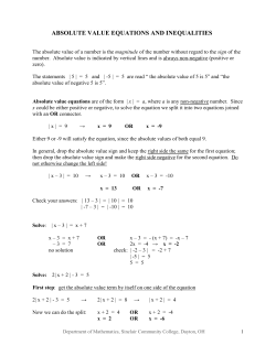
ABSOLUTE VALUE EQUATIONS AND INEQUALITIES
Factoring a polynomial over the integers, in one variable:
Adding and Subtracting Fractions
4.3 Absolute Value Equations y 10 x
Absolute Value Equations and Inequalities
Factoring and Solving Polynomial Equations What
© Copyright 2026
About abcdocz
DMCA / GDPR
Report