ABC
docz
Explore
Log in
Create new account
Download
Report
No category
Open Research Online The JCMT Gould Belt Survey: evidence for
3 Years exhibiting @ MWC
WAGGENER EDSTROM`S BRAND AGILITY INDEX AT
PDF - Mellinger Mennonite Church
Sunpartner Unveils its Latest Innovations
MUSEUM OF WESTERN COLORADO TRIPS & TOURS PO BOX
Erb Mennonite Church Welcome to
PDF - Mellinger Mennonite Church
Medical writing certification Exam Debuts This Year
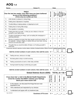
AOQ - English - My Doctor Online
AN APPROACH FOR OVERLAPPING CELL SEGMENTATION IN
© Copyright 2026
About abcdocz
DMCA / GDPR
Report