1. No category

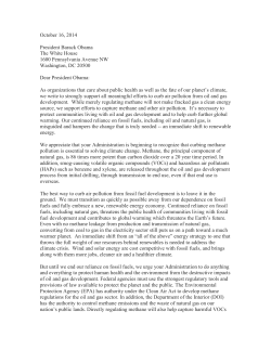
Open Research Online
The Open University’s repository of research publications
and other research outputs
Analysing the consistency of martian methane observations by investigation of global methane transport
Journal Article
How to cite:
Holmes, James A.; Lewis, Stephen R. and Patel, Manish R. (2015). Analysing the consistency of martian methane observations by investigation of global methane transport. Icarus, 257 pp. 23–32.
For guidance on citations see FAQs.
c 2015 The Authors
Version: Version of Record
Link(s) to article on publisher’s website:
http://dx.doi.org/doi:10.1016/j.icarus.2015.04.027
Copyright and Moral Rights for the articles on this site are retained by the individual authors and/or other copyright owners. For more information on Open Research Online’s data policy on reuse of materials please consult
the policies page.
oro.open.ac.uk
Icarus 257 (2015) 23–32
Contents lists available at ScienceDirect
Icarus
journal homepage: www.elsevier.com/locate/icarus
Analysing the consistency of martian methane observations
by investigation of global methane transport
James A. Holmes a,⇑, Stephen R. Lewis a, Manish R. Patel a,b
a
b
Department of Physical Sciences, The Open University, Milton Keynes MK7 6AA, UK
Space Science and Technology Department, STFC Rutherford Appleton Laboratory, Chilton, Didcot, Oxfordshire OX11 0QX, UK
a r t i c l e
i n f o
Article history:
Received 29 September 2014
Revised 15 April 2015
Accepted 15 April 2015
Available online 20 April 2015
Keywords:
Mars, atmosphere
Atmospheres, evolution
Meteorology
a b s t r a c t
Reports of methane on Mars at different times imply varying spatial distributions. This study examines
whether different observations are mutually consistent by using a global circulation model to investigate
the time evolution of methane in the atmosphere. Starting from an observed plume of methane, consistent with that reported in 2003 from ground-based telescopes, multiple simulations are analysed to
investigate what is required for consistency with an inferred methane signal from the Thermal
Emission Spectrometer made 60 sols later.
The best agreement between the existing observations is found using continued release from a solitary
source over Nili Fossae. While the peaks in methane over the Tharsis Montes, Elysium Mons and Nili
Fossae regions are well aligned with the retrievals, an extra peak on the south flank of the Isidis basin
is apparent in the model due to the prevailing eastward transport of methane. The absence of this feature
could indicate the presence of a fast-acting localised sink of methane.
These results show that the spatial and temporal variability of methane on Mars implied by observations could be explained by advection from localised time-dependent sources alongside a currently
unknown methane sink. Evidence is presented that a fast trapping mechanism for methane is required.
Trapping by a zeolite structure in dust particles is a suggested candidate warranting further investigation; this could provide a fast acting sink as required by this reconstruction.
Ó 2015 The Authors. Published by Elsevier Inc. This is an open access article under the CC BY license (http://
creativecommons.org/licenses/by/4.0/).
1. Introduction
Observations of methane on Mars have come from both
ground-based telescopes (Krasnopolsky et al., 2004; Mumma
et al., 2009) and orbiters (Formisano et al., 2004; Fonti and
Marzo, 2010) with maximum values ranging from 10 to 60 ppb.
More recently, the NASA Curiosity rover has measured a sudden
increase in methane in Gale crater to 7 ppb (Webster et al., 2015)
after previously providing an in situ local upper limit of 1.3 ppb
(Webster et al., 2013). The possibility of methane as a biomarker
for extraterrestrial life means its existence is significant, although
geological origin cannot be ruled out either (Atreya et al., 2007).
The reported observations from multiple instruments vary in
methane abundance and spatial distribution, with no general
agreement. Suggested processes to create methane in the
atmosphere range from volcanic hotspots and serpentinization to
cometary impacts and microorganisms with some of these sources
more feasible than others (Atreya et al., 2007). The origin of
source(s) of methane will not be addressed in this investigation.
⇑ Corresponding author.
E-mail address: [email protected] (J.A. Holmes).
The long lifetime of methane (300 years) implies it should
become well mixed in the atmosphere (Lefèvre and Forget,
2009). Additional destruction mechanisms are required to explain
the apparent variability observed. With a much shorter lifetime in
the atmosphere of 200 days, Lefèvre and Forget (2009) demonstrate the local enhancements of methane observed could be
potentially reconstructed. Destruction mechanisms theorised
include electrochemical processes during dust storms (Farrell
et al., 2006), a reactive surface due to a strong oxidiser such as
H2O2 (Atreya et al., 2006) and loss to the regolith (Gough et al.,
2010). Lefèvre and Forget (2009) dismiss electrochemical processes
due to the extreme bulk electric field needed and their effect on
other chemical species which are well simulated without these
added processes. Strong oxidation by H2O2 was investigated by
Gough et al. (2011) with the conclusion that a very deep soil layer
greater than 500 m in depth is required for rapid loss of methane
from the atmosphere. Loss to the regolith was also determined to
be too slow by Meslin et al. (2011). Surface loss of methane is reliant on the composition and structure of the martian regolith and
the uptake coefficient of the surface.
Mischna et al. (2011) investigated the creation of the plume
identified by Mumma et al. (2009), concluding that their best fit
http://dx.doi.org/10.1016/j.icarus.2015.04.027
0019-1035/Ó 2015 The Authors. Published by Elsevier Inc.
This is an open access article under the CC BY license (http://creativecommons.org/licenses/by/4.0/).
24
J.A. Holmes et al. / Icarus 257 (2015) 23–32
source indicated the plume of methane would have needed to form
in 1–2 sols. In their study, the potential of computer models in constraining the source of tracer plumes is clearly evident. Exploring
the consistency of past observations of methane measured by different instruments and at different points in time using source/sink
experiments is yet to be undertaken.
In this study a global circulation model (GCM) is used to investigate the consistency of past methane measurements by analysing
the transport of methane from source emission. The next section
describes the initial setup of the GCM. The simulations for the
investigation are detailed followed by results on the tracer transport diagnostics from the simulations. A comparison of the simulations and possible destruction mechanisms are then discussed. The
significance of this study regarding the NASA Curiosity rover
results is then described.
2. Method
This investigation uses the UK version of the LMD GCM which
has been developed in a collaboration of the Laboratoire de
Météorologie Dynamique, the Open University, the University of
Oxford and the Instituto de Astrofisica de Andalucia. This model
uses physical parameterisations (Forget et al., 1999) shared with
the LMD GCM. These are coupled to a spectral dynamical core
and semi-lagrangian advection scheme (Newman et al., 2002) to
transport tracers.
The dust distribution has been prescribed horizontally using an
interpolation of numerous sets of observations from orbiters and
landers using a kriging method (Montabone et al., 2015) and vertically using the Conrath dust profile. The model was truncated at
wavenumber 31 resulting in a 5° longitude–latitude grid with 32
vertical levels extending to an altitude of 100 km.
Methane is transported using a semi-lagrangian advection
scheme with mass conservation (Priestley, 1993). The advection
scheme uses wind fields updated by the dynamical core to determine the methane concentration at each model grid point every
30 min. For the best possible representation of atmospheric state,
temperature retrievals from the Thermal Emission Spectrometer
(TES) are assimilated (Lewis et al., 2007). The model ensures the
wind field is consistent with thermal data. This provides the best
constraint available on the transport of methane in the atmosphere
since there are no direct wind observations. Lewis et al. (2007) also
showed that actual transient wave behaviour seen in observations
is captured by the model when assimilating TES temperature profiles, rather than simply modifying the thermal state of the model
to produce transient modes of different strengths and locations.
For all simulations in this paper the initial column-average
methane mixing ratio is as shown in Fig. 1 in an effort to closely
match the observations in 2003 (LS = 122–155° Mars year [MY]
26) by Mumma et al. (2009). The observations cover only half
the surface. A simulation which included zero methane across all
latitudes from 180°E to 0° resulted in the same spatial distribution
as a simulation initialised as shown in Fig. 1 with slightly lower
levels in methane abundance. This suggests minimal sensitivity
of the simulation to the initial distribution of column-average
methane mixing ratio in this unobserved region.
Since column-averaged mixing ratios have been retrieved with
no information on the vertical structure, the initial mass mixing
ratio of methane was spread in the vertical using the weighting
function
(
f ðrÞ ¼
1
2
þ 12 cos
0;
10p ln ðrÞ
zmax
; if z 6 zmax
otherwise
where r ¼ p=ps is the sigma level of the model (atmospheric pressure p scaled by the surface pressure ps ) and zmax is the maximum
altitude for methane to still be present initially in the atmospheric
column. For the simulations, the maximum initial altitude of
methane was set at 10 km. Tests using 30 km and 50 km for zmax
showed little difference, in agreement with Mischna et al. (2011).
No initial assumption about whether the observations were
retrieved at the start, middle or end of the methane release is made.
Continued emission from the localised sources identified by
Mumma et al. (2009) is entirely plausible.
3. Simulations
To investigate the transport of methane by different surface
sources, four simulations are run as displayed in Table 1. The control run includes no additional sources or sinks of methane. The
MuS run includes a source identified by Mumma et al. (2009) over
Nili Fossae. The MiS run includes the best fit source emission from
Mischna et al. (2011) which is much more extensive in latitude
than the other simulations. The TS run is similar to the MuS run
but includes an additional source over the Tharsis region, where
initially methane was unobserved by Mumma et al. (2009).
The rate of emission in Table 1 has been calculated to closely
match the maximum methane abundance inferred by Fonti and
Marzo (2010) at LS = 180° MY 26 (hereafter FM10 signal). No additional constraint on where the maximum methane abundance is
located spatially on the globe for each simulation is made. Source
emission of any strength for the whole period in between the
observations resulted in the source still evident in the distribution
at LS = 180°. Therefore, a continued source emission must have
stopped within 50 sols of the original plume to allow time for
dispersion of methane over the source location. For ease of
analysis, the source emission occurs for the first 30 sol period
(LS = 148–164°) of each simulation (except the control run which
has no source). Where methane is being emitted by a surface
source, the methane mass mixing ratio q in the lowest level in
the atmosphere is given an additional increase after each timestep
of q ¼ q þ ðUm g DtÞ=Dp where Um is the source surface flux
(kg m2 s1), Dt is the timestep (s) and Dp is the pressure difference between the lowest two levels of the atmosphere (Pa). This
extra emission adds to the local methane mass and, along with
the methane already present in the atmosphere, is advected by
the transport scheme each timestep.
To match the maximum methane abundance in the FM10 signal, the MuS simulation required a single source strength of
Um ¼ 109 kg m2 s1 over the 5° 5° grid box, resulting in 85 kg
of methane added to the atmosphere every second. The formation
of the observed initial plume by Mumma et al. (2009) was investigated by Mischna et al. (2011) with their best fit conclusion being a
rapid build up of the plume over 1–2 sols before the observations.
To create the initial plume mass of 1.86 107 kg over 2 sols would
require over 100 kg of methane to be added to the atmosphere
each second. Also, a recent investigation by Stevens et al. (2015)
regarding the transport of methane in the martian subsurface indicate gas released by the destabilisation of methane clathrate
hydrates close to the surface could potentially provide a flux of
as much as 103 kg m2 s1 over a duration of less than half an MY.
4. Atmospheric transport of methane: A case study
This section describes the advection of methane in the four different simulations identified above in Table 1. The simulations
were all initialised with the exact same methane distribution
(Fig. 1) and all simulations, with the exception of the control run,
include a surface source of methane for the first 30 sols
(LS = 148–164° MY 26). In the following 30 sols (LS = 164–181°
MY 26), methane is simply advected in each simulation by
J.A. Holmes et al. / Icarus 257 (2015) 23–32
25
Fig. 1. Column-average methane mixing ratio at the start of the GCM simulation. The simulations begin at LS = 148° since the identified peaks in volume-average methane
mixing ratio were measured by Mumma et al. (2009) towards the end of their observation period in 2003 (LS = 122–155°).
Table 1
Details of the different simulations run over the 60 sol period investigated.
Simulation
Emission from LS = 148–164°?
Control
MuS
MiS
None
Surface emission at 2.5°N, 50°E
Surface emission in a parallelogram
covering 30–70°E and 37.5°S–37.5°N
Surface emission at 2.5°N, 50°E and
2.5°N, 90°W
TS
Rate of emission
[Um ] (kg m2 s1)
–
109
3.0 1011
0.5 109
transport processes with no further source emission. Since the
presence of methane does not affect the heating of the atmosphere,
the wind field is the same for all four simulations.
The zonal and meridional transport of methane is decomposed
into three separate constituents following Peixoto and Oort (1992)
as
½qa ¼ ½q½a þ ½q a þ ½q0 a0 ;
for a ¼ u; v
where u and v are the zonal and meridional wind respectively, the
overbar represents a time-average and the square brackets represent a zonal-average. Through this decomposition, the magnitude
of transport due to the mean circulation (½q½a), stationary eddies
(½q a ) and transient eddies (½q0 a0 ) can be compared. Deviations of
the variable from the time and zonal mean are represented by the
prime and star symbol respectively. Hinson (2006) found transient
eddies to at most have a period of 10 sols on Mars, therefore a 30 sol
time average is sufficient to sample multiple eddies. Results on the
transport of methane in this case study are split into the two previously mentioned 30 sol periods to distinguish between the time
period in which source emission occurs and after emission has
ceased.
4.1. LS = 148–164°: Source release
The vertically integrated zonal and meridional flux on each latitude circle for the control run are displayed in Fig. 2a and b respectively. Over this time period, the southern jet is beginning to
weaken after peak southern winter conditions and the northern
jet is beginning to form as autumnal equinox approaches.
The primary transport of methane zonally is eastward for all
simulations and is dominated by the mean circulation component.
The mean circulation of meridional flux (Fig. 2b) transports
mid-latitude methane towards the equator due to two roughly
symmetrical Hadley cells which both have a rising branch centred
near to the equator at this time of year. Transport by stationary and
transient eddies generally opposes the mean circulation resulting
in little overall transport of methane meridionally. Changes in
the zonal and meridional flux of methane from the control run
are attributed to changes in the local mass mixing ratio of methane
since the wind field is the same for all simulations.
With the source in the MuS run emitting for the 30 sol period,
the overall zonal transport is increased in both hemispheres. The
zonal transport just above the equator has increased considerably
to form an almost symmetrical pattern around the equator
(Fig. 2c). The large increase in mass of methane at the source location, coupled with weak surface winds, provides the peak in zonal
transport at 2.5°N. A stationary eddy south of Nili Fossae (Fig. 3a),
coupled to the mean circulation directly below the source location
(Fig. 3c), decrease the net eastward transport of methane just south
of the equator. This activity immediately below the source location
causes the elevated levels of methane to expand along a SW–NE
line centred on the source location. Fig. 3c also indicates that
methane is primarily transported eastward away from the source
in the mid-latitude regions of the north and south hemisphere over
Nili Fossae and Hellas basin respectively.
Two peaks in transport north and south of the equator are also
noticeable in the meridional flux (Fig. 2d). This feature is due to
transient eddies, which account for 65% of the meridional transport close to the equator. The identified peaks are almost entirely
due to the surface source emission, as evident in Fig. 3d, with the
meridional transport an order of magnitude larger than in the
control run (Fig. 2b). The continuous release of methane over time
provides peak transport directly north and south of the source by
weak surface meridional winds coupled to the increased mass of
methane.
The broad source in the MiS run acts primarily to enhance the
control run zonal flux profile, with an increase in zonal methane flux
26
J.A. Holmes et al. / Icarus 257 (2015) 23–32
Fig. 2. Vertically integrated zonal (left) and meridional (right) flux of methane for each latitude band in the control (a and b), MuS (c and d), MiS (e and f) and TS (g and h) runs
from LS = 148–164° MY 26. Note the change of scale for zonal and meridional flux in (a) and (b). Eastward and northward flux are positive.
of around 3 for most latitude bands peaking at 540 kg s1 (Fig. 2e).
The meridional flux of the MiS run in (Fig. 2f) displays large poleward
flow in the southern mid-latitudes due to a stationary eddy over
Hellas basin (Fig. 3b). This transport process is not as strong in the
MuS run since less methane is transported into poleward southern
latitudes by the MuS source. The zonal and meridional flux of
methane for the TS run have a similar pattern to the MuS run and
are displayed in Fig. 2g and h respectively. The TS simulation has a
source of half the strength of the MuS run alongside an additional
source over the Tharsis region with the same rate of emission (see
Table 1). A stationary eddy near the additional source over the
Tharsis region (Fig. 3b) increases the poleward flux of methane in
the northern hemisphere and is of similar strength to the transient
eddy transport (Fig. 2h). This stationary eddy also helps to provide
the increased zonal flux peak of 100 kg s1 at 30°N in Fig. 2g, when
compared to the MuS run (Fig. 2c). The methane emitted from the
source over the Tharsis region is transported north by the stationary
eddy and then eastward over Tempe Terra.
4.2. LS = 164–181°: Pure advection
The atmospheric conditions for this time period are similar to
the previous 30 sol period, but the peak zonal wind in each hemisphere are now at parity as the subsolar point drifts closer to the
equator. The northern atmospheric jet has an increased zonal peak
from 50 m s1 in the previous 30 sol period to 90 m s1 to now
match the strength of the southern jet.
Since there is no emission from methane sources in any of the
simulations, the zonal flux for all simulations is dominated by
the mean zonal circulation. The main differences in Fig. 4g occur
in where the peak zonal flux occur in latitude. For the MuS and
TS runs, the peak zonal flux is now in northern mid-latitudes since
a larger mass of methane exists in the northern hemisphere. As
also noted in the previous 30 sols, the zonal and meridional flux
of methane for the MuS and TS runs are very similar. The decreased
mass of methane in the control run, since no methane is added to
the atmosphere in the previous 30 sols, results in zonal flux peaks 5
J.A. Holmes et al. / Icarus 257 (2015) 23–32
27
Fig. 3. Longitude–latitude plots of time-average (a) zonal and (b) meridional wind deviation from the zonal mean (for all simulations), (c) the mean zonal circulation and (d)
meridional eddy transport of the MuS simulation for the time period LS = 148–164° MY 26. Black contour lines indicate topography. The source location for the MuS and TS
simulations are represented by black stars and by a shaded parallelogram for the MiS simulation in (a) and (b). The wind deviation is calculated from the surface up to 20 km
since the majority of methane is located here.
times weaker in strength when compared to the other three simulations. Since the MiS run included source emission in the last 30
sol period in the southern hemisphere (as well as in the northern
hemisphere), the peak zonal flux of methane is still in the southern
mid-latitudes, with Fig. 4 mirror-image of Fig. 4c and g in latitude.
A stationary wave is evident at 30°N with wavenumber 2,
caused by the topographical profile at this latitude (Fig. 5a). This
stationary wave accounts for 10% of the zonal transport at this
latitude. A combination of the mean circulation in the MuS run
(Fig. 5a) and the stationary wave in the 30°N latitude band creates
a build up of methane over three locations: north of the Tharsis
region, northwest of Nili Fossae and over Elysium Mons. This particular activity is evident in the TS run also and to a lesser extent in
the MiS run, with the increased zonal flux over Hellas basin stronger than the three regions of increased activity noted above due to
higher levels of methane in the southern hemisphere when compared to the MuS and TS runs.
Meridional transport of methane by stationary and transient
eddies in the MuS run is still marginally more effective than the
mean circulation at lower latitudes in the southern hemisphere
and throughout the northern hemisphere. Peak meridional transport is around half as strong as in the previous 30 sols for all simulations. Peak poleward transport has shifted to higher latitudes of
both hemispheres away from the equator. The MuS run has peak
poleward transport by stationary eddies just south of the equator.
This is due to increased southward transport by stationary eddies
located over Nili Fossae, the Tharsis region and south of Elysium
Mons (Fig. 5b). The increased mass of methane in the southern
hemisphere in the MiS run provides an overall equatorward meridional flux at 45°S. This is predominantly due to transport by the
mean meridional circulation (65%) with increased transport
equatorward on the north flank of the Argyre and Hellas basin in
the MiS run (Fig. 5d). This transport process in weaker in the
MuS and TS run due to lower levels of methane in these local
regions.
5. Discussion
In this section, the spatial distribution of methane from the simulations is studied to identify which simulation provides transport
of methane most consistent with an inferred signal by Fonti and
Marzo (2010). Surface adsorption (Meslin et al., 2011) added to
the best fit simulation is then explored followed by speculation
on a new method of methane removal from the atmosphere.
Evidence for the potential role of atmospheric dust in the temporary removal of methane is then discussed along with the relevance of this study regarding the latest measurements from the
NASA Curiosity rover.
5.1. Comparing simulated methane column to the inferred signal
The column-average methane mixing ratio at LS = 180° for the
MuS, MiS and TS run are displayed in Fig. 6a–c respectively. At this
time, a comparison to the FM10 signal (Fig. 6d) can be made. The
FM10 signal is restricted to between ±60° latitude gridded into
10° latitude by 10° longitude cells and show 3 distinct peaks: over
Arabia Terra, Elysium Mons and the Tharsis Montes region. For
ease of comparison, the model grid is interpolated on to the same
10° latitude by 10° longitude grid as the FM10 signal.
Running the control simulation until LS = 180° (not shown) provides a predominantly uniformly mixed atmosphere consistent
with previous studies (Lefèvre and Forget, 2009). The difference
between the maximum and minimum column-average methane
mixing ratio is around 5 ppb. The inclusion of a surface source in
the MuS run provides a vast improvement in the reconstruction
(Fig. 6a). The evolved distribution has a maximum methane column located over Tharsis Montes consistent with the FM10 signal
with no added constraint other than the strength of the source. The
general spatial distribution in the MuS simulation has a strong correlation with the FM10 signal (r(369) = 0.49, p < 0.01). The peaks in
28
J.A. Holmes et al. / Icarus 257 (2015) 23–32
Fig. 4. Vertically integrated zonal (left) and meridional (right) flux of methane for each latitude band in the control (a and b), MuS (c and d), MiS (e and f) and TS (g and h) runs
from LS = 164–181° MY 26. Note the change of scale for zonal and meridional flux in (a) and (b). Eastward and northward flux are positive.
column-average methane mixing ratio over the Tharsis Montes,
Arabia Terra and Elysium Mons regions are in line with the FM10
signal with a very strong correlation (r(52) = 0.77, p < 0.01). There
is an extra peak south of the Isidis basin which is difficult to reconcile due to the predominantly zonal advection of methane. To
remove this peak would require a strong localised sink of methane
acting frequently over this location, otherwise methane transported by westerly winds would quickly replenish the local
methane abundance. These results suggest the peaks in the FM10
signal need not have come from three localised source regions, as
suggested by Fonti and Marzo (2010), and could in fact have emanated from the single emission 60 sols earlier suggested by
Mumma et al. (2009).
The MiS run, displayed in Fig. 6b is less consistent with the
FM10 signal. The peak over the Tharsis Montes region is well
matched, but the peaks over Arabia Terra and Elysium Mons are
too far south. The broad source creates a higher abundance of
methane in the poleward southern latitudes, whereas the FM10
signal hint at decreasing values. The source suggested by
Mischna et al. (2011) was however an instantaneous ‘pulse’ and
therefore no further continuation of this broad release is suggested.
As the MuS source is located within the best fit creation of the
plume identified by Mischna et al. (2011), they are consistent only
if further emission (after the plume has initially been created) is
concentrated over the location of the MuS source.
The value of Um could potentially be reduced if there had been
increased initial methane levels over the Tharsis Montes region
(which were unobserved). This hypothesis has been tested by the
TS run, with similar success to the MuS run. The TS run however
has a more uniform level of methane across the peaks (Fig. 6c),
with the maximum methane abundance over Tharsis at a similar
level to the peaks over Arabia Terra and Elysium Mons. Sligthly elevated levels over Nili Fossae in the TS run, when compared to the
MuS run, indicate the methane emitted by the surface source over
the Tharsis region has predominantly been transported zonally as
far eastward as Nili Fossae over the 60 sol time period. With
J.A. Holmes et al. / Icarus 257 (2015) 23–32
29
Fig. 5. Longitude–latitude plots of time-average (a) zonal and (b) meridional wind deviation from the zonal mean (for all simulations), (c) mean zonal circulation for the MuS
simulation and (d) mean meridional circulation for the MiS simulation for the time period LS = 164–181° MY 26. Black contour lines indicate topography. The wind deviation
is calculated from the surface up to 20 km since the majority of methane is located here.
Fig. 6. Interpolated longitude–latitude plots of the column-average methane mixing ratio for the (a) MuS, (b) Mis and (c) TS simulation at LS = 180°. The corresponding
inferred methane signal from Fonti and Marzo (2010) is displayed in (d). Black contour lines indicate topography and the hatching in (d) indicates no data is available for this
location.
methane levels higher over the Tharsis region in the FM10 signal,
this is suggestive of a solitary source over Nili Fossae being sufficient for the reconstruction.
5.2. Inclusion of surface adsorption
Since there are still regions in the reconstruction which necessitate a destruction mechanism to reduce the local methane level
(west of Isidis basin for instance) a further simulation is run which
includes a proposed sink of methane. In this model (hereafter
MuSA), the same setup as the MuS run is used but adsorption of
methane on to the martian regolith with an adsorption rate consistent with previous investigations (Gough et al., 2010; Meslin et al.,
2011) is also introduced. Methane surficial removal is parame Þ=4 where ka is the
terised in the MuSA model by ka ¼ ðcqb Sv
adsorption rate (s1), c the uptake coefficient, qb the soil bulk den the mean
sity (kg m3), S the specific surface area (m2 kg1) and v
thermal speed of CH4 molecules (m s1) which is dependent on
temperature. Values for the soil bulk density and specific surface
area are 1300 kg m3 and 105 m2 kg1 respectively. This
30
J.A. Holmes et al. / Icarus 257 (2015) 23–32
mechanism is allowed to only affect the lowest layer of the atmosphere, and therefore simulate a surface sink of methane. It is an
irreversible adsorption and therefore less comprehensive than
the regolith diffusion model of Meslin et al. (2011). However, this
is considered to be sufficient for this study where emphasis is on
the net loss of methane from the atmosphere.
The uptake coefficient has been derived from laboratory
experiments on the JSC-1 Mars martian soil analogue (Gough
et al., 2010) and is temperature dependent, following
c ¼ expðð45:41 þ jDHobs jÞ=RTÞ where DHobs is a lower limit of
the enthalpy of adsorption (kJ mol1), T is the temperature and R
is the ideal gas constant (8.314 J K1 mol1). DHobs was experimentally determined by Gough et al. (2010) to have a value of
18.08 kJ mol1. The temperature dependence of the adsorption
rate results in increased adsorption at lower temperatures, with
a drop in the adsorption rate of two orders of magnitude from
150 to 280 K (Fig. 7a).
The adsorption occurs most strongly around the south pole,
extending up to 45°S latitude, where surface temperatures are at
their lowest at around 140–145 K (LS = 155–180° corresponds to
the end of southern winter). In the poleward northern latitudes,
adsorption only begins to have a noticeable effect after 30 sols.
Surficial adsorption of methane also occurs in the mid-latitudes
at high altitudes (such as around Olympus Mons) and due to the
diurnal variability of surface temperatures which can reach as
low as 150 K at Solis Planitia at nighttime.
The methane column at LS = 180° of the MuSA model is shown
in Fig. 7b and can be compared to the FM10 signal (Fig. 6d). The
pockets of lower methane abundance north of both the Argrye
and Hellas basins in the FM10 signal are difficult to reconcile even
using the MuSA model, suggesting even more localised
destruction.
The failure to reach the minimum levels, particularly considering there is no desorption in this model, implies the adsorption is
too slow as indicated by Meslin et al. (2011). The correlation
between the MuSA simulation and the FM10 signal decreases
(r(369) = 0.47, p < 0.01) when compared to the MuS simulation.
Trainer et al. (2010) concluded that trapping of methane in the
polar ice caps is practically negligible which also limits this
method of adsorption, since it occurs primarily over the polar
regions. The mechanism of surface adsorption for the destruction
of methane is evidently not a viable option.
et al., 2013). Spectral evidence from the dusty martian surface
(Ruff, 2004) along with CRISM measurements west of Nili Fossae
(Ehlmann et al., 2009) point to the possibility of zeolites being a
component of the martian surface and potentially the atmosphere.
Meslin et al. (2011) note that the adsorption rate for zeolites is larger than the standard martian regolith and the proposed mechanism here would be capable of removing methane from higher
altitudes than just the surface dust. Airborne dust also has an
advantage in potentially creating the spatial variations seen in
observations since a dust particle at higher altitude would be capable of quickly carrying the adsorbed methane away from the site
of adsorption.
Dust devils, which have been observed numerous times
(Thomas and Gierasch, 1985; Edgett and Malin, 2000; Greeley
et al., 2006), could also provide local-scale variations of methane,
and potentially induce at least partially the temporal and spatial
methane variations seen in the observations. The JSC-1 Mars analog contains no signature of zeolites and so any additional uptake
due to the presence of this substance is not present in the measured coefficient. Regarding the additional peak in the modelled
distribution on the south flank of the Isidis basin (see Fig. 6a),
flushing dust storms have been shown to start at the Isidis planitia
in model simulations (Mulholland et al., 2013). Although these primarily occur at LS = 210°, which is a short time after the FM10 signal, trapping of methane in these flushing dust storms could be
seen as a possible mechanism that could provide the fast removal
of methane in this localised region.
Full understanding of the spatial variability of zeolites is also
currently lacking. The zeolite proposed here would have to be a
specific designer material which preferentially adsorbs methane
over other atmospheric constituents such as CO2. Kim et al.
(2013) find only a couple of hypothetical zeolite structures which
could perform this task, and so the temporary removal mechanism
described here is currently not conclusive. Information on the rates
of trapping/release of methane by this proposed storage mechanism are currently unknown and would require further study.
Frequent observations of the methane distribution, with greater
certainty, would provide a more stringent comparison to
determine if this destruction mechanism is a viable option.
Future orbiter missions such as the ExoMars Trace Gas Orbiter
(TGO), scheduled for launch in 2016, will provide global methane
retrievals with good temporal and spatial coverage.
5.3. Methane removal by zeolite in martian dust?
5.4. Recent observations by the Curiosity rover
A potential methane sink which has been overlooked so far is
the possible presence of zeolite in atmospheric dust particles.
Methane reacts weakly with most surfaces, but some zeolites have
recently been suggested as a material that can trap methane (Kim
Potential evidence for atmospheric dust playing a role in the
removal of methane is seen in the latest measurements by the
NASA Curiosity rover (Webster et al., 2015). They have indicated
a possible anti-correlation between methane and atmospheric
Fig. 7. (a) Surface temperature plotted against the methane adsorption rate for the MuSA simulation. The formula for methane adsorption is the same as in (Meslin et al.,
2011). (b) Interpolated longitude–latitude plot of the column-average methane mixing ratio for the MuSA simulation at LS = 180°. Black contour lines indicate topography.
J.A. Holmes et al. / Icarus 257 (2015) 23–32
31
Fig. 8. Average visible dust optical depth (left) from the simulations for the 30 sol period leading up to the FM10 signal (right). Mars year is in reverse order from MY 26 (top
row) to MY 24 (bottom row).
opacity, suggestive that atmospheric dust could possibly be
involved in the process of removing methane from the atmosphere.
To test this hypothesis with the FM10 signal, the 30 sol average
dust optical depth leading up to LS = 180° is compared to the
FM10 signal for three Mars years (Fig. 8). There is a strong
anti-correlation coefficient of r(369) = 0.51 (p < 0.01) for MY 26
and r(428) = 0.40 (p < 0.01) for MY 24, with no correlation
evident for MY 25. The area north of Argyre basin, which is still
outstanding in all simulations, shows increased dust levels compared to the ambient atmospheric dust opacity. An atmospheric
sink related to the dust opacity would therefore lower the levels
over this region, more in line with the FM10 signal.
Lower levels of dust are present in the poleward northern and
mid latitudes, meaning these regions would be relatively unaffected if a currently unknown sink involving atmospheric dust is
present. The FM10 signal for multiple Mars years indicate the lowest levels of methane in the atmosphere occur around LS = 270°,
just after peak dust activity (Fonti and Marzo, 2010). Caution must
be taken with this analysis however due to the relatively large
FM10 signal uncertainty of ±25% for MY 24/26 and ±40% for
MY 25.
Following an initial upper limit of 1.3 ppb in Gale crater measured by the NASA Curiosity rover at around LS = 180° in MY 31
(Webster et al., 2013), more recent measurements have observed
a sudden increase to around 7 ppb (Webster et al., 2015) for a short
60 sol period. A case is made by Webster et al. (2015) that these
measurements best fit a local source which terminates quickly.
The latest measurements could potentially be consistent with
source emission and previous higher methane retrievals under certain conditions. Firstly, the plume observed by Mumma et al.
(2009) must not be an annual event, which is entirely plausible.
Secondly, the release of additional methane into the atmosphere
by surface emission or by other means must be fairly limited leading up to the Curiosity rover measurement by Webster et al.
(2015). A GCM can be used to investigate whether surface source
emission could account for the observed increase in this local
region, how strong it would need to be and where it is likely to
be spatially located.
Whether the conditions described above are credible is difficult
to know due to the lack of regular published global methane observations from the end of MY 26 to the present time. If a methane
sink is apparent on Mars, the lower levels of the Curiosity rover
measurements when compared to previous results (Mumma
et al., 2009; Fonti and Marzo, 2010) can be explained by a relative
lack of, or indeed complete absence of, methane source emission in
the intervening period. The ExoMars TGO will provide regular
methane observations in the future. The distribution of any spatial
variations seen by the ExoMars TGO can be studied by a GCM, in a
similar manner to this investigation, with the aim of identifying
how the spatial variations are formed.
6. Conclusions
During this investigation a GCM model is used as a tool to determine whether different observations of methane can be mutually
consistent. Although the passive model showed little similarity to
the observations, a simulation including additional source emission is shown to improve the match between previous observations. A potential source over the Tharsis region is plausible but
less consistent with both sets of observations than a solitary source
over Nili Fossae. An additional peak on the south flank of the Isidis
basin is not observed in the FM10 signal, but hard to remove from
the model due to the dominant zonal transport.
Including a surficial adsorption parameterisation alone did not
improve the reconstruction. A combination of both continued
source emission and adsorption however cannot be ruled out. A
zeolite structure present in dust storms is suggested here as a
new potential mechanism to trap methane, potentially bringing
the modelled behaviour of emitted methane into line with observations. Availability of adsorption sites on the dust particles would
provide an effective mechanism to destroy methane throughout
most of the lower atmosphere.
32
J.A. Holmes et al. / Icarus 257 (2015) 23–32
The strength of methane release and uptake is an issue which
remains unresolved. The synthesis of observations is improved
when the source over Nili Fossae continues to emit after the observations have been made, but for less than the whole 60 sol period
leading up to the FM10 signal. The efficiency of atmospheric mixing means constraints on the timescale and cessation of emissions
are key to accurately identifying the strength of methane release.
By investigating the transport diagnostics of methane, it is proposed that the three localised sources identified by Fonti and
Marzo (2010) for northern autumn MY 26 could in fact be a result
of the evolution of the methane plume observed earlier in the year
by Mumma et al. (2009). It is difficult to verify decisively the simulation results without regular observations in the time window,
especially regarding the latest measurement by the Curiosity rover.
A GCM can be used to investigate whether surface source emission
could account for the observed increase in Gale crater. The
ExoMars TGO, due for launch in 2016, will provide an ideal dataset
to analyse the validity of past observations and, in conjunction
with a GCM, explore the global distribution of martian methane.
Acknowledgments
The authors thank two anonymous referees for their constructive comments which have resulted in a substantial improvement
to the paper. JAH and SRL thank the UK Space Agency for support
under Grant ST/I003096/1, SRL thanks STFC for support under
Grant ST/J001597/1 and MRP thanks the UK Space Agency for support under Grant ST/I003061/1. Thanks also to Sergio Fonti and
Giuseppe Marzo for access to the TES methane retrievals. We are
grateful for an ongoing collaboration with François Forget and
coworkers at LMD and Franck Lefèvre at LATMOS. Model results
are available from the authors upon request. This work is funded
under the UKSA Aurora programme.
References
Atreya, S.K. et al., 2006. Oxidant enhancement in martian dust devils and storms:
Implications for life and habitability. Astrobiology 6, 439–450.
Atreya, S.K., Mahaffy, P.R., Wong, A.-S., 2007. Methane and related trace species on
Mars: Origin, loss, implications for life, and habitability. Planet. Space Sci. 55,
358–369.
Edgett, K.S., Malin, M.C., 2000. Martian dust raising and surface albedo controls:
Thin, dark (and sometimes bright) streaks and dust devils in MGS MOC high
resolution images. In: Lunar and Planetary Institute Science Conference
Abstracts, Lunar and Planetary Inst. Technical Report, vol. 31, p. 1073.
Ehlmann, B.L. et al., 2009. Identification of hydrated silicate minerals on Mars using
MRO-CRISM: Geologic context near Nili Fossae and implications for aqueous
alteration. J. Geophys. Res. (Planets) 114, E00D08.
Farrell, W.M., Delory, G.T., Atreya, S.K., 2006. Martian dust storms as a possible sink
of atmospheric methane. Geophys. Res. Lett. 33, L21203.
Fonti, S., Marzo, G.A., 2010. Mapping the methane on Mars. Astron. Astrophys. 512,
A51.
Forget, F. et al., 1999. Improved general circulation models of the martian
atmosphere from the surface to above 80 km. J. Geophys. Res. 104, 24155–
24176.
Formisano, V. et al., 2004. Detection of methane in the atmosphere of Mars. Science
306, 1758–1761.
Gough, R.V. et al., 2010. Methane adsorption on a martian soil analog: An abiogenic
explanation for methane variability in the martian atmosphere. Icarus 207,
165–174.
Gough, R.V. et al., 2011. Can rapid loss and high variability of martian methane be
explained by surface H2O2? Planet. Space Sci. 59, 238–246.
Greeley, R. et al., 2006. Active dust devils in Gusev crater, Mars: Observations from
the Mars Exploration Rover Spirit. J. Geophy. Res. (Planets) 111, E12S09.
Hinson, D.P., 2006. Radio occultation measurements of transient eddies in the
northern hemisphere of Mars. J. Geophys. Res. (Planets) 111, E05002.
Kim, J. et al., 2013. New materials for methane capture from dilute and mediumconcentration sources. Nature Comms. 4, 1694.
Krasnopolsky, V.A. et al., 2004. Detection of methane in the martian atmosphere:
Evidence for life? Icarus 172, 537–547.
Lefèvre, F., Forget, F., 2009. Observed variations of methane on Mars unexplained by
known atmospheric chemistry and physics. Nature 460, 720–723.
Lewis, S.R. et al., 2007. Assimilation of Thermal Emission Spectrometer atmospheric
data during the Mars Global Surveyor aerobraking period. Icarus 192, 327–347.
Meslin, P.-Y. et al., 2011. Little variability of methane on Mars induced by
adsorption in the regolith. Planet. Space Sci. 59, 247–258.
Mischna, M.A. et al., 2011. Atmospheric modeling of Mars methane surface releases.
Planet. Space Sci. 59, 227–237.
Montabone, L. et al., 2015. Eight-year climatology of dust optical depth on Mars.
Icarus 251, 65–95.
Mulholland, D.P., Read, P.L., Lewis, S.R., 2013. Simulating the interannual variability
of major dust storms on Mars using variable lifting thresholds. Icarus 223, 344–
358.
Mumma, M.J. et al., 2009. Strong release of methane on Mars in northern summer
2003. Science 323, 1041–1045.
Newman, C.E. et al., 2002. Modeling the martian dust cycle, 1. Representations of
dust transport processes. J. Geophys. Res. 107, 6-1–6-18.
Peixoto, J.P., Oort, A.H., 1992. Physics of Climate. American Institute of Physics.
Priestley, A., 1993. A quasi-conservative version of the semi-lagrangian advection
scheme. Mont. Weath. Rev. 121, 621–629.
Ruff, S.W., 2004. Spectral evidence for zeolite in the dust on Mars. Icarus 168, 131–
143.
Stevens, A.H., Patel, M.R., Lewis, S.R., 2015. Numerical modelling of the transport of
trace gases including methane in the subsurface of Mars. Icarus 250, 587–594.
Thomas, P., Gierasch, P., 1985. Dust devils on Mars. In: Lunar and Planetary Institute
Science Conference Abstracts, Lunar and Planetary Inst. Technical Report, vol.
16, p. 857.
Trainer, M.G. et al., 2010. Limits on the trapping of atmospheric CH4 in martian
polar ice analogs. Icarus 208, 192–197.
Webster, C.R. et al., 2013. Low upper limit to methane abundance on Mars. Science
342, 355–357.
Webster, C.R. et al., 2015. Mars methane detection and variability at Gale crater.
Science 347, 415–417.