
CHAPTER TWO Solutions for Section 2.1
2.1 SOLUTIONS
99
CHAPTER TWO
Solutions for Section 2.1
1. (a) The average rate of change is the slope of the secant line in Figure 2.1, which shows that this slope is positive.
(b) The instantaneous rate of change is the slope of the graph at x = 3, which we see from Figure 2.2 is negative.
f (x)
Slope = Average rate
of change of f
Slope = f ′ (3) = Rate
of change of f at 3
x
3
f (x)
x
7
3
Figure 2.1
Figure 2.2
2. (a) The function N = f (t) is decreasing when t = 1950. Therefore, f ′ (1950) is negative. That means that the number
of farms in the US was decreasing in 1950.
(b) The function N = f (t) is decreasing in 1960 as well as in 1980 but it is decreasing faster in 1960 than in 1980.
Therefore, f ′ (1960) is more negative than f ′ (1980).
3. (a) Let s = f (t).
(i) We wish to find the average velocity between t = 1 and t = 1.1. We have
Average velocity =
f (1.1) − f (1)
3.63 − 3
=
= 6.3 m/sec.
1.1 − 1
0.1
(ii) We have
Average velocity =
(iii) We have
f (1.01) − f (1)
3.0603 − 3
=
= 6.03 m/sec.
1.01 − 1
0.01
f (1.001) − f (1)
3.006003 − 3
=
= 6.003 m/sec.
1.001 − 1
0.001
(b) We see in part (a) that as we choose a smaller and smaller interval around t = 1 the average velocity appears to be
getting closer and closer to 6, so we estimate the instantaneous velocity at t = 1 to be 6 m/sec.
Average velocity =
4. For the interval 0 ≤ t ≤ 0.8, we have
Average velocity
0 ≤ t ≤ 0.8
Average velocity
0 ≤ t ≤ 0.2
Average velocity
0.2 ≤ t ≤ 0.4
!
=
s(0.8) − s(0)
6.5
=
= 8.125 ft/sec.
0.8 − 0
0.8
!
=
s(0.2) − s(0)
0.5
=
= 2.5 ft/sec.
0.2 − 0
0.2
!
=
s(0.4) − s(0.2)
1.3
=
= 6.5 ft/sec.
0.4 − 0.2
0.2
To find the velocity at t = 0.2, we find the average velocity to the right of t = 0.2 and to the left of t = 0.2 and
average them. So a reasonable estimate of the velocity at t = 0.2 is the average of 21 (6.5 + 2.5) = 4.5 ft/sec.
100
Chapter Two /SOLUTIONS
5. (a) The average velocity between t = 3 and t = 5 is
s(5) − s(3)
25 − 9
16
Distance
=
=
=
= 8 ft/sec.
Time
5−3
2
2
(b) Using an interval of size 0.1, we have
Instantaneous velocity
at t = 3
!
≈
≈
s(3.01) − s(3)
9.0601 − 9
=
= 6.01.
3.01 − 3
0.01
s(3.1) − s(3)
9.61 − 9
=
= 6.1.
3.1 − 3
0.1
Using an interval of size 0.01, we have
Instantaneous velocity
at t = 3
!
From this we guess that the instantaneous velocity at t = 3 is about 6 ft/sec.
6. (a) The average rate of change of a function over an interval is represented graphically as the slope of the secant line to
its graph over the interval. See Figure 2.3. Segment AB is the secant line to the graph in the interval from x = 0 to
x = 3 and segment BC is the secant line to the graph in the interval from x = 3 to x = 5.
We can easily see that slope of AB > slope of BC. Therefore, the average rate of change between x = 0 and
x = 3 is greater than the average rate of change between x = 3 and x = 5.
y
4
y
3
C
4
B
3
This slope is larger
?
2
2
1
1
A
x
1
2
3
4
x
5
1
2
Figure 2.3
3
4
5
Figure 2.4
(b) We can see from the graph in Figure 2.4 that the function is increasing faster at x = 1 than at x = 4. Therefore, the
instantaneous rate of change at x = 1 is greater than the instantaneous rate of change at x = 4.
(c) The units of rate of change are obtained by dividing units of cost by units of product: thousands of dollars/kilogram.
7. (a) The size of the tumor when t = 0 months is S(0) = 20 = 1 cubic millimeter. The size of the tumor when t = 6
months is S(6) = 26 = 64 cubic millimeters. The total change in the size of the tumor is S(6) − S(0) = 64 − 1 =
63 mm3 .
(b) The average rate of change in the size of the tumor during the first six months is:
Average rate of change =
S(6) − S(0)
64 − 1
63
=
=
= 10.5 cubic millimeters/month.
6−0
6
6
(c) We will consider intervals to the right of t = 6:
t (months)
6
6.001
6.01
6.1
S (cubic millimeters)
64
64.0444
64.4452
68.5935
2.1 SOLUTIONS
101
68.5935 − 64
4.5935
=
= 45.935
6.1 − 6
0.1
64.4452 − 64
0.4452
Average rate of change =
=
= 44.52
6.01 − 6
0.01
64.0444 − 64
0.0444
Average rate of change =
=
= 44.4
6.001 − 6
0.001
Average rate of change =
We can continue taking smaller intervals but the value of the average rate will not change much. Therefore, we can
say that a good estimate of the growing rate of the tumor at t = 6 months is 44.4 cubic millimeters/month.
8. (a) We have
6.45 − 4.08
= 0.079 billion people per year.
2005 − 1975
(b) To estimate f ′ (2005), we use the rate of change formula on an interval containing 2005:
Rate of change of population =
f ′ (2005) ≈
6.45 − 6.07
= 0.076 billion people per year.
2005 − 2000
9. We use the interval x = 2 to x = 2.01:
f ′ (2) ≈
f (2.01) − f (2)
52.01 − 52
25.4056 − 25
=
=
= 40.56
2.01 − 2
0.01
0.01
For greater accuracy, we can use the smaller interval x = 2 to x = 2.001:
f ′ (2) ≈
f (2.001) − f (2)
52.001 − 52
25.040268 − 25
=
=
= 40.268
2.001 − 2
0.001
0.001
10. (a) Figure 2.5 shows that for t = 2 the function g(t) = (0.8)t is decreasing. Therefore, g ′ (2) is negative.
g(t)
2
g(t) = (0.8)t
1
1
2
t
Figure 2.5
(b) To estimate g ′ (2) we take the small interval between t = 2 and t = 2.001 to the right of t = 2.
g ′ (2) ≈
g(2.001) − g(2)
0.82.001 − 0.82
0.6399 − 0.64
−0.0001
=
=
=
= −0.1
2.001 − 2
0.001
0.001
0.001
11. (a) f ′ (x) is negative when the function is decreasing and positive when the function is increasing. Therefore, f ′ (x) is
positive at C and G. f ′ (x) is negative at A and E. f ′ (x) is zero at B, D, and F .
(b) f ′ (x) is the largest when the graph of the function is increasing the fastest (i.e. the point with the steepest positive
slope). This occurs at point G. f ′ (x) is the most negative when the graph of the function is decreasing the fastest (i.e.
the point with the steepest negative slope). This occurs at point A.
12. We estimate f ′ (2) using the average rate of change formula on a small interval around 2. We use the interval x = 2 to
x = 2.001. (Any small interval around 2 gives a reasonable answer.) We have
f ′ (2) ≈
f (2.001) − f (2)
32.001 − 32
9.00989 − 9
=
=
= 9.89.
2.001 − 2
2.001 − 2
0.001
102
Chapter Two /SOLUTIONS
13. Since f ′ (x) = 0 where the graph is horizontal, f ′ (x) = 0 at x = d. The derivative is positive at points b and c, but the
graph is steeper at x = c. Thus f ′ (x) = 0.5 at x = b and f ′ (x) = 2 at x = c. Finally, the derivative is negative at points
a and e but the graph is steeper at x = e. Thus, f ′ (x) = −0.5 at x = a and f ′ (x) = −2 at x = e. See Table 2.1.
Thus, we have f ′ (d) = 0, f ′ (b) = 0.5, f ′ (c) = 2, f ′ (a) = −0.5, f ′ (e) = −2.
Table 2.1
x
f ′ (x)
d
0
b
0.5
c
2
a
−0.5
e
−2
14. (a) Since 75.2 percent live in the city in 1990 and 35.1 percent in 1890, we have
Average rate of change =
40.1
75.2 − 35.1
=
= 0.401.
1990 − 1890
100
Thus the average rate of change is 0.401 percent/year.
(b) By looking at the population in 1990 and 2000 we see that
Average rate of change =
79.0 − 75.2
3.8
=
= 0.38
2000 − 1990
10
which gives an average rate of change of 0.38 percent/year between 1990 and 2000. Alternatively, we look at the
population in 1980 and 1990 and see that
Average rate of change =
75.2 − 73.7
1.5
=
= 0.15
1990 − 1980
10
giving an average rate of change of 0.15 percent/year between 1980 and 1990. We see that the rate of change in the
year 1990 is somewhere between 0.38 and 0.15 percent/year. A good estimate is (0.38 + 0.15)/2 = 0.265 percent
per year. In fact, the definition of urban area was changed for the 2000 data, so this estimate should be used with care.
(c) By looking at the population in 1830 and 1860 we see that
Average rate of change =
10.8
19.8 − 9.0
=
= 0.36,
1860 − 1830
30
giving an average rate of change of 0.36 percent/year between 1830 and 1860. Alternatively we can look at the
population in 1800 and 1830 and see that
Average rate of change =
9.0 − 6.0
3.0
=
= 0.10.
1830 − 1800
30
giving an average rate of change of 0.10 percent/year between 1800 and 1830 . We see that the rate of change at the
year 1830 is somewhere between 0.10 and 0.36. This tells us that in the year 1830 the percent of the population in
urban areas is changing by a rate somewhere between 0.10 percent/year and 0.36 percent/year.
(d) Looking at the data we see that the percent gets larger as time goes by. Thus, the function appears to be always
increasing.
2.1 SOLUTIONS
103
15.
f (x) = x2
9
8
7
g(x) = x2 + 3
-
6
5
4
3
2
1
x
−4 −3 −2 −1
−1
1
2
3
4
Figure 2.6
(a) The tangent line to the graph of f (x) = x2 at x = 0 coincides with the x-axis and therefore is horizontal (slope
= 0). The tangent line to the graph of g(x) = x2 + 3 at x = 0 is the dashed line indicated in the figure and it also
has a slope equal to zero. Therefore both tangent lines at x = 0 are parallel.
We see in Figure 2.6 that the tangent lines at x = 1 appear parallel, and the tangent lines at x = 2 appear
parallel. The slopes of the tangent lines at any value x = a will be equal.
(b) Adding a constant shifts the graph vertically, but does not change the slope of the curve.
16. (a) Since the values of P go up as t goes from 4 to 6 to 8, we see that f ′ (6) appears to be positive. The percent of
households with cable television is increasing at t = 6.
(b) We estimate f ′ (2) using the difference quotient for the interval to the right of t = 2, as follows:
f ′ (2) ≈
63.4 − 61.5
1.9
∆P
=
=
= 0.95.
∆t
4−2
2
The fact that f ′ (2) = 0.95 tells us that the percent of households with cable television in the United States was
increasing at a rate of 0.95 percentage points per year when t = 2 (that means 1992).
Similarly:
∆P
68.9 − 67.8
1.1
f ′ (10) ≈
=
=
= 0.55.
∆t
12 − 10
2
The fact that f ′ (10) = 0.55 tells us that the percent of households in the United States with cable television was
increasing at a rate of 0.55 percentage points per year when t = 10 (that means 2000).
17. P ′ (0) is the derivative of the function P (t) = 200(1.05)t at t = 0. This is the same as the rate of change of P (t) at
t = 0. We estimate this by computing the average rate of change over intervals near t = 0.
If we use the intervals −0.001 ≤ t ≤ 0 and 0 ≤ t ≤ 0.001, we see that:
Average rate of change on − 0.001 ≤ t ≤ 0
=
Average rate of change on 0 ≤ t ≤ 0.001
=
200(1.05)0 − 200(1.05)−0.001
200 − 199.990
0.010
=
=
= 10,
0 − (−0.001)
0.001
0.001
200(1.05)0.001 − 200(1.05)0
200.010 − 200
0.010
=
=
= 10.
0.001 − 0
0.001
0.001
It appears that the rate of change of P (t) at t = 0 is 10, so we estimate P ′ (0) = 10.
18. The coordinates of A are (4, 25). See Figure 2.7. The coordinates of B and C are obtained using the slope of the tangent
line. Since f ′ (4) = 1.5, the slope is 1.5
104
Chapter Two /SOLUTIONS
Tangent line
B
1.5(0.2) = 0.3
0.2
A = (4, 25)
0.15
C
0.1
Figure 2.7
From A to B, ∆x = 0.2, so ∆y = 1.5(0.2) = 0.3. Thus, at C we have y = 25 + 0.3 = 25.3. The coordinates of
B are (4.2, 25.3).
From A to C, ∆x = −0.1, so ∆y = 1.5(−0.1) = −0.15. Thus, at C we have y = 25 − 0.15 = 24.85. The
coordinates of C are (3.9, 24.85).
19. (a) Since the point B = (2, 5) is on the graph of g, we have g(2) = 5.
(b) The slope of the tangent line touching the graph at x = 2 is given by
Slope =
Rise
5 − 5.02
−0.02
=
=
= −0.4.
Run
2 − 1.95
0.05
Thus, g ′ (2) = −0.4.
20. The answers to parts (a)–(d) are shown in Figure 2.8.
Slope= f ′ (3)
?
6
6
6
?
f (4) − f (2)
f (x)
Slope =
f (5)−f (2)
5−2
f (4)
?
1
2
3
4
x
5
Figure 2.8
21. (a) Since f is increasing, f (4) > f (3).
(b) From Figure 2.9, it appears that f (2) − f (1) > f (3) − f (2).
f (2) − f (1)
(c) The quantity
represents the slope of the secant line connecting the points on the graph at x = 1
2−1
and x = 2. This is greater than the slope of the secant line connecting the points at x = 1 and x = 3 which is
f (3) − f (1)
.
3−1
(d) The function is steeper at x = 1 than at x = 4 so f ′ (1) > f ′ (4).
2.1 SOLUTIONS
105
f (x)
f (3) − f (2)
6
?
6
f (2) − f (1)
66 ?
slope =
slope =
f (3)−f (1)
3−1
f (2)−f (1)
2−1
x
1
2
3
4
5
Figure 2.9
22. Using a difference quotient with h = 0.001, say, we find
1.001 ln(1.001) − 1 ln(1)
= 1.0005
1.001 − 1
2.001 ln(2.001) − 2 ln(2)
f ′ (2) ≈
= 1.6934
2.001 − 2
f ′ (1) ≈
The fact that f ′ is larger at x = 2 than at x = 1 suggests that f is concave up between x = 1 and x = 2.
23. The quantity f (0) represents the population on October 17, 2006, so f (0) = 300 million.
The quantity f ′ (0) represents the rate of change of the population (in millions per year). Since
1 person
1/106 million people
=
= 2.867 million people/year,
11 seconds
11/(60 · 60 · 24 · 365) years
so we have f ′ (0) = 2.867.
24. (a) f ′ (t) is negative or zero, because the average number of hours worked a week has been decreasing or constant over
time.
g ′ (t) is positive, because hourly wage has been increasing.
h′ (t) is positive, because average weekly earnings has been increasing.
(b) We use a difference quotient to the right for our estimates.
(i)
36.0 − 37.0
f ′ (1970) ≈
= −0.2 hours/year
1975 − 1970
34.3 − 34.3
f ′ (1995) ≈
= 0 hours/year.
2000 − 1995
In 1970, the average number of hours worked by a production worker in a week was decreasing at the rate of
0.2 hours per year. In 1995, the number of hours was not changing.
(ii)
4.73 − 3.40
= $0.27 per year
g ′ (1970) ≈
1975 − 1970
14.00 − 11.64
g ′ (1995) ≈
= $0.47 per year.
2000 − 1995
In 1970, the hourly wage was increasing at a rate of $0.27 per year. In 1995, the hourly wage was increasing at
a rate of $0.47 per year.
(iii)
170.28 − 125.80
= $8.90 per year
h′ (1970) ≈
1975 − 1970
480.41 − 399.53
h′ (1995) ≈
= $16.18 per year.
2000 − 1995
In 1970, average weekly earnings were increasing at a rate of $8.90 a year. In 1995, weekly earnings were
increasing at a rate of $16.18 a year.
106
Chapter Two /SOLUTIONS
Solutions for Section 2.2
1. Estimating the slope of the lines in Figure 2.10, we find that f ′ (−2) ≈ 1.0, f ′ (−1) ≈ 0.3, f ′ (0) ≈ −0.5, and f ′ (2) ≈
−1.
4
2
x
−4
0
−2
2
4
Figure 2.10
2. The graph is that of the line y = −2x + 2. The slope, and hence the derivative, is −2. See Figure 2.11.
4
x
4
−4
−4
Figure 2.11
3. See Figure 2.12.
4
x
4
−4
−4
Figure 2.12
4. See Figure 2.13.
4
4
−4
−4
Figure 2.13
x
2.2 SOLUTIONS
107
5. The slope of this curve is approximately −1 at x = −4 and at x = 4, approximately 0 at x = −2.5 and x = 1.5, and
approximately 1 at x = 0. See Figure 2.14.
4
x
4
−4
−4
Figure 2.14
6. See Figure 2.15.
4
4
−4
x
−4
Figure 2.15
7. See Figure 2.16.
4
4
−4
x
−4
Figure 2.16
f (x + h) − f (x)
. For this problem, we’ll take the average of the values obtained for h = 1
h
f (x + 1) − f (x − 1)
. Thus,
and h = −1; that’s the average of f (x + 1) − f (x) and f (x) − f (x − 1) which equals
2
f ′ (0) ≈ f (1) − f (0) = 13 − 18 = −5.
f ′ (1) ≈ (f (2) − f (0))/2 = (10 − 18)/2 = −4.
f ′ (2) ≈ (f (3) − f (1))/2 = (9 − 13)/2 = −2.
f ′ (3) ≈ (f (4) − f (2))/2 = (9 − 10)/2 = −0.5.
8. We know that f ′ (x) ≈
108
Chapter Two /SOLUTIONS
f ′ (4) ≈ (f (5) − f (3))/2 = (11 − 9)/2 = 1.
f ′ (5) ≈ (f (6) − f (4))/2 = (15 − 9)/2 = 3.
f ′ (6) ≈ (f (7) − f (5))/2 = (21 − 11)/2 = 5.
f ′ (7) ≈ (f (8) − f (6))/2 = (30 − 15)/2 = 7.5.
f ′ (8) ≈ f (8) − f (7) = 30 − 21 = 9.
The rate of change of f (x) is positive for 4 ≤ x ≤ 8, negative for 0 ≤ x ≤ 3. The rate of change is greatest at about
x = 8.
9. For x = 0, 5, 10, and 15, we use the interval to the right to estimate the derivative. For x = 20, we use the interval to the
left. For x = 0, we have
70 − 100
−30
f (5) − f (0)
=
=
= −6.
f ′ (0) ≈
5−0
5−0
5
Similarly, we find the other estimates in Table 2.2.
Table 2.2
x
f ′ (x)
10. (a) x3
(b) x4
(c) x5
0
5
10
15
20
−6
−3
−1.8
−1.2
−1.2
(d) x3
11. See Figure 2.17.
x
−1.5
f ′ (x)
Figure 2.17
12. This is a line with slope −2, so the derivative is the constant function f ′ (x) = −2. The graph is a horizontal line at
y = −2. See Figure 2.18.
1
x
1
2
−1
f ′ (x)
−2
Figure 2.18
13. See Figure 2.19.
f ′ (x)
x
2
4
Figure 2.19
2.2 SOLUTIONS
14. See Figure 2.20.
x
1
2
f ′ (x)
Figure 2.20
15. See Figure 2.21.
20
f ′ (x)
x
3
−3
−20
Figure 2.21
16. See Figure 2.22.
f ′ (x)
x
Figure 2.22
17. See Figure 2.23.
f ′ (x)
x
Figure 2.23
18. See Figure 2.24.
f ′ (x)
x
Figure 2.24
109
110
Chapter Two /SOLUTIONS
19. The graph is increasing for 0 < t < 10 and is decreasing for 10 < t < 20. One possible graph is shown in Figure 2.25.
The units on the horizontal axis are years and the units on the vertical axis are people.
people
f (t)
years
10
20
Figure 2.25
The derivative is positive for 0 < t < 10 and negative for 10 < t < 20. Two possible graphs are shown in
Figure 2.26. The units on the horizontal axes are years and the units on the vertical axes are people per year.
people/year
people/year
f ′ (t)
f ′ (t)
years
10
years
20
10
20
Figure 2.26
20. The value of g(x) is increasing at a decreasing rate for 2.7 < x < 4.2 and increasing at an increasing rate for x > 4.2.
7.4 − 6.0
∆y
=
= 2.8
∆x
5.2 − 4.7
9.0 − 7.4
∆y
=
= 3.2
∆x
5.7 − 5.2
between x = 4.7 and x = 5.2
between x = 5.2 and x = 5.7
Thus g ′ (x) should be close to 3 near x = 5.2.
21. The function is decreasing for x < −2 and x > 2, and increasing for −2 < x < 2. The matching derivative must be
negative (below the x-axis) for x < −2 and x > 2, positive (above the x-axis) for −2 < x < 2, and zero (on the x-axis)
for x = −2 and x = 2. The matching derivative is in graph VIII.
22. The function is a line with negative slope, so f ′ (x) is a negative constant, and the graph of f ′ (x) is a horizontal line below
the x-axis. The matching derivative is in graph IV.
23. The function is increasing for x < 2 and decreasing for x > 2. The corresponding derivative is positive (above the x-axis)
for x < 2, negative (below the x-axis) for x > 2, and zero at x = 2. The matching derivative is in graph II.
24. The function is increasing for x < −2 and decreasing for x > −2. The corresponding derivative is positive (above the
x-axis) for x < −2, negative (below the x-axis) for x > −2, and zero at x = −2. The derivatives in graphs VI and VII
both satisfy these requirements. To decide which is correct, consider what happens as x gets large. The graph of f (x)
approaches an asymptote, gets more and more horizontal, and the slope gets closer and closer to zero. The derivative in
graph VI meets this requirement and is the correct answer.
25. Since f ′ (x) > 0 for x < −1, f (x) is increasing on this interval.
Since f ′ (x) < 0 for x > −1, f (x) is decreasing on this interval.
Since f ′ (x) = 0 at x = −1, the tangent to f (x) is horizontal at x = −1.
One possible shape for y = f (x) is shown in Figure 2.27.
2.2 SOLUTIONS
111
x
−1
Figure 2.27
26. Since f ′ (x) > 0 for 1 < x < 3, we see that f (x) is increasing on this interval.
Since f ′ (x) < 0 for x < 1 and for x > 3, we see that f (x) is decreasing on these intervals.
Since f ′ (x) = 0 for x = 1 and x = 3, the tangent to f (x) will be horizontal at these x’s.
One of many possible shapes of y = f (x) is shown in Figure 2.28.
y
x
1
2
3
4
Figure 2.28
27. (a) Graph II
(b) Graph I
(c) Graph III
ln(1.1) − ln(1)
f (1.1) − f (1)
=
28. (a) f ′ (1) ≈
0.1
0.1
ln(2.1) − ln(2)
f (2.1) − f (2)
=
f ′ (2) ≈
0.1
0.1
f (3.1) − f (3)
ln(3.1) − ln(3)
f ′ (3) ≈
=
0.1
0.1
f (4.1) − f (4)
ln(4.1) − ln(4)
f ′ (4) ≈
=
0.1
0.1
ln(5.1) − ln(5)
f (5.1) − f (5)
=
f ′ (5) ≈
0.1
0.1
(b) It looks like the derivative of ln(x) is 1/x.
≈ 0.95.
≈ 0.49.
≈ 0.33.
≈ 0.25.
≈ 0.20.
29.
Table 2.3
x
f (x)
x
f (x)
x
f (x)
1.998
2.6587
2.998
8.9820
3.998
21.3013
1.999
2.6627
2.999
8.9910
3.999
21.3173
2.000
2.6667
3.000
9.0000
4.000
21.3333
2.001
2.6707
3.001
9.0090
4.001
21.3493
2.002
2.6747
3.002
9.0180
4.002
21.3653
Near 2, the values of f (x) seem to be increasing by 0.004 for each increase of 0.001 in x, so the derivative appears
0.004
= 4. Near 3, the values of f (x) are increasing by 0.009 for each step of 0.001, so the derivative appears to
to be 0.001
be 9. Near 4, f (x) increases by 0.016 for each step of 0.001, so the derivative appears to be 16. The pattern seems to be,
then, that at a point x, the derivative of f (x) = 31 x3 is f ′ (x) = x2 .
112
Chapter Two /SOLUTIONS
30.
y
(I)
y
(II)
3
3
1
1
x
1
−1−1
3
−3
3
1
3
y
(IV)
3
3
1
−1−1
1
−3
y
(III)
x
−1−1
1
x
1
3
−1−1
−3
x
−3
(a) III – f ′ (1) > 0 means that f is increasing near x = 1. f ′ decreasing means f is getting less steep, that is, f is
concave down.
(b) II – f ′ (1) > 0 means that f is increasing near x = 1. f ′ increasing means f is getting steeper, that is, f is concave
up.
(c) IV – f ′ (1) < 0 means that f is decreasing near x = 1. f ′ decreasing means f is sloping down more, that is, f is
concave down.
(d) I – f ′ (1) < 0 means that f is decreasing near x = 1. f ′ increasing means f is sloping down less, that is, f is concave
up.
31. (a) t = 3
(b) t = 9
(c) t = 14
(d)
V ′ (t)
1
15
3
6
9
12
18
t
−2
Solutions for Section 2.3
1. In Leibniz notation the derivative is dC/dW and the units are dollars per pound.
2. In Leibniz notation the derivative is dD/dt and the units are feet per minute.
3. In Leibniz notation the derivative is dP/dH and the units are dollars per hour.
4. In Leibniz notation the derivative is dN/dD and the units are gallons per mile.
5. (a) The 12 represents the weight of the chemical; therefore, its units are pounds. The 5 represents the cost of the chemical;
therefore, its units are dollars. The statement f (12) = 5 means that when the weight of the chemical is 12 pounds,
the cost is 5 dollars.
(b) We expect the derivative to be positive since we expect the cost of the chemical to increase when the weight bought
increases.
(c) Again, 12 is the weight of the chemical in pounds. The units of the 0.4 are dollars/pound since it is the rate of change
of the cost as a function of the weight of the chemical bought. The statement f ′ (12) = 0.4 means that the cost is
increasing at a rate of 0.4 dollars per pound when the weight is 12 pounds, or that an additional pound will cost about
an extra 40 cents.
6. (a) The statement f (5) = 18 means that when 5 milliliters of catalyst are present, the reaction will take 18 minutes.
Thus, the units for 5 are ml while the units for 18 are minutes.
(b) As in part (a), 5 is measured in ml. Since f ′ tells how fast T changes per unit a, we have f ′ measured in minutes/ml.
If the amount of catalyst increases by 1 ml (from 5 to 6 ml), the reaction time decreases by about 3 minutes.
2.3 SOLUTIONS
113
7. (a) If the price is $150, then 2000 items will be sold.
(b) If the price goes up from $150 by $1 per item, about 25 fewer items will be sold. Equivalently, if the price is decreased
from $150 by $1 per item, about 25 more items will be sold.
8. The derivative f ′ (10) is the slope of the tangent line to the curve at t = 10. See Figure 2.29. Taking two points on the
tangent line, we calculate its slope:
100 − 70
Slope ≈
= 6.
5
′
Since the slope is about 6, we have f (10) ≈ 6 cm/yr. At t = 10, the sturgeon was growing in length at a rate of about 6
centimeters a year.
length (cm)
150
100 − 70 = 30
100
6
?
50
5
10
5-
15
20
t (years)
Figure 2.29
9. (Note that we are considering the average temperature of the yam, since its temperature is different at different points
inside it.)
(a) It is positive, because the temperature of the yam increases the longer it sits in the oven.
(b) The units of f ′ (20) are ◦ F/min. The statement f ′ (20) = 2 means that at time t = 20 minutes, the temperature T
would increase by approximately 2◦ F if the yam is in the oven an additional minute.
10. Let p be the rating points earned by the CBS Evening News, let R be the revenue earned in millions of dollars, and let
R = f (p). When p = 4.3,
Rate of change of revenue ≈
$5.5 million
= 55 million dollars/point.
0.1 point
Thus
f ′ (4.3) ≈ 55.
11. (a) The units of compliance are units of volume per units of pressure, or liters per centimeter of water.
(b) The increase in volume for a 5 cm reduction in pressure is largest between 10 and 15 cm. Thus, the compliance
appears maximum between 10 and 15 cm of pressure reduction. The derivative is given by the slope, so
Compliance ≈
0.70 − 0.49
= 0.042 liters per centimeter.
15 − 10
(c) When the lung is nearly full, it cannot expand much more to accommodate more air.
12. (a) The units of lapse rate are the same as for the derivative dT /dz, namely (units of T )/(units of z) = ◦ C/km.
(b) Since the lapse rate is 6.5, the derivative of T with respect to z is dT /dz = −6.5◦ C/km. The air temperature drops
about 6.5◦ for every kilometer you go up.
13. (a) This means that investing the $1000 at 5% would yield $1649 after 10 years.
(b) Writing g ′ (r) as dB/dr, we see that the units of dB/dr are dollars per percent (interest). We can interpret dB as
the extra money earned if interest rate is increased by dr percent. Therefore g ′ (5) = dB
|
≈ 165 means that
dr r=5
the balance, at 5% interest, would increase by about $165 if the interest rate were increased by 1%. In other words,
g(6) ≈ g(5) + 165 = 1649 + 165 = 1814.
14. The units of f ′ (x) are feet/mile. The derivative, f ′ (x), represents the rate of change of elevation with distance from the
source, so if the river is flowing downhill everywhere, the elevation is always decreasing and f ′ (x) is always negative. (In
fact, there may be some stretches where the elevation is more or less constant, so f ′ (x) = 0.)
114
Chapter Two /SOLUTIONS
15. (a) Since W = f (c) where W is weight in pounds and c is the number of Calories consumed per day:
f (1800) = 155
means that
consuming 1800 Calories per day
results in a weight of 155 pounds.
f ′ (2000) = 0
means that
consuming 2000 Calories per day causes
neither weight gain nor loss.
(b) The units of dW/dc are pounds/(Calories/day).
16. (a) The statement f (200) = 1300 means that it costs $1300 to produce 200 gallons of the chemical.
(b) The statement f ′ (200) = 6 means that when the number of gallons produced is 200, costs are increasing at a rate of
$6 per gallon. In other words, it costs about $6 to produce the next (the 201st ) gallon of the chemical.
17. (a)
(b)
(c)
(d)
(e)
Positive, since weight increases as the child gets older.
f (8) = 45 tells us that when the child is 8 years old, the child weighs 45 pounds.
The units of f ′ (a) are lbs/year. f ′ (a) tells the rate of growth in lbs/years at age a.
f ′ (8) = 4 tells us that the 8-year-old child is growing at a rate of 4 lbs/year.
As a increases, f ′ (a) will decrease since the rate of growth slows down as the child grows up.
18. (a) An additional dollar per year of government purchases increases national output for the year by about $0.60. The
derivative is called a fiscal policy multiplier because if government purchases increase by x dollars per year, then
national output increases by about 0.60x dollars per year.
(b) An additional tax dollar collected per year decreases national output for the year by about $0.26. The derivative
is called a fiscal policy multiplier because if government tax revenues increase by x dollars per year, then national
output decreases by about 0.26x dollars per year.
19. Let f (t) be the age of onset of Alzheimer’s, in weeks, of a typical man who retires at age t years. The derivative f ′ (t) has
units weeks/year. The study reports that each additional year of employment is associated with about a six week later age
of onset, that is, f ′ (t) ≈ 6.
20. (a) Since f ′ (c) is negative, the function P = f (c) is decreasing: pelican eggshells are getting thinner as the concentration, c, of PCBs in the environment is increasing.
(b) The statement f (200) = 0.28 means that the thickness of pelican eggshells is 0.28 mm when the concentration of
PCBs in the environment is 200 parts per million (ppm).
The statement f ′ (200) = −0.0005 means that the thickness of pelican eggshells is decreasing (eggshells are becoming thinner) at a rate of 0.0005 mm per ppm of concentration of PCBs in the environment when the concentration
of PCBs in the environment is 200 ppm.
21. (a) kilograms per week
(b) At week 24 the fetus is growing at a rate of 0.096 kg/week, or 96 grams per week.
22. (a) The tangent line to the weight graph is steeper at 36 weeks then at 20 weeks, so g ′ (36) is greater than g ′ (20).
(b) The fetus increases its weight more rapidly at week 36 than at week 20.
23. Compare the secant line to the graph from week 0 to week 40 to the tangent lines at week 20 and week 36.
(a) At week 20 the secant line is steeper than the tangent line. The instantaneous weight growth rate is less than the
average.
(b) At week 36 the tangent line is steeper than the secant line. The instantaneous weight growth rate is greater than the
average.
24. We estimate the derivatives at 20 and 36 weeks by drawing tangent lines to the weight graph, shown in Figure 2.30, and
calculating their slopes.
(a) Two points on the tangent line at 20 weeks are (16, 0) and (40, 1.5). Thus,
g ′ (20) ≈
1.5 − 0
= 0.0625 kg/week.
40 − 16
(b) Two points on the tangent line at 36 weeks are (24, 0) and (40, 3.0). Thus,
g ′ (36) ≈
3−0
= 0.19 kg/week.
40 − 24
(c) The average rate of growth is the slope of the secant line from (0, 0) to (40, 3.1). Thus,
Average rate of change =
3.1 − 0
= 0.078kg/week.
40 − 0
2.3 SOLUTIONS
115
weight (kilograms)
3.5
3
2.5
2
Slope = g ′ (20)
1.5
1
0.5
0
Slope = g ′ (36)
age of fetus (weeks after last menstruation)
4
8 12 16 20 24 28 32 36 40
Figure 2.30
25. Since we do not have information beyond t = 25, we will assume that the function will continue to change at the same
rate. Therefore,
f (26) ≈ f (25) + f ′ (25)
= 3.6 + (−0.2) = 3.4.
Since 30 = 25 + 5, then
f (30) ≈ f (25) + f ′ (25)(5)
= 3.6 + (−0.2)(5) = 2.6.
26. Using the approximation ∆y ≈ f ′ (x)∆x with ∆x = 2, we have ∆y ≈ f ′ (20) · 2 = 6 · 2, so
f (22) ≈ f (20) + f ′ (20) · 2 = 345 + 6 · 2 = 357.
27. (a) The statement f (8) = 5.1 means that annual net sales for the Hershey Company were 5.1 billion dollars in 2008.
The statement f ′ (8) = 0.22 tells us that in 2008, annual net sales were increasing at a rate of 0.22 billion dollars per
year, or 220 million dollars per year.
(b) Since sales were 5.1 billion in 2008 and increasing at 0.22 billion dollars per year, we estimate that, four years later
in 2012,
Sales in 2012 ≈ 5.1 + 4(0.22) = 5.98 billion dollars.
Thus f (12) = 5.98, so annual net sales for the Hershey Company are projected to be 5.98 billion dollars in 2012.
This prediction assumes that the growth rate remains constant.
28. (a) The statement f (5) = 249 tells us that M = 249 when t = 5, and the statement f ′ (5) = 6.5 tells us that the rate
of change of M is 6.5 when t = 5. In terms of meat production, this means that in 2005, world meat production was
249 million metric tons and increasing at a rate of 6.5 million metric tons per year.
(b) We assume that the growth rate remains constant until t = 10. Since production in 2005 is 249 million metric tons
and is increasing at 6.5 million metric tons a year, we expect production in 2010 to be approximately
f (10) ≈ 249 + 5 · 6.5 = 249 + 32.5 = 281.5 million metric tons.
29. (a) The statement f (140) = 120 means that a patient weighing 140 pounds should receive a dose of 120 mg of the
painkiller. The statement f ′ (140) = 3 tells us that if the weight of a patient increases by one pound (from 140
pounds), the dose should be increased by about 3 mg.
(b) Since the dose for a weight of 140 lbs is 120 mg and at this weight the dose goes up by about 3 mg for one pound, a 145
lb patient should get about an additional 3(5) = 15 mg. Thus, for a 145 lb patient, the correct dose is approximately
f (145) ≈ 120 + 3(5) = 135 mg.
30. (a) The statement f (20) = 0.36 means that 20 minutes after smoking a cigarette, there will be 0.36 mg of nicotine in
the body. The statement f ′ (20) = −0.002 means that 20 minutes after smoking a cigarette, nicotine is leaving the
body at a rate 0.002 mg per minute. The units are 20 minutes, 0.36 mg, and −0.002 mg/minute.
116
Chapter Two /SOLUTIONS
(b)
f (21) ≈ f (20) + change in f in one minute
= 0.36 + (−0.002)
= 0.358
f (30) ≈ f (20) + change in f in 10 minutes
= 0.36 + (−0.002)(10)
= 0.36 − 0.02
= 0.34
31. (a) Since t represents the number of days from now, we are told f (0) = 80 and f ′ (0) = 0.50.
(b)
f (10) ≈ value now + change in value in 10 days
= 80 + 0.50(10)
= 80 + 5
= 85.
In 10 days, we expect that the mutual fund will be worth about $85 a share.
32. (a) The tangent line is shown in Figure 2.31. Two points on the line are (0, 16) and (3.2, 0). Thus
Slope =
0 − 16
= −5 (cm/sec)/kg.
3.2 − 0
(b) Since 50 grams = 0.050 kg, the contraction velocity changes by about −5(cm/sec)/kg · 0.050kg = −0.25 cm/sec.
The velocity is reduced by about 0.25 cm/sec or 2.5 mm/sec.
(c) Since v(x) is the contraction velocity in cm/sec with a load of x kg, we have v ′ (2) = −5.
contraction velocity (cm/sec)
30
25
20
v(x)
15
10
5
x, load opposing
1
2
3
4
contraction (kg)
Figure 2.31
33. (a) The tangent line is shown in Figure 2.32. Two points on the line are (0, 0.75) and (2.5, 5). The
Slope =
5 − 0.75
= 1.7 (liters/minute)/hour.
2.5 − 0
(b) The rate of change of the pumping rate is the slope of the tangent line. One minute = 1/60 hour, so in one minute
the
(liter/minute)
1
Pumping rate increases by about 1.7
·
hour = 0.028 liter/minute.
hour
60
′
(c) Since g(t) is the pumping rate in liters/minute at time t hours, we have g (2) = 1.7.
2.3 SOLUTIONS
117
pumping rate of heart
(liters pumped per minute)
5
g(t)
4
3
2
1
0
1
2
3
t (hours)
Figure 2.32
34. Units of C ′ (r) are dollars/percent. Approximately, C ′ (r) means the additional amount needed to pay off the loan when
the interest rate is increased by 1%. The sign of C ′ (r) is positive, because increasing the interest rate will increase the
amount it costs to pay off a loan.
35. (a) The company hopes that increased advertising always brings in more customers instead of turning them away. Therefore, it hopes f ′ (a) is always positive.
(b) ¡¡¡¡¡¡¡ .mine If f ′ (100) = 2, it means that if the advertising budget is $100,000, each extra dollar spent on advertising
will bring in about $2 ======= If f ′ (100) = 2, it means that if the advertising budget is $100,000, each extra dollar
spent on advertising will bring in about $2 ¿¿¿¿¿¿¿ .r3088 worth of sales. If f ′ (100) = 0.5, each dollar above $100
thousand spent on advertising will bring in about $0.50 worth of sales.
(c) If f ′ (100) = 2, then as we saw in part (b), spending slightly more than $100,000 will increase revenue by an amount
greater than the additional expense, and thus more should be spent on advertising. If f ′ (100) = 0.5, then the increase
in revenue is less than the additional expense, hence too much is being spent on advertising. The optimum amount
to spend, a, is an amount that makes f ′ (a) = 1. At this point, the increases in advertising expenditures just pay for
themselves. If f ′ (a) < 1, too much is being spent; if f ′ (a) > 1, more should be spent.
36. (a) See part (b).
(b) See Figure 2.33.
concentration of enzymes
Normal level
-
f′ > 0
-
time
f′ < 0
Figure 2.33
(c) The derivative, f ′ , is the rate at which the concentration is increasing or decreasing. We see that f ′ is positive at the
start of the disease and negative toward the end. In practice, of course, f ′ cannot be measured directly. Checking the
value of C in blood samples taken on consecutive days allows us to estimate f ′ (t):
f ′ (t) ≈ f (t + 1) − f (t) =
f (t + 1) − f (t)
.
(t + 1) − t
37. The consumption rates (kg/week) are the rates at which the quantities are decreasing, that is, −1 times the derivatives of
the storage functions. To compare rates at a given time, compare the steepness of the tangent lines to the graphs at that
time.
(a) At 3 weeks, the tangent line to the fat storage graph is steeper than the tangent line to the protein storage graph.
During the third week, fat is consumed at a greater rate than protein.
(b) At 7 weeks, the protein storage graph is steeper than the fat storage graph. During the seventh week, protein is
consumed at a greater rate than fat.
118
Chapter Two /SOLUTIONS
38. Where the graph is linear, the derivative of the fat storage function is constant. The derivative gives the rate of fat consumption (kg/week). Thus, for the first four weeks the body burns fat at a constant rate.
39. The fat consumption rate (kg/week) is the rate at which the quantity of fat is decreasing, that is, −1 times the derivative
of the fat storage function. We estimate the derivatives at 3, 6, and 8 weeks by drawing tangent lines to the storage graph,
shown in Figure 2.34, and calculating their slopes.
(a) The tangent line at 3 weeks is the storage graph itself since that part of the graph is straight. Two points on the tangent
line are (0, 12) and (4, 4). Then
4 − 12
Slope =
= −2.0 kg/week.
4−0
The consumption rate is 2.0 kg/week.
(b) Two points on the tangent line are (0, 4.7) and (8, 0.1). Then,
Slope =
0.1 − 4.7
= −0.6 kg/week.
8−0
The consumption rate is 0.6 kg/week.
(c) Two points on the tangent line are (0, 2.7) and (8, 0.6). Then
Slope =
The consumption rate is 0.3 kg/week.
0.6 − 2.7
= −0.3 kg/week.
8−0
quantities of stored fat (kilograms)
12
10
8
6
4
2
0
1
2
3
4
5
6
7
8
weeks of starvation
Figure 2.34: Rates of consumption are −1 times slopes of tangent
lines
40. The body changes from burning more fat than protein to burning more protein. This is done by reducing the rate at which
it burns fat and simultaneously increasing the rate at which it burns protein. The physiological reason is that the body has
begun to run out of fat.
41. The graph of fat storage is linear for four weeks, then becomes concave up. Thus, the derivative of fat storage is constant
for four weeks, then increases. This matches graph I.
The graph of protein storage is concave up for three weeks, then becomes concave down. Thus, the derivative of
protein storage is increasing for three weeks and then becomes decreasing. This matches graph II.
42. (a) The statement f (9) = 740 tells us that there were 740 million acres of rain forest in Brazil in 2009. The derivative
f ′ (9) = −2.7 tells us that in 2009 Brazil’s rain forests were shrinking at a rate of 2.7 million acres per year.
(b) We have
−2.7
f ′ (9)
Relative rate of change =
=
= −0.00365.
f (9)
740
Brazil’s rain forests are shrinking at a rate of 0.365% per year.
43. Since t = 4 is the end of April 2009, we have f (4) = 200 million users. We use a difference quotient with t = 2 for the
end of February 2009 and t = 4 for the end of April 2009 to estimate the derivative:
f (4) − f (2)
200 − 175
=
= 12.5 million users per month.
4−2
4−2
To estimate the relative rate of change, we use
f ′ (4) ≈
Relative rate of change =
f ′ (4)
12.5
=
= 0.0625 per month.
f (4)
200
The number of active Facebook users at the end of April 2009 was 200 million. The number was increasing at 12.5
million users per month, which represents a relative growth rate of 6.25% per month.
2.4 SOLUTIONS
119
44. (a) At 2 1/2 months, the baby weighs 5.67 kilograms.
(b) At 2 1/2 months, the baby’s weight is increasing at a relative rate of 13% per month.
45. Estimating the relative rate of change using ∆t = 0.01, we have
1 f (4.01) − f (4)
1 4.012 − 42
1 ∆f
≈
= 2
= 0.50.
f ∆t
f (4)
0.01
4
0.01
46. Let P = f (t).
(a) Estimating the relative rate of change using ∆t = 1, we have
1 f (4) − f (3)
1 ∆P
=
= 0.0356197 = 3.56% per year
P ∆t
f (3)
1
(b) With ∆t = 0.1 we have
1 ∆P
1 f (3.1) − f (3)
=
= 0.0350613 = 3.51% per year
P ∆t
f (3)
0.1
(c) With ∆t = 0.01 we have
1 f (3.01) − f (3)
1 ∆P
=
= 0.0350061 = 3.50% per year
P ∆t
f (3)
0.01
In fact, the relative rate of change at t = 3 of the population for this city is exactly 0.035.
Solutions for Section 2.4
1. (a) Since the graph is below the x-axis at x = 2, the value of f (2) is negative.
(b) Since f (x) is decreasing at x = 2, the value of f ′ (2) is negative.
(c) Since f (x) is concave up at x = 2, the value of f ′′ (2) is positive.
2. At B both dy/dx and d2 y/dx2 could be positive because y is increasing and the graph is concave up there. At all the
other points one or both of the derivatives could not be positive.
3. f ′ (x) > 0
f ′′ (x) > 0
4. f ′ (x) = 0
f ′′ (x) = 0
5. f ′ (x) < 0
f ′′ (x) = 0
6. f ′ (x) < 0
f ′′ (x) > 0
7. f ′ (x) > 0
f ′′ (x) < 0
8. f ′ (x) < 0
f ′′ (x) < 0
9.
(a)
(b)
f (x)
x
f (x)
x
120
Chapter Two /SOLUTIONS
(d)
(c)
f (x)
f (x)
x
x
10. The derivative of w(t) appears to be negative since the function is decreasing over the interval given. The second derivative, however, appears to be positive since the function is concave up, i.e., it is decreasing at a decreasing rate.
11. The derivative, s′ (t), appears to be positive since s(t) is increasing over the interval given. The second derivative also
appears to be positive or zero since the function is concave up or possibly linear between t = 1 and t = 3, i.e., it is
increasing at a non-decreasing rate.
12. The graph must be everywhere decreasing and concave up on some intervals and concave down on other intervals. One
possibility is shown in Figure 2.35.
x
Figure 2.35
13. Since all advertising campaigns are assumed to produce an increase in sales, a graph of sales against time would be
expected to have a positive slope.
A positive second derivative means the rate at which sales are increasing is increasing. If a positive second derivative
is observed during a new campaign, it is reasonable to conclude that this increase in the rate sales are increasing is caused
by the new campaign–which is therefore judged a success. A negative second derivative means a decrease in the rate at
which sales are increasing, and therefore suggests the new campaign is a failure.
14. (a) The function appears to be decreasing and concave down, and so we conjecture that f ′ is negative and that f ′′ is
negative.
(b) We use difference quotients to the right:
f ′ (2) ≈ 137−145
= −4
4−2
f ′ (8) ≈ 56−98
=
−21.
10−8
15. (a) The derivative, f ′ (t), appears to be positive since the number of cars is increasing. The second derivative, f ′′ (t),
appears to be positive during the period 1940–1980 because the rate of change is increasing. For example, between
1940 and 1950, the rate of change is (40.3 − 27.5)/10 = 1.28 million cars per year, while between 1950 and 1960,
the rate of change is 2.14 million cars per year.
(b) We use the average rate of change formula on the interval 1970 to 1980 to estimate f ′ (1975):
f ′ (1975) ≈
121.6 − 89.2
32.4
=
= 3.24.
1980 − 1970
10
We estimate that f ′ (1975) ≈ 3.24 million cars per year. The number of passenger cars in the US was increasing at a
rate of about 3.24 million cars per year in 1975.
16. The derivative is positive on those intervals where the function is increasing and negative on those intervals where the
function is decreasing. Therefore, the derivative is positive on the intervals 0 < t < 0.4 and 1.7 < t < 3.4, and negative
on the intervals 0.4 < t < 1.7 and 3.4 < t < 4.
The second derivative is positive on those intervals where the graph of the function is concave up and negative on
those intervals where the graph of the function is concave down. Therefore, the second derivative is positive on the interval
1 < t < 2.6 and negative on the intervals 0 < t < 1 and 2.6 < t < 4.
2.4 SOLUTIONS
121
17. The derivative is positive on those intervals where the function is increasing and negative on those intervals where the
function is decreasing. Therefore, the derivative is positive on the interval −2.3 < t < −0.5 and negative on the interval
−0.5 < t < 4.
The second derivative is positive on those intervals where the graph of the function is concave up and negative on
those intervals where the graph of the function is concave down. Therefore, the second derivative is positive on the interval
0.5 < t < 4 and negative on the interval −2.3 < t < 0.5.
18. This graph is increasing for all x, and is concave down to the left of 2 and concave up to the right of 2. One possible
answer is shown in Figure 2.36:
x
2
Figure 2.36
19. The two points at which f ′ = 0 are A and B. Since f ′ is nonzero at C and D and f ′′ is nonzero at all four points, we get
the completed Table 2.4:
Table 2.4
Point
f
f′
f ′′
A
−
0
+
B
+
0
−
C
+
−
−
D
−
+
+
20. (b). The positive first derivative tells us that the temperature is increasing; the negative second derivative tells us that the
rate of increase of the temperature is slowing.
21. (e). Since the smallest value of f ′ (t) was 2◦ C/hour, we know that f ′ (t) was always positive. Thus, the temperature rose
all day.
22. Since f (2) = 5, the graph goes through the point (2, 5). Since f ′ (2) = 1/2, the slope of the curve is 1/2 when it passes
through this point. Since f ′′ (2) > 0, the graph is concave up at this point. One possible graph is shown in Figure 2.37.
Many other answers are also possible.
5
x
2
Figure 2.37
122
Chapter Two /SOLUTIONS
23. To the right of x = 5, the function starts by increasing, since f ′ (5) = 2 > 0 (though f may subsequently decrease) and
is concave down, so its graph looks like the graph shown in Figure 2.38. Also, the tangent line to the curve at x = 5 has
slope 2 and lies above the curve for x > 5. If we follow the tangent line until x = 7, we reach a height of 24. Therefore,
f (7) must be smaller than 24, meaning 22 is the only possible value for f (7) from among the choices given.
y
T
24
f (x)
20
x
5
7
Figure 2.38
24. (a) The EPA will say that the rate of discharge is still rising. The industry will say that the rate of discharge is increasing
less quickly, and may soon level off or even start to fall.
(b) The EPA will say that the rate at which pollutants are being discharged is leveling off, but not to zero—so pollutants
will continue to be dumped in the lake. The industry will say that the rate of discharge has decreased significantly.
25. (a) Let N (t) be the number of people below the poverty line. See Figure 2.39.
N (t)
t
Figure 2.39
(b) dN/dt is positive, since people are still slipping below the poverty line. d2 N/dt2 is negative, since the rate at which
people are slipping below the poverty line, dN/dt, is decreasing.
26. (a) dP/dt > 0 and d2 P/dt2 > 0.
(b) dP/dt < 0 and d2 P/dt2 > 0 (but dP/dt is close to zero).
27. (a)
utility
quantity
(b) As a function of quantity, utility is increasing but at a decreasing rate; the graph is increasing but concave down. So
the derivative of utility is positive, but the second derivative of utility is negative.
28. (a) IV, (b) III, (c) II, (d) I, (e) IV, (f) II
2.5 SOLUTIONS
123
Solutions for Section 2.5
1. (a) Marginal cost is the derivative C ′ (q), so its units are dollars/barrel.
(b) It costs about $3 more to produce 101 barrels of olive oil than to produce 100 barrels.
2. The marginal cost is approximated by the difference quotient
MC ≈
4830 − 4800
∆C
=
= 3.
∆q
1305 − 1295
The marginal cost is approximately $3 per item.
3. Marginal cost = C ′ (q). Therefore, marginal cost at q is the slope of the graph of C(q) at q. We can see that the slope at
q = 5 is greater than the slope at q = 30. Therefore, marginal cost is greater at q = 5. At q = 20, the slope is small,
whereas at q = 40 the slope is larger. Therefore, marginal cost at q = 40 is greater than marginal cost at q = 20.
4. Drawing in the tangent line at the point (10000, C(10000)) we get Figure 2.40.
$
C(q)
20,000
10,000
q
0
10,000
Figure 2.40
We see that each vertical increase of 2500 in the tangent line gives a corresponding horizontal increase of roughly
6000. Thus the marginal cost at the production level of 10,000 units is
Slope of tangent line
C ′ (10,000) =
to C(q) at q = 10,000
=
2500
= 0.42.
6000
This tells us that after producing 10,000 units, it will cost roughly $0.42 to produce one more unit.
5. Drawing in the tangent line at the point (600, R(600)), we get Figure 2.41.
$
R(q)
20,000
10,000
q
0
600
Figure 2.41
We see that each vertical increase of 2500 in the tangent line gives a corresponding horizontal increase of roughly
150. The marginal revenue at the production level of 600 units is
R′ (600) =
Slope of tangent line
to R(q) at q = 600
=
2500
= 16.67.
150
This tells us that after producing 600 units, the revenue for producing the 601st product will be roughly $16.67.
124
Chapter Two /SOLUTIONS
6. (a) For q = 500
Profit = π(500) = R(500) − C(500) = 9400 − 7200 = 2200 dollars.
(b) As production increases from q = 500 to q = 501,
∆R ≈ R′ (500)∆q = 20 · 1 = 20 dollars,
∆C ≈ C ′ (500)∆q = 15 · 1 = 15 dollars,
Thus
Change in profit = ∆π = ∆R − ∆C = 20 − 15 = 5 dollars.
7. We have
C(2500) − C(2000)
3825 − 3640
=
= $0.37/ton.
2500 − 2000
500
This means that recycling the 2001st ton of paper will cost around $0.37. The marginal cost is smallest at the point where
the derivative of the function is smallest. Thus the marginal cost appears to be smallest on the interval 2500 ≤ q ≤ 3000.
C ′ (2000) ≈
8. The slope of the revenue curve is greater than the slope of the cost curve at both q1 and q2 , so the marginal revenue is
greater at both production levels.
9. (a) We can approximate C(16) by adding C ′ (15) to C(15), since C ′ (15) is an estimate of the cost of the 16th item.
C(16) ≈ C(15) + C ′ (15) = $2300 + $108 = $2408.
(b) We approximate C(14) by subtracting C ′ (15) from C(15), where C ′ (15) is an approximation of the cost of producing the 15th item.
C(14) ≈ C(15) − C ′ (15) = $2300 − $108 = $2192.
10. We know M C ≈ C(1,001) − C(1,000). Therefore, C(1,001) ≈ C(1,000) + M C or C(1,001) ≈ 5000 + 25 = 5025
dollars.
Since we do not know M C(999), we will assume that M C(999) = M C(1,000). Therefore:
M C(999) = C(1,000) − C(999).
Then:
C(999) ≈ C(1,000) − M C(999) = 5,000 − 25 = 4,975 dollars.
Alternatively, we can reason that
M C(1,000) ≈ C(1,000) − C(999),
so
Now for C(1,000), we have
Since 1,100 − 1,000 = 100,
C(999) ≈ C(1,000) − M C(1,000) = 4,975 dollars.
C(1,100) ≈ C(1,000) + M C · 100.
C(1,100) ≈ 5,000 + 25 × 100 = 5,000 + 2,500 = 7,500 dollars.
11. (a) The cost to produce 50 units is $4300 and the marginal cost to produce additional items is about $24 per unit.
Producing two more units (from 50 to 52) increases cost by $48. We have
C(52) ≈ 4300 + 24(2) = $4348.
(b) When q = 50, the marginal cost is $24 per item and the marginal revenue is $35 per item. The profit on the 51st item
is approximately 35 − 24 = $11.
(c) When q = 100, the marginal cost is $38 per item and the marginal revenue is $35 per item, so the company loses
about $3 by producing the 101st item. Since the company will lose money, it should not produce the 101st item.
12. At q = 50, the slope of the revenue is larger than the slope of the cost. Thus, at q = 50, marginal revenue is greater than
marginal cost and the 50th bus should be added. At q = 90 the slope of revenue is less than the slope of cost. Thus, at
q = 90 the marginal revenue is less than marginal cost and the 90th bus should not be added.
2.5 SOLUTIONS
125
13. (a) At q = 2000, we have
Profit = R(2000) − C(2000) = 7780 − 5930 = 1850 dollars.
(b) If q increases from 2000 to 2001,
∆R ≈ R′ (2000) · ∆q = 2.5 · 1 = 2.5 dollars,
∆C ≈ C ′ (2000) · ∆q = 2.1 · 1 = 2.1 dollars,
Thus,
Change in profit = ∆R − ∆C ≈ 2.5 − 2.1 = 0.4 dollars.
Since increasing production increases profit, the company should increase production.
(c) By a calculation similar to that in part (b), as q increases from 2000 to 2001,
Change in profit ≈ 4.32 − 4.77 = −0.45 dollars.
Since increasing production reduces the profit, the company should decrease production.
14. (a) At q = 2.1 million,
Profit = π(2.1) = R(2.1) − C(2.1) = 6.9 − 5.1 = 1.8 million dollars.
(b) If ∆q = 0.04,
Change in revenue, ∆R ≈ R′ (2.1)∆q = 0.7(0.04) = 0.028 million dollars = $28,000.
Thus, revenues increase by about $28,000.
(c) If ∆q = −0.05,
Change in revenue, ∆R ≈ R′ (2.1)∆q = 0.7(−0.05) = −0.035 million dollars = −$35,000.
Thus, revenues decrease by about $35,000.
(d) We find the change in cost by a similar calculation. For ∆q = 0.04,
Change in cost, ∆C ≈ C ′ (2.1)∆q = 0.6(0.04) = 0.024 million dollars = $24,000
Change in profit, ∆π ≈ $28,000 − $24,000 = $4000.
Thus, increasing production 0.04 million units increases profits by about $4000.
For ∆q = −0.05,
Change in cost, ∆C ≈ C ′ (2.1)∆q = 0.6(−0.05) = −0.03 million dollars = −$30,000
Change in profit, ∆π ≈ −$35,000 − (−$30,000) = −$5000.
Thus, decreasing production 0.05 million units decreases profits by about $5000.
15. (a) The value of C(0) represents the fixed costs before production, that is, the cost of producing zero units, incurred for
initial investments in equipment, and so on.
(b) The marginal cost decreases slowly, and then increases as quantity produced increases.
marginal
cost
q1
q2
q
(c) Concave down implies decreasing marginal cost, while concave up implies increasing marginal cost.
(d) An inflection point of the cost function is (locally) the point of maximum or minimum marginal cost.
(e) One would think that the more of an item you produce, the less it would cost to produce extra items. In economic
terms, one would expect the marginal cost of production to decrease, so we would expect the cost curve to be concave down. In practice, though, it eventually becomes more expensive to produce more items, because workers and
resources may become scarce as you increase production. Hence after a certain point, the marginal cost may rise
again. This happens in oil production, for example.
126
Chapter Two /SOLUTIONS
Solutions for Chapter 2 Review
1. (a) Let s = f (t).
(i) We wish to find the average velocity between t = 1 and t = 1.1. We have
Average velocity =
(ii) We have
f (1.1) − f (1)
7.84 − 7
=
= 8.4 m/sec.
1.1 − 1
0.1
7.0804 − 7
f (1.01) − f (1)
=
= 8.04 m/sec.
1.01 − 1
0.01
Average velocity =
(iii) We have
f (1.001) − f (1)
7.008004 − 7
=
= 8.004 m/sec.
1.001 − 1
0.001
(b) We see in part (a) that as we choose a smaller and smaller interval around t = 1 the average velocity appears to be
getting closer and closer to 8, so we estimate the instantaneous velocity at t = 1 to be 8 m/sec.
Average velocity =
2.
Slope
−3
−1
0
1/2
1
2
Point
F
C
E
A
B
D
3. (a) From Figure 2.42 we can see that for x = 1 the value of the function is decreasing. Therefore, the derivative of f (x)
at x = 1 is negative.
4
3
2
f (x) = 2 − x3
1
x
−4 −3 −2 −1
−1
1
2
3
4
−2
−3
Figure 2.42
(b) f ′ (1) is the derivative of the function at x = 1. This is the rate of change of f (x) = 2 − x3 at x = 1. We estimate
this by computing the average rate of change of f (x) over intervals near x = 1.
Using the intervals 0.999 ≤ x ≤ 1 and 1 ≤ x ≤ 1.001, we see that
Average rate of change
on 0.999 ≤ x ≤ 1
=
[2 − 13 ] − [2 − 0.9993 ]
1 − 1.002997
=
= −2.997,
1 − 0.999
0.001
0.996997 − 1
[2 − 1.0013 ] − [2 − 13 ]
=
= −3.003.
on 1 ≤ x ≤ 1.001
1.001 − 1
0.001
′
It appears that the rate of change of f (x) at x = 1 is approximately −3, so we estimate f (1) = −3.
Average rate of change =
4. Using the interval 1 ≤ x ≤ 1.001, we estimate
f (1.001) − f (1)
3.0033 − 3.0000
=
= 3.3
0.001
0.001
x
The graph of f (x) = 3 is concave up so we expect our estimate to be greater than f ′ (1).
f ′ (1) ≈
5. The slope is positive at A and D; negative at C and F . The slope is most positive at A; most negative at F .
6. (a) Since the point A = (7, 3) is on the graph of f , we have f (7) = 3.
(b) The slope of the tangent line touching the curve at x = 7 is given by
Slope =
Thus, f ′ (7) = 4.
3.8 − 3
0.8
Rise
=
=
= 4.
Run
7.2 − 7
0.2
SOLUTIONS to Review Problems For Chapter Two
127
7. (a) Let s = f (t).
(i) We wish to find the average velocity between t = 1 and t = 1.1. We have
Average velocity =
f (1.1) − f (1)
0.808496 − 0.909297
=
= −1.00801 m/sec.
1.1 − 1
0.1
Average velocity =
f (1.01) − f (1)
0.900793 − 0.909297
=
= −0.8504 m/sec.
1.01 − 1
0.01
(ii) We have
(iii) We have
f (1.001) − f (1)
0.908463 − 0.909297
=
= −0.834 m/sec.
1.001 − 1
0.001
(b) We see in part (a) that as we choose a smaller and smaller interval around t = 1 the average velocity appears to be
getting closer and closer to −0.83, so we estimate the instantaneous velocity at t = 1 to be −0.83 m/sec. In this case,
more estimates with smaller values of h would be very helpful in making a better estimate.
Average velocity =
8. See Figure 2.43.
f ′ (x)
x
Figure 2.43
9. This is a line with slope 1, so the derivative is the constant function f ′ (x) = 1. The graph is the horizontal line y = 1.
See Figure 2.44.
f ′ (x)
1
x
3
−3
Figure 2.44
10. See Figure 2.45.
f ′ (x)
4
Figure 2.45
x
128
Chapter Two /SOLUTIONS
11. See Figure 2.46.
1
−1
x
2
3
4
f ′ (x)
Figure 2.46
12. See Figure 2.47.
x
f ′ (x)
Figure 2.47
13. See Figure 2.48.
f ′ (x)
x
Figure 2.48
14. (a) We use the interval to the right of x = 2 to estimate the derivative. (Alternately, we could use the interval to the left
of 2, or we could use both and average the results.) We have
f ′ (2) ≈
f (4) − f (2)
24 − 18
6
=
= = 3.
4−2
4−2
2
We estimate f ′ (2) ≈ 3.
(b) We know that f ′ (x) is positive when f (x) is increasing and negative when f (x) is decreasing, so it appears that
f ′ (x) is positive for 0 < x < 4 and is negative for 4 < x < 12.
15. (a) The function f is increasing where f ′ is positive, so for x1 < x < x3 .
(b) The function f is decreasing where f ′ is negative, so for 0 < x < x1 or x3 < x < x5 .
16. kilograms/meter
17. The statement f (20) = 57 means that when t = 20, we have P = 57. This tells us that in 2002, 57% of households had
a personal computer. The statement f ′ (20) = 3 tells us that in 2002, the percent of households with a personal computer
is increasing at a rate of about 3% a year.
18. (a) The yam is cooling off so T is decreasing and f ′ (t) is negative.
(b) Since f (t) is measured in degrees Fahrenheit and t is measured in minutes, df /dt must be measured in units of
◦
F/min.
SOLUTIONS to Review Problems For Chapter Two
129
19. (a) The statement f (15) = 200 tells us that when the price is $15, we sell about 200 units of the product.
(b) The statement f ′ (15) = −25 tells us that if we increase the price by $1 (from 15), we will sell about 25 fewer units
of the product.
20. The derivative f ′ (6) is the slope of the tangent line at t = 6. See Figure 2.49. We estimate that the slope of the tangent
line is about (250 − 50)/8 = 25. We have f ′ (6) ≈ 25 megawatts per year. In 1996, the world solar energy output was
increasing at a rate of about 25 megawatts per year.
solar power (megawatts)
300
6
200
250 − 50 = 250
100
?
2
4
6
8
8
10
t (years since 1990)
-
Figure 2.49
21. Using ∆x = 1, we can say that
f (21) = f (20) + change in f (x)
≈ f (20) + f ′ (20)∆x
= 68 + (−3)(1)
= 65.
Similarly, using ∆x = −1,
f (19) = f (20) + change in f (x)
≈ f (20) + f ′ (20)∆x
= 68 + (−3)(−1)
= 71.
Using ∆x = 5, we can write
f (25) = f (20) + change in f (x)
≈ f (20) + (−3)(5)
= 68 − 15
= 53.
22. (a) The derivative f ′ (t) appears to be positive, because according to the table, gold production is increasing.
(b) The derivative (or rate of change) appears to be greatest between 1996 and 1999.
(c) We have
82.9 − 82.6
f ′ (2002) ≈
= 0.1 million ounces/year.
2002 − 1999
In 2002, gold production was increasing at a rate of approximately 0.1 million ounces per year.
(d) In 2002, gold production was 82.9 million ounces and was increasing at a rate of 0.1 million ounces each year.
Therefore, in 2003 (one year later), we have
f (2003) ≈ 82.9 + 0.1 = 83.0 million ounces,
and in 2010 (8 years later), we have
f (2010) ≈ 82.9 + 0.1(8) = 83.7 million ounces.
We estimate that gold production in 2003 is 83.0 million troy ounces and gold production in 2010 is 83.7 million
troy ounces.
130
Chapter Two /SOLUTIONS
23. Moving away slightly from the center of the hurricane from a point 15 kilometers from the center moves you to a point
with stronger winds. For example, the wind is stronger at 15.1 kilometers from the center of the hurricane than it is at 15
kilometers from the center.
24. After falling 20 meters the speed of the rock is increasing at a rate of 0.5 meters/second per meter.
25. Since f (t) = 1.291(1.006)t , we have
f (6) = 1.291(1.006)6 = 1.338.
′
To estimate f (6), we use a small interval around 6:
f ′ (6) ≈
1.291(1.006)6.001 − 1.291(1.006)6
f (6.001) − f (6)
=
= 0.008.
6.001 − 6
0.001
We see that f (6) = 1.338 billion people and f ′ (6) = 0.008 billion (that is, 8 million) people per year. Since t = 6 in
2009, this model predicts that the population of China will be about 1,338,000,000 people in 2009 and growing at a rate
of about 8,000,000 people per year at that time.
26. Since B is measured in dollars and t is measured in years, dB/dt is measured in dollars per year. We can interpret dB
as the extra money added to your balance in dt years. Therefore dB/dt represents how fast your balance is growing, in
units of dollars/year.
27. (a) If f ′ (t) > 0, the depth of the water is increasing. If f ′ (t) < 0, the depth of the water is decreasing.
(b) The depth of the water is increasing at 20 cm/min when t = 30 minutes.
(c) We use 1 meter = 100 cm, 1 hour = 60 min. At time t = 30 minutes
Rate of change of depth = 20
cm
cm 60 min
1m
= 20
·
·
= 12 meters/hour.
min
min
1 hr
100 cm
28. We have ∆h = h(6003) − h(6000) ≈ h′ (6000)∆x = (0.5)(3) = 1.5 meters. The elevation increases approximately
1.5 meters as the climber moves from a position 6000 meters from the start of the trail to a position 6003 meters from the
start. Thus the climber’s elevation increases from 8000 meters to about 8001.5 meters. The new elevation is about 8001.5
meters above sea level.
29. The fact that f (80) = 0.05 means that when the car is moving at 80 km/hr is it using 0.05 liter of gasoline for each
kilometer traveled.
The derivative f ′ (v) is the rate of change of gasoline consumption with respect to speed. That is, f ′ (v) tells us how
the consumption of gasoline changes as speeds vary. We are told that f ′ (80) = 0.0005. This means that a 1-kilometer
increase in speed results in an increase in consumption of about 0.0005 liter per km. At higher speeds, the vehicle burns
more gasoline per km traveled than at lower speeds.
30. (a) Since the traffic flow is the number of cars per hour, it is the slope of the graph of C(t). It is greatest where the graph
of the function C(t) is the steepest and increasing. This happens at approximately t = 3 hours, or 7am.
(b) By reading the values of C(t) from the graph we see:
Average rate of change
C(2) − C(1)
1000 − 400
600
=
=
=
= 600 cars/hour,
on 1 ≤ t ≤ 2
2−1
1
1
2000 − 1000
1000
C(3) − C(2)
Average rate of change
=
=
= 1000 cars/hour.
=
3−2
1
1
on 2 ≤ t ≤ 3
A good estimate of C ′ (2) is the average of the last two results. Therefore:
C ′ (2) ≈
(600 + 1000)
1600
=
= 800 cars/hour.
2
2
(c) Since t = 2 is 6 am, the fact that C ′ (2) ≈ 800 cars/hour means that the traffic flow at 6 am is about 800 cars/hour.
31. (a) As the cup of coffee cools, the temperature decreases, so f ′ (t) is negative.
(b) Since f ′ (t) = dH/dt, the units are degrees Celsius per minute. The quantity f ′ (20) represents the rate at which the
coffee is cooling, in degrees per minute, 20 minutes after the cup is put on the counter.
32. The statements f (100) = 35 and f ′ (100) = 3 tell us that at x = 100, the value of the function is 35 and the function is
increasing at a rate of 3 units for a unit increase in x. Since we increase x by 2 units in going from 100 to 102, the value
of the function goes up by approximately 2 · 3 = 6 units, so
f (102) ≈ 35 + 2 · 3 = 35 + 6 = 41.
SOLUTIONS to Review Problems For Chapter Two
131
33. Units of P ′ (t) are dollars/year. The practical meaning of P ′ (t) is the rate at which the monthly payments change as the
duration of the mortgage increases. Approximately, P ′ (t) represents the change in the monthly payment if the duration is
increased by one year. P ′ (t) is negative because increasing the duration of a mortgage decreases the monthly payments.
34. The derivative is the instantaneous rate of change. To estimate the instantaneous rate of change in 2002 using the information given, we estimate the average rate of change on the interval from 2000 to 2002.
(a) We have
f ′ (2002) ≈
and
803.3 − 942.5
= −69.60 million CDs per year,
2002 − 2000
31.1 − 76.0
= −22.45 million cassettes per year.
2002 − 2000
In 2002, sales of music CDs were decreasing at a rate of about 69.60 million CDs per year and sales of music
cassettes were decreasing at a rate of about 22.45 million cassettes per year.
(b) In 2002, sales of music CDs were 803.3 million and were decreasing at a rate of 69.60 million per year. Therefore,
if we assume this rate of decrease stays constant, we have
g ′ (2002) ≈
f (2003) ≈ 803.3 − 69.60 = 733.7 million CDs,
and (since 2010 is 8 years after 2002)
f (2010) ≈ 803.3 − 69.60(8) = 246.5 million CDs.
We estimate sales of music CDS to be about 733.7 million in 2003 and about 246.5 million in 2010. We should view
this estimate very cautiously, given the rapid expansion of competing technology.
35. (a) This needs to be increasing, concave up everywhere.
(b) This needs to be increasing, concave down everywhere.
(c) This needs to be decreasing, concave up everywhere.
(d) This needs to be decreasing, concave down everywhere.
132
Chapter Two /SOLUTIONS
36. (a) This function is increasing, so f ′ > 0. It appears to be increasing by increasing amounts, so f ′′ > 0.
(b) This function is decreasing, so f ′ < 0. It appears to be decreasing faster and faster, so f ′′ < 0.
(c) This function is increasing, so f ′ > 0. It appears to be increasing by decreasing amounts, so f ′′ < 0.
37. (a) minutes/kilometer.
(b) minutes/kilometer2 .
38. The function is everywhere increasing and concave up. One possible graph is shown in Figure 2.50.
x
Figure 2.50
39. (a)
(b)
(c)
(d)
(e)
(f)
At x4 and x5 , because the graph is below the x-axis there.
At x3 and x4 , because the graph is sloping down there.
At x3 and x4 , because the graph is sloping down there. This is the same condition as part (b).
At x2 and x3 , because the graph is bending downward there.
At x1 , x2 , and x5 , because the graph is sloping upward there.
At x1 , x4 , and x5 , because the graph is bending upward there.
40. Since velocity is positive and acceleration is negative, we have f ′ > 0 and f ′′ < 0, and so the graph is increasing and
concave down. See Figure 2.51.
height
time
Figure 2.51
41. (a)
(b)
(c)
(d)
(e)
At t3 , t4 , and t5 , because the graph is above the t-axis there.
At t2 and t3 , because the graph is sloping up there.
At t1 , t2 , and t5 , because the graph is concave up there
At t1 , t4 , and t5 , because the graph is sloping down there.
At t3 and t4 , because the graph is concave down there.
42. (a) For the three years ending in 1995 we have
∆P
54.1 − 62.4
−8.3
=
=
≈ −2.77 %/year.
∆t
1995 − 1992
3
For the three years ending in 1998 we have
∆P
48.0 − 54.1
−6.1
=
=
≈ −2.03 %/year.
∆t
1998 − 1995
3
For the three years ending in 2001 we have
∆P
43.5 − 48.0
−4.5
=
=
≈ −1.50 %/year.
∆t
2001 − 1998
3
For the three years ending in 2004 we have
∆P
41.8 − 43.5
−1.7
=
=
≈ −0.57 %/year.
∆t
2004 − 2001
3
CHECK YOUR UNDERSTANDING
133
∆P
d2 P
is increasing from 1992 to 2004 suggests that
is positive.
∆t
dt2
∆P
(c) The values of P and
are troublesome because they indicate that the percent of students graduating is low, and
∆t
that the number is getting smaller each year.
d2 P
is positive, the percent of students graduating is not decreasing as fast as it once was. Also, in 2004 the
(d) Since
dt2
magnitude of ∆P/∆t is less than 1% a year, so the level of drop-outs does in fact seem to be hitting its minimum at
around 40%.
(b) The fact that
43. (a)
6
Student B’s
5
answer
= slope
Student C’s answer
=slope of this line
R
of this line
Student A’s answer
=slope of this line
4
x
1
2
3
4
5
6
(b) The slope of f appears to be somewhere between student A’s answer and student B’s, so student C’s answer, halfway
in between, is probably the most accurate.
44. (a) The rate of energy consumption required when v = 0 is the vertical intercept, about 1.8 joules/sec.
(b) The graph shows f (v) first decreases and then increases as v increases. This tells us that the bird expends more
energy per second to remain still than to travel at slow speeds (say 0.5 to 1 meter/sec), but that the rate of energy
consumption required increases again at speeds beyond 1 meter/sec. The upward concavity of the graph tells us that
as the bird speeds up, it uses energy at a faster and faster rate.
(c) Figure 2.52 shows a possible graph of the derivative f ′ (v). Other answers are possible.
(joules/sec)/(m/sec)
f ′ (v)
5
1
2
v (m/sec)
−1
Figure 2.52
CHECK YOUR UNDERSTANDING
1. True, this is the definition of the derivative.
2. True, one way to see is that the graph of f (x) is increasing for all x > 0. Since the graph is increasing at x = 1, the
instantaneous rate of change, f ′ (1), is positive.
3. True, since g ′ (1) ≈ (g(1.001) − g(1))/(1.001 − 1) = (21.001 − 2)/(1.001 − 1).
134
Chapter Two /SOLUTIONS
4. False, since the function H(x) =
√
x is increasing, the slope is always positive.
2
5. False, the function f (x) = x is such a function, with a = 0.
6. False, the average rate of change between 0 and 1 is given by the slope of the line connecting the points (0, f (0)) and
(1, f (1)). So, for example, the graph of f (x) = x2 has slope 0 at x = 0, but the average rate of change between 0 and 1
is (f (1) − f (0))/(1 − 0) = 1.
7. False, the function r appears to be increasing, and therefore would have a positive derivative.
8. False, the derivative of f at 3 is approximated by a difference quotient on a small interval containing 3, and is not the
same as the average rate of change on the interval x = 0 to x = 3.
9. False, R(w) is increasing for all w so the derivative can not be negative at any point.
10. True, consider any constant function.
11. True.
12. False, the opposite is true: If the derivative of f is negative on an interval, then f is decreasing on that interval.
13. False. a function can be increasing while its slope is decreasing.
14. False, since g could be less than f at x = 2 but increasing faster than f near x = 2. For example, f (x) = 5 and
g(x) = x2 has f (2) = 5 > 4 = g(2), but f ′ (2) = 0 since f is constant, and g ′ (2) > 0 since g is increasing near x = 2.
15. True, the derivative is the slope of the curve, which is always 0 for a horizontal line.
16. False, since a function f (x) can be decreasing and concave up, which means the function is decreasing less rapidly as
x → ∞. Therefore, the derivative of the function is less and less negative, so the derivative is increasing.
17. False, the function ln(t) is an increasing function, and therefore has positive derivative.
18. False, if we let f (x) = 3 − x, then f (3) = 0, but f is linear, and so the slope is the derivative, which is −1.
19. True.
20. True.
(x)
21. True, since the derivative is the limit of the difference quotient f (x+h)−f
, the units of the derivative are the units of the
h
numerator over the units of the denominator, which is dollars per student.
22. True, as long as it is understood that x is the independent variable, then the two quantities are equal.
23. True, this interpretation is as specified in the text.
24. True, the local linear approximation is given by f (10) + f ′ (10)(1) = 20 + 3(1) = 23.
25. True, dA/dB represents the change in A with respect to a change in B, and so the units are the units of A divided by the
units of B.
26. False, since f ′ (B) = dA/dB, the units of f ′ (B) are the units of A divided by the units of B.
27. True, since the derivative is the approximate change in f when the independent variable is increased by one.
28. True, since f ′ (D) = dt/dD the units of f ′ (D) are the units of t divided by the units of D, which is minutes per milligram.
29. True, since for the first 10 years, height is an increasing function of age.
30. True, since if the derivative is negative, then W is a decreasing function of R.
31. False. If we let f (x) = x2 then f ′′ (x) > 0 because f is concave up, but f (x) is decreasing for x < 0.
32. True, if f ′′ < 0, then the derivative is decreasing, which means that the graph is concave down.
33. False, since f ′′ > 0 means only that the derivative is increasing, that is, the graph of f is concave up. However, f can still
be decreasing, for example f (x) = 1/x for x > 0.
34. True, if f ′ is decreasing, then f ′′ < 0 which means that f is concave down.
35. True. If the car is slowing down, then the derivative is decreasing, which means the second derivative is negative.
36. True. The function f (x) = ex is positive, and since it is increasing and concave up, f ′ and f ′′ are both positive.
37. True, any decaying exponential function has these properties, for example f (x) = e−x .
38. True, any linear function f has f ′ = constant and so also has f ′′ = 0.
39. True, since ex is concave up everywhere.
40. False, since the graph of f (x) = ln(x) is always concave down, so f ′′ (x) < 0.
PROJECTS FOR CHAPTER TWO
135
41. True.
42. True.
43. True, if marginal revenue is greater than marginal cost, then the amount of revenue earned on producing an additional unit
will be more than the amount it costs to produce, and so it will increase the profit.
44. True, since the total cost function never decreases, so its derivative is never negative.
45. False, if the revenue function is linear, then the marginal revenue is constant slope of the line, or 5.
46. False, the units of marginal cost are the units of cost divided by the units of quantity, which is dollars/unit.
47. True, both the marginal revenue and the marginal cost have dollars as the dependent variable and units as the dependent
variable, so their units are the same.
48. False, most firms operate at a profit maximizing level. At this level, P = R − C where P is profit, R is revenue,
and C is cost. If the profit is maximal at q ∗ , the the derivative of the profit function must be zero at q ∗ . This gives
P ′ (q ∗ ) = 0 = R(q ∗ ) − C(q ∗ ) which says that R(q ∗ ) = C(q ∗ ).
49. False, the cost and revenue functions can be equal at q ∗ but have different slopes.
50. True. If two graphs intersect, then the values of the functions are equal at the intersection point.
51. True. If P = f (t), then the relative rate of change is
f ′ (t)
1 dP
=
·
.
f (t)
P dt
52. True, since the relative rate of change is f ′ /f = 2/10 = 0.20 = 20% per minute.
53. True, since 3% of 100 is 3 and the quantity is decreasing.
54. False. The rate of change is about 100 animals per month. To find the relative rate of change, we divide by the size of the
population. The relative rate of change is −100/500 = 0.20 = 20% per month.
55. True. This is one of the reasons that linear functions and exponential functions are so important.
PROJECTS FOR CHAPTER TWO
1. (a) A possible graph is shown in Figure 2.53. At first, the yam heats up very quickly, since the difference in
temperature between it and its surroundings is so large. As time goes by, the yam gets hotter and hotter,
its rate of temperature increase slows down, and its temperature approaches the temperature of the oven as
an asymptote. The graph is thus concave down. (We are considering the average temperature of the yam,
since the temperature in its center and on its surface will vary in different ways.)
temperature
200◦ C
20◦ C
time
Figure 2.53
(b) If the rate of temperature increase were to remain 2◦ /min, in ten minutes the yam’s temperature would
increase 20◦ , from 120◦ to 140◦ . Since we know the graph is not linear, but concave down, the actual
temperature is between 120◦ and 140◦ .
(c) In 30 minutes, we know the yam increases in temperature by 45◦ at an average rate of 45/30 = 1.5◦ /min.
Since the graph is concave down, the temperature at t = 40 is therefore between 120 + 1.5(10) = 135◦
and 140◦ .
(d) If the temperature increases at 2◦ /minute, it reaches 150◦ after 15 minutes, at t = 45. If the temperature
increases at 1.5◦ /minute, it reaches 150◦ after 20 minutes, at t = 50. So t is between 45 and 50 mins.
136
Chapter Two /SOLUTIONS
2. (a) Since illumination is concave up and temperature is concave down, the graph on the left side corresponds
to the graph of illumination as a function of distance and the graph on the right side corresponds to the
graph of temperature as a function of distance.
(b) The illumination drops from 75% at d = 2 to 56% at d = 5. Since T = 47 when d = 5 and T = 53.5
when d = 2,
Average rate of change of temperature =
−6.5
47 − 53.5
=
= −2.17◦ per foot.
5−2
3
(c) A good estimate of the illumination when the distance is 3.5 feet is the average of the values of the
illumination at 3 feet and at 4 feet. Therefore:
Illumination at 3.5 feet =
67 + 60
= 63.5% < 65%.
2
Since illumination is concave up, the 63.5% is likely to be an overestimate, so you are not likely to be able
to read the watch.
(d) Let’s represent the illumination as a function of the distance by I(d) and the temperature as a function of
the distance by T (d). Therefore:
I(7) = I(6) + change in I(d)
≈ I(6) + Average rate of change of I(d)
= 53% + (−3%) = 50%.
And
T (7) = T (6) + change in T (d)
≈ T (6) + Average rate of change of T (d)
= 43.5◦ + (−4.5◦ ) = 39◦ F.
(e) Let’s calculate the distance when T (d) = 40 (when we are cold):
T (d) = T (6) + T ′ (6) · (d − 6)
40 = 43.5 + (−4.5)(d − 6)
40 = 43.5 − 4.5d + 27
40 = 70.5 − 4.5d
−30.5 = −4.5d
−30.5
d=
= 6.78 feet.
−4.5
From part (d) we know that the illumination is 50% (darkness) when the distance is 7 feet. Therefore, as
we walk away from the candle, we first get cold and then we are in darkness.
Solutions to Problems on Limits and the Definition of the Derivative
1. The answers to parts (a)–(f) are marked in Figure 2.54.
SOLUTIONS TO PROBLEMS ON LIMITS AND THE DEFINITION OF THE DERIVATIVE
137
f (x)
6
6
f (a + h) − f (a)
Y
?
6
Slope =
f (a + h)
f (a)
a
?
-
a+h
f (a+h)−f (a)
h
h
?
x
Figure 2.54
2. The answers to parts (a)–(f) are marked in Figure 2.55.
Slope =
6
f (a+h)−f (a)
h
6
f (a + h) − f (a) (which is negative)
f (a)
f (a + h)
?
a a + h
h
-
?
6
?
f (x)
x
Figure 2.55
sin x
3. Figure 2.56 shows that as x approaches 0 from either side, the value of
appears to approach 1, suggesting that
x
sin x
sin x
= 1. Zooming in on the graph near x = 0 provides further support for this conclusion. Notice that
is
lim
x→0
x
x
undefined at x = 0.
1
f (x) =
−2π
sin x
x
π
−π
2π
x
Figure 2.56
4. Figure 2.57 shows that as x approaches 0 from either side, the values of
lim
x→0
5x − 1
≈ 1.6.
x
5x − 1
appear to approach 1.6, suggesting that
x
138
Chapter Two /SOLUTIONS
Zooming in on the graph near x = 0 provides further support for this conclusion. Notice that
x = 0.
3
f (x) =
2
1
x
1
−1
Figure 2.57
5. Using h = 0.1, 0.01, 0.001, we see
(3 + 0.1)3 − 27
= 27.91
0.1
3
(3 + 0.01) − 27
= 27.09
0.01
(3 + 0.001)3 − 27
= 27.009.
0.001
These calculations suggest that lim
h→0
(3 + h)3 − 27
= 27.
h
6. Using h = 0.1, 0.01, 0.001, we see
70.1 − 1
= 2.148
0.1
70.01 − 1
= 1.965
0.01
0.001
7
−1
= 1.948
0.001
0.0001
7
−1
= 1.946.
0.0001
7h − 1
≈ 1.9.
h→0
h
7. Using h = 0.1, 0.01, 0.001, we see
This suggests that lim
h
These values suggest that lim
h→0
(e1+h − e)/h
0.01
2.7319
0.001
2.7196
0.0001
2.7184
e1+h − e
= 2.7. In fact, this limit is e.
h
8. Using radians,
h
These values suggest that lim
h→0
(cos h − 1)/h
0.01
−0.005
0.001
−0.0005
0.0001
−0.00005
cos h − 1
= 0.
h
5x − 1
x
5x − 1
is undefined at
x
SOLUTIONS TO PROBLEMS ON LIMITS AND THE DEFINITION OF THE DERIVATIVE
139
9. Yes, f (x) is continuous on 0 ≤ x ≤ 2.
10. No, f (x) is not continuous on 0 ≤ x ≤ 2, but it is continuous on the interval 0 ≤ x ≤ 0.5.
11. No, f (x) is not continuous on 0 ≤ x ≤ 2, but it is continuous on 0 ≤ x ≤ 0.5.
12. No, f (x) is not continuous on 0 ≤ x ≤ 2, but it is continuous on 0 ≤ x ≤ 0.5.
13. Yes: f (x) = x + 2 is continuous for all values of x.
14. Yes: f (x) = 2x is continuous function for all values of x.
15. Yes: f (x) = x2 + 2 is a continuous function for all values of x.
16. Yes: f (x) = 1/(x − 1) is a continuous function on any interval that does not contain x = 1.
17. No: f (x) = 1/(x − 1) is not continuous on any interval containing x = 1.
18. Yes: f (x) = 1/(x2 + 1) is continuous for all values of x because the denominator is never 0.
19. This function is not continuous. Each time someone is born or dies, the number jumps by one.
20. Continuous
21. Since we can’t make a fraction of a pair of pants, the number increases in jumps, so the function is not continuous.
22. Even though the car is stopping and starting, the distance traveled is a continuous function of time.
23. The time is not a continuous function of position as distance from your starting point, because every time you cross from
one time zone into the next, the time jumps by 1 hour.
24. Using the definition of the derivative, we have
f (x + h) − f (x)
h
5(x + h) − 5x
= lim
h→0
h
5x + 5h − 5x
= lim
h
h→0
5h
= lim
.
h→0 h
f ′ (x) = lim
h→0
As long as we let h get close to zero without actually equaling zero, we can cancel the h in the numerator and denominator,
and we are left with f ′ (x) = 5.
25. Using the definition of the derivative, we have
f (x + h) − f (x)
h
(3(x + h) − 2) − (3x − 2)
= lim
h→0
h
3x + 3h − 2 − 3x + 2
= lim
h→0
h
3h
= lim
.
h→0 h
f ′ (x) = lim
h→0
As h gets very close to zero without actually equaling zero, we can cancel the h in the numerator and denominator to
obtain
f ′ (x) = lim (3) = 3.
h→0
26. Using the definition of the derivative, we have
f (x + h) − f (x)
h
((x + h)2 + 4) − (x2 + 4)
= lim
h→0
h
2
x + 2xh + h2 + 4 − x2 − 4
= lim
h→0
h
2xh + h2
= lim
h→0
h
f ′ (x) = lim
h→0
140
Chapter Two /SOLUTIONS
= lim
h→0
h(2x + h)
.
h
As h gets very close to zero without actually equaling zero, we can cancel the h in the numerator and denominator to
obtain
f ′ (x) = lim (2x + h) = 2x.
h→0
27. Using the definition of the derivative, we have
f (x + h) − f (x)
3(x + h)2 − 3x2
= lim
h→0
h→0
h
h
3(x2 + 2xh + h2 ) − 3x2
= lim
h→0
h
2
3x + 6xh + 3h2 − 3x2
= lim
h→0
h
2
6xh + 3h
h(6x + 3h)
= lim
= lim
.
h→0
h→0
h
h
f ′ (x) = lim
As h gets very close to zero (but not equal to zero), we can cancel the h in the numerator and denominator to leave the
following:
f ′ (x) = lim (6x + 3h).
h→0
As h → 0, we have f ′ (x) = 6x.
28. Using the definition of the derivative, we have
f ′ (x) = lim
h→0
= lim
h→0
= lim
h→0
= lim
h→0
= lim
h→0
f (x + h) − f (x)
h
−2(x + h)3 − (−2x3 )
h
−2(x3 + 3x2 h + 3xh2 + h3 ) + 2x3
h
−2x3 − 6x2 h − 6xh2 − 2h3 + 2x3
h
−6x2 h − 6xh2 − 2h3
.
h
As long as we let h get close to zero without actually equaling zero, we can cancel the h in the numerator and denominator,
and we are left with −6x2 − 6xh − 2h2 . Taking the limit as h goes to zero, we get f ′ (x) = −6x2 since the other two
terms go to zero.
29. Using the definition of the derivative, we have
f ′ (x) = lim
h→0
= lim
h→0
= lim
h→0
= lim
h→0
= lim
h→0
f (x + h) − f (x)
h
((x + h) − (x + h)2 ) − (x − x2 )
h
(x + h − (x2 + 2xh + h2 )) − x + x2
h
x + h − x2 − 2xh − h2 − x + x2
h
2
h − 2xh − h
.
h
As long as we let h get close to zero without actually equaling zero, we can cancel the h in the numerator and denominator,
and we are left with 1 − 2x − h. Taking the limit as h goes to zero, we get f ′ (x) = 1 − 2x since the other term goes to
zero.
SOLUTIONS TO PROBLEMS ON LIMITS AND THE DEFINITION OF THE DERIVATIVE
141
30. Using the definition of the derivative, we have
f ′ (x) = lim
h→0
= lim
h→0
= lim
h→0
= lim
h→0
= lim
h→0
f (x + h) − f (x)
h
(1 − (x + h)3 ) − (1 − x3 )
h
(1 − (x3 + 3x2 h + 3xh2 + h3 )) − 1 + x3
h
1 − x3 − 3x2 h − 3xh2 − h3 − 1 + x3
h
−3x2 h − 3xh2 − h3
.
h
As long as we let h get close to zero without actually equaling zero, we can cancel the h in the numerator and denominator,
and we are left with −3x2 − 3xh − h2 . Taking the limit as h goes to zero, we get f ′ (x) = −3x2 since the other two
terms go to zero.
31. Using the definition of the derivative, we have
f ′ (x) = lim
h→0
= lim
h→0
= lim
h→0
= lim
h→0
= lim
h→0
= lim
h→0
f (x + h) − f (x)
h
(5(x + h)2 + 1) − (5x2 + 1)
h
5(x2 + 2xh + h2 ) + 1 − 5x2 − 1
h
5x2 + 10xh + 5h2 + 1 − 5x2 − 1
h
2
10xh + 5h
h
h(10x + 5h)
.
h
As h gets very close to zero without actually equaling zero, we can cancel the h in the numerator and denominator to
obtain
f ′ (x) = lim (10x + 5h) = 10x.
h→0
32. Using the definition of the derivative, we have
f ′ (x) = lim
h→0
= lim
h→0
= lim
h→0
= lim
h→0
= lim
h→0
= lim
h→0
f (x + h) − f (x)
h
(2(x + h)2 + (x + h)) − (2x2 + x)
h
2(x2 + 2xh + h2 ) + (x + h) − 2x2 − x
h
2x2 + 4xh + 2h2 + x + h − 2x2 − x
h
4xh + 2h2 + h
h
h(4x + 2h + 1)
.
h
As h gets very close to zero without actually equaling zero, we can cancel the h in the numerator and denominator to
obtain
f ′ (x) = lim (4x + 2h + 1) = 4x + 1.
h→0
142
Chapter Two /SOLUTIONS
33. Using the definition of the derivative, we have
f (x + h) − f (x)
h
1/(x + h) − 1/x
= lim
.
h→0
h
f ′ (x) = lim
h→0
Writing the numerator over a common denominator and simplifying, we get
(x − (x + h))/(x(x + h))
h
−h/(x(x + h))
= lim
h→0
h
−h
= lim
.
h→0 hx(x + h)
f ′ (x) = lim
h→0
As long as we let h get close to zero without actually equaling zero, we can cancel the h in the numerator and denominator,
and we are left with −1/(x(x + h)). Taking the limit as h goes to zero, we get f ′ (x) = −1/x2 since h goes to zero.


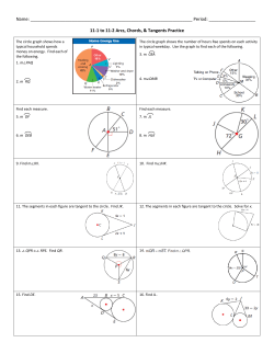


© Copyright 2026