
The Right Type of Legislator: A Theory of Taxation and Representation
The Right Type of Legislator: A Theory of Taxation and Representation∗ Andrea Mattozzi European University Institute and MOVE [email protected] apps.eui.eu/Personal/Amattozzi/ Erik Snowberg California Institute of Technology and NBER [email protected] www.hss.caltech.edu/∼snowberg/ June 2, 2015 Abstract Theories of taxation conclude that legislators’ ability to target redistribution to their districts results in higher government spending and taxation. Yet, despite the fact that securing “pork” is an important part of a legislator’s job in the U.S., but not in European countries, the U.S. has lower taxes. Our analysis adds a simple assumption to standard models to reconcile them with this fact. Our assumption—that those who are successful in the private sector will also tend to be successful in negotiating transfers for their district—allows our theory to match stylized facts about class representation in legislatures. The model can then be used to examine policies aimed at increasing descriptive representation in legislatures. We find that many of these policies have no, or negative, effects on descriptive representation, including: increasing the number of representatives, allowing parties to choose candidates, or giving parties some ability to discipline legislator’s votes and screen candidates. On the other hand, two policies are found to be particularly effective for increasing descriptive representation: proportional representation and limiting competition between legislators. JEL Classifications: D02, D63, D72, D78, H10, H23 Keywords: Political Economy, Citizen Candidates, Taxation, Redistribution, Representation, Legislatures ∗ We thank Jonathan Chapman for excellent research assistance. Snowberg gratefully acknowledges the support of NSF SES-1156154. We thank Ethan Bueno de Mesquita, Josh Clinton, Stephen Coate, Daniel Diermeier, Tim Feddersen, Patrick Francois, Sean Gailmard, Andrea Galeotti, Alex Hirsch, Morgan Kousser, Kai Konrad, Jenny Mansbridge, Gerard Padr´o i Miquel, Pablo Montagnes, Salvatore Nunnari, Giacomo Ponzetto, Debraj Ray, Jean-Laurent Rosenthal, Allistair Smith, Ken Shotts, Jim Snyder, Francesco Trebbi, Leeat Yariv, and seminar audiences at the Priorat Workshop, the Rotterdam Workshop in Political Economy, WZB Berlin, the Chicago Workshop on Institutional Design, the Collegio Carlo Alberto, MPSA, Caltech, the University of Miami, IPEG, MEDS, George Mason, Georgetown, UBC, and UCB for useful conversations, comments, and encouragement. We also thank the Casa del Popolo di Fiesole for their hospitality, although it may have been reduced had they known what we were writing. 1 Introduction A central question in political science involves the determination of economic policies, like tax regimes. In the seminal models of distributive politics, legislators are viewed as independent actors mainly interested in directing public funds to their district at the expense of the general population (Tullock, 1959; Weingast, 1979; Weingast, Shepsle and Johnsen, 1981). Legislators’ desire to bring “pork” to their districts results in a common pool problem, leading to higher spending, and thus taxation. This mechanism is a fundamental component of the way the existing theoretical literature has modeled fiscal policy outcomes in representative democracies. The main drawback of this approach is that it is exactly the opposite of what is seen across developed countries. In particular, the U.S. has relatively low federal taxes even though successfully delivering pork is an important part of a legislator’s job. In contrast, European countries, such as the U.K., Italy or Germany, have higher taxes yet legislators largely do not compete for pork.1 Further, the literature investigating the empirical relation between the severity of the common pool problem (measured by the size of the legislature) and the size of government is not conclusive, with a number of papers finding a negative relationship.2 In this paper, we reconcile the common pool logic with the above stylized facts, and generate a number of additional testable predictions. We do so by introducing the abilities and personal preferences of legislators into the model. Specifically, we combine workhorse models with a simple assumption: individuals who are more successful in the private sector will tend to be more successful, as legislators, at directing resources back to their district. This assumption is discussed at length in Section 1.3, but it can be easily summarized as: whatever gets one ahead in the private sector—for example: connections, hard work, charisma—is also useful, on average, in negotiating resources for one’s district. We refer to 1 See, for example, http://www.theatlantic.com/business/archive/2013/01/how-low-are-us-taxescompared-to-other-countries/267148/ 2 For a review of the theoretical and empirical literature on the so-called “Law of 1/n” see Primo and Snyder (2008). Pettersson-Lidbom (2012) is one of the cleanest tests, and finds a negative relationship between spending and the number of legislators. 1 these skills, as a group, as negotiating skills. This is in contrast to recent work—reviewed in Section 1.4—that has largely abandoned the common pool mechanism, and instead argues that cross-countries differences in tax regimes are the result of differences in the political system, the electoral rule, or culture. Our results are useful for organizing a number of stylized facts about differences in taxation, redistribution, and representation across developed countries. Our model predicts that the rich will be over-represented in all legislatures. It further concludes that the U.S. will have wealthier legislators, lower taxes, and parties that are less differentiated on tax policy than Western European countries. Further, our model provides an explanation of the underrepresentation of women in the U.S. Congress relative to legislatures in Germany, the U.K., or Italy. Finally, our model is consistent with the discrepancy in the U.S. between the high public approval of individual legislators, and the low approval of the legislature itself. All these predictions are broadly consistent with stylized facts reviewed in Section 9. 1.1 Theoretical Argument Our model allows for redistribution both between the rich and the poor, and between legislative districts. Citizen voting is assumed to follow standard median-voter logic (Hotelling, 1929; Downs, 1957; Meltzer and Richard, 1981). Once elected, legislators participate in a two-stage budgeting process where legislators first vote on taxes using majority rule, and then negotiate over the distribution of the budget (Chari, Jones and Marimon, 1997; Persson, Roland and Tabellini, 1997). Because we assume legislators are citizen candidates, their actions in office follow their own preferences.3 Citizens are one of two types: rich or poor. Our central assumption—discussed at length in Section 1.3—is that the rich have relatively strong negotiating skills, and the poor have relatively weak negotiating skills. The main tradeoff that our model highlights is simple and robust: a district’s legislator, 3 This is in implicit in the citizen-candidate framework of Osborne and Slivinski (1996) and Besley and Coate (1997), and can be relaxed. See Sections 4.3, 6.4, and 10. This is consistent with the selection model of Miller and Stokes (1963), especially as elucidated by Mansbridge (2009). A focus on candidate preferences is rationalizable: Fearon (1999) finds that voters are better off using elections to select types, rather than disciplining incumbents. 2 as one of many in the legislature, has little impact on broad policies, such as the tax rate, but a relatively large impact on the transfers that the district receives. Knowing this, even the median voter of a poor district will ignore a candidate’s preferences over redistribution and focus on his negotiating skills, that is, a rich candidate’s superior ability to direct transfers to his district.4 A more subtle intuition comes from seeing the game that voters play as a prisoner’s dilemma: all poor voters voting for poor legislators would make all poor voters better off. However, it is strictly dominant for an individual poor voter to choose a successful—that is, rich—legislator. This model yields a striking result: when securing resources for one’s district is important, then, in equilibrium, every district votes for candidates who are successful in the private sector—that is, rich. This occurs even though those candidates prefer lower taxes— which they actualize—than voters, and despite the fact that everyone elects equally effective negotiators, so the spending in all districts is equal. The equilibrium exhibits three patterns of representation. When ability to direct funds to a legislator’s own district does not matter at all—say through budgeting procedures that make it impossible to target funding—then every district elects a legislator who is the same type as its median voter, and the tax rate is effectively set by the median voter of the median district. We call this a representative equilibrium. If, instead, ability to direct funds matters just a little, many districts with poor median voters will elect rich legislators. However, poor legislators will still form a minimal winning coalition in the legislature. Those that vote for rich legislators will know, in equilibrium, that they will not cause the legislature to tip to a rich majority, and hence will choose a rich legislator for his superior negotiating abilities. The legislative majority, composed of poor legislators, knows that rich legislators will get more than an equal share of tax revenues, and will shade down the tax rate to reduce the expropriation from their districts. We call such equilibria somewhat representative. Finally, when the ability to direct funds to a legislator’s own district is important, then the unique equilibrium will be for every district to elect a rich 4 We follow the principal-agent literature in referring to legislators (agents) using masculine pronouns, and citizens (principals)—especially the median voter of a district—using feminine pronouns. 3 legislator. This unrepresentative equilibrium occurs due to the logic laid out above. 1.2 Descriptive Representation An attractive feature of our model is that it makes predictions about descriptive representation (which we often refer to simply as “representation” where it will not cause confusion), a subject that has been largely overlooked by formal modelers in favor of ideological representation. However, it is worth noting that our model is only a first step, and thus restricted to descriptive characteristics that bear on representatives’ ability to negotiate resources for their districts—the set of “negotiating skills” we define above. This likely excludes descriptive characteristics that may be of interest to voters, such as ethnicity or religion. Interestingly, many factors that might be thought to be helpful in fostering representation are in fact ineffective or counter-productive. Dahl and Tufte (1973), among others, argue that larger legislatures should promote representation. Unexpectedly, smaller legislative districts, such that each legislator represents fewer citizens, lead to less representative outcomes. Likewise, stronger parties are often seen as a force for increasing representation (Committee on Political Parties, 1950; Hazan and Rahat, 2010). However, in our model, policy-motivated parties with complete control of candidate nomination and some ability to discipline their politicians often make outcomes less representative. The intuition behind these results builds on the logic above. As legislatures grow to include more representatives, each legislator’s influence over broad policy outcomes—like taxation—diminishes, while the influence he has on his own district’s welfare through transfers stays relatively constant. This leads to unrepresentative equilibria even when the rich have a relatively small advantage in directing resources to their own district. Additionally, the ability of policy-motivated parties to discipline their politicians will be used by the party that favors low taxes to make their candidates’ positions on tax policy more attractive to the poor. This, combined with the greater skill of the rich in negotiating transfers for their districts, will lead to all districts electing rich candidates—and these candidates implementing lower taxes than would otherwise be obtained in equilibrium. On the other hand, we 4 show that two factors unambiguously increase representation: proportional representation, and limiting the competition between legislators for district-specific transfers. In addition to the predictions on class representation described above, our model can be extended to any group that is perceived by society as being less able negotiators. A particularly interesting case is women, who are generally perceived as less capable negotiators (Niederle and Vesterlund, 2008; Croson and Gneezy, 2009) or as having less bargaining power than men (Ayres and Siegelman, 1995; Altonji and Black, 1999; Harding, Rosenthal and Sirmans, 2003). Regardless of the correctness of these beliefs—and recent research indicates that they may be mistaken (Volden, Wiseman and Wittmer, 2013; Besley et al., 2014)— our model makes the same predictions for the representation of men as it does for the rich because voters believe that representatives with these descriptive characteristics will be able to deliver more pork to their districts. In particular, men will be over-represented in all legislatures, and legislatures characterized by a focus on pork will have an even greater majority of men than those that are not. Again, these patterns are broadly consistent with the stylized facts described in Section 9. 1.3 Discussion of our Central Assumption The main assumption of our model is that those who are more successful in the private sector are also better at negotiating resources for their district.5 Unfortunately, a direct test of this assumption is hardly feasible because it involves assessing several variables that are often unmeasured, or unmeasurable.6 However, what is actually required is that voters believe this is the case. While this appears plausible prima facie, in order to assess it, we ran a few simple surveys on convenience samples.7 The questions on this survey were aimed at ascertaining whether U.S. voters saw private sector success as a signal of distributive 5 Note that allowing for positive but imperfect correlation between tax preferences and legislative ability can be easily incorporated in our model. See Section BLA. 6 We thank Salvatore Nunnari for pointing out that wealthier legislators, as determined by the poor quality data on opensecrets.org, sponsor more bills, and Jim Snyder for pointing out that Democrats from more marginal districts are more likely to be on one of the “Big 4” committees, where most pork originates. 7 We obtained our convenience samples in the U.S. through Amazon’s Mechanical Turk. For more on the use of Mechanical Turk in survey research see Berinsky, Huber and Lenz (2012). 5 prowess, and furthermore, whether this prowess was enough to overwhelm policy concerns in voting decisions. We asked a sample of U.S. citizens (n = 1, 076) to rank various professions in terms of the respondent’s belief as to which would be most indicative of talent at “obtaining resources for your district (for example by obtaining funding for local projects)”. Respondents ranked a list of professions from 1–6. These professions, with their average rank were as follows: successful businessman (2.07), entrepreneur (2.38), successful lawyer (2.63), high school teacher (3.73), factory worker (4.73), and bus driver (5.46). We also asked the same respondents to rank people with different educational backgrounds in terms of their ability to secure funds for the voter’s district. The rankings were: MBA (2.28), law degree (2.44), PhD (2.78), medical degree (3.83), university degree (4.16), and only high school degree (5.50).8 A clear pattern emerges in this data: more highly compensated professions, and educational backgrounds correlated with compensation, are perceived by voters as being indicative of the legislative skill of directing resources to a district. Finally, we asked a subset of this group (n = 233) a question aimed at understanding how they valued the trade-off between policy and directing resources to their district. We asked them to choose (hypothetically) between a Congressional candidate that was “good at securing resources for your district: he has a long record of bringing in money for projects the district needs and prefers lower taxes, especially on high-income earners”, and another that was “not very good at securing resources for your district and prefers higher taxes, especially on high-income earners”, which one would they choose? The first candidate was chosen by 73% of respondents. Self-identified Republicans chose the first candidate 93% of the time, versus 70% for self-identified Democrats. While this is supportive of the core assumption of our model, for this to have implications for fiscal policy, it must also be the case that the core assumption of the citizen candidate model holds as well. In particular, wealthier legislators prefer lower taxes. Here, we refer to Carnes (2013), which shows, based on roll-call votes, that legislators from higher socio8 All differences between rankings were significant at the p < 0.01 level. The rankings of those who reported they voted in the last congressional election were not significantly different than those who did not. 6 economic status professions have more conservative voting records, even controlling for party. 1.4 Literature Our work is closely related to papers in two additional literatures: the examination of heterogeneity in political skills, and the debate over whether their is a wealth bias—that is, policy follows the preferences of the upper-classes—in U.S. politics. A large literature has developed trying to understand the causes and consequences of “valence” or “quality” of politicians, following Stokes’s (1963) influential critique of the Downsian model. Theory papers of this ilk tend to assume that the valence of a politician is a draw from a distribution (for example, Groseclose, 2001), while empirical papers consider education or prior income as markers of quality (for example, Gagliarducci and Nannicini, 2013).9 Instead, we consider a specific ability—the ability to negotiate resources for their district—and assume that this ability is correlated with private sector success.10 Our paper thus follows an emerging literature that considers additional dimensions of politician heterogeneity.11 Moreover, we explicitly consider the interaction between different legislative districts, and how this alters voters’ preferences over politicians, whereas much of the previous literature considers a single politician in isolation. Our paper also contributes to the debate about whether or not there is a wealth bias in U.S. politics (Bartels, 2007; Gilens and Page, 2014). We build on Carnes’s (2013) empirical findings with a formal-theoretic basis for why poorer voters would choose to be represented by wealthy legislators with policy preferences that differ from theirs. Our explanation is complementary to explanations that focus on differences in campaign resources (Campante, 2011) and the sensitivity of poor voters to the outcomes of richer voters (Bartels, 2007).12 9 Recent research has focused on identifying more direct measures of quality, see, for example Volden and Wiseman (2014). 10 Appendix B.2 compares results with a model where those that are successful in the private sector have a generic ability to improve the efficiency of policy. 11 Besley and Coate (1997) note the tension between politicians’ preferences and their ability to implement certain policies. Other papers in this literature, which often focuses on why poor quality politicians are elected, include Caselli and Morelli (2004), Messner and Polborn (2004), Mattozzi and Merlo (2008). 12 In a related analysis, Bai and Lagunoff (2013) explore what data would be needed to uncover a wealth bias in politics. 7 As mentioned earlier, there is a large literature, reviewed in Persson and Tabellini (2000), that argues that cross-country differences in tax regimes are primarily caused by the electoral system or rule. While these explanations capture important aspects of variation in tax regimes for countries with markedly different systems and rules, such as U.S. and Italy, they are less compelling for countries that are relatively similar, such as the U.S. and U.K. There is also a small literature that explores how experiences and social structure affect voters’ beliefs and preferences over redistribution (Piketty, 1995; Alesina and Angeletos, 2005). Our paper instead focuses on the preferences of legislators. However, additional value may come from examining the belief formation process of legislators, and how this may in turn affect their reaction to informational lobbying. Finally, in both the somewhat representative and unrepresentative equilibria of our model, poor voters will vote for rich candidates who prefer a low tax rate. Huber and Ting (2013) also explain this behavior, although their explanation relies on parties that can exclude legislators from the opposing party from receiving funds. The poor then vote for the rich party in order to avoid being in the legislative majority. It is worth noting that this relies on powers there is little evidence that parties have: heterogeneity in federal spending across districts is not well explained by the party of the legislator (Boone, Dube and Kaplan, 2014). Moreover, coordination could be either on the party of the rich or the party of the poor. 2 Model In this section we lay out our core model. We then build intuition for our results by analyzing a simplified version with only three legislative districts. 2.1 Structure and Players Legislative Districts We model a country populated with a unit measure of citizens, and with 2n + 1 legislative districts j ∈ J = {1, 2, . . . , 2n + 1}, each containing an equal measure of citizens. 8 Citizens: A citizen’s utility is her post-tax income plus utility from government spending in her district. A citizen’s pre-tax income is determined solely by her publicly observable type, t ∈ {l, h}, which is either low or high. Specifically, the income of a low type is yl , and the income of a high type is yh = ηyl , with η ∈ (1, η) parameterizing the productivity difference between high types and low types. We occasionally refer to high types as rich or successful, and low types as poor or unsuccessful. Overall, a fraction λ of citizens are low types, so the total income of all legislative districts together is given by y ≡ (λ + (1 − λ)η)yl . We restrict the tax instrument τ to be linear in income, so tax revenue is given by τ y.13 j District j receives a proportion π−j of tax revenues, which is determined by the type of legislator elected in j’s district, as well as the other (−j) districts. Section 2.2.2 describes the specific process determining this distribution. The utility that each individual receives from x amount of local government spending is g(x) = xα /α with α ∈ (0, 1). Given the above, we can write the utility of an individual voter as: α j τy π−j . uij = (1 − τ )y + α i (1) j When an equal proportion of tax revenues is transferred to each district π−j = 1/(2n+1), and we denote by τl∗ and τh∗ the most-preferred tax rates of low and high types, respectively: τl∗ = α !1−α y 1 α (2n + 1)yl and τh∗ = α !1−α y (2n + 1)(ηyl ) 1 α τl∗ = η 1 1−α < τl∗ . (2) To guarantee τl∗ < 1, we assume that (2n + 1)yl > y α . Finally, we denote by ul (τ ) the utility a low type receives from a given tax rate τ when tax revenues are divided equally between districts. Legislators: Legislators are citizen candidates, implying that their actions in office are determined solely by their preferences as citizens. Initially, we assume that two candidates run in each district, a low type and a high type. Later, we endogenize candidate selection 13 Section 10 briefly discusses more complicated tax instruments. 9 by adding parties. As types are publicly known, voters know what each candidate will do if elected, and vote accordingly. Median Voters: Using standard results, the winning candidate will be chosen by the median voter of each district. A number z ≡ b(1 − λ)(2n + 1)c ∈ {0, 1, . . . , n} of districts have a high-type median voter. By making the proportion of high-type median voters roughly equivalent to the proportion of high types in the population, we eliminate the effect of the boundaries of districts on representation (Chen and Rodden, 2013). 2.2 Timeline Our model of elections and legislative policymaking proceeds in three stages. These are: 1. The voting stage. Voters simultaneously vote for one of two citizen candidates based on the utility they expect to receive with each candidate as their representative in the legislature. Thus, their votes will depend on the candidates’ types, and the types of candidates elected by the other legislative districts. 2. The tax-policy stage. Legislators vote on a level of taxes using an open rule. In subgame perfect equilibria, legislators will take into account what will happen in the distributive stage. As the majority of the legislature will always be of the same type, they will have the same most-preferred tax rate, which will be adopted. 3. The distributive stage. Distribution of the public budget among the three districts is determined by a negotiating process described in Section 2.2.2. After the distribution stage, incomes are realized, taxes are levied, and tax revenue is distributed according to the decisions described above. 2.2.1 The Voting and Tax-Policy Stages The first two stages are governed by standard median voter results. Two districts have a low-type median voter, and one a high-type median voter. In the tax-policy stage, tax 10 preferences will depend on a legislator’s type, and the type of the other legislators. However, there will always be at least n + 1 legislators who are the same type—and face the same other types in the legislature—and thus will end up with the same most-preferred tax rate. These legislators will vote together to establish the tax rate. 2.2.2 The Distributive Stage The third, distributive, stage ties together productivity in the public and private sector, and contains the assumption crucial for our results. As noted above, each district receives public transfers funded by a linear tax on income. High types are advantaged in negotiating transfers for their district by the same proportion as their increase in productivity in the private sector: η. Section 4.3 discusses the case when negotiating ability and preferences for redistribution are imperfectly correlated. A high type’s advantage may be mitigated by institutional features. In particular, 1−γ ∈ [0, 1] parameterizes the degree to which a high type’s negotiating ability is restricted.14 The proportion of tax revenues that a district receives takes on six values that are relevant for the analysis. We define these as: L π(2n+1)L = L π(n+1)L = 1 n((1−γ)+γη)+(n+1) L π(n+1)H 1 (n+1)((1−γ)+γη)+n 1 , 2n+1 < 1 , 2n+1 H π(n+1)L = (1−γ)+γη n((1−γ)+γη)+(n+1) < 1 , 2n+1 H π(n+1)H (1−γ)+γη (n+1)((1−γ)+γη)+n > 1 , 2n+1 > 1 , 2n+1 (3) = H and π(2n+1)H = = 1 , 2n+1 where the subscript displays the number and type of legislators in the legislative majority, 14 Formally, the share of tax revenue that is returned to district j is given by: ( (1−γ)+γ∗1 P i if legislator j is a low type is sj = (1−γ)+γ∗η P i if legislator j is a high type, s i This particular form can be motivated by the Baron and Ferejohn (1989) legislative bargaining model, see Appendix B.4. However, modeling this explicitly makes outcomes risky from the perspective of the voter, which, given the concavity of the utility of public spending, will lead to effects that obscure the main intuition driving our result without qualitatively affecting it. 11 and the superscript defines whether district j is represented by a high-type or low-type legislator. Note that the denominator changes to ensure that the sum of proportions always equals one. The existence of different abilities in negotiating transfers for a legislator’s district is the major way in which our model departs from previous work. The parameter γ dictates the extent to which negotiating ability will matter for the transfers to a legislator’s district. If γ is low, then most funds are simply divided evenly between districts, and a legislator’s type will matter very little for the amount of transfers a district will receive. On the other hand, when γ is high, a legislator’s type may matter quite a lot. Thus, 1 − γ can be thought of as any institutional features that limit the competition between legislators, or reduce the amount of tax revenue a high-type legislator can negotiate for his district. For example, the ability to target only to broad demographic groups, rather than to narrow geographic areas, would result in a lower γ. How institutional features shape γ and the nature of representation is the subject of extensive discussion in Sections 6 and 7. 2.3 Equilibrium We focus on subgame perfect equilibria, and establish an equilibrium concept, stage-strong, to judge the robustness of equilibria to coordinated deviations of multiple legislative districts. Definition 1. An equilibrium is a pure-strategy, subgame-perfect Nash equilibrium in which voters play weakly-undominated strategies. A stage-strong equilibrium is an equilibrium where there are no joint deviations within a single stage of the game that make all deviating players weakly better off, and one player strictly better off.15 The assumption that voters play weakly-undominated strategies means we can just examine the strategies of the median voters of each district. The equilibria of this model can 15 In our environment, there will be no strong Nash equilibria, but the deviations that prevent such equilibria from occurring are not sequentially rational. On the other hand, unique equilibria are always coalitionproof (Bernheim, Peleg and Whinston, 1987; Bernheim and Whinston, 1987). Stage-strong equilibria are thus more robust to deviations than coalition-proof equilibria, but impose that deviations be sequentially rational. 12 be of three types. To fix terminology, we define: Definition 2. 1. We say an equilibrium is representative if the tax rate is the same as the most preferred tax rate of the median voter of the median district, τl∗ . 2. We say an equilibrium is somewhat representative if there is an over-representation of high-types in the legislature, and the equilibrium tax rate is τ ∈ (τh∗ , τl∗ ). 3. We say an equilibrium is unrepresentative if all districts elect high-type legislators, and the tax rate is that most preferred by a high-type citizen, τh∗ .16 3 Central Result Here we state our central result, before building intuition using the case with three legislative districts (n = 1). The result shows that when legislators’ ability to negotiate spending for their district does not matter, fairly standard results apply. However, when this ability is important, no district wants to reduce their transfers by electing a low-type legislator, and thus, only high-type legislators will be elected in equilibrium. Because high-type legislators are richer, they have a personal preference for lower taxation, which determines the equilibrium level of redistribution. Proposition 1. 1. If γ = 0, then every equilibrium is representative with tax rate τl∗ , and all districts receive an equal proportion of the tax revenues. 2. If 0 < γ < γ ∗ (n) < 1 there are two types of equilibria: (a) Unrepresentative equilibria, with the legislature composed of all high types, and tax rate τh∗ . These equilibria are not stage strong. (b) Somewhat representative, with the legislature composed of n + 1 low types and n α L ∗ 1−α high types, and tax rate ((2n + 1)π(n+1)L ) τl < τl∗ . 1−α 1 1−α α z 1 ∗ 3. If γ (n) < γ < 1 then the unique equilibrium is unrepresentative. If 2n+1 > γ(η−1) η α η−α −1 this equilibrium is stage strong. 16 We do not conduct welfare analyses, as these depend critically on assumptions about the distortionary effects of taxation. That is, there exists some level of distortion such that any of these equilibria structures may be welfare maximizing. 13 Figure 1: Equilibrium structure depends on the value of γ. The quantity γ ∗ (n) is defined implicitly. In particular, γ < γ ∗ (n) ⇐⇒ H π(n+1)H L π(n+1)L α !1−α < ul (τl∗ ) − yl ul (τh∗ ) − yl (4) which is important in the following analyses. Before turning to a detailed construction of this result, note that the money transferred to each district will always be relatively equal. In the representative equilibrium, transfers are equal because γ = 0. In the unrepresentative equilibrium, all districts elect high types, leading to equal transfers. In the somewhat representative equilibria, transfers may be unequal, but they will be similar, as these equilibria only obtain for low values of γ, which is when high types have the smallest advantage in negotiating transfers for their districts. 4 Example: Three Districts To elucidate the central role that negotiating ability plays in our results, and build the intuition behind Proposition 1, we first examine the case when n = 1, that is, when there are three legislative districts. This example will also allow us to understand the case when tax preferences and negotiating ability may be imperfectly correlated. 4.1 Representative Equilibrium 14 L H L H When γ = 0, then (3) simplifies to π3L = π2L = π2L = π2H = π2H = π3H = 1/3. That is, no matter what type of legislator a district elects, it will receive the exact same amount of the tax revenue. Thus, the median voter of each district will focus on the effect that her legislator will have on the tax rate. As such, median voters choose to elect someone who favors exactly the same tax rate that they do. The more interesting cases are the stage-strong equilibria when γ > 0. As the equilibria we consider are subgame perfect, we can solve for them using backwards induction. 4.2 Building the Central Result with Imperfect Discipline When γ > 0 there is the potential for redistribution not just between rich and poor, but also between districts. This changes incentives, especially for low-type median voters. If both of the other districts are electing a high type, a low-type median voter will want to elect a high type as well, leading to the first equilibrium in Part 2 of Proposition 1. However, this equilibrium is not stage strong. Specifically, if two districts with low-type median voters deviated to elect low-type legislators, these districts would be strictly better off. When γ < γ ∗ (n) holds, this deviation is also an equilibrium, and it is stage strong. However, when γ > γ ∗ (n), then this cannot be sustained as an equilibrium, as each low-type median voter is made strictly better off by electing a high type, no matter who the other median voter elects. 4.2.1 The Legislative Stages The outcome of the distributive stage is determined by the types of the three legislators, according to (3). As we focus on subgame perfect equilibria, the legislators will take this expected distribution into account when voting on the tax rate. If the legislature is composed either entirely of high types or entirely of low types, then all three districts will receive the ∗ ∗ same proportion of tax revenue πj = 1/3 for all j. Thus, τ3L = τl∗ , and τ3H = τh∗ , which are the ideal tax rates of high- and low-type citizens, respectively. The legislative majority could also consist of two low types or two high types, which leads to two other potential values of 15 Table 1: Median Voter Incentives If the other two districts elect A low-type median voter will want to elect a A high-type median voter will want to elect a Two low types: high type high type A low type and a high type: low type if: α H 1−α π2H ul (τl∗ ) − yl ≤ , (5) L ul (τh∗ ) − yl π2L high type otherwise, a high type Two high types: high type high type the tax rate in equilibrium, α ∗ L 1−α ∗ τ2L ≡ (3π2L ) τl and α ∗ H 1−α ∗ τ2H ≡ (3π2H ) τh , (5) L H L H ∗ ∗ = 13 , τ2L = 13 , τ2H < π3L > π3H > τh∗ , and as π2L < τl∗ . Thus, respectively. Note that as π2H ∗ ∗ in equilibrium, τl∗ < τ2L < τ2H < τh∗ . 4.2.2 The Election Stage The utility of a median voter in a given district will depend on the types of the legislators elected from all three districts (see (3) and (5)). It is thus useful to examine what type of legislator a median voter would want to elect given the types of legislators elected from the other two districts. As, in equilibrium, a voter’s beliefs about the types of the legislators elected by other districts must be correct, these preferences will shape the median voter’s vote choice. The preferences of median voters, conditional on the types elected in other districts, are 16 summarized in Table 1. A high-type median voter will always want to elect a high type, as, from her perspective, there is no strategic delegation problem. A low-type median voter will also want to elect a high-type legislator whenever the other two legislative districts both elect high types or both elect low types, as the median voter’s choice will not affect tax rates much, and they will get a larger portion of tax revenue. The crucial conflict occurs when a low-type median voter is pivotal in determining the majority type in the legislature. In this case, she must weigh the benefits of a high type’s ability to direct resources to her district—the left-hand side of (5)—against the cost of allowing high types to set the tax rate—the right-hand side of (5). This inequality is the same as (4) for n = 1, and is crucial in understanding the unrepresentative equilibrium. When it fails to hold, a low-type median voter will not want to elect a low-type legislator, even when she knows her choice will be pivotal in determining the majority type in the legislature. Thus, two districts with low-type median voters are in a prisoner’s dilemma: they cannot commit to each other to both elect low types—even if one followed through, the other would be strictly better off electing a high type. 4.3 Imperfect Correlation between Types There are, of course, politicians who are successful in the private sector, but favor high taxes. Allowing for positive but imperfect correlation between tax preferences and legislative ability can be easily incorporated in our model as long as we maintain our assumption that the only signal of a citizen’s type is his or her success. In this case, there is little effect on our results, and the existence of such a correlation may make unrepresentative equilibria hold for a wider range of parameter values—that is, it may lower γ ∗ (n). In particular, consider the case where success in the private sector is a perfect signal of a citizen’s ability to direct resources to his district, but an imperfect signal of his tax preferences. That is, with probability 1 − q < 1/2 a high-type citizen will vote for tax rates as if he had low income, yl . This means that ability to direct funds to one’s district and tax preferences are imperfectly correlated (with a correlation proportional to q), and there is a 17 single signal of both dimensions of a citizen’s type. When private-sector success is imperfectly correlated with tax preferences, (4) becomes: H π2H L π2L H π2H L π2L α 1−α ≤ ul (τl∗ ) − yl q2u α 1−α ≤ ∗ l (τh ) + (1 − q)2 ul (τl∗ ) + 2q(1 − q)ul ul (τl∗ ) − yl q(2 − q)ul (τh∗ ) + (1 − q)2 ul (τl∗ ) − yl τl∗ when γ is low α ((1−γ)+γη) 1−α − yl when γ is high. The difference in expressions is due to the fact that when two districts elect high types, as γ grows, the identity of the median voter changes from a low type to a high type. Proposition 2. γ ∗ (n) is increasing in q. That is, the higher the correlation between the different dimensions of a citizen’s type, the broader the range of parameters for which a somewhat unrepresentative equilibrium occurs. To see why, note that the denominator of the right-hand side is larger when private sector success is an imperfect signal of tax preferences. Intuitively, the cost to a low-type median voter of electing a high type is reduced because the high type might share the low type’s preferences for redistribution.17 5 The Common Pool As pointed out in the introduction, a central question in the literature on fiscal policy is how taxing and spending evolve as the size of the legislature grows. In this respect, our model delivers an anti-common pool result, which appears to be consistent with a number of empirical findings.18 To establish this, we examine how taxing and spending evolve as n, and thus the size of the legislature, grows. The main mechanism at work here is that as n 17 Note that the probability that these high types with preferences for large amounts of redistribution will be numerous enough to affect the tax rate (that is, a majority of the legislators) will be less in larger legislatures. Moreover, as the legislature grows, the number of high types in the somewhat representative equilibria may be a super-majority, without composing the entire legislature, as the biggest change in utility between electing a high and a low type may occur in a district other than the median. This complexity accounts for the fact that we chose to display this result, which holds in general, for the case of n = 1. 18 See the review in Primo and Snyder (2008). 18 grows, the effect of a legislator’s ability to negotiate resources for his district is relatively constant, while his effect on tax policy shrinks. As such, low types want to elect high-type legislators even if γ is relatively low. Recall that there are z ≤ n high-type median voters. These voters will always elect a high-type legislator. Thus, when (4) holds, n − z low-type median voters will elect high-type legislators. This makes the remaining n + 1 low-type median voters pivotal, so they will prefer to elect a low-type legislator. On the other-hand, if (4) does not hold, then low-type median voters always wish to elect high-type legislators, no matter who is elected in every other district. As electing a low-type legislator is strictly dominated, the unique equilibrium will be for every district to elect a high-type legislator. To understand how (4) depends on n, note that the right-hand side can be reduced to 1 η 1−α (1−α) η−α , which is constant in n. However, the left-hand side is increasing in n. Thus, holding γ > 0 constant, as n grows there is a point where the equilibrium switches from a somewhat representative equilibrium to the unrepresentative equilibrium. Defining τn∗ as the tax rate implemented when there are 2n + 1 legislators, the next result makes this point precise: Proposition 3. 1. γ ∗ (n) is decreasing in n. As n → ∞, γ ∗ (n) → κ(η, α), where κ(η, α) ∈ (0, 1). 2. τn∗ is decreasing in n.19 There are two reasons that taxes decrease when n increases. First, the tax rate in a α L somewhat representative equilibrium is ((2n + 1)π(n+1)L ) 1−α τl∗ . This is decreasing in n, due to the fact that as n increases, closer and closer to 50% of the districts are represented by high types. Thus, if γ < κ(η, α) then the tax rate be will continually decreasing as n grows. ∗ On the other hand, if γ > κ(η, α) then at some n the tax rate will drop from τ(n+1)L > τh∗ 19 This is due, in part, to the way we have modeled the utility of government spending: the functional form implies spending is on local public goods. Thus, as districts become smaller, the effectiveness of this spending goes down (see, for example, the expression for τl∗ in (2)). Appendix B.5 shows the result still holds when using a slightly different citizen utility function that does not have this feature. 19 Figure 2: The Anti-Common Pool: Tax rates decrease with n. (a) γ is small. (b) γ is large. to τh∗ as the equilibrium moves from somewhat representative to representative.20 As n grows beyond this point, the tax rate will be τh∗ . Thus, the tax rate will either be smoothly decreasing in n, or will decrease smoothly in n up until a point when the equilibrium switches from somewhat representative to unrepresentative, at which point there will be a sudden decrease in the tax rate. 6 Policies that do not Increase Descriptive Representation In this section and the next, we examine how various features of a political system interact with descriptive representation. This shift away from direct policy implications allows us to produce novel results that can apply to any group perceived as being less skilled at negotiating (for example, women, see Section 1.2). As noted in that subsection, we will often shorten “descriptive representation” to just “representation” when it is unlikely to cause confusion. We find that increasing the number of representatives, allowing policy-motivated parties 20 ∗ When γ and η are particularly large, it may be the case that τ(n+1)L < τh∗ , as much of the tax revenue will go to the high-type legislator’s district. Anticipating the outcome of the distributive stage, a majority composed of low-type legislators will set a relatively low tax rate in the tax-policy stage to prevent their ∗ districts from being expropriated. Similarly, it may be the case that τ(n+1)H > τl∗ . While these orderings are theoretically possible, they never obtain in equilibrium. 20 to control representation, discipline legislators, or screen candidates, has little effect on representation, and may, in fact, reduce representation. On the other hand, in the next section, we find that representation is improved by proportional representation, and parties (or other institutional features) regulating competition between legislators. To formally analyze representation, we define: Definition 3. The index of (descriptive) representation is ξ≡ # of low-type legislators . # of districts with low-type median voters As we are also interested in the effect of these possible reforms on the representation of women in the legislatures, with proper modification, this definition can be seen as applying to either class or gender. 6.1 Increasing the Number of Representatives In a series of articles appearing in the online edition of the New York Times, a number of commentators argue in favor of increasing the size of state legislatures, and enlarging the House of Representatives.21 In the academic literature, Dahl and Tufte (1973) argues that larger legislatures should promote representation of minorities, and Taagepera and Shugart (1989) suggests that states with small legislatures (in particular smaller than the cube root of their population size) cannot achieve representational goals. Furthermore, the National Conference of State Legislatures argues that smaller legislative districts are preferable as, “The legislature is designed to provide a cross-section of all points of view.” 22 Paradoxically, more representatives leads to less representative equilibria. Corollary 4. If γ > 0, ξ is decreasing in n. 21 http://economix.blogs.nytimes.com/2013/12/31/the-size-of-state-legislatures; http://economix.blogs.nytimes.com/2014/01/07/enlarging-the-house-of-representatives; http://www.nytimes.com/2011/01/24/opinion/24conley.html 22 http://www.ncsl.org/research/about-state-legislatures/sizes-of-legislatures.aspx 21 If γ > 0, no equilibria will be representative except in the case when n = 0. As n increases, representation will decrease. This is a direct corollary of Proposition 3. 6.2 Party Control of Candidate Nominations Hazan and Rahat (2010) argues that more exclusive and centralized methods for selecting candidates will increase representation. We can theoretically examine this argument by adding two policy-motivated parties that simultaneously nominate a slate 2n + 1 citizen candidates, one for each legislative district.23 These slates are announced before the election stage (see Section 2.2). That is, there is a closed list. The two parties are L—the party of labor, which has a preference for high tax rates—and H—the party of hoity-toity citizens, which has a preference for low tax rates. If the tax rate chosen by the legislature is τ ∗ , then the utility of the two parties is: UL = fL (|τ ∗ − τl |) UH = fH (|τ ∗ − τh |) we assume each fj is strictly decreasing, so is maximized when τ ∗ = τj∗ . Proposition 5. 1. If 0 < γ < γ ∗ (n) < 1 then party L nominates at least n + 1 low-type candidates in districts with low-type median voters, and is otherwise indifferent. Party H nominates n high-type candidates, and is otherwise indifferent. 2. If γ ∗ (n) < γ < 1 then party H nominates high-type candidates in every district. Party L is indifferent in all districts. 3. All patterns of representation and taxation continue to hold as in Proposition 1. The patterns of nomination may seem somewhat odd. However, if we eliminate weakly dominated strategies, then each party would only nominate citizens of its type. This leads to exactly the same slate of candidates assumed in the setup for Proposition 1, and thus the patterns there will trivially hold. The intuition behind all of these results is that although the low party can supply low-type candidates in each district, this will not change the type for 23 If parties value winning even very slightly, then Downsian logic holds, and both parties will want to nominate whoever voters want to elect. As such, the equilibrium patterns in Proposition 1 hold trivially. 22 whom voters want to vote. If the median voter of a district wants to elect a high type, then the high party is more than happy to supply one as a candidate. As such, the introduction of parties with perfect control over nomination does not affect representation, ξ. There is one difference in the logic between this proposition and Proposition 1: when γ < γ ∗ (n) the reason the unrepresentative equilibrium is not stage strong is slightly different. To support the unrepresentative equilibrium, both parties must nominate high types in all districts. For this to be the case, the low party must believe that if it nominates low types in districts with low-type median voters, then all districts would still elect high types. As this is a subgame-perfect equilibrium of the continuation subgame, it is an equilibrium. However, this continuation play is not stage strong: in particular, if the low party nominated low types, a deviation in the election stage by n + 1 districts with low-type median voters would make them both strictly better off. As such, the unrepresentative equilibrium is not stage strong when (4) holds. 6.3 Party Discipline Suppose, in addition to closed list nominations, parties can somehow discipline their legislators to adopt tax rates other than those they most prefer. That is, they can promise voters that politicians from their party, if elected, will vote for a tax rate that is (at most) ∆τ away from the legislator’s ideal tax rate. This is a reduced form of a model in which parties have only an imperfect ability to discipline their politicians once in government. Parties’ ability to discipline legislators will never increase representation. However, in two circumstances it can increase the tax rate. The first is when the equilibrium is unrepresentative. In this case, high-type candidates from the party L can be forced to implement a higher tax rate. Second, if ∆τ is large enough then any equilibrium will approximate a representative equilibrium—that is ∆τ ≈ τl∗ − τh∗ . In between these circumstances are values of ∆τ for which the ability of parties to discipline their legislators leads to lower tax rates and decreases ξ. 23 Proposition 6. If 0 < γ < γ ∗ (n), then there exists some ∆∗τ such that when ∆τ ∈ ∗ − τh∗ ) then τ ∗ and ξ will be lower in equilibrium when parties can discipline (∆∗τ , τ(n+1)L their legislators than when they cannot. To understand this result, note that when 0 < γ < γ ∗ (n) all stage-strong equilibria are somewhat unrepresentative. Then, consider the lower bound of ∆τ in the proposition. At this level, it will be the high party—not the low party—that will take advantage of the ability to discipline its politicians. Specifically, it will promise that high types elected under its banner will implement a tax rate τh∗ + ∆∗τ , which will be sufficient to change the equilibria from somewhat representative to unrepresentative, thus reducing ξ. Correspondingly the ∗ ∗ tax rate will decrease from from τ(n+1)L to τh∗ + ∆∗τ < τ(n+1)L . The low party will need to respond by also nominating high types and promising a tax rate of τh∗ + ∆∗τ —if it failed to do so then the high party would promise a lower tax rate and win, making the low party strictly worse off.24 Thus, parties with limited ability to discipline politicians may lead to less representative outcomes. 6.4 Parties Can Screen Candidates As in Section 4.3, we assume there exist potential candidates who negotiate like high types, but have the tax preferences of low types. In that section, the proportion of high types that had this property was 1 − q > 1/2. In that section, the presence of such types never increased representation, and may, in fact, may decrease representation because it lowers the (expected) cost to a low-type median voter of voting for a high-type candidate, leading to unrepresentative equilibria. If we suppose that party L has a superior ability to screen for such candidates—that is, they can lower q, the correlation between tax preferences and negotiating ability among their pool of high-type candidates—then this will reinforce the patterns found in Section 4.3. 24 A similar logic applies if parties are able to promise a specific value of γ as long as the low-party cannot promise γ = 0. In Section 8 we consider how changing institutions (γ) affect the long-run play of the game. 24 That is, party L’s ability to screen candidates will decrease representation. 7 Policies that do Increase Descriptive Representation Many factors that might be thought to be helpful for representation have been shown, in our model, to be ineffective or counter-productive. What, then, increases representation? We have identified two factors that unambiguously increase representation: proportional representation, and limiting the competition between legislators for district-specific transfers. After discussing this briefly, we then turn to a dynamic version of our model to examine how changing institutions to limit competition may (or may not) be achieved. 7.1 Proportional Representation Many previous scholars (for example: Boix, 2001; Persson and Tabellini, 2003) have documented a relation between proportional representation (PR) and increased spending. This occurs in our model through increased representation of the poor, rather than through the distributive channels emphasized in previous work (see, for a review, Persson and Tabellini, 2000). In particular, proportional representation is the same as a country having a single district, that is, n = 0. As already shown in Section 6.1, the only value of n for which equilibria will be representative is zero. This occurs because a single district cannot fall prey to the prisoner’s dilemma that reduces representation in other equilibria. To put this another way, a single district takes distributive issues off the table, and allows low types to focus on, and express, their tax preferences. 7.2 Limiting Competition given that we have defined the parameter γ as the amount of competition between legislators to bring resources back to their district, and decreasing γ has already been shown to increase representativeness, it is almost tautological to say that reducing competition will increase 25 representation. But how can this actually be achieved? From Section 6.2, it should be clear that even if a strong party could limit competition, it may not want to, as a relatively even distribution of funds may cause a loss of seats that some targeting of funds would help secure. An example of how γ might actually be lowered comes from Great Britain. In the British parliament, the ability to channel funds to one’s district is severely curtailed. All bills on serious matters such as budgeting must be sponsored by the government (Prime Minister and his or her cabinet). Each year only 20 bills may be sponsored by individual members, in so called private bills. These bills are often quite limited in scope: for example, they may seek to keep a hospital or local center open despite bureaucratic cuts or shifting of resources in an overall program. As we discuss in Section 9, Britain’s system allows for much more representation of the lower classes, despite the fact that it is not a PR system. 8 Changing Institutions: A Mixed Effect This section examines the dynamic incentives to change γ, and finds that the details of institutional change, particularly whether it is slow or fast, are critically important for whether a low level of γ can be achieved and maintained. Under our definition of slow institutional change, γ in the current period is set by the legislature in the previous period. Under fast institutional change, the current legislature is free to set γ before any policy decisions are made.25 We show that when institutional change is slow, the unrepresentative equilibrium will be an absorbing state, whereas the representative or somewhat representative equilibria will not be. That is, the repeated game will eventually get “stuck” in the unrepresentative equilibrium. On the other hand, if institutional change is fast, then the equilibrium in each period will be representative. The asymmetry in “stickiness” of the two types of equilibria, along with the fact that there are no costs to institutional change in our model, present a rare example of fast institutional change perhaps being preferable to slow institutional change. 25 McKelvey and Riezman (1992) studies seniority in legislatures in a similar way. 26 We define a period as a single iteration of our model with three legislative districts (n = 1), as in Section 4. Additionally, we assume that one district always has a high-type median voter (z = 1); we refer to this as the high district. A second district has a small probability, 1 − p, that the median voter there will be a high-type; we refer to this as the middle district. The type of the middle district’s median voter is realized before the voting stage of each period. We also assume that all players have a common discount factor between periods of δ < 1. We focus on Markov-perfect equilibria. To avoid issues of the state variable encoding entire histories, we restrict γ to take on one of two values γ ∈ {0, 1}. The state will thus include the type of the middle district’s median voter, and the value of γ at the beginning of the stage. We begin by presuming that institutional change is slow: the institutional features γ in a given period are set by the previous period’s legislature. We further assume that in the first period γ = 0. Then we have: Proposition 7. 1. If δ < δ ∗ (p) then in each period the Markov-perfect equilibrium will be representative until the first period when the median voter of the middle district is a high type. Thereafter γ = 1, and the equilibrium will be unrepresentative. 2. If δ > δ ∗ (p) then the stage-strong, Markov-perfect equilibrium will be representative if the median voter of the middle district is a low type for at least two periods. The threshold that distinguishes these two types of equilibria depends on the trade-off of low-type median voters when γ = 1. Electing low types in the current period results in a current period loss because low-type legislators will be expropriated by the single high-type legislator. On the other hand, low-type legislators will set γ = 0 for the next period. The value of this policy, however, must be discounted both by δ, and by the probability that the middle district’s median voter will be a high type in the next period (1 − p). When the short-term losses outweigh the long-term gains, low-type median voters prefer to elect high types in the current period. High-type legislators will perpetuate the γ = 1 status quo, and so outcomes will be unrepresentative from then on. 27 Figure 3: Progression of tax rates over time when δ < δ ∗ (p). (a) Slow institutional change leads to permanent unrepresentative equilibria. (b) Fast institutional change allows for representative equilibria. Alternatively, if the current legislature is able to set its own institutional rules, then a low-type median voter will face no conflict between the current period and future periods. In particular, if the majority of the legislature is composed of low types, then they will vote to set γ = 0 in the current period, tax revenues will be equally apportioned, and the tax rate set by the legislature will be the ideal tax rate of a low type. That is: Proposition 8. When institutional change is fast, then equilibria in each period will be representative. Note that there are two reasons why slow institutional change causes less representative outcomes than fast institutional change. First, when policy preferences change, policy will not reflect the desires of voters until institutional change takes place, which happens more slowly. Secondly, and more dramatically, when δ < δ ∗ (p), as soon as a high type is elected in the middle district, he becomes a de facto dictator. If voters are very impatient (δ is low), then even when the median voter of the middle district is (almost) always a low type, the equilibrium will remain in the unrepresentative state, just because once, long ago, the middle district had a high-type median voter. Note that other factors that might slow institutional change will only make this problem worse: if it takes more periods for an institutional change to occur, or super-majority requirements for institutional change, this will only make the unrepresentative equilibrium 28 stickier. That is, Proposition 8 would hold for larger values of δ. Additionally, myopic voters, who act as though their discount rate were 0, would also cause the equilibria to be those identified in Part 1 of Proposition 8. 9 Empirical Regularities As mentioned in the introduction, our results are useful for organizing stylized facts about taxes, redistribution, and representation.26 The analysis of these stylized facts proceeds by noting that the ability to direct funds to one’s district is important in the U.S. (highγ), but is relatively unimportant in most Western European countries (low-γ). Here we focus on three Western European countries—Italy, Germany, and the U.K.—due to the relative ease of obtaining descriptive data from them. While the data in these countries is still imperfect, especially when it comes to legislator wealth, previous scholarship eases constraints somewhat. A full comparative analysis is well beyond the scope of this formaltheory paper. When γ > 0, then the rich will be over-represented in legislatures, as will men. The literature on legislative recruitment concludes, “[T]hat legislatures worldwide include more of the affluent than the less well-off, ... and more white-collar professionals than blue-collar workers” (Norris, 1997, p. 6). Despite the fact that most countries are roughly 50% women, only two countries in the world—Rwanda and Bolivia—have a lower house which is a majority women, and no country in the world has an upper house that is a majority women.27 Other implications require us to compare high- and low-γ countries, as described above. While the rich and men are over-represented in all countries, the over-representation should be particularly extreme in high-γ countries. In countries such as Italy and Germany, about a quarter of legislators have no post-secondary education, and Britain famously has coalminer and factory-worker MPs, while in the U.S., there are almost no legislators who are 26 In order for this to be valid, the assumptions of our model must hold: this is defended in Section 1.3. Oakes and Almquist (1993) reports that the size of the legislature has a very weak effect on representation of women in cross-country regressions. 27 29 laborers or without college degrees (Wessels, 1997; Carnes, 2013). As of April, 2015, of these countries the U.S. had the lowest rate of female representatives in the lower house (19.4%), and Germany the highest (36.5%). The U.S. ranks 73rd in the world, the UK 59th, Italy 33rd, and Germany 20th for female representation. Taxes should be lower in high-γ countries, and, indeed, federal tax rates in the U.S. are lower than in the UK, Italy, or Germany. High-γ countries will also have different party arrangements: specifically, there will be very little difference between the parties in high-γ countries. In the U.S., a change in the party of the President moves the U.S. stock market by ∼ 2%, and a change in the party controlling Congress moves the stock market by ∼0.2% (Snowberg, Wolfers and Zitzewitz, 2007a,b). In contrast, in the UK, a change in the government moves the British stock market by ∼11% (Herron, 2000). Moreover, in high-γ countries, distribution of spending across districts should be independent of the political party of a district’s legislator, and this appears to be the case (Boone, Dube and Kaplan, 2014). High-γ countries should also be composed of higher productivity legislators. While this is difficult to compare in data, we note that members of the U.S. Congress introduce ∼5,000 bills per year, while the Italian Parliament introduces ∼2,000 bills a year, and the UK Parliament introduces substantially fewer. Finally, in high-γ countries, low-type constituents should approve of the job done by their legislator, but disapprove of the broad policies enacted by the legislature. In the U.S., approval of individual congressmen and congresswomen is generally around 50%, while approval of Congress itself is between 10–20%.28 10 Discussion: Accountability and Representation This paper studies redistribution both between the rich and the poor, and between legislative districts. We augment workhorse political economy models with the simple assumption 28 See http://www.ropercenter.uconn.edu/data access/tag/congressional approval.html 30 that those who are more successful in the private sector will tend to be more successful at negotiating resources for their districts when elected to the legislature. This leads to a few, stark, results: First, the rich will always be over-represented in legislatures. Second, this will reduce taxes below the rate preferred by the median voter of the median district. Third, when the ability to direct resources to one’s district is important, then all districts will elect rich legislators, and the tax rate will be the most preferred tax rate of the rich. These results are robust to, and, indeed, exacerbated by, many traditional remedies for political agency problems. First, larger legislatures are more likely to be unrepresentative: that is, more representation may actually make government less representative. Second, policy-motivated parties that can discipline legislators may lead to less representation and lower taxes. Third, fast institutional change allows for representative equilibria, while slower institutional change makes unrepresentative equilibria “sticky”: once an unrepresentative equilibrium occurs, the legislature will stay in that state forever. An attractive feature of our model is that it makes predictions about descriptive representation. Theorists find both ideological and descriptive representation normatively appealing. On the one hand, representation of voters’ preferences is at the very heart of representative democracy, as in Dahl’s (1989), “[R]easonable justification for democracy”.29 On the other hand, representation of the voters themselves might be important for making progress on issues important to them through channels that they find difficult to monitor.30 Yet, formal theorists have given descriptive representation scant attention. We believe, however, that on methodological grounds, a renewed focus on descriptive representation would be useful. In particular, theories of descriptive representation would lend themselves to cleaner, more direct tests than theories of ideological representation. This is due to the fact that despite many methodological advances, measuring and comparing legislator ideologies is especially difficult because legislative voting is endogenous, and the theories that 29 See also Pitkin (1967) and Birch (1972). A concern for descriptive representation dates back to at least the Federalist Papers: “It is said to be necessary, that all classes of citizens should have some of their own numbers in the representative body, in order that their feelings and interests may be better understood and attended to.” (Alexander Hamilton, The Federalist, no. 35.) For a recent argument advocating descriptive representation see Mansbridge (1999). 30 31 we seek to test often make identification of ideologies impossible (Achen, 1977, 1978; Clinton, 2007; Lewis and Tausanovitch, 2013). On the other hand, testing theories of descriptive representation requires only compiling statistics on the demographics of legislators. While such data is currently surprisingly difficult to obtain, this seems to be in large part due to the fact that such data has little use without the predictions of positive theories to test. The major limitation of our results comes from the fact that in the citizen-candidate framework there is no scope for re-election incentives to influence politicians’ actions in office (Barro, 1973; Ferejohn, 1986). Although this implicit assumption is too stark, anything less than perfect accountability may lead to less representative outcomes. It has been shown that factors such as term limits, inter- and intra-group conflict, and multiple issue dimensions reduce accountability (Herron and Shotts, 2006; Padr´o-i-Miquel, 2007; Padr´o i Miquel and Snowberg, 2012; Hatfield and Padr´o-i-Miquel, 2012). Following the logic in Section 6.3, limited accountability can reduce the costs to voters of electing legislators who are better at directing resources to their districts, but have policy preferences that are at odds with the voters. This may lead to less representative legislatures and policy outcomes.31 Moreover, behavioral factors exhibited by voters, such as imperfect recall, or a reliance on their own experiences to make political choices (Ortoleva and Snowberg, 2013; Healy and Lenz, 2014; Ansolabehere, Meredith and Snowberg, 2014) may further reduce electoral accountability. This is of particular importance when we consider more complex tax instruments, like differential taxes on income from labor and capital. As the rich are more likely to hold capital, our model would imply that taxes will tend to be tilted away from capital income and toward labor income. Moreover, as those without capital income are less likely to be aware of discrepancies between labor and capital income taxation, this provides a further incentive to tilt taxation in this way.32 This can make policies aimed at reducing the rate of capital accumulation and inequality especially difficult to implement (Piketty, 2014). 31 Of course, if accountability is perfect, then the policy outcome will be representative of the median voter’s preferences, even if the legislature is not descriptively representative. 32 Under the U.S. tax code, hedge fund managers are allowed to represent their labor income as capital income, subject to a much lower rate of taxation, and there are three different ways for individuals to make expenditures on private jets tax deductible (Kristof, 2014). 32 More generally, this work demonstrates a previously unappreciated downside to local representation in legislatures: it advantages groups that are perceived as better at negotiating resources for their district, and these groups will take rents according to their preferences. 33 References Achen, Christopher H. 1977. “Measuring Representation: Perils of the Correlation Coefficient.” American Journal of Political Science 21(4):805–815. Achen, Christopher H. 1978. “Measuring representation.” American Journal of Political Science 22(3):475–510. Alesina, Alberto and George-Marios Angeletos. 2005. “Fairness and Redistribution.” American Economic Review 95(4):960–980. Altonji, Ian and Rebecca Black. 1999. Race and Gender in the Labor Market. In Handbook of Labor Economics, ed. Orin Ashenfelter and David Card. Amsterdam: Elsevier pp. 3143– 3251. Ansolabehere, Stephen, Marc Meredith and Erik Snowberg. 2014. “Mecro-Economic Voting: Local Information and Micro-Perceptions of the Macro-Economy.” Economics & Politics forthcoming. Ayres, Ian and Peter Siegelman. 1995. “Race and Gender Discrimination in Bargaining for a New Car.” American Economic Review 85(3):304–321. Bai, Jinhui H. and Roger Lagunoff. 2013. “Revealed Political Power.” International Economic Review 54(4):1085–1115. Baron, David P. and John A. Ferejohn. 1989. “Bargaining in Legislatures.” The American Political Science Review 83(4):1181–1206. Barro, Robert J. 1973. “The Control of Politicians: An Economic Model.” Public Choice 14(1):19–42. Bartels, Larry M. 2007. Unequal Democracy: The Political Economy of the New Gilded Age. Princeton, New Jersey: Princeton University Press. Berinsky, Adam J, Gregory A Huber and Gabriel S Lenz. 2012. “Evaluating Online Labor Markets for Experimental Research: Amazon.com’s Mechanical Turk.” Political Analysis 20(3):351–368. Bernheim, B Douglas, Bezalel Peleg and Michael D Whinston. 1987. “Coalition-proof Nash Equilibria: I. Concepts.” Journal of Economic Theory 42(1):1–12. Bernheim, B Douglas and Michael D Whinston. 1987. “Coalition-proof Nash Equilibria: II. Applications.” Journal of Economic Theory 42(1):13–29. Besley, Timothy. 2007. Principled Agents?: The Political Economy of Good Government. Oxford University Press. Besley, Timothy, Olle Folke, Torsten Persson and Johanna Rickne. 2014. “Gender Quotas and the Crisis of the Mediocre Man: Theory and Evidence from Sweden.” Mimeo. Bibliography–1 Besley, Timothy and Stephen Coate. 1997. “An Economic Model of Representative Democracy.” Quarterly Journal of Economics 112(1):85–114. Birch, Anthony H. 1972. Representation. London, UK: Macmillan. Boix, Carles. 2001. “Democracy, Development and the Public Sector.” American Journal of Political Science 45(1):1–17. Boone, Christopher, Arindrajit Dube and Ethan Kaplan. 2014. “The Political Economy of Discretionary Spending: Evidence from the American Recovery and Reinvestment Act.” Brookings Papers on Economic Activity . Campante, Felipe R. 2011. “Redistribution in a Model of Voting and Campaign Contributions.” Journal of Public Economics 95(7–8):646–656. Carnes, Nicholas. 2013. White-Collar Government: The Hidden Role of Class in Economic Policy Making. Chicago, IL: University of Chicago Press. Caselli, Francesco and Massimo Morelli. 2004. “Bad Politicians.” Journal of Public Economics 88(3):759–782. Chari, Varadarajan V, Larry E Jones and Ramon Marimon. 1997. “The Economics of SplitTicket Voting in Representative Democracies.” The American Economic Review 87(5):957– 976. Chen, Jowei and Jonathan Rodden. 2013. “Unintentional Gerrymandering: Political Geography and Electoral Bias in Legislatures.” Quarterly Journal of Political Science 8(3):239– 269. Clinton, Joshua D. 2007. “Lawmaking and Roll Calls.” Journal of Politics 69(2):457–469. Committee on Political Parties. 1950. “Toward a More Responsible Two-Party System.” Special issue of the American Political Science Review. Croson, Rachel and Uri Gneezy. 2009. “Gender Differences in Preferences.” Journal of Economic Literature 47(2):448–474. Dahl, Robert A. 1989. Democracy and its Critics. Yale Uniersity Press. Dahl, Robert A. and Edward R. Tufte. 1973. Size and Democracy. Stanford, California: Stanford University Press. Downs, Anthony. 1957. An Economic Theory of Democracy. New York, NY: Harper Collins. Eraslan, H¨ ulya. 2002. “Uniqueness of Stationary Equilibrium Payoffs in the Baron-Ferejohn Model.” Journal of Economic Theory 103(1):11–30. Fearon, James D. 1999. Electoral Accountability and the Control of Politicians: Selecting Good Types versus Sanctioning Poor Performance. In Democracy, Accountability, and Representation, ed. Adam Przeworski, Bernard Manin and Susan C. Stokes. Cambridge University Press pp. 55–97. Bibliography–2 Ferejohn, John. 1986. 50(1):5–25. “Incumbent Performance and Electoral Control.” Public Choice Gagliarducci, Stefano and Tommaso Nannicini. 2013. “Do Better Paid Politicians Perform Better? Disentangling Incentives from Selection.” Journal of the European Economic Association 11(2):369–398. Gilens, Martin and Benjamin I. Page. 2014. “Testing Theories of American Politics: Elites, Interest Groups, and Average Citizens.” Perspectives on Politics forthcoming. Groseclose, Tim. 2001. “A Model of Candidate Location when one Candidate has a Valence Advantage.” American Journal of Political Science 45(4):862–886. Harding, John P., Stuart S. Rosenthal and C. F. Sirmans. 2003. “Estimating Bargaining Power in the Market for Existing Homes.” Review of Economics and Statistics 85(1):178– 188. Hatfield, John William and Gerard Padr´o-i-Miquel. 2012. “A Political Economy Theory of Partial Decentralization.” Journal of the European Economic Association 10(3):605–633. Hazan, Reuven Y. and Gideon Rahat. 2010. Democracy within Parties: Candidate Selection Methods and Their Political Consequences. Oxford, UK: Oxford University Press. Healy, Andrew and Gabriel S. Lenz. 2014. “Substituting the End for the Whole: Why Voters Respond Primarily to the Election-Year Economy.” American Journal of Political Science 58(1):31–47. Herron, Michael C. 2000. “Estimating the Economic Impact of Political Party Competition in the 1992 British Election.” American Journal of Political Science 44(2):326–337. Herron, Michael C. and Kenneth W. Shotts. 2006. “Term Limits and Pork.” Legislative Studies Quarterly 31(3):383–403. Hotelling, Harold. 1929. “Stability in Competition.” The Economic Journal 39(153):41–57. Huber, John D and Michael M Ting. 2013. “Redistribution, Pork, and Elections.” Journal of the European Economic Association 11(6):1382–1403. Kristof, Nicholas. 2014. “A Nation of Takers?” The New York Times p. A31. Lewis, Jeffrey B. and Chris Tausanovitch. 2013. “Has Joint Scaling Solved the Achen Objection to Miller and Stokes?” UCLA, mimeo. Mansbridge, Jane. 1999. “Should Blacks Represent Blacks and Women Represent Women? A Contingent ”Yes”.” The Journal of Politics 61(3):628–657. Mansbridge, Jane. 2009. “A Selection Model of Political Representation.” Journal of Political Philosophy 17(4):369–398. Bibliography–3 Mattozzi, Andrea and Antonio Merlo. 2008. “Political Careers or Career Politicians?” Journal of Public Economics 92(3):597–608. McKelvey, Richard D and Raymond Riezman. 1992. “Seniority in Legislatures.” American Political Science Review 86(4):951–965. Meltzer, Allan H. and Scott F. Richard. 1981. “A Rational Theory of the Size of Government.” The Journal of Political Economy 89(5):914–927. Messner, Matthias and Mattias K Polborn. 2004. “Paying Politicians.” Journal of Public Economics 88(12):2423–2445. Miller, Warren E and Donald E Stokes. 1963. “Constituency Influence in Congress.” American Political Science Review 57(1):45–56. Niederle, Muriel and Lise Vesterlund. 2008. “Gender Differences in Competition.” Negotiation Journal 24(4):447–463. Norris, Pippa. 1997. Theories of Recruitment. In Passages to Power: Legislative Recruitment in Advanced Democracies, ed. Pippa Norris. Cambridge, UK: Cambridge University Press chapter 1, pp. 1–14. Oakes, Ann and Elizabeth Almquist. 1993. “Women in National Legislatures.” Population Research and Policy Review 12(1):71–81. Ortoleva, Pietro and Erik Snowberg. 2013. “Overconfidence in Political Behavior.” NBER Working Paper Series # 19250. Osborne, Martin J. and Al Slivinski. 1996. “A Model of Political Competition with CitizenCandidates.” The Quarterly Journal of Economics 111(1):65–96. Padr´o-i-Miquel, Gerard. 2007. “The Control of Politicians in Divided Societies: The Politics of Fear.” Review of Economic Studies 74(4):1259–1274. Padr´o i Miquel, Gerard and Erik Snowberg. 2012. “The Lesser Evil: Executive Accountability with Partisan Supporters.” Journal of Theoretical Politics 24(1):19–45. Persson, Torsten, Gerard Roland and Guido Tabellini. 1997. “Separation of Powers and Political Accountability.” The Quarterly Journal of Economics 112(4):1163–1202. Persson, Torsten and Guido Tabellini. 2000. Political Economics: Explaining Economic Policy. Cambridge, Massachusetts: MIT Press. Persson, Torsten and Guido Tabellini. 2003. The Economic Effects of Constitutions. Cambridge, Massachusetts: MIT Press. Pettersson-Lidbom, Per. 2012. “Does the Size of the Legislature Affect the Size of Government? Evidence from Two Natural Experiments.” Journal of Public Economics 96(3):269– 278. Bibliography–4 Piketty, Thomas. 1995. “Social Mobility and Redistributive Politics.” The Quarterly Journal of Economics 110(3):551–584. Piketty, Thomas. 2014. Capital in the 21st Century. Cambridge, MA: Harvard University Press. Pitkin, Hanah. 1967. The Concept of Representation. Berkeley, CA: University of California Press. Primo, David M and James M Snyder. 2008. “Distributive Politics and the Law of 1/n.” The Journal of Politics 70(02):477–486. Snowberg, Erik, Justin Wolfers and Eric Zitzewitz. 2007a. “Partisan Impacts on the Economy: Evidence from Prediction Markets and Close Elections.” The Quarterly Journal of Economics 122(2):807–829. Snowberg, Erik, Justin Wolfers and Eric Zitzewitz. 2007b. “Party Influence in Congress and the Economy.” Quarterly Journal of Political Science 2(3):277–286. Stokes, Donald E. 1963. “Spatial Models of Party Competition.” The American Political Science Review 57(2):368–377. Taagepera, Rein and Matthew S. Shugart. 1989. Seats and Votes: The Effects and Determinants of Electoral Systems. New Haven, Connecticut: Yale University Press. Tullock, Gordon. 1959. “Problems of Majority Voting.” The Journal of Political Economy 67(6):571–579. Volden, Craig and Alan E Wiseman. 2014. Legislative Effectiveness in the United States Congress: The Lawmakers. Cambridge University Press. Volden, Craig, Alan E Wiseman and Dana E Wittmer. 2013. “When Are Women More Effective Lawmakers Than Men?” American Journal of Political Science 57(2):326–341. Weingast, Barry R. 1979. “A Rational Choice Perspective on Congressional Norms.” American Journal of Political Science pp. 245–262. Weingast, Barry R., Kenneth A. Shepsle and Christopher Johnsen. 1981. “The Political Economy of Benefits and Costs: A Neoclassical Approach to Distributive Politics.” The Journal of Political Economy 89(4):642–664. Wessels, Bernhard. 1997. Germany. In Passages to Power: Legislative Recruitment in Advanced Democracies, ed. Pippa Norris. Cambridge, UK: Cambridge University Press pp. 76–97. Bibliography–5 A Proofs—Not Intended for Publication Proposition 1. 1. If γ = 0, then every equilibrium is representative with tax rate τl∗ , and all districts receive an equal proportion of the tax revenues. 2. If 0 < γ < γ ∗ (n) < 1 there are two types of equilibria: (a) Unrepresentative equilibria, with tax rate τh∗ , and all districts receiving an equal proportion of the tax revenues. These equilibria are not stage-strong. (b) Every stage-strong equilibrium is somewhat representative with the legislature comα L ) 1−α τl∗ < τl∗ . posed of n+1 low types and n high types, and tax rate ((2n+1)π(n+1)L 1−α 1 1−α α z 1 ∗ α 3. If γ (n) < γ < 1 then the unique equilibrium is unrepresentative. If 2n+1 > γ(η−1) η η−α −1 this equilibrium is stage-strong. 0 k Proof of Proposition 1: Define πrk as the share of tax revenues returned to a district by a legislator of type k 0 ∈ {L, H} when the majority is composed of r ≥ n + 1 legislators of type k ∈ {L, H}. Using this notation, and taking first order conditions yields that the tax rate α ∗ L 1−α ∗ τl when the majority of the legislature set by the legislature will be: τrL = (2n + 1)πrL α H 1−α ∗ ∗ = (2n + 1)πrH is low types, and τrH τh when the majority of the legislature are high types, where τl∗ and τh∗ are the tax rates set by the legislature when it is composed entirely of low types or high types respectively, as defined in (2). In what follows we will use the notation uh (k|(2n + 1 − (j + 1))L, jH) to denote the utility of a high-type median voter of electing a legislator of type k ∈ {L, H} when there are j high-type legislators that have been elected to the legislature (ul (k|(2n + 1 − (j + 1))L, jH) in the case of a low-type median voter). Consider the incentives of a voter when the majority of the legislature is low types, and there are j < n high types that have been elected to the legislature. First, notice that if a low-type median voter wants to elect a high-type legislator, a fortiori a high-type median voter wants to elect a high-type legislator. Second, if a low-type median voter wants to elect a high-type legislator when there are j < n high-type legislators that have been elected in the legislature, a fortiori a low-type median voter wants to elect a high-type legislator when Appendix–1 there are j − 1 high-type legislators that have been elected. Indeed, from the perspective of a low-type median voter, the fewer the high-types in the legislature, the higher the benefit of electing a high-type in the distributive stage and the lower the cost of electing a high-type in the tax-setting stage. The utility that a low-type median voter will get when there are j = n − 1 high-type legislators that have been elected to the legislature, and she electes a high-type legislator is: α 1−α L τl∗ )yl ul (H|(n + 1)L, (n − 1)H) = (1 − (2n + 1)π(n+1)L α α 1−α 1 H L + π(n+1)L (2n + 1)π(n+1)L yτl∗ α α 1−α !α ! α 1−α L H π(n+1)L π(n+1)L y −α = yl + L yl α π(n+1)L and, correspondingly, the utility that a low-type median voter will get when electing a lowtype legislator is α 1−α y ul (L|(n + 1)L, (n − 1)H) = yl + yl L π(n+2)L α 1−α α (1 − α) . Hence, a low-type will want to elect a high-type if and only if H π(n+1)L L π(n+1)L !α − α > (1 − α) L π(n+2)L α !1−α L π(n+1)L After substituting the expression for the πs and simplifying,we get that a low-type will want to elect a high-type when low-types are in the majority (and doing so will not change the majority) if and only if α (1 − γ + γη) − α − (1 − α) n(1 − γ + γη) + n + 1 (n − 1)(1 − γ + γη) + n + 2 α 1−α >0 (7) Notice that the left-hand-side of (7) is minimized when n = 1, that is, when there are three Appendix–2 districts and two of them are electing low types. Hence (7) will hold whenever α (1 − γ + γη) − α − (1 − α) (1 − γ + γη) + 2 3 α 1−α >0 (8) Notice that the left-hand-side of (8) is equal to zero when γ = 0, its derivative with respect to γ evaluated at γ = 0 is positive, and when γ = 1, as η grows large it eventually becomes negative. Hence, there exists a η > 1 such that for η < η (7) holds for all j and n. In a similar way it can be shown that both high and low-type median voters prefer to elect a high-type when the majority is composed of high-types, and doing so will not change which type is in the majority. Next, consider the preferences of a voter when other districts have elected n high-types and n low types, that is, when the voter is pivotal. Clearly, a high type median voter will always want to elect a high-type. By doing so she can shift the majority of the legislature in her favor and elect a high-type representative for her district. On the other hand, a low-type median voter will want to elect a low-type when her choice will be pivotal in shifting the majority of the legislature from high-types to low-types when ul (L|nL, nH) ≥ ul (H|nL, nH), that is: H π(n+1)H L π(n+1)L α ! 1−α ≤ ul (τl∗ ) − yl ul (τh∗ ) − yl which is the same as (4), and can be simplified to (1 − γ + γη)(n(1 − γ + γη) + (n + 1)) (n + 1)(1 − γ + γη) + n α 1−α 1 η 1−α (1 − α) ≤ . η−α In the case of three districts, that is n = 1, that minimizes the left hand side of the inequality, the condition further simplifies to (1 − γ + γη)((1 − γ + γη) + 2) 2(1 − γ + γη) + 1 α 1−α 1 η 1−α (1 − α) . ≤ η−α To show that γ ∗ (n) < 1, we need to show that the above never holds when γ = 1. In that Appendix–3 case the expression simplifies further to: η+2 2η + 1 α 1−α ≤ η(1 − α) , η−α which never holds because, as shown above, in the case of γ = 1 we have that η < η if α α α and only if (3/(η + 2)) 1−α > (1 − α)/(η α − α), so ((η + 2)/(2η + 1)) 1−α > (3/(η + 2)) 1−α > (1 − α)/(η α − α) > η(1 − α)/(η − α). When (4) holds, then pure-strategy equilibria will have two forms. Either n + 1 districts will elect low type legislators and n districts will elect high-type legislators, or all 2n + 1 districts will elect high type legislators. Consider the first type. This is an equilibrium as anyone who is electing a high-type legislator is not pivotal, and thus would prefer to elect a high-type. Any median voter who is electing a low-type legislator is pivotal, so, as (4) holds, they prefer to elect a low-type. Consider now the second type. This is an equilibrium as the median voter in every district is not pivotal, they prefer to elect a high type. Now, we show there exist no other pure-strategy equilibria. Take as a candidate equilibrium one where j < n districts elect high types, and the rest of the districts elect high-types. Then the median voter of every district that is electing a low-type is not pivotal, and would prefer to elect a high-type. Thus, this cannot be an equilibrium. Similar logic applies when the candidate equilibrium calls for j 0 < n districts to elect low types, and the rest to elect high-types. Finally, we show that the equilibrium of the second type is not stage strong, but equilibria of the first type are. In the equilibrium of the second type the tax rate is τh∗ and each district gets an equal share of tax revenue. It will be a profitable deviation for n+1 low-type districts to elect low-types if H π(2n+1)H L π(n+1)L α !1−α < ul (τl∗ ) − yl . ul (τh∗ ) − yl Appendix–4 H As π(2n+1)H = 1 3 H < π(n+1)H , this implies that H π(2n+1)H α !1−α H π(n+1)H < L π(n+1)L α !1−α < L π(n+1)L ul (τl∗ ) − yl ul (τh∗ ) − yl as (4) holds. Thus, there is a profitable deviation for n + 1 low types, and the equilibrium of the second type is not stage strong. To see that all equilibria of the first type are stage strong, consider a potential deviation in which the low-type voters in j of the districts that are supposed to elect low-type legislators (in equilibrium) instead defect and vote for, and elect, high-type legislators. This will be a profitable deviation if: H π(n+j)H α !1−α > L π(n+1)L ul (τl∗ ) − yl . ul (τh∗ ) − yl H H , it follows from (4) that < π(n+1)H However, as π(n+j)H H π(n+j)H α !1−α L π(n+1)L < H π(n+1)H α !1−α L π(n+1)L < ul (τl∗ ) − yl ul (τh∗ ) − yl so there is no coalition of low-type voters who were supposed to vote for low-type candidates who would be made strictly better off by voting for (and electing) high-type candidates. As high-type voters do not affect the outcomes in any district, we do not need to consider deviations by them. Next, consider a deviation in which the low-type voters in j 0 districts that are supposed to elect high-type legislators (in equilibrium) instead defect and vote for, and elect, low-type legislators. Had these voters complied with their equilibrium strategies, they would have received: α 1−α y yl + yl α 1−α L π(n+1)L L π(n+1)L α while deviating gives: α 1−α y yl + yl H π(n+1)L L π(n+j 0 +1)L α !α ! −α α 1−α (1 − α) Appendix–5 After substitutions, and noticing that the utility gain from sticking with the equilibrium strategy is minimized when n = 1, j 0 = 1, we obtain the same condition (8) we derived earlier. Hence, the deviation will not be profitable as long as η < η, which it is, by assumption. Thus, there is no coalition of low-type voters who were supposed to vote for high-type candidates who would be made strictly better off by voting for (and electing) low-type candidates. Note that none of the above relationships depend on the number of high-type median voters, z, which will always elect high-types in equilibria. As all stage-strong equilibria are also equilibria, and we have identified all pure-strategy equilibria, we have thus identified all pure-strategy stage-strong equilibria when (4) holds. When (4) does not hold, then electing a low-type legislator is strictly dominated, so every district will want to elect a high-type legislator. As such, this is the unique equilibrium. As the payoff to defection for low types is largest when they all defect to vote for a low-type legislator, this equilibrium will be stage strong when this deviation is not profitable for a low type. Specifically, if ul (H|(2n)H) − ul (L|(2n − z)L, zH) > 0 then the equilibria will be stage strong. Simplifying leads to the following conditions for stage-strong: zγ(η − 1) +1 2n + 1 α 1−α 1 η 1−α (1 − α) > , η−α which is the same as found in the proposition. To see that this condition is not redundant, that is, whenever the unrepresentative equilibrium is unique then it may or may not be stage-strong, notice that the right-hand-side of the latter inequality is equal to the right hand side of (4). Furthermore LHS of (4) = (1 − γ + γη)(n(1 − γ + γη) + (n + 1)) (n + 1)(1 − γ + γη) + n where the inequality follows from straightforward algebra. α 1−α > zγ(η − 1) +1 2n + 1 α 1−α , Appendix–6 Proposition 3. 1. γ ∗ (n) is decreasing in n. As n → ∞, γ ∗ (n) → κ(η, α), where κ(η, α) ∈ (0, 1). 2. τn∗ is decreasing in n. Proof of Proposition 3: To show (1), note that γ ∗ (n) is defined implicitly by (4), and that the RHS of that equation does not depend on n or γ. Thus, by implicit differentiation we have that H α . π(n+1)H 1−α d πL dn (n+1)L dγ ∗ (n) = − α 1−α . H dn π(n+1)H dγ d πL (n+1)L H α π(n+1)H 1−α d πL (n+1)L dn H α π(n+1)H 1−α d πL (n+1)L dγ α 1−α H π(n+1)H α = 1−α H π(n+1)H = !2α−1 1−α L π(n+1)L γ(η − 1)((1 − γ) + γη)(1 + (1 − γ) + γη) >0 ((n + 1)((1 − γ) + γη) + n)2 !2α−1 1−α L π(n+1)L × n(η − 1)(2n + 2(n + 1) + γ(η − 1)(3n + 1 + (n + 1)((1 − γ) + γη))) >0 ((n + 1)((1 − γ) + γη) + n)2 thus dγ ∗ (n)/dn < 0. As n → ∞, then γ ∗ (n) goes to: 1 γ ∗ (n) = η−1 " 1−α η−α # α 1−α η 1/α − 1 ≡ κ(η, α) which is clearly positive. Proposition 1 shows it is less than one. (2) follows from (1), and the discussion in the text. Corollary 4. ξ is decreasing in n. Proof of Corollary 4: Follows directly from the discussion of Proposition 3. Appendix–7 Proposition 5. 1. If 0 < γ < γ ∗ (n) < 1 then party L nominates at least n + 1 low-type candidates in districts with low-type median voters, and is otherwise indifferent. Party H nominates n high-type candidates, and is otherwise indifferent. 2. If γ ∗ (n) < γ < 1 then party H nominates high-type candidates in every district. Party L is indifferent in all districts. 3. All patterns of representation and taxation continue to hold as in Proposition 1. Proof of Proposition 5: It is straight-forward to show that, in equilibrium ∗ ∗ ∗ ∗ ∗ ∗ τh∗ < τ(2n)H < τ(2n−1)H < · · · < τ(n+1)H < τ(n+1)L < · · · < τ(2n−1)L < τ(2n)L < τl∗ thus, given the preferences of the L and H parties, they want to maximize the number of low-types and high-types, respectively, in office. If γ > γ ∗ (n), then every district would like to elect a high-type legislator. To ensure that one is elected in every district, party H must nominate one in every district. If they did not, then the L party would not either, and a low-type would be elected in that district. As party L’s strategy does not affect the outcome, they are indifferent. When γ < γ ∗ (n), then suppose that both parties play in accordance with the equilibrium strategies described in part 1) of the proposition. Then n + 1 low-type legislators and n high-type legislators are being elected. To show that this describes all equilibria, we need to show that neither party can improve its outcome through deviating. First, suppose that party L attempts to do so by getting another low-type legislator elected. The only way this could occur is if there is a district where party H is nominating a low type, and party L is nominating a high type who is being elected. By switching to a low-type candidate in that district, the district will be forced to elect a low-type candidate. However, because party H has nominated n high types, and at most n − 1 of them are being elected (because in the district under consideration the high type was nominated by party L) there exists another district that wants to elect a high type, and can do so. So the deviation will not be profitable for party L. Appendix–8 Now, suppose party H tries to change strategy and get an additional high-type legislator elected. There are two ways this could happen. First, a district with a low-type median voter could be electing a low-type from party H with party L nominating a high-type in that district. The reason this is not a profitable deviation for party H follows the logic in the paragraph above. Second, a district with a high-type median voter is electing a low type because both parties are nominating a low types in the district. Party H could switch to nominate a high type, who the district would then elect. However, at most n of the n + 1 low-type candidates nominated by party L in districts with low-type median voters are winning. So there would be a district with a low-type median voter that would want to, and could, elect a low type, and would thus do so, ensuring that this is not a profitable deviation from the proposed equilibrium for either party. Similar arguments show that if either party nominated less low or high types then in the specified equilibria, they would be strictly better off by deviating to nominating all low or high types (respectively), showing we have identified all equilibria. Part 3) follows from the argument above. Proposition 6. If 0 < γ < γ ∗ (n), then there exists some ∆∗τ such that when ∆τ ∈ ∗ (∆∗τ , τ(n+1)L − τh∗ ) then the τ ∗ and ξ will be lower in equilibrium when parties can discipline their legislators than when they cannot. Proof of Proposition 6: We begin by examining the response of low-type median voters to different candidate types, and then examine party strategies. Suppose that a low-type median voter had a choice between a high type that who commits ∗ ∗ to act as if his ideal tax rate was τh∗ + ∆τ = τh∗ + τ2L − τh∗ = τ2L , and a low type while the other two districts are electing a high type and a low type. The utility of voting for the high type is greater than voting for the low-type: ∗ )yl + (1 − τ2L 1 L ∗ α 1 H ∗ α ∗ (π2H τ2L y) > (1 − τ2L )yl + (π2L τ2L y) α α Appendix–9 H L because π2H > π2L . As this is strictly greater, the low-type median voter would prefer to vote for a high type who commits to act as if his preferred tax rate is τh∗ + ∆τ as long as (1 − (τh∗ + ∆τ ))yl + 1 L ∗ α 1 H ∗ ∗ (π2H (τh + ∆τ )y)α ≥ (1 − τ2L )yl + (π2L τ2L y) α α where ∆∗τ is defined as the point of equality. Given that (4) is assumed to hold, without the ∗ ∗ ability to commit to τh∗ + ∆τ , the tax rate would be τ2L , so if ∆τ ∈ (∆∗τ , τ2L − τh∗ ), then the ability to commit will lower taxes. If the commitment to implement a tax rate of τh∗ + ∆τ comes from a party, then Proposition 5, shows this will not change the structure of the equilibria. So what level of ∆τ would ∗ −τh∗ ), then the equilibrium is for the parties to nominate the parties choose? If ∆τ ∈ (∆∗τ , τ2L only high-types, and to commit their candidates to τh∗ + ∆τ . If the low party committed to τh∗ + ∆0τ < τh∗ + ∆τ , then the high party could deviate to the same platform and would be strictly better off, while the low party would be made strictly worse off. Proposition 7. 1. If δ < δ ∗ (p) then in each period the Markov-perfect equilibrium will be representative until the first period when the median voter of the middle district is a high type. Thereafter γ = 1, and the equilibrium will be unrepresentative. 2. If δ > δ ∗ (p) then the stage-strong Markov-perfect equilibrium will be representative if the median voter of the middle district is a low-type for at least two periods. Proof of Proposition 7: In order to consider the most interesting scenario, assume that at γ = 1, η is such that (4) does not hold. Let us first consider an equilibrium in which a hight-type median voter always elects a high-type legislator who will set γ = 1 for the next period, and a low-type median voter always elects a low-type legislator who will set γ = 0 for the next period. We can compute value functions for these strategies Vl (L|L, H; γ = 0) = Ul (L|L, H; γ = 0) + δ (pVl (L|L, H; β = 1) + (1 − p)Vl (H|L, H; γ = 0)) Appendix–10 Vl (H|L, H; γ = 0) = Ul (H|L, H; γ = 0) + δ (pVl (L|L, H; γ = 1) + (1 − p)Vl (H|L, H; γ = 1)) Vl (L|L, H; γ = 1) = Ul (L|L, H; γ = 1) + δ (pVl (L|L, H; γ = 0) + (1 − p)Vl (H|L, H; γ = 0)) Vl (H|L, H; γ = 1) = Ul (H|L, H; γ = 1) + δ (pVl (L|L, H; γ = 1) + (1 − p)Vl (H|L, H; γ = 1)) , and a low-type median voter will always elect a low-type legislator who will set β = 1 if and only if Vl (L|L, H; γ = 1) > Vl (H|L, H; γ = 1), which implies Vl (L|L, H; γ = 0) > Vl (H|L, H; γ = 0). To save on notation, let α 1−α L α π2L1−α (η − α) y ∆1 ≡ Ul (H|L, H; γ = 1)−Ul (L|L, H; γ = 1) = 1 yl αη 1−α α 1−α (η − α) y = α 1 yl α(η + 2) 1−α η 1−α η(η + 2) 2η + 1 H π2H L π2L ! α 1−α ul (τl∗ ) − yl − ul (τh∗ ) − yl ! α 1−α 1 η 1−α (1 − α) >0 − η−α α 1−α 1−α y ∆2 ≡ Ul (L|L, H; γ = 0) − Ul (L|L, H; γ = 1) = α yl α(η + 2) 1−α α 1−α η−α y ∆3 ≡ Ul (H|L, H; γ = 0)−Ul (H|L, H; γ = 1) = α 1 yl α3 1−α η 1−α η+2 3 1− α 1−α ! −1 3η 2η + 1 >0 ! α 1−α <0 Since at γ = 1, (4) does not hold it follows that ∆1 < ∆2 < −∆3 . Furthermore, we have that Vl (L|L, H; γ = 1) > Vl (H|L, H; γ = 1) if and only if δ > δ ∗ (p) = ∆1 ∆1 − ∆3 and p > p∗ = p∆2 + (1 − p)∆3 ∆2 − ∆3 Appendix–11 γ=1 where δ ∗ (p∗ ) = 1 and δ ∗ (p) is decreasing in p for p ∈ (p∗ , 1). Substituting, we get δ > δ ∗ (p) = 1 1−α (1−α) p η η−α η+2 3 α 1−α η(η+2) 2η+1 1 − η 1−α (1−α) η−α − 1 + (1 − p) and p > p∗ = α 1−α 3η 2η+1 η+2 3 α 1−α α 1−α 3η 1 − 2η+1 (9) α 1−α −1 1 > α α 1 2 1−α 1−α η 1−α (1−α) 3η 3 1 − η+2 − −1 η−α 2η+1 It is easy to check that a high-type median voter will always elect a high-type legislator who will set γ = 1. Hence, when (9) holds, there is an equilibrium such that if the median voter of the middle district is a low-type, she will elect a low-type legislator, and the legislature will set γ = 0 in the next period. Whenever the median voter of the middle district is a high type, she will elect a high-type legislator, and the legislature will set γ = 1 in the next period. However, since Vl (H|H, H; γ = 1) > Vl (L|H, H; γ = 1), there is also an equilibrium where the legislature will consist of two low types and a high type until the first period when the median voter of the middle district is a high type. Thereafter γ = 1, and all three districts will elect high-types, who will set tax τh∗ . An argument similar to the one used in Proposition 1) is enough to conclude that only the former equilibrium is stage-strong. When (9) is violated, Vl (H|L, H; γ = 1) > Vl (L|L, H; γ = 1). Hence the legislature will consist of two low types and a high type and γ will be equal to 0 until the first period when the median voter of the middle district is a high type. Thereafter γ = 1, and all three districts will elect high-types, who will set tax τh∗ . This equilibrium is stage-strong if and only if Vl (H|H, H; γ = 1) > Vl (L|L, H; γ = 1), which is true for η large enough, or δ small enough. Proposition 8. When institutional change is fast, then equilibria in each period will be representative. Proof of Proposition 8: Follows immediately from discussion in the text. Appendix–12 B Additional Results—Not Intended for Publication B.1 Weighted Voting Some readers have found it strange that the relative skill of high-type legislators in apportioning funds is not reflected in the tax-setting stage. A potential way to mitigate this asymmetry is to assume that high-type legislators have a higher voting weight in the taxsetting stage. This will not generally affect the results, and, when it does, will make the unrepresentative equilibrium hold whenever γ > 0. To see this in the case where n = 1, notice that the only case in which the addition of voting weights can make a difference is when there are two low-type legislators and one high-type legislator and the voting weitgh of the single high-type legislator is such that he can control the tax-setting process. In this case there is no benefit to a low-type median voter of electing a low-type legislator, as he will not affect the tax rate, and will negotiate a lesser proportion of tax revenues for his district. As such, low-type median voters will always elect a high-type legislator when γ > 0. B.2 Improving the Efficiency of Policy Another plausible explanation for the over-representation of high types in legislatures is that they are simply skilled at creating more efficient policy. In this subsection we consider this possibility, and show that while it would lead to an over-representation of high types, low types will generally comprise a minimal winning majority of the legislature. To model this efficiency in our setting we can modify (1) to: uij = (1 − τ )yi + (κcount(H) πτ y)α α with count(H) the number of high-type legislators in the legislature, and κ0 < κ1 < · · · < Appendix–13 κn < κn+1 · · · < κ2n+1 . To explore the difference between this “quality” explanation, and our main focus—the ability to direct funds to one’s district—we set π = 1/3 for both highand low-type legislators. The incentives given in Table 1 remain similar, and so does the structure of equilibria. In particular, high-type median voters will always want to elect high-type legislators as they have the same preferences and make government spending more valuable. A low-type median voter who knows that he will not be pivotal over the majority type in the legislature will also want to elect a high type as this will improve the utility of spending without lowering the tax rate. The only conflict comes when a low-type median voter knows that he is pivotal over the majority type in the legislature. In this case (4) will change to η > κn+1 1 . κn To put this in concrete terms, if the income of the rich is three times that of the income of the poor, η = 3, then in order for an unrepresentative equilibrium to obtain, the addition of a single high-type legislator would have to make the entire legislature at least three times more efficient. If this relative increase is constant, than a 435-member legislature will be 3.5 × 10207 more efficient if composed only of high types versus only low types.2 This highlights the difference between a model in which high types convey a general “quality” difference in policymaking, and our model, in which high types are better at negotiating resources for their districts. In the former, because both efficiency and taxation are general policies that apply to everyone, the increase in efficiency has to be proportional to the decrease in taxes for low types to want to elect high types. This, in turn, has massive effects on general outcomes, in equilibrium. In the latter, ability at negotiating resources for one’s district affects local outcomes much more than general outcomes. Thus, the negotiating advantage can be much smaller, and will not, in and of itself, affect equilibrium outcomes much: the broad effect comes through the prisoner’s dilemma logic, discussed above. 1 If high types had both a “quality” difference and were better at targeting funds to their districts then this would reduce the cost to a low-type median voter of electing a high type, and thus the unrepresentative equilibrium would obtain for lower values of γ. 2 Under such conditions τ = 1 even with few high-type legislators. Appendix–14 B.3 Low Types lead to More Efficient Spending Another avenue of exploration would be to examine what would happen if low-type legislators had an advantage in increasing the efficiency of taxation and spending, and high-type legislators had an advantage in directing funds to their districts. This can be modeled by recoding the model in Section B.2 with κ2n+1 < κ2n < · · · < κn+1 < κn · · · < κ0 . The analogous condition to (4) would then be: H κn+1 π(n+1)H α !1−α L κn π(n+1)L < ul (τl∗ ) − yl ul (τh∗ ) − yl Given the logic in Section B.2, the ratio κn+1 /κn will be less than, but close to, one. As such, the condition will hold for slightly greater values of γ, leading to somewhat representative equilibria for more values of γ. However, the unrepresentative equilibrium will now have less efficient government spending. Intuitively, this would be because n + 1 low-type legislators, who can improve the efficiency of government spending, would be replaced by n+1 high-type legislators, who cannot. B.4 Baron-Ferejohn Bargaining The distribution between districts in Section 2.2.2 can be motivated using the bargaining model of Baron and Ferejohn (1989). Specifically, assume that high types are able to propose with higher probability, that is, proposal probabilities pj are given by j p = (1−γ)+γ∗1 P j jp if legislator j is a low type (1−γ)+γ∗η P j jp if legislator j is a high type. (10) Then, in the limit where legislators are very impatient, the expected share will be given by (3).3 However, rather than this share being guaranteed, as it is in our core model, the legislator gets all of the tax revenue with probabilities given in (3). As such, this changes 3 Higher proposal power leads to higher expected shares only when legislators are sufficiently impatient, see Eraslan (2002). Appendix–15 (4) to: As α ∈ (0, 1), α 1−α < 1 , 1−α H π2H L π2L 1 1−α ul (τl∗ ) − yl . ≤ ul (τh∗ ) − yl which implies that (4) will only hold for smaller values of γ than in the core model. This occurs because the bargaining model introduces risk into the distributive process, which, given the concave utility of government spending, makes it more valuable to have a high-type legislator. B.5 More on Common Pool Problems In our model, the tax rate is strictly decreasing in the number of districts. However, this is due, in part, to the way we have modeled the utility of government spending: the functional form implies spending is on local public goods. Thus, as districts become smaller, the effectiveness of this spending goes down. To remove this additional factor, and emphasize the role of the unrepresentative equilibrium in reversing the common pool problem, we thus examine a slightly different citizen utility function. That is, we replace (1) with: 1 uij = (1 − τ )y + α i πj τ y 1/(2n + 1) α (11) Then, defining τn∗ as the tax rate implemented when there are n legislators, we have: Proposition 9. τn∗ is decreasing in n when citizen utility is given by (11). Proof of Proposition 9: Using the utility function in (11) we have that τl∗ = yα yl 1 1−α τh∗ and = yα ηyl 1 1−α = τl∗ 1 η 1−α and that equilibria will be somewhat representative when H π(n+1)H L π(n+1)L α !1−α ≤ ul (τl∗ ) − yl ul (τh∗ ) − yl Appendix–16 Note that the equilibrium tax rate in the minimally representative equilibria will be ((2n + α L L is decreasing. Thus, to show this ) 1−α τl∗ , which will be decreasing if (2n + 1)π(n+1)L 1)π(n+1)L is true we have: L d(2n + 1)π(n+1)L dn d = dn 2n + 1 n(1 − γ + γη) + (n + 1) = γ(1 − η) < 0. (n(1 − γ + γη) + (n + 1))2 We now turn our attention to the case where the equilibrium passes from minimally representative to unrepresentative as n increases above n∗ . At n∗ the condition for a minimally representative equilibrium gives α 1 α L H η 1−α (π(n ∗ +1)L ) 1−α = (π(n∗ +1)H ) 1−α η−α 1−α α L 1−α τ ∗ > τ ∗ if and only if and ((2n∗ + 1)π(n ∗ +1)L ) l h 1 α L ((2n∗ + 1)π(n ∗ +1)L ) 1−α > or, if and only if (1 − γ + γη)(2n∗ + 1) (n∗ + 1)β(1 − γ + γη) + n∗ Note that as (1−γ+γη)(2n∗ +1) (n∗ +1)(1−γ+γη)+n∗ (1 − γ + γη)(2n∗ + 1) (n∗ + 1)(1 − γ + γη) + n∗ α 1−α α 1−α η−α >1 1−α η−α η−α > >1 1−α 1−α is increasing in γ, so is minimized at 1 when γ = 0, and η > 1 > α. α L 1−α τ ∗ > τ ∗ . Therefore, ((2n∗ + 1)π(n ∗ +1)L ) l h B.6 1 η 1−α Legislative Professionalization Many scholars have suggested that professionalization of legislatures may improve aggregate outcomes and the quality of government (see, for example Besley, 2007). In our model, increased professionalization through increased compensation creates a political class that Appendix–17 has less in common with its constituents. Low- and high-type legislators in this class will have more in common with each other than their constituents, which will bias policy. If the political class is distinct enough, low-type median voters will opt for high-type legislators due to their superior negotiating abilities. While it may seem reductionist to model increased professionalization through compensation, we note that even though legislative wages are nominally quite low, former legislators often go on to lucrative careers in lobbying or banking. Knowledge of these future wages may shape current preferences over taxes.4 Each legislator is paid a wage w e = wyl , with w > 0. This wage is in addition to the legislator’s private sector earnings, and is subject to taxation. As legislators are citizen candidates, this wage will drive a wedge between the ideal tax rate of a legislator of a given type and a citizen of the same type. If this wage is high enough, low-type and high-type legislators’ tax preferences will be similar. This will result in low-type voters favoring high types even when the difference in legislative ability is quite small. Given a legislative wage w, the ideal tax rates of low- and high-type legislators are: ∗ τlw = α !1−α y 1 3((1 + w)yl ) α ∗ τhw = α !1−α y 1 3((η + w)yl ) α . The ideal tax rates of both types decrease with the legislative wage. This leads to the following result. Proposition 10. If γ > 0, and the legislative wage w is high enough, then the unique ∗ equilibrium is unrepresentative with a tax rate τhw . Proof of Proposition 10: Reducing the right hand side of (12) to primitives we have: 1 ∗ ul (τlw ) − yl (1 + w − α)(η + w) 1−α = 1 ∗ ul (τhw ) − yl (η + w − α)(1 + w) 1−α and the limit of this quantity, as w → ∞ is 1, so for w high enough, it will be less than the 4 This may shape both their preferences over tax levels and types of taxes, see Section 10. Appendix–18 left-hand side (which is greater than 1), and thus, the unique equilibria will be the unrepresentative equilibrium. Furthermore, the left-hand side of (12) is greater than 1 for γ > 1. Thus, as w grows, the left-hand-side will eventually be less than the right-hand-side, which guarantees that (12) will not hold, and then all pure-strategy subgame-perfect equilibria will be as described in the second part of Proposition 1. To understand the intuition, note that a low-type median voter who is pivotal over the composition of the legislative majority will want to elect a low type when: H π2H L π2L α 1−α ∗ ul (τlw ) − yl ≤ . ∗ ul (τhw ) − yl (12) Note that the left-hand side of (12) is greater than one, but as w grows, the right-hand side converges to one. Thus, as w grows, eventually (12) will not hold. Globally, increasing legislative wages will make low-type citizens worse off, however, this may not be true locally. It is possible that (12) does not hold at w = 0, but does for a relatively small wage—leading to a somewhat representative, rather than unrepresentative, equilibrium. This occurs because when w = 0, the numerator of the right-hand side of (12) is a low type’s utility function at its maximal value (minus yl , a constant). This implies that a small increase in the wage rate will not change the numerator at w = 0, but it will decrease the denominator. Thus, increasing w from zero may cause the equilibrium to change from unrepresentative, to somewhat representative, and then back to unrepresentative. Low-type utility is highest somewhere in range of parameters that lead to a somewhat representative equilibrium. Overall, this suggests that there is a downside to paying legislators more: it will make them sufficiently different from the people they represent, resulting in lower taxation than the median voter prefers. Moreover, if the legislative wage is high enough, it will shrink the difference between all legislators sufficiently that low-type median voters, (correctly) view low- and high- type legislators as close enough substitutes on tax policy, and opt for the Appendix–19 high-type legislator’s superior ability to direct tax revenue to their district, depressing tax rates even further. B.6.1 Wages and Candidate Selection Most work that considers legislative professionalization has focused on the idea that it will attract better types—those with more human capital, perhaps—to political office. To take this into account, we use a crude model of candidate entry. In particular, we assume that in each district a single high-type candidate runs with independent probability ρ(w), with ρ0 (w) > 0.5 Lower wages will then make equilibria more representative: Proposition 11. Suppose γ is high enough so that (12) does not hold for any wage. Then, if a high type runs in any district, he will be elected. Thus: 1. The probability of a representative equilibrium is (1 − ρ(w))3 . 2. If a high type is elected in any district, low types in other districts would be strictly better off if a high type ran in their district. Proof of Proposition 11: As (12) does not hold, any district in which a high-type ran would elect a high type by Proposition 10. Part 1) is then immediate from the fact that with probability (1 − ρ(w))3 no high types run in any district, so low types are elected to the legislature, and set tax rate τl∗ . Part 2) follows from the proofs of Proposition 1 and Proposition 10. When (12) does not hold, then the equilibrium would be unrepresentative if high types ran in each district. The proof of Proposition 1 shows that in those conditions, each district strictly prefers to elect a high type legislator because it will improve the utility of the low types in that district. The first part of the proposition is straightforward: if high types need wages to be convinced to run, and wages are low enough that no high types end up running, then all 5 The usual justification for this reduced form—that those with higher skills have higher outside options— does not hold in this case because legislators are assumed to continue to collect their private sector wages. However, assuming that high types value leisure more highly, for example, will lead to the same reduced form. Appendix–20 legislators will be low types. Moreover, if this is the case, then raising w will only increase the probability of somewhat representative or unrepresentative equilibria as high types begin to run with increased frequency in all districts. The second part is equally intuitive: if (12) does not hold, then according to the incentives in Table 1, low-type median voters in all districts would prefer to elect high types, implying that they would be better off with high-type representation. This shows a channel through which middling legislative wages may make low types worse off: once one district has a high-type legislator, then all low types would like to be represented by a high-type legislator. This reinforces the prisoner’s dilemma logic discussed earlier, and can be seen as an “arms race” between low-type voters. Appendix–21


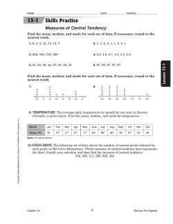


© Copyright 2026