ABC
docz
Explore
Log in
Create new account
Download
Report
business and industrial
business operations
management
project management
CHAPTER 17: MORTGAGE BASICS II: Payments, Yields, & Values
G I OODWILL NDUSTRIES
DRAFT LOAN REQUEST LETTER company on their own letterhead.
Update Car Shopping? July 2014 memcu.com
STUDENT LOAN FUND APPLICATION & AGREEMENT FORM STUDENT DETAILS
Nominations for the American Dialect Society's 2007 Words-of-the-Year Vote
Service, Sincerity and Security Since 1961 INSIDE THIS ISSUE:
1 2014 Start the New Year with a New Car! Ultra-Low Interest Rates!
13 Consumer Mathematics 13.1 The Time Value of Money
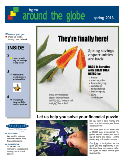
around the globe INSIDE bgcu
All Points Bulletin GREATER PITTSBURGH POLICE FEDERAL CREDIT UNION
Chapter 4 1.
pMT/V5-His A, B, and C user guide Catalog number V4120-20
© Copyright 2026
About abcdocz
DMCA / GDPR
Report