
Document 159766
U.S. Department
of Transportation
http://www.nhtsa.dot.gov
National Highway
Traffic Safety
Administration
____________________________________________________________________________________________
__________
DOT HS 809 662
October 2003
NHTSA Technical Report
Vehicle Weight, Fatality Risk and Crash
Compatibility of Model Year 1991-99
Passenger Cars and Light Trucks
_____________________________________________________________________
________
This document is available to the public from the National Technical Information Service, Springfield, Virginia 22161.
The United States Government does not endorse products or
manufacturers. Trade or manufacturers’ names appear only
because they are considered essential to the object of this report.
Technical Report Documentation Page
1. Report No.
2. Government Accession No.
3. Recipient’s Catalog No.
DOT HS 809 662
4. Title and Subtitle
5. Report Date
Vehicle Weight, Fatality Risk and Crash Compatibility
of Model Year 1991-99 Passenger Cars and Light Trucks
6. Performing Organization Code
7. Author(s)
8. Performing Organization Report No.
October 2003
Charles J. Kahane, Ph.D.
9. Performing Organization Name and Address
10. Work Unit No. (TRAIS)
Evaluation Division; Office of Planning, Evaluation and Budget
National Highway Traffic Safety Administration
Washington, DC 20590
11. Contract or Grant No.
12. Sponsoring Agency Name and Address
13. Type of Report and Period Covered
Department of Transportation
National Highway Traffic Safety Administration
Washington, DC 20590
NHTSA Technical Report
14. Sponsoring Agency Code
15. Supplementary Notes
16. Abstract
Logistic regressions calibrate crash fatality rates per billion miles for model year 1991-99 passenger cars,
pickup trucks, SUVs and vans during calendar years 1995-2000 – by vehicle weight, vehicle type, driver
age and gender, urban/rural, and other vehicle, driver and environmental factors – a cross-sectional
analysis of the fatality rates of existing vehicles. These analyses suggest that, after controlling for driver
age/gender, urban/rural, annual mileage, and other factors:
•
The association between vehicle weight and overall crash fatality rates in the heavier MY 1991-99
LTVs (light trucks and vans) was not significant.
•
In three other groups of MY 1991-99 vehicles – the lighter LTVs, the heavier cars, and especially
the lighter cars – fatality rates increased as weights decreased.
•
MY 1996-99 pickup trucks and SUVs had, on the average, higher fatality rates than MY 1996-99
passenger cars or minivans of comparable weight.
Logistic regression analyses of fatalities per billion miles in two-vehicle collisions show that MY 1991-99
LTVs were more aggressive than MY 1991-99 cars when they struck other vehicles. The analyses show
correlations between occupants’ fatality risk in the struck car and the frontal height-of-force and rigidity
of the striking LTV.
18. Distribution Statement
17. Key Words
mass; safety; car weight; car size; logistic
regression; weight reduction; FARS; statistical
analysis; evaluation; aggressiveness
Document is available to the public through the
National Technical Information Service,
Springfield, Virginia 22161
19. Security Classif. (Of this report)
20. Security Classif. (Of this page)
Unclassified
Unclassified
Form DOT F 1700.7 (8-72)
Reproduction of completed page authorized
21. No. of Pages
325
22. Price
TABLE OF CONTENTS
Acknowledgements....................................................................................................................... v
Executive summary.....................................................................................................................vii
Effects of 100-pound weight reductions on fatality rates ..................................................vii
Fatal-crash and fatality rates by vehicle type, model years 1996-99................................xiii
Car-light truck compatibility...........................................................................................xviii
Limitations of the analyses ............................................................................................... xxi
1.
A new study of vehicle weight and fatality risk and car-light truck compatibility.............. 1
1.1 The need for a new NHTSA study.............................................................................. 1
1.2 Why heavier vehicles have usually had lower fatality rates ....................................... 2
1.3 NHTSA's earlier reports on vehicle weight and fatality risk ...................................... 6
1.4 NHTSA’s car-light truck compatibility research...................................................... 11
1.5 Scope and limitations of this study ........................................................................... 12
2.
Database to study fatalities per million years or billion miles........................................... 15
2.0
2.1
2.2
2.3
2.4
2.5
2.6
3.
Summary ................................................................................................................... 15
Vehicle classification and curb weight ..................................................................... 15
Fatal crash involvements: FARS data reduction....................................................... 19
Vehicle registration years: Polk data reduction ........................................................ 26
Annual mileage and vehicle occupancy: NASS data reduction................................ 26
Induced-exposure crashes: State data reduction ....................................................... 31
Assembling the analysis data files ............................................................................ 36
Vehicle weight and fatality risk in passenger cars............................................................. 41
3.0
3.1
3.2
3.3
3.4
3.5
3.6
3.7
3.8
Summary ................................................................................................................... 41
The calibration data set: 4-door cars, excluding police cars..................................... 41
Visible trends in the data........................................................................................... 43
Screening the control variables; defining the age/gender variables.......................... 63
Regression analyses of fatality risk by car weight.................................................... 75
Summary and discussion of basic regressions .......................................................... 89
“Driver quality” issues and pedestrian fatality rates................................................. 94
Best estimates of the effect of a 100-pound weight reduction.................................. 99
Effect of weight reductions on the number of fatalities.......................................... 104
iii
4.
Vehicle weight and fatality risk in light trucks................................................................ 111
4.0
4.1
4.2
4.3
4.4
4.5
4.6
4.7
4.8
5.
Fatality rates per billion miles in 4-door cars vs. SUVs, pickup trucks and minivans .... 175
5.0
5.1
5.2
5.3
5.4
5.5
5.6
5.7
6.
Summary ................................................................................................................. 111
Visible trends in the data......................................................................................... 111
Screening the control variables............................................................................... 125
Regression analyses of fatality risk by light truck weight ...................................... 128
Sensitivity tests and discussion............................................................................... 145
Best estimates of the effect of a 100-pound weight reduction................................ 153
Effect of weight reductions on the number of fatalities.......................................... 158
The “crossover weight”: crash fatality rates increase for heavier LTVs ................ 163
Comparison with NHTSA’s 1997 report ................................................................ 167
Summary ................................................................................................................. 175
The calibration data set: MY 1996-99 personal-transportation vehicles ................ 175
Unadjusted fatality rates ......................................................................................... 179
Regressions of fatality risk by vehicle type/size group, by crash mode ................. 182
Regressions of overall fatality risk by vehicle type/size group .............................. 194
Fatality rate differences between vehicle types: point estimates ............................ 205
Sources of uncertainty, interval estimates .............................................................. 208
Effect of a different mix of vehicle types on the number of fatalities .................... 220
Car-light truck compatibility: analyses of crash data ...................................................... 225
6.0
6.1
6.2
6.3
6.4
6.5
6.6
6.7
Summary ................................................................................................................. 225
MY 1991-99 LTV aggressiveness in head-on collisions........................................ 225
Frontal rigidity and height-of-force in head-on collisions...................................... 237
Exposure database to study fatality rates in 2-vehicle crashes ............................... 245
MY 1991-99 LTV aggressiveness in 2-vehicle collisions...................................... 249
Frontal rigidity and height-of-force in 2-vehicle collisions.................................... 263
Vehicle weight and crash fatality risk in 2-vehicle crashes.................................... 273
Update of the Mengert-Borener model of car-to-car crash fatality risk ................. 281
References ................................................................................................................................. 283
Appendix A: Curb weights of 1991-99 passenger cars, by model year.................................... 287
Appendix B: Curb weights of 1991-99 light trucks, by model year......................................... 299
iv
ACKNOWLEDGEMENTS
I owe special thanks to Drs. James H. Hedlund, Adrian K. Lund and Donald W. Reinfurt for their
review and comments on a draft of this study and to NHTSA staff reviewers, especially Rory
Austin, Ellen Hertz, Susan Partyka and Stephen Summers.
The effort by Drs. Hedlund, Lund and Reinfurt was not “peer review” of the type used by
journals, but consultation to identify shortcomings in the draft and help NHTSA strengthen this
report. It differed from a peer review in that: (1) We in NHTSA specifically requested and
arranged for these three reviewers. (2) The review process is on record – their comments on the
draft may be viewed in the NHTSA docket for this report. (3) The publication of this report does
not necessarily imply that they “endorsed” it or agreed with its findings. You may read their
comments in the docket to see what they agreed or disagreed with in the draft. We have tried to
address all of the comments in our revised report (but we did not send it back to them for a
second round of review). (4) They went into far more depth and detail than is customary in a
peer review.
v
vi
EXECUTIVE SUMMARY
The National Highway Traffic Safety Administration’s (NHTSA) 1997 report on vehicle weight
and fatality risk estimated the effects of 100-pound reductions in light trucks and vans (LTVs)
and in passenger cars. In the 1997 report, statistical analyses of model year (MY) 1985-93
vehicles in calendar year (CY) 1989-93 crashes found little overall effect for a 100-pound
reduction in LTVs, but an increase of about 300 fatalities per year in cars. However, they also
produced the doubtful findings that vehicle weight reductions do not increase fatality risk in carto-car or LTV-to-LTV crashes and even reduce fatality risk in pedestrian crashes.
NHTSA took a good, hard second look at the subject, identified anomalies in the 1997 report,
and applied different analysis techniques to more recent crash data. This new statistical analysis
of MY 1991-99 vehicles in CY 1995-2000 crashes supersedes NHTSA’s 1997 report.
The new study expands the analyses by separately estimating the effects of 100-pound reductions
in heavy LTVs, light LTVs, heavy cars and light cars. It compares the fatality rates of LTVs and
cars, to quantify differences between vehicle types, given drivers of the same age/gender, etc. In
support of NHTSA’s research on car-LTV compatibility, it analyzes fatality rates in two-vehicle
crashes based on the mass and rigidity of each vehicle and the height mismatch between
vehicles.
Effects of 100-pound weight reductions on fatality rates
In MY 1991-99, and earlier, heavy vehicles had lower fatality rates per billion miles of travel
than lighter vehicles of the same general type. When two vehicles collide, the laws of physics
favor the occupants of the heavier vehicle (momentum conservation). Furthermore, heavy
vehicles were in most cases longer, wider and less fragile than light vehicles. In part because of
this, they usually had greater crashworthiness, structural integrity and directional stability. They
were less rollover-prone and easier for the average driver to control in a panic situation. In other
words, heavier vehicles tended to be more crashworthy and less crash-prone. Some of the
advantages for heavier vehicles are not preordained by the laws of physics, but were nevertheless
characteristic of the MY 1991-99 fleet. Offsetting those advantages, heavier vehicles tended to
be more aggressive in crashes, increasing risk to occupants of the vehicles they collided with.
The statistical analysis uses the Fatality Analysis Reporting System (FARS), R.L. Polk
registration data, State crash data and the National Automotive Sampling System (NASS).
Logistic regressions calibrate crash fatality rates per billion miles for model year 1991-99
vehicles during calendar years 1995-2000 – by vehicle weight, driver age and gender, urban/rural
and other factors discussed and quantified in this report: availability of air bags, ABS, or 4-wheel
drive; vehicle age; annual mileage; speed limit; day/night; wet/dry road; high/low State fatality
rate; and calendar year. “Crash” fatality rates include fatalities to occupants of the case vehicle,
occupants of the other vehicles it collides with, and any pedestrians. The key is to compare
fatality rates of heavy and light vehicles “on a level playing field” by adjusting for differences in
the age and gender of the drivers, the types of roads they travel, and the other factors. In each of
six crash modes that, together, account for over 96 percent of the nation’s crash fatalities, the
vii
analysis calibrates the average increase in the fatality rate for vehicles weighing W-100 pounds
relative to vehicles weighing W pounds, after controlling for driver age/gender and the other
factors – a cross-sectional analysis of the fatality rates of existing vehicles. (Throughout this
study, a vehicle’s “weight” is its “curb weight”: the actual weight of the vehicle with a full tank
of fuel and other fluids needed for travel, but no occupants or cargo.)
Table 1 shows the average fatality increase per 100-pound reduction in LTVs. As stated above,
the “fatality increase per 100-pound reduction” does not mean the effect of literally removing
100 pounds from a specific LTV. It is the average increase in the fatality rates of 1991-99
models weighing W-100 pounds relative to other 1991-99 models weighing W pounds, given
drivers of the same age/gender and equal values on the other factors. The analysis comprises
pickup trucks, SUVs, minivans and full-sized vans. The top half of Table 1 shows the effect in
light trucks weighing 3,870 pounds or more (this was the median weight of LTVs in MY 199199, but the majority of trucks after MY 1995 were heavier). As curb weight decreased by 100
pounds, fatality rates increased by 2.5 to 3 percent in rollovers and fixed-object collisions. Fatal
crashes with pedestrians and heavy trucks were hardly affected. However, in collisions of heavy
LTVs with cars (where 83 percent of the crash fatalities were occupants of the cars) or with
other, usually lighter, LTVs, the 100-pound reduction resulted in a modest net benefit, because it
somewhat reduced risk to the occupants of the other vehicles.
In each crash mode, the percentage effects calibrated for MY 1991-99 vehicles were applied to
the baseline of all CY 1999 crash fatalities in the United States (all model years) to estimate the
annual net fatality change if the mix of LTVs weighing 3,870 pounds or more on the road that
year had averaged 100 pounds lighter – i.e., if the public had purchased fewer of the very heavy
LTVs and more of the make-models weighing not so much in excess of 3,870 pounds. The
increase in rollovers and fixed-object crashes was partly offset by the reduction in LTV-to-car
and LTV-to-LTV fatalities. The point estimate of the net change for all crash modes was an
increase of 71 fatalities, not statistically significant, as evidenced by the interval estimate ranging
from –156 to +241. The interpretation of these interval estimates will be discussed after the
presentation of all the results for LTVs and cars. The point estimate for the percentage change
was a nonsignificant increase of 0.48 percent. The results for the heavier LTVs suggest that
there may have been some weight above 3,870 pounds beyond which overall fatality rates tended
to increase, rather than decrease, as weight increased.
The lower half of Table 1 shows the effect in LTVs weighing less than 3,870 pounds. As curb
weight decreased by 100 pounds, fatality rates increased in every crash mode – although the
observed increases in collisions with pedestrians (1.24 percent) and with cars (1.13 percent) were
small and not statistically significant. In rollovers and collisions with fixed objects, heavy trucks
or other (usually heavier) LTVs, fatality rates increased substantially (3.15 to 6.98 percent) as the
weight of the “case” LTV decreased. The point estimate of the net change for all crash modes in
baseline CY 1999, per 100-pound reduction among the LTVs weighing less than 3,870 pounds,
was an increase of 234 fatalities per year (interval estimate: 59 to 296). The point estimate for
the percentage change was an increase of 2.90 percent.
viii
TABLE 1
FATALITY INCREASE PER 100-POUND WEIGHT REDUCTION, LIGHT TRUCKS
(Baseline = CY 1999 total fatalities, MY 1996-99/CY 1996-2000 fatality distribution)
Annual
Baseline
Crash
Fatalities
Crash Mode
Effect (%) of
100-Pound Reduction
Point
Estimate
Interval
Estimate
Annual Net
Fatality Change
Point
Estimate
Interval
Estimate
LIGHT TRUCKS WEIGHING 3,870 POUNDS OR MORE
Principal rollover
Fixed object
Ped/bike/motorcycle
Heavy truck
Car
Light truck < 3,870
Light truck 3,870 +*
OVERALL
2,183
2,639
2,043
860
5,186
1,010
784
2.56
3.06
.13
.62
- .68
- 1.50
- 3.00
14,705
.48
.81 to
1.41 to
- 1.56 to
- 1.61 to
- 1.79 to
- 3.20 to
- 6.40 to
3.94
4.34
1.45
2.48
.06
- .17
- .34
56
81
3
5
- 35
- 15
- 24
- 1.06 to 1.64
71
18
37
- 32
- 14
- 93
- 32
- 50
to
to
to
to
to
to
to
86
115
30
21
3
-2
-3
- 156 to 241
LIGHT TRUCKS WEIGHING LESS THAN 3,870 POUNDS
Principal rollover
Fixed object
Ped/bike/motorcycle
Heavy truck
Car
Light truck < 3,870*
Light truck 3,870 +
1,319
1,687
1,148
584
2,062
247
1,010
3.15
4.02
1.24
5.91
1.13
6.98
3.49
OVERALL
8,057
2.90
.64 to
1.71 to
- 1.26 to
3.10 to
- .92 to
1.92 to
.96 to
4.30
4.97
2.38
7.36
1.82
9.32
4.66
42
68
14
35
23
17
35
.73 to 3.67
234
__________________
* Assumes both light trucks in the collision were reduced by 100 pounds.
ix
8
29
- 14
18
- 19
5
10
to
to
to
to
to
to
to
57
84
27
46
38
23
47
59 to 296
Table 2 shows the average fatality increase per 100-pound reduction in passenger cars. The
regression analyses are based exclusively on data for 4-door cars, excluding police cars. During
MY 1991-99, only 24 percent of new passenger cars were 2-door models, and fewer than 1
percent of new 4-door cars were police cars. The upper section of Table 2 shows the effect in
cars weighing 2,950 pounds or more (close to the median curb weight of cars throughout MY
1991-99). As curb weight decreased by 100 pounds, fatality rates increased strongly in rollovers
(4.70 percent), decreased non-significantly in pedestrian crashes (0.62 percent reduction), but
increased moderately in all other crash modes (1.59 to 3.18 percent). In absolute terms, though,
the largest increase was in collisions with LTVs (83 per year). The point estimate of the net
change for all crash modes was an increase of 216 fatalities per year (interval estimate: 129 to
303). The point estimate for the percentage change was an increase of 1.98 percent. Those
estimates were somewhat weaker than the effects in light LTVs but much stronger than the
effects in heavy LTVs.
The lower section of Table 2 shows moderate-to-strong effects in every crash mode for cars
weighing less than 2,950 pounds. In rollovers and in collisions with heavy trucks and LTVs,
fatality rates were 5 to 6 percent higher as cars got 100 pounds lighter. Even in pedestrian
collisions, fatality rates rose 3.48 percent. No such increase of pedestrian fatalities was seen in
the heavier cars or either group of LTVs. The point estimate of the net change for all crash
modes was an increase of 597 fatalities per year (interval estimate: 226 to 715), well over double
the increase in the heavier cars or the lighter LTVs. The point estimate for the percentage
change was an increase of 4.39 percent.
The strong increase in pedestrian fatalities for the lightest cars is surprising. At least at first
glance, the weight of the vehicle shouldn’t have had much effect on the fatality risk of
pedestrians. Perhaps, heavier vehicles were simply driven better, even after adjusting for the
drivers’ age/gender, urban/rural and other factors. For example, safety-conscious drivers might
have selected heavier cars because they considered them safer. Heavier cars, more expensive on
the average, might also have attracted higher-income owners with a more health-conscious, less
risk-prone lifestyle. This study, however, found that light and heavy 4-door cars, pickup trucks
and 4-door SUVs of MY 1991-99 all had remarkably similar incidence of high-risk driving
behavior: drinking, speeding, previous crashes, license suspensions, etc. (Two-door cars had
substantially higher-than-average incidence of high-risk driving behavior, but they were not
included in the data used to calibrate the weight-safety relationships.) NHTSA research suggests
that the geometry of small cars might, in fact, have increased the risk of serious injury to
pedestrians (shorter hoods, more head impacts with the windshield frame). Finally, small cars,
because they felt more maneuverable, might even have induced drivers to weave in traffic or take
other risks they would ordinarily have avoided in a larger vehicle.
We do not know how much of the observed effect in pedestrian crashes was due to self-selection
– better drivers picking bigger cars – but we are confident that much of the effect, quite possibly
even all of it was “real.” Thus, the maximum proportion that was self-selection may have been
as low as zero, but it was definitely less than 100 percent. In the absence of evidence supporting
any specific proportion between zero and 100 percent, this report takes the midpoint and assumes
at most half the observed effect in pedestrian crashes was due to self-selection.
x
TABLE 2
FATALITY INCREASE PER 100-POUND WEIGHT REDUCTION, PASSENGER CARS
(Baseline = CY 1999 total fatalities, MY 1996-99/CY 1996-2000 fatality distribution)
Crash Mode
Annual
Baseline
Crash
Fatalities
Effect (%) of
100-Pound Reduction
Point
Estimate
Interval
Estimate
Annual Net
Fatality Change
Point
Estimate
Interval
Estimate
CARS WEIGHING 2,950 POUNDS OR MORE
Principal rollover
Fixed object
Ped/bike/motorcycle
Heavy truck
Car < 2,950
Car 2,950 +*
Light truck
OVERALL
715
2,822
1,349
822
1,342
677
3,157
4.70
1.67
- .62
2.06
1.59
3.18
2.62
2.40 to 7.00
0.63 to 2.71
- 1.83 to .59
.67 to 3.45
.70 to 2.48
1.40 to 4.96
1.74 to 3.50
34
47
- 8
17
21
22
83
17
18
- 25
6
9
9
55
to 50
to 76
to 8
to 28
to 33
to 34
to 110
10,884
1.98
1.19 to 2.78
216
129 to 303
CARS WEIGHING LESS THAN 2,950 POUNDS
Principal rollover
Fixed object
Ped/bike/motorcycle
Heavy truck
Car < 2,950*
Car 2,950 +
Light truck
OVERALL
995
3,357
1,741
1,148
934
1,342
4,091
5.08
3.22
3.48
5.96
4.96
2.48
5.63
.87 to 7.55
.25 to 4.45
.22 to 5.00
2.50 to 7.68
- .72 to 7.16
- .36 to 3.58
2.85 to 6.67
51
108
61
68
46
33
230
9
8
4
29
- 7
- 5
117
13,608
4.39
1.66 to 5.25
597
226 to 715
__________________
* Assumes both cars in the collision were reduced by 100 pounds.
xi
to 75
to 149
to 87
to 88
to 67
to 48
to 273
If so, self-selection also played a role in the other crash modes, not just pedestrian crashes.
Therefore, the interval estimates of this study include not only sampling error but also an
adjustment – up to half of the observed effect in pedestrian crashes – to account for possible
effects due to self-selection.
The interval estimates in Tables 1 and 2 (and also Table 4) are defined as follows: the upper
bound is the point estimate plus 1.96 standard deviations of sampling error (from various known
sources). The lower bound is the point estimate, minus 1.96 standard deviations of sampling
error, minus half the observed pedestrian effect (and, in Table 1, minus an additional allowance
for some uncertainty in the model formulation). The interval estimates are a tool for gauging
uncertainty, but they are not rigorous 95 percent confidence bounds. When the range in the
interval estimate includes zero, the point estimate can be called “not statistically significant.”
When the interval is entirely positive, or entirely negative, it provides some evidence that the
observed effect is “real” – the tighter the interval, the stronger the evidence – but the intervals are
not rigorous confidence bounds, as they would be, for example, in a simple, controlled
experiment.
Table 2, showing a strong increase in fatality risk per 100-pound reduction in cars weighing less
than 2,950 pounds, is based on an analysis including drivers of all ages. When the analysis was
limited to drivers age 60 or older, all the size-safety effects became even more severe, in some
crash modes more than double. That suggests older drivers had serious problems controlling the
lightest cars and/or that the crash environment in light cars in some way amplified older
occupants’ general vulnerability to injury.
The point estimates in Tables 1 and 2 are approximately linear and additive. If, in general,
vehicles weighing W-100 pounds had on the average 1 percent higher fatality rates than vehicles
weighing W, then vehicles weighing W-200 pounds would have had approximately 2 percent
higher rates than vehicles weighing W. The effect of reducing all LTVs by 100 pounds would
have been close to the sum of the effects of reducing LTVs over 3,870 pounds and under 3,870
pounds by 100 pounds each: 71 + 234 = 305.
This study estimates a substantially larger fatality increase per 100-pound weight reduction than
NHTSA’s 1997 report. A review of the 1997 report reveals flaws in the calibration procedure
leading to a systematic underestimate of the size-safety effect in every crash mode, for both
LTVs and cars. This study’s results supersede the 1997 report and, in particular, correct its
findings on car-to-car crashes. Table 2 now shows fatality risk in car-to-car crashes increased as
car weight decreased, consistent with intuition and most of the literature. The lighter cars had
higher crash involvement rates and higher fatality risk, given a crash, for their own occupants.
That more than offset the reduction in fatality risk of occupants in the “other” car.
In summary, Tables 1 and 2 suggest that the association between curb weight and fatality risk in
MY 1991-99 vehicles was weakest – in fact, nonsignificant – in the heavier LTVs. It was
strongest in the lighter cars.
xii
Fatal-crash and fatality rates by vehicle type, model years 1996-99
LTVs of the 1990’s included some models that had high rollover fatality rates per billion miles.
They also included models that, when they collided with other vehicles, the occupant fatality rate
was high in the other vehicle. These LTV models may be characterized as “rollover-prone
and/or aggressive vehicles.” The fatal-crash involvement rates and occupant fatality rates of
different vehicle types were compared on as “level a playing field” as possible, by adjusting for
differences in driver age/gender, annual mileage, vehicle occupancy (where appropriate),
distribution of the mileage by urban/rural, speed limit, and other vehicle, driver and
environmental factors – but not for vehicle weight.
The statistical approach, based on logistic regressions and data similar to the preceding analyses,
was to compare fatal-crash rates per billion vehicle miles for ten groups of model year 1996-99
vehicles during calendar years 1996-2000: four size groups of 4-door cars, three size groups of
4-door SUVs, two sizes of pickup trucks, and minivans. All vehicles were equipped with air
bags. Heavy-duty (200/300-series) pickup trucks and full-sized vans were not included in this
analysis. A single “prorated fatal-crash rate” per billion vehicle miles, comprising all crash
modes, was computed for each vehicle group, after adjustment for driver age/gender, urban/rural,
and other factors. The prorated fatal-crash rates included fatalities to occupants of the case
vehicle, occupants of the other vehicles it collided with, and any pedestrians. Each crash was
weighted by the number of fatalities; however, in order to prevent double-counting, the number
of fatalities in multivehicle crashes was divided by the number of cars/LTVs involved in the
crash (e.g., in a 2-vehicle crash, each vehicle was assigned half the crash fatalities).
Table 3 compares the average curb weights and the overall fatal-crash rates of the ten groups.
Groups that included numerous rollover-prone and/or aggressive vehicles in MY 1996-99 had
greater fatal-crash rates. For example, mid-size 4-door SUVs of model years 1996-99 had an
average fatal-crash rate of 13.68. Similarly, large SUVs and pickup trucks had higher fatal-crash
rates than some groups of cars or minivans. The four vehicle groups with the lowest overall
prorated fatal-crash rates in Table 3 were large cars (7.12), minivans (7.97), mid-size cars (9.46)
and large (100-series) pickup trucks (9.56). Very small 4-door cars had the highest rate (15.73).
However, by 1996-99, these cars only accounted for well under 1 percent of vehicle sales.
xiii
TABLE 3
ADJUSTED FATAL-CRASH INVOLVEMENT RATES
PER BILLION CASE VEHICLE MILES, BY VEHICLE TYPE
(Case vehicles are MY 1996-99 light trucks and 4-door cars with air bags in CY 1996-2000,
adjusted for age/gender, rural/urban, day/night, speed limit, and other factors)
Vehicle Type and Size
Average
Curb
Weight
Prorated* Fatal
Crash Involvements
Per Billion Miles
Very small 4-door cars
Small 4-door cars
Mid-size 4-door cars
Large 4-door cars
2,105
2,469
3,061
3,596
15.73
11.37
9.46
7.12
Compact pickup trucks
Large (100-series) pickup trucks
3,339
4,458
11.74
9.56
Small 4-door SUVs
Mid-size 4-door SUVs
Large 4-door SUVs
3,147
4,022
5,141
10.47
13.68
10.03
Minivans
3,942
7.97
* Each fatal crash involvement by a case vehicle is weighted by: the number of crash fatalities
divided by the number of cars/LTVs involved in the crash.
xiv
Furthermore, 1996-99 SUVs had higher fatality risk for their own occupants than large cars or
minivans. Here, for example, are drivers’ fatality rates per billion vehicle miles (adjusted for
driver age/gender, urban/rural, and other factors):
Driver Fatalities per
Billion Vehicle Miles
Very small 4-door cars
Small 4-door cars
Mid-size 4-door cars
Large 4-door cars
11.56
7.85
5.26
3.30
Compact pickup trucks
Large (100-series) pickup trucks
6.82
4.07
Small 4-door SUVs
Mid-size 4-door SUVs
Large 4-door SUVs
5.68
6.73
3.79
Minivans
2.76
The four vehicle groups with the lowest fatality rates for their own drivers were minivans (2.76),
large cars (3.30), large SUVs (3.79), and large (100-series) pickup trucks (4.07).
Table 3 shows the fatal-crash rate was lower for small 4-door SUVs (10.47) than for mid-size
4-door SUVs (13.68) in MY 1996-99. The drivers’ fatality rate per billion vehicle miles was
likewise lower in small SUVs (5.68) than mid-size SUVs (6.73). This was the only exception to
the customary trend, where larger size groups of the same vehicle type had lower fatal-crash
rates and occupant fatality rates.
A more detailed comparison of the fatality rates of small SUVs, mid-size SUVs and mid-size
cars of MY 1996-99 shows that rollovers and occupants of the “other” vehicle in 2-vehicle
crashes accounted for the higher risk of the SUVs. The small SUVs had much lower rollover
fatality rates than the mid-size SUVs, although still high compared to the cars. Similarly, the
fatality rate for occupants of other vehicles, per billion case-vehicle miles, was substantially
lower for the small-SUV case vehicles than for the mid-size SUVs, but still high compared to the
cars. By contrast, the fatality rates for the vehicles’ own occupants in non-rollover crashes, per
billion occupant miles, were fairly similar for the three types of vehicles, and actually lowest for
the mid-size SUVs:
xv
Fatalities per Billion Miles (Not Prorated)
Small
4-Door
SUVs
Mid-Size
4-Door
SUVs
Mid-Size
4-Door
Cars
Rollovers
Occupants of other vehicles
1.06
3.44
2.71
4.46
.50
2.55
Occupants of case vehicle, in non-rollovers
4.38
3.95
4.63
As stated above, LTVs of the 1990’s included numerous rollover-prone and/or aggressive
vehicles. However, by 1996-99, several new models of small 4-door SUVs with improved
rollover stability had been introduced. For example, one model was measured by NHTSA and
rated substantially more stable than most mid-size or large SUVs of the mid-1990’s. The above
statistics suggest that small 4-door SUVs of 1996-99 may have been the beginning of a new
generation of more stable, less aggressive vehicles with lower fatal-crash rates. This trend
appears to have continued and expanded since 1999, comprising entirely new designs such as
car-based “crossover” SUVs and less sweeping redesigns of existing LTVs. Indeed, rolloverresistance ratings published by NHTSA in 2001 show new models of SUVs in all three size
groups with greater stability than the models they superseded. Also, new technologies such as
“blocker bars” have been introduced on some LTVs to make them less aggressive in collisions
with other vehicles.
Table 3’s adjusted fatal-crash rates for the ten groups of MY 1996-99 vehicles can be applied to
the baseline of all CY 1999 crash fatalities in the United States (all model years) to estimate the
annual change in fatalities if the mix of vehicle types on the road in 1999 had changed – i.e., if
the public had purchased more vehicles of one type and fewer of another. Table 4 estimates the
reduction in fatalities given nine hypothetical scenarios in which the MY 1996-99 vehicle mix
changed to more of one type of car or minivan and fewer of one type of SUV or pickup truck.
For comparison purposes, it also considers one more scenario: a change from very small 4-door
cars to small 4-door cars. It estimates what might have been the annual effect of a “one
percentage point change” in the vehicle mix. For example, during MY 1996-99, mid-size 4-door
SUVs accounted for 8 percent of new-vehicle sales, and large 4-door cars, 12 percent. Table 4
assumes MY 1996-99 vehicles constituted the entire on-road fleet and estimates the effect on
fatalities in baseline CY 1999 if the vehicle mix had instead consisted of 7 rather than 8 percent
mid-size SUVs and 13 rather than 12 percent large cars.
The first nine scenarios in Table 4 all combine a likely reduction in fatalities with a reduction in
vehicle weight. The point estimates of the fatality reductions in Table 4 range from 29 to 200
per year, per percentage point change in the vehicle mix. The reductions for the scenarios
involving changes from mid-size or full-size SUVs to cars or minivans have wholly positive
interval estimates. By comparison, the change from very small cars to small cars is estimated to
reduce fatalities by 156 (with a weight increase). Of course, all these estimates are specifically
for MY 1996-99, a time when numerous pickup trucks and SUVs were rollover-prone or
aggressive.
xvi
TABLE 4
CHANGE IN FATALITIES PER YEAR
GIVEN A ONE-PERCENTAGE POINT CHANGE IN THE ON-ROAD FLEET
FROM MY 1996-99 SUVs AND PICKUPS TO CARS OR MINIVANS
(Baseline = CY 1999 total fatalities, MY 1996-99/CY 1996-2000 fatality distribution)
Fatality Reduction Per Year
Weight
Reduction
Per Vehicle
Point
Estimate
Mid-size 4-dr cars
86
29
– 72 to 64
Mid-size 4-dr SUVs Mid-size 4-dr cars
961
129
79 to 152
Large 4-door cars
426
200
140 to 220
80
174
130 to 201
Large 4-door cars
1,545
101
27 to 133
Minivans
1,199
72
17 to 111
Versus
Small 4-dr SUVs
Minivans
Large 4-dr SUVs
Interval
Estimate
Compact pickups
Mid-size 4-dr cars
278
103
– 57 to 163
Large pickups*
Large 4-dr cars
862
127
– 65 to 194
Minivans
516
82
– 80 to 161
…………………………………………………………………………………………………….
Very small 4-dr cars Small 4-dr cars
– 364
156
– 40 to 231
*Large, standard-duty (100 series) trucks. Excludes heavy-duty 200/300 series pickup trucks.
xvii
Car-light truck compatibility
NHTSA has been researching car-light truck compatibility since 1993. In collisions between
LTVs and cars, approximately 80 percent of the fatalities are occupants of the cars. The
objective is to reduce fatality risk in the car, without increasing risk in the LTV. That may
require increasing crashworthiness of the car, but it might be easier to accomplish by reducing
the aggressiveness of the LTV, or by a judicious combination of both. Of course, MY 1991-99
LTVs usually outweighed cars but, in addition, there were two sources of mismatch between
LTVs and cars that made the LTVs extra “aggressive” when they hit the cars:
•
Structural incompatibility: the LTV’s front was more rigid than any part of the car
•
Geometric incompatibility: the LTV’s front applied its force at a height above the car’s
structures designed to withstand force
The databases and logistic-regression analysis methods used to study vehicle weight and fatality
risk were also suitable for investigating car-LTV compatibility. Fatality rates in 2-vehicle
collisions, per billion miles of each vehicle, were calibrated as a function of the body type and
curb weight of each vehicle (MY 1991-99 in CY 1995-2000), the age/gender of each driver,
urban/rural location, speed limit, and other vehicle, driver and environmental factors. Once
again, the objective was to compare the fatality rates in car-to-car and LTV-to-car collisions on
as “level a playing field” as possible. The first goal was to quantify the extra aggressiveness of
MY 1991-99 LTVs relative to MY 1991-99 cars of the same weight. The analysis focused on
collisions where the struck vehicle was a car, and the striking vehicle was a car, pickup truck,
SUV or minivan. Table 5 shows how much the fatality risk of the driver of the struck car
increased when the striking vehicle was an LTV.
The first row of Table 5 evaluates left-side impacts to the struck car by the front of the striking
vehicle. Left-side impacts are the most dangerous for drivers, because they sit on the left. When
the striking vehicle was a passenger car of weight W, let us say the driver of the struck car had
fatality risk index 100. When the striking vehicle was a pickup truck of weight W, the fatality
risk of the driver of the struck car increased to 177. In other words, it was almost twice as
dangerous, on a per-mile basis, to be hit on the left side by a pickup truck as by a car of the same
weight as that pickup truck. When the striking vehicle was an SUV, the risk index was 235.
Even when the striking vehicle was a minivan, the risk index was 130, higher than when it was a
car. The risk indices for MY 1991-99 pickup trucks, SUVs and minivans were all significantly
higher than 100 in front-to-left impacts.
The second row of Table 5 considers head-on (front-to-front) collisions. Here, LTVs were much
less aggressive. The risk index for the driver of the struck car was significantly higher than 100
only when the striking vehicle was an SUV (132). Impacts by pickup trucks and minivans had
risk indices just slightly, and not significantly, above 100. When they hit cars on the right side or
rear, the aggressiveness of LTVs was higher than in head-on collisions, but not as high as when
they hit the car on the left side. The third row of Table 5 shows that risk indices for pickup
trucks and SUVs were both significantly above 100.
xviii
TABLE 5
AGGRESSIVENESS OF MY 1991-99 LTVs IN IMPACTS WITH MY 1991-99 CARS
AFTER ADJUSTMENT FOR THE STRIKING VEHICLE’S WEIGHT**
(Fatality risk index of the driver of the struck car, by striking vehicle type;
MY 1991-99 vehicles in CY 1995-2000 crashes)
Driver Fatality Risk Index in the Struck Car
by Striking Vehicle Type
Striking Vehicle’s
Front Impacted
the Struck Car on the
Car
Pickup
SUV
Minivan
Left side
100
177*
235*
130*
Front (head-on collision)
100
114
132*
104
Right side or rear
100
139*
162*
125
Anywhere
100
139*
171*
116*
*Significantly greater than 100.
**For example, in a front-to-left impact, if the risk for the driver of the struck car was 100 when
the striking vehicle was a 3,500 pound car, the risk increased to 177 when the striking vehicle
was a 3,500 pound pickup truck.
xix
Combining all of the preceding crash modes, the last row of Table 5 shows that, overall, every
type of MY 1991-99 LTV was significantly more aggressive than a passenger car. All of these
indices apply specifically to MY 1991-99 vehicles and could change for more recent LTVs as
new technologies or designs are introduced to reduce aggressiveness in collisions.
The second analysis goal was to test for association between the aggressiveness of model year
1991-99 LTVs in crashes and physical parameters describing the structural rigidity and geometry
of the trucks. Two parameters were readily available, because NHTSA measures them during its
frontal crash tests in the New Car Assessment Program (NCAP). They are:
Frontal rigidity:
The average slope of the force-deflection profile maintained for at least 150
millimeters during the vehicle’s initial crush in an NCAP frontal impact with
the barrier.
Height-of-force: The average height-of-force measured by load cells set at various height levels
in the NCAP barrier. It is the weighted average of the effective height of the
applied force on the barrier face over the duration of the impact.
Association was tested by limiting the preceding logistic-regression analyses to crashes where
the striking vehicle was an LTV (and the struck vehicle was a car), and adding the two
parameters to the regression. In front-to-left impacts, there was a statistically significant
association between the driver’s fatality risk in the struck car and the difference in the heights-offorce of the striking and struck vehicles: the greater the height mismatch between the LTV and
the car, the greater the fatality risk of the driver of the car. In head-on collisions, the LTV’s
frontal rigidity was significantly associated with the car driver’s fatality risk: the more rigid the
LTV, the greater was the fatality risk of the car driver.
The analyses accept as a given that model year 1991-99 LTVs were, on the average, more
aggressive than cars. These somewhat exploratory findings suggest that the LTVs with the
tallest and most rigid frontal structures were even more aggressive than the other LTVs.
These analyses of car-LTV compatibility are intended to supplement and corroborate, not
supersede NHTSA’s previous work on that subject. This study’s approach, based on fatality
rates per billion miles, controlling for each vehicle’s weight, each driver’s age and gender,
urban/rural, and other factors, helps compare fatality rates in car-car and car-LTV collisions “on
a level playing field.” On the other hand, the per-mile approach does not necessarily separate
crash-proneness from crashworthiness effects (a disadvantage here, although it was a plus in the
size-safety analyses). It is best to look at these results in combination with NHTSA’s previous
findings on car-LTV compatibility. In addition, the statistical findings that show an association
of these two parameters with extra aggressiveness of LTVs do not, by themselves, guarantee that
these two parameters “caused” the aggressiveness, or that they are the parameters that best
explain or measure aggressiveness. Crash testing with existing and, eventually, modified
vehicles is another essential step in learning what makes LTVs aggressive.
xx
Limitations of the analyses
This study is a cross-sectional analysis of the crash fatality rates per billion miles of real MY
1991-99 vehicles in CY 1995-2000: light, mid-size and heavy passenger cars, pickup trucks,
SUVs and vans. Statistical tools calibrated the relationships between vehicle weight and fatality
rates – the average increase for vehicles weighing W-100 pounds relative to vehicles weighing
W pounds – and the differences between cars and LTVs, after controlling for driver age/gender,
urban/rural, and other vehicle, driver and environmental factors. The results specifically
describe the performance of MY 1991-99 vehicles; the impact of new designs or technologies in
more recent vehicles will be revealed as they now accumulate on-the-road experience.
The analysis is not a “controlled experiment.” People are largely free to pick whatever car or
LTV they wish. Owner characteristics and vehicle use patterns can and do vary by vehicle
weight and type. This study adjusts for differences in age/gender, urban/rural driving, and other
factors, and tries to gauge uncertainty due to less tangible variations in “how well people drive.”
But, ultimately, we can never be sure that a 30-year-old male operating a large LTV on an urban
road at 2:00 p.m. in a Western State drives the same way as a 30-year-old male operating a
smaller LTV/light car/heavy car at a similar roadway, time and location. The interval estimates
in this study try to depict likely ranges of uncertainty in the principal findings, but rigorous “95
percent confidence bounds” do not apply here, as they would, for example, in a simple,
controlled experiment.
xxi
xxii
CHAPTER 1
A NEW STUDY OF VEHICLE WEIGHT AND FATALITY RISK
AND CAR-LIGHT TRUCK COMPATIBILITY
1.1
The need for a new NHTSA study
In 1997, the National Highway Traffic Safety Administration (NHTSA) issued seven reports that
addressed vehicle weight and safety by statistically analyzing relationships between existing
vehicles’ curb weights and their fatality and injury rates in crashes.1 One of the reports, a study
of vehicle weight and fatality risk, was NHTSA’s first attempt to estimate the effect of a 100pound reduction in each of the important crash modes, and to do this separately for light trucks
and passenger cars.2 Calibrated from model year (MY) 1985-93 vehicles in calendar year (CY)
1989-93 crashes, the analyses found little overall effect for a 100-pound reduction in light trucks
and vans (LTVs), because increased fatalities of truck occupants were offset by a reduction of
fatalities in the vehicles that collided with the trucks, whereas a 100-pound reduction in cars was
associated with an increase of about 300 fatalities per year.
Unfortunately, the mere fact that the 1997 report addressed all crash modes did not necessarily
make its estimates correct. The 1997 report claimed that fatalities in car-to-car and LTV-to-LTV
crashes decreased as both cars or both LTVs were reduced in weight. That disagrees with
research and empirical data consistently showing that, at least in the past, heavy vehicles tended
to be more crashworthy and less crash-prone than light vehicles. The report’s conclusion that
vehicle weight reductions saved lives in pedestrian crashes is also questionable.
The most important reason for a new study is to take a good, hard second look at the methods of
the 1997 report and to revise or supersede them with techniques that more accurately fit the data.
Another reason for a new study is that the vehicle, crash and driver environment has changed in
six years. Since MY 1985-93 and CY 1989-93, LTVs have become more numerous and heavier;
belt use increased; there are more air bags and older drivers. New models were introduced and
old ones phased out.
1
Kahane, C.J., Relationships between Vehicle Size and Fatality Risk in Model Year 1985-93 Passenger Cars and
Light Trucks, NHTSA Technical Report No. DOT HS 808 570, Washington, 1997; Partyka, S.C., Effect of Vehicle
Weight on Crash-Level Driver Injury Rates, NHTSA Technical Report No. DOT HS 808 571, Washington, 1996;
Partyka, S.C., Passenger Vehicle Weight and Driver Injury Severity, NHTSA Technical Report No. DOT HS 808
572, Washington, 1995; Hertz, E., The Effect of Decreases in Vehicle Weight on Injury Crash Rates, NHTSA
Technical Report No. DOT HS 808 575, Washington, 1997; Partyka, S.C., Patterns of Driver Age, Sex and Belt Use
by Car Weight, NHTSA Technical Report No. DOT HS 808 573, Washington, 1995; Partyka, S.C., Impacts with
Yielding Fixed Objects by Vehicle Weight, NHTSA Technical Report No. DOT HS 808 574, Washington, 1995;
Relationships of Vehicle Weight to Fatality and Injury Risk in Model Year 1985-93 Passenger Cars and Light
Trucks, NHTSA Summary Report No. DOT HS 808 569, 1997.
2
Kahane (1997), op. cit.
1
The third motivation is to expand the analyses. The 1997 report estimated two numbers: the
effect of a 100-pound reduction in LTVs of any weight, and in passenger cars. The new study
separately estimates the effects of 100-pound reductions in heavy LTVs, light LTVs, heavy cars
and light cars. It compares the fatality rates of LTVs and cars, to quantify the differences in the
rates between vehicle types, given drivers of the same age/gender, etc. In support of NHTSA’s
ongoing research on car-LTV compatibility3, this study analyzes fatality rates in two-vehicle
crashes based on the mass and rigidity of each vehicle and the height mismatch between the
vehicles.
This statistical analysis of CY 1995-2000 crash data involving MY 1991-99 vehicles supersedes
NHTSA’s 1997 report on vehicle size and fatality risk.
1.2
Why heavier vehicles have usually had lower fatality rates
One safety factor, momentum conservation, is a direct consequence of a vehicle’s mass. Other
parameters, such as a vehicle’s length and width are naturally and historically (i.e., during 196899), but not inevitably proportional to its mass. Most of those parameters favor the heavier
vehicle, making it physically, intrinsically safer than the light vehicle.
Some human factors of drivers are historically, but not intrinsically confounded with vehicle
mass. For example, young drivers historically have driven smaller cars4, but at least in theory,
they might at some future time prefer large cars. These factors could give heavy vehicles lower
fatality rates, but don’t make them intrinsically safer. The analysis should, as much as possible,
remove these factors and compare the fatality rates of heavy and light vehicles on a level playing
field, leaving only the physical factors that make heavy vehicles safer. Finally, there are inbetween factors where it is not so clear if the relationship with mass is intrinsic or coincidental.
Momentum conservation: When a heavy and a light vehicle collide, the heavy vehicle keeps
moving forward; its occupants experience a small velocity change. The light vehicle gets pushed
backward; its occupants experience a higher velocity change. These are consequences of the
laws of physics; nothing can be done to equalize the velocity changes. For example, in a headon collision, a 1 percent weight advantage corresponds to more than a 5 percent reduction in the
driver's fatality risk, relative to the driver of the other vehicle.5
What benefits an individual – being in the heavier of the two vehicles – however, does not
necessarily benefit society as a whole. Based on momentum considerations alone, the risk
reduction in Vehicle 1 as it becomes heavier is cancelled by a risk increase in Vehicle 2. If
momentum conservation were the only factor making heavier vehicles safer (it isn’t), overall
fatalities in multivehicle crashes would neither increase nor decrease if the entire vehicle fleet
were reduced in mass.
3
Hollowell, W.T., Summers, S.M., and Prasad, A., NHTSA’s Research Program for Vehicle Aggressivity and Fleet
Compatibility, UK IMechE Vehicle Safety 2002 Conference, London, May 2002.
4
For example, the database generated for this study suggests 34 percent of drivers of 4-door cars weighing less than
3,000 pounds are younger than 30, but only 15 percent of drivers of cars weighing over 3,000 pounds.
5
See Section 6.1 of this report.
2
Momentum also enables a heavy vehicle to knock down, displace or brush aside medium-sized
fixed objects that would have brought a lighter vehicle to an abrupt stop.
Crashworthiness: Heavier vehicles have historically done a better job cushioning their occupants
in crashes. Their longer hoods and extra space in the occupant compartment provide an
opportunity for a more gradual deceleration of the vehicle, and of the occupant within the
vehicle. In the New Car Assessment Program, crash test results have been consistently better for
large cars, given the same 35 mph barrier impact.6 While it is conceivable that light vehicles
could be built with similarly long hoods and mild deceleration pulses, it would probably require
major changes in materials and design and/or taking weight out of their engines, accessories, etc.
Structural integrity: Heavier vehicles have historically provided better protection against
intrusion by fixed objects, heavy trucks, etc. Doors, frames, pillars, roof rails, etc. are
thicker and stronger. Since the occupant compartment is larger, these structures also
have more room to deform.7
Rigidity/sill height/aggressiveness: A rigid structure can be helpful in many impacts with fixed
objects. High, strong side sills are important protection if the vehicle is struck in the side. But
high, rigid structure increases the risk to the occupants of other vehicles (aggressiveness), and
rigidity can also make the vehicle’s deceleration more abrupt in some impacts. The database
created in Section 6.2 of this report shows some correlation of rigidity and height-of-force with
curb weight in current vehicles, but a much stronger association these parameters with vehicle
type (some of the MY 1991-99 pickup trucks and SUVs were higher and more rigid than cars or
minivans of the same mass).
Mass mismatch: There is widespread belief that a collision between vehicles of similar mass is
safer than a collision of badly mismatched vehicles. If so, making the heaviest vehicles lighter,
and the lightest heavier, could reduce fatalities in crashes between passenger vehicles.
(However, analyses in Section 6.6 of this report do not show significantly higher fatality rates
per unit of exposure in crashes of 2,000 with 4,000 pound cars than in crashes of two 3,000
pound cars.)
Directional stability/ease of control: The preceding factors affect fatality risk, given that a crash
has occurred. There are also physical factors that tend to make heavier vehicles less crash-prone.
Heaver vehicles, with their typically longer wheelbases, are less prone to skid or spin out of
control in response to braking or steering input, or on an uneven road surface. They are more
likely to stay on the road.8
6
Effect of Car Size on Fatality and Injury Risk, NHTSA, Washington, 1991.
For example, Kahane, C.J., Evaluation of FMVSS 214 Side Impact Protection Dynamic Performance Requirement,
Phase 1, NHTSA Technical Report No. DOT HS 809 004, Washington, 1999, p. 64 shows a steady improvement of
side structure integrity as curb weight increases.
8
Malliaris, A.C., Nicholson, R.M., Hedlund, J.H. and Scheiner, S.R., Problems in Crash Avoidance and in Crash
Avoidance Research, Paper No. 830560, Society of Automotive Engineers, Warrendale, PA, 1983.
7
3
In theory, a sober, alert, expert driver might find a light vehicle more responsive, easier to brake
and steer away from trouble. Unfortunately, many drivers in fatal crashes are impaired,
unskilled, distracted, or at the very least caught off-guard in a panic situation. The quicker
response of light vehicles may give the average driver yet more opportunity to blunder.
Rollover stability: Heavier vehicles, historically, have almost always been wider than light
vehicles of the same class. As a result, they have a higher static stability factor9 and are
substantially less prone to rollover. While it is conceivable that light vehicles could be built just
as wide as heavy vehicles, it would presumably require new designs, materials and/or cutting
weight out of existing structures, accessories, etc.
Availability of safety equipment: During the 1990’s, air bags were often installed a year or two
earlier in the heavier vehicles (easier to install, possibly more consumer demand). Antilock
Brake Systems (ABS) were installed earlier on the larger, more luxurious vehicles and are still
infrequent on small, inexpensive cars.10 Analyses should be able to control for those differences.
The above are physical factors that have historically or intrinsically influenced the fatality rates
in small vs. large vehicles. Here are some human factors of drivers that are confounded with
vehicle weight:
Driver age and gender: This report will present data showing that, historically, lighter vehicles
have somewhat younger drivers; heavier vehicles, especially heavy cars, older drivers. Small 4door cars are especially popular with female drivers. Large cars, LTVs generally, but pickup
trucks especially, are popular with male drivers.
Young and old drivers have far more fatal crashes per million years, or per billion miles than
drivers in the 30-50 age bracket (see Figure 3-15). Up to age 60, males have substantially
higher fatal crash rates than females. Young drivers’ inexperience and aggressiveness, older
drivers’ vision and vehicle-control problems, and male drivers’ aggressiveness/impairment all
contribute to high crash rates. The vulnerability of older occupants to injury further increases
their fatality rates.
Thus, the higher incidence of young drivers inflates the fatality rates of lighter vehicles, but the
higher incidence of female drivers (especially in small 4-door cars) reduces the rates. The
popularity of large cars with older drivers, and LTVs (especially pickup trucks) with males
inflates their fatality rates. It is imperative that the analyses control or adjust fatality rates to
compensate for differences in driver age and gender.
9
Half the track width, divided by the center-of-gravity height.
ABS is effective in reducing certain types of crashes, but may be associated with increases of other types of
crashes at certain times; see Kahane, C.J., Preliminary Evaluation of the Effectiveness of Antilock Brake Systems for
Passenger Cars, NHTSA Technical Report No. DOT HS 808 206, Washington, 1994.
10
4
Urban/rural: Fatality rates per billion miles are higher in rural areas.11 Pickup trucks are
especially common in rural areas (inflating fatality rates), while small cars are more
characteristically urban (deflating the rates).
The preceding human and environmental factors are readily measurable and can be controlled in
the analyses. However, there is another set of somewhat interrelated human factors, not easily
quantified, somehow related with vehicle weight and fatality risk. Briefly stated, heavier
vehicles may be driven better for a variety of reasons that are not clearly understood. These
factors are discussed in Sections 3.6 and 5.6 of this study, and may include:
Vehicle reputation/driver self-selection: Safety-conscious drivers might pick heavier vehicles
because they consider them safer. Also, vehicle brands and body-styles with an excellent
reputation for safety tend to attract safety-conscious drivers and, primarily because of this, have
exceptionally low fatality rates.12 These are often, but not necessarily, heavier vehicles.
Conversely, sporty and high-performance vehicles, especially 2-door cars, attract risk-prone
drivers and have high fatality rates. That could create a “self-fulfilling prophecy,” partially
explaining the lower fatality rates of heavier vehicles.
However, the analyses in Sections 3.6 and 5.6 will show that light and heavy 4-door cars, pickup
trucks and SUVs all have remarkably similar incidence of imprudent driving behavior: drinking,
speeding, previous crashes, license suspensions, etc. Only 2-door cars have substantially higherthan-average incidence of imprudent driving behavior, and only minivans are lower than
average. In this study, 2-door cars will never be included in data used to calibrate the
relationships of weight and fatality risk in passenger cars.
Driver income/vehicle price: Heavier cars are usually, but not always more expensive than light
cars. Their owners are likely to have higher incomes, on the average. Higher income [and
education] has been associated with a more health-conscious, less risk-prone lifestyle. That may
include driving more prudently. (See discussion in Section 3.6.)
Smaller vehicles weave in traffic: It is possible that drivers of small vehicles are more likely to
weave around in traffic, change lanes, dart ahead of others or even take corners and curves faster.
If so, what is the cause and what is the effect? Is it merely less prudent drivers self-selecting
smaller vehicles, as suggested above? Or do the smaller vehicles themselves, because they feel
more maneuverable, induce drivers to take risks they would ordinarily avoid in a larger vehicle?
The principal estimates of this study include an allowance (in the interval estimates) that some of
the observed relationship between vehicle size and fatality rates could be due to better drivers
self-selecting larger vehicles, rather than the intrinsic characteristics of the vehicles.
But these driver effects, while they should not be ignored, are probably of limited importance.
The relationship of car weight to fatality risk is calibrated from data on 4-door cars (excluding
police cars). During the late 1990’s, small 4-door cars were especially popular with 30-50 year
11
Accident Facts, 1993 Edition, National Safety Council, Itasca, IL, 1993, p. 64.
Kahane, C.J., Correlation of NCAP Performance with Fatality Risk in Actual Head-On Collisions, NHTSA
Technical Report No. DOT HS 808 061, Washington, 1994, pp. 3-7.
12
5
old women. Although there are, of course, individual variations within that group, they are,
overall, the safest and most prudent drivers on the road. It is more correct to say that small 4door cars had high fatality rates despite, rather than because of the people who drove them.
1.3
NHTSA's earlier reports on vehicle weight and fatality risk
NHTSA’s 1997 report estimated the percentage increase (or decrease) in crash fatalities
(including occupants of other vehicles, and pedestrians) per 100-pound weight reduction, in each
of the important crash modes, separately for passenger cars and LTVs:13
NHTSA 1997
Crash Mode
Fatality Increase (%) Per 100 Pound Reduction
Passenger Cars
Light Trucks
Principal rollover
Hit object
Hit ped/bike/motorcycle
Hit heavy truck
Hit passenger car
Hit light truck
+ 4.58
+ 1.12
– .46
+ 1.40
– .62 *
+ 2.63
+ .81 *
+ 1.44
– 2.03
+ 2.63
– 1.39
– .54 *
OVERALL
+ 1.13
–
.26 *
* Not statistically significant
The analysis associated a 100-pound reduction in cars with a significant increase of 302 crash
fatalities per year, and a 100-pound reduction in LTVs with a reduction of 40 crash fatalities per
year (not statistically significant).
The analysis was a regression of fatality rates per million vehicle registration years, based on
Fatality Analysis Reporting System (FARS) and Polk registration data for MY 1985-93 vehicles
in CY 1989-93 crashes. However, State crash data were used in a quite indirect way to adjust
these rates for differences in driver age and gender. Section 4.8 of this study extensively
critiques the methods of the 1997 report. In brief, the 1997 report concluded that lighter vehicles
are safer than indicated by their raw fatality rates per million years, based on the following
implicit (and essentially “hidden”) inferences from the adjustment procedure:
•
13
Heavy cars and LTVs are driven fewer miles per year than mid-size vehicles, because
they have older drivers, and older people drive fewer miles per year.
Kahane (1997), op. cit., pp. vi-vii.
6
•
Light cars and LTVs are driven more miles per year than mid-sized vehicles, because
they have younger drivers, and young people drive more miles per year.
•
Therefore, the simple per-year fatality rates understate their per-mile rates of heavy
vehicles, but overstate the rates of lighter vehicles. After the adjustment, the safety
advantage of heavier vehicles shrinks for cars and vanishes for LTVs
All of these statements are false, except that older people drive fewer miles per year. In fact,
odometer readings from the National Automotive Sampling System (NASS) show that light,
mid-size and heavy cars are driven almost equal numbers of miles per year, whereas heavy LTVs
are driven substantially more miles per year than light LTVs of the same type. It is also untrue
that young people drive more miles per year than 25-50 year old adults. (See Section 2.4 of this
report.) As a result, the 1997 report underestimated the fatality increases associated with weight
reductions – in every crash mode, for both cars and LTVs. An additional source of bias was the
inclusion of 2-door cars and police cars in the calibration of the weight-safety effect in passenger
cars. High-performance 2-door cars weighing about 3,000 pounds had very high fatality rates in
some crash modes and police cars weighing about 3,700 pounds had high rates in other modes,
enough to throw the calibration off the real trend lines of fatality rates by vehicle weight.
In most crash modes the true effect was large enough that, even with these biases, the 1997
report still estimated a fatality increase. However in car-to-car, LTV-to-LTV and pedestrian
crashes, where the true effect was smaller, the 1997 report associated fatality reductions with
weight reductions. As stated above, those results now seem counterintuitive.
How did this problem escape earlier detection at NHTSA? As the critique (Section 4.8 of this
study) explains, the implicit assumptions about annual mileage are quite well hidden and are
only revealed by scrutiny of some regression coefficients in the 1997 report. But why didn’t
NHTSA staff look at the car-to-car results and say, “This can’t be right, let’s keep reviewing the
model until we find the problem”? In fact, NHTSA was already conditioned to believe that the
effect of weight reductions on car-to-car crash fatalities might be negligible, because its pre-1997
analyses, due to biases or data flaws of their own, produced similar results.
In 1989-91, NHTSA staff analyzed relationships of passenger-car weight and fatality risk in
three crash modes: rollovers, fixed-object and car-to-car. All three results are indeed very close
to the 1997 report:
7
NHTSA 1991
Crash Mode
Principal rollover
Hit object
Hit ped/bike/motorcycle
Hit heavy truck
Hit passenger car
Hit light truck
Fatality Increase (%) Per 100 Pound Reduction
Passenger Cars
+ 3.5
+ .9
not analyzed
not analyzed
Not statistically significant
not analyzed
Klein, Hertz and Borener performed the analyses of fixed-object and car-to-car crashes.14
Logistic regressions of 1984-87 Texas and 1984-88 Maryland crash data calibrated drivers'
fatality risk per 100 towaway crash involvements, as a function of vehicle weight, driver age and
gender, crash mode, and other variables (in car-to-car crashes: the case car driver’s fatality risk
per 100 involvements as a function of both vehicles’ weights, both drivers’ ages, and other
factors). The model finds no significant change in drivers’ fatality risk when each car in a 2-car
collision is reduced by 100 pounds, but all other variables stay the same. The fatality rate in
fixed-object collisions increases by a modest but significant 0.9 percent for each 100-pound
weight reduction. (The 1997 report also found no significant effect in 2-car crashes and a 1.12
percent increase in collisions with fixed objects.)
The analysis method based on fatalities per 100 reported towaway crashes, customary at that
time and widely used even today, creates a twofold bias in favor of smaller cars and
underestimates the fatality increase per 100-pound reduction:
•
By considering the probability of fatality given that a crash has already occurred, the
method only measures differences in crashworthiness. It ignores the superior directional
stability/ease of control of larger cars, that enables them to stay out of crashes entirely
(especially run-off-road/fixed object crashes).
•
The measure of exposure (denominator of the fatality rate) – reported towaway crash
involvements – is itself confounded with vehicle weight. Heavier cars and LTVs have
substantially fewer reported towaway crashes per million miles than small cars. As stated
above, they have fewer crashes. Because they are more rugged, even if they have a crash,
it is less likely to require towaway. An impact that just dents a big station wagon might
disable a small, light car. Finally, even if there is a towaway, it is less likely that a police
report will be filed – if nobody is injured and the damage is not especially severe (e.g.,
when the cars are no longer brand-new).
14
Klein, T.M., Hertz, E. and Borener, S., A Collection of Recent Analyses of Vehicle Weight and Safety, NHTSA
Technical Report No. DOT HS 807 677, Washington, 1991; summarized in Effect of Car Size on Fatality and Injury
Risk, NHTSA, Washington, 1991.
8
Kahane analyzed fatal rollover crashes of MY 1970-82 cars in CY 1975-86 FARS data.15 The
ratios of fatalities in most-harmful-event rollovers to fatalities in frontal impacts with fixed
objects were computed for cars of various size groups. The analysis did not control for driver
age or gender. The ratio increased by 3.5 percent per 100-pound weight reduction. This report,
too, underestimated the size-safety effect because it considered the frontal impacts a control
group with equal fatality risk at all car weights. In reality, fatality risk in fixed-object collisions
also increases as car weight is reduced. A more correct conclusion of the report would have
been: rollover fatalities increase 3.5 percent faster than frontal fixed-object fatalities, per 100pound weight reduction.
The results of this report, based on MY 1970-82 cars, are remarkably similar to the current study,
based on MY 1991-99 cars. Historically, lighter cars have more rollover fatalities because they
are also narrower and shorter cars. Of course, there is a natural correlation of mass, width and
length, but at least in theory it should be possible to change one and not the others (e.g., by using
different materials). The two studies show how little the relationships of mass, width, length and
rollover risk have changed in the last 30 years.
NHTSA also sponsored Mengert and Borener's 1989 analysis of fatal crashes, based on MY
1978-87 cars in CY 1978-87 FARS and Polk data.16 Separate analyses address four crash modes
which, together, comprise essentially all fatal crashes involving cars. The measure of risk, crash
fatalities per million car years (including pedestrians and occupants of other vehicles in the
crash) is similar to this study and NHTSA’s 1997 report. It accounts for crash-avoidance as well
as crashworthiness effects. However, their analysis did not adjust for driver age, gender, or any
other factor that is confounded with vehicle mass and correlated with fatality risk.
Cars were subdivided into six weight groups. In the three crash modes involving a single
passenger car, a relative fatality risk was obtained for each of the six weight groups: the
proportion of the fatalities F i in weight group i was divided by that weight group's proportion of
car registrations R i. For example, if cars in the lightest weight group account for F 1 = 15
percent of the single-vehicle crash fatalities and R 1 = 10 percent of car registrations, the relative
risk is 1.5. In the car-to-car crash mode, the relative risk was obtained for each of the 36 pairs of
weight groups: the proportion of car-to-car fatalities F i j involving a car of weight group i and a
car of group j was divided by R i R j . For example, if collisions between cars of the lightest
weight group and the heaviest weight group account for F 1 6 = 1 percent of car-to-car fatalities, R
1 = 10 percent and R 6 = 5 percent of car registrations, then the relative risk is 2.0. With these
measures of relative risk, Mengert and Borener could estimate the net effect on total fatalities for
any hypothetical future change in the distribution of car registrations among the six weight
groups.
15
Kahane, C.J., “Effect of Car Size on the Frequency and Severity of Rollover Crashes,” Proceedings of the
Thirteenth International Technical Conference on Experimental Safety Vehicles, NHTSA, Washington, 1991, Paper
No. 91-S6-W-12.
16
Mengert, P., Estimating Relative Safety of Hypothetical Weight Distribution for the National Passenger Car
Population, 1989 SAE Government/Industry Meeting, Washington, May 3, 1989.
9
If all passenger cars were to be reduced in weight by 100 pounds, while vehicles other than
passenger cars remain unchanged, the Mengert-Borener model predicted the following effects on
crash fatalities:
Mengert-Borener 1989
Fatality Increase (%) Per 100 Pound Reduction
Crash Mode
Passenger Cars
Rollover or hit object
Hit pedestrian/bike
Hit LTV/heavy truck/motorcycle
Hit passenger car
+ 2.0
– 2.4
+ 1.0
– .8
OVERALL
+ .5
These results, too, are consistent with the small overall size-safety effect in NHTSA’s 1997
report, and in particular show a reduction in car-to-car and car-to-pedestrian crash fatalities as
car weight is reduced. The detrimental effects of weight reduction were confined to singlevehicle crashes and collisions with LTVs and heavy trucks.
However, when the analyses were limited to later calendar years of FARS data, all the results
shifted substantially in favor of larger cars: the effect of a 100-pound reduction became 1 to 2
percentage points stronger (or less negative) in each crash mode. It is unknown why the full
model showed such small size-safety effects, or why the results shifted in later calendar years of
FARS. Possible issues include:
•
The absence of any control for driver age/gender, urban/rural, etc.
•
The inclusion of 2-door cars in the analysis. High-performance cars weighing about
3,000 pounds might have fatality rates high enough to influence overall results.
•
The use of only six weight classes might have created unexpected discontinuities.
Section 6.7 of this report updates the Mengert-Borener analysis of car-to-car crashes, applying
their model to CY 1995-2000 FARS data on MY 1991-99 cars – but limited to 4-door cars and
using ten rather than six weight classes. The effect of a 100-pound reduction is an intuitively
much more reasonable 2.74 percent fatality increase, not the 0.8 percent decrease seen by
Mengert and Borener. Unfortunately, this new result was not available in 1995-97. Thus, the
Mengert-Borener study and NHTSA’s 1989-91 analyses may both have conditioned NHTSA
staff not to be alarmed when their 1997 analyses did not show a significant increase in car-to-car
crash fatalities as car weight decreased.
10
Of course, NHTSA is not the only organization studying relationships between vehicle size and
fatality risk. For example, as early as 1982-84, Evans analyzed a group of car crashes including
rollovers, fixed-object impacts and collisions with heavy trucks and LTVs.17 He calibrated that
fatality risk increased by 2.6 to 4.8 percent per 100-pound reduction of car weight. The range is
quite consistent with the results of this study, nearly 20 years later. The National Research
Council's 1992 analysis of fuel economy issues extensively reviewed the size-safety literature.18
1.4
NHTSA’s car-light truck compatibility research
The agency has been researching fleet compatibility since 1993.19 The long-term goal is to
develop safety standards that will reduce crash fatalities and injuries for the entire vehicle fleet,
while also providing a high degree of safety in each type of vehicle. In collisions between two
different types of vehicles, say a large LTV and a small car, the objective is to reduce fatality risk
in the car, without increasing risk in the LTV. That may require increasing crashworthiness of
the car, but it might be better accomplished by reducing the aggressiveness of the LTV, or by a
judicious combination of both. The research has identified three main sources of mismatch
between vehicles:
•
•
•
Mass incompatibility (one vehicle is much heavier than the other)
Structural incompatibility (one vehicle is much more rigid than the other)
Geometric incompatibility (one vehicle applies force at a height above the other
vehicle’s structures designed to withstand force)
Mass is easily measured placing a vehicle on scales. NHTSA’s research staff has identified ways
to measure vehicles’ rigidity and height-of-force using data collected during NHTSA’s crash
tests.
NHTSA has also sponsored extensive statistical analyses, based on crash data, of the relative
aggressiveness and compatibility of various vehicles, and the relationships of vehicles’ rigidity
and height-of-force to their aggressiveness in actual crashes.20 Unlike the size-safety analyses,
where this study’s goal is to supersede all estimates in NHTSA’s 1997 report, this study’s
17
Evans, L., Car Mass and the Likelihood of Occupant Fatality, Paper No. 820807, Society of Automotive
Engineers, Warrendale, PA, 1982; Evans, L., “Driver Fatalities versus Car Mass Using a New Exposure Approach,”
Accident Analysis and Prevention, Vol. 16, 1984, pp. 19-36; see also Crandall, R.W., and Graham, J.D., “The Effect
of Fuel Economy Standards on Automobile Safety,” Journal of Law and Economics, 1989.
18
Automotive Fuel Economy: How Far Should We Go?, National Academy Press, Washington, 1992, pp. 47-68.
19
Gabler, H.C. and Hollowell, W.T., “NHTSA’s Vehicle Aggressivity and Compatibility Research Program,”
Proceedings of the Sixteenth International Technical Conference on the Enhanced Safety of Vehicles, NHTSA,
Washington, 1996, Paper No. 98-S3-O-12; Gabler, H.C. and Hollowell, W.T., The Aggressivity of Light Trucks and
Vans in Traffic Crashes, Paper No. 980908, Society of Automotive Engineers, Warrendale, PA, 1998; Gabler, H.C.
and Hollowell, W.T., “The Crash Compatibility of Cars and Light Trucks,” Journal of Crash Prevention and Injury
Control, Vol. 2, March 2000, pp. 19-31; Summers, S., Prasad, A., and Hollowell, W.T., NHTSA’s Compatibility
Research Program Update, Paper No. 01B-257, Society of Automotive Engineers, Warrendale, PA, 2000;
Hollowell, W.T., Summers, S.M., and Prasad, A., op. cit.
20
Joksch, H., Massie, D. and Pickler, R., Vehicle Aggressivity: Fleet Characterization Using Traffic Collision Data,
NHTSA Technical Report No. DOT HS 808 679, Washington, 1998; Joksch, H., Vehicle Design versus
Aggressivity, NHTSA Technical Report No. DOT HS 809 184, Washington, 2000.
11
objective on car-LTV compatibility is merely to complement and, if possible, to corroborate the
existing analyses. The size-safety part of this study included setting up crash and exposure
databases for analyzing fatality risk in two-vehicle collisions, per billion miles of each vehicle,
by various characteristics of the vehicles and their drivers. These databases happen to be just the
right thing for also studying the relative aggressiveness of different types of vehicles.
NHTSA researchers have defined an “aggressivity metric” for vehicle-to-vehicle crashes, equal
to the number of occupant fatalities in the “other” vehicle per 1000 police-reported crashes
involving the case vehicle. For example, per 1000 2-vehicle crashes in which the “case” vehicle
is a large pickup truck, there are 2.89 fatalities in the “other” vehicles (which may be cars, LTVs,
etc.). When the “case” vehicle is a large car, there are only 0.83 fatalities in the other vehicles.
Thus, the aggressivity metric for large pickup trucks is almost 3½ times the metric for large cars.
This aggressivity metric is clearly defined. Since it is based on fatality rates per 1000 crashes, it
does not take crash-proneness of various vehicle types into account. That makes sense here;
unlike size-safety analyses, crash-proneness should be filtered out in measuring aggressiveness
in crashes. However, as stated in Section 1.3, rates that are measured per 1000 police-reported
crashes can be biased against the larger vehicles – because large, rugged vehicles often don’t
have enough damage (if any) to make a crash worth reporting. Rugged, utilitarian vehicles, such
as five-year-old full-sized pickup trucks, may have even fewer reported low-level crashes. The
truck has a few scratches the owner doesn’t care about; the other vehicle’s owner agrees to repair
his or her own damage; nobody gains by reporting the crash. Since the crashes that are reported
are, on the average, fairly severe, the fatality rate per 1000 reported crashes is high.
Therefore, the analyses of this study, based on fatality rates per billion miles rather than per 1000
crashes, and controlling for each vehicle’s weight, each driver’s age and gender, urban/rural, etc.
may in some ways give a more accurate comparison of the intrinsic aggressiveness of different
types of vehicles, or at least a comparison that’s not biased against the more rugged vehicle
types. On the other hand, the per-mile approach in this study does not filter out the differences in
crash-proneness. It complements the aggressivity metric. Together, they provide a fuller
analysis of aggressiveness, and its correlation with a vehicle’s rigidity and height-of-force.
1.5
Scope and limitations of this study
This study computes crash fatality rates per billion miles of different MY 1991-99 vehicles in
CY 1995-2000: light, mid-size and heavy passenger cars, pickup trucks, SUVs and vans. Crash
fatalities include occupants of all the vehicles involved in a collision, plus any pedestrians. It
then adjusts these rates to put them on as “level a playing field” as possible, in order to discover
the intrinsic difference in the fatality rates of light vs. heavy vehicles, and of cars vs. LTVs.
For example, since heavy cars had older drivers than light cars, putting heavy and light cars “on
a level playing field” requires computing fatality rates for heavy vs. light cars for drivers of any
specific age. Since pickup trucks were driven more in rural areas than cars, a fair comparison
requires computing both rural and urban fatality rates for each vehicle type. Since light trucks
were driven more miles per year than cars, it is appropriate to compare the fatality rates of trucks
and cars per mile rather than per year.
12
This analysis allows comparison of the fatality rate of a MY 1991-99 passenger car and a MY
1991-99 LTV of the same mass, given drivers of the same age and gender, the same urban/rural
mileage, etc. It estimates the trend in fatality rates ranging from the heaviest to the lightest
vehicles – the average percentage increase per 100 pound reduction. The “percentage fatality
increase per 100-pound reduction,” in the context of these analyses, does not mean the effect of
literally removing 100 pounds from a specific vehicle. It is the average percentage difference in
the fatality rate of 1991-99 models weighing W pounds and the fatality rates of other 1991-99
models weighing W-100 pounds, given drivers of the same age/gender, etc – e.g., given 30-yearold male drivers on urban roads.
The analysis is not a “controlled experiment” but a cross-sectional look at the actual fatality rates
of MY 1991-99 vehicles, from the heaviest to the lightest. Since most people are free to pick
whatever car or LTV they wish (limited only by their budget constraints), owner characteristics
and vehicle use patterns can and do vary by vehicle weight and type. This study tries, when
possible, to quantify and adjust for characteristics such as age/gender or urban/rural, and at least
to give an assessment of uncertainty associated with the less tangible characteristics such as
“driver quality.” But, ultimately, we can never be sure that a 30-year-old male operating a large
LTV on an urban road at 2:00 p.m. in a Western State drives the same way as a 30-year-old male
operating a smaller LTV/light car/heavy car on an urban road at 2:00 p.m. in a Western State.
We can gauge the uncertainty in the results, but unlike some controlled experiments, there is not
necessarily a single, “correct” way to estimate it.
These are descriptive analyses of the fatal-crash experience of actual 1991-99 make-models.
Results, of course, could be different for future vehicles. Specifically, some of the LTVs in those
years were rollover-prone, aggressive vehicles. A new generation of more stable, less aggressive
LTVs, including entirely new designs such as car-based “crossover” SUVs as well as less
sweeping redesigns of existing LTVs, could have significantly lower fatality rates.
One area for possible future analysis is to look more closely at “before vs. after” fatality rates of
specific make-models that were redesigned, with important changes in materials or structure:
using more of a time-series than a cross-sectional approach.
Improvements in the databases might be considered in future analyses. The current study relies
on NASS data to obtain estimates of annual mileage. The main purpose is to compare the
average mileage of various types of LTVs to cars, and NASS ought to provide an unbiased
comparison. Nevertheless, a much larger database of annual inspection readings from various
States might be useful for more accurate estimates of absolute mileage, perhaps at the makemodel level.
State crash files were used to obtain “induced-exposure” data to subdivide vehicle miles by
driver age/gender, etc. This study improves on the 1997 report by returning to the customary,
tested definition of “induced-exposure” involvement: the non-culpable vehicle in a 2-vehicle
13
collision. These vehicles are believed to be an essentially random sample of travel through any
specific area.21 The analysis might be further improved if such data could be obtained from
more than eight States. Perhaps, traffic-count or survey data indicating the distribution of overall
mileage by urban/rural, speed limit, day/night, etc. could be combined with the induced-exposure
data to obtain a more accurate subdivision of the vehicle miles, and a more accurate adjustment
for those factors.
Geodemographic data on an appropriate sample of vehicle owners, based on their Zip Code of
residence or other information, might be useful for analyzing the relationship of driver income or
attitudes, the type of vehicle they select, and their fatal crash rates.
21
Stutts, J.C., and Martell, C., “Older Driver Population and Crash Involvement Trends, 1974-1988, Accident
Analysis and Prevention, Vol. 28, pp. 317-327 (August 1992).
14
CHAPTER 2
DATABASE TO STUDY FATALITIES
PER MILLION YEARS OR BILLION MILES
2.0
Summary
The objective of this study is to compare the fatality rates of different vehicles on as “level a
playing field” as possible, in order to discover the intrinsic difference in the safety of light vs.
heavy vehicles, and of cars vs. light trucks. The data base must include information about
drivers’ age and gender, and other factors that differ by vehicle weight or type, in order to allow
adjustments for those differences. For example, since heavy cars have older drivers, on the
average, than light cars, putting heavy and light cars “on a level playing field” requires
computing fatality rates for heavy vs. light cars for drivers of any specific age. Since pickup
trucks are driven more in [higher-risk] rural areas than cars, a fair comparison of pickup trucks
and cars requires computing both rural and urban fatality rates for each. Since light trucks are
driven more miles per year than cars, it is appropriate to compare the fatality rates of trucks and
cars per mile rather than per year (since truck fatality rates per year would be inflated by their
higher mileage).
The Fatality Analysis Reporting System (FARS) provides most of the information about fatal
crashes needed for this study: the type of crash and number of fatalities, the age and gender of
the driver(s), the time and location. No single database has comparable exposure information for
the “denominators” needed to compute fatality rates. R.L. Polk’s National Vehicle Population
Profiles (NVPP) count the number of vehicles of a given make-model and model year registered
in any calendar year. National Automotive Sampling System (NASS) data, with odometer
readings for crash-involved vehicles, permit estimates of annual mileage; NASS data also
specify the number of occupants per vehicle. State data on nonfatal crashes, specifically,
“induced-exposure” crashes, allow classification of the mileage by age, gender, urban/rural and
other characteristics corresponding to the FARS data. (Induced-exposure crashes are
involvements as the non-culpable vehicle, in a two-vehicle collision. The distribution of such
involvements within a particular area is believed to be an essentially random sample of travel
through that area.) Accurate estimates of the curb weight of vehicles are assembled from several
publications.
This chapter describes how the various sources are merged to generate a single data base for
model year 1991-1999 vehicles in calendar years 1995-2000 that parses vehicle miles by vehicle
weight, driver age, gender, urban/rural, … and is suitable for direct use in logistic regressions to
calibrate fatality risk as a function of these variables.
2.1
Vehicle classification and curb weight
The Vehicle Identification Number (VIN) allows precise classification of vehicles and analysis
of their body style and safety equipment. The VIN is known, with few missing data on FARS
(fatal crashes), NASS (odometer readings) and eight State files (induced-exposure crashes)
15
available for analysis at NHTSA for calendar years 1995-99: Florida, Illinois, Maryland,
Missouri, North Carolina, Ohio, Pennsylvania and Utah. The VIN itself, however, is not coded
on Polk registration files, or listed in publications that specify curb weights.
NHTSA staff developed a series of VIN analysis programs in 1991 for use in evaluations of
Federal Motor Vehicle Safety Standards and other vehicle safety analyses.1 The programs are
updated periodically and available to the public. They were extended to model year 1999 in
preparation for this study. Based entirely on the VIN, the programs identify a vehicle's makemodel, model year and body type, and the type of restraint system for the driver and the rightfront passenger. Each vehicle is assigned two four-digit codes: a fundamental vehicle group
(that includes all of a manufacturer’s vehicles of the same type and wheelbase, and runs for
several years, until those vehicles are redesigned) and a specific make-model. For example,
Chevrolet Cavalier and Pontiac Sunfire, for model years 1995-99 are two make-models that
comprise a single car group. Body styles of passenger cars, based on the VIN, are 2-door
convertibles, 2-door coupe/sedans, 3-door hatchbacks, 4-door sedans, 5-door hatchbacks, and
station wagons. Light-truck types are pickups, SUVs, minivans and full-sized vans.
Whereas Polk data do not include the actual VIN, their VIN-derived variables suffice to define
exactly the fundamental vehicle group, specific make-model and body style/truck type as above,
and permitted the Polk data to be merged with FARS or State crash data. Polk data specify the
number of vehicles registered as of July 1 of every calendar year.
“Curb weight” is the weight of a ready-to-drive vehicle with a full tank of fuel and all other
fluids, but no driver, passengers or cargo (as opposed to the “shipping weight,” that excludes
some fluids, and the “gross vehicle weight rating,” that includes the vehicle and its permissible
maximum load of occupants and cargo). Curb weight information is originally derived from
seven sources:
1. R.L. Polk’s National Vehicle Population Profile data base (cars only)
2. 1991-99 Gasoline Truck Index and Import Truck Index, published by Truck Index, Inc.,
Santa Ana, CA (light trucks only)
3. 1991-99 Branham Automobile Reference Books, Branham Publishing Co., Santa Monica,
CA (cars and light trucks)
4. Passenger vehicle specifications data base supplied to NHTSA by the former American
Automobile Manufacturers Association (AAMA) (selected cars and light trucks)
5. 1991-99 Ward’s Automotive Yearbooks, Ward’s Publications, Detroit (cars and light
trucks)
6. Curb weights listed in NASS data (and generally derived from the preceding sources)
7. Actual curb weight measurements of 1,165 selected 1991-99 cars and light trucks
compliance-tested or crash-tested by NHTSA, its contractors or other organizations
1
Kahane, C.J., Correlation of NCAP Performance with Fatality Risk in Actual Head-On Collisions, NHTSA
Technical Report No. DOT HS 808 061, Washington, 1994, pp. 18-19; Kahane, C.J., Relationships between Vehicle
Size and Fatality Risk in Model Year 1985-93 Passenger Cars and Light Trucks, NHTSA Technical Report No.
DOT HS 808 570, Washington, 1997, pp. 15-17.
16
The first six references are in turn all derived from the same original sources: the manufacturers’
official weights for vehicles of a specified make-model and subseries (and, perhaps, engine +
transmission), with all equipment standard for that subseries [+ engine + transmission], but
without any additional, purely optional equipment.
Polk data specify generally complete and reliable curb weights for cars, but none for trucks.
Since Polk also specifies the number of registered vehicles in each subseries [+ engine +
transmission], a sales-weighted average curb weight can be computed for each fundamental car
group, specific make-model, body style and model year (“sales” in model year MY are
approximately equal to NVPP’s number of vehicles of that MY registered on July 1, MY+1).
The other publications include narrative descriptions of the models and subseries that are
generally more than adequate to determine exactly the applicable 4-digit vehicle-group and
make-model codes, and the body style. If several weights are specified for the same make-model
(e.g., various subseries/engines), the mode (if known) or the median is selected.
Two other potential data sources were not used in this study: the vehicle weights currently listed
on the FARS file, because they are not necessarily the curb weights; and the Environmental
Protection Agency’s file of CAFE test weights, because this file often does not describe models
in enough detail to determine the applicable 4-digit vehicle-group and make-model codes.
In contrast to the published, manufacturer-defined weights for vehicles with standard equipment
only, NHTSA’s compliance and crash test contractors actually put “real” vehicles on a scale and
measure their curb weights. The government acquires “typical” vehicles from the stock of retail
dealerships near the test laboratories, generally equipped with the standard and optional features
customers want (seven cases were not used, where NHTSA tested vehicles specially converted to
battery or natural-gas power). This database, by itself, is not suitable for estimating all curb
weights (since most make-models are not tested every year), but it is exceedingly useful for
identifying and correcting biases in the published weights. Whereas, before 1990, the average
discrepancy between measured and published curb weight was often 3 percent or more in
passenger cars2, it has now shrunk to an average of 1 percent in cars and 2 percent in light trucks.
That is because automatic transmissions and air-conditioning, once “optional” except on the
most expensive cars, are now standard equipment on many make-models, or at least on subseries
of those models.
Although the published weights are supposedly derived from manufacturer sources, there are
instances where they disagree with one another, are inconsistent from year to year (e.g., the
weight for 1993 is substantially higher than for 1991-92 and 1994-95), or are inconsistent for
closely related make-models (e.g.: 1. Nearly identical “corporate cousins” have substantially
different weights. 2. The differences between 4X2 and 4X4 trucks, or regular-cab and king-cab,
are unreasonably small or large). The following procedures were used to reconcile the published
and measured weights, and to develop the most realistic tables of curb weights by make-model:
2
Kahane (1994 NCAP), pp. 21-27.
17
•
For passenger cars, the starting point was the Polk NVPP weight (averaged by makemodel and body style). They were replaced by AAMA or NASS weights if those were
more plausible. (E.g., for some foreign-based manufacturers, Polk sometimes specifies
the same, lowest weight for all subseries of a make-model, while AAMA shows a
plausible variety of weights.) Weights are then compared year-to-year, across closely
related models, across body styles, and with the weights measured in compliance and
crash tests, and are adjusted, if necessary, to smooth year-to-year trends and eliminate
inconsistencies.
•
For light trucks, the starting point was the Truck Index weight. For nameplates not
included in the Truck Index and other missing weights, Branham was consulted, and if
also missing there, Ward’s. These were replaced by AAMA weights if they were more
plausible. Weights are then compared year-to-year, across closely related models
(corporate cousins, 4X2 and 4X4, regular cab and king cab, etc.), and with the weights
measured in compliance and crash tests, and are adjusted, if necessary, to smooth year-toyear trends and eliminate inconsistencies.
Best estimates of curb weight, by fundamental vehicle group, make-model, body style and model
year, are shown in Appendix A of this report for cars, and Appendix B for pickup trucks, SUVs,
minivans and full-sized vans. They are based on curb weights published by the manufacturers,
adjusted where necessary for consistency year-to-year and across closely related models. These
are the curb weights used in most of the analyses of this report, where the weight-safety effect is
calibrated separately in passenger cars and light trucks.
However, in the statistical analyses that combine data for cars and light trucks, such as those that
compare the intrinsic fatality risk of cars and trucks of the same weight, it is especially important
that curb weights be directly comparable. As stated above, the actual measured weight of the
passenger cars in compliance and crash tests averaged 1 percent higher than the weights in
Appendix A, and the actual weight of light trucks in these tests averaged 2 percent higher than
the weights in Appendix B. To put cars and trucks on a “level playing field” in these analyses,
the weights in Appendices A and B are inflated by the following percentages that depend on the
manufacturer and the vehicle type, and represent in each case the average excess of the actual
weights of the test vehicles over the “nominal” weights in the Appendices:
18
Percent Increase over Weights in Appendices A and B
Cars
Pickups
SUVs
Vans
1.92
3.76
1.68
2.75
Ford
.88
3.44
1.79
2.39
GM
.54
3.96
2.36
2.41
2.52
1.20
1.56
Chrysler, Jeep, Dodge, etc.
All overseas-based manufacturers3
Japan-based
European-based
Korea-based
2.2
1.13
.85
2.31
Fatal crash involvements: FARS data reduction
The preparation of fatal crash data involves identifying: (1) the vehicle’s make-model and body
style, and its curb weight, based on VIN analysis, as described in the preceding section; (2) the
crash mode, depending on the types of other vehicles and non-occupants involved (if any), and
the impact points of the various vehicles; (3) potential dependent variables, such as counts of
fatalities in the vehicle or crash; (4) potential control variables, factors that correlate with both
vehicle weight and fatality risk, such as driver age, urban/rural, etc.
The 1995-2000 FARS files contain 137,900 records of crash-involved vehicles of model years
1991-99 with VINs that can be decoded and identified as passenger cars or light trucks (pickups,
SUVs and vans, including incomplete vehicles and “300-series” pickups and vans with GVWR
slightly over 10,000 pounds). A single fatal crash will generate a vehicle record for each MY
1991-99 car or light truck involved in it (but procedures are later developed to avoid “doublecounting” the fatalities). These 137,900 “case” vehicle records are assigned to six basic crash
modes (that have the same names as in NHTSA’s 1997 report, but slightly different definitions):
3
Separate inflation factors are computed for Japan-based, European-based and Korea-based passenger cars, since
there were substantial numbers of each. Among pickup trucks, SUVs and vans, however, there were only a few
European-based and Korea-based models, or none at all, during the 1990’s; a single inflation factor is computed for
all overseas-based manufacturers.
19
Cars
1. Principal rollovers
Light Trucks
4,344
6,677
2. Collisions with fixed objects, etc.
16,597
9,986
3. Collisions with pedestrians/bikes/motorcycles
10,301
8,385
6,384
3,945
5. Collisions with passenger cars
19,680
20,918
6. Collisions with light trucks
17,053
7,956
3,050
2,624
77,409
60,491
4. Collisions with heavy trucks
Other/unknown crash mode
A more detailed classification of crash involvement types, and their FARS definitions, is shown
in Table 2-1. Principal rollovers are single-vehicle crashes where the rollover is the first truly
harmful event (although FARS may code the tripping mechanism, such as a ditch, as the “first”
harmful event). The second mode includes all single-vehicle crashes that are not principal
rollovers and were not fatal to pedestrians or bicyclists; the vast majority of these are collisions
with fixed or sizable objects (but many involve secondary rollover). Mode 3 includes collisions
with pedestrians, bicyclists and motorcyclists, where the fatality is almost always the “other”
road user, not a “case” vehicle occupant. Modes 4, 5, and 6 include all 2-vehicle collisions
where the case vehicle is a 1991-99 car or light truck and the “other” vehicle is a heavy truck,
car, or light truck, respectively – of any model year, not necessarily 1991-99. They also include
3- and 4-vehicle collisions involving only two vehicle types (when the other vehicles are a mix
of cars and light trucks, the involvement is assigned to mode 6 if the case vehicle is a car, and
mode 5 if it is a light truck). For most crash types, car involvements exceed light-truck
involvements, simply because cars outnumbered light trucks in MY 1991-99. Exceptions where
light-truck are overrepresented to the extent of exceeding car involvements are rollovers,
noncollisions including “falls from a moving vehicle” and frontal impacts to the side of a car.
Potential dependent variables include (1) the number of fatalities in the crash that the case
vehicle was involved in (FATALS), (2) the number of occupant fatalities in the case vehicle
(DEATHS), (3) the fatality/survival of the driver of the case vehicle, (4) the sum of occupant
fatalities in other vehicles involved in the crash (but not the case vehicle).
20
TABLE 2-1: FATAL CRASH INVOLVEMENT TYPES
(with number of crash involvements by MY 1991-99 vehicles in CY 1995-2000)
Cars
LTVs
4,344
6,677
16,597
9,986
Hit object (most harmful event 14-48), principal impact frontal
Hit object, principal impact on the side
Hit object, most harmful event/impact is subsequent rollover
Hit object, most harmful event is fire/immersion/noncollision
Hit object, other/unknown principal impact
Collision with train
Collision with animal
Collision with parked vehicle
First harmful event is fire/immersion/fell from veh./noncollision
All other single-vehicle crashes (but not principal rollover/ped/bike)
6,548
3,934
3,694
360
830
364
119
495
224
29
3,902
1,171
3,183
233
316
348
66
312
441
14
3. COLLISIONS WITH PEDESTRIANS/BIKES/MOTORCYCLISTS
Includes all crashes fatal to pedestrians/bicyclists/motorcyclists except
crashes that (1) involved more than one passenger vehicle and (2) were
also fatal to occupants of the passenger vehicles
Includes:
10,301
8,385
6,019
821
4
0
1,538
1,488
37
394
0
4,812
799
12
0
998
1,442
14
307
1
1. PRINCIPAL ROLLOVERS
Includes: (1) first-harmful-event rollovers, (2) first harmful event =
curb, ditch, pothole, snow, non-collision and most harmful event = rollover,
(3) first harmful event = curb, ditch, pothole, snow, rollover = yes,
principal damage = top
2. COLLISIONS WITH FIXED OBJECTS, ETC.
Includes all single-vehicle crash involvements except principal
rollovers and crashes that resulted in non-occupant or motorcyclist
fatalities. Includes:
10.
11.
12.
13.
14.
15.
16.
17.
18.
19.
21.
22.
23.
24.
25.
26.
27.
28.
29.
1 passenger vehicle (PV) killed pedestrian(s)
1 PV killed bicyclist(s)
1 PV killed other non-occupant(s) (equestrians, skateboarders, etc.)
1 PV killed multiple types of non-occupants
2+ vehicles involved, fatal only to non-occupant(s)
1 PV killed motorcyclist(s)
1 PV hit 1 motorcycle, fatal to PV occupant or both
3+ vehicles involved, fatal only to motorcyclist(s)
1+ PV, killed non-occupant(s) plus motorcyclist(s)
21
TABLE 2-1 (continued): FATAL CRASH INVOLVEMENT TYPES
(with number of crash involvements by MY 1991-99 vehicles in CY 1995-2000)
Cars
LTVs
4. COLLISIONS WITH HEAVY TRUCKS
6,384
Includes crashes in which at least one of the other vehicle(s) is a
heavy truck or bus(GVWR > 10,000), based on (1) the VIN, if known
(2) manufacturer (only builds heavy trucks) or BODY_TYP, if VIN is missing
Excludes 3+ vehicle crashes involving more than 3
vehicle types, and all 5+ vehicle crashes. Includes:
3,945
31.
32.
33.
34.
35.
2,694
1,988
268
121
1,313
2,159
828
163
94
701
19,680
20,918
5,530
562
512
80
1,207
2,973
662
114
1,933
1,156
2,770
226
66
629
582
83
319
182
94
4,722
464
293
62
2,120
4,840
638
92
3,748
202
1,051
213
42
796
571
69
626
216
153
1 PV + 1 heavy truck, frontal impact by PV
1 PV + 1 heavy truck, side impact to PV
1 PV + 1 heavy truck, rear impact to PV
1 PV + 1 heavy truck, unknown impact area on PV
3-4 vehicles, including 1+ heavy truck(s)
5. COLLISIONS WITH PASSENGER CARS
Includes 2-vehicle collisions where the other vehicle is a car; 3-4 vehicle
crashes where all the “other” vehicles are cars; 3-4 vehicle crashes where
the case vehicle is a light truck and the other vehicles are a mix of cars
and light trucks. Includes:
41.
42.
43.
44.
45.
46.
47.
48.
49.
50.
51.
52.
53.
54.
55.
56.
57.
58.
59.
Hit car, front-to-front, case (CV) and other vehicle (OV) going straight
Hit car, front-to-front, CV going straight, OV turning
Hit car, front-to-front, CV turning, OV going straight
Hit car, front-to-front, other/unknown maneuvers
Front of CV hit side of car, OV turning
Front of CV hit side of car, OV not turning (e.g., angle collision)
Front of CV hit rear of car
Front of CV hit car, other/unknown impact area on OV
3-4 vehicle crash, frontal damage to CV
Side of CV hit by front of car, CV turning
Side of CV hit by front of car, CV not turning (e.g., angle collision)
Hit car, side-to-side
Side of CV hit by car, other/unknown impact area on OV
3-4 vehicle crash, side damage to CV
Rear of CV hit by front of car
Rear of CV hit by car, other/unknown impact area on OV
3-4 vehicle crash, rear damage to CV
Other/unknown impact area on CV, OV is car
3-4 vehicle crash, other/unknown impact on CV
22
TABLE 2-1 (continued): FATAL CRASH INVOLVEMENT TYPES
(with number of crash involvements by MY 1991-99 vehicles in CY 1995-2000)
Cars
LTVs
17,053
7,956
3,542
229
303
43
201
874
441
108
3,104
1,533
3,656
175
72
1,398
458
55
581
137
143
3,018
155
131
31
291
1,213
355
83
523
226
1,057
120
42
131
305
36
97
120
22
OTHER CRASH INVOLVEMENT TYPES
3,050
2,624
92.
93.
94.
95.
96.
97.
43
16
98
73
1,111
1,709
32
13
111
53
1,183
1,232
6. COLLISIONS WITH LIGHT TRUCKS
Includes 2-vehicle collisions where the other vehicle is a light truck
or van (LTV); 3-4 vehicle crashes where all the “other” vehicles are LTVs;
3-4 vehicle crashes where the case vehicle is a car and the other vehicles
are a mix of cars and LTVs. Includes:
61.
62.
63.
64.
65.
66.
67.
68.
69.
70.
71.
72.
73.
74.
75.
76.
77.
78.
79.
Hit LTV, front-to-front, CV and OV going straight
Hit LTV, front-to-front, CV going straight, OV turning
Hit LTV, front-to-front, CV turning, OV going straight
Hit LTV, front-to-front, other/unknown maneuvers
Front of CV hit side of LTV, OV turning
Front of CV hit side of LTV, OV not turning (e.g., angle collision)
Front of CV hit rear of LTV
Front of CV hit LTV, other/unknown impact area on OV
3-4 vehicle crash, frontal damage to CV
Side of CV hit by front of LTV, CV turning
Side of CV hit by front of LTV, CV not turning (e.g., angle collision)
Hit LTV, side-to-side
Side of CV hit by LTV, other/unknown impact area on OV
3-4 vehicle crash, side damage to CV
Rear of CV hit by front of LTV
Rear of CV hit by LTV, other/unknown impact area on OV
3-4 vehicle crash, rear damage to CV
Other/unknown impact area on CV, OV is LTV
3-4 vehicle crash, other/unknown impact on CV
Crash fatal to PV occupants and pedestrians/bicyclists
3-4 vehicles including motorcycles, fatal to PV occupants or both
PV hit snowmobile, farm vehicle, etc.
PV hit vehicle of unknown type
3-4 vehicle crash involving vehicles of 3 or more types
5+ vehicle crash
23
The following potential control variables for “case” vehicles are defined directly from FARS
data:
DRVAGE – Driver age (range 14 to 96)
Based on the person-level variable AGE, for the driver of the case vehicle. Include if 14 to 96.
Delete case if AGE=97 (97 or older), 99 (unknown), less than 14, or if no driver record exists.
DRVMALE – Driver male (values 0, 1, missing)
Based on the person-level variable SEX, for the driver of the case vehicle. If SEX=1 (male) then
DRVMALE=1, else if SEX=2 (female) then DRVMALE=0, else if SEX=9 (unknown) then
DRVMALE = missing
DRVBELT – Driver’s belt use (values 0, 0.73, 1)
Based on the person-level variable REST_USE, for the driver of the case vehicle. If
REST_USE=0 (not used) then DRVBELT=0, else if REST_USE=1,2,3,8,13 (shoulder; lap; lapshoulder; used, type unspecified; used incorrectly) then DRVBELT=1, else if REST_USE=99
(unknown if used) then DRVBELT=.73 (since 73% of the people with known values on this
variable are belted, for MY 1991-99 in CY 1995-20004)
NITE – Crash happened between 7:00 P.M. and 4:59 A.M. (values 0, 1, missing)
Based on the accident-level variable HOUR. If HOUR = 6-18 (i.e., 6:00 a.m. – 6:59 p.m.) then
NITE = 0, else if HOUR = 0-5 or 19-24 then NITE = 1, else if HOUR = 99 (unknown) then
NITE = missing
RURAL – Crash happened on a rural road (values 0, 1, missing)
Based on the accident-level variable ROAD_FNC, except in Maryland and Utah5. If
ROAD_FNC = 1-9 (various types of rural roads) then RURAL=1, else if ROAD_FNC = 11-19
then RURAL = 0, else if ROAD_FNC = 99 (unknown) then RURAL = missing
4
The assumption that the unknowns currently (1995-2000) have the same distribution of belt use as the knowns is
untested. Kahane, C.J., An Evaluation of Occupant Protection in Frontal Interior Impact for Unrestrained Front
Seat Occupants of Cars and Light Trucks, NHTSA Technical Report No. DOT HS 807 203, Washington, 1988, pp.
129-132 suggests occupants with unknown belt use on 1975-86 FARS have fatality risk corresponding to a
population with 29 percent use of 3-point belts, whereas Goryl, M.E., and Bowman, B.L., Restraint System Usage in
the Traffic Population, 1986 Annual Report, NHTSA Technical Report No. DOT HS 807 080, Washington, 1987, p.
2 shows actual belt use ranging from 11 to 39 percent in those years and perhaps averaging 15 percent. In any case,
this is almost a moot point because DRVBELT is not used in any of the analyses of Chapters 3-5 and only one
analysis of Chapter 6.
5
The Maryland State crash file available at NHTSA has no rural/urban variable. The county variable permits a
common definition of “rural” in Maryland FARS and State data. If COUNTY = 3,5,27,31,33,510 (Anne Arundel,
Baltimore Co., Howard, Montgomery, Prince Georges, Baltimore City) set RURAL=0, else RURAL=1. Utah
FARS data have an unreasonably high proportion of “rural” crashes (for a State where much of the population is
concentrated in urban areas). The accident-level variable LOCALITY on the State file is merged onto FARS. If
LOCALITY = 5,6 (farms & fields, open country) then RURAL = 1; else if LOCALITY = 1,2,3,4,7 (industrial,
commercial, residential, school, church) then RURAL = 0, else RURAL = missing.
24
SPDLIM55 – Crash happened on a road with speed limit 55 or more (values 0, 1, missing)
Based on the accident-level variable SP_LIMIT. If SP_LIMIT = 5-50 then SPDLIM55 = 0, else
if SP_LIMIT = 55-75 or (STATE=30 and SP_LIMIT=0: Montana, no speed limit) then
SPDLIM55 = 1, else SPDLIM55 = missing
WET – Crash on a wet road, or other adverse nonfreezing condition (values 0, 1, missing)
SNOW_ICE – Crash on a snowy or icy road (values 0, 1, missing)
Based on the accident-level variable SUR_COND. If SUR_COND = 1 (dry) then WET = 0 and
SNOW_ICE = 0; else if SUR_COND = 2,5,8 (wet, sand, dirt, oil, other) then WET = 1 and
SNOW_ICE = 0; else if SUR_COND = 3,4 (snow, slush, ice) then WET = 0 and SNOW_ICE =
1; else if SUR_COND = 9 (unknown) then WET = missing and SNOW_ICE = missing
CY – Calendar year of the crash, range 1995 to 2000
VEHAGE – Age of the case vehicle, CY-MY, range 0 (for a new vehicle) to 9 (MY 1991 in CY
2000). Exclude if CY-MY = -1.6
HIFAT_ST – Crash happened in a State with a higher-than-average fatality rate (values 0, 1)
Based on the accident-level variable STATE. If the State had a higher-than-national-average
overall fatality rate per million vehicle years, HIFAT_ST = 1, else 0.
The fatality rate is the sum of 1995-99 traffic fatalities, divided by 1999 registered vehicles, as
listed in Traffic Safety Facts, 1996-1999, NHTSA. The 25 States with lower-than average rates
are Alaska, California, Colorado, Connecticut, Hawaii, Illinois, Indiana, Iowa, Maryland,
Massachusetts, Michigan, Minnesota, Nebraska, New Hampshire, New Jersey, New York, North
Dakota, Ohio, Oregon, Pennsylvania, Rhode Island, Vermont, Virginia, Washington, and
Wisconsin. The 26 jurisdictions with higher-than-average rates are Alabama, Arizona, Arkansas,
D.C., Delaware, Florida, Georgia, Idaho, Kansas, Kentucky, Louisiana, Maine, Mississippi,
Missouri, Montana, Nevada, New Mexico, North Carolina, Oklahoma, South Carolina, South
Dakota, Tennessee, Texas, Utah, West Virginia and Wyoming.
A possible drawback of HIFAT_ST as a control variable is its similarity to the dependent
variables in the analyses of Chapters 3-6 – the fatality rates in specific crash modes. For all
practical purposes, however, HIFAT_ST is a geographical variable. The States with HIFAT_ST
= 1 are essentially the contiguous area consisting of the entire South, the Mountain States and the
adjacent States Kansas and Missouri, all characterized by one or more of the following: short
winters (or no winters), substantial non-metropolitan populations, and/or a youthful population.
The HIFAT_ST = 0 group is essentially the entire Northeast, the entire Midwest except Kansas
and Missouri, and the Pacific States, all characterized by one or more of the following: long
winters, highly urbanized, and/or aging populations. The only exceptions are Colorado and
Virginia in the HIFAT_ST = 0 group; Delaware, Maine and South Dakota in the HIFAT_ST = 1
group. Except for those, HIFAT_ST could be renamed SOUTH/MOUNTAIN_ST, a control
variable that would raise no objections.
6
Because corresponding exposure data might not be available. For example, if the new model year started selling
October 1, there would be zero registrations in the NVPP file as of July 1.
25
Four additional control variables pertaining to the case vehicle are based on the VIN and/or
tables of “Factory-Installed Optional Equipment” by make-model and year from Ward’s
Automotive Yearbooks.
DRVBAG – Driver air bag equipped (not necessarily deployed), 1 = yes, 0 = no
ABS – Probability that this vehicle is equipped with 4-wheel Antilock Brake Systems (ABS),
range 0 to 1 – i.e., 0 = not available on this make-model, subseries or specific vehicle; 1 =
standard; decimals = optional, and this was the proportion sold with ABS, according to Ward’s
RWAL – Probability of Rear-Wheel AntiLock, range 0 to 1 (always 0 for 1991-99 cars)
AWD – Probability of full-time or part-time 4-wheel or all-wheel drive (4wd, awd, or 4x4),
range 0 to 1
2.3
Vehicle registration years: Polk data reduction
R.L. Polk’s National Vehicle Population Profile databases do not include the actual VIN, but
their VIN-derived variables such as MAKE_ABR, SERS_ABR, STYL_ABR, MODEL_CD and
WHEELS suffice to define exactly the fundamental vehicle group, specific make-model and
body style/truck type as described in Section 2.1. Polk data specify the number of vehicles
registered as of July 1 of every calendar year, and provide estimates of vehicle registration years
by MY, CY, vehicle group, make-model, body style/truck type and, where needed, by State. At
this point, Polk data can be merged with FARS and our curb weight tables to provide simple
fatality rates per million vehicle registration years for CY 1995-2000 by make-model or,
alternatively, by curb weight intervals. Of course, the Polk data have no information on the age
or gender of the drivers, or the annual vehicle mileage.
2.4
Annual mileage and vehicle occupancy: NASS data reduction
Fatality rates per hundred million vehicle miles of travel (VMT), rather than per million
registration years, are the most widely accepted measure of risk. National Automotive Sampling
System (NASS) data have odometer readings as well as VINs for towaway crash-involved
vehicles, permitting rather accurate comparisons of average annual mileage for specific classes
of vehicles (e.g., full-sized pickup trucks vs. 4-door cars). While it is true that NASS is a file of
towaway crash-involved vehicles that might have somewhat higher absolute mileage than the
average vehicle on the road (more mileage = more opportunity to have crashes), the NASS ratios
26
of mileage for various types of vehicles relative to 4-door cars ought to be representative of the
entire fleet.7
Table 2-2 analyzes the odometer readings of MY 1991-99 4-door cars (excluding police cars) in
1993-2001 NASS, by “nominal” vehicle age: CY – MY. For example, cars that were nominally
zero years old (i.e., CY = MY) averaged 8,383 miles on the odometer at the time of the crash.
That average increases year-by-year, but at a decreasing rate, to 113,825 for 9-year-old cars.
The actual average odometer readings in Table 2-2 suggest that annual mileage (the difference in
the reading from one year to the next) steadily declines as the cars get older, but that the rate of
decline gradually slows down, in absolute terms, as the cars age. That suggests a cubic, rather
than a quadratic regression of odometer reading by vehicle age (because a quadratic regression
would have annual mileage decrease by the same absolute amount every year). A cubic
regression, on the 11 explicit or implicit data points in Table 2-2, of the actual average odometer
reading by the actual average age of the vehicles (assuming that a model year typically runs from
October 1 of the preceding calendar year through September 30), shows a remarkably good fit
for the equation:
odometer = 19,128 actual age – 1006 actual age 2 + 27.8 actual age 3
as may be seen in comparing the “actual” and “calibrated” odometer readings in Table 2-2. The
annual mileage rate is the derivative of this function:
annual mileage rate = 19,128 – 2012 actual age + 83.4 actual age 2
It is shown in the last column of Table 2-2 (a special “annual mileage rate” is calculated for cars
with CY = MY, as explained in the footnotes of Table 2-2). These mileage factors may be
multiplied by vehicle registration years to obtain estimates of vehicle miles for 4-door cars.
An important characteristic of 4-door cars (excluding police cars) is that there is no correlation
between vehicle weight and annual mileage. A regression analysis was performed on 8,323
NASS cases, with the log of the odometer reading as the dependent variable, curb weight as a
7
Adrian Lund, in his review of this report, recommended investigating the possibility of an additional bias in NASS
odometer readings. Could more crash-prone vehicle types (or vehicle types with more crash-prone drivers) have
lower average odometer readings on NASS, especially in the first year, essentially because the drivers get into
crashes sooner? To address this question, a Monte Carlo simulation considered four fleets of 10,000 vehicles each.
Every vehicle in every fleet is in fact driven exactly 10,000 miles per year. However, the vehicles in the first fleet
experienced a NASS-reported crash an average of every 30,000 miles, with an exponential distribution of average
mileage between crashes; the second fleet crashes on the average every 40,000 miles; the third fleet every 50,000
miles; the fourth every 60,000 miles. Each fleet generated almost exactly the same average NASS odometer
readings: the 0-year-old cars had an average of 5,000 miles when they crashed (which is, in fact, the actual mileage
they would have halfway thru their first year), the 1-year-old cars, 15,000 miles, etc. Thus, the average NASS
odometer readings accurately reflect the actual mileages of the vehicles and are not biased downwards if a vehicle
(or its drivers) is more crash prone than usual. While it is true that the more crash-prone vehicles experience their
first crash sooner, they also experience proportionately more crashes later on, throughout their lives. Dr. Lund’s
review is available in the NHTSA docket for this report.
27
TABLE 2-2
ODOMETER READINGS AND ANNUAL MILEAGE
OF CRASH-INVOLVED 4-DOOR NON-POLICE CARS 0-9 YEARS OLD
(Model year 1991-99 vehicle cases on 1993-2001 NASS files, total N = 8,323)
Vehicle Age
Average Odometer Reading
Nominal
CY – MY
Average
Actual8
Actual
0
1
2
3
4
5
6
7
8
9
[0.00]
0.4511
1.25
2.25
3.25
4.25
5.25
6.25
7.25
8.25
9.25
[0]
8,383
22,316
37,575
51,848
64,279
77,796
88,054
95,290
103,233
113,825
8
Calibrated9
Annual
Mileage10
0
8,406
22,392
38,261
52,493
65,255
76,714
87,035
96,387
104,926
112,849
[18,023]12
16,743
15,023
13,469
12,082
10,862
9,809
8,922
8,203
7,650
Assumes a model year typically runs from October 1, MY-1 through September 30, MY. In that case the median
car of model year MY is sold on April 1, MY. By mid-calendar year CY (July 1), this car is (CY – MY) + .25 years
old. This formula only works when CY > MY (cars more than a year old). However, when CY = MY, the median
sold car on July 1 is older than .25 years, because yet-unsold cars are not involved in the calculation. See footnote 9
for computation of average vehicle age when CY = MY.
9
Regression of odometer reading by average actual age and age 2 with no intercept for the 11 data points in Table 22. Regression equation: odometer = 19128*age – 1006.136*age 2 + 27.7982*age 3 (R-squared = .999834)
10
Derivative of odometer regression equation: d odometer/d actual age = 19128 – 2012.27*actual age +
83.3945*actual age 2
11
Again assumes a model year runs from October 1, MY-1 through September 30, MY, with a constant sales rate.
Working through sales and exposure on a month-by-month basis suggests that cars of model year MY involved in
crashes during calendar year MY were 5.4 months (0.45 years) old.
12
Working with sales, exposure and the regression equation odometer = 19128*age – 1006.136*age 2 + 27.798*age 3
on a month-by-month basis suggests that cars of model year MY were driven an average of 12,469 miles during
calendar year MY. (This number is low because many of the cars were not on the road for the whole calendar year.)
However, since only 69.184 percent of the model year MY run has already been sold and registered as of July 1,
MY (NVPP 1991-99 average), 12,469/.69184 = 18,023 is the “mileage factor” that translates vehicle years on the
NVPP file to VMT for all vehicles of that model year at age 0.
28
linear independent variable and vehicle age as a categorical independent variable. Vehicle age
was, of course, highly significant (F = 1668.48, df = 9), but curb weight was not at all (F = 0.03,
df = 1). Inspection of the NASS cases shows that small, mid-sized and large 4-door cars have
quite similar average mileage, year after year.
The ratio of mileage in other vehicle classes relative to 4-door cars was estimated by a regression
of 17,627 NASS cases, with the log of the odometer reading as the dependent variable and with
vehicle type and vehicle age as categorical independent variables. Each of these independent
variables has a statistically significant effect, but the interaction term vehicle type x vehicle age
is not significant. In other words, different types of vehicles have different mileage, but the ratio
of their mileage to 4-door cars stays about the same at all ages. Table 2-3 shows the ratio of the
mileage of other vehicle types relative to 4-door cars of the same age. These ratios are the
antilogs of the regression coefficients.
For example, the mileage ratio for compact pickup trucks is 1.036. Since a 2-year-old 4-door car
is driven an average of 15,023 miles per year (see Table 2-2), a 2-year-old compact pickup truck
is driven approximately 1.036 x 15,023 = 15,564 miles per year.
All classes of light trucks, except the smallest SUVs, have significantly higher annual mileage
than cars. Moreover, unlike 4-door cars, within each type of light truck (pickups, SUVs vans),
there is a clear trend toward higher annual mileage for the bigger trucks.
Table 2-3 shows that, in order to achieve a “level playing field,” size-safety analyses of light
trucks should be based on fatality rates per mile rather than per year. So should analyses
comparing the intrinsic relative risk of cars and LTVs. By contrast, size-safety analyses of
4-door cars alone can be based on fatality rates per year, since annual mileage is about the same
for all sizes. Estimates of vehicle miles traveled (VMT) will be obtained by multiplying
registration years by the age-appropriate annual mileage of 4-door cars in Table 2-2 and by the
ratio of other vehicle groups to 4-door cars in Table 2-3. As stated above, these estimates are not
necessarily accurate, but they adequately adjust for the extra mileage of LTVs over cars, and
heavy LTVs over light LTVs.
The NASS data were the largest and most representative set of actual odometer readings
available to NHTSA in 2002. Future studies of this type could benefit from much larger files of
odometer readings, such as census data collected from a number of States when they conduct
vehicle inspections, if they accurately record and encode the odometer readings at the
inspections.
In addition to the odometer readings, NASS investigators accurately report the number of
occupants (driver plus any passengers) riding in a vehicle. Some vehicle types (e.g., passenger
vans) tend to carry more occupants than others. Occupancy rates could conceivably also vary by
vehicle size, even within vehicles of the same general type. Certain occupant fatality rates
should perhaps be analyzed per occupant mile rather than per vehicle mile, because fatality rates
per vehicle mile overstate the risk, for an individual, of riding in the higher-occupancy vehicles.
29
TABLE 2-3
RATIO OF AVERAGE ANNUAL MILEAGE TO 4-DOOR CARS
BY VEHICLE TYPE
(Model year 1991-99 vehicle cases on 1993-2001 NASS files)
Ratio of Annual Mileage
To 4-Door Non-Police Cars
N of
NASS Cases
ALL 4-DOOR (non-police) CARS
1.000
8323
Compact pickup trucks*
Large (100-series) pickup trucks
Large (2/300-series) pickup trucks
1.036
1.172
1.296
1317
731
206
Small SUVs
Mid-size SUVs
Large SUVs
.977**
1.037
1.208
448
1278
265
Minivans
Large vans
1.116
1.328
Police cars
Sporty, small 2-door cars
High-performance 2-door cars
Economy 2-door cars
Other 2-door cars
1.328
.949
.907
1.019**
1.011**
____________________
* These vehicle classes are defined in Chapter 5.
** Not significantly different from 4-door cars.
30
849
132
169
761
543
1667
938
The use of NASS data to analyze occupancy rates, and to adjust, where necessary, for differences
in occupancy rates by vehicle size or type, is discussed in Sections 3.1, 4.4, 5.3 and 5.4.
2.5
Induced-exposure crashes: State data reduction
The preceding data count the exposure accumulated by vehicles of a specific curb weight in
vehicle years (exactly) or miles (approximately) but say nothing about who was driving the
vehicles, or on what type of road. Classification of the mileage by age, gender, urban/rural, etc.
allow fatality rates to be adjusted for these control variables – i.e., to compare the fatality rates of
cars of two different curb weights for drivers of the same age and gender on the same type of
road. State data on nonfatal crashes, specifically, “induced-exposure” crash involvements,
supply this information. Induced-exposure crash involvements are the non-culpable vehicles in
two-vehicle collisions. Those non-culpable vehicles did nothing to precipitate the collision, but
were hit merely because "they were there." The involvements are a surrogate for exposure,
because they measure how often vehicles "were there" to be hit by other vehicles.13 “The
induced exposure concept assumes that the not-at-fault driver in a two-vehicle crash is reflective
of what is ‘on the road’ at that point in time, and that the sample of all not-at-fault drivers can be
used to predict the characteristics of all non-accident involved drivers on the roadway (i.e.,
exposure characteristics).”14 Data from the National Personal Transportation Survey will be
presented shortly to demonstrate this assumption is accurate to the extent that induced exposure
crashes and actual mileage have similar driver-age distributions. (NHTSA’s 1997 size-safety
analysis used a different definition of “induced exposure,” but this report returns to the
customary approach, whose efficacy is well established.)
As of mid-2002, NHTSA had access to eight State files for 1995-99 with relatively complete
data on the VINs of crash-involved vehicles:
Florida
North Carolina
Illinois
Ohio
Maryland
Pennsylvania
Missouri
Utah
Illinois, Maryland, Ohio and Pennsylvania have lower-than-national-average fatality risk, as
defined in Section 2.2, while Florida, Missouri, North Carolina and Utah are higher than average.
Records of induced-exposure crash involvements of MY 1991-99 cars and LTVs with decodable
VINs are extracted. In North Carolina, the definition is the same as was used in studies by that
State’s Highway Safety Research Center: the non-culpable vehicle (as evidenced by an absence
of citations or violations) in a 2-vehicle collision where the other vehicle was found “culpable”
13
Stutts, J.C., and Martell, C., “Older Driver Population and Crash Involvement Trends, 1974-1988, Accident
Analysis and Prevention, Vol. 28, pp. 317-327 (August 1992); Haight, F.A., “A Crude Framework for Bypassing
Exposure,” Journal of Safety Research, Vol. 2, pp. 26-29 (1970); Thorpe, J.D., “Calculating Relative Involvement
Rates in Accidents without Determining Exposure,” Australian Road Research, Vol. 2, pp. 25-36 (1964); Van Der
Zwaag, D.D., “Induced Exposure as a Tool to Determine Passenger Car and Truck Involvement in Accidents,” HIT
Lab Reports, Vol. 1, pp. 1-8 (1971); Cerrelli, E., Driver Exposure: Indirect Approach for Obtaining Relative
Measures, NHTSA Technical Report No. DOT HS 820 179, Washington, 1972.
14
Stutts and Martell, op. cit., p. 318.
31
(as evidenced by at least one citation or violation).15 The “other” vehicle may be any type or
model year, but there should not be any pedestrians, bicyclists, etc. in the crash. Also, the nonculpable vehicle must have a driver, age 14-96, thereby automatically excluding unoccupied,
parked vehicles from the study. This definition is quite satisfactory for North Carolina, where
police identify exactly one culpable vehicle in 88 percent of the 2-vehicle crashes, whereas in
only 12 percent of the crashes do they judge that neither vehicle, or both are culpable.
Similarly, in Maryland, Missouri, Ohio, Pennsylvania, Utah between 80 and 93 percent of 2vehicle crashes have exactly one culpable vehicle, as evidenced by any one, or more of the
following: the vehicle is coded “at fault,” or its driver charged with violation(s) or it has
“contributing factor(s)” indicating driver error or a defective vehicle – and exactly one nonculpable vehicle, as evidenced by “not at fault,” no violations, and “did not contribute.” As in
North Carolina, take the non-culpable vehicle in the 2-vehicle crashes with exactly one culpable
vehicle.
Florida and Illinois investigators are more conservative in assigning culpability. Only 53-64
percent of 2-vehicle crashes have exactly one culpable vehicle, based on “at fault” coding,
violations, or contributing circumstances, while 36-46 percent have none. In these two States,
the induced-exposure file is augmented by also including crashes where neither vehicle is
“culpable” but: (1) there was a front-to-rear collision, and the rear-impacted vehicle was not
backing up at the time of impact, or (2) a vehicle in transport hit a parked vehicle (that was
occupied by its driver), or (3) one of the vehicles had an impaired driver or a vehicle defect, and
the other did not. In these cases, select as “induced exposure” the vehicles that were rearimpacted, parked, or had the unimpaired driver. That increases the “yield” of induced-exposure
involvements to 72-74 percent of 2-vehicle crashes.
Control variables are defined for induced-exposure vehicles parallel to those defined in FARS:
DRVAGE – Driver age (range 14 to 96) Each of the States, and FARS, code driver age on a
year-by-year basis up to at least 96; since FARS uses code 97 for “97 and older,” and those
FARS cases are deleted, so are any ages greater than 96 in the State data. As stated above, since
every vehicle must have a driver with known age, unoccupied parked cars are automatically
excluded as induced-exposure involvements.
DRVMALE – Driver male (values 0, 1, missing)
NITE – Crash happened between 7:00 P.M. and 4:59 A.M. (values 0, 1, missing)
Straightforward in all States
DRVBELT – Driver’s belt use (values 0, 0.83, 0.87, 0.90, 0.92, 0.93, 0.95, 1)
Belt users include codes such as “lap + shoulder,” “lap,” “shoulder,” “manual belt,” “automatic
belt,” “used” and “belts plus bags.” Unrestrained drivers include “not used,” “not installed” and
“air bag only.” In six States, drivers with unknown belt use (other codes, missing) are assigned
15
Ibid., p. 318.
32
the level of reported belt use among drivers where it is known (83% in Florida, 93% in
Maryland, 90% in Missouri, 95% in North Carolina, 87% in Pennsylvania, 92% in Utah). In
Illinois and Ohio, all unknowns are counted as unbelted, since only 2-4% of all drivers are
explicitly coded unbelted while 10-11% are unknown. (Belt use is evidently overreported in
some State crash files; partly for that reason, DRVBELT is never actually used in the analyses of
Chapters 3-6).
RURAL – Crash happened on a rural road (values 0, 1, missing)
Based on: rural/urban in Florida, North Carolina, Ohio and Pennsylvania (urban also includes
“mixed” and “urbanized”); road class in Illinois; county in Maryland (Anne Arundel, Baltimore
City & County, Howard, Montgomery, Prince George = urban; others = rural); population group
in Missouri (municipality > 2,500 is urban); and locality in Utah (farms, fields, open country =
rural; industrial, commercial, residential, school, church = urban). These definitions correspond
exactly with the FARS classifications discussed in Section 2.2 (as tested by comparing the FARS
and State records for the same fatal crashes).
SPDLIM55 – Crash happened/case vehicle was traveling on a road with speed limit 55 or more
(values 0, 0.05, 0.20, 0.37, 0.76, 0.90, 1, .)
Straightforward in all States except Illinois (in Pennsylvania, take the maximum of the speed
limits of the various roads involved; in Utah, set SPDLIM55 to 0 when speed limits are
unknown, since those are primarily city streets). In Illinois, it is based on the road class. A
FARS tabulation of speed limit by road class for Illinois crashes gives the percent of 55 mph
roads for each class, ranging from 100 percent on rural interstates down to 5 percent on urban
streets.
WET – Crash happened on a wet road (values 0, 1, missing)
SNOW_ICE – Crash happened on a snowy or icy road (values 0, 1, missing)
WET=1 includes wet, slippery, muddy, oily, sand, dirt and other adverse nonfreezing conditions.
SNOW_ICE=1 includes snow, ice, frost, slush, plowed, salted and cindered, ice patches.
The counts of induced-exposure crash involvements in 1995-99 vary from State to State:
Florida
Illinois
Maryland
Missouri
North Carolina
Ohio
Pennsylvania
Utah
TOTAL
325,447
275,300
92,749
175,141
250,335
361,359
148,802
61,907
1,691,040
33
Fewer than one percent of the induced-exposure cases had missing values on any of these
variables, as defined above.
There are some important caveats concerning the appropriate use of induced-exposure data.
They are not a substitute for exact, clearly defined measures of exposure, such as vehicle years or
miles. Rather, they are the best available tool for subdividing the actual years or miles –
approximately – by age, gender, etc. It is believed that the induced-exposure involvements
within a particular area and time are an essentially random sample of travel through that area at
that time. It is not believed that the induced-exposure crashes in a State over a year are a random
sample of all travel in that State during that year. In some places and times – e.g., urban places
during daylight hours – the rate of induced-exposure involvements per mile of travel is
undoubtedly higher than in other places and times. “Induced exposure is more appropriately
viewed as a measure of ‘opportunities to crash’ that takes into account miles traveled but also
traffic conditions, vehicle speeds, length of time on the roadway, amount of nighttime driving,
and other factors.”16
Furthermore, since induced exposure is based on reported crashes, it is biased by factors that
affect crash reporting. Specifically, Chapter 1 discussed that heavier vehicles, especially light
trucks, have low rates of reported crashes: the same hit that would result in reportable damage on
a light vehicle might cause no damage at all, or no damage worth reporting on a rugged, heavier
vehicle. Any size-safety analysis based purely on fatalities per 100 reported crashes [inducedexposure or any other type] could be biased against heavier vehicles in general and light trucks in
particular, underestimating their safety.
A distinction must be made between the primary independent variables of this study, curb weight
and vehicle type, and the control variables such as driver age and gender. The goal is to calibrate
the fatality rate as a function of curb weight and vehicle type. The exposure data used for these
rates cannot be confounded with curb weight, because that would immediately bias the
calibration. Here, it is important to have an absolute measure of exposure such as vehicle years
or miles. That is why the study relies on Polk’s exact counts of vehicle years by curb weight.
Control variables such as driver age and gender, on the other hand, are only tools to adjust the
fatality rates. We are not interested here in the fatality rate as a function of driver age, per se.
We are only interested in adjusting the fatality rate for small cars downward to the extent that
small cars have an excess of high-risk young drivers. If induced-exposure data are used to
subdivide the vehicle years by driver age, it is not so critical that the age distribution be
absolutely correct. It is more important that the relative difference (interaction) in this age
distribution for heavy vs. light cars be preserved. First-order errors in the distribution of induced
exposure across the control variables might result in second-order errors, at most, in the
calibration of the size-safety effect.
In fact, the induced-exposure data from our eight States are quite accurate even in absolute terms
on the distribution of the most important control variable, driver age. When these data are
16
Ibid., p. 326.
34
combined with Polk and NASS results to make a national mileage file, as will be described in the
next section, the distribution of the vehicle miles by driver age is quite consistent with the 1983
and 1990 National Personal Transportation Surveys (NPTS)17, especially considering the longterm demographic trend toward a higher proportion of older drivers:
Percent Distribution of
Miles Driven, by Age
16-24 years
25-64 years
65+ years
NPTS
1983
NPTS
1990
Induced Exposure
1995-2000
17
78
5
15
80
6
17
75
8
They are less accurate on the urban/rural distribution of mileage. The Federal Highway
Administration’s (FHWA) statistics suggest that approximately 34 percent of the mileage of cars
and light trucks in our eight States was rural.18 Only 25 percent of the induced-exposure crash
involvements were on rural roads, since 2-vehicle crashes are less frequent per mile in rural
areas. Nevertheless, these data are still satisfactory for control-variable use, since both the actual
FHWA mileage and the induced exposure crashes show, for example, that pickup trucks are
relatively more common in rural areas.
Belt use tends to be overreported in nonfatal crashes: 83-95 percent in our eight States. That
limits its utility as a control variable. Fortunately, it will be shown in Chapters 3 and 4 that belt
use is nearly uncorrelated with curb weight, and it is not needed as a control variable in the sizesafety analyses.
As of mid-2002, most State files were available at NHTSA only through 1999. The CY 1999
induced-exposure data are used to classify the CY 2000 as well as the CY 1999 vehicle years by
driver age and gender, urban/rural, etc. The assumption here is that the distribution of those
variables would not be likely to change much in one year.
This report relies on induced-exposure data from eight States to represent the United States.
Although the absolute distributions of crashes by driver age, rural/urban, etc. differ considerably
from State to State, the interactions of these variables with curb weight are remarkably consistent
across States. As we shall show in Sections 3.5, 3.7, 4.5 and 5.6 the use of data from just 8
States makes minimal-to-moderate contribution to the uncertainty of the estimated size-safety
effects.
17
“Status Report Special Issue: Crashes, Fatal Crashes per Mile,” Insurance Institute for Highway Safety Status
Report, Vol. 27 (September 5, 1992), p. 7.
18
Teets, M.K., Highway Statistics 1993, Report No. FHWA-PL-94-023, Federal Highway Administration,
Washington, 1994, pp. V-115 – V-116 show 37 percent of total mileage (including heavy trucks) in these 8 States in
1993 was rural. That corresponds to about 34 percent in the later 1990’s, excluding heavy trucks.
35
2.6
Assembling the analysis data files
The critical step in building an exposure data file is to apportion the right number of vehicle
years to each induced-exposure crash, so that the induced-exposure crashes in eight States
represent all the vehicle years in the United States. The nation’s vehicle registration years are
apportioned by make-model, body style, model year and calendar year.
For example, in CY 1998, the MY 1997 Ford Taurus 4-door had the following registrations (as
of July 1) and counts of induced-exposure crash involvements:
MY 1997 Ford Taurus
in CY 1998
Registrations
Induced-Exposure
Involvements
Florida
Missouri
North Carolina
Utah
These 4 high-fatality States
17,426
9,817
8,797
2,683
38,723
203
221
191
59
Illinois
Maryland
Ohio
Pennsylvania
These 4 low-fatality States
18,507
5,460
19,594
17,784
61,345
295
61
177
123
All 25 high-fatality States + D.C.
All 25 low-fatality States
Entire Unites States
132,454
220,577
353,031
Since there were 203 crash involvements and 17,426 registered cars in Florida, each crash
corresponds to
17,426/203 = 85.84 vehicle years within Florida
However, since the 4 high-fatality States in our sample had 38,723 registered vehicles, whereas
all 25 high-fatality States plus D.C. had 132,454 registered vehicles, each Florida crash is
apportioned
(132,454/38,723) x (17,426/203) = 293.63 high-fatality vehicle years in the United States
Similarly, each of the 295 crash involvements in Illinois is apportioned
(220,577/61,345) x (18,507/295) = 225.58 low-fatality vehicle years in the United States
36
The apportionment of vehicle years per crash in the eight States is:
Induced-Exposure
Involvements
Vehicle Years
Apportioned
Per Involvement
Florida
Missouri
North Carolina
Utah
203
221
191
59
293.63
151.94
157.54
155.55
Illinois
Maryland
Ohio
Pennsylvania
295
61
177
123
225.58
321.84
398.04
519.88
MY 1997 Ford Taurus
in CY 1998
Note that
203x293.63 + 221x151.94 + 191x157.54 + 59x155.55 + 295x225.58 + 61x321.84 + 177x398.04 + 123x519.88
= 353,031 vehicle years in the entire United States
In other words, these weight factors (vehicle years) apportioned to each induced-exposure crash,
will add up, over the entire file, exactly to the number of 1997 Ford Taurus 4-door registrations
in the United States during CY 1998. (In general, the weight factors are higher in States such as
Pennsylvania that have higher crash-reporting thresholds, and relatively fewer reported crashes
per vehicle year.)
This process is repeated for all other make-models of cars and light trucks, MY 1991-99 in CY
1995-2000. Low-sales make-models sometimes have registrations, but no induced-exposure
crashes in a State(s) in some year(s). In each such case, a single dummy record is created for
that State and year. It is given the weight factor that would have been calculated if there had
been one induced-exposure involvement. The values for its control variables are the average
values of those variables for the induced-exposure crashes in the other States, for that makemodel, MY and CY.19 These dummy cases, accounting for about 1 percent of total vehicle years,
are needed to prevent losing portions of the exposure of low-sales make-models.
Vehicle miles of travel are also apportioned to each induced-exposure case, based on the average
annual mileage by vehicle age and class in NASS (see Section 2.4). The Ford Taurus is a 1-yearold 4-door car, a vehicle class averaging 16,743 miles per year in NASS. Since each Florida
19
To represent the driver age distribution, we do not use the average value of DRVAGE, but the average values of
the derivative variables M14_30, M30_50, etc. defined in Chapter 3.
37
crash is apportioned 293.63 vehicle years, it is also apportioned 293.63 x 16,743 = 4,916,247
vehicle miles.
We are now ready to view hypothetical examples of a fatal-crash record and an exposure record
(a specific induced-exposure crash), both from Florida, a high-fatality State), both for a 1997
Ford Taurus 4-door in CY 1998:
Crash mode
Specific crash type
N of fatalities in the crash
N of case vehicle occupant fatalities
Case vehicle driver fatality?
Fatal-Crash
Record
Exposure
Record
Fixed Object
Frontal – Fixed Object
2
2
Yes
-
-
293.63
4,916,247
4-door car
3,326
4-door car
3,326
24
1
0
0
1
1
0
0
1998
1
1
1
0.51
0
0
28
1
1
0
0
0
0
0
1998
1
1
1
0.51
0
0
Vehicle registration years
Vehicle miles of travel
Vehicle type
Curb weight
Driver age
Driver male?
Driver belted?
At night?
Rural?
Speed limit 55+?
Wet road?
Snowy/icy road?
Calendar year
Vehicle age
High-fatality State?
Driver air bag?
ABS (4-wheel)?
Rear wheel antilock?
All-wheel drive?
Fatal crash records come from all 50 States and the District of Columbia. Each exposure record
is nominally a specific induced-exposure crash involvement in one of the eight States, a discrete
unit. But if this record is weighted by its apportioned vehicle years or miles, it becomes a cohort
of vehicle years or miles of travel in the United States. Add up all the exposure records and you
get a national census of vehicle years or miles. Divide the sum of the fatalities by the sum of the
38
vehicle years, and you get an unbiased fatality rate per vehicle year, just as if you had never used
the induced-exposure data, but only FARS and Polk.
These databases will be used for regression analyses in Chapters 3, 4 and 5, and they can also be
used for tabular or graphic presentation of fatality rates per million vehicle years or billion miles
for specific subgroups – e.g., the fatality rates of 30-50 year old female drivers as a function of a
car’s curb weight. These simpler presentations are useful for understanding the real trends in the
data, and verifying that the regressions fit the trends. That type of checking was generally
impossible with the data setup in the 1997 report.
39
40
CHAPTER 3
VEHICLE WEIGHT AND FATALITY RISK IN PASSENGER CARS
3.0
Summary
Crash fatality rates per million vehicle years of model year 1991-99 4-door cars in calendar years
1995-2000 are significantly higher for the lighter cars in almost every crash mode, even after
adjusting the rates for driver age and gender, urban/rural, etc. However, the size-safety effect is
not uniform across all weights. The fatality increase per 100-pound reduction is stronger in the
lighter cars.
The analysis is not a “controlled experiment” but a cross-sectional look at the actual fatality rates
of cars that are currently on the road, from the lightest to the heaviest. Since most people can
pick what car they drive, owner characteristics and vehicle use patterns can and do vary with car
weight. Some characteristics are quantifiable, such as age/gender or urban/rural, and the logistic
regression technique readily adjusts for them. Others, like “driver quality” or “attitude” are less
tangible and increase the uncertainty of the results. Therefore, ranges of possible size-safety
effects are estimated in addition to the regression analyses’ simple point estimates.
In 1991-99 passenger cars weighing 2,950 pounds or more (the median for 4-door cars), each
100-pound reduction is associated with a 2.0 percent increase in crash fatality risk, adding an
estimated 216 fatalities per year relative to “baseline.” In cars weighing less than 2,950 pounds,
each 100-pound reduction is associated with a 4.4 percent risk increase, amounting to 597
additional fatalities per year. “Crash” fatality risk includes occupants of these vehicles,
occupants of other vehicles they collide with, and pedestrians. Both estimates are subject to
uncertainty and have interval estimates that include a possibility of considerably smaller effects.
These are descriptive analyses of the fatal-crash experience of actual 1991-99 cars. The
percentage “fatality increase per 100-pound reduction,” in the context of these analyses, does not
mean the effect of literally removing 100 pounds from a specific car. It is the average percentage
difference in the fatality rate of 1991-99 models weighing W pounds and the fatality rates of
other 1991-99 models weighing W-100 pounds, given drivers of the same age/gender, etc. The
absolute increases per year (e.g., 216 or 597 more fatalities) estimate what could have happened
if the public, in 1991-99, had bought a different mix of cars – namely, higher shares of various
light make-models and lower shares of the heavy ones – that would have reduced the average
weight of cars on the road by 100 pounds.
3.1
The calibration data set: 4-door cars, excluding police cars
The passenger-car analysis is limited to 4-door cars, excluding police cars, because this is a fairly
continuous spectrum of vehicles and drivers. Heavy and light 4-door cars look quite a bit alike,
except the heavier ones have longer wheelbases, wider track, and longer hoods. As the cars get
heavier, the average age of their drivers and the percentage of male drivers and rural mileage
41
steadily increase. This is an ideal situation for regression analysis. Four-door cars don’t attract
too many drivers with risk-prone personalities and high crash rates. In fact, 30-49 year old
females, the safest group of drivers on the road (according to the database generated for this
report), are overrepresented in small 4-door cars.
The popularity of 2-door cars has declined steadily since the mid-1970’s, and they increasingly
occupy “niche” markets. By model year 1999, only 20 percent of new cars had two doors. Two
specific groups of 2-door cars are well known for risk-seeking drivers with fatal crash rates
above and beyond what might be explained by their age and gender: lightweight sports cars and
fairly heavy “muscle” cars. Either group, if aggregated with 4-door cars in the regression
analyses, would produce misleading size-safety effects. The inclusion of sports cars would
exaggerate the size-safety effect by placing high-risk outliers at the light end of the data, whereas
the muscle cars would water down the effect by placing high-risk outliers in the middle of the
data. But today, even other types of 2-door cars are increasingly niche cars with possibly
unusual driver characteristics.
Ford Crown Victoria and Chevrolet Caprice used as police cars1 should also be excluded from
the regressions. While hurrying to crime scenes or pursuing suspects, police have to drive far
more dangerously than they would in ordinary personal transportation. In addition, Table 2-3
showed that police cars are driven 33 percent more miles per year than other 4-door cars.
Inclusion of these vehicles would place a high outlier at the heavy end of the vehicle weight
range and diminish the calibrated size-safety effect, especially for pedestrian and car-to-car
crashes (where police cars are most overrepresented). During the 1990’s, about 1 percent of new
4-door cars were police cars.
The “Special Use” variables on FARS and State files are not necessarily reliable for identifying
police cars. Instead, the determination is based on the VIN, the vehicle age, and the driver’s age
and gender. All Crown Victoria and Caprice with subseries or engine codes2 typical of police
cars are excluded from the regressions until they are four years old (CY – MY = 0-3). Many
police cars are eventually converted to civilian use and sold to civilians. The above cars, from
age 4 onwards, are still assumed to be in likely police service if the driver is a male age 23-45,
and excluded from the regressions. If the car is 4 or more years old and the driver is female
and/or not in the 23-45 age group, it is assumed that the car is probably in civilian use. Of
course, the large number of Crown Victorias and Caprices that do not have the VIN codes typical
of police cars are always included in the regressions.
Two additional advantages of limiting the regressions to 4-door non-police cars is that neither
annual mileage nor average occupancy are significantly correlated with their curb weight. The
absence of correlation between curb weight and annual mileage was demonstrated in Section 2.4.
1
www.auto.com/reviews/cwire13_20000613.htm and www.members.tripod.com/~rbc2097/cap9196.htm suggest
approximately 60,000 to 70,000 Crown Victorias or Caprices per year were sold as police cars.
2
For Crown Victoria, VIN characters 6-7 are 72 in 1991-92 or 71 in 1993-99 (police interceptor model). For
Caprice, VIN characters 5-8 are L537 in 1991-93, L53E in 1992 only, or L52P in 1994-96 (powerful engines). The
VIN, vehicle age and driver age/gender determinations are based on Pennsylvania crash data, which are believed to
be complete and accurate in distinguishing police cars from civilian cars.
42
A regression analysis was run on 7,399 National Automotive Sampling System (NASS) vehicle
cases, with N of occupants as the dependent variable; curb weight and vehicle age were the
independent variables. Average occupancy increased by .0028 per 100-pound reduction of curb
weight (ranging from 1.62 in a 2,000 pound car to 1.57 in a 4,000 pound car). This, too, is
nonsignificant (t = 1.18) That permits the simpler regression of fatality rates per million vehicle
years, rather than per billion vehicle miles or per billion occupant miles.
3.2
Visible trends in the data
Before the regression analyses, it useful to look at simple graphs of fatality rates by curb weight.
They may reveal basic trends in the data, help with formulating some of the analysis variables,
and provide some idea of what the regression coefficients ought to be if they really fit the data.
The fatality and exposure data bases generated in Section 2.6 are subdivided into 14 class
intervals of curb weight, bounded at the top by the following percentiles of curb weight: the 2nd,
6th, 10th, 20th, 30th, 40th, 50th, 60th, 70th, 80th, 90th, 94th, 98th, and maximum weight. In these 14
groups, the average curb weight, number of fatal crash involvements of any type, total exposure
in vehicle registration years, and the rate of fatal involvements per million vehicle years are as
follows:
Cumulative
Percent
2
6
10
20
30
40
50
60
70
80
90
94
98
100
Average
Curb Weight
Fatal Crash
Involvements
Vehicle
Years
Fatal Involvements
Per Million Years
2,095
2,306
2,343
2,412
2,646
2,810
2,913
3,023
3,218
3,351
3,493
3,739
3,960
4,232
1,431
2,310
2,043
6,192
6,217
5,950
4,475
4,960
4,234
4,448
4,225
1,971
1,954
967
4,989,201
10,329,516
9,151,358
24,639,031
24,416,066
27,232,807
21,749,962
27,007,625
23,104,575
23,321,384
24,424,940
9,989,808
9,858,320
4,898,794
287
224
223
251
255
218
206
184
183
191
173
197
198
197
The involvement rate drops from 287 crashes per million years at 2,095 pounds to 184 at 3,023
pounds, but then levels off or even rises slightly as curb weight increases beyond 3,000 pounds.
The trend is clear in Figure 3-1, which graphs the natural logarithm of the fatality rate by curb
weight. Logarithms are useful in these types of analyses because they often have more linear
relationships to the independent variables. (Throughout this study, “log” or “logarithm” means
the natural logarithm.)
43
The most important lesson of Figure 3-1 is that the size-safety effect is not uniform across the
range of car weights, and that curb weight should not be entered in the regression analyses as a
single, linear variable. In fact, Figure 3-1 suggests it would be a good idea to make curb weight
a 2-piece linear variable, with the “bend” somewhere around 3,000 pounds (although other
possible formulations, such as quadratic regression, should still be considered at this point).
Figures 3-2 – 3-7 look at fatality rates or fatal-crash rates in the six individual crash modes
defined in Section 2.2: rollover, fixed-object, ped/bike/motorcyle, heavy truck, car-to-car, and
light truck. In the last three figures, the x-axis is always the curb weight of the “case” car. The
“other” vehicle(s), heavy trucks, cars, or light trucks, respectively, can be any weight or any
model year. “Fatalities” include all crash fatalities: occupants of the “case” car, occupants of any
other vehicles, and non-occupants such as pedestrians or bicyclists.
Every crash mode shows an unequivocal trend of decreasing fatality risk as car weight increases
from under 2,000 pounds to about 3,000 pounds or slightly more. From 3,000 pounds onward,
the graphs diverge. Rollovers continue to show a fatality reduction, perhaps even as strong as at
the lighter weights (it is hard to tell due to fluctuations in the data points). Fixed-object fatalities
also appear to show a continued decline, but not as steep as below 3,000 pounds. Collisions with
peds/bikes/motorcycles and with heavy trucks actually reverse the downward trend and rise after
cars exceed 3,500 pounds. Car-to-car and car-to-light-truck collision rates basically flatten out
once the weight of the “case” car goes beyond 3,000 pounds.
These simple analyses based on drivers of all ages essentially jumble two important, separate
effects. One is the genuine size-safety effect, intuitively stronger in some crash modes than in
others. The second is the interaction of the most important control variable, driver age, with both
curb weight and fatality risk. That interaction also varies between crash modes. The next
section will demonstrate that fatal-crash rates are always high for young and old drivers, and
lowest for drivers in their middle years (25-55). Light 4-door cars have relatively more young
drivers and heavy cars have more old drivers. Thus, the driver age factor can potentially work
against both light and heavy cars, and in favor of mid-sized cars. However, rollovers are so
much “young people’s crashes” that the driver age factor works strongly against light cars and
hardly at all against heavy cars. In fact, it even benefits heavy cars because they have so few
young drivers. Conversely, collisions with heavy trucks are “old people’s crashes” to the point
of really biasing the rates against heavier cars.3
Thus, in rollovers (Figure 3-2), there is a strong weight-safety relationship (although this may be
more because heavier cars have wider track width, etc. rather than the direct effect of mass per
se) and a driver-age effect that works strongly against light cars and even benefits heavy cars.
The simple fatality rate per million years drops sharply as car weight increases, from the lightest
to the heaviest cars.
3
See Figure 3-18 later in this chapter.
44
FIGURE 3-1: ALL CRASH TYPES
LOG(FATAL CRASH INVOLVEMENTS PER YEAR, ANY TYPE) BY CURB WEIGHT*
(4-door passenger cars, excluding police cars, MY 1991-99 in CY 1995-2000)
Log (fatal crash rate)
-8.1 ˆ
‚
‚
‚
O
‚
‚
-8.2 ˆ
‚
‚
‚
‚
‚
O
O
-8.3 ˆ
‚
‚
‚
‚
‚
-8.4 ˆ
OO
‚
‚
O
‚
‚
‚
O
-8.5 ˆ
‚
‚
O
O
O
‚
‚
O
‚
-8.6 ˆ
O
O
‚
‚
‚
‚
O
‚
-8.7 ˆ
‚
//
Šƒƒˆƒƒƒƒƒƒƒƒƒƒƒƒˆƒƒƒƒƒƒƒƒƒƒƒƒˆƒƒƒƒƒƒƒƒƒƒƒƒˆƒƒƒƒƒƒƒƒƒƒƒƒˆƒƒƒƒƒƒƒƒƒƒƒƒˆƒƒ
2000
2500
3000
3500
4000
4500
CURB WEIGHT (case car)
* Throughout this study, “log” means the natural logarithm.
45
FIGURE 3-2: ROLLOVERS
LOG(ROLLOVER FATALITIES PER YEAR) BY CURB WEIGHT
(4-door passenger cars, excluding police cars, MY 1991-99 in CY 1995-2000)
Log (fatality rate)
-10.8 ˆ
‚
‚
‚
O
-11.0 ˆ
‚
O
‚
‚
O
-11.2 ˆ
O
‚
‚
‚
O
-11.4 ˆ
OO
‚
O
‚
‚
-11.6 ˆ
‚
O
‚
‚
-11.8 ˆ
‚
O
O
‚
O
‚
O
-12.0 ˆ
‚
‚
‚
-12.2 ˆ
‚
‚
‚
O
-12.4 ˆ
‚
//
Šƒƒˆƒƒƒƒƒƒƒƒƒƒƒƒˆƒƒƒƒƒƒƒƒƒƒƒƒˆƒƒƒƒƒƒƒƒƒƒƒƒˆƒƒƒƒƒƒƒƒƒƒƒƒˆƒƒƒƒƒƒƒƒƒƒƒƒˆƒƒ
2000
2500
3000
3500
4000
4500
CURB WEIGHT (case car)
46
FIGURE 3-3: FIXED-OBJECT COLLISIONS
LOG(FIXED-OBJECT COLLISION FATALITIES PER YEAR) BY CURB WEIGHT
(4-door passenger cars, excluding police cars, MY 1991-99 in CY 1995-2000)
Log (fatality rate)
-9.7 ˆ
‚
‚
O
‚
‚
O
-9.8 ˆ
‚
‚
O
‚
‚
-9.9 ˆ
‚
O
‚
‚
O
‚
O
-10.0 ˆ
‚
‚
‚
‚
O
-10.1 ˆ
O
‚
O
‚
‚
‚
O
-10.2 ˆ
‚
O
‚
O
‚
‚
O
-10.3 ˆ
‚
O
‚
‚
‚
-10.4 ˆ
‚
//
Šƒƒˆƒƒƒƒƒƒƒƒƒƒƒƒƒˆƒƒƒƒƒƒƒƒƒƒƒƒƒˆƒƒƒƒƒƒƒƒƒƒƒƒƒˆƒƒƒƒƒƒƒƒƒƒƒƒƒˆƒƒƒƒƒƒƒƒƒƒƒƒƒˆƒƒ
2000
2500
3000
3500
4000
4500
CURB WEIGHT (case car)
47
FIGURE 3-4: PEDESTRIANS/BICYCLISTS/MOTORCYCLISTS
LOG(PED/BIKE/MC FATALITIES PER YEAR) BY THE CAR’S CURB WEIGHT
(4-door passenger cars, excluding police cars, MY 1991-99 in CY 1995-2000)
Log (fatality rate)
-10.2 ˆ
‚
‚
‚
O
O
‚
‚
‚
O
O
-10.3 ˆ
‚
‚
O
‚
‚
O
‚
‚
O
-10.4 ˆ
O
‚
‚
‚
O
‚
‚
‚
O
-10.5 ˆ
‚
‚
‚
‚
‚
‚
O
-10.6 ˆ
‚
‚
O
‚
O
‚
‚
O
‚
-10.7 ˆ
‚
//
Šƒƒˆƒƒƒƒƒƒƒƒƒƒƒƒƒˆƒƒƒƒƒƒƒƒƒƒƒƒƒˆƒƒƒƒƒƒƒƒƒƒƒƒƒˆƒƒƒƒƒƒƒƒƒƒƒƒƒˆƒƒƒƒƒƒƒƒƒƒƒƒƒˆƒƒ
2000
2500
3000
3500
4000
4500
CURB WEIGHT (case car)
48
FIGURE 3-5: HEAVY TRUCKS
LOG(FATALITIES PER YEAR IN COLLISIONS WITH HEAVY TRUCKS)
BY THE CAR’S CURB WEIGHT
(4-door passenger cars, excluding police cars, MY 1991-99 in CY 1995-2000)
Log (fatality rate)
-10.3 ˆ
O
‚
‚
‚
‚
‚
-10.4 ˆ
‚
‚
‚
O
‚
‚
-10.5 ˆ
‚
‚
‚
‚
‚
O
-10.6 ˆ
‚
‚
O
‚
‚
O
‚
-10.7 ˆ
O
‚
‚
O
‚
‚
O
O
‚
O
-10.8 ˆ
O
‚
‚
O
O
‚
‚
O
‚
-10.9 ˆ
‚
//
Šƒƒˆƒƒƒƒƒƒƒƒƒƒƒƒˆƒƒƒƒƒƒƒƒƒƒƒƒˆƒƒƒƒƒƒƒƒƒƒƒƒˆƒƒƒƒƒƒƒƒƒƒƒƒˆƒƒƒƒƒƒƒƒƒƒƒƒˆƒƒ
2000
2500
3000
3500
4000
4500
CURB WEIGHT (case car)
49
FIGURE 3-6: CAR-TO-CAR COLLISIONS
LOG(FATAL CRASH INVOLVEMENTS PER YEAR WITH ANOTHER CAR(S))
BY THE CASE CAR’S CURB WEIGHT
(4-door passenger cars, excluding police cars, MY 1991-99 in CY 1995-2000)
Log (fatal crash rate)
-9.5 ˆ
‚
O
‚
‚
‚
‚
-9.6 ˆ
‚
‚
‚
‚
O
‚
O
-9.7 ˆ
‚
O
‚
‚
‚
O
‚
O
-9.8 ˆ
‚
‚
O
O
‚
O
O
O
O
‚
‚
-9.9 ˆ
O
‚
‚
‚
‚
‚
-10.0 ˆ
‚
O
‚
‚
‚
‚
-10.1 ˆ
‚
//
Šƒƒˆƒƒƒƒƒƒƒƒƒƒƒƒˆƒƒƒƒƒƒƒƒƒƒƒƒˆƒƒƒƒƒƒƒƒƒƒƒƒˆƒƒƒƒƒƒƒƒƒƒƒƒˆƒƒƒƒƒƒƒƒƒƒƒƒˆƒƒ
2000
2500
3000
3500
4000
4500
CURB WEIGHT (case car)
50
FIGURE 3-7: LIGHT TRUCKS
LOG(FATALITIES PER YEAR IN COLLISIONS WITH LIGHT TRUCKS)
BY THE CAR’S CURB WEIGHT
(4-door passenger cars, excluding police cars, MY 1991-99 in CY 1995-2000)
Log (fatality rate)
-9.4 ˆ
O
‚
‚
‚
‚
‚
‚
O
-9.5 ˆ
‚
‚
‚
O
‚
‚
‚
-9.6 ˆ
O
‚
‚
‚
‚
‚
O
‚
-9.7 ˆ
‚
‚
O
‚
‚
‚
‚
-9.8 ˆ
O
O
‚
O
‚
O
‚
‚
O
O
‚
O
‚
-9.9 ˆ
O
‚
//
Šƒƒˆƒƒƒƒƒƒƒƒƒƒƒƒˆƒƒƒƒƒƒƒƒƒƒƒƒˆƒƒƒƒƒƒƒƒƒƒƒƒˆƒƒƒƒƒƒƒƒƒƒƒƒˆƒƒƒƒƒƒƒƒƒƒƒƒˆƒƒ
2000
2500
3000
3500
4000
4500
CURB WEIGHT (case car)
51
In collisions with heavy trucks (Figure 3-5), the car weight-safety relationship is also strong, but
the tendency of older drivers to get involved in this type of collision is so strong that it
overshadows the size-safety effect and produces increasing fatality rates for cars over 3,000
pounds.
In pedestrian collisions, the size-safety effect is presumably weaker than in the other crash
modes. The U-shape of the graph in Figure 3-4 may reflect driver age effects, which favor the
mid-sized cars relative to light and heavy cars, where young and old drivers, respectively, boost
the rates.
In the other three crash modes, fixed-object (Figure 3-3), car-to-car (3-5) and car-to-light truck
(3-6), the weight-safety effect may be relatively strong, but not necessarily uniform at all
weights. The driver-age effect discriminates about equally against young and old drivers, making
the decline steeper up to 3,000 pounds and flattening it out above 3,000. The actual magnitude
of the effects can only be determined by more detailed analyses.4
The data files assembled in Section 2.6 offer the opportunity to look at fatality rates for subsets
of the driving population, specifically for female drivers age 30-49. They have the lowest
fatality rate per million registration years of any age-gender group on that database; they also
account for a large proportion of the VMT by drivers of 4-door cars (26 percent of 4-door cars
weighing less than 3,000 pounds, and 22 percent of 4-door cars weighing 3,000 pounds or more).
Figures 3-8 – 3-14 correspond exactly to Figures 3-1 – 3-7, but are limited to fatal crash
involvements and vehicle years where the “case” vehicle has a 30-49 year old female driver (but
the fatalities in the crash can be any age or gender). However, the data points in Figures 3-8 – 314 are based on fewer crash cases, and can be expected to fluctuate more than those in Figures 31 – 3-7, because, as stated above, only 24 percent of 4-door-car drivers are 30-49 year old
females.
Figure 3-8 (30-49 year old female drivers in all crash modes) has almost the same pattern as
Figure 3-1 (all drivers in all crash modes). The rate of fatal crash involvements decreases
sharply as curb weight increases from 2,000 to about 3,000 pounds and then essentially levels
off. Figure 3-8 demonstrates that the high fatal crash rates in Figure 3-1 were not “merely” a
young-driver effect, for even in a group of drivers all about the same age (30-49), the fatality rate
is substantially higher in the light cars. Figure 3-8 reemphasizes that the size-safety effect is not
uniform across the range of car weights, and that curb weight should not be entered in the
regression analyses as a single, linear variable. It suggests a 2-piece linear curb-weigh variable,
with the “bend” somewhere around 3,000 pounds.
In rollover crashes, Figure 3-9 demonstrates a strong size-safety trend, and one that persists even
at the higher levels of curb weight. The high rollover rates for light (i.e., small and narrow) cars
is not merely a young-driver phenomenon, since it appears even within age groups.
4
Figures 3-1 and 3-6 graph crash involvement rates, rather than fatality rates, as a hedge against over-weighting
cases with multiple fatalities and multiple 1991-99 cars, consistent with the approach in the regression, of car-car
fatal crash rates in Section 3.4.
52
Fatality risk in fixed-object collisions (Figure 3-10) shows a sharp reduction as curb weight
increases from 2,000 to about 3,200 pounds. After that, the data points do not indicate a clear
trend. The same may be said of ped/bike/motorcycle collisions (Figure 3-11).
Singling out one age/gender group is especially useful for understanding the trend in heavy-truck
collisions. Figure 3-12, where the car drivers are 30-49 year old females, shows a strong sizesafety effect, including generally low fatality rates for the heavier cars. Gone is the U-shaped
pattern from Figure 3-5: among car drivers of all ages, the high fatality rates in this type of crash
for the older drivers inflates the rates for the heavier cars, and masks the continuing size-safety
effect that emerges in Figure 3-12.
The trends for 30-49 year old female car drivers in collisions with other cars (Figure 3-13) or
with light trucks (Figure 3-14) closely resemble the trends for drivers of all ages (Figures 3-6 and
3-7) and assure us that the size-safety effect in the lighter cars is “real” and not just a youngdriver phenomenon.
53
FIGURE 3-8: FEMALE DRIVERS AGE 30-49 IN CASE CARS, ALL CRASH TYPES
LOG(FATAL CRASH INVOLVEMENTS PER YEAR, ANY TYPE) BY CURB WEIGHT
(4-door passenger cars, excluding police cars, MY 1991-99 in CY 1995-2000)
Log (fatal crash rate)
-8.7 ˆ
O
‚
‚
O
‚
‚
‚
-8.8 ˆ
O
O
‚
‚
‚
‚
O
‚
-8.9 ˆ
‚
O
‚
‚
‚
‚
-9.0 ˆ
‚
‚
‚
‚
O
‚
-9.1 ˆ
‚
O
‚
O O
O
‚
O
O
‚
‚
-9.2 ˆ
‚
‚
‚
‚
‚
-9.3 ˆ
O
‚
//
Šƒƒˆƒƒƒƒƒƒƒƒƒƒƒƒˆƒƒƒƒƒƒƒƒƒƒƒƒˆƒƒƒƒƒƒƒƒƒƒƒƒˆƒƒƒƒƒƒƒƒƒƒƒƒˆƒƒƒƒƒƒƒƒƒƒƒƒˆƒƒ
2000
2500
3000
3500
4000
4500
CURB WEIGHT (case car)
54
FIGURE 3-9: FEMALE DRIVERS AGE 30-49, ROLLOVER CRASHES
LOG(ROLLOVER FATALITIES PER YEAR) BY CURB WEIGHT
(4-door passenger cars, excluding police cars, MY 1991-99 in CY 1995-2000)
Log (fatality rate)
-11.0 ˆ
‚
‚
‚
‚
O
‚
‚
-11.5 ˆ
O
‚
‚
‚
O
‚
O
‚
‚
O
-12.0 ˆ
‚
‚
OO
‚
‚
O
‚
‚
O
-12.5 ˆ
‚
O
‚
O
‚
‚
O
‚
‚
-13.0 ˆ
‚
‚
‚
‚
‚
O
O
‚
-13.5 ˆ
‚
//
Šƒƒˆƒƒƒƒƒƒƒƒƒƒƒƒˆƒƒƒƒƒƒƒƒƒƒƒƒˆƒƒƒƒƒƒƒƒƒƒƒƒˆƒƒƒƒƒƒƒƒƒƒƒƒˆƒƒƒƒƒƒƒƒƒƒƒƒˆƒƒ
2000
2500
3000
3500
4000
4500
CURB WEIGHT (case car)
55
FIGURE 3-10: FEMALE DRIVERS AGE 30-49, FIXED-OBJECT COLLISIONS
LOG(FIXED-OBJECT COLLISION FATALITIES PER YEAR) BY CURB WEIGHT
(4-door passenger cars, excluding police cars, MY 1991-99 in CY 1995-2000)
Log (fatality rate)
-10.4 ˆ
‚
‚
O
‚
‚
‚
-10.6 ˆ
O
‚
O
‚
‚
‚
‚
-10.8 ˆ
O
‚
‚
O
‚
O
‚
O
‚
O
-11.0 ˆ
‚
‚
O
‚
‚
O
‚
-11.2 ˆ
O
‚
‚
‚
O
‚
‚
-11.4 ˆ
‚
‚
O
‚
O
‚
‚
-11.6 ˆ
‚
//
Šƒƒˆƒƒƒƒƒƒƒƒƒƒƒƒƒˆƒƒƒƒƒƒƒƒƒƒƒƒƒˆƒƒƒƒƒƒƒƒƒƒƒƒƒˆƒƒƒƒƒƒƒƒƒƒƒƒƒˆƒƒƒƒƒƒƒƒƒƒƒƒƒˆƒƒ
2000
2500
3000
3500
4000
4500
CURB WEIGHT (case car)
56
FIGURE 3-11: FEMALE CASE CAR DRIVERS AGE 30-49
COLLISIONS WITH PEDESTRIANS/BICYCLISTS/MOTORCYCLISTS
LOG(PED/BIKE/MC FATALITIES PER YEAR) BY THE CAR’S CURB WEIGHT
(4-door passenger cars, excluding police cars, MY 1991-99 in CY 1995-2000)
Log (fatality rate)
-10.2 ˆ
‚
‚
‚
‚
‚
‚
-10.4 ˆ
O
‚
‚
‚
‚
‚
O
‚
O
-10.6 ˆ
O
‚
O
‚
O
‚
‚
O
‚
‚
-10.8 ˆ
O
‚
‚
O
‚
‚
O
‚
‚
O
-11.0 ˆ
O
‚
‚
O
‚
‚
O
‚
‚
-11.2 ˆ
‚
//
Šƒƒˆƒƒƒƒƒƒƒƒƒƒƒƒƒˆƒƒƒƒƒƒƒƒƒƒƒƒƒˆƒƒƒƒƒƒƒƒƒƒƒƒƒˆƒƒƒƒƒƒƒƒƒƒƒƒƒˆƒƒƒƒƒƒƒƒƒƒƒƒƒˆƒƒ
2000
2500
3000
3500
4000
4500
CURB WEIGHT (case car)
57
FIGURE 3-12: FEMALE CASE CAR DRIVERS AGE 30-49
COLLISIONS WITH HEAVY TRUCKS
LOG(FATALITIES PER YEAR IN COLLISIONS WITH HEAVY TRUCKS)
BY THE CAR’S CURB WEIGHT
(4-door passenger cars, excluding police cars, MY 1991-99 in CY 1995-2000)
Log (fatality rate)
-10.9 ˆ
‚
O
‚
‚
‚
O
-11.0 ˆ
‚
‚
‚
O
‚
-11.1 ˆ
‚
O
‚
‚
‚
-11.2 ˆ
O
O
‚
O
‚
‚
‚
-11.3 ˆ
‚
‚
‚
O
‚
-11.4 ˆ
‚
‚
O
‚
‚
O
-11.5 ˆ
‚
O
‚
O
‚
O
O
‚
-11.6 ˆ
‚
//
Šƒƒˆƒƒƒƒƒƒƒƒƒƒƒƒˆƒƒƒƒƒƒƒƒƒƒƒƒˆƒƒƒƒƒƒƒƒƒƒƒƒˆƒƒƒƒƒƒƒƒƒƒƒƒˆƒƒƒƒƒƒƒƒƒƒƒƒˆƒƒ
2000
2500
3000
3500
4000
4500
CURB WEIGHT (case car)
58
FIGURE 3-13: FEMALE CASE CAR DRIVERS AGE 30-49,
COLLISIONS WITH ANOTHER CAR
LOG(FATAL CRASH INVOLVEMENTS PER YEAR WITH ANOTHER CAR(S))
BY THE CASE CAR’S CURB WEIGHT
(4-door passenger cars, excluding police cars, MY 1991-99 in CY 1995-2000)
Log (fatal crash rate)
-10.1 ˆ
O
‚
‚
‚
O
‚
‚
O
-10.2 ˆ
‚
O
O
‚
O
‚
‚
O
‚
O
-10.3 ˆ
‚
O
‚
O
O
‚
‚
‚
O
-10.4 ˆ
‚
‚
‚
O
‚
‚
-10.5 ˆ
‚
‚
‚
‚
‚
-10.6 ˆ
‚
O
‚
‚
‚
‚
-10.7 ˆ
‚
//
Šƒƒˆƒƒƒƒƒƒƒƒƒƒƒƒˆƒƒƒƒƒƒƒƒƒƒƒƒˆƒƒƒƒƒƒƒƒƒƒƒƒˆƒƒƒƒƒƒƒƒƒƒƒƒˆƒƒƒƒƒƒƒƒƒƒƒƒˆƒƒ
2000
2500
3000
3500
4000
4500
CURB WEIGHT (case car)
59
FIGURE 3-14: FEMALE CASE CAR DRIVERS AGE 30-49,
COLLISIONS WITH LIGHT TRUCKS
LOG(FATALITIES PER YEAR IN COLLISIONS WITH LIGHT TRUCKS)
BY THE CAR’S CURB WEIGHT
(4-door passenger cars, excluding police cars, MY 1991-99 in CY 1995-2000)
Log (fatality rate)
-9.9 ˆ
‚
O
‚
O
‚
O
O
‚
‚
-10.0 ˆ
‚
‚
O
‚
‚
‚
-10.1 ˆ
‚
‚
‚
‚
‚
-10.2 ˆ
‚
‚
‚
O O
‚
‚
-10.3 ˆ
O
O
‚
‚
‚
‚
‚
-10.4 ˆ
O
‚
O
‚
‚
O
‚
‚
-10.5 ˆ
O
O
‚
//
Šƒƒˆƒƒƒƒƒƒƒƒƒƒƒƒˆƒƒƒƒƒƒƒƒƒƒƒƒˆƒƒƒƒƒƒƒƒƒƒƒƒˆƒƒƒƒƒƒƒƒƒƒƒƒˆƒƒƒƒƒƒƒƒƒƒƒƒˆƒƒ
2000
2500
3000
3500
4000
4500
CURB WEIGHT (case car)
60
Figures 3-8 – 3-14 were based on 14 class intervals of curb weight. When the crash cases are
subdivided into that many groups, fatality rates may fluctuate too much to show consistent
trends. More stable fatality rates can be obtained by considering just four quartile ranges of curb
weight. Table 3-1 compares fatality rates of 30-49 year old female drivers of 4-door cars in four
curb weight ranges: up to 2,654 pounds, 2,655-2,949, 2,950-3,335 and 3,336+. This table is also
limited to cars equipped with air bags, in order to make the results as comparable as possible
across weight groups.
The overall rate of fatal crash involvements per million years, for 30-49 year old female drivers,
drops from 147 in cars up to 2,654 pounds, to 124 in 2,655-2,949 pound cars, to 105 in 2,9503,335 pound cars, to 96 in heavier cars. That is a reduction of 35 percent from the lightest to the
heaviest quartile. Since the cars in the lightest quartile average 2,374 pounds, and the heaviest,
3,603 pounds, that averages out to a 3.4 percent reduction per 100-pound increase. However, the
downward trend is clearly stronger than average in the 2,000-3,000 pound range, then flattens
out to some extent beyond 3,000 pounds.
The next two columns in the upper section of Table 3-1 contrast the occupant fatalities in the
case vehicle to the other fatalities in the crashes: occupants of other vehicles and pedestrians/
bicyclists. The fatality rate for case vehicle occupants drops from 100 to 45, an especially strong
trend (with most of the drop in the lighter weight groups). However, the fatality rate for the
“other” vehicle and pedestrians stays about the same, whatever the weight of the “case” car.
The middle section of Table 3-1 concentrates on car-to-car collisions. The crash involvement
rate drops from 36 in the lightest cars to 27 in the heaviest, just over 2 percent per 100 pounds.
There is a dramatic fatality reduction from 22 to 6 in the case car.
The last section of Table 3-1 shows fatality rates in five other types of crashes. Female drivers
age 30-49 have few rollover crashes even in small cars, and very few in large cars. The trend is
downwards, too, in the other crash types, most strongly in collisions with fixed objects and light
trucks, weakest – but still present – in pedestrian crashes. In all cases, the drop is large below
3,000 pounds, then levels off above 3,000.
Similar tabulations of fatality rates for other age groups of female drivers (14-29, 50-69, 70+),
and for four age groups of male drivers all show strong downward trends as vehicle weight
increases. Of course, the other age and gender groups all have higher absolute fatal-crash rates
than 30-49 year old female drivers – in the case of young males and 70+ year old drivers of
either gender, much higher rates.
61
TABLE 3-1
FATAL CRASHES AND FATALITIES PER MILLION REGISTRATION YEARS
FEMALE DRIVERS AGE 30-49
4-DOOR CARS WITH AIR BAGS, MY 1991-99 IN CY 1995-2000
All Types of Crashes – Rates per Million Years
Car Weight Range
Fatal
Crash
Involvements
Occupant
Fatalities
Fatalities in
Other Vehicle &
Non-Occupants
147
124
105
96
100
71
51
45
69
73
70
67
Up to 2,654 pounds
2,655-2,949 pounds
2,950-3,335 pounds
3,336 pounds or more
Car-to-Car Crashes – Rates per Million Years
Car Weight Range
Fatal Crash
Involvements
Occupant
Fatalities
Fatalities in the
Other Car
36
33
34
27
22
14
10
6
22
26
30
25
Up to 2,654 pounds
2,655-2,949 pounds
2,950-3,335 pounds
3,336 pounds or more
Other Crashes – Crash Fatalities per Million Years – By Crash Type
Car Weight Range
Up to 2,654 pounds
2,655-2,949 pounds
2,950-3,335 pounds
3,336 pounds or more
Rollover
8
7
4
3
Fixed
Object
Ped/Bike
Motorcycle
Big
Truck
Light
Truck
22
16
13
13
24
21
16
18
15
12
10
10
45
36
28
28
62
Table 3-1 makes two important points. First, this is pretty much “it,” except for the fine-tuning.
Table 3-1 compares fatality rates for drivers of the same age and gender in cars of different curb
weights. In other words, it presents fatality rates by curb weight, already controlling for the two
most important factors, age and gender. The regression analyses are going to add some more
control variables, and use the data more efficiently, and directly quantify the fatality reduction
per 100-pound increase, but they should largely follow the trends in Table 3-1. If the regression
equations do not fit the trends in Table 3-1, there’s something wrong with those equations.
(Specifically, NHTSA’s 1997 report that says car-to-car and ped/bike/motorcycle fatalities
increase as curb weight increases5 goes against the clear trend of these data.)
Second, these results look pretty “real.” In other words, the fatality reductions in the heavier cars
to a large extent reflect real vehicle safety differences rather than merely a tendency of
notoriously poor drivers to pick small cars. Women 30-49 years old driving late-model (air bag
equipped) 4-door cars are usually sober and prudent drivers. These aren’t sports cars! Whether
the car is light or heavy, very few of these women are drunk, or trying to impress their friends
how fast they can go around a curve.6 There could conceivably be a tendency for the
exceptionally careful and defensive drivers to pick the larger (and more expensive) cars, but
there certainly is no obvious concentration of bad drivers in the lighter cars.
3.3
Screening the control variables; defining the age/gender variables
Here are the 15 potential control variables on the fatality and exposure files created in Section
2.6:
Driver age
At night?
Wet road?
Vehicle age
ABS (4-wheel)?
Male driver?
Rural?
Snowy/icy road?
High-fatality State?
Rear wheel antilock?
Driver belted?
Speed limit 55+?
Calendar year
Driver air bag?
All-wheel drive?
“Rear wheel antilock” may be dropped from the list immediately, since it was never available on
1991-99 passenger cars, and “all-wheel drive” is also of little value as a control variable, since
only 0.7 percent of 1991-99 passenger cars were equipped with all-wheel or 4-wheel drive.
Control variables may also be discarded if they have no association with the dependent variable,
fatality risk per million years, and/or the key independent variable, curb weight.7 Under those
circumstances they would not be a source of confounding or bias. Each of the remaining 13
5
Kahane, C.J., Relationships between Vehicle Size and Fatality Risk in Model Year 1985-93 Passenger Cars and
Light Trucks, NHTSA Technical Report No. DOT HS 808 570, Washington, 1997, p. vi.
6
In the analysis of driving behaviors (Section 3.6), women have much lower rates of antisocial behaviors than men,
including 60 percent lower incidence of drunk driving or DWI history than male drivers.
7
Reinfurt, D.W., Silva, C.Z., and Hochberg, Y., A Statistical Analysis of Seat Belt Effectiveness in 1973-75 Model
Cars Involved in Towaway Crashes [Interim Report], NHTSA Technical Report No. DOT HS 801 833,
Washington, 1976, pp. 29-31.
63
potential control variables ought to have some association with fatality risk, at least in some
crash modes. On the other hand, not all of them are correlated with curb weight. Table 3-2
shows the correlation of the control variables with curb weight, calculated by one or possibly two
methods.
In the first method, the induced-exposure crashes are subdivided into 28 class intervals of curb
weight, bounded at the top by the following percentiles of curb weight: the 1st, 2nd, 4th, 6th, 8th,
10th, 15th, 20th, 25th, 30th, 35th, 40th, 45th, 50th, 55th, 60th, 65th, 70th, 75th, 80th, 85th, 90th, 92nd, 94th,
96th, 98th, 99th, and maximum weight.8 In each of these 28 groups, the weighted (by vehicle
years) average is computed for curb weight and the 13 control variables. Those average values
are linear, continuous variables. For example, the original control variable “driver air bag” can
only have values 0 or 1, but its average value for a class interval of curb weight can be anywhere
from 0 to 1. The product-moment correlation r of curb weight with each of the control variables
can be computed across the 28 class intervals (weighted by total vehicle years in each class
interval) and tested for significance, as shown in Table 3-2.
Driver age, driver gender, rural, speed limit 55, driver air bag, and ABS all have a statistically
significant (p < .05), positive correlation with curb weight. In other words, heavier cars have
relatively older drivers, more male drivers, more use on rural and high-speed roads, more air
bags and more ABS than light cars. The preference of older drivers for large cars, and young
drivers for small cars is well known, and it is the most important factor to control, because
fatality rates differ greatly by driver age. Drivers of 4-door cars are, in general, not too young,
but average driver age varies from about 35 in under-2,500 pound cars to 55 in cars weighing
over 3,500 pounds.
The correlation (r = .93) of driver age and vehicle weight across the 28 class intervals, at first
glance, seems too high to allow successful regressions with driver age and car weight as
independent variables. Therefore, it is important to note that the size-safety regressions in this
study (unlike the 1997 report9) are on a database where each induced-exposure crash is a
separate unit. The right side of Table 3-2 shows that, across the disaggregate database of
976,610 induced-exposure cases, the correlation of age with curb weight is just .313. While
statistically significant, this is low enough to allow confident use of both variables in a
regression.
8
The class intervals at the ends were chosen to contain fewer percentiles than in the middle because: (1) curb weight
has more spread at the low and high percentiles; (2) the low and high percentiles are especially important in
computing correlation coefficients.
9
Kahane (1997), pp. 71-80.
64
TABLE 3-2
CORRELATION OF POTENTIAL CONTROL VARIABLES WITH CURB WEIGHT
Control
Variable
Across 28
Class Intervals
Of Curb Weight
Across 976,610
Induced-Exposure
Crashes
r
p<
r
p<
Driver age
.930
.0001
.313
.0001
Driver male?
.962
.0001
Driver belted?
.043
.83
At night?
- .829
.0001
Rural?
.410
.03
Speed limit 55+?
.818
.0001
Wet road?
- .718
.0001
Snowy/icy road?
- .576
.0013
Calendar year
.205
.30
- .086
.66
High-fatality State?
.348
.070
Driver air bag?
.605
.0006
ABS (4-wheel)?
.918
.0001
Vehicle age
65
The exceptionally strong (r = .96) association of driver gender and car weight reflects several
factors.10 Most directly, men are taller and heavier than women, and need roomier vehicles to
feel comfortable. Indirect factors could include trip purpose (women drivers = short, urban trips
= small car convenience), income (men can afford bigger cars?), and driver age (in the older
generation: men do the driving + big cars). The percentage of drivers that is female ranges from
63 percent in under-2,500 pound cars down to 35 percent in cars weighing over 3,800 pounds.
Since female drivers have lower fatal-crash involvement rates, this factor actually makes small
cars appear safer than they really are.
The overrepresentation of heavier cars in rural areas and on high-speed roads is no surprise, and
reflects trip purpose: use the small car for errands and shopping, the big car for vacations and
long business trips.
Manufacturers often installed air bags and ABS earlier in large (i.e., expensive) cars. While air
bags were extended to all cars by the mid-1990’s, ABS continues to be more often standard, or
more popular as an option, on the larger (i.e., more expensive) cars: only about 10 percent of
under-2,500 pound cars, but over 90 percent of 3,800 + pound cars have ABS . To the extent
that air bags and/or ABS are effective in certain crash modes, this equipment increases the
disparity of large- and small-car fatality rates beyond the true size-safety effect, and the analyses
must control for it.
A significant negative correlation in Table 3-2 implies that large cars are driven relatively less at
night. Driver age and trip purpose appear to be involved. Older drivers (larger cars) may avoid
driving at night. Younger drivers are more likely to go at night. Since fatality risk per mile of
travel is much higher at night than by day, it is important to keep this as a control variable, even
if it partly overlaps with driver age.
Table 3-2 also implies that large cars are driven less on wet and snowy/icy roads. There is no
obvious, direct reason why that should be so (if anything, wouldn’t some people feel more secure
in a big car during a storm?). Two indirect factors explain it: driver age and ABS. Older drivers
(larger cars) often avoid driving in bad weather. ABS reduces crash involvements on wet roads,
including induced-exposure involvements, and it is more common on large cars.11 In fact,
regressions of the proportion of crashes on wet [snowy/icy] roads by curb weight, driver age and
ABS suggest that driver age and ABS fully explain that proportion, while curb weight has little
or no effect on it.12 These road conditions may be dropped from the list of control variables
because their association with curb weight is explained by the other control variables, and also
10
Here, too, the use of disaggregate data in the regressions, where each induced-exposure crash is a separate unit,
allows driver gender to be included as an independent variable without worrying about its strong relationship (at the
aggregate level) with curb weight.
11
Kahane, C.J., Preliminary Evaluation of the Effectiveness of Antilock Brake Systems for Passenger Cars, NHTSA
Technical Report No. DOT HS 808 206, Washington, 1994, pp. 52-57.
12
These are aggregate weighted linear regressions, with the induced-exposure crashes split up into 111 subgroups
based on class intervals of curb weight, driver age and percent of cars with ABS. The dependent variables in one
regression is the percent of crashes on wet roads, in the other, on snowy/icy roads. The coefficients for driver age
and ABS are always significant (t ranges from 2.96 to 7.28), for curb weight, never (t = .04 and .01, respectively).
66
because the fatality risk per mile of travel is not that greatly different in dry and adverse road
conditions.
The remaining four control variables – driver belt use, calendar year, vehicle age, and highfatality State – are unnecessary because they do not have a statistically significant interaction
with curb weight. Belt use (as reported in the induced-exposure crashes) is the same in small and
large cars. The overreporting of belt use in crash data files also diminishes its value as a control
variable. The average weight of passenger cars changed little during 1991-99 – thus, no
correlation of curb weight with either calendar year or vehicle age. The States with high fatality
rates had passenger cars the same size, on the average, as the States with low fatality rates.
Thus, seven control variables that must be included in the analyses of passenger cars:
Driver age
Rural?
ABS (4-wheel)?
Driver gender
Speed limit 55+?
At night?
Driver air bag?
Special care is needed in formulating the independent variables that will be used to describe the
driver’s age and gender. The effect of driver age is nonlinear, with high fatality rates per mile
for young and old drivers, and lower rates in between. The effect of gender is contingent on
driver age: the fatal-crash reduction for women, relative to men of the same age, diminishes as
both get older.
Figure 3-15 shows the fatal crash involvement rate per mile by driver-age cohorts for males (M)
and females (F). (Each induced-exposure crash involvement has a driver of known age and
gender, and corresponds to a specified number of vehicle miles, as defined in Section 2.6. The
number of fatal crash involvements for a given driver age/gender is divided by the number of
miles for that age/gender.)
For men, the rate drops sharply from age 16 to about 30, flattens out or drops slightly from 30 to
50, begins to rise slowly at about 50, at an increasing rate in the 60’s, and escalates rapidly from
age 70 onward. For women, the fatality rate is initially much lower than for men, drops sharply
through the teens and 20’s, flattens out with perhaps a slight reduction from 30 to 50 (the safest
group of drivers on the road), begins climbing steadily at 50 and catches up to men within 10-20
years, and matches the high rates for men from 70 onward. An 80-year-old driver of either
gender has about 7 times the fatal crash rate per mile of a 30-49 year old woman.
67
FIGURE 3-15: FATAL CRASHES PER MILE BY DRIVER AGE AND GENDER
ALL CRASH TYPES
(4-door passenger cars, excluding police cars, MY 1991-99 in CY 1995-2000)
Log (fatal crashes per mile)
-16.0 ˆ
M
‚
‚
‚
‚
F
‚
‚
-16.5 ˆ
‚
‚
M
‚
F
‚
‚
‚
-17.0 ˆ
‚
‚
MM
M
‚
M
F
‚
‚
M
‚
-17.5 ˆ
MF
‚
M
‚
F
‚
‚
F
M
M
‚
‚
M
F
-18.0 ˆ
F
M
M FM
‚
M M M
M M
‚
F
M M M
‚
‚
F F
F F
‚
F
‚
F F
F
-18.5 ˆ
F F
F F
‚
F
‚
‚
‚
‚
|
|
|
//
Šƒˆƒƒƒƒƒƒƒƒƒˆƒƒƒƒƒƒƒƒƒˆƒƒƒƒƒƒƒƒƒˆƒƒƒƒƒƒƒƒƒˆƒƒƒƒƒƒƒƒƒˆƒƒƒƒƒƒƒƒƒˆƒƒƒƒƒƒƒƒƒˆƒƒƒƒƒƒƒƒƒˆƒƒ
10
20
30
40
50
60
70
80
90
|
|
|
DRIVER AGE
68
The net age/gender effects are a composite of several trends:
•
Fatality risk from similar physical insults increases steadily by about 2 percent a year,
from age 20 (or possibly even younger) onwards. Females have up to 30 percent higher
fatality risk than males of the same age, given similar physical insults.13
•
Young drivers are inexperienced with their vehicles’ limits of performance, and are more
prone to running off the road.14
•
Older drivers have increasing difficulty judging speed and distance and are more prone to
hitting other vehicles (and also pedestrians, and running off the road).
•
Younger and, especially, male drivers are more “aggressive” and less “defensive.” They
accept risk in order to save time (or avoid annoying delay), on a regular basis, even when
they are alert and sober: moving first at a 4-way stop sign, following more closely, taking
curves more quickly, taking more chances to pass or change lanes, moving as soon as the
light turns green, etc. Figure 3-15 suggests that males’ extra “edge” of aggression
subsides from age 50 to 65.
Young and, especially, male drivers are more likely to drink and drive, or engage in other
antisocial driving behavior that can result in fatal crashes. Drunk driving peaks among young
adults (age 21-34), not teenagers.15 Most of these problems wane after age 40.
In summary, young drivers have many fatal crashes despite their physical resilience, while old
drivers have many fatalities to a large extent because of their frailty.
These diverse and important effects need to be formulated as a set of simple variables for use in
regression analyses. It is crucial to have enough variables to allow for flexibility in the
formulation, since the effects can differ considerably by crash mode. Disaggregate logistic
regression allows quite a few independent variables, and this is not the place for parsimony.
The approach used here is to express driver age/gender by one dichotomous and eight continuous
variables. The dichotomous variable is already on the file: DRVMALE = 1 if the driver is male,
= 0 if female. Driver age is expressed as a 4-piece linear variable, separately for males and
females (eight variables in all): four connected straight-line segments, one from age 14 to 30,
another from 30 to 50, another from 50 to 70, and the last from 70 and up.16 The eight variables
are:
13
Evans, L., Traffic Safety and the Driver, Van Nostrand Reinhold, New York, 1991, pp. 25-28.
Ibid., pp. 100-128 discusses young-driver inexperience, perception problems of older drivers, and aggressiveness
of young and/or male drivers.
15
Traffic Safety Facts 1999, NHTSA Report No. DOT HS 809 100, Washington, 2000, pp. 112-114.
16
Actually, the last group is age 70-96. A small number of drivers age 97 or older have been excluded. FARS and
the eight State files all identify driver age exactly up to age 96, but some files use codes 97, 98, or 99 for other
purposes (e.g., unknown age).
14
69
M14_30
= 30 – DRVAGE for male drivers age 14-30, = 0 for male drivers age 31+ and all
female drivers
M30_50
= 50 – DRVAGE for male drivers age 30-50, = 20 for male drivers age 14-30, = 0
for male drivers age 51+ and for all female drivers
M50_70
= DRVAGE – 50 for male drivers age 50-70, = 20 for male drivers age 70+, = 0
for male drivers age 14-50 and all female drivers
M70+
= DRVAGE – 70 for male drivers age 70+, = 0 for male drivers age 14-70 and all
female drivers
F14_30
= 30 – DRVAGE for female drivers age 14-30, = 0 for female drivers age 31+ and
all male drivers
F30_50
= 50 – DRVAGE for female drivers age 30-50, = 20 for female drivers age 14-30,
= 0 for female drivers age 51+ and for all male drivers
F50_70
= DRVAGE – 50 for female drivers age 50-70, = 20 for female drivers age 70+, =
0 for female drivers age 14-50 and all male drivers
F70+
= DRVAGE – 70 for female drivers age 70+, = 0 for female drivers age 14-70 and
all male drivers
For example, a 40-year-old male driver would have M30_50 = 10, and the other variables set to
zero. A 25-year-old male driver would have M30_50 = 20, M14_30 = 5, and the others set to
zero. Conversely, a 60-year-old female driver would have F50_70 = 10 and the others set to
zero. A 75-year-old female driver would have F50_70 = 20, F70+ = 5, and the others set to zero.
The rationale for defining the variables that way is that it treats 50 years as the baseline age.
Each year that a driver is younger than 50 has some effect (usually increasing) on fatality risk,
and each year that a driver is older than 50 has another effect (also usually increasing). The
effect works like compound interest: the log of the fatality rate [usually] increases for each
additional year that a driver’s age is younger than 50. A 49-year-old driver will have 1 unit of
increase in the log fatality rate (M30_50 = 1), and a 30-year-old driver will have 20 units of
increase (M30_50 = 20). Moreover, the rate of increase changes (usually becomes stronger) as
drivers get younger than 30 or older than 70. The difference between a 25-year-old and a 50year-old driver is the 20 units of increase for an age reduction from 50 to 30 (M30_50 = 20) plus
5 units of increase, at the new rate, for the age reduction from 30 to 25 (M14_30 = 5).
The data points in Figure 3-15 are used to calibrate a weighted regression with log fatality risk as
the dependent variable, DRVMALE, M14_30, M30_50, etc. as the independent variables, and
each group’s total VMT as its weight factor. Figure 3-16 superimposes the original data points
(M = male, F = female) on the regression equations (“.” for males, “-“ for females).17 The fit is
exceedingly good at all ages (r 2 = .99). Indeed, the fit is so good that the “expected” from the
regression equation is often hidden directly underneath the “actual” data point.
17
Figures 3-15 and 3-16 have the same data, but do not appear exactly alike because the SAS PLOT procedure
scaled the y-axes differently. A few data points moved up or down one space due to rounding.
70
FIGURE 3-16: FATAL CRASHES PER MILE BY DRIVER AGE AND GENDER
ALL CRASH TYPES – ACTUAL VS. EXPECTED
(4-door passenger cars, excluding police cars, MY 1991-99 in CY 1995-2000)
Log (fatal crashes per mile)
-16.0 ˆ
M
‚
.
‚
‚
‚
F
‚
-16.5 ˆ
‚
‚
M
‚
F
‚
‚
-17.0 ˆ
.
‚
M
M
‚
M. M
‚
.
F
‚
M
‚
.
-17.5 ˆ
MF
‚
M
‚
F
‚
M
‚
F
M
‚
M
.
F
-18.0 ˆ
F
M .
M FM
‚
M M M
M M
‚
F M M M
‚
F
F
‚
F
F
F
‚
F F
F -18.5 ˆ
- - F F - F F ‚
F
‚
‚
‚
‚
|
|
|
//
Šƒˆƒƒƒƒƒƒƒƒƒˆƒƒƒƒƒƒƒƒƒˆƒƒƒƒƒƒƒƒƒˆƒƒƒƒƒƒƒƒƒˆƒƒƒƒƒƒƒƒƒˆƒƒƒƒƒƒƒƒƒˆƒƒƒƒƒƒƒƒƒˆƒƒƒƒƒƒƒƒƒˆƒƒ
10
20
30
40
50
60
70
80
90
|
|
|
DRIVER AGE
71
Figures 3-17 and 3-18 illustrate the payoff in a flexible formulation of the age/gender variables.
Figure 3-17 suggests fatal collisions with fixed objects are generally a young people’s crash,
although old drivers are hardly immune to it. M14_30 and F14_30 help track the severe
increases as drivers get younger. Male and female trends are not parallel here. The rate
continues to decrease for 30-50 year old males, while it is already constant for females. The
regression follows these nuances almost perfectly.
Collisions with heavy trucks are the older driver’s nemesis. Figure 3-18 shows how the
regression line ably follows the modest downward trend from age 14 to 30 and the long,
alarming increase for older drivers.
The use of nine variables allows for independence in the trends for younger and older people,
males and females. The three inflection points in the formulation, ages 30, 50 and 70 are widely
viewed as natural “transition points” in a person’s life (“don’t trust anybody over 30,” “life
begins at 50,” “his biblical threescore and ten years”) and Figures 3-15 – 3-18 suggest they may
also correspond to ages where actual driving behaviors change in many people. By contrast, the
formulation in NHTSA’s 1997 report based on just four variables18 did not track well for the
older drivers and forced a parallelism in the rates of younger males and females that did not
necessarily exist. Another blunder would be to use quadratic regression because the trends look
sort of curvy. That would force the trends for older and younger drivers to be mirror images, and
they aren’t.
18
Kahane (1997), p. 38.
72
FIGURE 3-17: FIXED-OBJECT FATALITIES PER MILE BY DRIVER AGE AND GENDER
ACTUAL VS. EXPECTED
(4-door passenger cars, excluding police cars, MY 1991-99 in CY 1995-2000)
Log (fixed-object fatalities per mile)
-17.5 ˆ
‚
‚
‚
.
‚
M
M
-18.0 ˆ
M
.
‚
M
‚
‚
.
F
‚
M
M
-18.5 ˆ
.
F
‚
‚
M
‚
‚
M
-19.0 ˆ
F
.
‚
M
F
‚
‚
F
M
MF
‚
.
-19.5 ˆ
M M
M
‚
F
M
.
‚
M M
M
.
M
‚
. M
. .
‚
. .
M M F
F
-20.0 ˆ
F F
M
‚
F
‚
F F
‚
‚
- F F F
-20.5 ˆ
F
- - F - F
‚
F F F
‚
‚
‚
-21.0 ˆ
‚
|
|
|
//
Šƒƒˆƒƒƒƒƒƒƒƒƒˆƒƒƒƒƒƒƒƒƒˆƒƒƒƒƒƒƒƒƒˆƒƒƒƒƒƒƒƒƒˆƒƒƒƒƒƒƒƒƒˆƒƒƒƒƒƒƒƒƒˆƒƒƒƒƒƒƒƒƒˆƒƒƒƒƒƒƒƒƒˆƒƒ
10
20
30
40
50
60
70
80
90
|
|
|
DRIVER AGE
73
FIGURE 3-18: HEAVY-TRUCK FATALITIES PER MILE BY CAR DRIVER AGE/GENDER
ACTUAL VS. EXPECTED
(4-door passenger cars, excluding police cars, MY 1991-99 in CY 1995-2000)
Log (heavy-truck fatalities per mile)
-18.0 ˆ
.
‚
M
‚
‚
‚
F
‚
-18.5 ˆ
‚
M
‚
F
‚
‚
‚
-19.0 ˆ
‚
M
‚
‚
F
‚
‚
F
-19.5 ˆ
.
M
‚
M
.
‚
. M
‚
M
.M
‚
F
‚
.
.
-20.0 ˆ
.
F
M
‚
M
.
‚
F
F
.
M
M
‚
F
M
M F ‚
M M .
M
‚
M . .
M
. - F
-20.5 ˆ
F M M M . .
‚
F F
FM F
‚
F
‚
- - F - - - F
‚
F
F F F
‚
-21.0 ˆ
‚
|
|
|
//
Šƒƒˆƒƒƒƒƒƒƒƒƒˆƒƒƒƒƒƒƒƒƒˆƒƒƒƒƒƒƒƒƒˆƒƒƒƒƒƒƒƒƒˆƒƒƒƒƒƒƒƒƒˆƒƒƒƒƒƒƒƒƒˆƒƒƒƒƒƒƒƒƒˆƒƒƒƒƒƒƒƒƒˆƒƒ
10
20
30
40
50
60
70
80
90
|
|
|
DRIVER AGE
74
3.4
Regression analyses of fatality risk by car weight
The data are now almost ready to calibrate the crash fatality rate per year as a function of curb
weight for MY 1991-99 cars in CY 1995-2000 crashes, in the six crash modes defined in Section
2.2: principal rollovers, fixed-object, pedestrian-bicyclist-motorcyclist, car-heavy truck, car-car,
and car-light truck. Although they are the second crash mode in Section 2.2, fixed-object
collisions will be the first regression discussed here, because it is in some ways the most typical
analysis.19 Here, the “crash fatality rate” is the same as the occupant fatality rate, since all
fatalities are occupants of the single, case vehicle. Section 2.6 provided examples of typical
records on the fatality file and the induced-exposure database, both for a 1997 Ford Taurus
involved in a 1998 crash:
Crash mode
N of fatalities in the crash
Vehicle registration years
Curb weight
Driver male?
Driver age
Driver air bag?
ABS (4-wheel)?
At night?
Rural?
Speed limit 55+?
Fatal-Crash
Record
Exposure
Record
Fixed Object
2
3,326
1
24
1
0.51
0
1
1
293.63
3,326
1
28
1
0.51
0
0
0
There are 9,537 records of MY 1991-99 4-door passenger cars, excluding police cars, involved
in fatal fixed-object collisions during CY 1995-2000, with non-missing values on each of the
variables listed above. There are 959,314 induced-exposure cases for these cars, with nonmissing values for the variables. Together, they will furnish 968,851 data points to the logistic
regression. Over 99 percent of the records had non-missing values for all control variables.
Thus, the proportion of records with missing data is small enough that no adjustment is needed
for cases with missing data. In addition to the age/gender variables M14_30, M30_50, etc.
defined at the end of the preceding section, the file needs four more variables:
FATAL is a flag that indicates whether a data point supplies “failure(s)” (fatalities in collisions
with fixed objects) or “successes” (vehicle years of exposure). All records from the fatal crash
file have FATAL = 1. All induced-exposure crashes have FATAL = 2.20
19
Includes all single-vehicle crashes that are not principal rollovers and did not result in non-occupant fatalities. See
Table 2-1.
20
SAS/STAT® User’s Guide, Version 6, Fourth Edition, Volume 2, SAS Institute, Cary, NC, 1989, pp. 1071-1126.
The LOGIST procedure in SAS prefers values of 1 for failures and 2 for successes.
75
WEIGHTFA is the weight factor for each data point. It counts the number of failures or
successes implied by that data point. The weight factor for fatal crash involvements is (in this
regression) the number of fatalities in the crash: a crash that killed two people represents two
failures. The weight factor for induced-exposure cases is the number of vehicle years they
represent: since the probability of a fatal crash in any single year of driving is negligible, 293.63
vehicle registration years may be considered “293.63 years of driving without a fatality” and that
represents 293.63 successes.
UNDRWT00 and OVERWT00: the data in Section 3.2 clearly suggested that the weight-safety
relationship is stronger at the lower weights, up to about 3,000 pounds, than at the higher
weights, and that curb weight should be entered as a 2-piece linear variable, with the “hinge”
somewhere around 3,000 pounds. The median curb weight of 4-door cars in MY 1991-99, 2,950
pounds, can serve as the hinge. If the curb weight is less than 2,950, set
UNDRWT00 = .01 (curb weight – 2,950), OVERWT00 = 0
If the curb weight is 2,950 or more, set
UNDRWT00 = 0, OVERWT00 = .01 (curb weight – 2,950)
Weights are divided by 100 so that the regression coefficient will indicate the effect of a 100pound weight increase. Other than making the printout easier to read it has no effect on the
regressions. The curb weights in this chapter are always the “nominal” weights described in
Section 2.1, the best estimates from published material, without the adjustment for the additional
weight observed in compliance test vehicles.
Thus, the fatal and induced-exposure crash record described above contribute the following two
data points to the regression of fixed-object crash fatality rates (a 24-year-old male driver will set
M14_30 to 6, M30_50 to 20, and the other 6 age/gender variables to 0 – for definitions,
additional examples and a rationale for these variables, see the discussion in Section 3.3):
76
FATAL
WEIGHTFA
UNDRWT00
OVERWT00
DRVMALE
M14_30
M30_50
M50_70
M70+
F14_30
F30_50
F50_70
F70+
DRVBAG
ABS
NITE
RURAL
SPDLIM55
Data Point 1
(fatal crash involvement)
Data Point 2
(induced-exposure involvement)
1
2 fatalities
0
3.76
1
6
20
0
0
0
0
0
0
1
0.51
0
1
1
2
293.63 vehicle years
0
3.76
1
2
20
0
0
0
0
0
0
1
0.51
0
0
0
The LOGIST procedure in SAS is a disaggregate logistic regression analysis. It is performed on
968,851 data points that are crash-involved vehicles: the 9,537 fatal crash involvements plus the
959,314 induced-exposure involvements. However, each of these data points is weighted, and
thereby “transformed” by WEIGHTFA. The 9,537 fatal-crash involvements represent 10,569
“failures” (crash fatalities) while the 959,314 induced-exposure involvements represent
243,384,096 “successes” (registration years in the United States). While LOGIST procedure
operates on the crash data points, the weighting by WEIGHTFA in effect makes it calibrate the
log-odds of a fatality per registration year.21 These log-odds are calibrated as a linear function of
the independent variables, generating the following coefficients:
21
The text describes the most appropriate way to set up the data for the LOGIST procedure. However, the version
of LOGIST used in this study interprets the WEIGHT statement not as a case-weighting but a count of
independently-observed cases. It literally treated each registration year as an independent data point. That makes
the standard errors of the coefficients about 2-5 percent smaller than they should be, and their chi-squares about 2-5
percent larger (based on sensitivity tests where WEIGHTFA for the induced-exposure cases was divided by 250, in
order to have the weights sum up to approximately the original number of crash cases) – i.e., when there are only
10,000 failures, the precision of the regression coefficients is nearly the same when there are 1,000,000 or
250,000,000 successes.
77
FIXED-OBJECT COLLISIONS (N = 9,537 fatal crash involvements)
Coefficient
UNDRWT00
OVERWT00
DRVMALE
M14_30
M30_50
M50_70
M70+
F14_30
F30_50
F50_70
F70+
DRVBAG
ABS
NITE
RURAL
SPDLIM55
INTERCEPT
- .0322
- .0167
.482
.1006
.0279
.0291
.0973
.0806
.0055
.0561
.0928
- .180
.080
1.598
1.266
1.599
- 12.492
Wald Chi-Square
P<
45.2
17.1
61.9
901.7
103.9
84.2
414.8
251.5
2.23
200.9
197.7
53.6
6.71
6320.
3615.
5465.
48873.
.0001
.0001
.0001
.0001
.0001
.0001
.0001
.0001
.135
.0001
.0001
.0001
.0096
.0001
.0001
.0001
.0001
For cars weighing less than 2,950 pounds, each 100-pound weight reduction is associated with
very close to a 3.22 percent fatality increase. In other words, Car A weighing 100 pounds less
than Car B has approximately 3.22 percent higher fatality risk per million years than Car B,
given the same age/gender driver, ambient conditions (NITE, RURAL, SPDLIM55) and safety
equipment (air bags, ABS).22
For cars weighing 2,950 pounds or more, each 100-pound weight reduction is associated with
close to a 1.67 percent increase in the fatality rate. In other words, the calibrated size-safety
effect is about half as severe in the heavier cars as in the lighter cars.
Both of the size-safety effects are statistically significant, as evidenced by chi-square values 45.2
and 17.1, respectively. (For statistical significance at the .05 level, chi-square has to exceed
3.84, and for the .01 level, 6.64.)
22
The regression actually calibrates the change in the log-odds of a fatality for a 100-pound weight increase. Since
the fatality rate is very low, those log odds are essentially the log of the fatality rate. Thus, a 100-pound weight
increase is associated with a 3.22% reduction in the log of the fatality rate, or a 3.17% reduction of the fatality rate
itself. A 100-pound weight reduction is associated with a 3.27% increase in the fatality rate itself. The differences
in these numbers (3.17, 3.22, 3.27) are trivial compared to the uncertainty in the estimate. From here on, for
simplicity, the regression coefficient itself is used as the estimated effect of a 100-pound weight change (in either
direction), ignoring the trivial measurement errors this involves.
78
What does “statistically significant” mean in this context? It means that the specific data set
entered into the regression model has a significant association between car weight and fatality
risk – the lower the weight, the higher the risk – after controlling for driver age/gender,
urban/rural, etc. (It also assumes this data set is a simple random sample of some much larger
population). It does not necessarily prove that a future reduction in car weight will significantly
increase fatality rates.23 The following additional sources of uncertainty intervene between the
first and second conclusion:
•
The data are not a simple, “natural” collection of observations, but have been assembled
from various sources (e.g., induced-exposure cases weighted by registration years). It is
not clear if statistics such as chi-square have their customary meanings.
•
Induced-exposure data were available from just eight States, not randomly selected. It
will be shown, however, that this contributes very little to the uncertainty in the
estimates.
•
It assumes that the list of control variables includes everything important, the variables
have been correctly formulated, and the induced-exposure method controls for them
correctly.
•
Perhaps most important, this is not a “controlled experiment” but a cross-sectional look at
the fatality rates of actual MY 1991-99 cars. Since most people can pick what car they
drive, the observed size-safety effects could in part be due to intangible characteristics
such as “driver quality” or “attitude,” possibly confounded with the owner’s choice of a
small or large car.
•
The use of cross-sectional analysis for predictive purposes implicitly assumes that future
weight reductions would be accompanied by reductions of track width, wheelbase, hood
length, in the proportions that these parameters are related across the current fleet.
The two-piece linear modeling of the size-safety effect, 3.22 percent up to 2,950 pounds and 1.67
percent thereafter, also requires comment. This is a calibration. Obviously, the “real” effect
does not abruptly drop in half at exactly 2,950 pounds and it might not be strictly constant above
and below that weight. Specifically, a reduction from 3,000 to 2,900 pounds is unlikely to result
in either a 3.22 or a 1.67 percent increase, but presumably some intermediate amount.
23
James Hedlund expanded on this sentence as follows, in his review of this report: “The study uses these statistical
tests as one tool in examining and attempting to quantify the effects of vehicle weight changes. The stronger the
statistical test result, the more confidence we have that the effect is real. In particular, effects that are not
statistically significant (using the customary 0.05 level) may well not exist. But the study certainly does not use
statistical significance as proof that an effect does exist. The study accumulates evidence, by using different
analyses, examining how sensitive the results are to changes in data or assumptions, and the like. But the study
cannot absolutely prove anything. It’s more like a courtroom -- accumulating evidence to demonstrate beyond a
reasonable doubt -- than a mathematical proof.” Dr. Hedlund’s review is available in the NHTSA docket for this
report. He also notes that the FARS and State databases are not simple random samples but census files. In NHTSA
evaluations and analyses, standard statistical tests are often applied to FARS data on the implicit rationale that the
United States is a “sample” of a theoretical population of thousands of countries, each identical to the United States,
with the same types of vehicles and drivers, and each with its own fatal crash experience.
79
Nevertheless, the raw data (Figures 3-1 – 3-14) repeatedly show an effect that is strong and looks
quite linear up to about 3,000 pounds, and then flattens out, but with a pattern that cannot be
easily deciphered. Clearly, a single, linear effect across all weights would not fit the raw data,
while a two-piece linear effect, with the hinge at the median weight, is the next-simplest
formulation, and it agrees with the data.
The control variables have appropriate coefficients. There are no “failed regressions” here, as in
NHTSA’s 1997 report.24 The 0.48 coefficient for DRVMALE suggests that a 50-year-old male
has .48 higher log fatality rate for fixed-object collisions than a 50-year-old female, all else being
equal. That is consistent with the actual data points and regression lines in Figure 3-17 (that
considered only the effect of age and gender in fixed-object fatality rates). Similarly, the
coefficients for M14_30, M30_50, etc. are each quite similar to the regression lines in Figure 317. In other words, they say fatality risk increases by 2.79 percent for each year that a male
driver is younger than 50, down to age 30, and for each year younger than 30 it increases by
10.06 percent, etc. Young drivers, old drivers and males have high fatality rates, and the
regression adjusts the fatality rate of small cars downward to the extent that it is due to a high
proportion of young drivers, and it also adjusts the fatality rate of large cars downward to the
extent that it is due to a high proportion of male and older drivers. The coefficient for F30_50 is
not statistically significant: there is little change in the fatality risk of female drivers between the
ages of 30 and 50; however, risk increases significantly for females younger than 30 or older
than 50, as evidenced by strongly positive F14_30, F50_70 and F70+ coefficients.
This regression is not a tool to obtain accurate estimates of the effect of air bags and ABS in
fixed-object collisions, since it calibrates those parameters by comparing the overall fatality rates
for large, non-matching groups of cars with and without air bags, with and without ABS.
Nevertheless, the regression coefficients ought at least to be compatible with the estimates from
more fine-tuned evaluations of those devices. Indeed, the -.18 coefficient for DRVBAG,
suggesting a 1 – log(-.18) = 16.5 percent fatality reduction for air bags, looks quite reasonable
for air bags in fixed-object collisions, the majority of which are frontals.25 The +.08 coefficient
for ABS, suggesting a 1 – log(.08) = 8.3 percent fatality increase in these CY 1995-2000 data, is
likewise consistent with the literature, which has consistently shown increases in fatal run-offroad crashes with ABS, ranging from about 30 percent in the early 1990’s, down to 10 percent or
less in late 1990’s (the time frame of this size-safety study).26 The heavier cars of MY 1991-99
were more likely to have air bags and ABS, and the regression adjusts the fatality rates
accordingly.
Finally, the regression calibrates strongly positive coefficients for NITE, RURAL and
SPDLIM55. Fatality rates per mile (and even more so per reported induced-exposure crash) are
24
Kahane (1997), pp. 112-118.
Kahane, C.J., Fatality Reduction by Air Bags: Analyses of Accident Data through Early 1996, NHTSA Technical
Report No. DOT HS 808 470, Washington, 1996, pp. 36-38.
26
Kahane (1994 ABS), pp. 92-104; Hertz, E., Analysis of the Crash Experience of Vehicles Equipped with All Wheel
Antilock Braking Systems (ABS) – A Second Update Including Vehicles with Optional ABS, NHTSA Technical
Report No. DOT HS 809 144, Washington, 2000; Farmer, Charles M., “New Evidence Concerning Fatal Crashes of
Passenger Vehicles Before and After Adding Antilock Braking Systems,” Accident Analysis and Prevention, Vol.
33, 2001, pp. 361-369.
25
80
substantially higher at night than by day, and on rural, high-speed roads than on city streets.27 To
the extent that heavier cars are driven relatively more on rural and high-speed roads, but
relatively less at night, the regression adjusts the fatality rates.
Next is a regression of fatalities in principal-rollover crashes per registration year.28 Here, there
are 2,372 records of passenger cars involved in fatal principal-rollover crashes, supplying 2,583
“failures” (crash fatalities). The induced-exposure data are the same as in the fixed-object
regression, and will also be the same in the four regressions after this one: 959,314 cases
supplying 243,384,096 “successes” (years of travel). The list of independent variables is also the
same as in the fixed-object regression, except DRVBAG is omitted: air bags are unlikely to have
an effect, and in many cases won’t even deploy, in principal rollovers. The regression generated
the following coefficients:
PRINCIPAL ROLLOVERS (N = 2,372 fatal crash involvements)
Coefficient
UNDRWT00
OVERWT00
DRVMALE
M14_30
M30_50
M50_70
M70+
F14_30
F30_50
F50_70
F70+
ABS
NITE
RURAL
SPDLIM55
INTERCEPT
- .0508
- .0470
.119
.1000
.0369
.0132
.0695
.0846
.0152
.0330
.0445
.392
1.618
2.128
2.503
- 15.203
Wald Chi-Square
P<
27.8
27.6
.97
214.0
40.4
3.07
24.0
99.5
5.39
15.3
5.13
43.5
1601.
1610.
2422.
18343.
.0001
.0001
.326
.0001
.0001
.0798
.0001
.0001
.0202
.0001
.0235
.0001
.0001
.0001
.0001
.0001
The weight-safety effect is strong, and nearly constant across the range of car weights, consistent
with the trends in Figures 3-2 and 3-9. For cars weighing less than 2,950 pounds, each 100pound weight reduction is associated with close to a 5.08 percent fatality increase; above 2,950
pounds, a 4.70 percent fatality increase. Both coefficients are statistically significant.
27
Accident Facts, 1993 Edition, National Safety Council, Itasca, IL, 1993, p. 64.
As explained in Section 2.2, principal rollovers are single-vehicle crashes where the rollover is the first truly
harmful event (although FARS may code the tripping mechanism, such as a ditch, as the “first” harmful event).
Crashes where the first harmful event is a collision with a fixed object (excluding curb, ditch, etc.) are not included,
even if a subsequent rollover was the most harmful event.
28
81
The control variables have a reasonable relationship to fatality risk. Since rollovers are even less
of an “old people’s crash” than fixed-object collisions, it is appropriate that M70+ and F70+, as
well as M50_70 and F50_70 are weaker than in the preceding regression. The literature shows
some persistent fatality increases with ABS in rollovers.29 Rollover crashes are understandably
even more concentrated on rural and high-speed roads than fixed-object crashes.30
Next is a regression of pedestrian/bicyclist and motorcyclist fatalities per passenger-car
registration year. Here, there are 6,875 records of passenger cars that struck pedestrians,
bicyclists or motorcyclists, resulting in 7,018 fatalities to the ped/bike/motorcyclists. The
induced-exposure data are the same as in the fixed-object regression. Again, the list of
independent variables omits DRVBAG, because an air bag in the car will not help the pedestrian,
bicyclist or motorcyclist. The regression generated the following coefficients:
PEDESTRIANS-BICYCLISTS-MOTORCYCLISTS (N = 6,875 fatal crash involvements)
Coefficient
UNDRWT00
OVERWT00
DRVMALE
M14_30
M30_50
M50_70
M70+
F14_30
F30_50
F50_70
F70+
ABS
NITE
RURAL
SPDLIM55
INTERCEPT
- .0348
+ .0062
.270
.0254
.0117
.0138
.0553
.0136
.0088
.0239
.0552
- .059
1.579
.257
.797
- 11.649
Wald Chi-Square
P<
34.8
1.7
19.0
25.5
13.6
13.3
60.6
5.85
6.44
29.1
31.3
2.39
4156.
89.5
755.
47647.
.0001
.1892
.0001
.0001
.0002
.0003
.0001
.0156
.0111
.0001
.0001
.122
.0001
.0001
.0001
.0001
Here, the contrast between light and heavy cars is especially strong, consistent with the trends in
Figure 3-11. For cars weighing less than 2,950 pounds, each 100-pound weight reduction in the
cars is associated with a statistically significant 3.48 percent increase of ped/bike/motorcycle
29
Hertz, op. cit., Table 5.
Another regression included the DRVBAG variable. It produced an implausible -.188 coefficient for DRVBAG
(a significant benefit), while exacerbating the fatality increase for ABS to .436 (possible evidence that the regression
confuses the effects of these two devices that were introduced almost simultaneously in many cars). However, the
coefficients for UNDRWT00 and OVERWT00 were -.0470 and -.0458, respectively, more or less the same as in the
baseline regression without DRVBAG. The baseline regression should be considered more reliable.
30
82
fatalities. That is a strong effect, especially considering that the crashworthiness of the car for its
own occupants is not at issue here. For cars above 2,950 pounds, the effect is in the opposite
direction, but slight (0.62 percent) and not statistically significant. These perhaps surprising
results will be given additional analysis in Section 3.6.
Hitting pedestrians is definitely not a “young driver’s crash.” Appropriately, the M14_30 and
F14_30 are much weaker than in the preceding two regressions. The ABS coefficient suggests a
possible, but nonsignificant benefit for ABS in pedestrian crashes, consistent with recent
literature.31 Pedestrian crashes are common at night: visibility is a problem, and many of the
crashes involve alcohol. Thus, the coefficient for NITE is high. Pedestrian crashes are far less
of a problem on rural and high-speed roads. That results in the lowest (but still positive)
coefficients for RURAL and SPDLIM55 of any of the regressions. The coefficients are still
positive: the probability of a fatality, given a crash, is high on rural/high speed roads. They are
smaller than in other crash modes because pedestrians are relatively uncommon on rural and
high-speed roads, resulting in low crash rates.
The regression of car occupant fatalities in collisions with heavy trucks (GVWR > 10,000
pounds), per car registration year, is based on 4,556 collisions that resulted in 5,467 car occupant
fatalities, plus the usual induced-exposure data. In this regression, plus the last two, air bags and
ABS are control variables, since both are potentially effective in multivehicle collisions. These
are regressions on the weight and safety equipment of the car, the age/gender of the car driver.
The weight of the truck is unknown (except that its GVWR is known to exceed 10,000 pounds);
the age of the truck driver and the truck’s ABS status are not in the regression, either.
31
Hertz, op. cit.; Farmer, op. cit.
83
COLLISIONS WITH HEAVY TRUCKS (N = 4,556 fatal crash involvements)
Coefficient
UNDRWT00
OVERWT00
DRVMALE
M14_30
M30_50
M50_70
M70+
F14_30
F30_50
F50_70
F70+
DRVBAG
ABS
NITE
RURAL
SPDLIM55
INTERCEPT
- .0596
- .0206
.078
.0564
.0126
.0409
.1076
.0406
- .0033
.0588
.0799
- .246
.051
.444
1.214
2.348
- 12.690
Wald Chi-Square
P<
79.2
14.6
1.10
79.9
9.5
103.5
414.7
33.9
.62
195.2
129.2
51.0
1.41
183.
1596.
5103.
35143.
.0001
.0001
.294
.0001
.0021
.0001
.0001
.0001
.433
.0001
.0001
.0001
.235
.0001
.0001
.0001
.0001
For cars weighing less than 2,950 pounds, each 100-pound weight reduction in the cars is
associated with a statistically significant 5.96 percent increase in occupant fatalities per car
registration year in collisions with heavy trucks. That is the strongest effect in any of the six
basic regressions for passenger cars. For cars above 2,950 pounds, the effect continues to be
statistically significant, and in the same direction, but is a weaker 2.06 percent.
Older car drivers are especially prone to collisions with heavy trucks. Here, M70+ and F70+
greatly overshadow M14_30 and F14_30. The high proportion of older drivers in heavy cars
inflates their fatality rates; the regression adjusts for that and changes the “wrong direction” trend
for heavier cars in the raw data (Figure 3-5) to a significant effect in the direction of higher
weight = less risk. Air bags significantly reduce fatality risk in these collisions while ABS does
not have a significant effect. The coefficient for SPDLIM55 is especially high because (1) truck
traffic is heavy on high-speed roads and (2) crashes are severe.
The last two crash modes include collisions of two to four passenger vehicles, but no heavy
trucks, motorcycles or non-occupants. The first one is “car to car.” The “failures” are the
involvements of 1991-99 “case” cars in fatal crashes involving two to four vehicles, and all of
them are passenger cars. (Table 2-1 showed that 85 percent of those crash involvements were 2car collisions, and only 15 percent in 3- or 4-car collisions.) The independent variables include
the curb weight, driver age/gender and air bag/ABS status of the case car. No data on the “other”
car(s) in the collision are included in the regression; these other vehicle(s) may or may not be
MY 1991-99, may or may not be 4-door cars, and their curb weights, driver ages, etc. are not
84
specified in the regression. Section 6.6 will present regression analyses of two-car collision rates
based on the curb weights and driver ages for both vehicles, and they will corroborate the
findings here.
Note that a collision involving two or more MY 1991-99 cars will contribute multiple data points
to this regression, one for each MY 1991-99 car involved. However, the procedure in Section
3.8 for quantifying the societal impact of the size-safety effect is designed to avoid “doublecounting” the impacts. As an additional hedge against over-weighting cases with multiple
fatalities and multiple 1991-99 cars, this regression, unlike the other five crash modes, gives each
crash involvement a WEIGHTFA = 1, even if there was more than one fatality in the crash.
Thus, the 13,513 records of 1991-99 passenger cars involved in fatal car-to-car crashes supply
13,513 “failures.” The induced-exposure data are the same as usual: 959,314 cases supplying
243,384,096 “successes” (years of travel).
COLLISIONS WITH ANOTHER PASSENGER CAR(S) (N = 13,513 fatal crash involvements)
Coefficient
UNDRWT00
OVERWT00
DRVMALE
M14_30
M30_50
M50_70
M70+
F14_30
F30_50
F50_70
F70+
DRVBAG
ABS
NITE
RURAL
SPDLIM55
INTERCEPT
- .0248
- .0159
.202
.0526
.0059
.0274
.1006
.0378
- .0013
.0430
.0913
- .180
- .156
.707
.856
1.540
- 11.004
Wald Chi-Square
P<
33.5
20.9
19.5
182.0
5.53
113.8
759.2
78.2
.27
237.1
376.5
66.6
32.4
1313.
2172.
6344.
71819.
.0001
.0001
.0001
.0001
.0187
.0001
.0001
.0001
.607
.0001
.0001
.0001
.0001
.0001
.0001
.0001
.0001
For cars weighing less than 2,950 pounds, each 100-pound weight reduction in the cars is
associated with a statistically significant 2.48 percent increase in fatal car-to-car collision
involvements per registration year. For cars above 2,950 pounds, the effect is also statistically
significant, but it is a weaker 1.59 percent in the same direction. Nevertheless, this is the
weakest effect for cars up to 2,950 pounds in any of the six regressions, and the weakest, except
for pedestrian crashes, for the cars over 2,950 pounds.
85
Older car drivers and males are especially prone to collisions with other cars. Here, M70+ and
F70+ greatly overshadow M14_30 and F14_30. The small coefficients for M30_50 and F30_50
(nonsignificant) suggest there is little change in risk for drivers age 30 to 50. Air bags are quite
effective in car-to-car crashes, many of which are head-on collisions. Finally, here is a crash
mode where ABS has a substantial benefit, consistent with the literature. The coefficients for
NITE, RURAL and SPDLIM55 are considerably lower than in the fixed-object and rollover
regressions.
Overall crash fatality risk is the sum of the occupant fatality rate in the case car and the fatality
rate in the other car. As might be expected, the weight of the case car has nearly opposite
relationships with fatality risk in the case car and in the other car.
COLLISIONS WITH ANOTHER PASSENGER CAR(S) (N = 13,513 fatal crash involvements)
Coefficient
Wald Chi-Square
P<
FATALITY RISK FOR CASE CAR OCCUPANTS
UNDRWT00
OVERWT00
- .0996
- .0671
353.3
171.9
.0001
.0001
FATALITY RISK FOR OCCUPANTS OF THE OTHER CAR, BY CASE CAR WEIGHT
(2-car collisions only)
UNDRWT00
OVERWT00
+ .0684
+ .0303
110.2
46.6
.0001
.0001
As the weight of the case car is reduced by 100 pounds (i.e., as the fatality rates of 1991-99 cars
weighing W-100 pounds are compared to the rates of other 1991-99 cars weighing W pounds),
the fatality risk of its own occupants greatly increases: by 9.96 percent in cars weighing less than
2,950 pounds, by 6.71 percent in cars weighing 2,950 pounds or more. But the risk to occupants
of the other car in a two-car collision is much reduced: by 6.84 percent if the case car weighs less
than 2,950 pounds, by 3.03 if it is heavier than that. Nevertheless, these effects, although
opposite, are not of equal magnitude. When the case car is reduced in weight, the additional
harm to its own occupants is proportionately greater than the benefit for the occupants of the
other car. For example, if the case car weighs less than 2,950 pounds, the 9.96 percent increase
in the case car exceeds the 6.84 percent reduction in the other car. That results in a net increase
in societal crash fatality risk when curb weight is reduced.
This pattern occurs in all of the crash types involving two or more passenger vehicles (car-to-car,
car-to-light truck, light truck-to-car, light truck-to-light truck). Two things are going on at the
same time. The first is a trade-off, based on conservation of momentum: when vehicle no. 1 gets
lighter, fatalities increase in vehicle no. 1 and decrease in vehicle no. 2. The second is a trend or
“gradient” in all the data toward lower fatality risk per million years, or per billion miles, in
86
heavier vehicles, even after controlling for driver age/gender, urban/rural, etc. The gradient may
be due partly to the greater crashworthiness and structural integrity of the heavier vehicles, and
partly to the lower serious-crash involvement rates of heavier vehicles. The lower crash
involvement rates of heavier vehicles could be due to a variety of factors – e.g., greater
directional stability, less temptation for drivers to weave and maneuver in traffic, or a tendency
of better drivers to choose heavier vehicles (“self-selection” – see additional discussion in
Section 3.6). The data and analysis methods of this report do not identify exactly why this
gradient is there, but they clearly show it is there.
Thus, when case vehicles are reduced in weight, there is usually a net increase in multivehicle
crash fatalities, because the increase of collision involvement rates, and the increased harm to the
occupants of the case vehicle overshadow the reduction in harm to the occupants of the other
vehicle. The principal exceptions are crashes between cars and the heavier light trucks (see
Section 4.3). Here, because 83 percent of the fatalities were occupants of the car, when the truck
is reduced in weight the benefits for the car occupants slightly exceed the other effects. But even
here, the net fatality reduction when a truck is reduced by 100 pounds is small relative to the net
increase when a car is reduced by 100 pounds.
The last crash mode comprises car-to-light truck collisions. The case vehicle is a MY 1991-99
passenger car. In 69 percent of these cases, there is only one other vehicle, and it is a light truck
(pickup truck, SUV, minivan or full-sized van up to 10,000 pounds GVWR). In 31 percent of
the cases, there are two or three other vehicles, at least one of them a light truck, and the others,
light trucks or cars. As above, the independent variables include the curb weight, driver
age/gender and air bag/ABS status of the case car. No data on the “other” vehicle(s) in the
collision are included in the regression. The regression is based on 12,119 records of case cars
involved in fatal crashes, resulting in 14,518 crash fatalities (“failures”), plus the usual inducedexposure data. The rationale for counting every crash fatality as a “failure,” rather than just
every involvement, is that most of the fatalities are the occupants of the passenger cars.
87
COLLISIONS WITH LIGHT TRUCK(S) (N = 12,119 fatal crash involvements)
Coefficient
UNDRWT00
OVERWT00
DRVMALE
M14_30
M30_50
M50_70
M70+
F14_30
F30_50
F50_70
F70+
DRVBAG
ABS
NITE
RURAL
SPDLIM55
INTERCEPT
- .0563
- .0262
.102
.0542
.0036
.0354
.1132
.0458
- .0059
.0499
.0926
- .162
- .125
.591
1.015
1.806
- 11.185
Wald Chi-Square
P<
195.1
59.1
5.13
185.9
2.05
203.8
1231.5
124.8
5.49
368.9
477.3
59.4
22.2
925.
3205.
9217.
78654.
.0001
.0001
.0235
.0001
.153
.0001
.0001
.0001
.0191
.0001
.0001
.0001
.0001
.0001
.0001
.0001
.0001
For cars weighing less than 2,950 pounds, each 100-pound weight reduction in the cars is
associated with a very strong 5.63 percent increase in car-to-light truck collision fatalities per car
registration year. Because the effect is large and based on a large number of fatal crash cases, its
chi-square, 195.14 is the highest for any curb-weight term in the six regressions. For cars above
2,950 pounds, the effect is also statistically significant, a relatively strong 2.62 percent in the
same direction. Here, there is less of a trade-off than in the car-to-car collisions. As cars get
lighter, risk increases for their own occupants, but there are so few fatalities in the light trucks
that the reduction there will hardly compensate for the increase in the cars. Only in the case of
large cars hitting small light trucks is there anything near equal risk in the two vehicles.
The various driver-age coefficients are about the same as in the car-to-car regression. The
DRVMALE coefficient is lower. Male aggression has at least a partial payoff. It is, of course,
better to drive defensively and not have any collision, but if a car and a light truck do collide at
an angle, it is less lethal when the car is the frontally impacting vehicle.32 Air bags and ABS are
almost as effective here as in car-to-car crashes. The coefficients for RURAL and SPDLIM55
are somewhat higher than in car-to-car collisions, reflecting the lower concentration of pickup
trucks in city streets.
32
Unlike front-to-rear collisions, in front-to-side collisions the frontally damaged vehicle is not necessarily the more
aggressive (striking) vehicle. But more often than not, it is. In 12,417 2-car, front-to-side collisions of two cars in
North Carolina during 1999, where one driver was male and the other female, the male driver was in the frontally
damaged vehicle in 6,497 cases (52.3%), the female driver, in only 5,920 cases (47.7%). That’s a significant
difference.
88
3.5
Summary and discussion of basic regressions
Here are the calibrated relationships between the curb weights of passenger cars and their fatality
rates per million vehicle years, based on six regressions:
Fatality Increase (%) per 100-Pound Weight Reduction
Crash Mode
Cars < 2,950 Pounds
Cars 2,950 Pounds +
Principal rollover
5.08
4.70
Fixed object
3.22
1.67
Pedestrian/bike/motorcycle
3.48
Heavy truck
5.96
2.06
Car-to-car
2.48
1.59
Car-to-light truck
5.63
2.62
- .62 (nonsignificant)
In every crash mode, the effect is stronger among cars weighing less than 2,950 pounds than
among cars weighing 2,950 pounds or more. In all six crash modes, lower weight is associated
with higher fatality risk among the cars weighing less than 2,950 pounds, and in five of the six
crash modes among the heavier cars.
The strong trends in rollover crashes are no surprise. In MY 1991-99 cars, and for many years
before that, curb weight is strongly correlated with track width. Heavier cars are wider, without
a comparable increase in center-of-gravity height, and are much less rollover-prone. In addition,
larger cars have better directional stability, preventing some of the off-road excursions that lead
to rollovers.
The moderate trends in fixed-object crashes also seem intuitively reasonable. Heavier cars are
typically more crashworthy, with more space to slow down the occupants, a more gradual
deceleration in crashes, and an occupant compartment more likely to keep its structural integrity.
Greater directional stability can prevent running off the road and hitting fixed objects. Finally,
greater mass can in some cases help a car displace or deflect a fixed object, and reduce crash
severity to some extent.
The startling result is the strong 3.48 percent increase in pedestrian fatality rates per 100-pound
weight reduction in cars weighing less than 2,950 pounds, especially considering that the effect
in the heavier cars is not statistically significant. At first glance, there is no obvious reason why
pedestrians would be at higher risk – or lower risk, for that matter – from lighter cars. On
momentum considerations alone, a 150-pound pedestrian has plenty to fear from a 2,000 pound
car and little more to fear from a 4,000 pound car. Neither are larger cars endowed with any
special crash-avoidance equipment that would reduce pedestrian crashes.
89
Pedestrian crashes and related issues will be analyzed in Section 3.6, but here are the
fundamentals: one possibility is that the dimensions and structure of small cars makes them more
hazardous to pedestrians. Another possibility that must be considered is that heavier cars are
driven more prudently than light cars. It is widely believed that people who drive small cars are
more likely to weave around in traffic, seize opportunities to change lanes or move ahead of
other vehicles, and perhaps take corners and curves faster. All of those behaviors increase risk.
If it is true that small-car drivers are more likely to weave in traffic, etc., than large-car drivers of
the same age and gender, the important question is: what is the cause and what is the effect? Do
good drivers tend to select larger cars, for whatever reason, but if those same good drivers were
driving smaller cars (e.g., rent-a-cars), they would still drive just as prudently (driver safety =
cause; vehicle weight = effect)? Or does a reduction in car size “tempt” or psychologically
induce drivers to weave and take other risks (vehicle weight = cause; driver safety = effect)?
Either way, our cross-sectional analysis of fatality rates by car weight will show higher rates for
the lighter cars (to the extent that the age/gender variables do not fully capture behavioral
differences). But in the first case, the cross-sectional trend would not measure the effect of
downward shifts in vehicle weight: if 1991-99 cars had been 500 pounds lighter, good drivers
would now have been in 3,500- instead of 4,000-pound cars, but they would have driven these
lighter cars as prudently as their former, heavier cars. The cross-sectional trend line would just
be displaced to the left. In the second case, the cross-sectional trend would exactly measure the
effect of lighter weights. Intuitively, it would seem that reality is neither the purely first case nor
the second, but very possibly a blend of the two.
If heavy cars are indeed driven more prudently than light cars, the effect would not be limited to
pedestrian crashes. Imprudent driving increases the risk of almost any type of crash. In all the
crash modes, the strong size-safety effects among cars weighing less than 2,950 pounds might be
at least partly due a trend of less prudent driving in the smaller cars. Specifically, small cars’
severe increases of fatality risk in collisions with heavy trucks and light trucks may reflect the
mismatch of structural rigidity and sill height in these crashes, but it could also suggest that small
cars are driven in a way that increases the likelihood of collisions. The pedestrian crash mode
has been singled out only because there are no other obvious factors that ought to make heavier
cars safer.
Three other findings merit attention before the detailed analyses of pedestrian crashes and
“driver quality” issues.
When the databases are split into two groups based on driver age, 14-59 and 60+, and separate
regressions are performed for the younger drivers and the older drivers, the coefficients for curb
weight in cars weighing less than 2,950 pounds are consistently greater for the older drivers,
indicating a stronger trend to higher fatality risk with lower curb weight in the light cars:
90
Fatality Increase (%) per 100-Pound Weight Reduction
Cars < 2,950 Pounds
Cars 2,950 Pounds +
14-59
60+
14-59
60+
Principal rollover
4.58
10.07
5.59
1.50 (n.s.)
Fixed object
3.04
8.15
.79 (n.s.)
1.04 (n.s.)
Pedestrian/bike/motorcycle
3.48
5.06
- 1.47 (n.s.)
.69 (n.s.)
Heavy truck
4.85
9.28
Car-to-car
1.42
8.60
- .65 (n.s.)
2.97
Car-to-light truck
5.56
7.66
.54 (n.s.)
3.85
Driver Age:
1.98
1.59
For drivers age 60+ in cars weighing less than 2,950 pounds, the fatality rate increases steeply
per 100-pound weight reduction, ranging from 5.06 percent in pedestrian crashes to 10.07
percent in rollovers. They are the strongest weight-safety coefficients found in this study. They
suggest older drivers have major problem(s) with small cars.
Several factors are involved here. Of course, the probability of death given the same physical
insult rises steadily with age. In the last two crash modes, involving multiple passenger vehicles,
the fatality(s) can be in the case vehicle, the other vehicle, or occasionally in both. If the driver
of the case vehicle is young, and especially if the case vehicle is also heavy, the fatality will
almost certainly have been in the other vehicle. Making the case vehicle lighter might help the
occupants of the other vehicle as much or more than it harms the case vehicle occupants. Thus,
in the last two crash modes, it is to be expected that the size-safety effect is very strong for older
drivers in lighter cars, and weak or even negative for younger drivers in heavier cars.
In rollovers, fixed-object, and heavy-truck crashes, the effect is still very strong for older drivers
in lighter cars. Even though the “case vehicle-other vehicle” issue does not apply here, it might
be argued that the frailty of older drivers is the main problem, and it is somehow intensified in
small cars. But the strong increase in pedestrian fatalities, 5.06 percent, surely cannot be
attributed to the frailty of the drivers. It suggests that older drivers, especially, drive small cars
poorly, for one or more reasons – and that problem, presumably, must spill over into the other
crash modes as well.
Conversely, the preceding table suggests that weight reductions in the heavier cars would have a
negligible net effect for younger drivers (the effect is not significant or even negative in 4 of the
6 crash modes).
A second issue is that the preceding analyses are based in part on induced-exposure crashes from
eight States, not the entire United States, and that is a source of additional uncertainty in the
results. The uncertainty can be quantified by recreating the database using induced-exposure
91
data from just a single State, but continuing to use all the FARS and Polk data from the entire
United States, as before. In other words, use data from just a single State, rather than from eight
States, to subdivide the nation’s VMT or vehicle years by age/gender, urban/rural, etc.
Section 2.6 explained how to assign a quantity of vehicle years to each induced-exposure crash,
based on data from eight States. It gave, as an example, MY 1997 Ford Taurus in CY 1998.
They accumulated 353,031 vehicle years in the United States and had 203 induced-exposure
involvements in Florida. If the database were created using only the induced-exposure crashes
from Florida, each of these crashes would simply be apportioned 353,031/203 = 1739.07 vehicle
years.
The basic regression for fixed-object collision fatalities per vehicle year is run for the new
database that uses only the Florida induced-exposure data to subdivide the nation’s vehicle years
by age/gender, etc. The process is repeated with six other databases using only the inducedexposure crashes from the six other relatively populous States: Illinois, Maryland, Missouri,
North Carolina, Ohio and Pennsylvania. That provides seven comparable “repeated measures”
to gauge the uncertainty added by the process. The regression coefficients for curb weight are:
Fixed-Object Collisions:
Fatality Increase (%) per 100-Pound Weight Reduction
Cars < 2,950 Pounds
Cars 2,950 Pounds +
Baseline regression (using 8 States)
3.22
1.67
Using only induced-exposure data from:
Florida
Illinois
Maryland
Missouri
North Carolina
Ohio
Pennsylvania
3.13
4.91
4.30
4.07
3.11
2.19
2.45
.69
2.96
1.32
1.54
1.78
2.47
.24
Average of these 7 results
Standard deviation (s)
Standard error (s / 7 .5)
3.45
1.00
.38
1.57
.95
.36
Even limiting the induced-exposure data to any single State does not drastically change the
estimated weight-safety effects, nor do they differ that greatly depending on what State file is
used. The standard error for the seven estimates is just .38% for cars less than 2,950 pounds and
.36% for cars weighing 2,950 pounds or more. Those are small uncertainties compared to the
point estimates of 3.22% and 1.67%, respectively. In fact, they are smaller than the standard
92
errors SAS calculated in the LOGIST procedure for these parameters in the baseline regression,
.48% and .41%, respectively, under the assumption that the calibration data set was a simple
random sample.
In other words, the fact that the analysis is based on induced-exposure data from just eight States
adds very little to the overall uncertainty in the results. Even though the absolute age/gender,
urban/rural, etc. distribution of crashes varies quite a bit from State to State, the interaction
pattern of these control variables with curb weight – e.g., the relative overrepresentation of older
drivers in heavier cars – doesn’t change much from State to State. Induced-exposure data from
just one State can be enough to plausibly adjust fatality rates by curb weight for age/gender, etc.
– data from eight States are ample.
A third issue is that the results are dependent, to some extent, on the choice of control variables
and the way the model is set up. As discussed in Section 3.3, six potential control variables –
driver belt use, wet road, snowy/icy road, calendar year, vehicle age, and high-fatality State – are
not used because they have little real correlation with car weight. Fatality rates per vehicle year,
not vehicle mile, were analyzed. This model included the most important control variables
without being cluttered by additional variables. An alternative procedure would be to include
those control variables (except driver belt use, whose reporting accuracy in the induced-exposure
data is questionable). With vehicle age and calendar year in the model, fatality rates are
analyzed per mile rather than per registration year (since annual mileage decreases as a car ages).
In general, the alternative model and its variables are defined as in Sections 4.2 and 4.3. It
produces regression coefficients for vehicle weight quite similar to the baseline model:
Fatality Increase (%) per 100-Pound Weight Reduction
Cars < 2,950 Pounds
Baseline Alternate
B
A
Cars 2,950 Pounds +
A-B
Baseline
B
Alternate
A
A-B
Principal rollover
5.08
5.07
-.01
4.70
4.97
.27
Fixed object
3.22
3.34
.12
1.67
1.98
.31
Pedestrian/bike/motorcycle
3.48
3.46
-.02
- .62
- .28
.34
Heavy truck
5.96
5.89
-.07
2.06
2.57
.51
Car-to-car
2.48
2.68
.20
1.59
2.11
.52
Car-to-light truck
5.63
5.61
-.02
2.62
3.15
.53
The baseline and alternative models calibrate nearly identical fatality increases in cars weighing
less than 2,950 pounds. In the heavier cars, the alternative model calibrates a slightly stronger
weight-safety effect, but still essentially the same results in qualitative terms. The differential
93
between the baseline and alternative model is always within the sampling error “noise,” as
indicated by the 2.57 standard errors column in Table 3-3. While this analysis, of course, does
not assess the effects of all conceivable variations in the model setup, it does show that the
baseline model is robust and the results are little affected by adding several nonessential control
variables to the analysis.
3.6
“Driver quality” issues and pedestrian fatality rates
A possible explanation for the high pedestrian fatality rates in the lightest cars is that people
drive light cars less prudently. Do crash data support that hypothesis? One analysis approach is
to compare the incidence of specific imprudent driving behaviors, such as drinking, speeding,
etc. in light vs. heavy cars, after controlling for driver age, gender and other factors.
The analysis is based on crash involvements of MY 1991-99 4-door cars, excluding police cars,
on the 1995-2000 FARS files: the same fatal crash cases as the regression analyses. A driver is
assigned one point for each of the following nine indications of imprudent driving in this crash,
or on previous occasions33:
•
Alcohol involvement on this crash (DRINKING = 1)
•
Drug involvement on this crash (DRUGS = 1)
•
Driving without a valid license at the time of this crash (L_STATUS = 0-4)
•
2 or more crashes during the past 3 years (PREV_ACC = 2-75)
•
1 or more DWI convictions during the past 3 years (PREV_DWI = 1-75)
•
2 or more speeding convictions during the past 3 years (PREV_SPD = 2-75)
•
2 or more license suspensions or revocations during the past 3 years (PREV_SUS = 2-75)
•
2 or more other harmful moving violations during the past 3 years (PREV_OTH = 2-75)
•
This crash involves driving on a suspended/revoked license, reckless/erratic/negligent
driving, being pursued by police, racing, hit & run, or vehicular homicide (any of
DR_CF1, DR_CF2, DR_CF3 or DR_CF4 = 19,3634,37,46,90,91)
In other words, the dependent variable, BAD_DRIV = 0 for drivers who did not have any of the
behaviors listed above, and could theoretically be as high as 9 if they had all of them. The
average value of BAD_DRIV is 0.42 in these 51,180 cases of 4-door cars. The GLM procedure
in SAS35 performs a regression of BAD_DRIV by curb weight, driver age and gender (using the
33
FARS driver history information is generally complete for most of the States. For example, on the 1999 FARS,
50 States appeared to have fairly complete information on previous speeding convictions and other violations; 48
States had fairly complete information on previous suspensions; 37-46 States on previous DWI; and 41-43 States on
previous crashes.
34
In Florida, Kansas, North Carolina, Ohio, and Utah, do not include if DR_CF2, DR_CF3 or DR_CF4 = 36, since
that code is applied frequently in those States and does not necessarily mean reckless driving.
35
SAS/STAT® User’s Guide, Version 6, Fourth Edition, Volume 2, SAS Institute, Cary, NC, 1989, pp. 893-996.
94
same nine variables DRVMALE, M14_30, M30_50, etc. as in the size-safety regressions), NITE,
RURAL, SPDLIM55, high-fatality State, and vehicle age.
The coefficient for curb weight is close to nil, and not statistically significant (t = 0.28). It says
that BAD_DRIV, whose average value is 0.42, increases by .0002 for every 100-pound weight
increase. By contrast, the regression calibrated highly significant coefficients for DRVMALE (t
= 8.52), M30_50 (t = 26.60), F30_50 (t = 12.27), NITE (t = 35.37), RURAL (t = 4.33),
SPDLIM55 (t = -4.96) and vehicle age (t = 5.91). In other words, imprudent driving is more
prevalent in males than females, drops very steeply from age 30 to 50 in both genders, but
especially males, is much more common at night and in older cars, and somewhat more common
in rural areas and low-speed roads. All of those effects are in the expected direction. After
controlling for them, curb weight has little or no association with BAD_DRIV.
While there is little or no difference between light and heavy 4-door cars, there are significant
differences between 4-door cars and some other vehicle types. Another regression, which will be
discussed in Chapter 5, shows all types of 2-door cars have significantly higher values of
BAD_DRIV than 4-door cars; sporty and high-performance 2-door cars, much higher.
Minivans, full-sized vans and heavy-duty (200 or 300 series) pickup trucks have significantly
lower incidence of BAD_DRIV than 4-door cars. These differences are intuitively reasonable
and they underscore the lack of differences, by vehicle weight, within 4-door cars.
In the preceding regressions, BAD_DRIV can have values from 0 to 9 and it is treated as a linear
dependent variable. A statistically more powerful (but perhaps less descriptive) approach is to
define a categorical variable BAD_DRIV’ – one or more bad-driving behaviors vs. none – and to
run a logistic regression. Here, too, the coefficient for curb weight is close to nil (-0.00046), and
not statistically significant (chi-square = 0.04).
Conversely, the presence of child passengers age 0-12 in the vehicle can indicate a relatively
safe driver, at least to the extent that drivers transporting children are unlikely to be drunk,
drugged, or driving recklessly. It is a marker of limited utility, since only about 10 percent of
vehicles in fatal crashes have child passengers. Nevertheless, it is possible to perform a logistic
regression, with the dependent variable, presence/absence of a child passenger. After controlling
for driver age and gender, small 4-door cars are in fact slightly more likely to have a child
passenger than large 4-door cars: the coefficient for LBS100 is -0.00803, and it is statistically
significant (chi-square = 5.37). By contrast, 2-door cars of all sizes have far fewer child
passengers than 4-door cars.
These analyses do not supply any evidence that small 4-door cars are driven less prudently than
large cars, after controlling for the age/gender, etc. of the drivers. However, they focus on the
more obvious forms of poor driving that tend to get reported – drinking, speeding, bad driver
history – or on other simple characteristics, such as the presence/absence of a child passenger. It
is still possible that small cars are driven imprudently in more subtle ways that would not
necessarily be identified in crash reports or driver records.
95
Heavier cars are usually, but not always more expensive than light cars. Wealthier people can
buy heavier cars; people with low income might not be able to afford them. In our primarily
urban, industrial society, people with more income [and education] tend to have a more healthconscious lifestyle and fewer behaviors detrimental to health. That presumably includes driving
more prudently.36 Maybe the trend toward lower fatality risk in heavier cars is largely a trend
toward lower risk in more expensive cars with wealthier drivers – especially in pedestrian
crashes where there are no obvious physical factors that should make heavier cars safer.
The hypothesis is tested by adding the sales price to the database and running the regression for
pedestrian/bike/motorcycle fatalities with this additional variable. Sales prices are entered at the
make-model level, using the lowest sticker price listed in Automotive News Market Data
Books.37 If the model was produced in MY 1998, the 1998 price is used for all model years;
otherwise, the price for the model year closest to 1998 is changed to 1998 dollars by the GDP
deflator. That procedure makes the price constant across model years and eliminates inflationrelated vehicle age effects. As in some other regression analyses of this type38, the initial choice
for an independent variable is the logarithm of the price, LPRICE.
Even the transformed variable LPRICE has a high correlation (r = .89) with curb weight at the
make-model level. Heavier cars are unquestionably more expensive, on the average. That level
of correlation creates a risk that a regression with both price and curb weight as independent
variables might inaccurately sort out their effects. The price variable can be made somewhat
more “orthogonal” to curb weight by transforming it to “log price per pound,”
L_PR_LB = LPRICE/curb weight
L_PR_LB measures the luxury of a car. Its correlation with curb weight is .69, generally “safe”
for regressions.
In Section 3.4, the baseline regression for pedestrian/bike/motorcycle fatality rates produced the
following coefficients for the curb weight of the car, indicating, among cars weighing less than
2,950 pounds, a strong 3.48 fatality increase per 100-pound weight reduction:
Coefficient
UNDRWT00
OVERWT00
Wald Chi-Square
- .0348
+ .0062
34.75
1.72
P<
.0001
.1892
Next L_PR_LB is added to the baseline regression. All the independent variables in Section 3.5,
such as curb weight, driver age/gender, etc. are retained. L_PR_LB has a statistically significant
negative coefficient, indicating that more luxurious cars have lower pedestrian fatality rates.
36
Evans, op. cit., pp. 141-148.
Kavalauskas, J.S., and Kahane, C.J., Evaluation of the American Automobile Labeling Act, NHTSA Technical
Report No. DOT HS 809 208, Washington, 2001, pp. 163-172 tabulates these prices for MY 1994-98.
38
Ibid., pp. 57-69.
37
96
Importantly, though, the weight-safety effect in the lighter cars is nearly unchanged from the
baseline case:
Coefficient
UNDRWT00
OVERWT00
L_PR_LB
Wald Chi-Square
- .0324
+ .0125
- .1822
28.98
5.53
5.99
P<
.0001
.0187
.0144
Even the less transformed, more “risky” variable LPRICE, although significant, eats away less
than 1/3 of the baseline weight-safety effect in the lighter cars. UNDRWT00 is still statistically
significant:
Coefficient
UNDRWT00
OVERWT00
LPRICE
Wald Chi-Square
- .0249
+ .0179
- .1863
12.04
7.46
6.25
P<
.0005
.0063
.0124
In other words, more expensive cars have lower pedestrian fatality rates, possibly indicating they
are driven more prudently, but that effect is fairly orthogonal to, and does not explain the strong
weight-safety effect in pedestrian crashes among the lighter cars.
Another approach is to consider the nameplate (manufacturer/division) of the car. What you
drive is a small part of who you are. Some nameplates have historically had a bold image while
others appeal to meticulous types. Price or luxury is not necessarily a factor here. Could it be
that the lighter vehicles are hitting more pedestrians because they have a concentration of
nameplates that attract the less conscientious drivers?
The hypothesis was tested by identifying nameplates that: (1) had reasonably high sales volume,
and (2) offered 4-door cars of at least two sizes, preferably a lineup ranging from small to fullsized cars. A set of dichotomous independent variables representing the various nameplates was
added to the baseline regression for ped/bike/motorcycle crashes.
The baseline regression for pedestrian/bike/motorcycle fatality rates produced the following
coefficients for the curb weight of the car:
Without Nameplate Variables
Coefficient
UNDRWT00
OVERWT00
Wald Chi-Square
- .0348
+ .0062
34.75
1.72
97
P<
.0001
.1892
When all the nameplate variables are added to the baseline regression, the coefficients for curb
weight remain virtually unchanged:
With Nameplate Variables
Coefficient
UNDRWT00
OVERWT00
Wald Chi-Square
- .0358
+ .0104
29.78
2.77
P<
.0001
.0959
Many of the nameplate variables were statistically significant, indicating large differences
between nameplates in pedestrian fatality rates. These differences undoubtedly have much more
to do with the “image” of the nameplates than any intrinsic quality of the cars. For example,
different divisions of the same manufacturer have sharply different rates for essentially identical
cars. When it comes to nameplates, there is clearly a self-selection process, with more prudent
drivers tending to pick the brands with a reputation for prudent drivers. But this process is also
orthogonal to, and does not explain the strong weight-safety effect in pedestrian crashes among
the lighter cars. (However, the absence of a weight interaction between nameplates does not
preclude the possibility that within any given nameplate, better drivers pick the heavier cars –
i.e., in the “jaunty” nameplates, terrible drivers pick the small cars and merely bad drivers pick
the big cars, whereas in the “stodgy” nameplates, good drivers pick the small cars and absolutely
wonderful drivers pick the big cars.)
The three preceding analyses certainly did not prove that bad driving causes small cars to have
high pedestrian fatality rates – although they left enough unanswered questions that the baddriving hypothesis cannot be summarily rejected.
Next, it is necessary to consider any physical characteristics of small cars that could make
them intrinsically more harmful than large cars in pedestrian impacts. The literature does not
provide unequivocal answers but does hint at geometric features of small cars that could increase
serious injury risk of pedestrians.
Large cars have longer hoods than small cars. When the front of a large car strikes a pedestrian,
it often sweeps the pedestrian’s legs out from under, resulting in a head impact somewhere on
the hood. NHTSA research has shown the hood to be one of the softest areas on the car’s
exterior, especially in the middle.39 With a smaller car’s short hood, the head impact is often
located beyond the hood, in the windshield area, not just with the relatively soft laminated
glazing but also with its exceedingly rigid metal frame.
This hypothesis is addressed directly in Pedestrian Injuries and the Downsizing of Cars, a 1983
NHTSA analysis of the agency’s database of pedestrian crashes, the Pedestrian Injury Causation
Study (PICS) of 1977-80: “As car curb weight decreased…the proportion of head injures
increases….The increase in head injuries seems connected with shorter and lower hoods, which
39
MacLaughlin, T.F., and Kessler, J.W., Pedestrian Head Impact Against the Central Hood of Motor Vehicles –
Test Procedure and Results, Paper No. 902315, Society of Automotive Engineers, Warrendale, PA, 1990.
98
result in more hood top and windshield contacts.”40 One caveat in the report, though, was that
“large changes in overall severity are not observed” between light and heavy cars when ‘overall
severity’ is measured by the Injury Severity Score (ISS). Essentially, the excess of dangerous
head injuries from windshield frames in small cars is offset by an excess of more common, but
less dangerous leg injuries from the fronts of large cars, resulting in about equal average ISS.
However, the report includes tables that focus on life-threatening injuries and clearly show a
trend to greater risk in smaller cars: 76 percent of the pedestrians with maximum AIS 5 or 6, and
36 percent of the pedestrians with maximum AIS 4-6 received their most severe injury from the
windshield/frame area. Pedestrians were more than twice as likely to contact the windshield or
frame in impacts by small cars (< 2,450 pounds) as in impacts by medium (2,450-3,249 pounds)
or large cars (3,250-3,949 pounds).41 Although the data are by now over 20 years old, they are
quite consistent with the regression results, that show a strong decline in pedestrian fatalities as
car weight increased up to 2,950 pounds, and leveling off above that weight.
Two other hypotheses may be considered for small cars’ high pedestrian fatality rate: (1) Even
though the regression analyses control for “urban/rural,” etc., they may not control enough. For
example, large cars in “urban” areas might be concentrated in the suburbs, where there are fewer
pedestrians, but small cars in the central city, where there are more. To the extent this hypothesis
is true, the high weight-safety coefficients in the pedestrian regressions would be artifacts of the
analysis, but the problem would be unique to pedestrian crashes and not spill over into other
crash modes. (2) Small cars are less visible, or appear less threatening or further away, and
pedestrians are more likely to cut or cross in front of them. If this is true to any extent, it would
be a “real” effect, but it would also be unique to pedestrian crash modes and not spill over into
the other crash modes.
3.7
Best estimates of the effect of a 100-pound weight reduction
Six regression analyses provided the 12 initial point estimates of the cross-sectional increase in
the fatality rate, per 100-pound weight reduction, shown at the beginning of Section 3.5. They
are the actual average increases in the fatality rates of existing MY 1991-99 cars in CY 19952000 as you move down the scale from current heavy cars to current lighter cars. There are
various uncertainties when those results are used to model the relationship of vehicle weight to
fatality risk in 1991-99 cars:
•
The basic sampling error in calibrating the relationship of vehicle weight to fatality risk,
based on the limited, existing fatality and exposure data.
•
The additional error due to using induced-exposure data from just 8 of the States to
subdivide the national exposure data by age/gender, etc.
40
Blodgett, R.J., Pedestrian Injuries and the Downsizing of Cars, Paper No. 830050, Society of Automotive
Engineers, Warrendale, PA, 1983.
41
Ibid., Tables 12 and 13.
99
•
A possible adjustment for self-selection – i.e., to compensate for the extent, if any, to
which small-car fatality rates were higher because better drivers selected heavier cars.
The basic sampling error for each of the twelve regression coefficients for curb weight is the
“standard error” generated by the SAS logistic regression procedure for that coefficient. In
Section 3.5, the additional error due to using data from just 8 of the States was computed for the
analysis of fixed-object crashes. The regression coefficient for curb weight up to 2,950 pounds
had basic standard error .478 percent and additional standard error .38 percent. The combined
standard error is
(.478 2 + .38 2) .5 = .611
a modest escalation factor of .611/.478 = 1.28. The regression coefficient for curb weight above
2,950 pounds has basic standard error .405 percent and additional standard error .36 percent.
The combined error is .542, and the escalation factor is .542/.405 = 1.34. Thus, the average of
the two escalation factors is 1.31. The overall sampling error, using 1.96 standard deviations,
would be 1.96 x 1.31 = 2.57 times the basic standard error in the regression printouts.
The influence on the regression results due to better drivers self-selecting heavier cars is, of
course, not exactly known and might not even exist. It can’t really be measured using statistical
theory. The regression results for pedestrian crashes are used to appraise a likely range for this
influence. Among cars weighing less than 2,950 pounds, the regression showed a strong 3.48
percent increase in fatality rates of existing cars, per 100-pound weight reduction, after
controlling for driver age/gender, etc. A “fault tree” analysis of that 3.48 percent effect suggests
it could have one, some, or even all of the following components:
(1) Structural/geometric factors made it more dangerous for pedestrians to be hit by a small car
(2) Pedestrians paid less attention to small cars
Higher fatality rates because small cars were driven less prudently
(3) Reducing car size tempted or induced the driver to weave more in traffic, etc.
Small cars driven less prudently only because worse drivers self-selected them
(4) Self-selection only affected fatality rates in pedestrian crashes
(5) Self-selection affected rates in other crash modes, too
Only branch (5) of the tree would have inflated the size-safety effect in all crash modes, whereas
branches (1), (2) and (3) would be “real” safety effects. In fact, Section 3.6 provides substantive
evidence from the Pedestrian Injury Causation Study of a real safety effect on branch (1): the
geometry of small cars apparently increased the risk of serious head injuries to pedestrians by the
windshield frame. The other analyses of Section 3.6 show little evidence that small 4-door cars
were driven less prudently than large cars, let alone that this would be due to self-selection.
Those analyses showed that small and large 4-door cars had equal incidence of various unsafe
100
driving behaviors, and that the size-safety effect in pedestrian crashes persisted even after
controlling for vehicle price (as a surrogate for driver income) or nameplate (as a surrogate for a
car’s image or reputation).
The conclusion is that the observed size-safety effect in pedestrian crashes had to be real to quite
some extent if not completely, and that it couldn’t all have been self-selection. We need to place
a lower and an upper bound on the proportion of the pedestrian effect that will be ascribed to
self-selection. The lower bound, clearly, is that none of the pedestrian effect was self-selection
and all of it was real: none of the preceding analyses of imprudent driving behaviors, presence of
child passengers, or vehicle price/nameplate showed any evidence supporting the self-selection
hypothesis, whereas the Pedestrian Injury Causation Study suggested that small cars are really
more dangerous to pedestrians. The upper bound is more difficult to quantify. Even as an upper
bound, we cannot assume the entire pedestrian effect was self-selection, because the Pedestrian
Injury Causation study clearly indicates the geometry of small cars increased risk for pedestrians.
Thus, the upper bound is some proportion, greater than zero but less than 100 percent, of the
pedestrian effect. In the absence of evidence supporting any specific proportion, let us split the
difference between 0 and 100 percent and use half the observed effect in pedestrian crashes is
due to self-selection: 1.74 percent for cars up to 2,950 pounds. Since self-selection would also
inflate the results in the other crash modes, 1.74 percent are also deducted from the size-safety
effects for lighter cars in the other crash modes as well.42
The deduction of 0 to 1.74 percent applies only for cars weighing less than 2,950 pounds. In cars
weighing 2,950 pounds or more, the observed effect of a 100-pound reduction was a nonsignificant 0.62 percent increase in pedestrian fatality rates – i.e., no evidence of self-selection
that favored the heaviest cars over mid-sized cars.
Combining the three sources of uncertainty generates the interval estimates shown in Table 3-3.
Although these interval estimates are derived from exact arithmetic formulas, they are not
statistically precise “95 percent confidence intervals.” They only convey a sense of the
uncertainty in the results, based on 1.96 sigma sampling errors from known sources, plus an
allowance for nonsampling errors.
For example, the regression for principal rollovers in Section 3.4 calibrated a 5.08 percent
increase in fatality risk per 100-pound weight reduction in cars weighing less than 2,950 pounds.
That’s the point estimate. Its standard error, as shown on the SAS printout, is .963. Taking 2.57
times this basic standard error is equivalent to 1.96 time the total sampling error (basic error of
the regression coefficient plus additional uncertainty from using induced-exposure data from just
eight States). That yields a 1.96 sigma sampling error equal to 2.57 x .963 = 2.47 percentage
points.
42
James Hedlund and Donald Reinfurt, who reviewed this report, advised the author on describing the process for
using half the pedestrian effect as an adjustment factor. Adrian Lund, in his review, described this adjustment as an
“an unnecessarily conservative action in the context of the multiple analyses conducted which found no hint that
smaller cars were attracting more dangerous drivers. Moreover, several physical explanations were offered that
supported the finding that the smallest vehicles may indeed be more harmful to pedestrians because of where their
heads would contact the vehicle.” The three reviews are available in the NHTSA docket for this report.
101
The lower bound of the interval estimate is the point estimate, minus the sampling error, minus
half the pedestrian effect. In other words, half the pedestrian effect is deducted to adjust for
possible self-selection:
Lower bound = 5.08 – 2.47 – ½ (3.48) = 0.87
The upper bound of the interval estimate is the point estimate plus the sampling error. Here, the
entire pedestrian effect is assumed to be “real” and not an indicator of overestimation in the other
crash modes:
Upper bound = 5.08 + 2.47 = 7.55
For cars weighing 2,950 pounds or more, the regression estimates a non-significant 0.62 percent
fatality reduction per 100-pound weight reduction – i.e., no self-selection adjustment is applied.
The interval estimate is simply the point estimate plus or minus 2.57 standard errors.
In Table 3-3, the effects in car-to-car collisions have been split into two separate lines: when the
“other” car weighs less than 2,950 pounds and when it weighs 2,950 pounds or more. The effect
and its errors are doubled in the line where the case and other cars are in the same weight
category. The explanation is as follows. In general, as stated earlier, effects are additive. For
example, in fixed-object collisions, the effect of a 200-pound reduction would be approximately
double the effect of a 100-pound reduction.43 Similarly, in collisions between cars weighing less
than 2,950 pounds with cars weighing more than 2,950 pounds, the societal effect of reducing
both vehicles by 100 pounds would be the sum of the effects of reducing first the one and then
the other by 100 pounds: 2.48 + 1.59 = 4.07 percent increase. By the same logic, a 100-pound
reduction in “all” cars weighing less than 2,950 pounds implies that in collisions between two
cars weighing less than 2,950 pounds, both the case and the other vehicle are reduced. The
societal effect will be the sum of reducing each one singly – i.e., double the original regression
coefficient. (Chapter 6 will present regression analyses of fatality rates in two-car collisions by
the weight of each vehicle, and it will confirm that the effect of reducing both vehicles is double
the regression coefficient in this chapter.)
43
Actually 1 – 1.0322 2 = 6.54 percent increase.
102
TABLE 3-3
FATALITY INCREASE (%) PER 100-POUND WEIGHT REDUCTION, PASSENGER CARS
Crash Mode
Regression
Result
Standard
Error
2.5744 x Std.
Error
Interval Estimate
Incl. ½ of Ped Effect
CARS WEIGHING LESS THAN 2,950 POUNDS
Principal rollover
5.08
.963
2.47
.87 to 7.5545
Fixed object
3.22
.478
1.23
.25 to 4.45
Ped/bike/motorcycle
3.48
.590
1.52
.22 to 5.00
Heavy truck
5.96
.670
1.72
2.50 to 7.68
Car < 2,950
4.96
.856
2.20
- .72 to 7.16
Car 2,950 +
2.48
.428
1.10
- .36 to 3.58
Light truck
5.63
.403
1.04
2.85 to 6.67
46
CARS WEIGHING 2,950 POUNDS OR MORE
Principal rollover
4.70
.894
2.30
2.40 to 7.0047
Fixed object
1.67
.405
1.04
0.63 to 2.71
- .62
.471
1.21
- 1.83 to .59
Heavy truck
2.06
.539
1.39
.67 to 3.45
Car < 2,950
1.59
.348
.89
.70 to 2.48
Car 2,950 +48
3.18
.696
1.78
1.40 to 4.96
Light truck
2.62
.341
.88
1.74 to 3.50
Ped/bike/motorcycle
44
As explained in the text, 2.57 times the basic standard error of the regression coefficient is equivalent to 1.96 time
the total sampling error (basic error of the regression coefficient plus additional uncertainty from using inducedexposure data from just eight States).
45
Lower bound = point estimate – sampling error – half of pedestrian effect = 5.08 – 2.47 – ½ (3.48); upper bound =
point estimate + sampling error = 5.08 + 2.47
46
Assumes both cars in the collision are reduced by 100 pounds: point estimate, standard error and self-selection
adjustment are doubled.
47
Lower bound = 4.70 – 2.30; upper bound = 4.70 + 2.30
48
Assumes both cars in the collision are reduced by 100 pounds: point estimate, standard error and self-selection
adjustment are doubled.
103
3.8
Effect of weight reductions on the number of fatalities
The percentage changes in the fatality rate, as estimated in Table 3-3, are applied to the absolute
numbers of “baseline” fatalities to obtain estimates of the effects of 100-pound weight reductions
on the absolute numbers of fatalities. The baseline numbers used in this report are a synthesis of
national fatality totals, in single and multivehicle crashes, for CY 1999 and fatality distributions
by vehicle type, vehicle weight, and more detailed crash mode based on MY 1996-99 vehicles in
CY 1996-2000 FARS.49 They represent the fatality counts that would likely have been seen if
the vehicle mix of 1996-99 had constituted the entire on-road fleet. This baseline is geared for
estimating the impact of possible weight reductions that could have occurred in the 1996-99 fleet
if consumers had bought a higher proportion of lighter cars.
The starting point for estimating baseline fatalities is the 1999 FARS file that contains records of
41,717 fatalities in traffic crashes in the United States. The vehicle records on this file are
classified as passenger cars, light trucks, heavy trucks and buses, motorcycles, other or unknown,
based on the VIN where available and BODYTYPE otherwise. Within each crash, the vehicle
records are re-sorted by vehicle type (passenger cars first, then light trucks, etc.) and VEH_NO.
A new vehicle-oriented file is created, containing one record per crash, with the first vehicle in
the crash (after the re-sorting) as the “case” vehicle, and retaining information on the other
vehicles involved, the total number of fatalities, etc. This new file, although vehicle-oriented,
counts each of the 41,717 fatalities exactly once. The vehicles can be of any model year or even
have unknown model year.
The new file is analyzed by crash mode and vehicle mix by the procedure defined in Section 2.2;
3,206 fatalities are excluded because they occurred in crashes that did not involve any cars or
light trucks, but only heavy trucks, buses, motorcycles, other and/or unknown vehicle types.
Another 857 fatalities are excluded because they do not belong to the basic crash modes 1-6.
That leaves 37,654 fatalities in crashes involving at least one passenger car and/or light truck and
classifiable in the six basic crash modes (rollover, fixed-object, ped/bike/motorcycle, hit a heavy
truck, hit a car, hit a light truck). Of these, 25,412 fatalities are in crash modes 1-4 (most of
which involve just a single car or light truck) while 12,242 are in crash modes 5 and 6 (all of
which involve at least two cars or light trucks). Two-door cars and police cars are included in
the baseline counts, even though they were not used in the regression analyses.
Next, the 25,412 fatalities in crash modes 1-4 are subdivided by vehicle type (car or light truck),
vehicle weight, and crash mode, based on the percentage distributions across those variables for
MY 1996-99 vehicles in CY 1996-2000 FARS. The percentage distributions can be tabulated
49
CY 1999 was the latest full year of State and FARS data at the time that work on this report began. Annual
fatalities were nearly constant in 1995-2000, ranging from 41,501 to 42,065. The number of fatalities on the 1999
FARS file, 41,717 is near the average for 1995-2000. Traffic Safety Facts, 2001, NHTSA Report No. DOT HS 809
484, Washington, 2002, p. 15.
104
from a subset of the fatal crash file created in Section 2.2.50 The apportionment of the fatalities
is:
Cars
< 2,950
Cars
2,950 +
LTVs
< 3,870
LTVs
3,870 +
TOTAL
Principal rollover
Fixed object
Ped/bike/motorcycle
Heavy truck
995
3,357
1,741
1,148
715
2,822
1,349
822
1,319
1,687
1,148
584
2,183
2,639
2,043
860
5,212
10,505
6,281
3,414
TOTAL
7,241
5,708
4,738
7,725
25,412
Crash Mode
Similarly, the 12,242 fatalities in crash modes 5-6 are subdivided by the “case” vehicle’s type
and weight and the “other” vehicle’s type and weight, based on the percentage distribution of
those variables in 2-vehicle crashes during CY 1996-2000 in which both vehicles were MY
1996-99 cars or light trucks. First, here is how the 12,242 fatalities would distribute as
occupants of the “case” vehicle:
Case Vehicle Occupant Fatalities:
Case Vehicle
Car < 2,950
Car 2,950 +
LTV < 3,870
LTV 3,870 +
TOTAL
Car
< 2,950
Other Vehicle
Car
2,950 +
LTV
< 3,870
LTV
3,870 +
TOTAL
934
569
226
365
773
677
268
505
891
677
247
301
2,609
1,707
709
784
5,207
3,630
1,450
1,955
2,094
2,223
2,116
5,809
12,242
In the above table, each crash appears twice (once with vehicle 1 as the case vehicle, and once
with vehicle 2 as the case vehicle), but each fatality is counted only once, as an occupant of the
case vehicle. Note, for example, that in crashes between small cars and large LTVs, there are
2,609 fatalities in the cars and 365 in the LTVs. Next, the fatalities in the case and the other
50
Vehicle records for crash modes 1-4 are weighted by FATALS. The few cases that involved more than one
passenger vehicle – e.g., 2 vehicles and a pedestrian – are weighted by FATALS divided by the number of passenger
vehicles, in order to avoid double-counting. Two-door cars and police cars of MY 1996-99 are included in this
analysis, also.
105
vehicle are added to obtain counts of crash fatalities as a function of the vehicle mix. (The
counts add up to more than 12,242, since each fatality appears twice, except in the diagonal
entries.) Since the regression analyses calibrate relationships between vehicle weights and crash
fatality rates, these are the baseline numbers that will be used to calculate net effects of weight
reductions:
CRASH FATALITIES:
Other Vehicle
Car
LTV
Case Vehicle
< 2,950
2,950 +
Car < 2,950
Car 2,950 +
LTV < 3,870
LTV 3,870 +
934
1,342
1,342
677
2,062
5,186
< 3,870
3,870 +
4,091
3,157
247
1,010
1,010
784
TOTAL
6,367
5,176
3,319
6,980
Table 3-4 estimates what would have been the annual net effects of reduced passenger car
weights. The upper section of Table 3-4 computes the effect of an average 100-pound downward
shift in cars that weighed less than 2,950 pounds, but leaving heavier cars and light trucks
unchanged. For example, there are 995 annual baseline fatalities in principal rollovers of cars
weighing less than 2,950 pounds. The point estimate from the regression analysis is a 5.08
percent increase in fatalities per 100-pound weight reduction. The point estimate of the net
effect is .0508 x 995 = 51 more fatalities per year. The interval estimate of the effect, taking into
account both sampling error and possible adjustment for self-selection in the regression results,
ranges from 0.87 to 7.55 percent, as computed in Table 3-3. Thus, the interval estimate of the
net fatality increase ranges from 9 to 75 additional fatalities per year in rollovers.
For case cars weighing less than 2,950 pounds, each of the crash modes has positive point
estimates, indicating more fatalities as weight is reduced, and all except car-to-car have entirely
positive interval estimates. In absolute terms, collisions with light trucks (230) and fixed objects
(108) show the highest fatality increases per 100-pound weight reduction. The most confident
results, however, are for collisions of light cars with heavy trucks and light trucks, where even
the lower bound is substantially greater than zero.
Overall, cars weighing less than 2,950 pounds are involved in fatal crashes that result in a total of
13,608 fatalities per year to occupants of these cars, plus occupants of other vehicles, plus nonoccupants. A 100-pound reduction would have significantly increased those fatalities: the point
estimate based directly on the regression results is 597, and the interval estimate accounting for
sampling error and possible adjustment for self-selection is 226 to 715. The overall point
estimate is simply the sum of the estimates for the various, mutually exclusive crash modes. The
overall interval estimate, on the other hand, is a bit narrower than what would be obtained by just
106
TABLE 3-4
FATALITY INCREASE PER 100-POUND WEIGHT REDUCTION, PASSENGER CARS
(Baseline = CY 1999 total fatalities, MY 1996-99/CY 1996-2000 fatality distribution)
Effect (%) of
100-Pound Reduction
Crash Mode
Annual
Baseline
Fatalities
Regression
Result
Interval
Estimate
Net
Fatality Change
Regression
Result
Interval
Estimate
CARS WEIGHING LESS THAN 2,950 POUNDS
Principal rollover
Fixed object
Ped/bike/motorcycle
Heavy truck
Car < 2,950*
Car 2,950 +
Light truck
OVERALL
995
3,357
1,741
1,148
934
1,342
4,091
5.08
3.22
3.48
5.96
4.96
2.48
5.63
.87 to 7.55
.25 to 4.45
.22 to 5.00
2.50 to 7.68
- .72 to 7.16
- .36 to 3.58
2.85 to 6.67
51
108
61
68
46
33
230
9
8
4
29
- 7
- 5
117
to 75
to 149
to 87
to 88
to 67
to 48
to 273
13,608
4.39
1.66 to 5.25
597
226 to 715
CARS WEIGHING 2,950 POUNDS OR MORE
Principal rollover
Fixed object
Ped/bike/motorcycle
Heavy truck
Car < 2,950
Car 2,950 +*
Light truck
OVERALL
715
2,822
1,349
822
1,342
677
3,157
4.70
1.67
- .62
2.06
1.59
3.18
2.62
2.40 to 7.00
.63 to 2.71
- 1.83 to .59
.67 to 3.45
.70 to 2.48
1.40 to 4.96
1.74 to 3.50
34
47
- 8
17
21
22
83
17
18
- 25
6
9
9
55
10,884
1.98
1.19 to 2.78
216
129 to 303
__________________
* Assumes both cars in the collision are reduced by 100 pounds
107
to 50
to 76
to 8
to 28
to 33
to 34
to 110
summing the lower bounds and upper bounds of the various crash modes.51 As stated above,
these interval estimates are not statistically precise “95 percent confidence intervals.”
In relative terms, the point estimate is a 597/13,608 = 4.39 percent fatality increase per 100pound weight reduction. The interval estimate ranges from 226/13,608 = 1.66 to 715/13,608 =
5.25 percent.
The lower section of Table 3-4 analyzes case cars weighing 2,950 pounds or more. Each of the
crash modes except ped/bike/motorcycle has positive point and interval estimates, indicating
significantly more fatalities if weight had been reduced. On the other hand, all of the point
estimates are smaller than the corresponding estimates for light cars, in many cases much
smaller. Here, too, collisions with light trucks (83) and fixed objects (47) show the highest
fatality increases.
Overall, cars weighing 2,950 pounds or more are involved in fatal crashes that result in a total of
10,884 fatalities per year. A 100-pound reduction would have significantly increased those
fatalities: the point estimate is 216, and the interval estimate is 129 to 303. As explained in
Section 3.7, there does not appear to be a systematic bias that favors the heavier cars within this
subgroup. Thus, the interval estimate considers only the uncertainty from the basic regression
analyses and the 8-State effect, and it accumulates those two sources of error by the same
procedures used for the lighter cars. In relative terms, the fatality increase per 100-pound
reduction is 1.98 percent (point estimate), or a range from 1.19 to 2.78 percent (interval
estimate).
51
The analysis in Section 3.7 considered three sources of uncertainty that accumulate in different ways across crash
modes: (1) The basic sampling error in the regression coefficients for vehicle weight. This error derives almost
entirely from the finiteness of the FARS data (since the induced-exposure cases outnumber the FARS cases by a
factor of 100 or more in the regressions). Since different FARS data are used in different crash modes, the errors are
essentially independent across the crash modes and can be accumulated on a root-sum-of-squares basis (except the
two car-to-car results are based on the same regression, and their errors need to be added). (2) The additional error
due to using induced-exposure data from just 8 of the States to subdivide the national exposure data by age/gender,
etc. It contributes a .0038 coefficient of variation for the lighter cars. This error is the same in all crash modes and
it has to be added across the modes. On the other hand, this error could be in either direction, and it can be
accumulated to the preceding error on a root-sum-of-squares basis. (3) The possible adjustment in the crosssectional results due to better drivers self-selecting heavier cars. This is a systematic adjustment in every crash
mode, always in the same direction, and was assessed as 1.74 percent, maximum. It is additive across crash modes
and additive to the other errors.
In Table 3-3, the standard error for the regression coefficient in principal rollovers was .963 percent. Table 3-4
shows a baseline 995 fatalities per year in rollovers. The standard error of the absolute effect is .00963 x 995 = 9.58.
Similarly, the standard errors of the absolute effect in the other crash modes are: fixed-object, 16.05; pedestrian,
10.29; heavy-truck, 7.69; car-to-car, 13.74 (adding the errors in car-to-light car and car-to-heavy car); and lighttruck, 16.49. The square root of the sum of the squares of these six independent errors is 31.22. The standard error
for the 8-State effect is .0038. Table 3-4 shows 13,608 baseline fatalities per year in all crash modes. The standard
error of the 8-State effect, in absolute terms, is .0038 x 13,608 = 51.71. The overall 1.96 sigma sampling error is
1.96 x (31.22 2 + 51.71 2) .5 = 118.38. This quantity is added to the point estimate to obtain the upper bound of the
interval estimate, which assumes no adjustment for self-selection: 597 + 118 = 715. This quantity and the maximum
adjustment for self-selection are both subtracted from the point estimate to obtain the lower bound of the interval
estimate. The adjustment is half the pedestrian effect, 1.74 percent in all crash modes except car-to-light-car, where
it is doubled to 3.48 percent. The lower bound is 597 – 118 – .0174 x (13,608–934) - .0348 x 934 = 226.
108
The analyses of this chapter estimate a substantially higher size-safety effect in passenger cars
than NHTSA’s 1997 study. That report estimated an increase of 302 fatalities per 100-pound
reduction,52 whereas the sum of the point estimates for lighter and heavier cars would be 597 +
216 = 813 here. Although the interval estimates in Table 3-4 do allow room for considerably
smaller numbers, even the sum of the lower interval estimates, 226 + 129 = 355, is still higher
than the 302 point estimate of the 1997 study. The main difference between the two results, as
will be discussed in a critique of the 1997 study in Section 4.8, is a series of analytical
procedures in the 1997 study that inappropriately biased its results in favor of lighter cars.
One of the most important findings of this chapter is that the size-safety effect was not uniform,
but was very probably weaker in the heavier cars. Table 3-4 suggests an overall 4.39 percent
fatality increase per 100-pound reduction in the lighter cars, but only 1.98 percent in the heavier
cars (point estimates). Chapters 4 and 5 will expand on those findings. They will suggest that
the overall net effect of ostensible downward shifts in vehicle weight could have varied
considerably, depending on whether they had been concentrated in certain vehicle groups or
occurred across the board.
52
Kahane (1997), p. vi.
109
110
CHAPTER 4
VEHICLE WEIGHT AND FATALITY RISK IN LIGHT TRUCKS
4.0
Summary
A cross-sectional look at crash fatality rates per billion vehicle miles of model year 1991-99 light
trucks (pickup trucks, SUVs and vans) in calendar years 1995-2000, controlling for driver age
and gender, urban/rural, etc., shows different trends in the heavier and the lighter trucks. In
trucks weighing 3,870 pounds or more (the median for model years 1991-99), a 100-pound
reduction had little effect on overall crash fatalities, since increases in rollovers and fixed-object
impacts were offset by reductions in collisions with other passenger vehicles: as heavy light
trucks became lighter, they did less harm to occupants of other vehicles in multivehicle
collisions. In light trucks weighing less than 3,870 pounds, on the other hand, each 100-pound
reduction is associated with a 3 percent risk increase, amounting to a point estimate 234
additional fatalities per year, relative to baseline (the interval estimate is a range of 25 to 296
additional fatalities).
These are descriptive analyses of the fatal-crash experience of actual 1991-99 LTVs (Light
Trucks and Vans – i.e., pickup trucks, SUVs, and vans). The percentage “fatality increase per
100-pound reduction,” in the context of these analyses, does not mean the effect of literally
removing 100 pounds from a specific LTV. It is the average percentage difference in the fatality
rate of 1991-99 models weighing W pounds and the fatality rates of other 1991-99 models
weighing W-100 pounds, given drivers of the same age/gender, etc. The absolute increases per
year (e.g., 234 more fatalities) estimate what could have happened if the public, in 1991-99, had
bought a different mix of LTVs – namely, higher shares of various light make-models and lower
shares of the heavy ones – that would have reduced the average weight of LTVs on the road by
100 pounds.
4.1
Visible trends in the data
Graphs of fatality rates by curb weight, crash mode and, possibly, vehicle type may reveal basic
trends in the data, help with formulating some of the analysis variables, and provide some idea of
what the regression coefficients are likely to be.
Section 2.6 develops fatality and exposure databases suitable for computing fatality rates of light
trucks. A principal difference from the passenger car analyses of the preceding chapter is that,
with light trucks, fatality rates should be calculated per billion miles, not per million years, in
order to allow comparisons “on a level playing field.” As shown in Section 2.4, the heavier the
LTV, the more miles it tends to be driven per year (whereas light and heavy 4-door cars had
virtually the same annual mileage). Heavier LTVs have higher fatality rates per million years
because they are driven more miles, not because they are less safe on a per-mile basis.
Tables 2-2 and 2-3 provide tools for converting vehicle registration years to vehicle miles. For
example, the mileage ratio for compact pickup trucks to 4-door cars is 1.036 (Table 2-3). Since a
111
2-year-old 4-door car is driven an average of 15,023 miles per year (see Table 2-2), a 2-year-old
compact pickup truck is driven approximately 1.036 x 15,023 = 15,564 miles per year.
All types of light trucks are included in the analyses except “incomplete” vehicles such as
chassis-cabs or partially built vans designed for conversion to recreational vehicles. Incomplete
vehicles must be excluded because their final curb weight upon completion is unknown to the
original equipment manufacturer and not specified in the literature.
The fatality and exposure data are subdivided into 14 class intervals of curb weight, bounded at
the top by the following percentiles of curb weight: the 2nd, 6th, 10th, 20th, 30th, 40th, 50th, 60th,
70th, 80th, 90th, 94th, 98th, and maximum weight. In these 14 groups, the average curb weight,
number of fatal crash involvements of any type, total exposure in billions of vehicle miles, and
the rate of fatal involvements per billion miles are as follows:
Cumulative
Percent
2
6
10
20
30
40
50
60
70
80
90
94
98
100
Average
Curb Weight
Fatal Crash
Involvements
Billions of
Vehicle Miles
Fatal Involvements
Per Billion Miles
2,641
2,841
2,986
3,237
3,538
3,732
3,872
3,971
4,102
4,287
4,657
5,081
5,303
5,719
1,721
3,679
3,144
6,786
4,863
5,427
5,989
3,922
5,193
5,544
5,302
2,218
1,913
1,303
61.89
128.92
120.40
317.72
285.75
298.03
382.57
230.18
298.32
303.36
297.77
124.13
121.67
61.18
28
29
26
21
17
18
16
17
17
18
18
18
16
21
The involvement rate drops from 28-29 fatal crashes per billion miles at 2,641-2,841 pounds to
16-18 at 3,538-3,872 pounds, and changes very little as curb weight increases beyond 4,000
pounds (except for a somewhat higher reading in the very heaviest trucks). The trend is clear in
Figure 4-1, which graphs the natural logarithm of the fatality rate by curb weight. As in Chapter
3, logarithms are used because they have more linear relationships to the independent variables.
Figure 4-1 looks a lot like its counterpart for passenger cars, Figure 3-1, except that the range of
curb weights is higher for trucks (2,500-5,500) than cars (2,000-4,000). The size-safety effect is
not uniform, but again has a 2-piece linear appearance, except here the “bend” is at a higher
weight, somewhere between 3,500 and 4,000 pounds.
112
FIGURE 4-1: ALL CRASH TYPES
LOG(FATAL CRASH INVOLVEMENTS PER MILE, ANY TYPE) BY CURB WEIGHT*
(Pickup trucks, SUVs and vans, MY 1991-99 in CY 1995-2000)
Log (fatal crash rate)
-17.3 ˆ
‚
‚
‚
‚
O
-17.4 ˆ
O
‚
‚
‚
O
‚
-17.5 ˆ
‚
‚
‚
‚
-17.6 ˆ
‚
‚
‚
O
O
‚
-17.7 ˆ
‚
‚
‚
‚
-17.8 ˆ
‚
O
O
‚
O
O
‚
O
‚
O
O
-17.9 ˆ
‚
‚
‚
O
‚
O
-18.0 ˆ
‚
//
Šƒƒˆƒƒƒƒƒƒƒƒƒƒˆƒƒƒƒƒƒƒƒƒƒˆƒƒƒƒƒƒƒƒƒƒˆƒƒƒƒƒƒƒƒƒƒˆƒƒƒƒƒƒƒƒƒƒˆƒƒƒƒƒƒƒƒƒƒˆƒƒƒƒƒƒƒƒƒƒˆƒƒ
2500
3000
3500
4000
4500
5000
5500
6000
CURB WEIGHT (case LTV)
* Throughout this study, “log” means the natural logarithm.
113
Light trucks are a more diverse group of vehicles than 4-door cars. They include pickup trucks,
SUVs and vans, and they are often used for specialized freight- and passenger-hauling tasks in
addition to, or even instead of individual personal transportation. Figure 4-1a graphs the overall
fatal-crash involvement rates separately for pickup trucks (circles), SUVs (boxes) and vans
(V’s).
Here, a more complex picture emerges. Pickup trucks show declining fatality rates from 2,500 to
about 4,000 pounds, nearly level rates in the 4,000’s, and perhaps a slight increase from 5,000
pounds onwards. SUVs are the one group whose fatality rates decline across the full range of
curb weight. However, drivers and usage change with weight. For example, the lightest SUVs
have a high proportion of young drivers. Vans under 4,000 pounds are primarily minivans and
have lower fatality rates than other types of trucks. In fact, the low rate for minivans pulls down
the rate for all trucks in the 3,300-4,000 pound range of Figure 4-1, and makes it flatten out
sooner. Vans over 4,000 pounds are usually the full-sized type, have use patterns quite different
from minivans, and have rising fatality rates.
The information in Figure 4-1a has implications for the statistical analyses: (1) It will be
important to include the truck type (pickup, SUV, minivan or full-sized van) as a control
variable, and of course to control for driver age and gender, urban/rural, etc., since they vary
considerably between and within truck types. (2) It might also be desirable to do a separate set
of analyses for pickup trucks only, since they are a more continuous spectrum of vehicles and
drivers than other types of trucks: heavy and light pickup trucks look quite a bit alike, except the
heavier ones are longer, wider, higher and more rigid. As pickup trucks get heavier, the database
used in this report shows that rural mileage increases, as does the average age of the drivers and
the percentage of male drivers, but all these increases are at a gradual, steady rate.
Figures 4-2 – 4-7 look at fatality rates or fatal-crash rates in the six individual crash modes
defined in Section 2.2: rollover, fixed-object, ped/bike/motorcyle, heavy truck, car-to-car, and
light truck. In the last three figures, the x-axis is always the curb weight of the “case” light truck.
The “other” vehicle(s), heavy trucks, cars, or light trucks, respectively, can be any weight or any
model year. “Fatalities” include all crash fatalities: occupants of the “case” light truck,
occupants of any other vehicles, and non-occupants such as pedestrians or bicyclists.
Figure 4-2 examines rollover fatalities per mile of travel, by truck type and curb weight. The
most important trend in Figure 4-2 is that SUVs consistently have more rollover fatalities than
pickup trucks or minivans of comparable weight. Large vans also have high rollover rates.
Within pickups and within SUVs, Figure 4-2 generally shows a fatality reduction as weight
increases.
114
FIGURE 4-1a: ALL CRASH TYPES – BY TRUCK TYPE
LOG(FATAL CRASH INVOLVEMENTS PER MILE, ANY TYPE) BY CURB WEIGHT
(Pickup truck = ‘O’, SUV = ‘■’, van = ‘V’, MY 1991-99 in CY 1995-2000)
Log (fatal crash rate)
-17.0 ˆ
‚
‚
‚
■
-17.2 ˆ
O
‚
‚
‚
-17.4 ˆ
‚
O
O
‚
O
‚
O
O■
V
-17.6 ˆ
O
‚
■
O
‚
■
■
O
O
O
‚
O
O
-17.8 ˆ
■ ■O
V
‚
■
‚
V
‚
V
■
V
-18.0 ˆ
V
V
■
‚
V
■
‚
‚
■
-18.2 ˆ
■
‚
V
V
‚
■
‚
V V V
-18.4 ˆ
‚
V
‚
‚
-18.6 ˆ
‚
//
Šƒˆƒƒƒƒƒƒƒƒƒˆƒƒƒƒƒƒƒƒƒˆƒƒƒƒƒƒƒƒƒˆƒƒƒƒƒƒƒƒƒˆƒƒƒƒƒƒƒƒƒˆƒƒƒƒƒƒƒƒƒˆƒƒƒƒƒƒƒƒƒˆƒƒƒƒƒƒƒƒƒˆƒƒ
2000
2500
3000
3500
4000
4500
5000
5500
6000
CURB WEIGHT (case LTV)
115
FIGURE 4-2: ROLLOVERS – BY TRUCK TYPE
LOG(ROLLOVER FATALITIES PER MILE) BY CURB WEIGHT
(Pickup truck = ‘O’, SUV = ‘■’, van = ‘V’, MY 1991-99 in CY 1995-2000)
Log (fatality rate)
-18.5 ˆ
‚
‚
‚
■
V
‚
‚
-19.0 ˆ
■
‚
‚
■
‚
‚
■
■
‚
■
-19.5 ˆ
O
‚
O
■ O ■
O
■
‚
■
‚
O
‚
■
‚
-20.0 ˆ
O
O
O
■■
‚
V
O
■
‚
V
V
‚
V
O
O
‚
O
‚
O
-20.5 ˆ
‚
V
O
‚
‚
V
‚
V
V
‚
V V
V
-21.0 ˆ
‚
V
‚
‚
‚
V
‚
-21.5 ˆ
‚
//
Šƒˆƒƒƒƒƒƒƒƒƒˆƒƒƒƒƒƒƒƒƒˆƒƒƒƒƒƒƒƒƒˆƒƒƒƒƒƒƒƒƒˆƒƒƒƒƒƒƒƒƒˆƒƒƒƒƒƒƒƒƒˆƒƒƒƒƒƒƒƒƒˆƒƒƒƒƒƒƒƒƒˆƒƒ
2000
2500
3000
3500
4000
4500
5000
5500
6000
CURB WEIGHT (case LTV)
116
FIGURE 4-3: FIXED-OBJECT COLLISIONS
LOG(FIXED-OBJECT COLLISION FATALITIES PER MILE) BY CURB WEIGHT
(Pickup trucks, SUVs and vans, MY 1991-99 in CY 1995-2000)
Log (fatality rate)
-18.6 ˆ
‚
‚
‚
‚ O
-18.8 ˆ
‚
‚
O
‚
‚
-19.0 ˆ
O
‚
‚
‚
‚
-19.2 ˆ
‚
‚
O
‚
‚
-19.4 ˆ
‚
‚
O
‚
‚
O
-19.6 ˆ
‚
O
O
O
‚
O
O
O
‚
‚
-19.8 ˆ
‚
‚
‚
O
O
‚
-20.0 ˆ
‚
//
Šˆƒƒƒƒƒƒƒƒƒƒƒˆƒƒƒƒƒƒƒƒƒƒƒˆƒƒƒƒƒƒƒƒƒƒƒˆƒƒƒƒƒƒƒƒƒƒƒˆƒƒƒƒƒƒƒƒƒƒƒˆƒƒƒƒƒƒƒƒƒƒƒˆƒƒƒƒƒƒƒƒƒƒƒˆ
2500
3000
3500
4000
4500
5000
5500
6000
CURB WEIGHT (case LTV)
117
FIGURE 4-3a: PICKUP TRUCKS, MALE DRIVERS AGE 30-49
FIXED-OBJECT COLLISIONS
LOG(FIXED-OBJECT COLLISION FATALITIES PER MILE) BY CURB WEIGHT
Log (fatality rate)
-18.8 ˆ
‚
‚
O
‚
‚
-19.0 ˆ
‚
‚
‚
‚
-19.2 ˆ O
‚
O
‚
‚
‚
O
O
O
-19.4 ˆ
‚
‚
O
‚
‚
-19.6 ˆ
O
‚
O
‚
O
‚
‚
O
-19.8 ˆ
O
‚
O
‚
‚
‚
-20.0 ˆ
‚
‚
‚
O
‚
-20.2 ˆ
‚
//
Šˆƒƒƒƒƒƒƒƒƒƒƒˆƒƒƒƒƒƒƒƒƒƒƒˆƒƒƒƒƒƒƒƒƒƒƒˆƒƒƒƒƒƒƒƒƒƒƒˆƒƒƒƒƒƒƒƒƒƒƒˆƒƒƒƒƒƒƒƒƒƒƒˆƒƒƒƒƒƒƒƒƒƒƒˆ
2500
3000
3500
4000
4500
5000
5500
6000
CURB WEIGHT (case LTV)
118
FIGURE 4-4: PEDESTRIANS/BICYCLISTS/MOTORCYCLISTS
LOG(PED/BIKE/MC FATALITIES PER MILE) BY THE LIGHT TRUCK’S CURB WEIGHT
(Pickup trucks, SUVs and vans, MY 1991-99 in CY 1995-2000)
Log (fatality rate)
-19.4 ˆ
O
‚
‚ O
O
‚
‚
-19.5 ˆ
‚
‚
‚
‚
-19.6 ˆ
‚
‚
‚
O
‚
-19.7 ˆ
O
‚
O
‚
O
‚
‚
O
-19.8 ˆ
O
‚
O
‚
O
‚
‚
-19.9 ˆ
‚
O
‚
O
‚
‚
-20.0 ˆ
‚
‚
‚
‚
O
-20.1 ˆ
‚
//
Šˆƒƒƒƒƒƒƒƒƒƒƒˆƒƒƒƒƒƒƒƒƒƒƒˆƒƒƒƒƒƒƒƒƒƒƒˆƒƒƒƒƒƒƒƒƒƒƒˆƒƒƒƒƒƒƒƒƒƒƒˆƒƒƒƒƒƒƒƒƒƒƒˆƒƒƒƒƒƒƒƒƒƒƒˆ
2500
3000
3500
4000
4500
5000
5500
6000
CURB WEIGHT (case LTV)
119
FIGURE 4-5: HEAVY TRUCKS
LOG(FATALITIES PER MILE IN COLLISIONS WITH HEAVY TRUCKS)
BY THE LIGHT TRUCK’S CURB WEIGHT
(Pickup trucks, SUVs and vans, MY 1991-99 in CY 1995-2000)
Log (fatality rate)
-19.6 ˆ
‚
‚
O
O
‚
‚
‚
-19.8 ˆ
‚
‚
‚
‚
‚
-20.0 ˆ
O
‚
‚
‚
‚
O
‚
O
-20.2 ˆ
‚
‚
‚
O
‚
O
‚
-20.4 ˆ
‚
O
‚
O
‚
O
‚
O
‚
O
-20.6 ˆ
O
‚
‚
‚
O
‚
‚
-20.8 ˆ
‚
//
Šƒƒˆƒƒƒƒƒƒƒƒƒƒˆƒƒƒƒƒƒƒƒƒƒˆƒƒƒƒƒƒƒƒƒƒˆƒƒƒƒƒƒƒƒƒƒˆƒƒƒƒƒƒƒƒƒƒˆƒƒƒƒƒƒƒƒƒƒˆƒƒƒƒƒƒƒƒƒƒˆƒƒ
2500
3000
3500
4000
4500
5000
5500
6000
CURB WEIGHT (case LTV)
120
FIGURE 4-6: LIGHT TRUCK-TO-CAR COLLISIONS
LOG(FATALITIES PER MILE IN COLLISIONS WITH A CAR(S))
BY THE LIGHT TRUCK’S CURB WEIGHT
(Pickup trucks, SUVs and vans, MY 1991-99 in CY 1995-2000)
Log (fatality rate)
-18.4 ˆ
‚
‚
‚
O
‚
O
‚
O
‚
-18.5 ˆ
‚
O
‚
‚
‚
‚
‚
-18.6 ˆ
O
‚
‚
‚
‚
‚
O
‚
O
-18.7 ˆ
O
‚
O
O
‚
O
‚
‚
‚
O
‚
-18.8 ˆ
‚
O
‚
‚
‚
O
‚
‚
-18.9 ˆ
‚
//
Šƒƒˆƒƒƒƒƒƒƒƒƒƒˆƒƒƒƒƒƒƒƒƒƒˆƒƒƒƒƒƒƒƒƒƒˆƒƒƒƒƒƒƒƒƒƒˆƒƒƒƒƒƒƒƒƒƒˆƒƒƒƒƒƒƒƒƒƒˆƒƒƒƒƒƒƒƒƒƒˆƒƒ
2500
3000
3500
4000
4500
5000
5500
6000
CURB WEIGHT (case LTV)
121
FIGURE 4-6a: PICKUP TRUCKS, MALE DRIVERS AGE 30-49
PICKUP TRUCK-TO-CAR COLLISIONS
LOG(FATALITIES PER MILE IN COLLISIONS WITH A CAR(S))
BY THE PICKUP TRUCK’S CURB WEIGHT
Log (fatality rate)
-18.2 ˆ
‚
O
‚
‚
‚
-18.3 ˆ
O
‚
‚
‚
O
‚
-18.4 ˆ
O
‚
‚
‚
‚
-18.5 ˆ
‚
‚
O
‚
O
O
‚
-18.6 ˆ
‚
O
‚
‚
‚
-18.7 ˆ
O
O O
‚
O
‚
‚
‚
-18.8 ˆ
‚
O
‚
‚
‚
O
-18.9 ˆ
‚
//
Šƒƒˆƒƒƒƒƒƒƒƒƒƒˆƒƒƒƒƒƒƒƒƒƒˆƒƒƒƒƒƒƒƒƒƒˆƒƒƒƒƒƒƒƒƒƒˆƒƒƒƒƒƒƒƒƒƒˆƒƒƒƒƒƒƒƒƒƒˆƒƒƒƒƒƒƒƒƒƒˆƒƒ
2500
3000
3500
4000
4500
5000
5500
6000
CURB WEIGHT (case LTV)
122
FIGURE 4-7: LIGHT TRUCK-TO-LIGHT TRUCK COLLISIONS
LOG(FATAL CRASH INVOLVEMENTS PER MILE WITH ANOTHER LIGHT TRUCK(S))
BY THE CASE LIGHT TRUCK’S CURB WEIGHT
(Pickup trucks, SUVs and vans, MY 1991-99 in CY 1995-2000)
Log (fatal crash rate)
-19.2 ˆ
‚
‚
‚
O
‚
‚
‚
-19.4 ˆ
O
‚
‚
O
‚
‚
‚
‚
O
-19.6 ˆ
‚
‚
‚
‚
‚
‚
O
O
-19.8 ˆ
O
‚
O
‚
O
‚
‚
O
‚
O
‚
O
O
-20.0 ˆ
‚
O
‚
‚
‚
‚
‚
-20.2 ˆ
‚
//
Šƒƒˆƒƒƒƒƒƒƒƒƒƒˆƒƒƒƒƒƒƒƒƒƒˆƒƒƒƒƒƒƒƒƒƒˆƒƒƒƒƒƒƒƒƒƒˆƒƒƒƒƒƒƒƒƒƒˆƒƒƒƒƒƒƒƒƒƒˆƒƒƒƒƒƒƒƒƒƒˆƒƒ
2500
3000
3500
4000
4500
5000
5500
6000
CURB WEIGHT (case LTV)
123
There are differences among the truck types in the other crash modes, too, but not nearly to the
extent seen in rollover crashes. Figures 4-3 – 4-7 show fatality rates by curb weight, but don’t
separate pickups, SUVs and vans. In fixed-object crashes, Figure 4-3 clearly shows a fatality
reduction as vehicle weight increases. It is a rather steady reduction, but appears to be sharper at
the lower weights. To demonstrate that the trend in Figure 4-3 is not merely an artifact of the
mix of truck types or their drivers’ age/gender, Figure 4-3a shows the trend in fixed-object
fatality rates exclusively for 30-49 year old male drivers of pickup trucks.1 The trend is quite
similar to Figure 4-3: the fatality rate decreases as weight increases throughout the range, but
perhaps not so sharply beyond about 4,000 pounds. Furthermore, the vertical scales in Figures
4-3 and 4-3a are nearly identical (a drop of 1.4 from the highest to the lowest mark), indicating
that the effect remains about equally strong even after controlling for truck type, driver age and
gender. On the whole, the downward trend looks stronger in Figure 4-3 than in Figure 4-3a,
though not a lot. This would suggest that driver factors may account for a bit of the effect.
The data points in Figure 4-4, pedestrian/bike/motorcycle fatalities, are too scattered to reveal a
clear trend. The only thing that’s clearly visible is high rates for the lightest LTVs, followed by a
decline. It is possible that decline as light-truck weight increases from 2,500 to approximately
4,000 pounds, then level off or even rise. Another possibility is that the rates level off as early as
3,000 pounds. Figure 4-5 shows a similar trend in collisions of light trucks with heavy trucks.
Up to this point, the graphs of fatality rates in light trucks look quite a bit like their counterparts
for passenger cars (Figures 3-2 – 3-5), except LTV trends for collisions with pedestrians (Figure
4-4) and heavy trucks (Figure 4-5) are not as clearly V-shaped as the trends in cars (Figures 3-4
and 3-5). Specifically, in passenger cars, the unadjusted fatality rate for collisions with heavy
trucks is especially high for the heaviest cars, because they have the oldest drivers. In LTVs, that
trend is not present because the drivers of heavy and mid-sizes LTVs are about equally old, as
will be discussed in Section 4.2.
A much different, V-shaped trend appears in Figure 4-6, crash fatalities in light-truck-to-car
collisions, per light-truck mile, as a function of the light truck’s curb weight. The fatality rate
decreases at first, but somewhere under 4,000 pounds it turns around, begins to increase and
eventually returns to a high level. To show these trends are no fluke or artifact of the vehicle
mix, Figure 4-6a exhibits the same effects when the data are limited to 30-49 year old male
drivers of pickup trucks. In collisions between light trucks and cars, most of the fatalities are in
the car. Among 1991-99 designs, the heavier light trucks are also more aggressive, and do more
harm to car occupants. The same pattern appears in Figure 4-7, fatal crash involvement rates in
light truck-to-light truck collisions, as a function of the weight of the case light truck.
1
Male drivers were selected for Figures 4-3a and 4-6a, rather than female drivers as in Figures 3-8 – 3-14 (for
passenger cars), because 80 percent of pickup-truck drivers in our database are males: the more data, the more likely
that trends will be visible in the graphs.
124
4.2
Screening the control variables
Here are the 15 potential control variables on the fatality and exposure files created in Section
2.6:
Driver age
At night?
Wet road?
Vehicle age
ABS (4-wheel)?
Male driver?
Rural?
Snowy/icy road?
High-fatality State?
Rear wheel antilock?
Driver belted?
Speed limit 55+?
Calendar year
Driver air bag?
All-wheel drive?
Together with “truck type” (pickup, SUV, minivan, full-sized van), that makes 16 control
variables.
As explained in Section 3.3, one criterion for discarding potential control variables is if they
have no association with curb weight.2 Table 4-1 shows the correlation of the control variables
with curb weight, after the database of induced-exposure crashes, generated in Section 2.6, has
been aggregated into 28 class intervals of curb weight3, and weighted by total vehicle miles in
each class interval. Correlation coefficients are computed for all light trucks (left side) and for
pickup trucks only.
Driver age, driver gender, rural, speed limit 55, snow/ice, calendar year, ABS and all-wheel/4wheel drive (designated “AWD” throughout this report, but also includes 4WD or 4x4) all have
statistically significant (p < .05), positive correlation with curb weight. In other words, heavier
LTVs have relatively older drivers, more male drivers, more use on rural, high-speed and
snowy/icy roads, more crashes in recent calendar years, more ABS and more AWD than the
small LTVs.
The correlation of driver age and vehicle weight across the 28 class intervals is much lower for
light trucks (r = .56; r = .58 in pickup trucks only) than for passenger cars (r = .93 in Table 3-2).
The database shows that the average age of drivers increases from 34 in the lightest trucks to 40
in 3,500 pound trucks, and remains at 40 from that weight onward. If the heaviest light trucks
are often used for hauling or van-pooling, that might explain why they have no
overrepresentation of older drivers. This contrasts with 4-door passenger cars, where the average
age of the driver increases quite linearly from 35 in the lightest cars to 55 in the heaviest. Thus,
there is a significant correlation of driver age with vehicle weight in LTVs, but because the
relationship is not linear (leveling off after 3,500 pounds), the correlation coefficient is lower
2
Reinfurt, D.W., Silva, C.Z., and Hochberg, Y., A Statistical Analysis of Seat Belt Effectiveness in 1973-75 Model
Cars Involved in Towaway Crashes [Interim Report], NHTSA Technical Report No. DOT HS 801 833,
Washington, 1976, pp. 29-31.
3
Corresponding to the 1st, 2nd, 4th, 6th, 8th, 10th, 15th, 20th, 25th, 30th, 35th, 40th, 45th, 50th, 55th, 60th, 65th, 70th, 75th,
80th, 85th, 90th, 92nd, 94th, 96th, 98th, 99th, and 100th percentiles of curb weight, as in Section 3.3. The class intervals
at the ends were chosen to contain fewer percentiles than in the middle because: (1) curb weight has more spread at
the low and high percentiles; (2) the low and high percentiles are especially important in computing correlation
coefficients.
125
TABLE 4-1
CORRELATION OF POTENTIAL CONTROL VARIABLES WITH CURB WEIGHT
(Across 28 class intervals of curb weight)
Control Variable
In All Light Trucks
In Pickup Trucks
r
p<
r
p<
Driver age
.5584
.0021
.5795
.0012
Driver male?
.446
.017
.752
.0001
Driver belted?
.022
.91
- .070
.72
- .772
.0001
- .470
.012
Rural?
.413
.029
.916
.0001
Speed limit 55+?
.856
.0001
.933
.0001
- .511
.0054
- .377
.048
Snowy/icy road?
.586
.0011
.617
.0005
Calendar year
.770
.0001
.660
.0001
Vehicle age
- .804
.0001
- .694
.0001
High-fatality State?
- .111
.57
- .181
.36
Driver air bag?
.318
.099
.258
.19
ABS (4-wheel)?
.605
.0006
.415
.028
Rear-wheel antilock?
.079
.69
.103
.60
All-wheel drive?
.687
.0001
.715
.0001
At night?
Wet road?
4
5
Across 694,491 individual induced-exposure crashes, the correlation of curb weight with driver age is just .076.
Across 296,007 individual induced-exposure crashes, the correlation of curb weight with driver age is just .085.
126
than for cars. When the correlation coefficient is computed across the disaggregate database of
694,491 induced-exposure cases, the correlation of age with curb weight is just .076 (in pickup
trucks alone: .085).
The correlation of driver gender and vehicle weight in light trucks (r = .44; in pickups alone,
r = .75), although significant, is also much weaker than in cars (r = .96). The database shows
that pickup trucks of all weights have an overwhelming majority of male drivers, ranging from
80 percent in the smallest trucks to 90 percent in the largest. Minivans and the smallest SUVs
have a relatively high proportion of female drivers. It is important to control for driver age and
gender here, but not quite as critical as in the analyses of passenger cars.
It is no surprise that the larger trucks, especially pickup trucks are more prevalent on rural and
high-speed roads. That inflates their fatality rates, and the analysis will have to control for it.
Table 4-1 suggests the heaviest light trucks are driven less on wet roads and more on snowy/icy
roads. Unlike the situation with passenger cars, these effects are only partially, not fully
explained by driver age, ABS and AWD. The road-condition variables will need to remain in the
analysis.
The most important difference between Tables 4-1 and 3-2 is that there is a significant positive
correlation of calendar year with curb weight in light trucks, and a significant negative
correlation of vehicle age with curb weight, but there was neither in passenger cars. Light trucks
grew in weight throughout the 1990’s, but cars did not. The truck analysis will have to control
for calendar year and vehicle age, to adjust for the fact that the older trucks are lighter on the
average (and older vehicles have higher fatality rates per mile).
ABS is correlated with curb weight because manufacturers have been slower to install ABS in
the smaller pickup trucks and SUVs. AWD is correlated with curb weight to a large extent
because AWD, 4WD and especially 4x4 add hundreds of pounds to the weight of a truck.
A significant negative correlation in Table 4-1 implies that large trucks are driven relatively less
at night. Trip purpose appears to be involved: larger trucks are more often used for work,
smaller trucks for personal mobility.
Driver belt use, the State fatality rate, driver air bags and rear-wheel antilock do not have a
statistically significant correlation with truck weight across the 28 class intervals of weight.
Questions arise on whether to retain or discard them as control variables. Although the presence
of driver air bags does not have a significant linear relationship with curb weight, a graph of the
28 data points does show a clear relationship: fewer air bags in the lightest and the heaviest
trucks. It is prudent to retain it as a control variable. Driver belt use, on the other hand, is not so
accurately reported in the induced-exposure cases, and that consideration, in combination with
the very low correlation with truck weight, suggests not to use it as a control variable.
Rear-wheel antilock (RWAL) and high-fatality State are in an intermediate category. Neither
has significant correlation with truck weight, but RWAL is sort of a companion variable of ABS
127
(i.e., two dichotomous variables describing the brake system). High-fatality State is rather
correlated with some other control variables such as AWD (because winter weather in the
Northern States makes AWD/4WD/4x4 popular there, and in general the Northern States have
lower fatality rates than the South). It may be needed to help calibrate their effects better.
Regressions will be run with and without RWAL and HIFAT_ST to see which does a better job
fitting the data.
Thus, 13 to 15 control variables are included in the analyses of light trucks:
Truck type
At night?
Wet road?
Vehicle age
All-wheel drive?
Driver age
Rural?
Snowy/icy road?
Driver air bag?
RWAL (optional)
Male driver?
Speed limit 55+?
Calendar year
ABS (4-wheel)?
High-fatality State (optional)
Driver age and gender will again be represented by the nine independent variables DRVMALE,
M14_30, M30_50, etc. defined in Section 3.3.
Truck type will be represented by three dichotomous variables, SUV, MINIVAN and BIGVAN.
For pickup trucks, SUV, MINIVAN and BIGVAN are all set to zero.
Calendar year will be represented by five dichotomous variables, CY1995, CY1996, CY1997,
CY1998 and CY2000. If the crash happened in CY 1999, those five variables are all set to zero.
The logarithm of the fatality rate generally has a linear relationship with vehicle age, except that
new vehicles sometimes have exceptionally high or low rates (reflecting driver inexperience,
different use patterns, etc.). Vehicle age will be represented by two variables, VEHAGE with
integer values ranging from 0 to 9; and BRANDNEW = 1 when VEHAGE = 0,
BRANDNEW = 0 when VEHAGE = 1-9.
4.3
Regression analyses of fatality risk by light truck weight
The data are now almost ready to calibrate the crash fatality rate per mile as a function of curb
weight for MY 1991-99 light trucks in CY 1995-2000 crashes, in the six crash modes defined in
Section 2.2: principal rollovers, fixed-object, pedestrian-bicyclist-motorcyclist, light truck-heavy
truck, light truck-car, and light truck-light truck. As in Section 3.4, fixed-object collisions, the
most “typical” analysis, will be discussed first. Here are records on the fatality and the inducedexposure databases for a 1996 GMC Sonoma pickup involved in a 1998 crash in Ohio:
128
Crash mode
N of fatalities in the crash
Vehicle registration years
Vehicle miles6
Curb weight
Truck type
Driver male?
Driver age
Driver air bag?
ABS (4-wheel)?
AWD
At night?
Rural?
Speed limit 55+?
Vehicle age
Calendar year
Wet road?
Snowy/icy road?
RWAL
High-fatality State
Fatal-Crash
Record
Exposure
Record
Fixed Object
2
3,000
pickup
1
24
1
1
0
0
1
1
2
1998
1
0
0
0
313.238
4,875,236
3,000
pickup
1
28
1
1
0
0
0
0
2
1998
0
1
0
0
There are 9,252 records of MY 1991-99 light trucks involved in fatal fixed-object collisions
during CY 1995-2000, with non-missing values on each of the variables listed above. There are
696,810 induced-exposure cases for these trucks, with non-missing values for the variables.
Together, they will furnish 706,062 data points to the logistic regression. Over 97 percent of the
records had non-missing values for all control variables (and over 99 percent had non-missing
values for all control variables except DRVBAG). Thus, the proportion of records with missing
data is small enough that no adjustment is needed for cases with missing data. In addition to the
age/gender variables M14_30, M30_50, etc. defined at the end of the preceding section, the file
needs four more variables:
FATAL is a flag that indicates whether a data point supplies “failure(s)” (fatalities in collisions
with fixed objects) or successes (vehicle miles of exposure). All records from the fatal crash file
have FATAL = 1. All induced-exposure crashes have FATAL = 2.7
WEIGHTFA is the weight factor for each data point. It counts the number of failures or
successes implied by that data point. The weight factor for fatal crash involvements is (in this
regression) the number of fatalities in the crash: a crash that killed two people represents two
6
2-year-old compact pickup trucks are driven an average of 15,564 miles per year, based on Tables 2-2 and 2-3.
SAS/STAT® User’s Guide, Version 6, Fourth Edition, Volume 2, SAS Institute, Cary, NC, 1989, pp. 1071-1126.
The LOGIST procedure in SAS prefers values of 1 for failures and 2 for successes.
7
129
failures. The weight factor for induced-exposure cases is the number of vehicle miles they
represent: since the probability of a fatal crash in any single mile of driving is negligible,
4,875,236 vehicle miles may be considered “4,875,236 miles of driving without a fatality” and
that represents 4,875,236 successes.
UNDRWT00 and OVERWT00: the data in Section 4.1 clearly suggested that the weight-safety
relationship is stronger at the lower weights, up to about 3,500-4,000 pounds, than at the higher
weights, and that curb weight should be entered as a 2-piece linear variable, with the “hinge”
somewhere between 3,500 and 4,000 pounds. The median curb weight of light trucks in MY
1991-99, 3,870 pounds, can serve as the hinge. If the curb weight is less than 3,870, set
UNDRWT00 = .01 (curb weight – 3,870), OVERWT00 = 0
If the curb weight is 3,870 or more, set
UNDRWT00 = 0, OVERWT00 = .01 (curb weight – 3,870)
Weights are divided by 100 so that the regression coefficient will indicate the effect of a 100pound weight increase. Other than making the printout easier to read it has no effect on the
regressions. The curb weights in this chapter are always the “nominal” weights described in
Section 2.1, the best estimates from published material, without the adjustment for the additional
weight observed in compliance test vehicles.
Thus, the fatal and induced-exposure crash record described above contribute the following two
data points to the regression of fixed-object crash fatality rates (a 24-year-old male driver will set
M14_30 to 6, M30_50 to 20, and the other 6 age/gender variables to 0, as explained in Section
3.3):
130
FATAL
WEIGHTFA
UNDRWT00
OVERWT00
SUV
MINIVAN
BIGVAN
DRVMALE
M14_30
M30_50
M50_70
M70+
F14_30
F30_50
F50_70
F70+
DRVBAG
ABS
AWD
NITE
RURAL
SPDLIM55
VEHAGE
BRANDNEW
CY1995
CY1996
CY1997
CY1998
CY2000
WET
SNOW_ICE
RWAL (optional)
HIFAT_ST (optional)
Data Point 1
(fatal crash involvement)
Data Point 2
(induced-exposure involvement)
1
2 fatalities
- 3.87
0
0
0
0
1
6
20
0
0
0
0
0
0
1
1
0
0
1
1
2
0
0
0
0
1
0
1
0
0
0
2
4,875,236 vehicle miles
- 3.87
0
0
0
0
1
2
20
0
0
0
0
0
0
1
1
0
0
0
0
2
0
0
0
0
1
0
0
1
0
0
The LOGIST procedure in SAS is a disaggregate logistic regression analysis. It is performed on
706,062 data points that are crash-involved vehicles: the 9,252 fatal crash involvements plus the
696,810 induced-exposure involvements. However, each of these data points is weighted, and
thereby “transformed” by WEIGHTFA. The 9,252 fatal-crash involvements represent 9,994
“failures” (crash fatalities) while the 696,810 induced-exposure involvements represent 2.96
trillion “successes” (vehicle miles of travel in the United States). While LOGIST procedure
operates on the crash data points, the weighting by WEIGHTFA in effect makes it calibrate the
131
log-odds of a fatality per mile of travel.8 These log-odds are calibrated as a linear function of the
independent variables, generating the following coefficients when RWAL and HIFAT_ST are
not included among the control variables:
FIXED-OBJECT COLLISIONS (without RWAL or HIFAT_ST)
(N = 9,252 fatal crash involvements)
Variable
Parameter
Estimate
Standard
Error
Wald
Chi-Square
UNDRWT00
-0.0316
0.0030
113.0
0.0001
OVERWT00
-0.0269
0.0031
76.4
0.0001
SUV
MINIVAN
BIGVAN
DRVMALE
M14_30
M30_50
M50_70
M70+
F14_30
F30_50
F50_70
F70+
DRVBAG
ABS
AWD
NITE
RURAL
SPDLIM55
VEHAGE
BRANDNEW
CY1995
CY1996
CY1997
CY1998
CY2000
WET
SNOW_ICE
INTERCPT
0.110
-0.531
0.122
0.499
0.0781
0.0108
0.0363
0.0889
0.0612
0.0151
0.0742
0.0625
-0.074
0.112
-0.069
1.915
1.346
1.665
0.102
0.077
0.083
-0.052
-0.015
0.056
0.021
-0.291
-0.075
-22.516
0.029
0.039
0.066
0.071
0.0032
0.0023
0.0031
0.0067
0.0064
0.0046
0.0070
0.021
0.033
0.032
0.025
0.021
0.024
0.023
0.0076
0.038
0.044
0.039
0.035
0.033
0.032
0.029
0.048
0.088
14.3
181.9
3.39
50.1
603.9
23.1
135.8
174.4
92.0
10.8
112.2
8.80
4.99
12.5
7.54
8675.
3137.
5205.
179.7
4.01
3.70
1.79
0.17
2.99
0.43
104.5
2.46
65636.
Pr >
Chi-Square
0.0002
0.0001
0.066
0.0001
0.0001
0.0001
0.0001
0.0001
0.0001
0.0010
0.0001
0.0030
0.026
0.0004
0.0060
0.0001
0.0001
0.0001
0.0001
0.045
0.058
0.18
0.68
0.08
0.51
0.0001
0.116
0.0001
For light trucks weighing less than 3,870 pounds, each 100-pound weight reduction is associated
with very close to a 3.16 percent fatality increase. In other words, Truck A weighing 100 pounds
8
The text describes the most appropriate way to set up the data for the LOGIST procedure. However, the version of
LOGIST used in this study interprets the WEIGHT statement not as a case-weighting but a count of independentlyobserved cases. It literally treated each mile of travel as an independent data point. That makes the standard errors
of the coefficients about 2-5 percent smaller than they should be, and their chi-squares about 2-5 percent larger, as
explained in Section 3.4 – i.e., when there are only 10,000 failures, the precision of the regression coefficients is
nearly the same whether there are 700,000 or 3 trillion successes.
132
less than Truck B has approximately 3.16 percent higher fatality risk per billion miles than Truck
B, given the same age/gender driver, ambient conditions, truck type, safety equipment, vehicle
age and calendar year. Conversely, each 100-pound weight increase is associated with close to a
3.16 percent reduction in the fatality rate.9
For light trucks weighing 3,870 pounds or more, each 100-pound weight reduction is associated
with close to a 2.69 percent increase in the fatality rate. In other words, the calibrated size-safety
effect is less severe in the heavier trucks than in the lighter trucks.
Both of the size-safety effects are statistically significant, as evidenced by chi-square values
113.0 and 76.4 respectively. (For statistical significance at the .05 level, chi-square has to
exceed 3.84, and for the .01 level, 6.64.) As in Section 3.4, “statistically significant” means that
the specific data set entered into the regression model has a significant association between car
weight and fatality risk after controlling for driver age/gender, urban/rural, etc. It does not
consider other sources of uncertainty, such as: variation in the results from alternative setup of
the model, use of just 8 State data files to compute induced exposure, and self-selection (i.e.,
safer drivers picking heavier trucks) in this cross-sectional analysis of truck fatality rates.
The control variables, with one possible exception (AWD), have coefficients in the expected
direction. The coefficients for SUV, MINIVAN and BIGVAN suggest that SUVs and full-sized
vans have a slightly higher fatality rate per mile than pickup trucks, minivans substantially lower.
The substantial positive coefficient for DRVMALE suggests that 50-year-old males have much
higher fatality rates per mile than 50-year-old females, all else being equal. Similarly, the
coefficients for M14_30, M30_50, etc. show the customary pattern, as revealed in Figure 3-17,
of low fatality rates per mile at age 30-50 and higher fatality rates for young and old drivers.
Consistent with the literature, the regression shows a moderate reduction of fatality risk with
driver air bags in these crashes that are often frontal, and a moderate increase in these run-offroad crashes with 4-wheel ABS.10 The coefficient for all-wheel-drive (AWD), however, is
negative, whereas previous regressions of this type often generated positive coefficients.11
However, this regression, unlike the procedures in earlier studies, did not include HIFAT_ST or
its equivalent as a control variable. As we shall see shortly, including HIFAT_ST will change
the sign of the AWD coefficient.
9
The regression actually calibrates the change in the log-odds of a fatality for a 100-pound weight increase. Since
the fatality rate is very low, those log odds are essentially the log of the fatality rate. Thus, a 100-pound weight
increase is associated with a 3.16% reduction in the log of the fatality rate, or a 3.11% reduction of the fatality rate
itself. A 100-pound weight reduction is associated with a 3.21% increase in the fatality rate itself. The differences
in these numbers (3.11, 3.16, 3.21) are trivial compared to the uncertainty in the estimate. From here on, the
regression coefficient itself is used as the estimated effect of a 100-pound weight change (in either direction),
ignoring the trivial measurement errors this involves.
10
Kahane, C.J., Fatality Reduction by Air Bags: Analyses of Accident Data through Early 1996, NHTSA Technical
Report No. DOT HS 808 470, Washington, 1996, pp. 12-15. Hertz, E., Analysis of the Crash Experience of
Vehicles Equipped with All Wheel Antilock Braking Systems (ABS) – A Second Update Including Vehicles with
Optional ABS, NHTSA Technical Report No. DOT HS 809 144, Washington, 2000.
11
Kahane, C.J., Relationships between Vehicle Size and Fatality Risk in Model Year 1985-93 Passenger Cars and
Light Trucks, NHTSA Technical Report No. DOT HS 808 570, Washington, 1997, p. 130-135.
133
The regression appropriately calibrates strong increases in fatality rates at night, on rural roads
and on high-speed roads. VEHAGE has a coefficient of .10, indicating that fatality rates per
mile increase about 10 percent a year as vehicles age (and annual overall mileage decreases
while mileage in high-risk situations does not). BRANDNEW also has a positive coefficient,
because drivers are more likely to run off the road when the vehicle is new and unfamiliar. The
various CY terms have small coefficients indicating minor year-to-year variations in overall
fatality risk. WET and SNOW_ICE have negative coefficients because, as a general rule, adverse
conditions force people to slow down, reducing the lethality of crashes while increasing the
frequency of lower-speed collisions of the “induced-exposure” type.12
When RWAL and HIFAT_ST are added to the control variables, the regression produces
somewhat stronger coefficients for vehicle weight:
12
Traffic Safety Facts 1999, NHTSA Report No. DOT HS 809 100, Washington, 2000, p. 47 shows 0.62 percent of
reported crashes are fatal under normal weather conditions, but only 0.40 percent in the rain and 0.30 percent in
snow and sleet.
134
FIXED-OBJECT COLLISIONS (with RWAL and HIFAT_ST)
(N = 9,252 fatal crash involvements)
Variable
Parameter
Estimate
Standard
Error
Wald
Chi-Square
UNDRWT00
-0.0402
0.0033
151.3
0.0001
OVERWT00
-0.0306
0.0031
97.3
0.0001
SUV
MINIVAN
BIGVAN
DRVMALE
M14_30
M30_50
M50_70
M70+
F14_30
F30_50
F50_70
F70+
DRVBAG
ABS
AWD
NITE
RURAL
SPDLIM55
VEHAGE
BRANDNEW
CY1995
CY1996
CY1997
CY1998
CY2000
WET
SNOW_ICE
INTERCPT
RWAL
HIFAT_ST
0.120
-0.375
0.286
0.511
0.0776
0.0100
0.0350
0.0895
0.0597
0.0152
0.0727
0.0664
-0.058
0.251
0.100
1.904
1.270
1.701
0.104
0.084
0.084
-0.056
-0.025
0.053
0.022
-0.265
0.079
-23.022
0.165
0.531
0.029
0.042
0.067
0.070
0.0032
0.0023
0.0031
0.0067
0.0064
0.0046
0.0070
0.021
0.033
0.045
0.026
0.021
0.024
0.023
0.0077
0.038
0.044
0.039
0.035
0.033
0.032
0.029
0.048
0.098
0.040
0.022
16.6
80.7
18.3
52.5
596.6
19.5
125.6
178.6
86.8
10.9
107.9
10.0
3.07
31.4
14.2
8577.
2742.
5444.
183.9
4.95
3.71
2.07
0.51
2.68
0.48
86.1
2.68
54750.
16.7
611.9
Pr >
Chi-Square
0.0001
0.0001
0.0001
0.0001
0.0001
0.0001
0.0001
0.0001
0.0001
0.0010
0.0001
0.0016
0.080
0.0001
0.0002
0.0001
0.0001
0.0001
0.0001
0.026
0.054
0.15
0.47
0.10
0.49
0.0001
0.10
0.0001
0.0001
0.0001
For trucks weighing less than 3,870 pounds, each 100-pound weight reduction is associated with
a 4.02 percent increase in the fatality rate, as compared to 3.16 percent in the preceding
regression. For trucks weighing 3,870 pounds or more, the effect is 3.06 percent, up from 2.69
percent. These are not vast changes, but they are more than what happened in a comparable
sensitivity test for passenger cars (Section 3.5).
The addition of RWAL did little. It is true that the coefficient for ABS climbed from .11 to .25,
but that needs to be carefully interpreted. The first regression says ABS increased fatality risk by
11 percent relative to a combination of RWAL or nothing. The second regression says ABS
increased risk by 25 percent relative to nothing, but that RWAL increased risk by 16 percent
relative to nothing – i.e., ABS is 9 percent more risky than RWAL. Since, by 1991-99, most
135
trucks had either RWAL or ABS, and relatively few had nothing, the two regressions are saying
more or less the same thing.
The addition of HIFAT_ST had more consequences. Of course, HIFAT_ST has a strong
association with fatality risk. But it also changed the coefficient for AWD from -.07 to +.10.
Here’s what happened: AWD is more popular in the Northern States, because they are the ones
with bad weather.13 However, the North also has generally lower crash fatality rates than the
South. Without control for HIFAT_ST, it appears that AWD is the choice of low-risk drivers.
With HIFAT_ST, a more correct picture emerges: true, AWD is popular in the low-risk States,
but within any State, AWD is more popular with the high-risk drivers. Unfortunately, AWD is
also organically confounded with curb weight, because the 4x4 systems of 4-wheel drive
generally used in 1991-99 pickup trucks and mid-sized SUVs typically added 400 pounds to the
weight of those vehicles. When AWD has an erroneous negative coefficient, the regression
concludes heavier trucks are safer in part because of AWD, and deducts that “effect” from the
coefficient for weight. When AWD has a more correct positive coefficient, the regression
concludes heavier trucks are safer despite AWD, and properly adjusts the coefficient for weight
upwards. Thus, even though HIFAT_ST had little direct correlation with weight, it is needed as
a control variable in order to obtain a correct calibration of the effect of AWD, which is
confounded with weight.14 HIFAT_ST did not have a similar impact in the passenger car
regressions (Section 3.5) because AWD was not involved in the analysis.
Thus, the second regression, with RWAL and HIFAT_ST fits the data better and will be
considered the “baseline” or “point estimate” in this chapter, for fixed-object crashes as well as
the other crash modes. The results without RWAL and HIFAT_ST will be presented in Section
4.4 as alternative estimates. They will be used to help establish interval estimates.
The logistic regression of principal-rollover fatalities per mile is based on 6,372 fatal crash
involvements, resulting in 7,123 occupant fatalities (failures). The list of independent variables
is the same as in the fixed-object regression, except DRVBAG is omitted: air bags are unlikely
to have an effect, and in many cases won’t even deploy, in principal rollovers. There are
708,353 induced-exposure involvements, corresponding to 3.01 trillion VMT (successes). The
induced-exposure file is very slightly larger than in the fixed-object analysis because it
additionally includes trucks where it is unknown if they were equipped with air bags. The
regression generated the following coefficients:
13
When HIFAT_ST = 0 (primarily Northern States), 47 percent of all MY 1991-99 LTVs, and 90 percent of SUVs
are equipped with 4-wheel or all-wheel drive (AWD = 1). When HIFAT_ST = 1 (primarily Southern States), only
29 percent of all LTVs, and 54 percent of SUVs are equipped with 4-wheel or all-wheel drive.
14
Similarly, the coefficient for SNOW_ICE changed from -.08 without HIFAT_ST to +.08 with HIFAT_ST,
because snow is more common in the generally lower-risk Northern States. This change is not important, though,
because SNOW_ICE is not organically confounded with curb weight.
136
PRINCIPAL ROLLOVERS (N = 6,372 fatal crash involvements)
Variable
Parameter
Estimate
Standard
Error
Wald
Chi-Square
UNDRWT00
-0.0315
0.0039
64.2
0.0001
OVERWT00
-0.0256
0.0033
58.7
0.0001
SUV
MINIVAN
BIGVAN
DRVMALE
M14_30
M30_50
M50_70
M70+
F14_30
F30_50
F50_70
F70+
ABS
AWD
RWAL
HIFAT_ST
NITE
RURAL
SPDLIM55
VEHAGE
BRANDNEW
CY1995
CY1996
CY1997
CY1998
CY2000
WET
SNOW_ICE
INTERCPT
1.047
0.111
1.023
-0.177
0.1000
0.0128
0.0191
0.0579
0.0902
0.0001
0.0503
0.0304
0.275
0.182
0.316
1.001
1.561
1.678
2.765
0.081
0.232
-0.050
-0.080
-0.064
-0.029
-0.018
-1.047
0.248
-24.463
0.033
0.050
0.072
0.069
0.0039
0.0029
0.0044
0.013
0.0058
0.0042
0.0071
0.028
0.052
0.030
0.049
0.027
0.024
0.034
0.034
0.0070
0.041
0.047
0.042
0.040
0.038
0.037
0.046
0.051
0.098
1015.
5.04
203.9
6.56
656.2
19.7
18.6
21.1
241.4
0.001
50.0
1.22
27.7
36.3
41.3
1396.
4211.
2432.
6722.
132.1
31.4
1.13
3.61
2.62
0.58
0.23
511.5
23.4
62964.
Pr >
Chi-Square
0.0001
0.025
0.0001
0.010
0.0001
0.0001
0.0001
0.0001
0.0001
0.97
0.0001
0.27
0.0001
0.0001
0.0001
0.0001
0.0001
0.0001
0.0001
0.0001
0.0001
0.29
0.057
0.106
0.44
0.63
0.0001
0.0001
0.0001
Consistent with Figure 4-2, the regression shows a rather steady increase in rollover fatality rates
per mile as truck weight is reduced. For trucks weighing less than 3,870 pounds, each 100pound weight reduction is associated with a 3.15 percent fatality increase; above 3,870 pounds, a
2.56 percent fatality increase. Both coefficients are statistically significant.
SUVs of MY 1991-99 had much higher fatal-rollover rates than pickup trucks, after adjusting for
the other control variables, consistent with the low static stability of those SUVs. In the raw data
of Figure 4-2, the difference between SUVs and pickups did not seem quite so large. But the
unadjusted fatality rates of pickup trucks are inflated because so many of them were driven in
rural areas, on high-speed roads, by men. SUVs had even higher unadjusted rates despite the
137
fact that they were extensively driven in urban areas, often by women. After adjustment, the
intrinsic difference between pickup trucks and SUVs becomes clear.15
The other control variables also have a reasonable relationship to fatality risk. Since rollovers
are a “young people’s crash” the M14_30 and F14_30 coefficients are much stronger than M70+
and F70+. The near-zero coefficient for F30_50 suggests that fatality rates change little for
female drivers from age 30 through 50. The negative coefficient for DRVMALE may reflect
two phenomena: women drivers may react to incipient loss of control by excessive steering
input, eventually leading to rollover, while males are more likely to hit fixed objects. Also, some
of the most rollover-prone small SUVs of MY 1991-99 were popular with young females.16
ABS and RWAL are associated with increased risk, consistent with the literature. AWD also is
associated with more rollovers, probably because it is more popular on vehicles that will be used
on hazardous roads. Of course, rollover risk is especially high at night, in rural areas, on highspeed roads, and in the less-urbanized high-fatality States. BRANDNEW has a strong positive
coefficient, suggesting high rollover risk while drivers are still unfamiliar with their new
vehicles.
The regression of pedestrian/bicyclist and motorcyclist fatalities per light-truck mile is based
on 7,690 records of light trucks that struck pedestrians, bicyclists or motorcyclists, resulting in
7,900 fatalities to the ped/bike/motorcyclists. The induced-exposure data are the same as in the
rollover regression. Again, the list of independent variables omits DRVBAG, because an air bag
in the truck will not help the pedestrian, bicyclist or motorcyclist. The regression generated the
following coefficients:
15
On our induced-exposure database, 84% of pickup-truck drivers are males, 33% of the induced-exposure crashes
are on rural roads, and 22% on roads with speed limit 55 mph or greater. The corresponding statistics for SUVs are:
55% males, 24% rural, 19% speed limit 55+.
16
Figure 4-2 shows a high rollover-fatality rate for SUVs weighing less than 2,500 pounds. The induced-exposure
database shows drivers of SUVs weighing less than 2,500 pounds are 57% female and have a median age of 32,
while drivers of other SUVs are only 45% female and have a median age of 38.
138
PEDESTRIANS-BICYCLISTS-MOTORCYCLISTS (N = 7,690 fatal crash involvements)
Variable
Parameter
Estimate
Standard
Error
Wald
Chi-Square
UNDRWT00
-0.0124
0.0039
10.1
OVERWT00
-0.0013
0.0032
0.17
SUV
MINIVAN
BIGVAN
DRVMALE
M14_30
M30_50
M50_70
M70+
F14_30
F30_50
F50_70
F70+
ABS
AWD
RWAL
HIFAT_ST
NITE
RURAL
SPDLIM55
VEHAGE
BRANDNEW
CY1995
CY1996
CY1997
CY1998
CY2000
WET
SNOW_ICE
INTERCPT
0.090
-0.064
0.437
0.280
0.0292
0.0055
0.0146
0.0449
0.0278
0.0035
0.0314
0.0336
-0.061
-0.181
0.050
0.293
1.570
0.148
0.859
0.100
0.035
0.154
0.046
0.108
0.059
-0.007
-0.742
-1.201
-21.201
0.034
0.041
0.057
0.066
0.0041
0.0024
0.0037
0.011
0.0072
0.0044
0.0080
0.029
0.051
0.031
0.046
0.024
0.023
0.025
0.027
0.0067
0.042
0.044
0.041
0.038
0.037
0.036
0.037
0.101
0.090
7.08
2.41
59.0
17.8
51.8
5.06
16.0
16.9
15.1
0.65
15.6
1.30
1.43
34.4
1.17
151.9
4664.
34.2
1020.
222.9
0.71
12.3
1.22
8.10
2.57
0.04
404.9
141.9
55499.
Pr >
Chi-Square
0.0015
0.68
0.0078
0.12
0.0001
0.0001
0.0001
0.024
0.0001
0.0001
0.0001
0.42
0.0001
0.25
0.23
0.0001
0.28
0.0001
0.0001
0.0001
0.0001
0.0001
0.40
0.0005
0.27
0.0044
0.11
0.84
0.0001
0.0001
0.0001
The analysis calibrates weaker effects in pedestrian crashes than in any other crash mode. For
trucks weighing less than 3,870 pounds, each 100-pound weight reduction is associated with a
modest but statistically significant 1.24 percent fatality increase; above 3,870 pounds, merely a
0.13 percent fatality increase that is not statistically significant.
The M14_30 and F14_30 coefficients are relatively weak, because hitting pedestrians is not a
“young driver’s crash.” The ABS coefficient suggests a possible, but nonsignificant benefit for
ABS in pedestrian crashes, consistent with recent literature.17 The coefficient for NITE is high
because pedestrian crashes are common at night (visibility problems, alcohol). Coefficients are
low for RURAL, SPDLIM55 and HIFAT_ST, relative to the other crash modes, because
17
Hertz, op. cit.
139
pedestrian crashes are predominantly urban.18 For the same reason, AWD has a negative
coefficient: all-wheel or 4-wheel drive is more popular in rural areas, where there are lots of trees
and ditches, but few pedestrians.19 The strong coefficients for CY1995 and CY1997 (relative to
baseline 1999) reflect the long-term trend toward fewer pedestrian fatalities. The differences
between pickup trucks, SUVs and minivans, after controlling for driver age/gender, urban/rural,
etc., are quite small.
The regression of LTV occupant fatalities in collisions with heavy trucks (GVWR > 10,000
pounds), per LTV mile, is based on 3,660 collisions that resulted in 4,405 fatalities, plus the
usual induced-exposure data. Driver air bags are potentially effective and are included in the
control variables. These are regressions on the weight and safety equipment of the LTV, the
age/gender of the LTV driver. The weight of the heavy truck is unknown (except that GVWR >
10,000); the age of the heavy-truck driver is not in the regression, either.20
18
Accident Facts, 1993 Edition, National Safety Council, Itasca, IL, 1993, p. 67.
In our induced-exposure database, AWD has positive correlation with RURAL and SPDLIM55.
20
As in all the regressions of Chapters 3-5, only the curb weight, driver age, etc. of the case vehicle are included as
variables; moreover, the actual weight of the heavy truck, including cargo, is not specified on FARS or State files,
only the GVWR.
19
140
COLLISIONS WITH HEAVY TRUCKS (N = 3,660 fatal crash involvements)
Variable
Parameter
Estimate
Standard
Error
Wald
Chi-Square
UNDRWT00
-0.0591
0.0050
141.0
OVERWT00
-0.0062
0.0045
SUV
MINIVAN
BIGVAN
DRVMALE
M14_30
M30_50
M50_70
M70+
F14_30
F30_50
F50_70
F70+
DRVBAG
ABS
AWD
RWAL
HIFAT_ST
NITE
RURAL
SPDLIM55
VEHAGE
BRANDNEW
CY1995
CY1996
CY1997
CY1998
CY2000
WET
SNOW_ICE
INTERCPT
0.116
0.169
0.503
0.274
0.0443
0.0009
0.0417
0.1091
0.0129
0.0091
0.0713
0.0779
-0.084
0.183
-0.105
0.195
0.665
0.659
1.041
2.574
0.118
-0.0005
0.022
-0.092
0.054
0.105
0.015
-0.132
0.474
-23.708
0.048
0.056
0.084
0.090
0.0057
0.0034
0.0040
0.0072
0.011
0.0060
0.0082
0.021
0.049
0.068
0.041
0.061
0.032
0.035
0.038
0.041
0.011
0.060
0.067
0.070
0.052
0.049
0.048
0.042
0.063
0.140
1.92
5.88
9.21
35.8
9.29
59.5
0.07
110.0
228.7
1.50
2.33
75.3
13.3
2.93
7.24
6.40
10.2
424.0
355.9
772.8
4003.
106.9
0.0001
0.11
2.36
1.07
4.64
0.09
9.94
57.08
28792.
Pr >
Chi-Square
0.0001
0.17
0.015
0.0024
0.0001
0.0023
0.0001
0.79
0.0001
0.0001
0.22
0.13
0.0001
0.0003
0.087
0.0071
0.011
0.0014
0.0001
0.0001
0.0001
0.0001
0.0001
0.99
0.74
0.12
0.30
0.031
0.76
0.0016
0.0001
0.0001
The regression calibrates a much stronger effect in the lighter LTVs. For LTVs weighing less
than 3,870 pounds, each 100-pound weight reduction is associated with a 5.91 percent fatality
increase; above 3,870 pounds, only a 0.62 percent fatality increase that is not statistically
significant.
In this “older drivers’ crash mode,” not only M70+ and F70+ but also M50_70 and F50_70 are
strong. M14_30 is not weak (but not nearly as strong as M70+, F50_70 or F70+), indicating that
young male drivers are also over-involved in crashes with heavy trucks, relative to 30-50 year
old drivers. Air bags show a moderate benefit. SPDLIM55 is especially strong because there are
many heavy trucks on the major highways.
141
The last two crash modes include collisions of two to four passenger vehicles, but no heavy
trucks, motorcycles or non-occupants. The first one is “light truck to car.” The fatal-crash data
points in the regression are the 19,227 fatal involvements of 1991-99 “case” LTVs in collisions
with one to three other light vehicles, at least one of them a passenger car. The “failures” are the
22,934 occupant fatalities in those crashes, most of them car occupants. The induced-exposure
data are the same as usual: 696,810 cases supplying 2.96 trillion “successes” (miles of travel by
the case light trucks). The independent variables include the curb weight, driver age/gender and
air bag/ABS/AWD status of the case LTV. No data on the “other” car(s) in the collision are
included in the regression; these other vehicle(s) may or may not be MY 1991-99, and their curb
weights, driver ages, etc. are not specified in the regression. Chapter 6 will present regression
analyses of LTV-to-car collision rates based on the curb weights and driver ages for both
vehicles, and they will corroborate the findings here.
COLLISIONS WITH A PASSENGER CAR(S) (N = 19,227 fatal crash involvements)
Variable
Parameter
Estimate
Standard
Error
Wald
Chi-Square
UNDRWT00
-0.0113
0.0024
22.6
0.0001
OVERWT00
0.0068
0.0018
14.2
0.0002
SUV
MINIVAN
BIGVAN
DRVMALE
M14_30
M30_50
M50_70
M70+
F14_30
F30_50
F50_70
F70+
DRVBAG
ABS
AWD
RWAL
HIFAT_ST
NITE
RURAL
SPDLIM55
VEHAGE
BRANDNEW
CY1995
CY1996
CY1997
CY1998
CY2000
WET
SNOW_ICE
INTERCPT
0.195
-0.040
0.266
0.169
0.0378
0.0050
0.0150
0.0723
0.0260
0.0050
0.0300
0.0304
0.020
-0.039
0.024
0.134
0.453
0.749
0.679
1.612
0.092
-0.0014
0.170
0.111
0.154
0.113
-0.013
-0.202
0.067
-20.715
0.020
0.026
0.036
0.038
0.0025
0.0014
0.0021
0.0052
0.0042
0.0025
0.0045
0.017
0.021
0.031
0.017
0.029
0.014
0.015
0.015
0.015
0.0051
0.025
0.029
0.025
0.023
0.022
0.022
0.018
0.032
0.060
95.8
2.42
54.8
19.8
237.6
12.0
53.1
193.1
38.2
4.12
45.1
3.35
0.89
1.57
1.89
22.2
1054.
2534.
2110.
11287.
331.0
0.004
34.8
18.7
45.2
27.1
0.38
120.1
4.32
120209.
142
Pr >
Chi-Square
0.0001
0.12
0.0001
0.0001
0.0001
0.0005
0.0001
0.0001
0.0001
0.042
0.0001
0.067
0.35
0.21
0.17
0.0001
0.0001
0.0001
0.0001
0.0001
0.0001
0.95
0.0001
0.0001
0.0001
0.0001
0.54
0.0001
0.038
0.0001
For trucks weighing less than 3,870 pounds, each 100-pound weight reduction in the light trucks
is associated with a 1.13 percent increase in crash fatalities in light truck-to-car collisions; above
3,870 pounds, a 0.68 percent fatality reduction. Both effects, although not large in absolute
terms, are statistically significant. Thus, the regression results are consistent with the V-shaped
trends in Figures 4-6 and 4-6a.
M14_30 and F14_30 are relatively weak, since this is not a young driver’s crash. Driver air bags
in the case light truck have a negligible effect, because most of the fatalities are in the cars, and
will not be affected by the air bags in the trucks. Trucks with ABS have lower fatality rates than
trucks with RWAL.
The results contrast with the regression in which the “case” vehicle was the car and the “other”
vehicle was the light truck (Section 3.4). There, reducing the weight of the car by 100 pounds
substantially increased fatality risk (by 5.63 percent for cars weighing less than 2,950 pounds and
by 2.62 percent for cars weighing 2,950 pounds or more). If this were a strictly symmetrical
“zero-sum game,” reducing the weight of the truck might have had a benefit on overall crash
fatalities (most of which are the car occupants) equal to the harm of reducing the car weight. But
it does not: reducing truck weight only has slight benefit when the truck weighs over 3,870
pounds, and it even increases crash fatalities when the truck weighs less than 3,870 pounds. This
noteworthy result will be given additional analysis and discussion in Section 4.4 and Chapter 6,
but the principal factors would appear to be: (1) Light cars are much more vulnerable to truck
impacts than heavy cars, whereas small light trucks are only somewhat less aggressive than
heavy trucks when they hit cars. (2) Lighter vehicles have higher crash rates and, as a result,
higher fatal-crash rates than heavy vehicles.
In the last crash mode, LTV-to-LTV, the “failures” are the involvements of 1991-99 “case”
LTVs in fatal crashes involving two to four vehicles, all of them LTVs. The independent
variables include the curb weight, driver age/gender, etc. of the case LTV. No data on the
“other” LTV(s) are included in the regression; they may or may not be MY 1991-99.
Note that a collision involving two or more MY 1991-99 LTVs will contribute multiple data
points to this regression, one for each MY 1991-99 LTV involved. However, the procedure in
Sections 3.8 and 4.6 for quantifying the societal impact of the size-safety effect is designed to
avoid “double-counting” the impacts. As an additional hedge against over-weighting cases with
multiple fatalities and multiple 1991-99 LTVs, this regression, unlike the other five crash modes,
gives each crash involvement a WEIGHTFA = 1, even if there was more than one fatality in the
crash. Thus, the 7,344 records of 1991-99 LTVs involved in fatal LTV-to-LTV crashes supply
7,344 “failures.”
143
COLLISIONS WITH ANOTHER LIGHT TRUCK(S) (N = 7,344 fatal crash involvements)
Variable
Parameter
Estimate
Standard
Error
Wald
Chi-Square
UNDRWT00
Pr >
Chi-Square
-0.0349
0.0040
75.5
0.0001
OVERWT00
0.0150
0.0032
22.0
0.0001
SUV
MINIVAN
BIGVAN
DRVMALE
M14_30
M30_50
M50_70
M70+
F14_30
F30_50
F50_70
F70+
DRVBAG
ABS
AWD
RWAL
HIFAT_ST
NITE
RURAL
SPDLIM55
VEHAGE
BRANDNEW
CY1995
CY1996
CY1997
CY1998
CY2000
WET
SNOW_ICE
INTERCPT
-0.0006
-0.0006
0.072
-0.023
0.0603
0.0027
0.0314
0.1084
0.0610
-0.0129
0.0491
0.0692
-0.023
0.012
0.050
0.104
0.671
0.799
1.068
1.892
0.120
0.060
-0.054
-0.122
-0.086
-0.028
-0.094
-0.156
0.361
-22.322
0.036
0.045
0.070
0.067
0.0042
0.0026
0.0033
0.0064
0.0074
0.0045
0.0066
0.019
0.038
0.054
0.031
0.049
0.025
0.026
0.028
0.028
0.0088
0.045
0.052
0.045
0.041
0.037
0.036
0.033
0.051
0.105
0.0002
0.0002
1.03
0.12
205.6
1.03
88.6
286.4
68.1
8.06
54.7
13.6
0.37
0.05
2.61
4.59
719.1
940.7
1448.
4619.
184.6
1.78
1.07
7.29
4.52
0.54
6.71
22.8
49.7
44905.
0.99
0.99
0.31
0.73
0.0001
0.31
0.0001
0.0001
0.0001
0.0045
0.0001
0.0002
0.55
0.83
0.11
0.0322
0.0001
0.0001
0.0001
0.0001
0.0001
0.18
0.30
0.0069
0.034
0.46
0.0096
0.0001
0.0001
0.0001
Here, there is a stronger V-shaped effect, consistent with the pattern in Figure 4-7. For trucks
weighing less than 3,870 pounds, each 100-pound weight reduction in the light trucks is
associated with a 3.49 percent increase in fatal collisions, per mile, with other light trucks; above
3,870 pounds, a 1.50 percent fatality reduction. Both effects are statistically significant. When
the case LTV is light, chances are the fatality is one of its own occupants; a weight reduction
increases the LTV’s vulnerability for its own occupants. When the case LTV is heavy, chances
are the fatality was in the other vehicle; a weight reduction for the case LTV could make it less
aggressive to the other vehicles (to the extent that aggressiveness is correlated with weight).
144
4.4
Sensitivity tests and discussion
Here are the calibrated relationships between the curb weights of light trucks and their fatality
rates per billion vehicle miles, based on six regressions including the control variables RWAL
and HIFAT_ST:
Fatality Increase (%) per 100-Pound Weight Reduction
Crash Mode
LTVs < 3,870 Pounds
LTVs 3,870 Pounds +
Principal rollover
3.15
2.56
Fixed object
4.02
3.06
Pedestrian/bike/motorcycle
1.24
.13 (nonsignificant)
Heavy truck
5.91
.62 (nonsignificant)
LTV-to-car
1.13
- .68
LTV-to-LTV
3.49
- 1.50
In every crash mode, the effect is stronger among light trucks weighing less than 3,870 pounds
than among light trucks weighing 3,870 pounds or more. In all six crash modes, lower weight is
associated with higher fatality risk among the light trucks weighing less than 3,870 pounds.
However, among LTVs weighing more than 3,870 pounds, the results diverge: in rollovers and
fixed-object collisions, lower weight is associated with higher fatality risk, in ped/bike/
motorcycle and heavy-truck collisions the association is not statistically significant, and in
collisions with other passenger vehicles, the lighter the big LTV, the lower the crash fatality risk.
Before interpreting these results or comparing them to the findings on passenger cars, it is
appropriate to do some sensitivity tests to see how robust they are. One alternative modeling
approach that was already tried on the fixed-object collisions was to exclude the control variables
RWAL (rear-wheel antilock) and HIFAT_ST (State with higher-than-average fatality rate) that
did not have a significant product-moment correlation with curb weight, although they did have
significant relationships with some of the other control variables. In fixed-object collisions, the
regression without RWAL and HIFAT_ST produced weight-safety coefficients that were slightly
to moderately lower than in the baseline regression with RWAL and HIFAT_ST, but did not
produce fundamentally different results. Here are the regression coefficients for curb weight in
all of the crash modes, when the control variables include RWAL and HIFAT_ST (baseline) or
exclude them:
145
Fatality Increase (%) per 100-Pound Weight Reduction
LTVs < 3,870 Pounds
LTVs 3,870 Pounds +
Baseline
B
W/o rwal
& hifat_st
A
A-B
Baseline
B
W/o rwal
& hifat_st
A
A-B
Principal rollover
3.15
1.65
- 1.50
2.56
1.77
- .79
Fixed object
4.02
3.16
- .86
3.06
2.69
- .37
Ped/bike/motorcycle
1.24
.90
- .34
.13
- .05
- .18
Heavy truck
5.91
4.88
- 1.03
.62
.26
- .36
LTV-to-car
1.13
.39
- .74
- .68
- .94
- .26
LTV-to-LTV
3.49
2.77
- .72
- 1.50
- 1.85
- .35
In all crash modes, taking out HIFAT_ST causes the regression to attribute a spurious, additional
benefit to AWD, which is a more popular option in the lower-fatality snow-belt States, as
explained in the preceding section. Since AWD adds to the weight of a light truck, the
regression uses the spurious AWD benefit to explain some of the weight-safety effect. This
exchanging of the effects, however, is most prominent in rollover crashes. The baseline
regression associates AWD with a 20 percent higher rollover rate, which seems plausible, given
the use of AWD-equipped vehicles on the type of rustic roads where rollovers are most likely to
occur. Without HIFAT_ST, AWD is associated with a 13 percent reduction in rollovers,
counterintuitive given usage patterns. In the other crash modes, especially among LTVs
weighing 3,870 pounds or more, it doesn’t make too much difference (except, maybe, in the
LTV < 3,870-to-car crashes, where it changes a small effect to a really small effect). This
sensitivity test suggests that the model is fairly robust, except for rollover crashes, but not as
robust as the analyses for passenger cars (where adding quite a few nonessential control variables
made even less difference – see Section 3.5).
Another alternative is to limit the analysis entirely to pickup trucks. They accounted for about
46 percent of the total mileage of LTVs in our database. Whereas the entire population of LTVs
has quite diverse vehicle designs and driver profiles, pickup trucks have a more limited range of
characteristics, and they change more gradually as the trucks get heavier. Heavy and light
pickup trucks look quite a bit alike, except the heavier ones have longer wheelbases, wider track,
more rigid structure, longer hoods and, to a lesser extent, higher sills and centers of gravity. All
pickup trucks have a higher percentage of male drivers and rural mileage than other vehicle
types, but these percentages keep rising as the pickups get heavier. Pickup trucks don’t include
many “niche” models with especially high-risk or low-risk drivers. This is an ideal situation for
regression analysis – a lot like 4-door cars. Of course, limiting the analysis to pickup trucks has
the cost of losing over half the data, and it is not clear that the results for pickup trucks alone
146
would be predictive for other truck types. Here are the regression coefficients for all trucks
(baseline) vs. pickup trucks alone:
Fatality Increase (%) per 100-Pound Weight Reduction
LTVs < 3,870 Pounds
LTVs 3,870 Pounds +
Baseline
B
Pickups
only
A
A-B
Baseline
B
Pickups
only
A
A-B
Principal rollover
3.15
8.44
5.29
2.56
3.20
.64
Fixed object
4.02
3.26
- .76
3.06
4.05
.99
Ped/bike/motorcycle
1.24
1.15
- .09
.13
.21
.08
Heavy truck
5.91
5.15
- .76
.62
1.63
1.01
LTV-to-car
1.13
2.29
1.16
- .68
- 1.44
- .76
LTV-to-LTV
3.49
3.58
.09
- 1.50
- 2.69
- 1.19
With the prominent exception of LTVs < 3,870 pounds in rollover crashes, limiting the analysis
to pickup trucks doesn’t make a great difference. The coefficient for rollovers of lighter LTVs
increased from 3.15 (lower than the 5.08 in the passenger car analysis) to 8.44 (even higher than
for cars). Clearly, in the more homogeneous group of vehicles, increased weight is more
strongly associated with greater static stability, wider track, and other factors that would reduce
rollover risk.
The 11 other results are far more consistent for all LTVs vs. pickup trucks alone, at least in
qualitative terms. While there are differences up to 1.19 percentage points, they are in both
directions. The average of those 11 differences is just .04 percentage points: no systematic bias
in either direction. The variation is not excessive considering that the pickup truck analyses use
less than half the total database (and the standard error for the weight-safety coefficients in the
baseline regressions are around .3 or .4 percentage points). This sensitivity test likewise suggests
that the model is fairly robust, except for rollover crashes.
A third sensitivity test21 is to exclude 2-door SUVs from the database used in the regressions.
The rationale is to some extent the same as the decision to exclude 2-door cars in all the sizesafety regressions for passenger cars (see Section 3.1): 2-door SUVs, like 2-door cars, represent
“niche” markets and have higher fatality rates than comparable 4-door models. However, there
are two factors that diminish the potential impact of excluding the 2-door SUVs: (1) Whereas 2-
21
Recommended by Adrian Lund in his review of this report. Dr. Lund’s review is available in the NHTSA docket
for this report.
147
door cars still accounted for 24 percent of passenger car sales in MY 1991-99, 2-door SUVs
accounted for only 17 percent of all SUVs, and thus only 7 percent of all LTVs, during MY
1991-99. (2) Two-door cars include a large number of “muscle cars” with medium weight and
exceptionally high fatality rates that would have produced misleading size-safety effects if it had
been included in the analyses; 2-door SUVs of the 1990’s did not include any obvious large
subgroup analogous to these muscle cars. Here are the regression coefficients for analyses
including 2-door SUVs (baseline) vs. excluding the 2-door SUVs:
Fatality Increase (%) per 100-Pound Weight Reduction
LTVs < 3,870 Pounds
LTVs 3,870 Pounds +
Baseline
B
Excluding
2-dr SUVs
A
A-B
Baseline
B
Excluding
2-dr SUVs
A
A-B
Principal rollover
3.15
4.82
1.67
2.56
2.26
- .30
Fixed object
4.02
3.38
- .64
3.06
3.08
.02
Ped/bike/motorcycle
1.24
1.41
.17
.13
.17
.04
Heavy truck
5.91
5.57
- .34
.62
.53
- .09
LTV-to-car
1.13
1.55
.42
- .68
- .74
- .06
LTV-to-LTV
3.49
3.17
- .32
- 1.50
- 1.52
- .02
Excluding the 2-door SUVs had some impact on the size-safety coefficients for LTVs less than
3,870 pounds, but it did not have a consistent impact. The coefficients became stronger in three
crash modes and weaker in the other three. The average change for the six crash modes is +.16,
a negligible amount relative to the sampling error in these estimates (see Section 4.5). Although
2-door SUVs have higher fatality rates than 4-door SUVs, these differences are fairly uniform
across curb weights; thus, the basic pattern of declining fatality rates with increasing curb
weights stays the same whether the 2-door SUVs are included or excluded. The closest thing to
an exception is rollovers: because the rollover rates of mid-sized 2-door SUVs of the 1990’s was
quite high, removing them from the data actually strengthens the trend of reduced fatality rates as
weight increases. Since there are relatively few 2-door SUVs weighing over 3,870 pounds,
including or excluding those vehicles has little impact on the size-safety coefficients for curb
weight over 3,870 pounds.
A fourth sensitivity test22 is to analyze fatality rates per occupant mile rather than per vehicle
mile. This makes sense in the three crash modes where all, or nearly all of the fatalities are
22
Recommended by James Hedlund in his review of this report. Dr. Hedlund’s review is available in the NHTSA
docket for this report.
148
occupants of the case vehicle: principle rollovers, impacts with fixed objects and collisions with
heavy trucks. The more passengers, the more people are exposed to potentially fatal injuries,
given the same impact. If larger vehicles tend to have more passengers, fatality rates per vehicle
mile, but not per occupant mile, would be higher, all else being equal. Thus, the baseline
regressions based on fatality rates per vehicle mile could be discriminating against the larger
vehicles, and understating the size-safety effects.
In Section 3.1, analyses of National Automotive Sampling System (NASS) data showed no
significant differences in the average occupancy of small and large 4-door cars. However, the
NASS data show significant differences among LTVs, both by size and, especially, body type. .
Here are the average numbers of occupants per vehicle (including the driver) in NASS cases for
MY 1991-99 vehicles in CY 1993-2001:
Average
N of Occupants
N of
NASS Cases
Compact pickup trucks
Large (100-series) pickups
Heavy-duty (2/300-series) pickups
1.349
1.462
1.366
1,256
689
191
Small SUVs
Mid-size SUVs
Large SUVs
1.528
1.592
1.875
426
1,218
248
Minivans
Large vans
2.071
2.098
802
123
Clearly, SUVs have more occupants than pickup trucks, and vans have the most. The effect of
vehicle size is less clear. In pickup trucks, occupancy increases from the compact to the basic
(100-series) full-sized type, but then recedes in the heavy-duty types. Among SUVs, occupancy
is just slightly higher in the mid-size than in the small vehicles, but substantially higher in the
largest vehicles. Minivans and large vans have almost the same occupancy, on the average.
Here are the regression coefficients for analyses of fatality rates per vehicle mile (baseline) vs.
per occupant mile:
149
Fatality Increase (%) per 100-Pound Weight Reduction
LTVs < 3,870 Pounds
LTVs 3,870 Pounds +
Baseline
B
Per
Occupant
Mile
A
Per
Occupant
Mile
A
A-B
Baseline
B
A-B
Principal rollover
3.15
3.63
.38
2.56
3.21
.65
Fixed object
4.02
4.59
.57
3.06
3.47
.41
Heavy truck
5.91
6.49
.58
.62
.93
.31
In all six cases, the size-safety coefficient measured per occupant mile is stronger than the
baseline result, measured per vehicle mile. Since, on the whole, heavier LTVs have more
passengers, measurement of fatality rates per occupant mile reveals an additional benefit for the
heavier vehicles. The difference between the sensitivity test and the baseline ranges from 0.31 to
0.65 percentage points. However these differences are substantially smaller than the sampling
error ranges that will be found for the baseline coefficients in Section 4.5. Those sampling error
bounds extend from 0.95 to 1.86 percentage points on either side, in these three crash modes,
according to Tables 4-2 and 4-3. This sensitivity test suggests that the baseline method may
slightly underestimate the size-safety effect in three crash modes, but the difference is well
within the “noise range.” However, to the extent that back-seat passengers are intrinsically at
lower risk than drivers and front-seat passengers, computation of fatality rates per occupant mile
may actually overstate the intrinsic safety of vehicles that have many passengers.23 This report
will continue to use the baseline estimates, per vehicle mile, in these crash modes, for simplicity
and consistency with the results in the other crash modes.
Here’s how the baseline results for light trucks compare to the regression coefficients in the
analyses of passenger cars (Section 3.4):
23
Evans, L., Traffic Safety and the Driver, Van Nostrand Reinhold, New York, 1991, pp. 47-49.
150
Fatality Increase (%) per 100-Pound Weight Reduction
LTVs
< 3,870
Cars
< 2,950
LTVs
3,870 +
Cars
2,950 +
Principal rollover
3.15
5.08
2.56
4.70
Fixed object
4.02
3.22
3.06
1.67
Ped/bike/motorcycle
1.24
3.48
.13 n.s.
Heavy truck
5.91
5.96
.62 n.s.
Hit car
1.13
2.48
- .68
1.59
Hit LTV
3.49
5.63
- 1.50
2.62
Crash Mode
- .62 n.s.
2.06
The individual results, a comparison of the results for heavier and lighter LTVs, across crash
modes, baseline vs. sensitivity tests, and LTVs vs. cars suggest the following comments:
The baseline coefficients for rollovers are weaker in LTVs than in cars. However, the LTV
rollover results were especially sensitive to changes in the model or the calibration data set (all
LTVs vs. pickups only). LTVs and cars have one thing in common: rollover risk is highly
related to static stability, and track width, a determinant of static stability, has in turn historically
been strongly correlated with curb weight. How strongly, though, varies with the type of vehicle
(e.g., extra strong in pickup trucks). Also, since the effect of weight is less direct in rollovers
than in other crash modes, it may be more sensitive to the presence or absence of control
variables in the model. Nevertheless, even if the size of the effect is uncertain in LTVs, its basic
direction and rationale is the same as in cars: heavier cars and LTVs tended to be wider than
light vehicles of the same body type, without a comparable increase in center-of-gravity height,
and they rolled over less. In addition, larger vehicles have better directional stability, preventing
some of the off-road excursions that lead to rollovers.
In collisions with fixed objects, the weight-safety effect in LTVs was about equal or even
somewhat stronger than in cars. Heavier vehicles were typically more crashworthy than light
vehicles of the same body type, with more space to slow down the occupants, a more gradual
deceleration in crashes, and an occupant compartment more likely to keep its structural integrity.
Greater directional stability can prevent running off the road and hitting fixed objects. However,
one factor could give LTVs an edge. Greater mass can sometimes help a vehicle displace or
deflect a fixed object, especially if the vehicle is a massive, rigid LTV.
The weight-safety effect for LTVs in pedestrian crashes was weak, unlike cars. Weak makes
sense: there is no obvious reason why pedestrians would be at higher risk – or lower risk, for that
matter – from lighter vehicles. The factors discussed in Section 3.6 that might have increased
pedestrian fatality rates of light cars – self-selection of small cars by imprudent drivers, tendency
of drivers to weave in traffic with smaller cars, short hoods resulting in more pedestrians hitting
the windshield frame – may not be as important with LTVs.
151
In collisions with heavy trucks, the lighter cars and LTVs had almost exactly the same,
exceptionally strong weight-safety coefficient. It demonstrates the extreme vulnerability of the
smallest vehicles in impacts with heavy trucks (underride/override, loss of structural integrity).
However, the coefficient for heavy LTVs is lower than the coefficient for heavier cars. Perhaps
that reflects the increasing proportions of the heavier LTVs being used for work rather than
personal transportation, and having alert drivers who can avoid hitting heavy trucks. Or it could
mean that trucks from about 4,000 pounds onwards achieved a threshold of sill height and
rigidity that enabled them to withstand all but the most severe heavy-truck impacts.
The first four modes comprise the crashes that involve just one car or LTV. Taken together, it is
remarkable how similar the results are for light cars, light LTVs, heavy cars and heavy LTVs. In
all cases, the lighter the vehicle, the higher the overall fatality rate. The effect was strongest in
the light cars – the lightest of the four vehicle groups – and it was weakest in the heavy LTVs.
The last two modes are all crashes involving multiple passenger vehicles. The weight-safety
effect depends not only on the weight and body type of the case vehicle, but also on the other
vehicle, and the relative size of the case and other vehicle.
Of course, when a light and a heavy vehicle collide, the fatalities are usually in the light vehicle,
because its velocity change is smaller than the heavy vehicle’s, inverse to the ratio of their
masses (“conservation of momentum”). However, these analyses do not calibrate the fatalities in
one vehicle, but the total fatalities in the crash, per case vehicle mile. If momentum conservation
were the only factor affecting fatality risk, this would be a zero sum game: crash fatalities would
be about the same in collisions between two light vehicles, two heavy vehicles, or a light with a
heavy vehicle (in the last case, the high fatality rate in the light vehicle would be offset by the
low rate in the heavy vehicle24). In turn, the regressions would calibrate, for the heaviest
vehicles, negative coefficients of the same magnitude as the positive coefficients for the lightest
ones.
Instead, the regressions (and the raw data as well) indicate that crash fatalities increased when
both vehicles were reduced in weight. Only the heaviest LTVs had negative coefficients in the
last two crash modes, and the magnitude of those coefficients wasn’t nearly as large as the
positive coefficients for the lighter vehicles.
The following factors, which will be analyzed and discussed in more detail in Chapter 6, make a
“gradient” run through the 1991-99 vehicle fleet, giving the heavier vehicles lower crash fatality
rates or, in the case of the heaviest LTVs, making the negative coefficients less negative:
(1) Heavier vehicles tended to be more crashworthy than light vehicles; a collision between two
heavy vehicles resulted in fewer fatalities than a collision of the same speed between two light
vehicles. (2) Heavier vehicles had lower crash involvement rates per mile for various reasons,
including some perhaps not intrinsically due to their weight – i.e., better drivers may be selecting
heavier vehicles (see Section 3.6). (3) As vehicle weight increased, vulnerability tended to
decrease faster than aggressiveness to others increased. In a collision of two mismatched
24
Exactly if fatality risk were a linear function of Delta V, only approximately otherwise.
152
vehicles, increasing the weight of the light vehicle helped its occupants a lot, while increasing
the weight of the heavy vehicle didn’t do that much additional harm to the occupants of the light
vehicle; thus, increasing the weight of both vehicles resulted in a net gain.
The gradient is seen especially in collisions between cars and LTVs (crash mode 6 when the car
is the case vehicle, mode 5 when the LTV is the case vehicle). The harm of a 100-pound
reduction in the cars far exceeded the benefit, if any, of a 100-pound reduction in the trucks.
4.5
Best estimates of the effect of a 100-pound weight reduction
Six regression analyses provided the 12 initial point estimates of the cross-sectional increase in
the fatality rate, per 100-pound weight reduction, shown at the beginning of Section 4.4. They
are the actual average increases in the fatality rates of existing MY 1991-99 light trucks in CY
1995-2000 as you move down the scale from current heavy LTVs to current lighter LTVs. Four
sources of uncertainty will be considered (one more than in the passenger car analysis, Section
3.7):
•
The basic sampling error in calibrating the relationship of vehicle weight to fatality risk,
based on the limited, existing fatality and exposure data: the “standard error” generated
by SAS for the 12 regression coefficients.
•
The additional error due to using induced-exposure data from just 8 of the States to
subdivide the national exposure data by age/gender, etc., computed as an inflation factor
over the basic sampling error.
•
A possible adjustment for self-selection – i.e., the extent, if any, to which small-LTV
fatality rates are higher because better drivers select heavier LTVs. As in Section 3.7,
this will be approximated by half the observed regression coefficient in pedestrian
crashes.
•
Additional uncertainty because the regression coefficients appear to be more sensitive to
changes in the model (supplementary control variables) than in the passenger car
analyses.
The basic sampling errors of the twelve regression coefficients for curb weight are the “standard
errors” generated by SAS and shown for each regression in Section 4.3. They are even smaller
than in the passenger car regressions, despite similar fatal-crash counts, because LTV weights
are more uniformly spread from the lowest to the highest, whereas 4-door cars tend to cluster in
the 2,500-3,500 pound range, with fewer cars at 2,000 or 4,000 pounds.
The additional error due to using data from just 8 of the States can be computed for the analysis
of fixed-object crashes by the same procedure as in Section 3.5.25 In the analysis of fixed-object
collisions, the regression coefficient for curb weight up to 3,870 pounds has basic standard error
25
The basic regression model for fixed-object collisions is run for a new database using all of the fatal crash cases,
but only the induced-exposure cases from one State, weighted to give national mileage counts. This is repeated for
seven States, and the standard error of the seven results is computed. HIFAT_ST has to be excluded from the list of
control variables, since it is not meaningful when induced-exposure data from just one State are used.
153
.327 percent (as shown in Section 4.3) and additional standard error .361 percent. The combined
standard error is
(.327 2 + .361 2) .5 = .487
a moderate inflation of .487/.327 = 1.49. The overall sampling error, using 1.96 standard
deviations, would be 1.96 x 1.49 = 2.92 times the basic standard error in the regression printouts.
The regression coefficient for curb weight above 3,870 pounds has basic standard error .310
percent and additional standard error .575 percent. The combined error is .653, and the inflation
factor is a stronger .653/.310 = 2.11. The overall sampling error, using 1.96 standard deviations,
would be 1.96 x 2.11 = 4.14 times the basic standard error in the regression printouts. The Stateto-State variation is stronger in LTVs than passenger cars because the types and uses of LTVs
vary considerably with geography, population density, consumer tastes, etc., whereas, at least by
comparison, the passenger car fleets of the various States are fairly similar.
The influence on the regression results due to better drivers self-selecting heavier LTVs is, of
course, not exactly known and might not even exist. It can’t really be measured using statistical
theory. In Sections 3.6 and 3.7, the regression results for pedestrian crashes were used to
appraise a likely range for this effect in passenger cars. It was concluded that a large proportion
of the observed effect in passenger cars was “real” (structural/geometric factors that increase
pedestrian injury; small vehicles inducing drivers to weave more in traffic), and that a maximum
of half the observed effect could be attributed to self-selection. Here, too, the self-selection
adjustment will be assumed to range from zero up to half the pedestrian effect. Since the weightsafety effect in pedestrian crashes is substantially less in LTVs (1.24 percent for LTVs up to
3,870 pounds, 0.13 percent for heavier LTVs) than in cars (3.48 percent for cars up to 2,950
pounds), the adjustment is likewise less.26
An additional source of possible uncertainty is that the regression coefficients for curb weight are
fairly sensitive to changes in the model – e.g., the deletion of the seemingly nonessential control
variables HIFAT_ST and RWAL. By contrast, in passenger cars, the addition of quite a few
nonessential control variables plus changing the fatality rates from “per year” to “per mile” had
relatively little impact on the regression coefficients for curb weight (Section 3.5).
This uncertainty, too, cannot be rigorously assayed, but the sensitivity tests in Section 4.4 offer
an estimate. Deleting HIFAT_ST and RWAL reduced the weight coefficients in all 12 cases. In
rollover crashes, it also implausibly reversed the sign of the AWD coefficient. But in the other
five crash modes, it generated plausible models. In those five crash modes, the model without
HIFAT_ST and RWAL produced coefficients for curb weight that averaged 0.74 percentage
points lower than baseline for LTVs < 3,870 pounds and 0.30 percentage points lower for LTVs
26
A case could be made for using the entire pedestrian effect, not half of it, as an adjustment. There are no crash
data, as for cars (Section 3.6), suggesting that small LTV’s intrinsically pose a greater threat to pedestrians. In that
case, the lower bounds of the interval estimates would be .62 percentage points lower in each crash mode in Table 42 (but all estimates that are positive in Table 4-2 would remain positive).
154
over 3,870 pounds. These will be used as adjustment factors and deducted from the point
estimate in the computation of a lower bound.
Combining the four sources of uncertainty generates the interval estimates shown in Table 4-2
for LTVs weighing less than 3,870 pounds. Although these interval estimates are derived from
exact arithmetic formulas, they are not statistically precise “95 percent confidence intervals.”
They only convey a sense of the uncertainty in the results, based on 1.96 sigma sampling errors
from known sources, plus an allowance for nonsampling errors.
For example, the regression for principal rollovers in Section 4.3 calibrated a 3.15 percent
increase in fatality risk per 100-pound weight reduction in LTVs weighing less than 3,870
pounds. That’s the point estimate. Its standard error, as shown on the SAS printout, is .393.
Taking 2.92 times this basic standard error, as explained above, is equivalent to 1.96 time the
total sampling error (basic error of the regression coefficient plus additional uncertainty from
using induced-exposure data from just eight States). That yields a 1.96 sigma sampling error
equal to 2.92 x .393 = 1.15 percentage points.
The lower bound of the interval estimate is the point estimate, minus the sampling error, minus
half the pedestrian effect (self-selection adjustment), minus the average effect of deleting the
control variables HIFAT_ST and RWAL (model formulation adjustment):
Lower bound = 3.15 – 1.15 – ½ (1.24) – 0.74 = 0.64
The upper bound of the interval estimate is the point estimate plus the sampling error. Here, the
entire pedestrian effect is assumed to be “real” and the baseline model is accepted:
Upper bound = 3.15 + 1.15 = 4.30
Estimates for LTVs weighing 3,870 pounds or more are computed in Table 4-3. The regression
for principal rollovers calibrated a 2.56 percent increase in fatality risk per 100-pound weight
reduction. That’s the point estimate. Its standard error is .334. Taking 4.14 times this basic
standard error, as explained above, is equivalent to 1.96 time the total sampling error (basic error
of the regression coefficient plus additional uncertainty from using induced-exposure data from
just eight States). That yields a 1.96 sigma sampling error equal to 4.14 x .334 = 1.38 percentage
points. The lower bound of the interval estimate is the point estimate, minus the sampling error,
minus half the pedestrian effect, minus the average effect of deleting the control variables
HIFAT_ST and RWAL:
Lower bound = 2.56 – 1.38 – ½ (0.13) – 0.30 = 0.81
The upper bound of the interval estimate is the point estimate plus the sampling error:
Upper bound = 2.56 + 1.38 = 3.94
155
TABLE 4-2
LIGHT TRUCKS WEIGHING LESS THAN 3,870 POUNDS
FATALITY INCREASE (%) PER 100-POUND WEIGHT REDUCTION
Regression
Result
Standard
Error
2.9227 x Std.
Error
Principal rollover
3.15
.393
1.15
Fixed object
4.02
.327
.95
1.71 to 4.97
Ped/bike/motorcycle
1.24
.391
1.14
- 1.26 to 2.38
Heavy truck
5.91
.498
1.45
3.10 to 7.36
Car
1.13
.237
.69
- .92 to 1.82
LTV < 3,87029
6.98
.804
2.34
1.92 to 9.32
LTV 3,870 +
3.49
.402
1.17
.96 to 4.66
Crash Mode
27
Interval Estimate
Including Adjustments
.64 to 4.3028
As explained in the text, 2.92 times the basic standard error of the regression coefficient is equivalent to 1.96 time
the total sampling error (basic error of the regression coefficient plus additional uncertainty from using inducedexposure data from just eight States).
28
Lower bound = point estimate – sampling error – half of pedestrian effect - model formulation adjustment
= 3.15 – 1.15 – ½ (1.24) – .74; upper bound = point estimate + sampling error = 3.15 + 1.15
29
Assumes both light trucks in the collision are reduced by 100 pounds: point estimate, standard error and
adjustments are doubled.
156
TABLE 4-3
LIGHT TRUCKS WEIGHING 3,870 POUNDS OR MORE
FATALITY INCREASE (%) PER 100-POUND WEIGHT REDUCTION, LIGHT TRUCKS
Regression
Result
Standard
Error
4.1430 x Std.
Error
Principal rollover
2.56
.334
1.38
Fixed object
3.06
.310
1.28
1.41 to 4.34
Ped/bike/motorcycle
.13
.320
1.32
- 1.56 to 1.45
Heavy truck
.62
.450
1.86
- 1.61 to 2.48
Car
- .68
.179
.74
LTV < 3,870
- 1.50
.321
1.33
- 3.20 to - .17
LTV 3,870 +32
- 3.00
.642
2.66
- 6.40 to - .34
Crash Mode
30
Interval Estimate
Including Adjustments
.81 to 3.9431
- 1.79 to
.06
As explained in the text, 4.14 times the basic standard error of the regression coefficient is equivalent to 1.96 time
the total sampling error (basic error of the regression coefficient plus additional uncertainty from using inducedexposure data from just eight States).
31
Lower bound = point estimate – sampling error – half of pedestrian effect - model formulation adjustment
= 2.56 – 1.38 – ½(.13) – .30; upper bound = point estimate + sampling error = 2.56 + 1.38
32
Assumes both light trucks in the collision are reduced by 100 pounds: point estimate, standard error and
adjustments are doubled. The estimate that a 100-pound reduction of both LTVs will reduce fatality risk in
collisions between two heavy LTVs is the only instance in this study where reducing the weight of both vehicles is
not estimated to increase net risk. However, this estimate is derived from a regression where only the case LTV has
to weigh 3,870 pounds or more, and the other LTV can be any weight. It may not accurately reflect the situation
where both LTVs are heavy. To do so would have required methods and data beyond the scope of this report. It is
possible that this estimate is too negative and, by compensation, the estimate in the row directly above it (other
vehicle is light LTV) is not negative enough.
157
Analogous to Section 3.7, the effects in LTV-to-LTV collisions have been split into two separate
lines: when the “other” LTV weighs less than 3,870 pounds and when it weighs 3,870 pounds or
more. The effect and its errors are doubled in the line where the case and other LTVs are in the
same weight category.
4.6
Effect of weight reductions on the number of fatalities
The percentage changes in the fatality rate, as estimated in Tables 4-2 and 4-3, are applied to the
absolute numbers of “baseline” fatalities to obtain estimates of the effects of 100-pound weight
reductions on the absolute numbers of fatalities. The baseline numbers used in this report were
developed in Section 3.8 for light trucks as well as passenger cars. They are a synthesis of
national fatality totals, in single and multivehicle crashes, for CY 1999 and fatality distributions
by vehicle type, vehicle weight, and more detailed crash mode based on MY 1996-99 vehicles in
CY 1996-2000 FARS.33 They represent the fatality counts that would likely have been seen if
the vehicle mix of 1996-99 had constituted the entire on-road fleet.
Table 4-4 estimates what would have been the annual net effects of reduced light-truck weights.
The upper section of Table 4-4 computes the effect of an average 100-pound downward shift in
LTVs that weighed less than 3,870 pounds, but leaving heavier LTVs and all passenger cars
unchanged. For example, there are 1,319 annual baseline fatalities in principal rollovers of light
trucks weighing less than 3,870 pounds. The point estimate from the regression analysis is a
3.15 percent increase in fatalities per 100-pound weight reduction. The point estimate of the net
effect is .0315 x 1,319 = 42 more fatalities per year. The interval estimate of the effect, taking
into account both sampling error and possible adjustments (self-selection, model formulation) in
the regression results, ranges from 0.64 to 4.30 percent, as computed in Table 4-2. Thus, the
interval estimate of the net fatality increase ranges from 8 to 57 additional fatalities per year in
rollovers.
For case LTVs weighing less than 3,870 pounds, each of the crash modes has positive point
estimates, indicating more fatalities as weight is reduced, and all except ped/bike/motorcycle and
LTV-to-car have entirely positive interval estimates. Fixed-object collisions (68) and rollovers
(42) show the highest fatality increases per 100-pound weight reduction.
Overall, light trucks weighing less than 3,870 pounds are involved in fatal crashes that result in a
total of 8,057 fatalities per year to occupants of these LTVs, plus occupants of other vehicles,
plus non-occupants. A 100-pound reduction would have significantly increased those fatalities:
the point estimate based directly on the regression results is 234, and the interval estimate
accounting for sampling error and possible adjustments is 59 to 296. The overall point estimate
is simply the sum of the estimates for the various, mutually exclusive crash modes. The overall
33
CY 1999 was the latest full year of State and FARS data at the time that work on this report began. Annual
fatalities were nearly constant in 1995-2000, ranging from 41,501 to 42,065. The number of fatalities on the 1999
FARS file, 41,717 is near the average for 1995-2000. Traffic Safety Facts, 2001, NHTSA Report No. DOT HS 809
484, Washington, 2002, p. 15.
158
TABLE 4-4
FATALITY INCREASE PER 100-POUND WEIGHT REDUCTION, LIGHT TRUCKS
(Baseline = CY 1999 total fatalities, MY 1996-99/CY 1996-2000 fatality distribution)
Effect (%) of
100-Pound Reduction
Annual
Baseline
Fatalities
Crash Mode
Regression
Result
Interval
Estimate
Net
Fatality Change
Regression
Result
Interval
Estimate
LIGHT TRUCKS WEIGHING LESS THAN 3,870 POUNDS
Principal rollover
Fixed object
Ped/bike/motorcycle
Heavy truck
Car
Light truck < 3,870*
Light truck 3,870 +
1,319
1,687
1,148
584
2,062
247
1,010
3.15
4.02
1.24
5.91
1.13
6.98
3.49
OVERALL
8,057
2.90
.64 to
1.71 to
- 1.26 to
3.10 to
- .92 to
1.92 to
.96 to
4.30
4.97
2.38
7.36
1.82
9.32
4.66
42
68
14
35
23
17
35
.73 to 3.67
234
8
29
- 14
18
- 19
5
10
to
to
to
to
to
to
to
57
84
27
46
38
23
47
59 to 296
LIGHT TRUCKS WEIGHING 3,870 POUNDS OR MORE
Principal rollover
Fixed object
Ped/bike/motorcycle
Heavy truck
Car
Light truck < 3,870
Light truck 3,870 +*
OVERALL
2,183
2,639
2,043
860
5,186
1,010
784
2.56
3.06
.13
.62
- .68
- 1.50
- 3.00
14,705
.48
.81 to
1.41 to
- 1.56 to
- 1.61 to
- 1.79 to
- 3.20 to
- 6.40 to
3.94
4.34
1.45
2.48
.06
- .17
- .34
56
81
3
5
- 35
- 15
- 24
- 1.06 to 1.64
71
__________________
* Assumes both light trucks in the collision are reduced by 100 pounds
159
18
37
- 32
- 14
- 93
- 32
- 50
to
to
to
to
to
to
to
86
115
30
21
3
-2
-3
- 156 to 241
interval estimate, on the other hand, is a bit narrower than what would be obtained by just
summing the lower bounds and upper bounds of the various crash modes.34 As stated above,
these interval estimates are not statistically precise “95 percent confidence intervals.”
In relative terms, the point estimate is a 234/8,057 = 2.90 percent fatality increase per 100-pound
weight reduction. The interval estimate ranges from 59/8,057 = 0.73 to 296/8,057 = 3.67
percent.
The lower section of Table 4-4 analyzes case LTVs weighing 3,870 pounds or more. Only
rollovers and fixed-object collisions have positive point and interval estimates, indicating
significantly more fatalities if weight had been reduced. LTV-to-LTV collisions have negative
point and interval estimates, a significant fatality reduction. The other three crash modes have
interval estimates that include zero: a nonsignificant effect on crash fatalities. However, the
point estimate is positive (barely) in pedestrian and heavy-truck collisions, but negative in
collisions with cars.
34
The analysis in Section 4.5 considered four sources of uncertainty that accumulate in different ways across crash
modes: (1) The basic sampling error in the regression coefficients for vehicle weight. As explained in Section 3.8,
these errors are essentially independent across the crash modes and can be accumulated on a root-sum-of-squares
basis (except the two car-to-car results are based on the same regression, and their errors need to be added). (2) The
additional error due to using induced-exposure data from just 8 of the States to subdivide the national exposure data
by age/gender, etc. contributes a .00361 coefficient of variation for the lighter LTVs. This error is additive across
crash modes, but it can be accumulated to the preceding error on a root-sum-of-squares basis. (3) The adjustment in
the cross-sectional results to account for better drivers possibly self-selecting heavier LTVs. This is a systematic
adjustment in every crash mode, always in the same direction, and was assessed as 0.62 percent, maximum. It is
additive across crash modes and additive to the other errors. (4) Additional uncertainty because the results are
sensitive to how the model was formulated. This was assessed as a systematic adjustment of 0.74 percent for the
lighter LTVs, additive across crash modes and additive to the other errors.
In Table 4-2, the standard error for the regression coefficient in principal rollovers was .393 percent. Table 4-4
shows a baseline 1,319 fatalities per year in rollovers. The standard error of the absolute effect is .00393 x 1,319 =
5.16. Similarly, the standard errors of the absolute effect in the other crash modes are: fixed-object, 5.52;
pedestrian, 4.49; heavy-truck, 2.91; LTV-to-car, 4.89; and LTV-to-LTV 6.05 (adding the errors in LTV-to-light
LTV and LTV-to-heavy LTV). The square root of the sum of the squares of these six independent errors is 12.10.
The standard error for the 8-State effect is .00361. Table 4-4 shows 8,057 baseline fatalities per year in all crash
modes. The standard error of the 8-State effect, in absolute terms, is .00361 x 8,057 = 29.09. The overall 1.96
sigma sampling error is 1.96 x (12.10 2 + 29.09 2) .5 = 62. This quantity is added to the point estimate to obtain the
upper bound of the interval estimate, which assumes no adjustments for self-selection or model formulation: 234 +
62 = 296. This quantity and the maximum adjustments are both subtracted from the point estimate to obtain the
lower bound of the interval estimate. The adjustment equals half the pedestrian effect plus the model sensitivity
effect, 1.36 percent in all crash modes except LTV-to-light LTV, where it is doubled to 2.72 percent. The lower
bound is 234 – 62 – .0136 x (8,057–247) – .0272 x 247 = 59
160
Overall, light trucks weighing 3,870 pounds or more are involved in fatal crashes that result in a
total of 14,705 fatalities per year. A 100-pound reduction would not significantly change those
fatalities: the point estimate is an increase of 71, but the interval estimate ranges from -156 to
+241.35
In relative terms, the point estimate is a 71/14,705 = 0.48 percent fatality increase per 100-pound
weight reduction. The interval estimate ranges from -156/14,705 = -1.06 to 241/14,705 = +1.64
percent.
The size-safety effect was weakest for 1991-99 LTVs weighing 3,870 pounds or more (0.48
percent, not statistically significant) and strongest for passenger cars weighing less than 2,950
pounds (4.39 percent). There were intermediate values for cars weighing more than 2,950
pounds (1.98 percent) and LTVs weighing less than 3,870 pounds (2.90 percent). The heavier
cars and the lighter LTVs both averaged approximately 3,400 pounds. Weight-safety effects
diminished, or even turned negative in the collisions involving multiple passenger vehicles, as
case vehicle weight increased. The effect ostensible downward shifts in vehicle weight could
have varied considerably, depending on what vehicle groups shifted.
Table 4-4 is based on a 3,870-pound “boundary” between light and heavy LTVs: 3,870 was the
median weight of MY 1991-99 LTVs. One disadvantage of that boundary is it makes Table 4-4
“top-heavy” because LTVs became heavier during the 1990’s, and Table 4-4 uses a “baseline” of
MY 1996-99 rather than the full MY 1991-99 database used in the regressions. The LTVs
weighing 3,870 pounds or more are involved in 14,705 annual baseline fatalities, while the LTVs
weighing less than 3,870 pounds are involved in only 8,057 fatalities.
A more even distribution of the baseline fatalities can be obtained by raising the boundary to the
median weight for MY 1996-99 LTVs, the baseline years for Table 4-4: precisely 4,000 pounds.
Every regression analysis of Section 4.3 can be run with 4,000 pounds rather than 3,870 pounds
as the boundary between lighter and heavier LTVs. Similarly, the computation of the baseline
fatality distribution in Section 3.8 is repeated with 4,000 pounds as the boundary. The resulting
estimates of the relative and absolute effects of 100-pound reductions are shown in Table 4-5
(point estimates only). The baseline fatalities are quite evenly distributed: 10,714 involving the
35
The interval estimation uses the same method as for lighter LTVs. In Table 4-3, the standard error for the
regression coefficient in principal rollovers was .334 percent. Table 4-4 shows a baseline 2,183 fatalities per year in
rollovers. The standard error of the absolute effect is .00334 x 2,183 = 7.29. Similarly, the standard errors of the
absolute effect in the other crash modes are: fixed-object, 8.18; pedestrian, 6.54; heavy-truck, 3.87; LTV-to-car,
9.28; and LTV-to-LTV 8.28. The square root of the sum of the squares of these six independent errors is 18.23. The
standard error for the 8-State effect is .00575. Table 4-4 shows 14,705 baseline fatalities per year in all crash
modes. The standard error of the 8-State effect, in absolute terms, is .00575 x 14,705 = 84.55, far greater than the
basic standard error. The overall 1.96 sigma sampling error is 1.96 x (18.23 2 + 84.55 2) .5 = 170. This quantity is
added to the point estimate to obtain the upper bound of the interval estimate, which assumes no adjustments: 71 +
170 = 241. This quantity and the maximum adjustments are both subtracted from the point estimate to obtain the
lower bound of the interval estimate. The adjustment is half the pedestrian effect plus the model sensitivity effect,
.37 percent in all crash modes except LTV-to-light LTV, where it is doubled to .74 percent. The lower bound is 71
– 170 – .0037 x (14,705–784) – .0074 x 784 = – 156
161
TABLE 4-5
FATALITY INCREASE PER 100-POUND WEIGHT REDUCTION, LIGHT TRUCKS
BASED ON ANALYSES WITH 4,000 POUNDS
AS THE BOUNDARY BETWEEN LIGHT AND HEAVY LTVs
(Baseline = CY 1999 total fatalities, MY 1996-99/CY 1996-2000 fatality distribution)
Annual
Baseline
Fatalities
Crash Mode
Effect (%) of
100-Pound Reduction
Net
Fatality Change
LIGHT TRUCKS WEIGHING LESS THAN 4,000 POUNDS
Principal rollover
Fixed object
Ped/bike/motorcycle
Heavy truck
Car
Light truck < 4,000*
Light truck 4,000 +
OVERALL
1,877
2,229
1,508
728
2,900
441
1,031
3.16
4.10
1.21
5.52
1.14
6.22
3.11
59
91
18
40
33
27
32
10,714
2.80
300
LIGHT TRUCKS WEIGHING 4,000 POUNDS OR MORE
Principal rollover
Fixed object
Ped/bike/motorcycle
Heavy truck
Car
Light truck < 4,000
Light truck 4,000 +*
OVERALL
1,625
2,097
1,683
716
4,348
1,031
569
2.46
2.82
.03
.33
- .90
- 1.77
- 3.54
40
59
1
2
- 39
- 18
- 20
12,069
.20
25
________________
* Assumes both light trucks in the collision are reduced by 100 pounds
162
lighter LTVs and 12,069 involving the heavier LTVs. The majority of rollover and fixed-object
fatalities are in the lighter LTVs, but the heavier LTVs have substantially more crashes with cars
that result in fatalities.
For LTVs weighing 4,000 pounds or more, the relative fatality increase in the first four crash
modes, per 100-pound weight reduction, was slightly less than for trucks weighing 3,870 pounds
or more – e.g., in rollovers, 2.46 percent vs. 2.56 percent. In the last two crash modes, the
relative fatality reductions were slightly greater. None of the regression coefficients changed
sign. The estimated net absolute effect of a 100-pound downward shift would have been an
increase of 25 fatalities in trucks weighing 4,000 pounds or more, vs. an increase of 71 in trucks
weighing 3,870 pounds or more. Both of these increases are small, relative to the sampling error
in the analyses. Setting the boundary at 4,000 rather than 3,870 pounds does not qualitatively
change the results.
However, in trucks weighing less than 4,000 pounds, the estimated net absolute effect of a 100pound downward shift would have been an increase of 300 fatalities, vs. an increase of 234 in
trucks weighing less than 3,870 pounds. Thus, according to Table 4-5, the effect of shifting the
mix of 1991-99 LTVs in a manner that would have reduced their average weight by 100 pounds
is an increase of 325 (300 + 25) fatalities, while in Table 4-4 the estimated increase is 305 (234 +
71). These two estimates ought to be about the same, and they are. The difference between 325
and 305 is small compared to the sampling error in either estimate. That demonstrates the
regression analysis procedure is robust, at least to the extent that changing the boundary between
light and heavy LTVs doesn’t have much impact on the estimated net effect of a 100-pound
downward shift in the overall LTV fleet.
4.7
The “crossover weight”: crash fatality rates increase for heavier LTVs
The net increase in fatalities would have been small if all 1991-99 trucks over 3,870 pounds had
averaged 100 pounds lighter (Table 4-4), and even smaller if just the trucks over 4,000 pounds
had averaged 100 pounds lighter (Table 4-5). There must have been some “crossover weight”
above 4,000 pounds where fatality rates stop decreasing and start increasing as LTVs get heavier,
because the decrease for other road users would have more than offset the increase for the truck
occupants.
The crossover weight can be estimated by a logistic regression with a quadratic, rather than a 2piece linear weight-safety effect. By using the terms LBS100 = CURBWT and LBS100 2 , the
effect of a 100-pound reduction will vary continuously as curb weight increases. At some point,
the net effect will cross zero and change signs.
163
Instead of separate regressions on the six crash modes, the analysis is simplified by performing a
single regression of overall, prorated crash fatalities per billion miles. “Prorated crash fatalities”
are defined in Section 5.4 to provide a single measure of overall fatality risk, appropriately
weighted between single- and multivehicle crashes.36
The regression is based on 53,332 records of MY 1991-99 LTVs that were case vehicles in fatal
crashes during CY 1995-2000, accounting for 42,768 prorated crash fatalities, plus the same
696,810 induced-exposure records used in other analyses of this chapter. The regression
produced the following coefficients for curb weight:
PRORATED CRASH FATALITIES PER BILLION MILES
Parameter
Estimate
Standard
Error
LBS100
- 0.0838
0.00625
179.6
0.0001
LBS100 SQUARED
+ 0.000824
0.000077
115.6
0.0001
Variable
Wald
Chi-Square
Pr >
Chi-Square
These coefficients have the appropriate signs. They say fatality risk increases substantially when
a light LTV is reduced by 100 pounds, but the increase gradually diminishes for the heavier
LTVs. At any specific curb weight, the effect of a 100-pound reduction can be found by taking
the derivative of the regression equation with respect to curb weight, and it is a fatality increase
of
D_RATE = 8.38 – 2 x .000824 x CURBWT percent
When CURBWT = 5,085 pounds, D_RATE = 0. This was the crossover weight in MY 1991-99.
At any weight lower than 5,085 pounds, the effect of a 100-pound reduction was an increase in
prorated crash fatalities, while at any weight greater than 5,085 pounds the effect was a net
benefit. Figure 4-8 graphs the percent fatality increase per 100-pound weight reduction as a
function of the case LTV’s curb weight. For a very light LTV weighing 2,000 pounds, a 100pound reduction would have increased fatality risk by 5 percent (similar to the weight-safety
effect in small cars, see Table 3-4).
36
“Crash fatalities” include occupants of the case vehicle and the other vehicle, plus non-occupants. However, in
cases involving two or more cars/LTVs, there could be double-counting since the same crash might appear twice,
once with Vehicle 1 as the case vehicle, once with Vehicle 2 as the case vehicle. “Prorated crash fatalities” for the
case vehicle are defined to equal crash fatalities divided by the number of passenger vehicles (cars or LTVs)
involved in the crash. The total number of fatalities in the crash is equally apportioned among the light vehicles
involved. For example, in a three-car crash that results in two fatalities, each vehicle, when and if it is a case vehicle
in the regression, is apportioned a WEIGHTFA = 2/3 prorated crash fatalities (regardless of what vehicle(s) the
fatally injured people were occupying). This eliminates double-counting and prevents giving too much weight to the
multivehicle crashes. Of course, in crashes that involved only car/LTV – viz., single-vehicle crashes, collisions of
one car/LTV with a heavy truck or motorcycle, WEIGHTFA = FATALS as in most of the preceding regressions.
164
FIGURE 4-8
PERCENT FATALITY-RISK INCREASE PER 100-POUND WEIGHT REDUCTION
(Prorated crash fatalities per billion miles, with quadratic curb-weight terms)
D_RATE (Percent Risk Increase)
5.0
4.8
4.6
4.4
4.2
4.0
3.8
3.6
3.4
3.2
3.0
2.8
2.6
2.4
2.2
2.0
1.8
1.6
1.4
1.2
1.0
0.8
0.6
0.4
0.2
0.0
-0.2
-0.4
-0.6
-0.8
-1.0
-1.2
-1.4
-1.6
ˆ■
5085
ˆ‚
■
‚
‚
‚
‚
‚
‚ ‚
‚
ˆ‚
‚
‚
‚
‚
‚
‚ ‚
‚
ˆ‚
■ ‚
‚
‚
‚
‚
‚ ‚
‚
ˆ‚
‚
‚
‚
‚
‚
‚ ‚
‚
ˆˆƒƒƒƒƒƒƒƒƒƒˆƒ■ƒƒƒƒƒƒƒƒˆƒƒƒƒƒƒƒƒƒƒˆƒƒƒƒƒƒƒƒƒƒˆƒƒƒƒƒƒƒƒƒƒˆƒƒƒƒƒƒƒƒƒƒˆƒˆƒƒƒƒƒƒƒƒˆƒƒƒƒƒƒƒƒƒƒƒ
ˆ‚
‚
■
‚
‚
‚
‚
‚ ‚
‚
ˆ‚
‚
‚
‚
‚
‚
‚ ‚
‚
ˆ‚
‚
■
‚
‚
‚
‚ ‚
‚
ˆ‚
‚
‚
■
‚
‚
‚
‚ ‚
‚
ˆˆƒƒƒƒƒƒƒƒƒƒˆƒƒƒƒƒƒƒƒƒƒˆƒƒƒƒƒƒƒƒƒƒˆƒƒƒƒƒƒƒƒƒƒˆƒƒƒƒƒƒƒƒƒƒˆƒƒƒƒƒƒƒƒƒƒˆƒˆƒƒƒƒƒƒƒƒˆƒƒƒƒƒƒƒƒƒƒƒ
ˆ‚
‚
‚
■ ‚
‚
‚
‚ ‚
‚
ˆ‚
‚
‚
‚
‚
‚
‚ ‚
‚
ˆ‚
‚
‚
‚ ■
‚
‚
‚ ‚
‚
ˆ‚
‚
‚
‚
■
‚
‚
‚ ‚
‚
ˆˆƒƒƒƒƒƒƒƒƒƒˆƒƒƒƒƒƒƒƒƒƒˆƒƒƒƒƒƒƒƒƒƒˆƒƒƒƒƒƒƒƒƒƒˆƒƒƒƒƒƒƒƒƒƒˆƒƒƒƒƒƒƒƒƒƒˆƒˆƒƒƒƒƒƒƒƒˆƒƒƒƒƒƒƒƒƒƒƒ
ˆ‚
‚
‚
‚
■
‚
‚ ‚
‚
ˆ‚
‚
‚
‚
‚
‚
‚ ‚
‚
ˆ‚
‚
‚
‚
‚
■
‚
‚ ‚
‚
ˆ‚
‚
‚
‚
‚
■ ‚
‚ ‚
‚
ˆˆƒƒƒƒƒƒƒƒƒƒˆƒƒƒƒƒƒƒƒƒƒˆƒƒƒƒƒƒƒƒƒƒˆƒƒƒƒƒƒƒƒƒƒˆƒƒƒƒƒƒƒƒƒƒˆƒƒƒƒƒƒƒƒƒƒˆƒˆƒƒƒƒƒƒƒƒˆƒƒƒƒƒƒƒƒƒƒƒ
ˆ‚
‚
‚
‚
‚
‚ ■
‚ ‚
‚
ˆ‚
‚
‚
‚
‚
‚
‚ ‚
‚
ˆ‚
‚
‚
‚
‚
‚
■
‚ ‚
‚
ˆ‚
‚
‚
‚
‚
‚
■ ‚
‚
ˆˆƒƒƒƒƒƒƒƒƒƒˆƒƒƒƒƒƒƒƒƒƒˆƒƒƒƒƒƒƒƒƒƒˆƒƒƒƒƒƒƒƒƒƒˆƒƒƒƒƒƒƒƒƒƒˆƒƒƒƒƒƒƒƒƒƒˆ ■ ƒƒƒƒƒƒƒˆƒƒƒƒƒƒƒƒƒƒƒ
ˆ‚
‚
‚
‚
‚
‚
‚ ‚ ■
‚
ˆ‚
‚
‚
‚
‚
‚
‚ ‚
‚
ˆ‚
‚
‚
‚
‚
‚
‚ ‚
■ ‚
ˆ‚
‚
‚
‚
‚
‚
‚ ‚
‚ ■
ˆˆƒƒƒƒƒƒƒƒƒƒˆƒƒƒƒƒƒƒƒƒƒˆƒƒƒƒƒƒƒƒƒƒˆƒƒƒƒƒƒƒƒƒƒˆƒƒƒƒƒƒƒƒƒƒˆƒƒƒƒƒƒƒƒƒƒˆƒˆƒƒƒƒƒƒƒƒˆƒƒƒƒƒƒƒƒƒƒƒ
ˆ‚
‚
‚
‚
‚
‚
‚ ‚
‚
■
ˆ‚
‚
‚
‚
‚
‚
‚ ‚
‚
ˆ‚
‚
‚
‚
‚
‚
‚ ‚
‚
■
‚‚
‚
‚
‚
‚
‚
‚ ‚
‚
//
Šˆƒƒƒƒƒƒƒƒƒƒˆƒƒƒƒƒƒƒƒƒƒˆƒƒƒƒƒƒƒƒƒƒˆƒƒƒƒƒƒƒƒƒƒˆƒƒƒƒƒƒƒƒƒƒˆƒƒƒƒƒƒƒƒƒƒˆƒƒƒƒƒƒƒƒƒƒˆƒƒƒƒƒƒƒƒƒƒˆ
2000
2500
3000
3500
4000
4500
5000
5500
6000
5085
CURB WEIGHT
165
The effects of 100-pound reductions at other curb weights ranged from a substantial increase in
the 2,500-3,500 pound range, little net change in the 4,000-5,000 pound range, to a moderate
benefit for the heaviest LTVs:
LTV
Curb Weight
Percent Fatality Increase
Per 100-Pound Reduction
2,500
3,000
3,500
4,000
4,500
5,085
5,500
6,000
4.26
3.44
2.61
1.79
.96
0.00
- .68
- 1.51
An interval estimate for the crossover weight can be obtained by repeatedly performing the
regression using induced-exposure data from just one State at a time, for seven States, as in
Sections 3.5 and 4.5 (the other component of the sampling error, the “basic” errors of the
regression coefficients, is negligible relative to the State-to-State error37). The point estimate of
the crossover weight is 5,085, and its log is 8.534. The log of the crossover weight in these
seven regressions has standard deviation s = .250, and standard error s / 7 .5 = .0946. The
interval estimate for the crossover weight ranges from
exp (8.534 – 1.96 x .0946) = 4,224 pounds
to
exp (8.534 + 1.96 x .0946) = 6,121 pounds
The range suggests considerable uncertainty regarding the exact location of the crossover weight
in MY 1991-99.38
37
The crossover weight is a linear function of the coefficients for LBS100 and LBS100 SQUARED. The “basic”
standard error of LBS100 SQUARED is .000077, while its standard error based on State-to-State variation is
.000900, over ten times as large.
38
The principal difference between State crash files is in the proportion of crashes on roads classified as “rural”
and/or speed limit 55+. That makes more of a difference here than in the other analyses because the heaviest LTVs
(curb weights over 4,500 or even 5,000 pounds) accumulate an exceptionally high proportion of their VMT on rural,
high-speed roads, and the fatality rates of these heavy LTVs (after adjustment for RURAL and SPDLIM55) strongly
influence the coefficient for LBS100 SQUARED.
166
4.8
Comparison with NHTSA’s 1997 report
This study estimates a substantially higher size-safety effect in passenger cars and light trucks
than NHTSA’s 1997 report, which was based on MY 1985-93 vehicles in CY 1989-93 crashes.39
That report estimated an increase of 302 fatalities in crashes involving passenger cars per 100pound reduction in the cars, whereas the sum of the point estimates for lighter and heavier cars
would be 597 + 216 = 813 here (although the interval estimates do allow room for considerably
smaller numbers). The 1997 report point-estimated 40 fewer fatalities per 100-pound reduction
in light trucks, while this study point-estimates 234 + 71 = 305 more. (Both studies are crosssectional analyses of actual fatal-crash experience. The “fatality increase per 100-pound
reduction,” in both analyses, is the average difference between models weighing W pounds and
other models weighing W-100 pounds, given drivers of the same age/gender, etc.)
This study’s point estimates of the weight-safety effects for lighter and heavier vehicles can be
averaged, by crash mode. For example, the effect of a 100-pound reduction on passenger-car
rollover fatalities is a 5.08 percent increase for cars weighing less than 2,950 pounds and a 4.70
percent increase in cars weighing 2,950 pounds or more. That averages out to 4.89. Now this
study’s results can be compared to the 1997 report’s:
Fatality Increase (%) per 100-Pound Weight Reduction
Passenger Cars
Average,
1997
This Study Report
B
A
Light Trucks
A-B
Average,
This Study
B
1997
Report
A
A-B
Principal rollover
4.8940
4.58
- .31
2.85
.81
- 2.04
Fixed object
2.44
1.12
- 1.22
3.54
1.44
- 2.10
Ped/bike/motorcycle
1.43
- .46
- 1.89
.68
- 2.03
- 2.71
Heavy truck
4.01
1.40
- 2.61
3.26
2.63
- .63
Collision with car
2.03
- .62
- 2.65
.22
- 1.39
- 1.61
Collision with LTV
4.12
2.63
- 1.49
.99
- .54
- 1.53
In all 12 cases, this study calibrates a larger fatality increase as weight is reduced. The
differences are quite consistent across crash modes, and average out to 1.73 percentage points.
That is because the 1997 report has analysis problems resulting in a systematic bias in favor of
smaller vehicles in every crash mode.
39
40
Kahane (1997), pp. vi and vii.
4.89 = (5.08 + 4.70)/2, the average of the effect in cars weighing < 2,950 and in cars weighing 2,950 +.
167
A principal tool in this study is a database of induced-exposure crash cases, weighted by
registration years, whose case weights add up to the total registration years of cars and light
trucks in the United States. The 1997 report did not develop that analytic tool. Instead, it found
other ways to wrestle with induced-exposure and registration data, producing biased results,
although the biases were not always recognized in 1997.
The first analysis in the 1997 report did not use registration data at all, and simply performed
regressions of the fatalities per 1000 induced-exposure crashes, by curb weight, controlling for
age/gender, urban/rural, etc.41 The regressions produced obviously counterintuitive results for
light trucks: fatalities substantially increased in every crash mode as weight increased.42 The
1997 report concluded that this method was unsatisfactory because heavy LTVs have a low rate
of induced-exposure crashes, per mile or per year, apparently because they are rugged and hard
to damage. That biases the fatality rates per reported crash in favor of the lighter LTVs. In fact,
the same bias was present, just not quite as strongly, in passenger cars. The 1997 report did not
recognize it. The regressions for cars generated weight-safety coefficients that were too low, but
they seemed plausible at the time, probably because earlier analyses in the literature were also
based on fatalities and injuries per 100 reported crashes, and had similar biases, and likewise
underestimated the weight-safety effect.43
Next, the 1997 report tried to analyze fatality rates per million registration years, using the
induced-exposure data only indirectly.44 Data were aggregated and fatality rates per million
years were computed by make-model, model year and calendar year. At that level of
aggregation, the induced-exposure data provided information about the percentage of young
drivers, old drivers, female drivers, rural crashes, etc. That allowed aggregate regressions of the
fatality rate per million years by make-model, MY and CY, with independent variables curb
weight, percent young drivers (in the induced-exposure crashes), etc. This approach was
theoretically unbiased but the regressions failed quite noticeably because, at this level of
aggregation, “percent young drivers” and “percent old drivers” were too highly correlated with
the key independent variable, curb weight. The telltale signs were: (1) implausible coefficients
for curb weight: heavy cars have the same fatality risk as light cars in rollovers, and higher
fatality risk than light cars in the other crash modes; (2) implausible coefficients for the driver
age variables – e.g., a coefficient of .184 for “young driver” in the rollover regression, almost
double what it ought to be, and -.137 for “older male driver,” in the wrong direction and far too
large a magnitude.45
The 1997 report concluded that fatality rates should be computed per million years, but that these
fatality rates also needed to be adjusted somehow for driver age, based on induced-exposure
data. Lacking this study’s technique of weighting induced-exposure crashes by vehicle years, the
41
Ibid., Chapters 2 and 3. Another issue was that the 1997 report did not use the conventional definition of induced
exposure crashes.
42
Ibid., pp. 49-54.
43
Ibid., pp. 12-13.
44
Ibid., pp. 89-118.
45
Ibid., p. 116 presents the rollover regression in the 1997 report. See Section 3.4 of this study for appropriate
driver age coefficients in the rollover regression: +.10 for each year that a male driver is younger than 30, +.07 for
each year that he is older than 70.
168
1997 report developed “exogenous driver-age coefficients,” a more cumbersome method that
essentially could not be checked if it really fit the data.46
The centerpiece of that method was a regression analysis in 11 States, again aggregated by makemodel, CY and MY, of induced-exposure crash involvements per thousand registration years.47
One independent variable was curb weight. The others were the percentage of young drivers, old
drivers, female drivers, rural crashes, etc., again derived as averages from the induced-exposure
data.
The rationale was: this regression would measure the effect of driver age on induced-exposure
crashes per thousand registration years. The first regression analysis in the 1997 report,
described above, already measured the effect of driver age on fatalities per thousand inducedexposure crashes. Add the driver-age coefficients from the two regressions together, and they
should equal the effect of driver age on fatalities per million registration years. That would be
the “exogenous driver-age coefficient” and it would simply be forced into the regression of
fatalities per million vehicle years.
This approach, too, was theoretically unbiased and might have produced accurate results if the
regression of induced-exposure crashes per thousand registration years had been successful.48
However, that regression also failed, just like the aggregate regressions of fatalities per million
years, but the failure was not detected in 1997, because the errors in the coefficients were not
so extreme, and were even consistent with scenarios that seemed plausible at the time. The
coefficients for the five key variables were49:
1997 REPORT: LOG(INDUCED-EXPOSURE CRASHES PER REGISTRATION YEAR)
CURBWT00
YOUNGDRV
OLDMAN
OLDWOMAN
DRVMALE
Coefficient
t
P<
- .0027
+ .0278
- .0374
- .0397
- .0301
- 2.26
7.18
- 7.21
- 5.94
- .50
.0241
.0001
.0001
.0001
.6157
These coefficients don’t scream, “failed regression,” even though that’s what they are. They say
the induced-exposure crash rate increases by 2.78 percent for each year-of-age that a driver is
younger than 35, decreases by 3.74-3.97 percent per year-of-age for older drivers, and is about
46
Ibid., pp. 118-135.
Ibid., Chapter 4.
48
Ibid., pp. 71-80.
49
Ibid., p. 74. The dependent variable is log(induced exposure crashes / vehicle years). CURBWT00 = .01 x curb
weight; YOUNGDRV = 35 – age, for drivers younger than 35, 0 otherwise; OLDMAN = age – 50 for males > 50, 0
for all others; OLDWOMAN = age – 45 for females > 45, 0 for all others.
47
169
the same for males and females. After controlling for driver age/gender, etc., the rate of
induced-exposure crashes per thousand years is almost the same for light and heavy cars (only a
0.27 percent reduction per 100-pound weight increase). The numbers are not implausible, and
the near-zero effect for curb weight is conceptually reassuring.
The 1997 report went on to infer that, in passenger cars, induced-exposure crashes are essentially
equivalent to mileage (or, at least, the mileage per induced-exposure crash is the same for light
and heavy cars). Younger people drive more, older people drive less, and, for drivers of the
same age, heavy and light cars would have nearly the same annual mileage. Since, on the
average, lighter cars have younger drivers, they must be driven more miles per year than heavy
cars. The high fatality rates per year of light cars are partly due to their high mileage. After
adjusting for the extra mileage attributable to young drivers (by using the exogenous driver age
coefficients) the 1997 report concludes that light cars are not that much less safe than heavy cars.
That is a false conclusion based on a false premise. Odometer readings from NASS demonstrate
that light and heavy 4-door cars of MY 1991-99 had almost the same average annual mileage,
despite the differences in driver age (see Section 2.4). A regression of annual mileage of 1-5
year old 4-door cars by curb weight, driver age and gender can be performed on the NASS data,
on a disaggregate, case-by-case level, where there is no danger that it might fail:
1993-2001 NASS: LOG(MILEAGE PER YEAR)
(MY 1991-99 passenger cars)
CURBWT00
M14_30
M30_50
M50_70
M70+
F14_30
F30_50
F50_70
F70+
DRVMALE
Coefficient
t
P<
+ .0079
- .0015
+ .0035
- .0128
- .0227
+ .0018
+ .0029
- .0195
- .0191
+ .0659
5.22
- .48
1.73
- 5.26
- 5.02
.62
1.60
- 8.37
- 3.41
1.85
.0001
.6297
.0829
.0001
.0001
.5369
.1095
.0001
.0006
.0641
Annual mileage did not increase for young drivers and was in fact almost level up to age 50.
Mileage decreased beyond age 50, but only by 1½ - 2 percent per year-of-age, not the 3½ - 4
percent suggested by the 1997 report. After controlling for driver age/gender, annual mileage
was significantly higher in heavy cars (a 0.79 percent increase per 100-pound weight increase).
Even though they had older drivers, heavy cars were driven just as many miles per year as light
cars.
170
In other words, the regression in the 1997 report failed, and it generated a substantial positive
coefficient for YOUNGDRV where it should have had close to zero, and coefficients for
OLDMAN and OLDWOMAN that were twice as negative as they should have been. These
values, in turn, were added to the “exogenous driver age coefficients” and skewed the regression
results in every crash mode in favor of lighter cars, as described above.
There are two other important differences between the 1997 report and the current study in the
way the studies calibrated the weight-safety relationship for passenger cars: (1) The 1997 report
included 2-door cars in the calibration database. As explained in Section 3.1, sporty and highperformance 2-door cars have exceptionally high fatality rates compared to other cars of similar
weight. The sports cars exaggerate the size-safety effect by placing a high outlier at the light end,
while the muscle cars water down the effect with a high outlier in the middle. (2) The 1997
report also included police cars in the calibration. They are high-mileage vehicles, sometimes
driven under emergency conditions. Inclusion of these vehicles places a high outlier at the heavy
end of the vehicle weight range and diminishes the calibrated size-safety effect, especially for
pedestrian and car-to-car crashes (where police cars are most overrepresented).
Fortunately, it is possible to revise the 1997 model by sequentially omitting 2-door cars and
police cars and correcting the exogenous driver-age coefficients. The NASS regression
described above is used to correct the driver-age coefficients.50 Here is how the 1997 calibration
responds51:
50
Ibid., p. 120 provides a table of driver-age coefficients. The coefficient for “fatalities per 1000 induced-exposure
crashes” (varies by crash mode) is added to the coefficient for “induced-exposure crashes per 1000 vehicle years”
(always the same) to obtain the exogenous coefficient for a specific crash mode. The correction is to replace the
“induced-exposure crashes per 1000 vehicle years” coefficient by the NASS results: 0 for YOUNGDRV and
FEMALE (because the NASS coefficients are not significant), -.0178 for OLDMAN (average of the NASS M50_70
and M70+ coefficients), and -.0193 for OLDWOMAN (average of the F50_70 and F70+ coefficients).
51
Since police cars were not separately identified in the 1997 database, all Caprice and Crown Victoria are excluded
here.
171
Fatality Increase (%) per 100-Pound Weight Reduction
1997 Report
Baseline
4-Door
Only
+ Excl
Police
This
Study
+ Correct
Drv Age
A
Average
B
A-B
Principal rollover
4.58
5.80
4.28
5.39
4.89
.50
Fixed object
1.12
2.20
2.22
3.40
2.44
.96
Ped/bike/motorcycle
- .46
- .50
.11
1.24
1.43
- .19
Heavy truck
1.40
1.45
2.08
3.16
4.01
- .85
52
Car-to-car
- .31
- .12
.64
1.80
2.03
- .23
Car-to-LTV
2.63
2.79
3.94
5.06
4.12
.94
For example, the 1997 report found a 4.58 percent increase in rollover fatalities per 100-pound
weight reduction in cars. Removing 2-door cars from the database and repeating the regression
increases the coefficient to 5.80. Additionally removing Caprice and Crown Victoria cases
reduces it back to 4.28. Additionally correcting the driver-age coefficients produces 5.39. That is
very close to the 4.89 produced in this study (average of the coefficients in lighter cars and
heavier cars, 5.08 and 4.70, respectively). The difference between the revised 1997 estimate and
the current one is just .50.
In each crash mode, the revised 1997 estimate is more positive than the original estimate, and it
is always within one percentage point of the current estimate. In three crash modes, the revised
1997 estimate is higher than the current estimate, in three lower. The average discrepancy
between the revised 1997 estimates and the current estimates is just 0.19 percentage points.
Omitting 2-door cars from the 1997 database has an important effect in rollovers and fixedobject collisions, where medium-weight 2-door high-performance cars had high fatality rates,
contrary to the general trend of lower fatality rates with increasing weight. Omitting police cars
eliminates the 1997 report’s paradoxical negative results in pedestrian and car-to-car collisions:
police cars are heavy, and had high rates in these collision types due to emergency use.
Correcting the exogenous driver-age coefficients adds about 1.1 percentage points in every crash
mode.
The current results are different from the 1997 report because the analysis method has changed,
not the vehicles. Even retaining the basic overall approach of the 1997 report, but just correcting
three features in the model generates weight-safety coefficients very close to the current study.
52
This is the actual regression coefficient. It is doubled to assess the effect of weight reduction in car-to-car
collisions.
172
The overall relationship of vehicle weight and fatality risk was probably almost the same in MY
1985-93 cars during CY 1989-93 as in MY 1991-99 cars during CY 1995-2000.
The 1997 report’s analysis of light trucks has an additional flaw. It implicitly assumes that,
given drivers of the same age and gender, light and heavy LTVs would be driven the same
number of miles per year. Since heavier LTVs have somewhat older drivers than light LTVs, the
[erroneous] exogenous driver-age coefficients imply that heavier LTVs are driven fewer miles
per year than light LTVs. In fact, the NASS data in Table 2-3 of this study show the exact
opposite: heavier LTVs are driven more miles per year than light LTVs, in some cases
substantially more, in spite of having older drivers. The 1997 report inflates the per-mile fatality
rates of heavier LTVs when they should be deflated. This is the primary reason that the 1997
report associates a net fatality reduction with weight reductions in light trucks, rather than a
fatality increase like the current study.
Three things the 1997 report got right were: (1) The overall relationship of vehicle weight and
fatality risk is stronger (in the direction of lower weight = higher fatality rates) in passenger cars
than in light trucks. (2) It is stronger in rollover, heavy-truck and fixed-object crashes, weaker in
pedestrian crashes. (3) Reductions in the weight of the passenger car are associated with sizeable
increases in fatality risk in collisions with light trucks. Nevertheless, the 1997 report
substantially underestimated the overall relationship of vehicle weight and fatality risk, and its
findings that lower vehicle weight might reduce fatality risk in pedestrian, car-to-car and LTVto-LTV collisions were counterintuitive.
Additionally, by calibrating a linear, uniform effect for vehicle weight across the entire spectrum
of light to heavy, the 1997 report missed one of the important findings of this study: the effect is
weaker in the heavier vehicles. Because the 1997 report did not obtain directly comparable curb
weights for cars and light trucks, it was unable to compare the fatality rates of LTVs and
passenger cars “on a level playing field” – as this study will attempt to do in the next chapter.
173
174
CHAPTER 5
FATALITY RATES PER BILLION MILES IN 4-DOOR CARS
VS. SUVs, PICKUP TRUCKS AND MINIVANS
5.0
Summary
Crash fatality rates per billion vehicle miles were compared for 4-door cars, SUVs, pickup trucks
and minivans of model year 1996-99 in calendar years 1996-2000, controlling for driver age and
gender, urban/rural, etc. Large 4-door cars and minivans had the lowest crash fatality rates,
taking into account fatality risk for their own occupants as well as occupants of other vehicles
and pedestrians. Small cars had higher-than-average risk for their own occupants in most types
of crashes. Some of the pickup trucks and SUVs of these model years had high fatality rates for
their own occupants in rollovers, and in collisions with other vehicles, there were high fatality
rates for occupants of the other vehicle.
These are descriptive analyses of the fatal-crash experience of actual 1996-99 vehicles. They try
to compare the fatality rates in different types of vehicles “on a level playing field”: for drivers
of the same age/gender, for the same mix of rural/urban driving, etc. The results of this chapter
apply specifically to model year 1996-99 vehicle designs. Results can change as new designs or
technologies are introduced, such as new designs for LTVs with improved rollover resistance, or
with equipment to reduce hazards to other vehicles in collisions.
5.1
The calibration data set: MY 1996-99 personal-transportation vehicles
The analysis is based on regressions of fatality rates per billion miles, by vehicle type, driver
age/gender, urban/rural, etc. Unlike Chapters 3, 4 and 6, vehicle weight per se is not a regression
variable. However, the basic vehicle types (cars, pickup trucks, SUVs, vans) are subdivided into
two or more “size groups” partially based on weight. The objective here is to compare the
fatality risk of, say, a mid-sized SUV and a mid-sized car [lighter, on the average, than the midsized SUV], rather than an SUV and a car of exactly the same weight.
Since the analysis combines cars and light trucks, there are plenty of data. It can be limited to
more recent vehicles and still have statistical power: model year 1996-99 vehicles in calendar
years 1996-2000. The few 1996-99 vehicles without driver air bags are also excluded. The MY
and CY range corresponds exactly to the “baseline” vehicle fleet used throughout this report for
estimating the effects of weight reductions on fatalities. By contrast, the weight-safety
regressions of Chapters 3 and 4, in order to obtain an adequately large database, extended to MY
1991-99 in CY 1995-2000 and included many vehicles without air bags.
The analysis is limited to ten groups of vehicles that are extensively used for personal
transportation by “typical” drivers. As in Chapter 3, 2-door cars and police cars are excluded.
By the late 1990’s, 2-door cars increasingly occupied niche markets with unusual driver
characteristics (sporty cars, high-performance cars). Unlike Chapter 4, 2-door SUVs, extra-
175
heavy duty pickup trucks (200 or 300 series) and all full-sized vans are also excluded. The 2door SUVs can be considered niche vehicles parallel to 2-door cars, while the heavy-duty
pickups and vans may be extensively used for specialized tasks such as farm work, household
contractors (plumbers, roofers, etc.) or van-pooling.1 The analysis in Section 5.6 will
demonstrate that drivers of 4-door cars, 4-door SUVs and pickup trucks (up to 100-series size)
have quite similar incidence of high-risk driving behaviors; drivers of 2-door cars and 2-door
SUVs, substantially more; drivers of 200- and 300-series pickup trucks and full-sized vans,
substantially less.
Four-door cars were subdivided by make-model into four size groups generally based on their
mass, occupant space, and/or market slot relative to other models produced by the same
manufacturer or competitors. The classification is for the purpose of this analysis and does not
necessarily correspond to “official” groups defined by the government or others. Ranges of curb
weight for the different groups sometimes overlap. Pickup trucks were divided into two groups
and 4-door SUVs, three. Along with minivans, that makes ten groups of light vehicles, whose
constituent 1996-99 make-models are listed in Table 5-1:
Curb-Weight Range
•
•
•
•
Very small 4-door cars
Small 4-door cars
Mid-size 4-door cars
Large 4-door cars
1,950 to 2,274
2,208 to 2,878
2,566 to 3,567
3,035 to 4,690
•
•
Compact pickup trucks
Large (100-series) pickup trucks
2,625 to 4,178
3,404 to 5,268
•
•
•
Small 4-door SUVs
Mid-size 4-door SUVs
Large 4-door SUVs
2,636 to 3,437
3,476 to 4,484
4,332 to 5,899
•
Minivans
3,354 to 4,819
1
The 1995 National Personal Transportation Survey (NPTS) estimates 80% of trips in passenger cars are for
personal transportation (family/personal business, school, church, social, recreational), as are 84% of trips in vans,
77% in SUVs, and 69% in pickups. Thus, pickups have a substantially higher percentage of trips for “earning a
living” than the other types, but still are used primarily for personal transportation (1995 NPTS Databook. Federal
Highway Administration Report No. ORNL/TM-2001/248, Washington, 2001). However, NPTS does not provide
separate statistics for small and large pickups or vans or for 2-door vs. 4-door vehicles.
176
TABLE 5-1: “SIZE GROUPS” OF MY 1996-99 MAKE-MODELS
Very Small 4-Door Cars
Ford Aspire
Chevrolet/Geo Metro
Toyota Tercel
Mitsubishi Mirage
Hyundai Accent
Small 4-Door Cars
Dodge/Plymouth Neon
Ford Escort
Mercury Tracer
Chevrolet Cavalier,
Corsica, Prizm
Pontiac Sunfire
Saturn (all)
Nissan Sentra
Honda Civic
Mazda Protege
Subaru Impreza
Toyota Corolla
Suzuki Esteem
Hyundai Elantra
Kia Sephia
Daewoo Lanos, Nubira
Mid-Size 4-Door Cars
Chrysler Cirrus
Dodge Stratus
Plymouth Breeze
Eagle Summit wagon
Ford Taurus, Contour
Mercury Sable, Mystique
Buick Century (96),
Regal (96), Skylark
Chevrolet Malibu, Lumina
Oldsmobile Achieva,
Alero, Ciera, Supreme
Pontiac Grand Am, Grand
Prix (96)
VW Jetta, Golf, Passat
Audi A4
BMW 300
Nissan Altima
Honda Accord
Mazda 626
Mercedes C Sedan
Saab 900, 9-3
Subaru Legacy
Toyota Camry
Mitsubishi Galant
Acura Integra
Hyundai Sonata
Infiniti G20
Lexus ES
Daewoo Leganza
177
Large 4-Door Cars
Chrysler Concorde, LHS,
New Yorker, 300
Dodge Intrepid
Eagle Vision
Ford Crown Victoria
Lincoln Town Car,
Continental
Mercury Grand Marquis
Buick LeSabre, Park
Avenue, Roadmaster
Buick Century (97-99),
Regal (97-99)
Cadillac (all)
Chevrolet Caprice
Oldsmobile 88, 98, Aurora,
Intrigue
Pontiac Bonneville, Grand
Prix (97-99)
Audi A6, A8
BMW 500, 700
Nissan Maxima
Jaguar (all)
Mazda Millenia
Mercedes E, S
Saab 9000, 9-5
Toyota Avalon
Volvo (all)
Mitsubishi Diamante
Acura TL, RL
Infiniti Q45, J30, I30
Lexus LS, GS
TABLE 5-1: “SIZE GROUPS” OF MY 1996-99 MAKE-MODELS (Continued)
Compact Pickup Trucks
Dodge Dakota
Ford Ranger
Chevrolet S/T
GMC Sonoma
Nissan (all)
Isuzu Hombre
Mazda (all)
Toyota Tacoma
Large (100) Pickup Trucks
Dodge Ram 1500
Ford F150
Chevrolet C/K10
GMC Sierra C/K1500
Toyota T100
Small 4-Door SUVs
Jeep Cherokee**
Chevrolet/Geo Tracker*
Subaru Forester
Toyota RAV4*
Suzuki* Sidekick, X-90,
Vitara, Grand Vitara
Honda CR-V
Kia Sportage*
Mid-Size 4-Door SUVs
Jeep Grand Cherokee
Ford Explorer*
Mercury Mountaineer
Chevrolet S/T Blazer*
GMC Jimmy*
Oldsmobile Bravada
Nissan Pathfinder
Isuzu Rodeo
Toyota 4Runner
Mitsubishi Montero
Honda Passport
Lexus RX300
Infiniti QX4
Large 4-Door SUVs
Dodge Durango
Ford Expedition
Lincoln Navigator
Chevrolet Tahoe*,
Suburban
GMC Yukon*, Suburban
Cadillac Escalade
Isuzu Trooper
Toyota Land Cruiser
Acura SLX
Lexus LX450, LX470
Land Rover* (all)
Mercedes (all)
Minivans
Dodge Caravan, Grand
Caravan
Plymouth Voyager, Grand
Voyager
Chrysler Town & Country
Ford Aerostar, Windstar
Mercury Villager
Chevrolet Astro, Lumina,
Venture
GMC Safari
Oldsmobile Silhouette
Pontiac Trans Sport,
Montana
VW Eurovan
Nissan Quest
Isuzu Oasis
Mazda MPV
Toyota Previa, Sienna
Honda Odyssey
__________________________
* Two-door models excluded.
** Due to coding problems, all MY 1996-99 Jeep Cherokees are included. In MY 1997-99, 95% of Jeep Cherokees
had four doors.
178
5.2
Unadjusted fatality rates
Section 2.6 develops fatality and exposure databases for computing fatality rates of cars and light
trucks. As in Chapter 4, fatality rates are calculated per billion vehicles miles, not per million
years, because light trucks and vans (LTVs) are driven more miles per year than cars, and the
heavier LTVs more miles than the small LTVs.1 Here are the average curb weights, numbers of
involvements in fatal crashes of any type, total exposure in billions of vehicle miles, and rates of
involvements in fatal crashes of any type per billion miles in the ten vehicle type/size groups,
MY 1996-99 in CY 1996-2000. A crash is “fatal” if it resulted in at least one fatality, in the case
vehicle, in other vehicles and/or pedestrians. “Curb weight” throughout this chapter has been
adjusted by the procedure discussed in Section 2.1, and it is directly comparable for cars and
LTVs. The “nominal” weights listed in Appendices A and B have been inflated by the
percentages (averaged by manufacturer and vehicle type) whereby actual curb weights measured
before NHTSA crash and compliance tests exceeded the nominal weights:
ALL DRIVERS, ALL ROADS, MY 1996-99 IN CY 1996-2000
Average
Curb
Weight
Involvements
in Fatal
Crashes
Billions
of Vehicle
Miles
Unadjusted
Fatal
Involvements
Per 10 9 Miles
Very small 4-door cars
Small 4-door cars
Mid-size 4-door cars
Large 4-door cars
All 4-door cars
All 2-door cars
2,105
2,469
3,061
3,596
279
4,220
6,757
3,387
14,391
5,587
13.03
294.22
583.84
344.95
1236.04
335.29
21.4
14.3
11.6
9.8
11.6
16.7
Compact pickup trucks
Large (100-series) pickups
Compact & 100 pickups
3,339
4,458
3,543
4,571
8,105
177.14
276.72
453.86
20.0
16.5
17.9
Small 4-door SUVs
Mid-size 4-door SUVs
Large 4-door SUVs
All 4-door SUVs
All 2-door SUVs
3,147
4,022
5,141
657
3,404
1,407
5,468
888
54.46
231.33
127.84
413.63
44.82
12.1
14.7
11.0
13.2
19.8
Minivans
3,942
2,236
248.60
9.0
1
Vehicle mileage is estimated using annual miles of travel on the National Automotive Sampling System (NASS),
as explained in Sections 2.4 and 2.6. Later in this chapter, some occupant fatality rates are calculated per billion
occupant miles, because occupancy rates differ by vehicle type and size.
179
The two groups of small cars, all pickup trucks, and mid-size 4-door SUVs of MY 1996-99 had
relatively high unadjusted fatal-crash rates in CY 1996-2000. In MY 1996-99, sales of very
small 4-door cars were relatively low (they accumulated 13 billion miles, as compared to 294
billion for small 4-door cars). Mid-size and large cars, small and large 4-door SUVs and
minivans had lower rates. Two-door cars and SUVs (not included in the remaining analyses of
this chapter) had substantially higher rates than 4-door cars and SUVs. However, the unadjusted
rates are definitely not a “level playing field.” Above all, pickup trucks had high rates because
of their extensive use on rural roads. Young drivers pushed up the rates for smaller cars and
SUVs, while old drivers pushed up the rates for large cars. A high proportion of female drivers
lowered the rates for cars relative to LTVs.
A more equitable comparison and a better preview of the results of this chapter are obtained by
limiting the data to 30-49 year old male drivers on urban roads:
FATAL-CRASH INVOLVEMENTS PER 10 9 VEHICLE MILES
30-49 YEAR OLD MALE DRIVERS, URBAN ROADS, MY 1996-99 IN CY 1996-2000
Involvements
in Fatal
Crashes
Billions
of Vehicle
Miles
Fatal
Involvements
Per 10 9 Miles
Very small 4-door cars
Small 4-door cars
Mid-size 4-door cars
Large 4-door cars
24
314
640
315
1.30
34.31
90.81
53.43
18.5
9.2
7.1
5.9
Compact pickup trucks
Large (100-series) pickups
343
596
41.52
79.94
8.3
7.5
Small 4-door SUVs
Mid-size 4-door SUVs
Large 4-door SUVs
76
391
240
9.22
47.48
28.89
8.2
8.2
8.3
Minivans
236
44.62
5.3
All rates dropped for this relatively safe group of drivers on safe roads, but especially in pickup
trucks. Here, the rate for the larger pickup trucks was just a bit more than mid-size cars, and for
the compact pickups, between small and mid-size cars. Small cars had high rates. Large cars
and minivans had very low rates. Four-door SUVs of all sizes had rates somewhere between
small and mid-size cars. Furthermore, the trend for SUVs differs from cars and pickup trucks in
that fatality rates did not decrease as curb weight increases.
Additional insight is obtained by looking at fatality rates in selected crash modes, using data for
all drivers on all roads (to provide a large N of cases):
180
FATALITIES PER 10 9 VEHICLE MILES, ALL DRIVERS, ALL ROADS
2 Light Vehicle Crashes
Principal
Rollovers
In Case Veh.
In Other Veh.
Very small 4-door cars
Small 4-door cars
Mid-size 4-door cars
Large 4-door cars
1.4
.9
.7
.4
6.9
4.2
2.7
2.4
2.4
2.1
2.4
2.0
Compact pickup trucks
Large (100-series) pickups
2.5
1.6
2.3
1.5
5.6
6.4
Small 4-door SUVs
Mid-size 4-door SUVs
Large 4-door SUVs
1.5
3.8
1.7
1.8
1.7
1.0
3.1
4.1
3.8
.8
1.6
2.6
Minivans
Pickup trucks and SUVs had much higher rollover fatality rates than passenger cars. However,
mid-size MY 1996-99 SUVs had higher rollover fatality rates than small or large SUVs. The
rate for small 4-door SUVs, while higher than for cars of comparable size, was less than half the
rate for mid-size SUVs and slightly less than the rate for large SUVs. In collisions between two
passenger vehicles, small cars had a high fatality rate for their own occupants. Involvement of
pickup trucks and SUVs resulted in high fatality rates for the occupants in the other vehicle.
Although unadjusted, the preceding data already indicate the two factors that elevate overall
crash fatality rates of some pickup trucks and SUVs: rollover proneness and aggressiveness. The
adjustment process will quantify the added risk.2
Adrian Lund, in his review of this report, noted that 4-door SUVs with 2-wheel drive (4x2) have
substantially higher unadjusted fatal-crash rates than 4-door SUVs with 4-wheel drive (4x4) or
all-wheel drive (AWD). He inquired whether 4-door 4x2 SUVs ought to be excluded from the
analyses of this chapter, similar to the exclusion of all 2-door SUVs and 2-door cars, as discussed
above.3 Indeed, the databases generated for this report show small 4x2 4-door SUVs had 58
percent higher unadjusted fatal-crash rates per mile than small 4x4 4-door SUVs; the
corresponding increase was 54 percent in mid-size SUVs, although in large SUVs, the 4x2
vehicles had a 7 percent lower fatality rate. However, the difference between 4x2 and 4x4 SUVs
turns out to be largely geographic: 4x4 SUVs were much more popular in the Northern States,
where traction on snow and ice is an issue, while 4x2 SUVs were primarily sold in the Sun Belt.
2
The unadjusted rates, surprisingly, show more fatalities in large cars (2.4) than in the vehicles they collide with
(2.0). This was due to the extra vulnerability of the older-than-average occupants of the large cars. After adjusting
for driver age, the fatality risk in the large cars was well below the risk in their collision partners (see Table 5-4).
3
Dr. Lund’s discussion is on pp. 5-6 of his letter, which may be found in the NHTSA docket for this report. Dr.
Lund was also the first to recommend that 2-door SUVs be excluded from the analyses; that recommendation has
been followed throughout this chapter.
181
Specifically, 72 percent of the 4x4 SUVs were registered in the primarily Northern States with
low fatality rates (HIFAT_ST = 0), whereas 74 percent of the 4x2 SUVs were registered in the
nearly-all-Southern States with high fatality rates (HIFAT_ST = 1). Since the overall fatal-crash
involvement rate per million registered vehicles in the high-fatality-rate States was 77 percent
higher than in the low-fatality-rate States, even for cars and vans where 4x4 is not an issue, that
largely explains why 4x2 SUVs had so much higher unadjusted fatality rates. Thus, throughout
Chapter 5, “4-door SUVs” will include both the 4x2 and 4x4 types; however, some detailed
analyses will be presented in Sections 5.4 and 5.6 to demonstrate that, after control for
HIFAT_ST and other variables such as driver age and gender, 4x2 and 4x4 SUVs had fairly
similar fatality rates and incidence rates of high-risk driving behaviors.
5.3
Regressions of fatality risk by vehicle type/size group, by crash mode
Logistic regressions are used to calibrate fatality rates per vehicle or occupant mile as a function
of vehicle type/size group for MY 1996-99 cars and LTVs in CY 1996-2000 crashes, in six crash
modes: principal rollovers, fixed-object, pedestrian-bicyclist-motorcyclist, light vehicle-heavy
truck, 2 light vehicles (fatalities in the case vehicle), and 2 light vehicles (fatalities in the other
vehicle). Once again, fixed-object collisions, the most “typical” analysis, will be discussed first.
Fatal-crash and exposure data records are set up almost exactly as in Section 4.3, except that both
cars and LTVs are now included, but limited to the 1996-99 models with air bags, etc., as
described in Section 5.1. Curb weight is not a variable in the regressions. Instead, the key
independent variables are the vehicle type/size group, expressed by nine dichotomous
independent variables, MINICAR, SMALLCAR, BIGCAR, SMALLPKP, PKP100,
SMALLSUV, MEDSUV, BIGSUV and MINIVAN. For a small car, SMALLCAR = 1 and the
others are set to zero. For a mid-size car, all nine variables are set to zero.4
Another change from preceding chapters is that fatality rates in some crash modes, including
fixed-object, are calibrated per occupant mile rather than per vehicle mile. Here are the average
numbers of occupants per vehicle (including the driver) in National Automotive Sampling
System (NASS) cases for MY 1991-99 vehicles in CY 1993-20015:
4
5
Mid-size cars were selected as the “default” vehicle group because they are the most numerous group.
A wider range of MY and CY were included in the NASS analysis to increase available N.
182
4-door cars (all sizes)
Compact pickup trucks
Large (100-series) pickups
Small 4-door SUVs
Mid-size 4-door SUVs
Large 4-door SUVs
Minivans
Average
N of Occupants
N of
NASS Cases
1.5886
1.349
1.462
1.446
1.629
1.994
2.071
7,859
1,256
689
213
947
179
802
Specifically, minivans and large 4-door SUVs (e.g., Suburbans) were likely to have more
passengers than cars, while pickup trucks were more likely to have just the driver. The occupant
fatality rate per occupant mile is the best measure of intrinsic risk per unit of exposure. It adjusts
for the fact that minivans, for example, had more fatalities because more people are riding in
them. The vehicle mileage, already on the exposure data file, is multiplied by the above
occupancy rates to obtain occupant mileage.7
The list of control variables is essentially the same as in Section 4.2, but should preferably be
limited to variables that have similar meaning and effect for cars and LTVs: driver
demographics, roadway/environmental characteristics, and vehicle safety devices that have a
similar function and effect in cars and LTVs (“comparably equipped”). Because the regression
presupposes that the effects of control variables are uniform across cars and LTVs, no interaction
terms with vehicle type are necessary:
Driver age
Rural?
Snowy/icy road?
High-fatality State
Male driver?
Speed limit 55+?
Calendar year
At night?
Wet road?
Vehicle age
Air bags are not a control variable since all of the vehicles in this analysis have air bags. Rearwheel ABS and all-wheel/4-wheel drive are excluded as control variables because these features
are unavailable, or rarely available in MY 1996-99 passenger cars. Four-wheel ABS is excluded
as a control variable because it cannot be assumed to have the same effect in cars and LTVs
(thus, a car with ABS and an LTV with ABS are not really “comparably equipped”).
Driver age and gender will again be represented by the nine independent variables DRVMALE,
M14_30, M30_50, etc. defined in Section 3.3. Calendar year will be represented by four
dichotomous variables, CY1996, CY1997, CY1998 and CY2000 and vehicle age, by two
6
No significant differences between smaller and larger cars.
Annual vehicle mileage, for LTVs relative to 4-door cars, is shown in Table 2-3. Two-door as well as 4-door
SUVs are included in the computation; however, the NASS data do not show a significant difference between the
mileage of 2-door and 4-door SUVs.
7
183
variables, VEHAGE and BRANDNEW, as in Section 4.2 (except CY1995 is no longer needed
since the data are limited to CY 1996-2000).
The model compares, for example, the fatality risk of a large SUV and a minivan for, say, a 35year-old female driver on an urban road. It assumes that the association of key parameters such
as age, gender, urban/rural with fatality rates are fairly uniform across vehicle types. For a quick
check on the validity of that assumption, the regression coefficients for the preceding chapters’
baseline fixed-object regressions can be compared for passenger cars (from Section 3.4) and light
trucks (from Section 4.3):
Regression Coefficients
DRVMALE
M14_30
M30_50
M50_70
M70+
F14_30
F30_50
F50_70
F70+
NITE
RURAL
SPDLIM55
Cars
LTVs
.4824
.1006
.0279
.0291
.0973
.0806
.0055
.0561
.0928
1.5981
1.2659
1.5985
.5106
.0776
.0100
.0350
.0895
.0597
.0152
.0727
.0664
1.9043
1.2702
1.7014
Both regressions showed higher risk for male drivers, similar U-shaped patterns of higher risk
for young and old drivers of both genders, and substantially increased risk at night, on rural
roads, and on speed limit 55+ roads. The coefficients are similar enough to encourage pooling
the car and LTV data into a single regression.
There are 5,210 records of MY 1996-99 cars and LTVs in the ten size groups involved in fatal
fixed-object collisions during CY 1996-2000, with non-missing values on each of the control
variables. There are 522,404 induced-exposure cases for these vehicles, with non-missing values
for the variables. Together, they will furnish 527,714 data points to the logistic regression, using
the SAS procedure, LOGIST. FATAL = 1 for the fatal-crash data points, and FATAL = 2 for the
induced-exposure data points. WEIGHTFA equals the number of fatalities, in the fatal-crash data
points (failures). WEIGHTFA for induced-exposure cases is the number of occupant miles they
represent (successes). Although LOGIST actually is performed on the 527,714 crash data points,
each of these data points is weighted, and thereby “transformed” by WEIGHTFA. The 5,210
fatal-crash involvements represent 5,710 “failures” (crash fatalities) while the 522,404 inducedexposure involvements represent 3.78 trillion “successes” (occupant miles of travel in the United
184
States). WEIGHTFA in effect makes LOGIST calibrate the log-odds of a fatality per occupant
mile of travel, generating the following coefficients:8
FIXED-OBJECT COLLISIONS (N = 5,210 fatal crash involvements)
Variable
Parameter
Estimate
MINICAR
SMALLCAR
BIGCAR
SMALLPKP
PKP100
SMALLSUV
MEDSUV
BIGSUV
MINIVAN
0.421
0.108
-0.246
0.163
-0.087
-0.197
-0.027
-0.472
-0.864
DRVMALE
M14_30
M30_50
M50_70
M70+
F14_30
F30_50
F50_70
F70+
NITE
RURAL
SPDLIM55
HIFAT_ST
WET
SNOW_ICE
VEHAGE
BRANDNEW
CY1996
CY1997
CY1998
CY2000
INTERCPT
0.358
0.1082
0.0171
0.0294
0.0894
0.0784
-0.0019
0.0488
0.0741
1.788
1.196
1.723
0.402
-0.180
0.051
0.156
0.139
-0.117
-0.005
0.033
-0.041
-23.089
Standard
Error
0.132
0.044
0.048
0.047
0.044
0.106
0.051
0.074
0.066
0.081
0.0044
0.0033
0.0042
0.0073
0.0077
0.0052
0.0064
0.0139
0.027
0.030
0.030
0.028
0.037
0.073
0.017
0.046
0.068
0.047
0.039
0.036
0.085
Wald
Chi-Square
10.2
6.07
25.8
12.0
3.836
5.63
0.01
30.6
173.3
19.5
592.5
27.2
49.4
150.1
104.2
0.13
58.5
28.6
4297.
1572.
3388.
210.3
23.6
0.50
83.0
9.17
2.93
0.01
0.74
1.26
74130.
Pr >
Chi-Square
0.0014
0.014
0.0001
0.0005
0.050
0.018
0.94
0.0001
0.0001
0.0001
0.0001
0.0001
0.0001
0.0001
0.0001
0.72
0.0001
0.0001
0.0001
0.0001
0.0001
0.0001
0.0001
0.48
0.0001
0.0025
0.087
0.92
0.39
0.26
0.0001
The regression calibrates the adjusted fatality rate in nine vehicle groups relative to the rate in
mid-size 4-door cars. The coefficient of .421 for very small 4-door cars suggests they had
exp(.421) – 1 = 52 percent
8
The text describes the most appropriate way to set up the data for the LOGIST procedure. However, the version of
LOGIST used in this study interprets the WEIGHT statement not as a case-weighting but a count of independentlyobserved cases. It literally treated each mile of travel as an independent data point. That makes the standard errors
of the coefficients about 2-5 percent smaller than they should be, and their chi-squares about 2-5 percent larger, as
explained in Section 3.4.
185
higher fatality risk per occupant mile than mid-size cars, given the same age/gender driver,
ambient conditions, vehicle age and calendar year. The increase is statistically significant, as
evidenced by chi-square value 10.2. (For statistical significance at the .05 level, chi-square has
to exceed 3.84, and for the .01 level, 6.64.) As in Sections 3.4 and 4.3, “statistically significant”
here takes into account only the basic sampling error in the regression model and does not yet
consider other sources of uncertainty, such as: State-to-State variation of the induced-exposure
data or the influence of self-selection (i.e., safer drivers picking “safer” vehicle types) in this
cross-sectional analysis of fatality rates.
Small MY 1996-99 4-door cars and compact pickup trucks also had significantly higher fatality
risk per occupant mile in fixed-object crashes than mid-size cars. Large cars, large 4-door SUVs
and, above all, minivans had significantly lower risk than mid-size cars. Full-sized (100-series)
pickup trucks, small 4-door SUVs and mid-size 4-door SUVs had more or less the same risk as
mid-size cars.
The coefficients for the control variables have a familiar pattern. Fatality risk is higher for male,
young and old drivers. Nighttime, rural roads, high-speed roads and high-fatality States are
associated with greatly increased risk. VEHAGE and BRANDNEW have positive coefficients,
indicating that fatality rates per mile increase after cars are more than a year old. The CY terms
indicate minor (nonsignificant) year-to-year variations in overall fatality risk. WET has a
negative coefficient because adverse conditions force people to slow down, reducing the lethality
of crashes while increasing the frequency of lower-speed collisions of the “induced-exposure”
type.
The regression coefficients may be used directly to estimate an overall, adjusted fatality rate for
each vehicle type. Given any specific occupant mile with known driver age/gender, etc., let
Z = -23.089 + .358*DRVMALE
+ .1082*M14_30 + .0171*M30_50 + .0294*M50_70 + .0894*(M70+)
+ .0784*F14_30 - .0019*F30_50 + .0488*F50_70 + .0741*(F70+)
+ 1.788*NITE + 1.197*RURAL + 1.723*SPDLIM55
+ .402*HIFAT_ST - .180*WET + .051*SNOW_ICE
+ .156*VEHAGE + .139*BRANDNEW
- .117*CY1996 - .005*CY1997 + .033*CY1998 - .041*CY2000
(Z is the sum of each control variable multiplied by its regression coefficient.9) The logistic
regression model says that the fatality risk in a mid-size car on this particular occupant mile was
EFAT mid-size = EXP(Z)/(1 + EXP(Z))
Since the coefficient for MINICAR is .421, the fatality risk in a very small car was
EFAT very small = EXP(Z + .421)/(1 + EXP(Z + .421))
9
All of the control variables are used in the computation, even those with nonsignificant coefficients in this
regression, because these variables have significant effects in other regressions. Thereby, the computation of Z is
based on the same general formula, with the same variables, for each of the regressions.
186
The average value of EFAT mid-size over all of the occupant miles on the induced-exposure file
would have been the fatality rate, per occupant mile, in fixed-object collisions, under the
assumptions that: (1) Every personal-transportation vehicle of MY 1996-99 on the road in CY
1996-2000 was a mid-sized car. (2) The distribution of drivers by age/gender, mileage by
urban/rural, etc. for MY 1996-99 in CY 1996-2000 is unchanged from what is on the inducedexposure file. Similarly, the average value of EFAT very small over all of the occupant miles on the
induced-exposure file would have been the fatality rate if every vehicle were a very small car,
but with the same distribution of drivers and mileage. These are the “adjusted fatality rates” and
they compare the fatality rates in various types of vehicles that would have occurred if the same
drivers had driven them on the same roads in CY 1996-2000. They also measure the relative
changes in fatality risk that would have occurred if any specific group of drivers had purchased
one type of vehicle rather than another (since the model assumes the same effect for MINICAR,
SMALLCAR, etc., for any value of the other control variables):
FIXED-OBJECT CRASHES (N = 5,210 fatal crash involvements)
Adjusted Fatality Rate per Billion Occupant Miles
Very small 4-door cars
Small 4-door cars
Mid-size 4-door cars
Large 4-door cars
2.53
1.85
1.66
1.30
Compact pickup trucks
Large (100-series) pickups
1.96
1.53
Small 4-door SUVs
Mid-size 4-door SUVs
Large 4-door SUVs
1.37
1.62
1.04
Minivans
.70
Note that the log ratio of the adjusted fatality rate of any vehicle type to the rate for mid-size cars
almost exactly equals the regression coefficient – e.g., for minivans, log(0.70/1.66) = -0.86 –
because the model assumes the same relative difference in risk for any value of the other control
variables. (A reminder: throughout this study, “log” or “logarithm” means the natural
logarithm.)
Larger passenger cars had sharply lower fatality rates than smaller ones, consistent with the
results of Chapter 3. Similarly, there was a rate reduction for large vs. compact pickups, large
vs. mid-size SUVs. Only the fairly low rate for small 4-door SUVs went against the trend. The
low rate for these SUVs may involve a combination of crashworthiness; prudent drivers who
don’t run off the road frequently; and, given an off-road excursion, a tendency to roll over before
they contact fixed objects (more discussion later).
A more interesting finding is that the fixed-object fatality rates, after adjustment, were quite
similar for cars, pickups and SUVs. The rates for large pickups and mid-size SUVs were quite
187
close to the rate for mid-size cars. Minivans had much lower risk than any other vehicle type,
possibly reflecting, even more strongly, the factors that reduced the risk for the small 4-door
SUVs. The high occupancy rate also helped minivans (when fatality rates are computed per
occupant mile): more occupants were back-seat passengers than in other vehicle types, and they
were at lower risk than front-seat occupants.10
The logistic regression of principal-rollover fatalities per occupant mile is based on 2,731 fatal
crash involvements, resulting in 3,061 occupant fatalities and the same 522,404 inducedexposure cases as in the fixed-object regression. The independent variables are also the same.
PRINCIPAL ROLLOVERS (N = 2,713 fatal crash involvements)
Variable
Parameter
Estimate
MINICAR
SMALLCAR
BIGCAR
SMALLPKP
PKP100
SMALLSUV
MEDSUV
BIGSUV
MINIVAN
0.303
0.029
-0.460
0.883
0.317
0.755
1.697
0.760
0.060
DRVMALE
M14_30
M30_50
M50_70
M70+
F14_30
F30_50
F50_70
F70+
NITE
RURAL
SPDLIM55
HIFAT_ST
WET
SNOW_ICE
VEHAGE
BRANDNEW
CY1996
CY1997
CY1998
CY2000
INTERCPT
-0.185
0.1116
0.0206
0.0235
0.0631
0.1029
-0.0039
0.0405
0.0241
1.489
1.757
2.777
0.940
-1.047
0.204
0.150
0.299
-0.018
-0.020
0.055
-0.105
-25.213
10
Standard
Error
Wald
Chi-Square
Pr >
Chi-Square
0.248
0.081
0.098
0.070
0.071
0.125
0.060
0.085
0.085
1.49
0.13
22.1
159.3
20.2
31.4
825.7
93.9
0.49
0.22
0.72
0.0001
0.0001
0.0001
0.0001
0.0001
0.0001
0.48
0.102
0.0063
0.0045
0.0065
0.0145
0.0086
0.0060
0.0088
0.0280
0.037
0.050
0.049
0.040
0.071
0.090
0.024
0.062
0.087
0.063
0.052
0.051
0.119
3 30
316.2
19.7
13.1
18.8
142.7
0.42
21.1
0.73
1642.
1213.
3182.
556.5
215.4
5.14
38.0
23.5
0.04
0.10
1.14
4.29
44986.
0.069
0.0001
0.0001
0.0003
0.0001
0.0001
0.52
0.0001
0.39
0.0001
0.0001
0.0001
0.0001
0.0001
0.023
0.0001
0.0001
0.84
0.76
0.29
0.038
0.0001
Evans, L., Traffic Safety and the Driver, Van Nostrand Reinhold, New York, 1991, pp. 47-50.
188
The regression shows greatly elevated rollover risk for some MY 1996-99 vehicles: 4-door
SUVs of all sizes and compact pickup trucks. Large cars had very low rollover risk. The SUV,
pickup and large-car coefficients are statistically significant. The effects of the control variables
are quite similar to those in the regression for LTVs (Section 4.3). That’s understandable: most
of the rollovers were in LTVs, not cars (see Table 2-1). In general, the coefficients for control
variables parallel the corresponding regressions for cars and light trucks, and will not be shown
for the other crash modes. The adjusted fatality rates per billion occupant miles were:
PRINCIPAL ROLLOVERS (N = 2,713 fatal crash involvements)
Adjusted Fatality Rate per Billion Occupant Miles
Very small 4-door cars
Small 4-door cars
Mid-size 4-door cars
Large 4-door cars
.67
.51
.50
.31
Compact pickup trucks
Large (100-series) pickups
1.20
.68
Small 4-door SUVs
Mid-size 4-door SUVs
Large 4-door SUVs
1.06
2.71
1.06
Minivans
.53
The fatality rate in mid-size MY 1996-99 SUVs was five times higher than in large or mid-size
cars. Compact pickup trucks, small SUVs and large SUVs had over double the fatalities per mile
of mid-size cars. The direction of the results is no surprise, since at that time many of these
SUVs, especially mid-size SUVs had lower static stability factors11 than pickups, minivans or
cars; what’s remarkable is the geometric escalation of the fatality rate for each successive
decrement of the stability factor.
In 1996-99 several new models of small 4-door SUVs with improved stability were introduced.
For example, one of these small SUVs was measured by NHTSA to have a 1.19 stability factor,
an excellent rating compared to most SUVs of the mid-1990’s, especially mid-size SUVs (yet
inferior to passenger cars of that era).12 That explains why their fatality rate is lower than the
mid-size SUVs, although still higher than any other vehicle type.13 These small 4-door SUVs of
1996-99 may have been the beginning of a new generation of SUVs that have crash statistics
more like cars. Indeed, rollover-resistance ratings published by NHTSA in 2001 show new
11
Static stability factor = half the track width, divided by the center-of-gravity height. The higher this factor, the
lower the rollover risk.
12
“Consumer Information Regulation; Federal Motor Vehicle Safety Standards; Rollover Resistance,” Federal
Register 66 (12 January 2001): 3388.
13
Donald Reinfurt, in his review of this report, recommended expanding the discussion of fatality rates for small vs.
mid-size SUVs (his comment no. 14). Dr. Reinfurt’s review is available in the NHTSA docket for this report.
189
models of SUVs in all three size groups with greater stability factors than the models they
superseded: several small SUVs have stability factors of 1.19 or better, ranging up to 1.26; there
is a mid-size SUV rated 1.21; and a large SUV rated 1.20.14 The make-models with greater
stability factors include entirely new designs such as car-based “crossover” SUVs and less
sweeping redesigns of existing SUVs.
In the unadjusted data (Section 4.2), fatality rates for pickup trucks were not that much lower
than SUVs. After adjustment for their overrepresentation of rural mileage and male drivers,
pickup trucks clearly had lower fatality risk than SUVs of comparable size, but higher than cars.
Minivans’ fatality rates were much lower than SUVs and pickup trucks, but still nearly double
the rate for large cars. In general, rollover fatality rates showed much greater variation among
vehicle types than fixed-object collisions.
The total rate for “run-off-road” crashes, the sum of the rates for fixed-object and rollover, was
2.16 for mid-size cars, 2.43 for small SUVs, and 4.33 for mid-size SUVs. In other words, the
small SUVs had a moderate rate of off-road excursions resulting in fatalities, only somewhat
higher than cars of comparable weight. However, since a relatively larger proportion of these
excursions ended up as rollovers, the fatality rate in fixed-object collisions for small SUVs was
lower than for mid-size cars.
Pedestrian/bicyclist/motorcyclist fatality rates should be computed per car/LTV vehicle mile,
not occupant mile. The fatalities were not occupants of the car or LTV, and their risk per
car/LTV vehicle mile was the same whether the car/LTV had few or many occupants.15 The
regression uses the same 522,404 induced-exposure cases as the two preceding ones, but
weighted by vehicle rather than occupant miles. They supply 2.33 trillion “successes” (vehicle
miles of travel). WEIGHTFA is also defined differently in the 4,171 fatal-crash cases. In the
two preceding regressions, each fatal crash involved exactly one car/LTV, and WEIGHTFA
always equaled FATALS. Table 2-1 shows that 17 percent of the ped/bike/motorcycle crashes
involved two or more cars or LTVs (crash types 25 and 28). In those cases, WEIGHTFA is set
to FATALS divided by the number of cars/LTVs in the crash. In the 83 percent of crashes
involving only one car or LTV, WEIGHTFA = FATALS, as usual. The adjusted fatality rates
per billion vehicle miles were:
14
Model Year 2001 Front, Side and Rollover Resistance Ratings, www.nhtsa.dot.gov/hot/rollover/fullWebd.html .
Except for rare occasions when those occupants alerted the driver to the presence of pedestrians, or distracted the
driver from seeing the pedestrians.
15
190
PEDESTRIANS-BICYCLISTS-MOTORCYCLISTS (N = 4,171 fatal crash involvements)
Adjusted Fatality Rate per Billion Car/LTV Vehicle Miles
Very small 4-door cars
Small 4-door cars
Mid-size 4-door cars
Large 4-door cars
2.53
1.74
1.48
1.28
Compact pickup trucks
Large (100-series) pickups
2.07
1.98
Small 4-door SUVs
Mid-size 4-door SUVs
Large 4-door SUVs
2.11
1.72
1.64
Minivans
1.56
Unlike rollovers, this crash mode shows only moderate differences between vehicle types.
However, large and mid-size cars did the least harm, per mile, to pedestrians, bicyclists and
motorcyclists. Pickup trucks of all sizes, small cars and small SUVs had the highest fatality
rates. Large SUVs and minivans had about the same rate as mid-size cars, but higher than large
cars. Section 3.6 discussed the possibilities that the geometry of small cars presented a greater
hazard to pedestrians, and that small cars hit more pedestrians because they were driven less
prudently. Section 5.6 will continue that discussion, comparing LTVs to cars.
In crashes between cars/LTVs and heavy trucks (GVWR > 10,000 pounds), the fatality rate of
the car/LTV occupants should be computed per car/LTV occupant mile. There were 1,998
cars/LTVs with occupant fatalities in collisions with heavy trucks, and there were 2,372
occupant fatalities (WEIGHTFA = DEATHS, the number of occupant fatalities in the case
vehicle). The usual 522,404 induced-exposure cases are weighted by occupant miles. The
adjusted fatality rates per billion car/LTV occupant miles were:
191
COLLISIONS WITH HEAVY TRUCKS (N = 1,998 fatal crash involvements)
Adjusted Car/LTV Occupant Fatality Rate per Billion Car/LTV Occupant Miles
Very small 4-door cars
Small 4-door cars
Mid-size 4-door cars
Large 4-door cars
1.69
1.08
.72
.48
Compact pickup trucks
Large (100-series) pickups
.90
.49
Small 4-door SUVs
Mid-size 4-door SUVs
Large 4-door SUVs
.79
.52
.37
Minivans
.41
The association of low risk with large cars/LTVs was strong. Within cars, pickup trucks and
SUVs, the larger vehicles had much lower fatality rates. The differences between vehicle types
were not as large as the differences between size groups within vehicle types. For example, large
cars and mid-size SUVs had fairly similar weights and fatality rates. Large SUVs, the heaviest
vehicle group (averaging 5,141 pounds) had the lowest risk. The strong association of risk with
vehicle weight is surprising because conservation of momentum would not appear to be an
important factor except in cases where the “heavy” truck barely exceeds 10,000 pounds. Neither
a 3,000 pound car nor a 5,000 pound SUV is going to transfer much momentum to a 50,000
pound trailer. There must have been something besides pure mass that made the larger
cars/LTVs safer, presumably structural rigidity and geometric compatibility with heavy trucks
(more sill engagement, less underride). Another possibility is that the heavier cars/LTVs were
driven more prudently.
In Chapters 2-4, the last two crash modes were “collisions with cars” and “collisions with light
trucks.” In this chapter, where the case vehicle can be either a car or a light truck, the two crash
modes will be combined: “collisions with another car/LTV.” To simplify the analysis, it will be
limited to collisions of exactly two car/LTVs, excluding crashes involving three or more
vehicles. The case vehicle has to be a car or LTV in one of the ten groups, MY 1996-99. The
other vehicle can be any car or LTV, of any model year, including 2-door cars, etc. The
regression analyses, as in other chapters, consider only the vehicle type, driver age/gender, etc.
of the case vehicle.
Two regressions are performed. The vulnerability of cars and LTVs – the risk for their own
occupants – is compared by analyzing the rate of case-vehicle occupant fatalities per billion casevehicle occupant miles. The aggressiveness – the risk for occupants of the other vehicle – is the
rate of other-vehicle occupant fatalities per billion case vehicle miles. Here, as in the ped/bike/
motorcycle analysis, the fatalities are not occupants of the case vehicle, and their risk per case
vehicle mile is the same whether the case vehicle has few or many occupants.
192
The vulnerability analysis is based on 4,850 case vehicles with at least one occupant fatality,
comprising 5,507 fatally injured occupants, and the usual 522,404 induced-exposure cases,
accounting for 3.78 trillion occupant miles:
VULNERABILITY IN COLLISIONS WITH ANOTHER CAR OR LTV
Adjusted Rate of Case-Vehicle Occupant Fatalities per Billion Case-Vehicle Occupant Miles
(N = 4,850 fatal crash involvements)
Very small 4-door cars
Small 4-door cars
Mid-size 4-door cars
Large 4-door cars
4.46
3.10
1.76
1.08
Compact pickup trucks
Large (100-series) pickups
1.59
.86
Small 4-door SUVs
Mid-size 4-door SUVs
Large 4-door SUVs
1.73
1.33
.63
Minivans
.85
The association of low risk with heavy cars/LTVs was strong. The fatality rate was seven times
higher in very small cars (average weight 2,105) than in large SUVs (average weight 5,141).
Within cars, pickup trucks and SUVs, the larger vehicles had much lower fatality rates. The
differences between vehicle types were unimportant. For example, large pickups, large SUVs
and minivans were heavier than large cars, and they had lower fatality rates. Unlike the heavytruck analysis, the inverse relationship of vehicle mass with risk for its own occupants is less of a
surprise. Conservation of momentum can be an important factor in collisions of two vehicles of
comparable weight, especially head-on collisions, although less so in side impacts. Other
factors, such as better crashworthiness, a structure more suitable for resisting the impact of the
striking vehicle, and better drivers may have helped the heavier vehicles.
The analysis of aggressiveness is based on 6,847 case vehicles that collided with another car or
LTV, with at least one occupant fatality in that other car or LTV. There were a total of 7,738
fatalities in the “other” vehicles. The induced-exposure cases are the usual 522,404, accounting
for 2.33 trillion vehicle miles:
193
AGGRESSIVENESS IN COLLISIONS WITH ANOTHER CAR OR LTV
Adjusted Rate of Other-Vehicle Occupant Fatalities per Billion Case Vehicle Miles
(N = 6,847 fatal crash involvements)
Very small 4-door cars
Small 4-door cars
Mid-size 4-door cars
Large 4-door cars
2.70
2.19
2.55
2.22
Compact pickup trucks
Large (100-series) pickups
4.43
4.86
Small 4-door SUVs
Mid-size 4-door SUVs
Large 4-door SUVs
3.44
4.46
4.30
Minivans
3.03
The results contrast greatly with the vulnerability analysis. Here, vehicle type was important and
vehicle weight was relatively unimportant. Cars of all sizes were less aggressive than LTVs,
even large cars. Pickup trucks and mid-size/large SUVs were about twice as aggressive as large
cars, even the small pickup trucks. Minivans were more aggressive than cars but less than SUVs
and pickups. The results suggest that, especially in side impacts, a vehicle’s aggressiveness
depends more on its geometry and rigidity than on its mass. Pickup trucks and SUVs of MY
1996-99 had a structure and geometry that was a greater threat to other vehicles, even when they
were relatively light. Large cars, on the other hand, were deformable and built close to the
ground like small cars. These findings are consistent with the car-to-LTV regressions in
Sections 3.4 and 4.3 (where most of the fatalities were in the car): reducing the weight of the car
was associated with a large increase in risk, but reducing the weight of the truck helped only a
little. Imprudent or crash-prone driving in lighter vehicles (e.g., the very small cars) may also
have been a factor: more crashes per mile = more fatalities in the other vehicle, per mile.
5.4
Regressions of overall fatality risk by vehicle type/size group
One additional regression provides a single comparison of the overall fatality risk in different
types of vehicles. Combining the six crash modes, it estimates overall prorated crash fatalities
per billion vehicle miles, adjusted for driver age/gender, urban/rural, etc.
“Crash fatalities” include occupants of the case vehicle and the other vehicle, plus nonoccupants. However, in cases involving two or more cars/LTVs, there could be double-counting
since the same crash might appear twice, once with Vehicle 1 as the case vehicle, once with
Vehicle 2 as the case vehicle. “Prorated crash fatalities” for the case vehicle are defined to
equal crash fatalities divided by the number of cars/LTVs involved in the crash. The total
number of fatalities in the crash is equally apportioned among the light vehicles involved. For
example, in a three-car crash that results in two fatalities, each vehicle, when and if it is a case
194
vehicle in the regression, is apportioned a WEIGHTFA = 2/3 prorated crash fatalities (regardless
of what vehicle(s) the fatally injured people were occupying). This eliminates double-counting
and prevents giving too much weight to the multivehicle crashes.16 Of course, in crashes that
involved only car/LTV – viz., single-vehicle crashes, collisions of one car/LTV with a heavy
truck or motorcycle, WEIGHTFA = FATALS as in most of the preceding regressions.
The regression includes every case vehicle involved in a crash classified in crash modes 1-6 in
Table 2-1. Crash types 92-97 from Table 2-1 are excluded (primarily 3-4 vehicle crashes
involving vehicles of at least three different types, and all crashes involving five or more
vehicles). As in Section 5.3, data are limited to MY 1996-99 vehicles of the ten size groups,
with air bags, in CY 1996-2000. On the other hand, collisions involving 3 or 4 cars/LTVs (crash
types 49, 54, 57, 59, 69, 74, 77, 79) are included here in order to address all crashes in modes
1-6, even though they were excluded in the “vulnerability” and “aggressiveness” analyses of
Section 5.3 (that focused more narrowly on 2-vehicle crashes, where there is no guesswork about
which pairs of vehicles collided). There were 28,861 case vehicles involved in fatal crashes,
comprising 23,029 prorated crash fatalities. The usual 522,404 induced-exposure cases
accounted for 2.33 trillion vehicle miles:
16
Prorating the crash fatalities was considered unnecessary in Chapters 3 and 4 (except in Section 4.8) because each
regression was limited to a single crash mode.
195
OVERALL CRASH FATALITY RISK (N = 28,861 fatal crash involvements)
Variable
Parameter
Estimate
Standard
Error
MINICAR
SMALLCAR
BIGCAR
SMALLPKP
PKP100
SMALLSUV
MEDSUV
BIGSUV
MINIVAN
0.508
0.183
-0.285
0.216
0.010
0.101
0.369
0.058
-0.172
0.069
0.023
0.025
0.025
0.023
0.048
0.024
0.034
0.029
DRVMALE
M14_30
M30_50
M50_70
M70+
F14_30
F30_50
F50_70
F70+
NITE
RURAL
SPDLIM55
HIFAT_ST
WET
SNOW_ICE
VEHAGE
BRANDNEW
CY1996
CY1997
CY1998
CY2000
INTERCPT
0.132
0.0815
0.0090
0.0270
0.0901
0.0594
-0.0041
0.0409
0.0738
1.263
0.918
1.795
0.556
-0.362
0.042
0.161
0.152
-0.034
0.105
0.045
-0.062
-20.748
0.036
0.0025
0.0016
0.0020
0.0035
0.0036
0.0022
0.0028
0.0062
0.014
0.015
0.015
0.014
0.020
0.037
0.0087
0.023
0.034
0.023
0.019
0.018
0.039
Wald
Chi-Square
Pr >
Chi-Square
53.6
64.2
129.8
77.3
0.19
4.50
238.9
2.90
36.3
0.0001
0.0001
0.0001
0.0001
0.66
0.034
0.0001
0.088
0.0001
13.6
1071.
30.5
181.0
658.0
276.2
3.39
211.0
142.1
8599.
3911.
14708.
1614.
338.7
1.26
344.7
44.6
1.01
21.3
5.57
11.4
290900.
0.0002
0.0001
0.0001
0.0001
0.0001
0.0001
0.066
0.0001
0.0001
0.0001
0.0001
0.0001
0.0001
0.0001
0.26
0.0001
0.0001
0.31
0.0001
0.018
0.0008
0.0001
The regression coefficients for the control variables are essentially the averages of the
coefficients in the individual crash modes (e.g., fixed-object crashes – see Section 5.3): risk per
mile increases for male, young and old drivers, at night, on rural and high-speed roads, in highfatality States, and in older vehicles. The adjusted overall fatality rates per billion vehicle miles
were:
196
OVERALL CRASH FATALITY RISK (N = 28,861 fatal crash involvements)
Adjusted Prorated Crash Fatalities per Billion Case Vehicle Miles
Fatality Rate
Average Curb Weight
Very small 4-door cars
Small 4-door cars
Mid-size 4-door cars
Large 4-door cars
15.73
11.37
9.46
7.12
2,105
2,469
3,061
3,596
Compact pickup trucks
Large (100-series) pickups
11.74
9.56
3,339
4,458
Small 4-door SUVs
Mid-size 4-door SUVs
Large 4-door SUVs
10.47
13.68
10.03
3,147
4,022
5,141
7.97
3,942
Minivans
Four-door SUVs of MY 1996-99 had greater crash fatality rates than mid-size/large 4-door
passenger cars or minivans, even after controlling for driver age/gender, roadway type, etc.17
Pickup trucks also had higher crash fatality risk than cars of comparable weight. Among 4-door
cars, there was a consistent reduction in the crash fatality rate as mass and size increase, ranging
from 15.73 in “very small” cars averaging 2,105 pounds to 7.12 in “large” cars averaging 3,596
pounds, respectively the highest and lowest rates in the ten vehicle groups. In contrast, the small
SUVs had a lower rate than the mid-size SUVs.
Two additional regressions apportion these prorated crash fatalities between occupants of the
case vehicles and occupants of other vehicles/pedestrians/bicyclists. In the first regression’s
fatal-crash cases, WEIGHTFA1 = DEATHS / (N of cars + LTVs), and in the second,
WEIGHTFA2 = (FATALS – DEATHS) / (N of cars + LTVs). In other words, WEIGHTFA1
corresponds to the deaths in the case vehicle, prorated; WEIGHTFA2 corresponds to all other
fatalities in the crash, prorated; and WEIGHTFA1 + WEIGHTFA2 = WEIGHTFA in the basic
regression of prorated crash fatalities.18 The fatality rates were:
17
The discussion here is based on the point estimates. The statistical significance of these differences will be
considered in Section 5.6.
18
Regression coefficients are used to obtain adjusted fatality rates per billion miles, as in the preceding analyses.
Furthermore, for each vehicle type, both rates are multiplied by a small computational correction, usually between
.99 and 1.01, so that the rates will add up exactly to the overall rate in the preceding analysis. The correction
addresses rounding errors and computational inaccuracy of the regression algorithm.
197
OVERALL CRASH FATALITY RISK
Adjusted Prorated Crash Fatalities per Billion Case Vehicle Miles
My Vehicle Vs. Other Vehicles/Pedestrians/Bicylists
Prorated Fatal Crash Involvements
Vehicle Type and Size
In My Vehicle
Other Veh + Peds
Total
Very small 4-door cars
Small 4-door cars
Mid-size 4-door cars
Large 4-door cars
11.24
7.94
6.14
4.26
4.49
3.43
3.32
2.86
15.73
11.37
9.46
7.12
Compact pickup trucks
Large (100-series) pickup trucks
6.74
4.65
5.00
4.91
11.74
9.56
Small 4-door SUVs
Mid-size 4-door SUVs
Large 4-door SUVs
6.09
9.16
5.69
4.38
4.52
4.34
10.47
13.68
10.03
Minivans
4.34
3.63
7.97
In other words, many of the 1996-99 pickup trucks and SUVs had higher fatality risk than large
cars or minivans, both for their own occupants and for other road users. Rollover-proneness
added risk for their own occupants, while aggressiveness in multi-vehicle collisions contributed
to risk for other road users. Here are three adjusted fatality rates per billion case vehicle miles:
(1) in principal rollovers, (2) occupants of the other vehicle, in collisions of two cars/LTVs, (3)
case-vehicle occupant fatalities, excluding principal rollovers, but including all other crash types
(single- and multivehicle). The first rate is obtained by multiplying the rollover fatalities per
billion occupant miles (from Section 5.3) by the average N of occupants per vehicle (at the
beginning of Section 5.3). The second rate is copied directly from Section 5.3. The third rate is
derived from a regression of overall occupant fatalities per billion occupant miles, subtracting the
rollover rate, and converting to vehicle miles:
198
ROLLOVERS, AGGRESSIVENESS, AND NON-ROLLOVER OCCUPANT FATALITIES
Adjusted Fatality Rates per Billion Case Vehicle Miles
Rollover
Occupant
Fatalities
Occ Fat in
Other Vehicle
(2 Veh Crash)
Non-Rollover
Occupant
Fatalities
Very small 4-door cars
Small 4-door cars
Mid-size 4-door cars
Large 4-door cars
1.07
.81
.79
.50
2.70
2.19
2.55
2.22
14.71
10.51
7.35
4.97
Compact pickup trucks
Large (100-series) pickups
1.62
1.00
4.43
4.86
6.72
4.61
Small 4-door SUVs
Mid-size 4-door SUVs
Large 4-door SUVs
1.53
4.42
2.12
3.44
4.46
4.30
6.33
6.44
4.54
Minivans
1.09
3.03
4.55
As stated before, light trucks, especially some of the SUVs and pickup trucks had much higher
rollover fatality rates than cars. Many of these vehicles were also substantially more aggressive
than cars. But for almost everything else – i.e., occupant fatality rates in a wide variety of nonrollover crashes (fixed-object, big-truck, multi-car/LTV) – cars and LTVs provided quite similar
protection. The fatality rates in compact pickup trucks (6.72), small 4-door SUVs (6.33) and
mid-size 4-door SUVs (6.44) were slightly lower than in mid-size 4-door cars (7.35). The rates
in large pickups (4.61), large SUVs (4.54) and minivans (4.55) were slightly lower than in large
cars (4.97).
Tables 5-2, 5-3 and 5-4 present a more extensive set of fatal-crash rates and fatality rates per
billion case vehicle miles. Table 5-5 surveys occupant fatality rates per billion occupant miles.
The various occupant fatality rates per billion vehicle miles were obtained by multiplying the
rates per occupant mile by the average vehicle occupancy; the non-rollover fatality rate is the
occupant fatality rate minus the rollover fatality rate; and “occupant fatalities in both vehicles” is
the sum of the occupant fatality rates for the case vehicle and the other vehicle. All other rates
are based on their own regression analyses.
In Table 5-2, the statistics for overall fatal crash involvements (with each involved case vehicle
simply given WEIGHTFA = 1, although adjusting as usual for driver age/gender, etc.) closely
parallel the results for prorated crash involvements.
199
TABLE 5-2: ADJUSTED FATAL-CRASH INVOLVEMENT RATES
PER BILLION CASE VEHICLE MILES, BY VEHICLE TYPE
(Case vehicles are MY 1996-99 light trucks and 4-door cars with air bags in CY 1996-2000,
adjusted for age/gender, rural/urban, day/night, speed limit, etc.)
Vehicle Type and Size
Average
Curb
Weight
Prorated
Fatal Crash
Involvements19
Fatal
Crash
Involvements20
Very small 4-door cars
Small 4-door cars
Mid-size 4-door cars
Large 4-door cars
2,105
2,469
3,061
3,596
15.73
11.37
9.46
7.12
20.62
15.29
12.36
9.32
Compact pickup trucks
Large (100-series) pickup trucks
3,339
4,458
11.74
9.56
16.04
12.95
Small 4-door SUVs
Mid-size 4-door SUVs
Large 4-door SUVs
3,147
4,022
5,141
10.47
13.68
10.03
14.05
16.75
12.95
Minivans
3,942
7.97
10.57
Prorated Fatal Crash Involvements
Vehicle Type and Size
In My Vehicle
Very small 4-door cars
Small 4-door cars
Mid-size 4-door cars
Large 4-door cars
11.24
7.94
6.14
4.26
4.49
3.43
3.32
2.86
15.73
11.37
9.46
7.12
Compact pickup trucks
Large (100-series) pickup trucks
6.74
4.65
5.00
4.91
11.74
9.56
Small 4-door SUVs
Mid-size 4-door SUVs
Large 4-door SUVs
6.09
9.16
5.69
4.38
4.52
4.34
10.47
13.68
10.03
Minivans
4.34
3.63
7.96
19
Other Veh + Peds
Total
Each fatal crash involvement by a case vehicle is weighted by: the number of crash fatalities divided by the
number of cars/LTVs involved in the crash.
20
Each fatal crash involvement by a case vehicle is given a weight of 1.
200
In Table 5-3, various occupant and non-occupant fatality rates are calculated per billion vehicle
miles. The occupant fatality rate per billion vehicle miles was high in small cars and mid-size
SUVs, low in large cars, large pickups and minivans. Fatality rates per occupant mile were even
lower in minivans and large SUVs, as will be seen in Table 5-5, because they had higher
occupancy rates.
The column of driver fatality rates in Table 5-3 is especially interesting as “consumer
information.” It tells average drivers their own probability of a fatality in a billion miles of
driving. The rates have been adjusted for age/gender, etc. and may be compared to one another.
In MY 1996-99, minivans and large cars were the safest vehicles for their drivers. Large SUVs
and large pickup trucks were next safest. According to these estimates, drivers of large 4-door
cars or minivans had less than half the fatality rate of drivers of mid-sized 4-door SUVs. These
estimates do not take into account the harm to other occupants or non-occupants, only the fatality
risk to the drivers themselves. The driver fatality rate in small 4-door SUVs was slightly higher
than in mid-size 4-door cars.
Table 5-4 appraises the performance of cars and LTVs in crashes with another car/LTV.
Fatalities in the case vehicle and the other vehicle add up to net crash fatalities per billion vehicle
miles. It is not a zero-sum game. Large cars combined excellent protection for their own
occupants with very low aggressiveness to the other vehicle, and they had the lowest crash
fatality rate (3.93). Minivans were highly protective but somewhat more aggressive, while midsize cars were less aggressive but not as protective: they had the next-best crash fatality rates.
Small cars had the highest crash fatality rates, because of high fatality rates for their own
occupants. The two groups of pickups and three groups of SUVs, on the other hand, all had
intermediate crash fatality rates fairly close to 6.
Table 5-5 summarizes occupant fatality rates per billion occupant miles. Overall, minivans had
the lowest fatality rate for their own occupants, with large cars, large pickups and large SUVs
nearly tied for second place. High rates in rollovers contributed to the overall rates of SUVs.
Excluding rollovers, the fatality rates for small to mid-size SUVs and small pickups were
comparable to mid-size cars. As stated earlier, minivans had especially low fatality rates in
collisions with fixed objects, while large SUVs and other relatively heavy passenger vehicles had
the lowest occupant fatality rates in heavy-truck and multivehicle collisions.
201
TABLE 5-3: ADJUSTED FATALITY RATES PER BILLION CASE VEHICLE MILES
BY VEHICLE TYPE
(Case vehicles are MY 1996-99 light trucks and 4-door cars with air bags in CY 1996-2000,
adjusted for age/gender, rural/urban, day/night, speed limit, etc.)
Vehicle Type and Size
Occupant
Fatalities
Driver
Fatalities
Non-Rollover
Occ Fat
Very small 4-door cars
Small 4-door cars
Mid-size 4-door cars
Large 4-door cars
15.78
11.32
8.14
5.47
11.56
7.85
5.26
3.30
14.71
10.51
7.35
4.97
8.34
5.61
6.82
4.07
6.72
4.61
7.86
10.86
6.66
5.68
6.73
3.79
6.33
6.44
4.54
5.64
2.76
4.55
Compact pickup trucks
Large (100-series) pickup trucks
Small 4-door SUVs
Mid-size 4-door SUVs
Large 4-door SUVs
Minivans
Vehicle Type and Size
Rollover
Occ Fat
Fixed-Object
Occ Fat
Ped-Bike-MC Heavy Truck
Fatalities
Fat in Car/LTV
Very small 4-door cars
Small 4-door cars
Mid-size 4-door cars
Large 4-door cars
1.07
.81
.79
.50
4.02
2.94
2.64
2.07
2.53
1.74
1.48
1.28
2.68
1.72
1.14
.76
Compact pickup trucks
Large (100-series) pickup trucks
1.62
1.00
2.64
2.23
2.07
1.98
1.21
.72
Small 4-door SUVs
Mid-size 4-door SUVs
Large 4-door SUVs
1.53
4.42
2.12
1.98
2.64
2.07
2.11
1.72
1.64
1.14
.84
.73
Minivans
1.09
1.45
1.56
.84
202
TABLE 5-4
ADJUSTED FATALITY RATES PER BILLION CASE VEHICLE MILES
IN COLLISIONS BETWEEN TWO CARS/LTVs, BY CASE VEHICLE TYPE
(Case vehicles are MY 1996-99 light trucks and 4-door cars with air bags in CY 1996-2000,
adjusted for age/gender, rural/urban, day/night, speed limit, etc.)
Vehicle Type and Size
Occ Fat in
Case Vehicle
(2 Veh Crash)
Occ Fat in
Other Vehicle
(2 Veh Crash)
Occ Fat in
Both Vehicles
(2 Veh Crash)
Very small 4-door cars
Small 4-door cars
Mid-size 4-door cars
Large 4-door cars
7.08
4.92
2.79
1.71
2.70
2.19
2.55
2.22
9.78
7.11
5.34
3.93
Compact pickup trucks
Large (100-series) pickup trucks
2.14
1.26
4.43
4.86
6.57
6.12
Small 4-door SUVs
Mid-size 4-door SUVs
Large 4-door SUVs
2.49
2.17
1.26
3.44
4.46
4.30
5.93
6.63
5.56
Minivans
1.77
3.03
4.80
203
TABLE 5-5: ADJUSTED OCCUPANT FATALITY RATES
PER BILLION OCCUPANT MILES, BY VEHICLE TYPE
(Case vehicles are MY 1996-99 light trucks and 4-door cars with air bags in CY 1996-2000,
adjusted for age/gender, rural/urban, day/night, speed limit, etc.)
Vehicle Type and Size
Occupant
Fatalities
Rollover
Fatalities
Non-Rollover
Fatalities
Very small 4-door cars
Small 4-door cars
Mid-size 4-door cars
Large 4-door cars
9.93
7.13
5.13
3.44
.67
.51
.50
.31
9.26
6.62
4.63
3.13
Compact pickup trucks
Large (100-series) pickup trucks
6.18
3.83
1.20
.68
4.98
3.15
Small 4-door SUVs
Mid-size 4-door SUVs
Large 4-door SUVs
5.44
6.66
3.34
1.06
2.71
1.06
4.38
3.95
2.28
Minivans
2.72
.53
2.19
Vehicle Type and Size
Fixed-Object
Fatalities
Heavy-Truck
Fat in Car/LTV
Occ Fat
in Case Veh
(2 car/LTV crash)
Very small 4-door cars
Small 4-door cars
Mid-size 4-door cars
Large 4-door cars
2.53
1.85
1.66
1.30
1.69
1.08
.72
.48
4.46
3.10
1.76
1.08
Compact pickup trucks
Large (100-series) pickup trucks
1.96
1.53
.90
.49
1.59
.86
Small 4-door SUVs
Mid-size 4-door SUVs
Large 4-door SUVs
1.37
1.62
1.04
.79
.52
.37
1.73
1.33
.63
.70
.41
.85
Minivans
204
The analysis of adjusted, prorated crash fatality rates per billion vehicle miles also provides an
opportunity to compare the MY 1996-99 fatality risk of 4x2 and 4x4 4-door SUVs on a more
“level playing field.” If the regression at the beginning of this section is repeated, but with 4door SUVs further subdivided by 4x2 vs. 4x4 as well as size group, the regression coefficients,
representing the adjusted fatality rate relative to mid-size cars, are:
Coefficient
Std. Error
SMALLSUV 4x2
SMALLSUV 4x4
0.379
0.074
0.114
0.078
MEDSUV
MEDSUV
4x2
4x4
0.447
0.324
0.035
0.028
BIGSUV
BIGSUV
4x2
4x4
– 0.131
+ 0.126
0.064
0.038
In the small 4-door SUVs, even after controlling for HIFAT_ST and other factors, the prorated
fatal-crash risk was still substantially lower in the 4x4 vehicles than in the 4x4’s. In the mid-size
SUVs, adjustment for HIFAT_ST, etc. produced similar coefficients for 4x2 and 4x4, with the
4x4 vehicles about 12 percent safer [1 – exp(.324 - .447)]. But in the large SUVs, the 4x2
vehicles had a substantially lower fatal crash rate than the 4x4’s. When all three size groups are
taken into account, the average difference between 4x2 and 4x4 was rather small after adjusting
for HIFAT_ST and the other variables.
5.5
Fatality rate differences between vehicle types: point estimates
The prorated fatal-crash involvement rates in Table 5-2 can be used to obtain point estimates of
the percentage differences in these rates between vehicle types, after controlling for driver age/
gender, urban/rural, annual mileage, etc. For example, in MY 1996-99, small 4-door SUVs had
a fatal-crash rate of 10.47 while the rate for mid-size 4-door cars was 9.46, a 10 percent
reduction. In the regression models, the effect of vehicle type/size group is independent and
constant across the various control variables. In other words, people who drove mid-size MY
1996-99 4-door cars in CY 1996-2000 had a 10 percent lower fatal-crash rate than people of the
same age and gender who drove small MY 1996-99 4-door SUVs on the same types of roads, the
same number of miles per year, etc.
Table 5-6 compares the crash rates and vehicle weights of cars or minivans to various types of
MY 1996-99 SUVs and pickup trucks. In every scenario of Table 5-6, the car/minivan
experienced lower crash fatality risk and weighed less than the SUV/pickup trucks. For
example, relative to mid-size MY 1996-99 4-door SUVs, the fatal-crash rates in mid-size 4-door
cars, large 4-door cars, or minivans were 31, 48 or 42 percent lower, respectively, while the curb
weights averaged 961, 426 or 80 pounds less.
205
TABLE 5-6: FATAL-CRASH RATES AND CURB WEIGHTS
OF SUVs AND PICKUPS VERSUS CARS AND MINIVANS
(MY 1996-99 light trucks and 4-door cars with air bags in CY 1996-2000)
Vehicle Type and Size
Small 4-door SUVs
Mid-size 4-door cars
Mid-size 4-door SUVs
Mid-size 4-door cars
Mid-size 4-door SUVs
Large 4-door cars
Mid-size 4-door SUVs
Minivans
Large 4-door SUVs
Large 4-door cars
Large 4-door SUVs
Minivans
Average
Curb
Weight
Prorated
Fatal Crash
Rate21
3,147
3,061
- 86
10.47
9.46
4,022
3,061
- 961
13.68
9.46
4,022
3,596
- 426
13.68
7.12
4,022
3,942
- 80
13.68
7.97
5,141
3,596
- 1,545
10.03
7.12
5,141
3,942
- 1,199
10.03
7.97
Fatal-Crash
Reduction
(%)
10%
31%
48%
42%
29%
21%
21
Each fatal crash involvement by a case vehicle is weighted by: the number of crash fatalities divided by the
number of cars/LTVs involved in the crash. Rates are adjusted for age/gender, rural/urban, day/night, speed limit,
etc
206
TABLE 5-6 (Continued): FATAL-CRASH RATES AND CURB WEIGHTS
OF SUVs AND PICKUPS VERSUS CARS AND MINIVANS
(MY 1996-99 light trucks and 4-door cars with air bags in CY 1996-2000)
Vehicle Type and Size
Compact pickups
Mid-size 4-door cars
Large (100-series) pickups
Large 4-door cars
Large (100-series) pickups
Minivans
Average
Curb
Weight
Prorated
Fatal Crash
Rate22
3,339
3,061
- 278
11.74
9.46
4,458
3,596
- 862
9.56
7.12
4,458
3,942
- 516
9.56
7.97
Fatal-Crash
Reduction
(%)
19%
26%
17%
……………………………………………………………………………………………….
Very small 4-door cars
Small 4-door cars
2,105
2,469
+ 364
15.73
11.37
28%
22
Each fatal crash involvement by a case vehicle is weighted by: the number of crash fatalities divided by the
number of cars/LTVs involved in the crash. Rates are adjusted for age/gender, rural/urban, day/night, speed limit,
etc
207
To put these differences in perspective, Table 5-6 also compares the crash rates and vehicle
weights of very small 4-door cars to small 4-door cars. In that scenario, the heavier vehicle
group had 28 percent lower crash fatality rates.
The fatal-crash rates in Table 5-6 included fatalities to occupants of other vehicles and to
pedestrians. Table 5-6a, on the other hand, compares driver fatality rates per billion miles of
driving. The rates have been adjusted for age/gender, etc. Table 5-6a provides “consumer
information” by comparing the drivers’ own fatality rates in one type of vehicle versus another.
Each of the scenarios in Table 5-6 that showed a reduction in the “societal” fatal-crash rates also
shows in Table 5-6a a reduction in the driver’s own fatality rates, ranging from 7 to 59 percent.
These estimates apply to 1996-99 models. A new generation of SUVs and pickups that is less
rollover-prone and less aggressive could have lower fatal-crash rates than the vehicles analyzed
in Table 5-6.
5.6
Sources of uncertainty, interval estimates
The adjusted and prorated crash fatality rates per billion miles (Table 5-2) showed some
substantial differences between vehicles types in MY 1996-99:
OVERALL CRASH FATALITY RISK
Adjusted Prorated Crash Fatalities per Billion Case Vehicle Miles
Very small 4-door cars
Small 4-door cars
Mid-size 4-door cars
Large 4-door cars
15.73
11.37
9.46
7.12
Compact pickup trucks
Large (100-series) pickups
11.74
9.56
Small 4-door SUVs
Mid-size 4-door SUVs
Large 4-door SUVs
10.47
13.68
10.03
Minivans
7.97
The analyses by crash mode suggested that two tangible vehicle-design factors – rolloverinstability and aggressiveness – explained most of the additional fatality risk of MY 1996-99
pickup trucks and SUVs. Nevertheless, there is room for suspicion that, in addition, people who
selected LTVs drove more adventurously than people who bought cars. In particular, the
analysis of collisions with pedestrians/bikes/motorcycles (Table 5-3) also showed somewhat
higher involvement rates per mile for LTVs than cars:
208
TABLE 5-6a: DRIVER’S FATALITY RATES
IN SUVs AND PICKUPS VERSUS CARS AND MINIVANS
(MY 1996-99 light trucks and 4-door cars with air bags in CY 1996-2000)
Driver’s
Fatality
Rate*
Driver’s
Fatality
Rate*
Driver’s Fatality
Risk Reduction
Small 4-door SUVs
5.68
Mid-size 4-door cars
5.26
7%
Mid-size 4-door SUVs
6.73
Mid-size 4-door cars
5.26
22%
Large 4-door cars
3.30
51%
Minivans
2.76
59%
Large 4-door cars
3.30
13%
Minivans
2.76
27%
Mid-size 4-door cars
5.26
23%
Large 4-door cars
3.30
19%
Minivans
2.76
32%
Large 4-door SUVs
Compact pickups
3.79
6.82
Large (100-ser) pickups 4.07
…………………………………………………………………………………………….
Very small 4-door cars 11.56
Small 4-door cars
7.85
32%
_____________________
* Driver fatalities per billion vehicle miles. Rates are adjusted for age/gender, rural/urban, day/night, speed limit,
etc
209
PEDESTRIANS-BICYCLISTS-MOTORCYCLISTS
Adjusted Fatality Rate per Billion Car/LTV Vehicle Miles
Very small 4-door cars
Small 4-door cars
Mid-size 4-door cars
Large 4-door cars
2.53
1.74
1.48
1.28
Compact pickup trucks
Large (100-series) pickups
2.07
1.98
Small 4-door SUVs
Mid-size 4-door SUVs
Large 4-door SUVs
2.11
1.72
1.64
Minivans
1.56
A possible explanation for the high pedestrian fatality rates is that the LTVs were driven less
prudently than the cars. In Section 3.6 the hypothesis of “driver quality” was examined for light
vs. heavy cars; here, similar techniques are used to compare cars and LTVs. The first analysis in
Section 3.6 was to compare the incidence of specific high-risk driving behaviors, such as
drinking, speeding, etc. in light vs. heavy cars, after controlling for driver age, gender and other
factors.
The same analysis can be used to compare high-risk driving behaviors across vehicle types. It is
based on crash involvements of MY 1991-99 cars and LTVs on the 1995-2000 FARS files. A
driver is assigned one point for each of the following nine indications of imprudent driving in
this crash, or on previous occasions23 (see Section 3.6 for details):
•
Alcohol involvement on this crash
•
Drug involvement on this crash
•
Driving without a valid license at the time of this crash
•
2 or more crashes during the past 3 years
•
1 or more DWI convictions during the past 3 years
•
2 or more speeding convictions during the past 3 years
•
2 or more license suspensions or revocations during the past 3 years
•
2 or more other harmful moving violations during the past 3 years
23
FARS driver history information is generally complete for most of the States. For example, on the 1999 FARS,
50 States appeared to have fairly complete information on previous speeding convictions and other violations; 48
States had fairly complete information on previous suspensions; 37-46 States on previous DWI; and 41-43 States on
previous crashes.
210
•
This crash involves driving on a suspended/revoked license, reckless/erratic/negligent
driving, being pursued by police, racing, hit & run, or vehicular homicide
In other words, the dependent variable, BAD_DRIV = 0 for drivers who did not have any of the
behaviors listed above, and could theoretically be as high as 9 if they had all of them. The
average value of BAD_DRIV is 0.51 in these 131,115 cases. The GLM procedure in SAS24
performs a regression of BAD_DRIV by vehicle type, driver age and gender (DRVMALE,
M14_30, M30_50, etc.), NITE, RURAL, SPDLIM55, high-fatality State, and vehicle age.
Eighteen dichotomous variables are used to indicate 19 vehicle types: the ten vehicle types
studied in this chapter, plus nine other types of cars/LTVs (for comparison): police cars, heavyduty pickup trucks, full-sized vans and various types of 2-door cars/SUVs. For mid-size 4-door
cars, all 18 variables are set to zero, as in the rest of this chapter. In other words, BAD_DRIV is
calibrated for the other vehicle types relative to mid-size 4-door cars, where it is approximately
0.51.
As in Section 3.6, the regression calibrated highly significant coefficients in the expected
direction for DRVMALE (t = 12.1), M30_50 (t = 40.3), F30_50 (t = 17.3), NITE (t = 66.5),
RURAL (t = 6.54), SPDLIM55 (t = -7.16) and vehicle age (t = 7.85). In other words, imprudent
driving is more prevalent in males than females, drops very steeply from age 30 to 50 in both
genders, but especially males, is much more common at night and in older vehicles, and
somewhat more common in rural areas and low-speed roads. After controlling for those factors,
the values of BAD_DRIV by vehicle type are as follows (vehicle types whose BAD_DRIV is
significantly different from mid-size 4-door cars are listed in bold type):
24
SAS/STAT® User’s Guide, Version 6, Fourth Edition, Volume 2, SAS Institute, Cary, NC, 1989, pp. 893-996.
211
IMPRUDENT DRIVING BEHAVIORS PER FATAL-CRASH INVOLVED DRIVER
Adjusted for Driver Age/Gender, Day/Night, Vehicle Age, etc. (N = 131,115 FARS cases)
Adjusted
Average
BAD_DRIV
Difference
from Mid-Size
4-Door Cars
t-test
for this
Difference
Very small 4-door cars
Small 4-door cars
Mid-size 4-door cars
Large 4-door cars
.556
.523
.510
.515
+ .046
+ .013
+ .005
1.90
1.51
.51
Compact pickup trucks
Large (100-series) pickups
.530
.522
+ .020
+ .012
2.18
1.24
Small 4-door SUVs
Mid-size 4-door SUVs
Large 4-door SUVs
.500
.485
.471
- .010
- .025
- .039
- .24
- 2.36
- 2.18
Minivans
.397
- .113
- 10.12
Sporty 2-door cars
High-performance 2-door cars
Economy 2-door cars
Other 2-door cars
.636
.727
.592
.591
+ .126
+ .217
+ .082
+ .081
8.81
16.27
7.69
6.77
Small 2-door SUVs
Med/Lge 2-door SUVs
.609
.554
+ .099
+ .054
4.37
2.63
Police cars
Heavy-duty (200/300) pickups
Full-size vans
.058
.459
.431
- .452
- .051
- .079
- 14.96
- 3.80
- 4.24
Among the ten types of vehicles featured in the other analyses of this chapter, only minivans had
a rate substantially different from mid-size 4-door cars, and it was lower: .397 vs. .510. All three
types of 4-door SUVs had observed BAD_DRIV rates lower than mid-size cars (significantly
lower for mid-size and large SUVs). Compact and 100-series pickup trucks had slightly higher
rates (significant for compact pickups). However, in practical terms, the rates for 4-door SUVs
and pickup trucks, ranging from .471 to .530 were little different from mid-size cars’ .510.
These data suggest that 4-door SUVs were driven just as prudently, and perhaps very slightly
more so than 4-door cars.
The substantially lower incidence of unsafe driving behavior in minivans, even after controlling
for driver age and gender, raises the possibility that the very low adjusted fatality rates of
minivans, seen throughout this chapter, may at least in part be due to their exceptionally prudent
drivers. However, importantly, the preceding analysis shows little difference between 4-door
212
cars, 4-door SUVs and non-heavy-duty trucks in terms of their drivers’ behavior, and if anything,
suggests that 4-door SUVs had slightly more prudent drivers than 4-door cars.
By contrast, all types of 2-door cars and 2-door SUVs had substantially higher BAD_DRIV than
any 4-door car or 4-door SUV – especially high-performance cars, but even “economy” and
other 2-door cars as well as small 2-door SUVs. Police cars had an extremely low rate, because
the risks their drivers must take as part of the job don’t get counted in BAD_DRIV. Two groups
of LTVs widely used for work, heavy-duty (200 or 300 series) pickup trucks and full-size vans
also had substantially lower incidence of BAD_DRIV than the personal-transportation
cars/LTVs. These differences are intuitively reasonable and they underscore the lack of
differences between 4-door cars, 4-door SUVs and non-heavy-duty pickup trucks.
In the preceding regressions, BAD_DRIV can have values from 0 to 9 and it is treated as a linear
dependent variable. A statistically more powerful (but perhaps less descriptive) approach is to
define a categorical variable BAD_DRIV’ – one or more bad-driving behaviors vs. none – and to
run a logistic regression. Here, too, BAD_DRIV’ was slightly lower in mid-size and large 4door SUVs than in 4-door cars, about the same in small 4-door SUVs and 4-door cars, slightly
higher in pickup trucks, and substantially lower in minivans (but considerably higher in 2-door
cars and SUVs than in 4-door cars, pickup trucks or SUVs).
If this last analysis is repeated, but with 4-door SUVs further subdivided by 4x2 vs. 4x4 as well
as by size group, it suggests small 4x2 SUVs had 20 percent higher BAD_DRIV’ than small 4x4
SUVs; mid-size 4x2 9 percent higher than mid-size 4x4; and large 4x2 23 percent lower than
large 4x4. This is directionally consistent with the regression of fatal-crash rates (Section 5.4),
which showed higher rates for 4x2 than 4x4 in the small and mid-size SUVs, and lower rates for
4x2 than 4x4 in the large SUVs. However, the average of the three 4x2 coefficients in the
BAD_DRIV’ regression nearly equals the average of the three 4x4 coefficients; both averages
are slightly lower than zero – i.e., slightly better than mid-size cars.
Conversely, the presence of child passengers age 0-12 in the vehicle can indicate a relatively safe
driver, at least to the extent that drivers transporting children are unlikely to be drunk, drugged,
or driving recklessly. It is a marker of limited utility, since only about 10 percent of vehicles in
fatal crashes have child passengers. Nevertheless, it is possible to perform a logistic regression
with presence/absence of a child passenger as the dependent variable. After controlling for
driver age and gender, minivans and large SUVs (e.g., Suburbans) had substantially more child
passengers than 4-door cars; mid-size SUVs, a bit more; pickup trucks and small SUVs, fewer.
Two-door cars of all sizes had far fewer child passengers than 4-door cars.
These analyses do not show any important differences in “driver quality” in our ten groups of
vehicles, except that minivans were driven more prudently than they other types (no surprise!).
Specifically, they show little evidence that pickup trucks or SUVs were driven in a riskier
manner than cars, after controlling for the age/gender, etc. of the drivers. However, they focus
on the more obvious forms of poor driving that tend to get reported – drinking, speeding, bad
driver history – or on other simple characteristics, such as the presence/absence of a child
213
passenger. It is still possible that these vehicles are driven imprudently in more subtle ways that
would not necessarily be identified in crash reports or driver records.
The literature suggests strongly that the geometric characteristics of LTVs (including minivans)
ought to make them intrinsically more harmful than cars in pedestrian impacts.25 The low
bumpers and hoods of cars cause them to initially strike the legs of pedestrians (usually not lifethreatening), scoop the pedestrians up, gradually accelerate them, resulting in a head impact at
relatively low speed. On mid-size or large cars, the head impact is likely to be on the top of the
hood, one of the softest areas on the car’s exterior. By contrast, the high bumper and hood of
LTVs can result in an immediate impact to the pedestrian’s thorax at the full impact speed. If the
LTV scoops up the pedestrian, head impact is sooner and may be more severe. Even worse, the
LTV is likely to knock the pedestrian to the ground in front of the vehicle. The net result is that
LTVs cause more severe injuries to pedestrians at lower impact speeds than cars.
Thus, there is little direct evidence that any one of our ten vehicle types, except minivans, was
driven more prudently than others, whereas there is strong evidence that the geometry of LTVs
makes them more harmful to pedestrians. As in Sections 3.6, 3.7 and 4.5, the regression results
for pedestrian crashes will be used to appraise a likely range for the adjustments to the
comparisons of SUVs/pickups with cars/minivans. The conclusion is that the observed sizesafety effect in pedestrian crashes has to be real to quite some extent if not completely, and that it
can’t all be self-selection. We need to place a lower and an upper bound on the proportion of the
pedestrian effect that will be ascribed to self-selection. The lower bound, clearly, is that none of
the pedestrian effect is self-selection and all of it is real: the preceding analyses of driving
behaviors, etc. did not show any evidence supporting the self-selection hypothesis (if anything,
4-door SUVs had slightly more prudent drivers than 4-door cars), whereas the literature
suggested that LTVs are really more dangerous to pedestrians. The upper bound is more
difficult to quantify. Even as an upper bound, we cannot assume the entire pedestrian effect is
self-selection, because the literature clearly indicates the geometry of LTVs increases risk for
pedestrians. Thus, the upper bound is some proportion, greater than zero but less than 100
percent, of the pedestrian effect. In the absence of evidence supporting any specific proportion,
let us split the difference between 0 and 100 percent and use half the observed effect in
pedestrian crashes is due to self-selection
The details of the calculation will be presented shortly, but they work approximately like this: if
fatality risk in some type of SUVs or pickup trucks exceeds the risk in cars by 5 percent overall
and by 2 percent in pedestrian crashes, deduct ½ of the effect in pedestrian crashes from the
overall effect to obtain 4 percent.
The point estimates for the percentage differences in the fatal-crash rates of SUVs/pickups vs.
cars/minivans were shown in Table 5-6. They were based on a single regression of the prorated
crash fatality rate, per billion vehicle miles, by vehicle type and control variables. Three sources
of sampling error will be considered (the first two are the same as in Sections 3.7 and 4.5):
25
Stammen, J., Ko, B., Guenther, D., and Heydinger, G., A Demographic Analysis and Reconstruction of Selected
Cases from the Pedestrian Crash Data Study, Paper No. 2002-01-0560, Society of Automotive Engineers,
Warrendale, PA, 2002.
214
•
The basic sampling error specified on the SAS regression printouts.
•
The additional error due to using induced-exposure data from just 8 of the States to
subdivide the national exposure data by age/gender, etc.
•
The error in the estimate, based on NASS data, for annual mileage of various types of
LTVs relative to 4-door cars.
The full regression printout was shown in Section 5.4; the vehicle-type coefficients and their
basic sampling errors were:
Variable
MINICAR
SMALLCAR
BIGCAR
SMALLPKP
PKP100
SMALLSUV
MEDSUV
BIGSUV
MINIVAN
Parameter
Estimate
0.508
0.183
-0.285
0.216
0.010
0.101
0.369
0.058
-0.172
Standard
Error
0.069
0.023
0.025
0.025
0.023
0.048
0.024
0.034
0.029
The “regression coefficient” for mid-size cars (the default vehicle type, therefore not a separate
independent variable) is implicitly zero. However, the fatality risk in mid-size cars is not known
with certainty, but must have some sampling error. Since the database for this regression
included 3,181 prorated crash fatalities of small cars and 5,143 mid-size cars, the basic sampling
error for mid-size cars can be estimated as
.023 x (3,181 / 5,143) .5 = .018
The additional error due to using data from just 8 of the States can be computed for the analysis
of prorated crash fatalities by the same procedure as in Section 3.5.26 The procedure generates a
State-to-State error term for each of the nine vehicle-type variables, and an implicit error term for
mid-size cars is computed, as above.
The annual mileage of various types of LTVs, relative to 4-door cars, was estimated in Section
2.4 (Table 2-3) by a regression on 17,627 NASS vehicle cases, 8,323 of which were 4-door cars.
The dependent variable was the logarithm of the annual mileage. The regression assigns a
coefficient to each LTV type, equal to log(LTV mileage/4-door car mileage). The standard
26
The basic regression model for prorated crash fatalities is run for a new database using all of the fatal crash cases,
but only the induced-exposure cases from one State, weighted to give national mileage counts. This is repeated for
seven States (all except Utah), and the standard error of the seven results is computed. HIFAT_ST has to be
excluded from the list of control variables, since it is not meaningful when induced-exposure data from just one
State are used. SNOW_ICE is also excluded, since it is almost always zero in Florida, and of little importance in the
model elsewhere.
215
errors of the coefficients in the mileage regression may be added directly, on a root-sum-ofsquares basis, to other sources of sampling error in the coefficients in the fatality regression.27
The regression coefficients for the fatal-crash rate, their basic errors, their State-to-State errors,
the standard errors for the estimates of relative annual mileage, and the adjusted ped/bike/
motorcycle fatality rates for each vehicle type, are:
Basic
Error
Stateto-State
Error
NASS
Mileage
Error28
Ped/
Bike/
MC Rate
.508
.183
[.000]
- .285
.069
.023
[.018]
.025
.074
.020
[.015]
.021
0
0
0
0
2.53
1.74
1.48
1.28
Compact pickup trucks
Large (100-series) pickups
.216
.010
.025
.023
.066
.092
.018
.023
2.07
1.97
Small 4-door SUVs
Mid-size 4-door SUVs
Large 4-door SUVs
.101
.369
.058
.048
.024
.034
.037
.022
.037
.029
.018
.038
2.11
1.72
1.64
- .172
.029
.029
.022
1.56
Regression
Coefficient
Very small 4-door cars
Small 4-door cars
Mid-size 4-door cars
Large 4-door cars
Minivans
For cars, SUVs and minivans, the State-to-State errors are about the same magnitude as the basic
errors. For pickup trucks, the State-to-State errors are much larger because the distribution and
use of pickup trucks (e.g., urban vs. rural) varies a lot from State to State. The point estimates in
Table 5-6 were actually derived by taking the ratio of the adjusted, prorated crash fatality rates
worked out for the entire population. For example, the percentage difference in the fatal-crash
rates of mid-size 4-door SUVs and mid-size 4-door cars was:
1 – (9.46 / 13.68) = 31 percent
27
Any error in this coefficient would have propagated to become an error of equal magnitude and opposite sign in
the coefficient for relative fatality risk in the regression of prorated crash fatality rates (Section 5.4). For example,
the fatality regression produced a coefficient of .369 for mid-size SUVs – i.e., the log(SUV fatality rate per
mile/mid-size car fatality rate per mile) = .369. However, the fatality regression assumes that log(SUV mileage/car
mileage) = .036, based on the mileage regression. If, if fact, the latter had been .026 rather than .036, the former
would have been .379 instead of .369. Thus, the standard errors of the coefficients in the mileage regression may be
added directly, on a root-sum-of-squares basis, to other sources of sampling error in the coefficients in the fatality
regression. This source of error was not considered in Chapter 4 because the overall weight-safety coefficients (for
all vehicle types) did not have such a direct relationship to the error in mileage, by vehicle type. If the fatality
regression in Section 5.4 had addressed fatalities per occupant mile, the uncertainty in the NASS occupancy rates
would have become a source of additional sampling error.
28
For each LTV type, relative to 4-door cars.
216
However, a very similar estimate (identical to three significant digits) can be obtained by simply
taking the antilog of the difference in the regression coefficients:
1 – exp (.000 – .369) = 31 percent
The difference of the regression coefficients has sampling error equal to the root-sum-of-squares
of the basic, State-to-State and mileage errors of each coefficient:
(.018 2 + .015 2 + .024 2 + .022 2 + .018 2) .5 = .044
A 1.96 sigma upper bound of the percentage difference in the fatal-crash rates of mid-size 4-door
SUVs and mid-size 4-door cars is:
1 – exp (.000 – .369 – 1.96 x .044) = 37 percent
The adjusted pedestrian fatality rate was 1.48 in mid-size cars and 1.72 in mid-size SUVs. In
other words, the risk was 1 – (1.48/1.72) = 14 percent lower in the cars. In logarithmic terms, the
pedestrian effect was log (1.48/1.72) = -.15. The lower bound of the interval estimate is obtained
by adding 1.96 sampling errors to the point estimate and also deducting half of the pedestrian
effect:
1 – exp (.000 – .369 + 1.96 x .044 – .5 x log[1.48/1.72]) = 19 percent
Table 5-7 provides the interval as well as point estimates of the percentage differences in the
fatal-crash rates of SUVs/pickup trucks vs. cars/minivans. As stated earlier, each of the
scenarios had a point estimate indicating fatality reduction. However, only the five interval
estimates involving mid-size and full-size SUVs are strictly positive.
For mid-size 4-door SUVs of MY 1996-99 vs. mid-size 4-door cars, large 4-door cars or
minivans, the lower bounds show substantial fatality reductions (19, 34 and 31 percent) even
after deducting sampling error and the adjustment for self-selection. The difference between
large 4-door SUVs and either large 4-door cars or minivans also had interval estimates entirely in
the positive range, although not nearly as strong as for the mid-size SUVs.
The point estimate of the difference between small 4-door SUVs and mid-size 4-door cars was
10 percent, not statistically significant as evidenced by the interval estimate from –24 to +21.
Similarly, none of the differences between pickup trucks and cars/minivans were statistically
significant. The uncertainty of the results for pickup trucks was greater than for SUVs. The
State-to-State variation was much higher. Pedestrian fatality rates were also especially high for
pickups, resulting in a larger adjustment for self-selection.
A similar procedure can be used to obtain interval estimates for reductions in driver fatality
rates per billion miles. Table 5-7a expands on the “consumer information” in Table 5-6a by
showing interval as well as point estimates. Whereas all the point estimates of differences
between SUVs/pickup trucks and cars/minivans were positive, ranging from 7 to 59 percent,
217
TABLE 5-7
CRASH FATALITY RATE DIFFERENCES OF SUVs AND PICKUPS
VERSUS CARS AND MINIVANS: POINT AND INTERVAL ESTIMATES
(MY 1996-99 light trucks and 4-door cars with air bags in CY 1996-2000)
Crash Fatality29 Reduction
for Cars/Minivans (%)
Point
Estimate30
Versus
Interval
Estimate31
Small 4-door SUVs
Mid-size 4-door cars
10
– 24 to 21
Mid-size 4-door SUVs
Mid-size 4-door cars
31
19 to 37
Large 4-door cars
48
34 to 53
Minivans
42
31 to 48
Large 4-door cars
29
8 to 38
Minivans
21
5 to 32
Compact pickups
Mid-size 4-door cars
19
– 11 to 31
Large (100-series) pickups
Large 4-door cars
26
– 13 to 39
Minivans
17
– 16 to 33
Large 4-door SUVs
………………………………………………………………………………………………….
Very small 4-door cars
Small 4-door cars
29
28
– 7 to 41
Crash fatalities include a vehicle’s own occupants as well as occupants of other vehicles in the crash and
pedestrians.
30
From Table 5-6
31
For lower bound, deduct 1.96 times sampling error and half the pedestrian effect; for upper bound add 1.96 times
sampling error.
218
TABLE 5-7a
DRIVER’S FATALITY RATE DIFFERENCES OF SUVs AND PICKUPS
VERSUS CARS AND MINIVANS: POINT AND INTERVAL ESTIMATES
(MY 1996-99 light trucks and 4-door cars with air bags in CY 1996-2000)
Driver’s Fatality Reduction
For Cars/Minivans (%)
Point
Estimate32
Versus
Interval
Estimate33
Small 4-door SUVs
Mid-size 4-door cars
7
– 33 to 23
Mid-size 4-door SUVs
Mid-size 4-door cars
22
6 to 30
Large 4-door cars
51
36 to 57
Minivans
59
50 to 65
Large 4-door cars
13
– 18 to 27
Minivans
27
9 to 40
Compact pickups
Mid-size 4-door cars
23
– 9 to 35
Large (100-series) pickups
Large 4-door cars
19
– 25 to 35
Minivans
32
3 to 46
Large 4-door SUVs
………………………………………………………………………………………………….
Very small 4-door cars
Small 4-door cars
32
32
– 7 to 48
From Table 5-6a
For lower bound, deduct 1.96 times sampling error and half the pedestrian effect; for upper bound add 1.96 times
sampling error.
33
219
only the differences between mid-size SUVs and cars/minivans, and between other
SUVs/pickups and minivans had entirely positive interval estimates. Drivers’ fatality reductions
for small SUVs, large SUVs or pickup trucks relative to cars were not statistically significant.
Tables 5-7 and 5-7a also analyze the percentage differences in the fatality rates of very small 4door cars and small 4-door cars. The differences are not statistically significant; the sample of
very small 4-door cars in our MY 1996-99 data was much smaller than ano of the other vehicle
groups.
5.7
Effect of a different mix of vehicle types on the number of fatalities
The percentage changes in the adjusted, prorated crash fatality rate, as estimated in Table 5-7, are
applied to the absolute numbers of “baseline” fatalities to estimate changes in the absolute
numbers of fatalities per year if one percent of the vehicles on the road had been MY 1996-99
passenger cars or minivans rather than MY 1996-99 pickup trucks or SUVs. The analysis is
based on the crash fatality rates developed in this chapter, and the definitions of the “baseline”
fleet and annual fatalities, originally developed in Section 3.8 and used subsequently throughout
this study. Since crash fatality rates include occupants of other vehicles and pedestrians as well
as the occupants of the case vehicle, this analysis measures the net societal effect of a different
mix of vehicle types. The baseline combines national fatality totals for CY 1999 with the
vehicle-type distributions of both fatalities and registrations for MY 1996-99 vehicles in CY
1996-2000. The baseline represents the market shares and fatality counts that would likely have
been seen in CY 1996-2000 if the vehicle mix of MY 1996-99 had constituted the entire on-road
fleet.
Table 5-8 works out baseline totals and rates for 18 vehicle groups that comprise all cars/LTVs
(including 2-door cars, etc.). The starting point for the analyses is the actual count of prorated
crash fatalities for each vehicle group, for MY 1996-99 in CY 1996-2000. For example, midsize 4-door SUVs had 2,801.6 prorated crash fatalities. As explained in Section 5.4, each fatalcrash involvement in crash modes 1-6 of Table 2-1 is weighted by the number of crash fatalities
divided by the number of cars/LTVs in the crash; the sum of the weights is the number of
prorated fatalities. The first column of Table 5-8 estimates how many fatalities in 1996-2000
FARS each of the 18 vehicle groups was “responsible” for. It adds up to 30,948.6 prorated
fatalities actually on FARS.
The second column of Table 5-8 inflates the actual prorated fatalities to a full calendar year’s
worth of crash experience by the entire on-road fleet: specifically the baseline CY 1999
experience for the baseline MY 1996-99 vehicle mix. As stated in Section 3.8, the CY 1999
FARS has records of 41,717 fatalities. Among them, 37,654 fatalities are in crashes involving at
least one car/LTV and classifiable in the six basic crash modes of Table 2-1. Each number in the
first column is multiplied by 37,654/30,948.6. The fatality counts in the second column add up
to 37,654. Each fatality of CY 1999 appears once, without double-counting. This column
estimates how many fatalities per year each vehicle type would have been “responsible for” if
the MY 1996-99 vehicle mix had constituted the entire on-road fleet in CY 1999. For example,
220
TABLE 5-8
BASELINE MARKET SHARES AND PRORATED CRASH FATALITIES
BY VEHICLE TYPE
(Baseline = CY 1999 total fatalities, MY 1996-99/CY 1996-2000 fatality distribution)
Prorated Fatal
Crash Involvements34
Full-Year
Projection36
Percent of
Registration
Years37
Fatals
Per Pct of
Reg Yrs38
Vehicle Type and Size
Actual35
Very small 4-door cars
Small 4-door cars
Mid-size 4-door cars
Large 4-door cars
219.7
3,180.5
5,143.0
2,524.0
267
3,870
6,257
3,071
.48
10.67
21.14
12.44
561
363
296
247
Compact pickup trucks
Large (100-series) pickups
2,708.7
3,461.9
3,296
4,212
6.19
8.51
532
495
Small 4-door SUVs
Mid-size 4-door SUVs
Large 4-door SUVs
495.3
2,801.6
1,071.3
603
3,409
1,303
2.02
8.18
3.74
299
417
349
Minivans
1,644.6
2,001
8.06
248
Sporty 2-door cars
Hi-performance 2-dr cars
Economy 2-door cars
Other 2-door cars
2-door SUVs
Police cars
Heavy-duty (200/300) pkps
Full-size vans
468.5
1,184.2
1,732.2
1,222.0
741.5
230.0
1,441.5
678.1
570
1,441
2,108
1,487
902
280
1,754
825
1.37
2.38
4.44
4.03
1.56
.54
2.87
1.39
417
605
475
369
577
522
611
592
30,948.6
37,654
100.00
34
Each fatal crash involvement by a case vehicle is weighted by: the number of crash fatalities divided by the
number of cars/LTVs involved in the crash.
35
For MY 1996-99 vehicles in CY 1996-2000.
36
Adds up to 37,654, baseline fatalities for CY 1999, in crashes with known crash mode and involving at least one
car or LTV. For example, 267 = (37,654/30,948.6) x 219.7
37
For MY 1996-99 cars and LTVs in CY 1996-2000.
38
For example, 561 = 267/.48 (with rounding errors corrected).
221
mid-size 4-door SUVs would have been responsible for 3,409 fatalities per year: all their singlevehicle crash fatalities, half the crash fatalities in collisions with one other car/LTV, etc.
The third column of Table 5-8 is each vehicle group’s share of the number of registration years
for MY 1996-99 cars/LTVs on the 1996-2000 Polk files. Mid-size 4-door SUVs account for
8.18 percent of the MY 1996-99 registration years.
The last column of Table 5-8 measures the actual prorated fatality risk of each vehicle class per
percentage point of the on-road fleet, per year. For example, if the MY 1996-99 vehicle mix had
constituted the entire on-road fleet, mid-size 4-door SUVs would have accounted for 8.18
percent of all registered vehicles and been responsible for 3,409 fatalities per year. Each
percentage point of registrations accounted for 3,409/8.18 = 417 fatalities per year. These are
actual fatality rates for the people who drove the vehicles, and have not been adjusted for driver
age/gender, urban/ rural, or annual mileage. For example, pickup trucks had high actual rates in
part because they were extensively driven in rural areas; full-size vans – because they were
driven many miles per year; high-performance 2-door cars – because they had exceptionally
high-risk drivers.
Table 5-9 estimates the absolute change in fatalities in a year by applying the percentage fatality
reductions based on adjusted rates, from Table 5-7, to the actual fatality rates in Table 5-8. For
example, Table 5-8 shows that mid-size 4-door SUVs constituted 8.18 percent of the baseline
fleet whereas mid-size 4-door cars constituted 21.14 percent. Table 5-9 estimates the annual
effect of a “one percentage point change” in the vehicle mix towards more cars and fewer of the
MY 1996-99 SUVs – i.e., if MY 1996-99 vehicles had constituted the entire on-road fleet and if
their vehicle mix had consisted of 7.18 percent rather than 8.18 percent mid-size SUVs and 22.14
percent rather than 21.14 percent mid-size cars.
Table 5-8 shows the actual fatality rate of mid-size 4-door SUVs was 417 prorated crash
fatalities, per year, per percentage point of the on-road fleet (because they accounted for 8.18
percent of the fleet and 3,409 fatalities). Tables 5-6 and 5-7 estimated that the adjusted crash
fatality rate was 31 percent lower in mid-size 4-door cars than in mid-size 4-door SUVs (9.46 vs.
13.68 prorated fatalities per billion miles). In other words, people who drove mid-size MY
1996-99 cars in CY 1996-2000 had a 31 percent lower fatal-crash rate than people of the same
age and gender who drove mid-size MY 1996-99 SUVs on the same types of roads, the same
number of miles per year, etc. The reduction takes into account the occupants of the case
vehicles, the occupants of the other vehicles they collide with, and pedestrians, on a prorated
basis, as explained in Section 5.4.
Specifically, if the fatal-crash rate of a group of mid-size 4-door SUVs comprising 1 percentage
point of the on-road fleet had been reduced, by 31 percent, to the rate for mid-size 4-door cars,
crash fatalities would have decreased by
.31 x 417 = 129 per year
222
TABLE 5-9: CHANGE IN FATALITIES PER YEAR GIVEN A ONE-PERCENTAGE POINT CHANGE IN THE ON-ROAD
FLEET FROM MY 1996-99 SUVs AND PICKUPS TO CARS OR MINIVANS: POINT AND INTERVAL ESTIMATES
(Baseline = CY 1999 total fatalities, MY 1996-99/CY 1996-2000 fatality distribution)
Crash Fatality Reduction
for Cars/Minivans (%)
Fatals Per
Year Per
Pct of Fleet
(Tbl 5-8)
Point
Estimate
Weight Red
Per Veh
Point
Estimate
(Tbl 5-7)
Mid-size 4-dr cars
86
10
– 24 to 21
299
29
– 72 to 64
Mid-size 4-dr SUVs Mid-size 4-dr cars
961
31
19 to 37
417
129
79 to 152
Large 4-door cars
426
48
34 to 53
417
200
140 to 220
80
42
31 to 48
417
174
130 to 201
Large 4-door cars
1,545
29
8 to 38
349
101
27 to 133
Minivans
1,199
21
5 to 32
349
72
17 to 111
278
19
– 11 to 31
532
103
– 57 to 163
862
26
– 13 to 39
495
127
– 65 to 194
516
17
– 16 to 33
495
82
– 80 to 161
Versus
Small 4-door SUVs
Minivans
Large 4-door SUVs
Compact pickups
Mid-size 4-dr cars
Large (100-ser) pkps Large 4-dr cars
Minivans
Interval
Estimate
(Tbl 5-7)
Absolute Reduction
of Fatalities Per Year
Interval
Estimate
…………………………………………………………………………………………………………………………………………….
Very small 4-dr cars Small 4-dr cars
– 364
28
223
– 7 to 41
561
156
– 40 to 231
Since the interval estimate for the reduction of the fatality rate extended from 19 to 37 percent
(taking into account sampling error and the adjustment for self-selection), the interval estimate of
the absolute reduction would have ranged from .19 x 417 = 79 to .37 x 417 = 152 fatalities per
year.1
Table 5-9 considers nine hypothetical scenarios in which the MY 1996-99 vehicle mix changed
to a higher share of some type of car or minivan and a lower share of some type of pickup truck
or SUV. All of the scenarios considered in Table 5-9 combine a likely reduction in fatalities
(point estimates) with a reduction in vehicle weight (first column of Table 5-9). That contrasts
with the overall results in Tables 3-4 and 4-4, where reductions of vehicle weight within the
same vehicle type were always associated with increases in crash fatality risk. The point
estimates of the fatality reductions in Table 5-9 ranged from 29 to 200 per year, per percentage
point change in the vehicle mix. However, the fatality reductions in the scenarios involving
small SUVs or pickup trucks of any size were not statistically significant, as evidenced by
interval estimates ranging from negative to positive numbers.2 The largest fatality reductions are
estimated for the three scenarios involving mid-size SUVs, which in MY 1996-99 included some
rollover-prone and aggressive make-models. Table 5-9 estimates fatality reductions of 129-200
per year, with entirely positive interval estimates.
For comparison purposes, Table 5-9 also considers one other hypothetical scenario: a percentage
point change from very small 4-door cars to small 4-door cars.3 The point estimate is a reduction
of 156 fatalities per year, well within the 29-to-200 range of the point estimates of the preceding
nine scenarios, but somewhat larger than the average of those nine (113).
The estimates in Table 5-9 are additive: the effect of a 2 percentage point change in the fleet mix
would have been double the effect of a 1 percentage point change, both in the point and the
interval estimate. The point estimate of the effect of two separate change scenarios would have
been the sum of the point estimates. The interval estimates would also be nearly additive.4
The estimates in Table 5-9 are based on cross-sectional analyses of the actual fatality rates of
MY 1996-99 vehicles. Some of the pickup trucks and SUVs in those years were rollover-prone,
aggressive vehicles. A new generation of more stable, less aggressive SUVs and pickup trucks,
including entirely new designs such as car-based “crossover” SUVs as well as less sweeping
redesigns of existing LTVs, could have significantly lower fatality rates.
1
The 37 percent fatality reduction in Tables 5-6, 5-7 and 5-9 is a rounded number. When the actual, observed
fatality reduction, 36.54 percent, is multiplied by 417 fatalities, the product is 152 lives saved.
2
As explained in Section 5.6, the results for pickup trucks are subject to greater uncertainty. The State-to-State
component of the sampling error is much larger because the distribution and use of pickup trucks (e.g., urban vs.
rural) varies a lot from State to State.
3
In a way, this scenario is even more “hypothetical” than the others, since very small 4-door cars constituted less
than 1 percent of the MY 1996-99 vehicle fleet (see Table 5-8).
4
Only the basic sampling error would accrue on a root-sum-square basis, and even that error would be more nearly
additive if the two changes were from, or to the same vehicle type
224
CHAPTER 6
CAR-LIGHT TRUCK COMPATIBILITY: ANALYSES OF CRASH DATA
6.0
Summary
Fatality rates in two-vehicle collisions per billion vehicle miles traveled (VMT) for each vehicle
were compared for car-to-car, SUV-to-car, pickup-to-car and minivan-to-car crashes of model
years 1991-99 vehicles in calendar years 1995-2000, controlling for each vehicle’s weight, each
driver’s age and gender, urban/rural, etc., in order to compare the relative risk of these crashes
for the occupants of the struck car.
The analysis shows that light trucks and vans (LTVs) of MY 1991-99 were quite aggressive
when they impacted the side of a car. The driver of a 4-door car, struck on the left side (the
“near side”) by another vehicle, had 1.77 times higher fatality risk if the striking vehicle was a
pickup truck than if the striking vehicle was a 4-door car of the same mass as that pickup truck.
The driver of the struck car had 2.35 times higher fatality risk if the striking vehicle was an SUV,
and 1.30 times higher risk if it was a minivan, than when the striking vehicle was a car of the
same mass as that SUV or van. LTVs were also more aggressive than cars in farside impacts and
head-on collisions, although not as aggressive as in nearside impacts. These statistics are for
MY 1991-99 vehicles. Risk ratios can change, depending on vehicle design. For example, since
1999, new technologies such as “blocker bars” have been introduced on some LTVs to make
them less aggressive in collisions with other vehicles.
Two physical parameters that have been measured on vehicles during frontal impact tests with
barriers – the average rigidity of a vehicle’s front structure, and the average height of the
vehicle’s contact with the barrier – had statistically significant correlation with vehicle
aggressiveness in crashes. In other words, the stiffer the front of the LTV, and the higher above
the ground, the greater was the fatality risk to occupants of cars hit by that LTV. These are
statistical findings; by themselves, they don’t necessarily prove that height and rigidity in
general, or the two specific test parameters in particular, were “the” explanation for LTV
aggressiveness. But they are consistent with the already substantial evidence from other NHTSA
research that a reduction in the rigidity and height of frontal structures of LTVs could make them
less aggressive and could lower the fatality rates in the struck vehicle.
6.1
MY 1991-99 LTV aggressiveness in head-on collisions
The analyses so far in this report were based on fatality rates of various vehicles per billion
miles, set on a “level playing field” by controlling for driver age/gender, urban/rural, etc., in
order to find what types of vehicles were intrinsically safer than others. However, a simpler
approach is possible for analyzing fatal head-on collisions. Each individual head-on collision is
a sort of controlled experiment. Which of the drivers (if any) survives depends almost entirely
on the relative mass, crashworthiness and aggressiveness of the two vehicles, and the relative
225
ability of the two drivers to survive physical insult. What the two drivers were doing before the
crash, how many miles they drove, or how prudently, is largely irrelevant.
Specifically, if the two vehicles are the same mass and the two drivers the same age/gender, both
drivers experience essentially the same collision. Odds are the fatality will be in the less
crashworthy and/or less aggressive vehicle. Given hundreds of crashes of make-model A with
make-model B, both models the same weight and both drivers the same age/gender, the fatality
ratio (driver fatalities in model A divided by driver fatalities in model B) quantifies the relative
crashworthiness/aggressiveness of the two models. If the two models are equally crashworthy
and equally aggressive, the fatality ratio will converge on 1 as sample size grows.
More generally, even if models A and B are not the same mass, and (as would usually occur in
reality), the two drivers in the various crashes are not the same age, the expected fatality odds in
each crash can be calibrated as a function of the relative mass of the two vehicles, and the
relative age/gender of the two drivers. Given hundreds of crashes, if there are consistently fewer
fatalities than expected in model A, and consistently more than expected in model B, then model
A has to be more crashworthy and/or more aggressive than model B in head-on collisions.
The analysis approach was the basis for NHTSA’s evaluation of the relationship between New
Car Assessment Program (NCAP) scores and fatality risk in actual head-on collisions.1 That
analysis was limited to collisions between two passenger cars with belted drivers on the Fatality
Analysis Reporting System (FARS). After controlling for relative vehicle mass, driver age and
gender, the make-models with the superior NCAP scores consistently had fewer driver fatalities
in actual head-on collisions than would have been expected, given the relative weights of the two
cars, and the age/gender of the two drivers. Since the report assumed that passenger cars of the
same mass were more or less equally (un)aggressive, it concluded that the cars with superior
NCAP scores were more crashworthy.
Here, the analysis is extended to include head-on collisions of cars with LTVs as well as cars
with cars, specifically collisions where the “case” vehicle was a car and the “other” vehicle was a
car, pickup, SUV or van. After controlling for vehicle mass, driver age/gender, etc., were the
odds of a driver fatality in the case car higher when the other vehicle was an LTV than when the
other vehicle was a car? If they were, it means LTVs were either more aggressive or more
crashworthy than cars (or possibly both) – they either increased risk in the vehicle they hit, or
they were better at protecting their own occupants. Since there is little evidence that LTVs of
model years 1991-99 were more crashworthy than cars in the same weight range (if anything,
NCAP tests suggest the contrary), that must mean they were more aggressive than cars in frontal
crashes.
The 1995-2000 FARS includes 3,453 records of head-on collisions of model year 1991-99 cars
and/or LTVs with decodable VINs, in which at least one or possibly both drivers were fatally
injured. A head-on collision is a two-vehicle crash, each vehicle being a car or LTV, and having
1
Kahane, C.J., Correlation of NCAP Performance with Fatality Risk in Actual Head-On Collisions, NHTSA
Technical Report No. DOT HS 808 061, Washington, 1994. See also Evans, L., Traffic Safety and the Driver, Van
Nostrand Reinhold, New York, 1991, pp. 64-71.
226
principal impact 11, 12 or 1 o’clock. The 3,453 collisions involved 6,906 vehicles and resulted
in 3,851 driver fatalities. Each collision may appear twice in the analyses, once with vehicle 1 as
the “case” vehicle and vehicle 2 as the “other” vehicle, and once vice-versa.
The analyses will focus on the 3,959 cases where the case vehicle was a passenger car. They
include 2,276 cases where the other vehicle was also a passenger car (actually, 1,138 collisions,
but each collision appears twice in the analysis), and 1,683 cases where the other vehicle was an
LTV. The analyses will calibrate the driver’s fatality risk in the case vehicle. “Passenger cars”
in these analyses of head-on collisions include 2-door cars and police cars. Those vehicles have
been excluded in the various calibrations of fatality rates per billion miles because their drivers
have high crash rates per mile. This analysis, however, measures the probability of a fatality in
the case vehicle, given that a crash severe enough to kill somebody has already occurred. The
behavior of the driver prior to the crash is largely irrelevant, and in this case, 2-door and 4-door
cars are largely interchangeable, since their performance in frontal crashes is similar.2
“Curb weight” throughout Sections 6.1-6.5 has been adjusted by the procedure discussed in
Section 2.1, and it is directly comparable for cars and LTVs. The “nominal” weights listed in
Appendices A and B have been inflated by the percentages (averaged by manufacturer and
vehicle type) whereby actual curb weights measured before NHTSA crash and compliance tests
exceeded the nominal weights.
Curb weight, however, is measured for empty vehicles. In actual crashes, vehicles carry the
additional weight of a driver and, possibly, passengers and/or cargo. That extra weight provides
a momentum-conserving advantage in a head-on collision with another vehicle. If, for example,
pickup trucks typically carried a lot of cargo, that extra weight, rather than intrinsically
aggressive vehicle design, might explain why the fatality is less often than expected in the truck.
The National Automotive Sampling System (NASS) reports the number of occupants and weight
of cargo in each crash-involved vehicle. If the average weight of an occupant is estimated to be
150 pounds, NASS data for MY 1991-99 vehicles in CY 1993-2001 show that the actual, loaded
weight of vehicles was very close to 108 percent of the curb weight for all types of vehicles
except full-sized vans. If the 69 collisions of cars with full-sized vans are excluded from the
analyses, the ratio of loaded weight to curb weight was essentially the same across vehicle types:
2-door cars
4-door cars
Police cars
Pickup trucks
SUVs
Minivans
Full-sized vans
2
Curb
Wt
Occupant
Wt
Cargo
Wt
Loaded
Wt
Loaded Wt
Curb Wt
2,664
2,863
3,860
3,603
3,814
3,687
4,559
229
238
191
206
242
307
299
6
7
155
99
22
29
281
2,899
3,108
4,206
3,908
4,078
4,023
5,139
1.09
1.09
1.09
1.08
1.07
1.09
1.13
Kahane (1994 NCAP), pp. 35-51.
227
The calibration of a model is initially based on the 2,276 cases of cars hit head-on by other cars.
Each case vehicle furnishes one data point to the logistic regression. The dependent variable,
FATAL equals 1 if the driver of the case vehicle was a fatality, equals 2 if the driver survived.
Six independent variables are measured for the case vehicle relative to the other vehicle:
D_CURBWT = log(case car’s curb weight) – log(other car’s curb weight) (Throughout this
study, “log” or “logarithm” means the natural logarithm.)
D_AGE = case car driver’s age – other car driver’s age
D_SEX = 0 if both drivers were the same gender, 1 if the case driver was female and the other
driver was male, -1 if the case driver was male and the other driver was female
D_BELT = C_BELT – O_BELT; where C_BELT = 1 if the case driver was belted, C_BELT = 0
if the case driver was unbelted, and C_BELT = .65 if the case driver’s belt use is
unknown, 65 percent being the average belt use in 1995-2000; O_BELT is similarly
defined for the other driver
D_BAG = C_BAG – O_BAG; where C_BAG =1 if the case vehicle was equipped with a driver
air bag, C_BAG = 0 if not equipped; O_BAG is similarly defined for the other vehicle
D_1100 = 0 if both vehicles, or neither vehicle had 11:00 principal impact; 1 if the case vehicle
had 11:00 impact and the other vehicle did not; -1 if the other vehicle had 11:00 impact
and the case vehicle did not (Since an 11:00 impact is concentrated on the driver’s side, it
increases fatality risk for the driver).
Using the LOGIST procedure in SAS, a disaggregate logistic regression analysis, calibrating the
log-odds of a case-vehicle driver fatality as a linear function of the independent variables,
generates the following coefficients:
ALL CAR-TO-CAR HEAD-ON COLLISIONS (N = 2,276)
Coefficient
INTERCEPT
D_CURBWT
D_AGE
D_SEX
D_BELT
D_BAG
D_1100
Wald Chi-Square
.510
- 5.139
.0489
.161
- 1.399
- .706
.695
P<
79.0 .0001
316.5 .0001
360.7 .0001
3.80
.051
165.6 .0001
54.7 .0001
23.9 .0001
228
In other words, the heavier the case car, or the lighter the other car, the lower the fatality risk for
the driver of the case car. A 1 percent increase in the case car’s weight relative to the other car
reduces the case driver’s fatality risk by 5.14 percent (since D_CURBWT is the logarithm of the
weight ratio, the coefficient measures the “elasticity” of fatality risk to the weight ratio). The
older the driver of the case car, the higher the fatality risk. At the same time, the younger the
driver of the other car, the higher the fatality risk for the driver of the case car: because this
analysis is limited to crashes where at least one of the drivers died, anything that helps the driver
of the other car survive (e.g., being younger), by default implies that the driver of the case car
must have died. A 1-year increase in the case driver’s age, relative to the other driver’s age,
increases the case driver’s fatality risk by about 4.89 percent. Male drivers are about 16 percent
less likely to die than female drivers, given the same physical insult (not a statistically significant
difference, p = .051). Safety belts and air bags both greatly reduce fatality risk in head-on
collisions (and the calibrated effectiveness of safety belts is somewhat exaggerated because belt
use of survivors is not always accurately reported in FARS3). As above, belt use or air bags in
the other car imply higher fatality risk in the case car, since the data are limited to crashes where
at least one driver died. An 11:00 impact significantly increases fatality risk.
Figure 6-1 graphs the actual log ratio of fatalities in the case vehicle to the other vehicle for
various class intervals of D_CURBWT, the log of the curb weight ratio. Since each crash
contributes two cases, one with V1 as the case vehicle and the other V2, the graph is forced to
pass through the origin and its upper-left and lower-right sectors are mirror images. However,
the graph shows an extremely good linear fit between the two parameters when -.4 <
D_CURBWT < +.4, i.e., when the heavier car weighs at most 50 percent more than the lighter
car. In other words, there is a predictable relationship between the number of fatalities that may
be expected in the lighter vs. the heavier cars. When the weight mismatch is more than 50
percent (which doesn’t happen often when both vehicles are cars), the linear relationship breaks
down, because the fatality is almost always in the lighter car, except for unusual events (e.g.,
post-crash rollover with ejection) that kill somebody in the heavier car. Another regression with
a quadratic term D_CURBWT2 does not obtain a statistically significant coefficient for that term,
and confirms the linearity of the relationship. Similarly, a regression with a quadratic term
D_AGE2 does not obtain a statistically significant coefficient for that term, and confirms the
linearity of the relationship between relative driver age and relative log-odds of fatality risk.
The preliminary regression suggests the analysis should be limited to crashes where the two
vehicles were not severely mismatched in weight: -.4 < D_CURBWT < +.4. The regression for
the 2,034 case vehicles (a subset of the 2,276 cases in the preceding regression) with -.4 <
D_CURBWT < +.4, resulting in 1,167 fatalities to the drivers of the case vehicles (and, by
symmetry, 1,167 fatalities to the drivers of the other vehicles) produces coefficients:
3
Kahane, C.J., Fatality Reduction by Safety Belts for Front-Seat Occupants of Cars and Light Trucks, NHTSA
Technical Report No. DOT HS 809 199, Washington, 2000, pp. 10-22.
229
FIGURE 6-1
LOG OF THE DRIVER FATALITY RATIO BY LOG OF THE CURB WEIGHT RATIO*
IN HEAD-ON COLLISIONS OF TWO MY 1991-99 PASSENGER CARS, CY 1995-2000
Log (driver fatality ratio)
1.5 ˆ
|
‚
|
‚
‚
‚
|
‚
|
‚
O
O
‚
‚
O
|
‚
|
‚
O
‚
1.0 ˆ
|
‚
|
‚
‚
‚
|
O
‚
|
‚
O
‚
‚
|
O
‚
|
‚
‚
0.5 ˆ
|
O
O
O
‚
|
‚
O
‚
‚
|
O
‚
|
‚
O‚
‚
|
‚ O
|
‚
O
‚
0.0 ˆƒƒƒƒƒƒƒƒƒƒƒƒƒƒƒƒƒƒƒƒƒƒƒƒƒƒƒƒƒƒƒƒƒƒƒƒƒƒƒƒƒƒƒOƒƒƒƒƒƒƒƒƒƒƒƒƒƒƒƒƒƒƒƒƒƒƒƒƒƒƒƒƒƒƒƒƒƒƒƒƒƒƒƒƒƒƒ
‚
‚
O
‚
|
O ‚
|
‚
‚O
‚
|
‚
O
|
‚
‚
O
-0.5 ˆ
|
‚
O
O
O
|
‚
‚
‚
|
‚
O
|
‚
‚
O
‚
|
‚
O
|
‚
‚
-1.0 ˆ
|
‚
|
‚
‚
O
‚
|
‚
|
O
‚
‚
O
O
‚
|
‚
|
‚
‚
-1.5 ˆ
|
‚
|
‚
‚
//
Šƒˆƒƒƒƒƒƒƒƒƒƒƒƒƒˆƒƒƒƒƒƒƒƒƒƒƒƒƒˆƒƒƒƒƒƒƒƒƒƒƒƒƒˆƒƒƒƒƒƒƒƒƒƒƒƒƒˆƒƒƒƒƒƒƒƒƒƒƒƒƒˆƒƒƒƒƒƒƒƒƒƒƒƒƒˆƒ
-0.6
-0.4
-0.2
0.0
0.2
0.4
0.6
LOG OF THE CURB WEIGHT RATIO
* Throughout this study, “log” means the natural logarithm.
230
CAR-TO-CAR HEAD-ON COLLISIONS WITH -.4 < D_CURBWT < +.4 (N = 2,034)
FATALITY RISK FOR THE CASE DRIVER
INTERCEPT
D_CURBWT
D_AGE
D_SEX
D_BELT
D_BAG
D_1100
Coefficient
Wald Chi-Square
P<
.515
- 5.585
.0486
.174
- 1.377
- .677
.693
71.9
256.2
334.9
4.05
149.7
47.2
22.3
.0001
.0001
.0001
.044
.0001
.0001
.0001
Removing the cases with extreme weight mismatch strengthens the D_CURBWT term (to –5.59
from –5.14) and also brings the term for male vs. female up to statistical significance (p = .044).
Symmetrically, the fatality risk for the “other” driver is:
CAR-TO-CAR HEAD-ON COLLISIONS WITH -.4 < D_CURBWT < +.4 (N = 2,034)
FATALITY RISK FOR THE OTHER DRIVER
INTERCEPT
D_CURBWT
D_AGE
D_SEX
D_BELT
D_BAG
D_1100
Coefficient
Wald Chi-Square
P<
+ .515
+ 5.585
- .0486
- .174
+ 1.377
+ .677
- .693
71.9
256.2
334.9
4.05
149.7
47.2
22.3
.0001
.0001
.0001
.044
.0001
.0001
.0001
In other words, when two cars hit head-on and at least one, or possibly both drivers died, if the
two cars were the same weight/air bag equipment, and both drivers had the same age/gender/belt
use, and both/neither vehicles had an 11:00 impact, then both drivers can be expected to have
equal fatality risk, and that risk is exp(.5153)/[1+exp(.5153)] = 63 percent. Out of 100 FARS
cases, we can expect 37 would be fatal to the case driver only, 37 to the other driver only, and 26
to both drivers, for a total of 126 fatalities. However, if the two vehicles had different weight, or
the drivers were of different ages, etc., let
Z = 5.585 D_CURBWT - .0486 D_AGE -.174 D_SEX + 1.377 D_BELT + .677 D_BAG - .693 D_1100
The expected fatality risk for the case vehicle’s driver is
231
C_EFAT = exp (.515 + Z) / [1 + exp(.515 + Z)]
The expected fatality risk for the other vehicle’s driver is
O_EFAT = exp (.515 – Z) / [1 + exp(.515 – Z)]
C_EFAT and O_EFAT are probabilities between 0 and 1 – i.e., the regression model does not
predict “this driver is dead and that one is alive” as in the actual cases, but rather gives a
probability of each driver’s death. Over the 2,034 cases used in the regression, these
probabilities C_EFAT and O_EFAT both add up to 1,167, the actual numbers of fatalities in the
case and other vehicles. In other words, on the calibration data set, the regression model
correctly predicts the total number of driver fatalities in the case vehicles and in the other
vehicles.
Now consider another data set consisting of 773 head-on collisions where the case vehicle was a
car and the other vehicle was a pickup truck or SUV, and -.4 < D_CURBWT < +.4 – i.e.,
excluding cases with extreme weight mismatches, where the strong log-linear relationship of
relative curb weight and relative fatality risk breaks down. This is not a symmetric data set: each
collision appears only once, always with the car as the case vehicle and the LTV as the other
vehicle. Although the cases with extreme weight mismatch have been removed, the LTVs in this
data set were still, on the average, considerably heavier than the cars. Furthermore, the LTV
drivers were, on the average, better able to survive physical insults, because they were slightly
younger and more of them were males. The only advantages for the car drivers were slightly
higher belt use and a slightly higher proportion of MY 1991-99 vehicles equipped with air bags.
Even if pickup trucks and SUVs were as unaggressive as cars, nobody would expect the same
number of fatalities in the LTVs as in the cars.
The above regression formulas predict the numbers of fatalities expected in the cars and in the
LTVs under the assumption that LTVs were as unaggressive as cars: that getting hit by an LTV
is no different from getting hit by a car of the same mass as that LTV. For these 773 cases,
C_EFAT adds up to 567.87 and O_EFAT adds up to 370.74. In other words, the expected
fatality ratio is 567.87/370.74 = 1.53.
However, the actual number of driver fatalities in the cars was 608, even greater than the
expected 567.87. The actual number of fatalities in the pickups and SUVs was 252, less than the
expected 310.74. The actual fatality ratio was 608/252 = 2.41. The actual proportion of driver
fatalities that is in the cars, p = 608/(608+252) = .7070 was significantly higher than the expected
proportion P = 567.67/(567.67+310.74) = .6436: with N = 860, the sample standard deviation for
P is .0163, and Z = (.7070-.6436)/.0163 = 3.89. It was significantly worse to be frontally
impacted by a MY 1991-99 pickup truck or SUV than by a MY 1991-99 passenger car of the
same mass as that pickup or SUV.
232
Unlike NHTSA’s evaluation of NCAP4, this analysis will not provide a single point estimate of
how much worse it was to be hit by an LTV, only a range of possible values. The upper bound
for the range is obtained by the method in the NCAP evaluation. The fatalities in the other
vehicle (the pickup or SUV) are treated as a perfect control group, and the actual vs. expected
fatalities in the cars are measured relative to the LTVs:
[(608/252) / (567.87/310.74)] – 1 = 32 percent
In logarithmic terms, the increase was log(1.32) = .278. This method is appropriate for NCAP,
because improving the NCAP scores in the case vehicle should not, in absolute terms, have any
effect whatsoever on fatality risk in the other vehicle. In that evaluation, fatalities in the other
vehicle were a perfect control group, and the actual vs. expected fatalities in the case vehicle
were appropriately measured relative to the actual vs. expected in the other vehicle. But in this
study it exaggerates the effect: increasing the aggressiveness of the other vehicle not only
increases fatalities in the case vehicle but may also have a protective effect for occupants of the
other vehicle (more damage to the car = less damage to the truck). The above formula may be
partially double-counting, but it is unknown to what extent.
The lower bound for the range is obtained by comparing the actual to the expected fatalities in
the case vehicle alone:
(608 / 567.87) – 1 = 7 percent
In logarithmic terms, the increase was log(1.07) = .068.
Figures 6-2 and 6-3 show how consistently the risk of getting hit by a pickup truck or SUV was
worse than getting hit by a car. Figure 6-2 graphs the actual log ratio of driver fatalities in the
case vehicle to the other vehicle for various class intervals of D_CURBWT. The points labeled
“C” on the graph are for the car-to-car collisions and they repeat some of the information in
Figure 6-1. The points labeled “T” are for collisions where the case vehicle was a car and the
other vehicle was a pickup truck or SUV. The T’s were higher than the C’s for 8 out of 9 class
intervals of D_CURBWT (and T was just below the C on the 9th). Although there is some
fluctuation due to limited N’s, the C’s basically fit a diagonal line through the origin. The T’s fit
a diagonal line more or less parallel to the C’s, but higher. In other words, at all weight ratios
ranging from equality to fairly sizable mismatches, it was worse to get hit by a truck than by a
car.
Figure 6-3 graphs the difference between the actual fatality ratio and log(C_EFAT/O_EFAT),
the expected fatality ratio calibrated from the car-to-car collisions. The points labeled C average
close to zero; 4 are positive, 5 negative, and 1 exactly zero (by design), with no obvious trend.
By contrast, all 10 T’s were positive, indicating higher-than-expected fatality risk for the driver
of the car when the other vehicle was a truck, at every level of weight mismatch up to
D_CURBWT = .4.
4
Kahane (1994 NCAP), pp. 64-66.
233
FIGURE 6-2
LOG OF THE DRIVER FATALITY RATIO BY LOG OF THE CURB WEIGHT RATIO
IN HEAD-ON COLLISIONS OF TWO MY 1991-99 VEHICLES, CY 1995-2000
“T” = OTHER VEHICLE WAS PICKUP TRUCK OR SUV, CASE VEHICLE WAS CAR
“C” = BOTH VEHICLES WERE CARS
Log (driver fatality ratio)
2.0 ˆ
‚
‚
‚
‚
T
‚
‚
T
‚
‚
‚
‚
T
‚
1.5 ˆ
T
‚
‚
‚
‚
‚
‚
C
‚
‚
‚
‚
C
T
‚
1.0 ˆ
‚
‚
‚
‚
‚
‚
C
C
‚
‚
T
T
‚
‚
C
‚
0.5 ˆ
T
‚
T
‚
C
‚
‚
‚
‚
‚
C
0.0 ˆƒƒƒƒƒƒƒƒƒƒƒƒƒƒƒƒƒƒƒƒƒƒƒƒƒƒƒƒƒƒƒƒƒƒƒƒƒƒƒƒƒƒƒƒƒƒƒƒƒƒƒƒƒƒƒƒƒ C ƒƒƒƒƒTƒƒƒƒƒƒƒƒƒ
‚
C
‚
‚
‚
‚
‚
‚
‚
‚
-0.5 ˆ
‚
‚
‚
C
‚
‚
‚
‚
‚
‚
‚
‚
-1.0 ˆ
‚
‚
‚
//
Šƒƒˆƒƒƒƒƒƒƒƒƒƒƒƒƒˆƒƒƒƒƒƒƒƒƒƒƒƒƒˆƒƒƒƒƒƒƒƒƒƒƒƒƒˆƒƒƒƒƒƒƒƒƒƒƒƒƒˆƒƒƒƒƒƒƒƒƒƒƒƒƒˆƒƒ
-0.4
-0.3
-0.2
-0.1
0.0
0.1
LOG OF THE CURB WEIGHT RATIO
234
FIGURE 6-3
ACTUAL MINUS EXPECTED LOG DRIVER FATALITY RATIO
IN HEAD-ON COLLISIONS OF TWO MY 1991-99 VEHICLES, CY 1995-2000
“T” = OTHER VEHICLE WAS PICKUP TRUCK OR SUV, CASE VEHICLE WAS CAR
“C” = BOTH VEHICLES WERE CARS
Actual minus expected log (driver fatality ratio)
1.0 ˆ
‚
‚
‚
‚
‚
‚
T
‚
‚
‚
‚
‚
0.8 ˆ
‚
‚
‚
‚
‚
‚
‚
‚
‚
‚
‚
0.6 ˆ
‚
‚
‚
‚
‚
‚
‚
‚
‚
T
0.4 ˆ
‚
‚
‚
T
T
T
‚
‚
T
‚
‚
‚
‚
‚
0.2 ˆ
T
‚
C
‚
C
‚
T
‚
C
C
‚
‚
T
‚
‚
T
‚
‚
0.0 ˆƒƒƒƒƒƒƒƒƒƒƒƒƒƒƒƒƒƒƒƒƒƒƒƒƒƒƒƒƒƒƒƒƒƒƒƒƒƒƒƒƒƒƒƒƒƒƒƒƒƒƒƒƒƒƒƒƒ C ƒƒƒƒƒƒƒƒƒƒƒƒƒƒƒ
‚
C
‚
C
‚
‚
C
‚
‚
‚
‚
‚
C
-0.2 ˆ
C
‚
‚
‚
//
Šƒƒˆƒƒƒƒƒƒƒƒƒƒƒƒƒˆƒƒƒƒƒƒƒƒƒƒƒƒƒˆƒƒƒƒƒƒƒƒƒƒƒƒƒˆƒƒƒƒƒƒƒƒƒƒƒƒƒˆƒƒƒƒƒƒƒƒƒƒƒƒƒˆƒƒ
-0.4
-0.3
-0.2
-0.1
0.0
0.1
LOG OF THE CURB WEIGHT RATIO
235
The preceding analysis combined pickup trucks and SUVs and found them more aggressive than
cars. Computations may be performed separately for pickup trucks and SUVs, and also for
minivans, although data are limited. Here are the results for the individual truck types, as well as
for pickups and SUVs, combined:
Collisions of
Cars with:
Pickups & SUVs
Pickup trucks
SUVs
Minivans
N of
Crashes
Risk Increase (%)
Rel. to Car-Car
773
526
247
176
7
10
2
– 16
to
to
to
to
32
37
21
–6
Statistical
Significance?
Yes
Yes
No
No
(Z = 3.89)
(Z = 3.58)
(Z = 1.36)
(Z = 1.16)
The results for pickup trucks and SUVs are fairly consistent, given the small N of SUVs. The
fatality risk for the driver of the car was actually lower than expected when the other vehicle is a
minivan, but not significantly lower; there is no evidence here that minivans were more
aggressive than cars in head-on collisions.
As an alternative to the preceding analyses, it might be desirable to calibrate fatality risk in carto-car collisions without the D_BELT parameter, since belt use may be inaccurately reported for
survivors in FARS, and because belt use is almost uncorrelated with car weight (see Table 3-2).5
When the expected fatality probabilities in car-LTV collisions are computed with these
regression coefficients, the estimated extra aggressiveness of LTVs becomes:
5
The regression without D_BELT produces coefficients:
CAR-TO-CAR HEAD-ON COLLISIONS WITH -.4 < D_CURBWT < +.4 (without D_BELT)
Coefficient
INTERCEPT
D_CURBWT
D_AGE
D_SEX
D_BAG
D_1100
.463
- 5.355
.0437
- .013
- .681
.686
Wald Chi-Square
P<
65.6
266.0
324.6
0.03
53.3
23.3
.0001
.0001
.0001
.87
.0001
.0001
The D_AGE and D_SEX coefficients are weaker than in the calibration with D_BELT because belt use was
somewhat higher for older drivers and females, partly compensating for their higher vulnerability to injury.
236
Collisions of
Cars with:
Pickups & SUVs
Pickup trucks
SUVs
Minivans
N of
Crashes
773
526
247
176
Risk Increase (%)
Rel. to Car-Car
6
7
3
– 21
to
to
to
to
28
29
26
–8
Statistical
Significance?
Yes
Yes
Yes6
No
(Z = 3.25)
(Z = 2.84)
(Z = 1.65)
(Z = 1.58)
The results are almost the same as in the preceding analyses, but the extra aggressiveness of
pickup trucks was a bit lower: pickup trucks had somewhat lower belt use than cars during the
1990’s.7 This new model, by not controlling for D_BELT, implicitly assumes pickup trucks had
the same high belt use as cars, underestimates the expected fatalities in the pickup trucks,
consequently overestimates the expected fatalities in the cars, and finally understates the ratio of
actual to expected fatalities. In SUVs and minivans, where belt use was even slightly higher than
in cars, the change was in the opposite direction. But in either case, the change is small
compared to the uncertainty in the results.
6.2
Frontal rigidity and height-of-force in head-on collisions
NHTSA’s research program on the compatibility of cars and LTVs focuses on three physical
factors that to date have made LTVs more aggressive than passenger cars: greater mass, a more
rigid frontal structure, and a front end that’s higher off the ground.8
The preceding analyses show that the relative mass of two vehicles of course has extremely
strong correlation with the relative fatality risk of their drivers in head-on collisions. Even after
controlling for any difference in mass, however, MY 1991-99 LTVs were more aggressive than
cars, resulting in a higher fatality risk for the car driver in a car-LTV collision than would have
been expected based on relative mass, driver age, etc. alone. The next steps are to look for
correlations between the car driver’s fatality risk and the LTV’s rigidity or height, and to find out
to what extent, statistically, those factors explained the extra aggressiveness of the LTVs.
First, the concepts of “frontal rigidity” and “frontal height” must be translated into specific
parameters that can be reliably measured on vehicles. NHTSA’s compatibility research group
has measured two parameters (among others) on frontal NCAP tests of cars and LTVs since
1982:
SLOPE, the average slope of the force-deflection profile measured in frontal NCAP barrier
testing. Load cells in the barrier measure the force and accelerometers mounted in the
occupant compartment measure the deflection. The force-deflection profile must fit a
6
At the one-sided .05 level.
Kahane (2000), p. 54.
8
Summers, S., Prasad, A., and Hollowell, W.T., NHTSA’s Compatibility Research Program Update, Paper No.
01B-257, Society of Automotive Engineers, Warrendale, PA, 2000.
7
237
straight line with an r-squared greater than 0.95, extending for a minimum of 150
millimeters, and beginning within the first 200 mm of deflection. The slope for the
longest region of crush meeting these criteria was selected for the SLOPE variable.9
SLOPE ranged from 450 to 3,364 Newtons per millimeter in model year 1991-99 cars
and LTVs. SLOPE averaged about 1,100 in cars, 1,800 in minivans, and 2,350 in pickup
trucks and SUVs. Here is a sample SLOPE calculation:
600K
550K
500K
Fo rce i n N e w to n s
450K
400K
350K
300K
250K
200K
150K
100K
50K
0
0
100
200
400
300
Deflection in mm
500
600
The solid curve shows force, in thousands of Newtons, as a function of deflection, in
millimeters, as the front of this vehicle is crushed in an NCAP barrier impact. The dotted
line extending from approximately 30 to 270 millimeters fits the curve, in that region,
with R-squared = .95, and it is the longest line that can be drawn, starting in the first 200
millimeters, with R-squared .95 or greater. The SLOPE of this dotted line is 1968.8
Newtons per millimeter, typical for LTVs
AHOF, the average height-of-force is also measured by load cells set at various height levels in
the NCAP barrier. It is the weighted average of the effective height of the applied force
on the barrier face over the duration of the impact. AHOF ranged from 363 to 633
millimeters, averaging about 460 in MY 1991-99 cars, 500 in minivans and 550 in pickup
trucks and SUVs.
9
The crush region used to measure SLOPE ranged from 150 to 777 millimeters in the NCAP tests, averaging 398
millimeters, with a standard deviation of 154.
238
SLOPE and AHOF are measured only on the specific make-model-MY-body style combinations
tested by NCAP. Nevertheless, the test results indicate that SLOPE and, especially, AHOF are
highly repeatable measurements that tend to be almost the same for all the vehicles of the same
general design, including “corporate cousins” in the same car or LTV group as defined in Section
2.1 (e.g., Ford Crown Victoria and Mercury Grand Marquis); vehicles of previous and
subsequent model years, as long as no major redesign has intervened; vehicles of the same makemodel but different body styles (2-door, 4-door); even vehicles built on the same body platform
that are not exactly “corporate cousins” (e.g., 1990’s Buick LeSabre and Buick Park Avenue);
and even vehicles built on different chassis, if one is basically a "stretch" version of the other
(e.g., Ford Ranger conventional-cab and extended-cab). However, the AHOF measurement for a
4x4 test vehicle cannot be assumed to hold for its 4x2 counterpart, or vice versa, because the
frontal heights are often different (e.g., due to oversized tires or a raised suspension in the 4x4
vehicle).
With these extensions, an NCAP match could be found for nearly 81 percent of the 6,906 MY
1991-99 vehicles involved in 3,453 head-on collisions with one another. In 2,253 of these
collisions, both vehicles had an NCAP match – i.e., SLOPE and AHOF information. A file was
created, comprising 4,506 case vehicles involved in head-on collisions fatal to one or both
drivers, with known SLOPE and AHOF for both vehicles.
The first analysis question is whether relative SLOPE or AHOF had any correlation with relative
fatality risk in head-on collisions. This is tested by performing regression analyses with the
previously defined variables D_CURBWT, D_AGE, etc., plus two new variables. Let
DL_SLOPE = log(case vehicle’s SLOPE) – log(other vehicle’s SLOPE)
D_AHOF = case vehicle’s AHOF – other vehicle’s AHOF
In other words, the stiffer and higher the case vehicle, the more positive DL_SLOPE and
D_AHOF. They are defined in the same way as D_CURBWT and, if their effects are in the
expected direction (stiffer and higher = less fatality risk), they should have negative coefficients,
as does D_CURBWT. The logarithmic transformation of SLOPE, similar to the transformation
of mass in D_CURBWT, makes the variable less skewed to the right and more uniformly
distributed. The transformation is not needed for AHOF, since it is already uniformly distributed
over a fairly narrow range.
The first regression focuses on 620 collisions in which the case vehicle was a car, the other
vehicle was any LTV (pickup, SUV or van), -.4 < D_CURBWT < +.4, and both vehicles had
known SLOPE and AHOF.
239
CAR-TO-LTV HEAD-ON COLLISIONS WITH -.4 < D_CURBWT < +.4 (N = 620)
FATALITY RISK FOR THE CAR DRIVER
INTERCEPT
D_CURBWT
DL_SLOPE
D_AHOF
D_AGE
D_SEX
D_BELT
D_BAG
D_1100
Coefficient
Wald Chi-Square
P<
.329
- 6.146
- .459
- .00046
.0497
- .011
- 1.280
- .360
.116
1.83
53.3
3.36
.05
78.7
.00
40.2
3.28
.17
.18
.0001
.067
.82
.0001
.95
.0001
.070
.68
The effect for DL_SLOPE is in the expected direction and statistically significant at the onesided .05 level (because Chi-square exceeds 2.71 = 1.6452): the softer the car and/or the stiffer
the truck, the higher the fatality risk for the car driver relative to the truck driver. Statistical
significance at the one-sided .05 level is “good enough” for these analyses of head-on collisions,
since potential biases from non-crashworthiness factors have generally been eliminated.10
The results are especially strong because the case vehicle was always a car and the other vehicle
was always an LTV. The analysis accepts as a given that MY 1991-99 LTVs were more
aggressive than cars; the coefficient for DL_SLOPE says in particular that the more rigid LTVs
were even more aggressive than the less rigid LTVs. If the analysis had included both cars and
LTVs among the “other” vehicles, the coefficient would, to some extent, just say that LTVs were
more aggressive than cars; any physical parameter that distinguishes between LTVs and cars,
even an intuitively unrelated parameter, might have been significant in that weaker analysis.
A very rigid frontal structure in the LTV may increase risk to the car driver because: (1) In an
extremely severe head-on collision, there would be more compartment intrusion in the car, and
less in the LTV; (2) In a head-on collision with substantial offset, where damage spills over to
the side of the car, the more rigid the LTV, the greater the damage to the side of the car.
However, in a more typical head-on collision without substantial compartment intrusion or side
damage, the relative rigidity of the two vehicles is probably not so important, and that explains
why the aggressiveness of LTVs was substantially less in head-on collisions than in front-to-side
impacts (see Section 6.4).
The effect for D_AHOF was not statistically significant. Apparently, height mismatch was
unimportant in head-on collisions between cars and LTVs (unlike, say, cars and heavy trailers
without rear impact guards), because the mismatch was never extreme, and eventually the two
front structures engaged.
10
Chi-square values are generally lower than in the regressions of Section 6.1 because the N of cases is about onefourth as large.
240
Variations in the setup of the regression model produced the following results:
•
A regression without D_AHOF calibrated virtually the same coefficient for DL_SLOPE
(-.457) as in the above, baseline regression (-.459).
•
A regression without DL_SLOPE still showed little or no effect for D_AHOF (-.00028).
•
A regression with neither DL_SLOPE nor D_AHOF calibrated about the same
coefficients for the other variables as the baseline regression. In other words, the effect
of DL_SLOPE was nearly orthogonal to the other effects, and D_AHOF had little effect
at all.
•
If DL_SLOPE is split into two variables, CAR_L_SLOPE (log of the car’s SLOPE) and
TRK_L_SLOPE, both got nearly the same coefficient, in the expected direction, as
DL_SLOPE (-.470 for CAR_L_SLOPE, +.445 for TRK_L_SLOPE), but the separate
coefficients were not statistically significant.
•
Without the logarithmic transformation, D_SLOPE used in place of DL_SLOPE was not
statistically significant (Chi-square = 1.25).
•
When the “other” vehicles were limited to just pickup trucks and SUVs, excluding vans,
the coefficient for DL_SLOPE strengthened to -.5450. Due to the decreased N, Chisquare dropped to 3.08, but was still significant at the one-sided .05 level.
The additional analyses confirm that DL_SLOPE was associated with the fatality risk of the car
driver, but suggest it was a somewhat delicate parameter. It needed to be rescaled by the
logarithmic transformation before it achieved statistical significance.
The purpose of DL_SLOPE and D_AHOF is to study LTV aggressiveness in LTV-to-car
collisions, not to study car-to-car head-on collisions, where aggressiveness is intuitively not
much of an issue. Nevertheless, an explanation is needed because DL_SLOPE has a sign in the
unexpected direction (significant at the one-sided .05 level) in a regression of car-to-car
collisions, based on 1,812 cases (906 crashes) where -.4 < D_CURBWT < +.4, and both cars
have known SLOPE and AHOF:
241
CAR-TO-CAR HEAD-ON COLLISIONS WITH -.4 < D_CURBWT < +.4 (N = 1,812)
FATALITY RISK FOR THE CASE CAR DRIVER
INTERCEPT
D_CURBWT
DL_SLOPE
D_AHOF
D_AGE
D_SEX
D_BELT
D_BAG
D_1100
Coefficient
Wald Chi-Square
P<
.512
- 5.357
+ .245
- .00029
.0495
.230
- 1.336
- .659
.683
63.9
187.9
2.82
.05
310.7
6.32
129.1
39.7
19.6
.0001
.0001
.093
.82
.0001
.012
.0001
.0001
.0001
This says the more rigid car had higher fatality risk, statistically significant at the one-sided .05
level. It is not a regression that went awry from excessive correlation of the independent
variables: another regression without DL_SLOPE produced nearly identical coefficients for the
other variables. Rather, it demonstrates that SLOPE is a more complicated parameter whose
intuitive meaning varies with context. In car-to-LTV collisions, where LTV aggressiveness can
often be a risk-increasing factor, SLOPE conveys information about the truck’s aggressiveness
and the car’s vulnerability, and had significant negative correlation with relative risk. But
aggressiveness or extreme intrusion is probably not an important factor in most car-to-car headon collisions where the cars have fairly comparable weights (-.4 < D_CURBWT < +.4). Instead,
SLOPE primarily conveys information about the car’s force-deflection characteristics: a lower
SLOPE may indicate more gradual deceleration, better cushioning of the occupant, and greater
crashworthiness. The correlation of SLOPE with relative fatality risk can be positive.
Thus, the answer to the first analysis question is that relative log(SLOPE) was correlated with
relative fatality risk in head-on collisions, but relative AHOF was not. The second analysis goal
is to find out to what extent, statistically, log(SLOPE) explained the extra aggressiveness of
pickup trucks and SUVs. This is tested by performing two regression analyses on a set of 2,282
head-on collision cases (1,376 separate crashes) where the case vehicle was always a car, the
other vehicle was either a car, pickup truck or SUV, and -.4 < D_CURBWT < +.4. Vans are
excluded because the preceding analyses did not show them to be more aggressive than cars.
The first, baseline regression does not include any parameters based on SLOPE or AHOF, only
the usual variables D_CURBWT, D_AGE, etc., plus a new variable, O_PKPSUV = 1 if the other
vehicle was a pickup truck or SUV, = 0 if it was a car:
242
BASELINE REGRESSION (N = 2,282)
HEAD-ON COLLISIONS WITH -.4 < D_CURBWT < +.4
CASE VEHICLE WAS CAR, OTHER VEHICLE WAS CAR, PICKUP OR SUV
FATALITY RISK FOR THE CASE CAR DRIVER
INTERCEPT
D_CURBWT
D_AGE
D_SEX
D_BELT
D_BAG
D_1100
O_PKPSUV
Coefficient
Wald Chi-Square
P<
.509
- 5.449
.0489
.194
- 1.356
- .604
.550
.453
64.2
267.4
367.8
5.32
165.4
40.8
15.7
7.7
.0001
.0001
.0001
.021
.0001
.0001
.0001
.0054
The baseline regression assigned a coefficient of .453 to O_PKPSUV, statistically significant at
the .01 level. Controlling for vehicle mass, driver age/gender, etc., but not controlling for
SLOPE, fatality risk in the case car was significantly higher when the other vehicle was a pickup
truck or SUV than when it was a car. The coefficients for the other variables are quite similar to
the baseline car-to-car regression in Section 6.1.
It was shown above that SLOPE had different relationships with fatality risk in car-to-LTV and
car-to-car collisions. Since this is the first data set to include both cars and LTVs as “other”
vehicles, it is appropriate to define two new variables:
CT_DL_SLOPE = DL_SLOPE if the other vehicle was a truck, = 0 if the other vehicle was a car
CC_DL_SLOPE = DL_SLOPE if the other vehicle was a car, = 0 if the other vehicle was a truck
A regression on the same data set including all the preceding variables plus CT_DL_SLOPE, but
not CC_DL_SLOPE, reduced the O_PKPSUV coefficient to a nonsignificant level:
243
REGRESSION WITH CT_DL_SLOPE (N = 2,282)
HEAD-ON COLLISIONS WITH -.4 < D_CURBWT < +.4
CASE VEHICLE WAS CAR, OTHER VEHICLE WAS CAR, PICKUP OR SUV
FATALITY RISK FOR THE CASE CAR DRIVER
INTERCEPT
D_CURBWT
CT_DL_SLOPE
D_AGE
D_SEX
D_BELT
D_BAG
D_1100
O_PKPSUV
Coefficient
Wald Chi-Square
P<
.510
- 5.491
- .510
.0490
.194
- 1.355
- .614
.548
.079
64.4
268.7
2.97
368.5
5.33
165.2
41.9
15.6
.09
.0001
.0001
.085
.0001
.021
.0001
.0001
.0001
.77
The reduction of the O_PKPSUV coefficient from a significant .453 to a nonsignificant .079
suggests that CT_DL_SLOPE “explained” almost all the extra aggressiveness of pickup trucks
and SUVs. Taken literally, it says that if MY 1991-99 pickup trucks and SUVs had had frontal
structures as soft as cars’, they would not have significantly increased, in head-on collisions, the
relative fatality risk of the car driver above the risk from a collision with a car of the same mass
as that pickup or SUV. The coefficient for CT_DL_SLOPE (-.510), and its Chi-square (2.97) are
about the same as the coefficient for DL_SLOPE (-.545, with Chi-square 3.08) in the regression
limited to crashes where the case vehicle was a car and the other vehicle was a pickup or SUV.
The coefficients for all the other variables (except O_PKPSUV) are almost the same as in the
baseline regression.
Adding CC_DL_SLOPE to the regression barely changes the other coefficients. The .255
coefficient for CC_DL_SLOPE is very close to the coefficient for DL_SLOPE in the regression
of car-to-car collisions (.245)11:
11
The use of separate variables CT_DL_SLOPE and CC_DL_SLOPE in these analyses suggests a possibility that
these variables are really just surrogates “LTV” and “car” – i.e., for other factors that make LTVs different from
cars. However, DL_SLOPE had a statistically significant effect in head-on collisions, and approximately the same
regression coefficient (close to -.5) even in those analyses where every striking vehicles was an LTV, and where
only a single variable was used to characterize SLOPE (earlier in Section 6.2).
244
REGRESSION WITH CT_DL_SLOPE AND CC_DL_SLOPE (N = 2,282)
HEAD-ON COLLISIONS WITH -.4 < D_CURBWT < +.4
CASE VEHICLE WAS CAR, OTHER VEHICLE WAS CAR, PICKUP OR SUV
FATALITY RISK FOR THE CASE CAR DRIVER
INTERCEPT
D_CURBWT
CT_DL_SLOPE
CC_DL_SLOPE
D_AGE
D_SEX
D_BELT
D_BAG
D_1100
O_PKPSUV
Coefficient
Wald Chi-Square
P<
.511
- 5.503
- .513
+ .255
.0492
.192
- 1.357
- .623
.552
.081
64.5
269.2
3.00
3.47
369.3
5.18
165.2
42.9
15.8
.09
.0001
.0001
.083
.062
.0001
.023
.0001
.0001
.0001
.76
Either way, appropriately formulated variables derived from SLOPE statistically explained most
of the extra aggressiveness of MY 1991-99 pickup trucks and SUVs in head-on collisions.
Adding D_AHOF to either of these regressions did not produce statistically significant
coefficients for D_AHOF, nor did it substantially change O_PKPSUV or any other coefficients.
In other words, D_AHOF did not explain any significant portion of the extra aggressiveness of
these pickup trucks and SUVs in head-on crashes.
6.3
Exposure database to study fatality rates in 2-vehicle crashes
The preceding exploration of head-on collisions is a prologue, and eventually a consistency
check for the principal analyses of this chapter: a study of MY 1991-99 LTV aggressiveness
based on fatality rates per billion miles in LTV-to-car vs. car-to-car crashes, controlling for
vehicle mass, driver age and gender, urban/rural, etc. If these LTVs had had the same mass as
MY 1991-99 cars, drivers the same age and gender, the same annual mileage, etc., would there
still have been a higher fatality rate per billion miles in LTV-to-car impacts than in car-to-car
impacts? Chapter 2 described the creation of databases from FARS, NASS, Polk, and State
crash data that classified fatalities and mileage of MY 1991-99 vehicles in CY 1995-2000 by
age, gender, urban/rural, etc. The data made it possible to compute fatality rates per billion miles
for any specific type of vehicle/driver/environment. Now, these databases need to be modified to
address two-vehicle crashes, and to compute the fatality risk relative to the mileage of either
vehicle – e.g., the risk of a fatality in a head-on collision of a 3000-pound car with a 30-year-old
female driver and a 4000-pound pickup truck with a 40-year-old male driver.
The fatal-crash data are a subset of the file created in Section 2.2. That file contained 137,800
records of crash-involved MY 1991-99 cars and LTVs with decodable VINs on the 1995-2000
245
FARS files. Of them, 65,607 were involved in collisions with car(s) or LTV(s), crash modes 5
and 6 in Table 2-1, and 51,310 of those were in collisions involving exactly two vehicles. The
new database contains 23,922 vehicle records; it is a subset of those 51,310 2-vehicle collision
involvements where the “other” vehicle is likewise an MY 1991-99 car or LTV with decodable
VIN. Actually, 11,961 separate crashes generated those 23,922 vehicle records, because each
crash appears twice on the original file, once with Vehicle 1 as the “case” vehicle, and once with
Vehicle 2 as the case vehicle. The 11,961 crashes resulted in 14,401 occupant fatalities,
distributed as follows:
Two cars
One car, one LTV
Two LTVs
Crashes
Fatalities
3,890
6,397
1,674
4,743
6,039 in the cars, 1,587 in the LTVs
2,032
In these fairly recent model years and calendar years, the 6,039 car occupant fatalities in car-toLTV crashes outnumber the 4,743 fatalities in car-to-car crashes, and the ratio of car-occupant
(6,039) to LTV-occupant (1,587) fatalities in car-to-LTV crashes is close to 4:1.
The database is vehicle-oriented, with one record for each of the 23,922 case vehicles. It
contains crash-level information shared by both vehicles: the State, calendar year and time-ofday when the crash occurred, urban/rural, speed limit of the principal road (FARS only records
one speed limit per crash), road surface condition. The information is conveyed by the variables
HIFAT_ST, CY, NITE, RURAL, SPDLIM55, WET, and SNOW_ICE, carried over from the
original database. The new database also contains all the original information about the case
vehicle and its driver. The original variables are prefixed with “C_” to indicate “case” vehicle –
e.g., C_CURBWT, C_M14_30, C_ABS, C_VEHAGE, etc. It also contains exactly the same
variables for the “other” vehicle, prefixed with “O_”: O_CURBWT, O_M14_30, etc. Those O_
fields are obtained from the record in the original database where what is now the O_ vehicle
was the case vehicle. As stated above, curb weight for both vehicles has been adjusted by the
procedure discussed in Section 2.1, and it is directly comparable for cars and LTVs. These
adjustments tend to be small, ranging from ½ to 4 percent in cars and LTVs of the 1990’s. The
new database also describes the crash configuration from the case vehicle’s point of view (as in
Table 2-1) and it counts and locates the occupant fatalities (FATALS, C_DEATHS,
O_DEATHS, etc.).
The statistical analyses, however, will be limited to crashes in which both vehicles are 4-door
cars, pickup trucks (excluding heavy-duty 200/300-series trucks), SUVs, or minivans. Crashes
in which either, or both vehicles are 2-door cars, police cars, 200/300-series pickup trucks or
full-size vans are excluded. The set of vehicles is similar to the one used in Chapter 5 (see
Section 5.1), except that 2-door SUVs have been included. As in Section 4.4, the inclusion or
exclusion of 2-door SUVs has little impact on the analysis results in this chapter; thus, they have
been included to increase the sample size.
246
The corresponding exposure database needs to be a list of paired vehicles, containing the same
variables as the fatality database – crash-level, “case”-vehicle and “other”-vehicle – plus a
measure-of-size/weight factor/probability of occurrence. It should be, so to speak, a sample of
pairs of vehicles/drivers that might conceivably have collided at a given time and location,
selected at random from the VMT streaming through that location at that time.
The setup of the new database is clarified by reviewing the makeup of the existing exposure
database generated in Section 2.6. The nation’s VMT in CY 1995-2000 were partitioned into
mutually exclusive cells by the time- and location variables, State, CY, NITE, RURAL,
SPDLIM55, WET, and SNOW_ICE. The theory of induced exposure is that the non-culpable
involvements in two-vehicle crashes in any cell are a more-or-less random sample of the VMT
(vehicle/driver combinations) streaming through that cell: if 1 percent of the VMT is 30-year-old
females driving Hondas, close to 1 percent of the induced-exposure crash involvements ought to
be the same. Polk’s national and State registration data were used to weight the inducedexposure cases to make sure the registration years for each make-model added up to their actual
national totals. Thus, the existing database is a properly weighted random sample of individual
vehicle/driver combinations passing through various locations at various times.
The new database must do the same for pairs of vehicle/driver combinations. The 1,658,124
records of induced-exposure involvements of 4-door cars and LTVs are partitioned into mutually
exclusive cells by State, CY, NITE, RURAL, SPDLIM55, WET, and SNOW_ICE. No pairs are
selected across cells: if V1 is in Florida and V2 in Utah, V1 could not have collided with V2.
However, within each of the cells, any two induced-exposure vehicle records are eligible to be
selected as a pair, and the probability of selection of that specific pair is proportional to the
mileages apportioned to the two vehicle records. For example, if V1 and V2 each have a weight
of 1,000,000 miles on the original file, and V3 and V4 each have a weight of 2,000,000 miles,
the probability of selecting the (V3,V4) pair should be 4 times as high as the probability of
selecting the (V1,V2) pair.
The procedure that will now be described allows the creation of a database consisting of pairs of
induced-exposure vehicles – and this database can be any size the researcher desires. However,
a database of approximately 500,000 pairs is desirable, because that is about the largest database
that logistic regressions can handle efficiently with so many independent variables. With
1,635,124 induced-exposure vehicle cases, randomly assigned as pairs (with replacement, both
vehicles in a pair coming from the same cell) we could conceivably make a file incomparably
larger than 500,000 pairs, but that file would be impractical for regression analyses: 500,000
pairs is enough. One [of many] ways to obtain approximately 500,000 pairs is to select NPAIRS
= N/4 pairs from cells containing N = 5,000 or more induced-exposure cases, NPAIRS = N/2
pairs from cells containing N = 1,000 or fewer cases, and proportionate numbers for cells of
intermediate size.12
12
NPAIRS is truncated down to an integer. If 1001 LE N LE 5000, NPAIRS = INT(.1875*N + 312.5). Cells with
N < 20 are discarded, because the process would generate too many pairs where both vehicles are the same. These
cells account for less than 1 percent of total VMT; total VMT for the remaining cells is adjusted upward by makemodel-MY to account for the VMT lost in the deleted cells.
247
The following procedure is carried out separately for each cell: list all the induced-exposure
vehicle cases in the cell, together with the VMT apportioned to each vehicle case (see Section
2.6), and the cumulative VMT from the beginning of the list up to that case. Add the total VMT
for that cell, TOT_VMT. Compute how many pairs should be selected in that cell (NPAIRS).
Every pair selected from this cell will have the same measure-of-size/weight factor/probability of
occurrence
NEWWTFA = TOT_VMT / NPAIRS
and the NEWWTFA’s for the various pairs will add up exactly to the total VMT in that cell.
The N induced-exposure cases in the cell have been listed, showing next to the jth case the VMT
apportioned to that case, VMT(j) and the cumulative VMT from the beginning of the list up to
and including that case, CUMUL_VMT(j). CUMUL_VMT(N) = TOT_VMT. To select the first
pair, pick a random number r uniformly distributed between 0 and 1. Check down the list and
find the induced exposure case where CUMUL_VMT(j-1) < r x TOT_VMT <
CUMUL_VMT(j). Pick the jth induced-exposure vehicle as the “case” vehicle in the first pair.
Pick a second random number r’; the kth induced-exposure vehicle, where CUMUL_VMT(k-1) <
r’ x TOT_VMT < CUMUL_VMT(k), will be the “other” vehicle in the first pair. The process is
repeated NPAIRS times to pick all the pairs for that cell.
For a hypothetical example, consider a cell with six induced-exposure cases, and assume that
four pairs need to be picked:
VMT Weight Factor
1.
2.
3.
4.
5.
6.
Ford F-150, 40-year-old male
Honda Accord, 40-year-old female
Dodge Caravan, 35-year-old female
Chevrolet Cavalier, 30-year-old male
Toyota 4-Runner, 25-year-old male
Nissan Altima, 45-year-old female
5,000,000
4,000,000
3,000,000
4,000,000
2,000,000
2,000,000
CUMUL_VMT
5,000,000
9,000,000
12,000,000
16,000,000
18,000,000
20,000,000
For four pairs, eight random numbers are needed, say .1956, .5414, .3001, .7587, .5379, .4041,
.9215 and .8566. Since .1956 x 20,000,000 = 3,912,000, the first vehicle in the first pair is the
Ford F-150. Since .5414 x 20,000,000 = 10,818,000, the second vehicle in the first pair is the
Dodge Caravan. The four pairs are:
1. Ford F-150 with Dodge Caravan
2. Honda Accord with Chevrolet Cavalier
3. Dodge Caravan with Honda Accord
4. Nissan Altima with Toyota 4-Runner
Each pair has NEWWTFA = 5,000,000. The NEWWTFAs for the four pairs add up to exactly
20,000,000, the total VMT in the cell. Whereas the specific pairs selected, by chance, include
248
two Caravans and two Accords, if this procedure had been repeated, say, 10,000 times, it would
have ended up with Ford F-150 as about 25 percent of all the vehicles, Honda Accord as 20
percent, etc.
Since this is random sampling with replacement, a single induced-exposure case may be picked
more than once and participate in several pairs, or even as both vehicles in the same pair, while
some cases might not be picked at all. (Since most of the actual cells have hundreds or
thousands of vehicle cases in them, rather than the six in this hypothetical example, the
probability of picking the same vehicle twice for the same pair is low, but it can happen.) The
probability of selection of a specific vehicle within any given cell is directly proportional to the
VMT allotted to that vehicle case in Section 2.6. For example, if pickup trucks constitute 20
percent of the VMT in a specific cell, very close to 20 percent of the vehicles selected for pairs
will be pickup trucks; in 4 percent of the selected pairs the “case” and “other” vehicles will both
be pickup trucks, in 16 percent of the pairs, only the “case” vehicle will be a pickup truck, and in
16 percent, only the “other” vehicle. If make-model A has twice the VMT of B, and C has twice
the VMT of D, there will be four times as many pairs of A with C as of B with D.
Each record in the two-vehicle exposure database has a weight factor variable NEWWTFA, plus
variables also found in the two-vehicle fatal-crash database: the crash-level variables
HIFAT_ST, CY, NITE, RURAL, SPDLIM55, WET, and SNOW_ICE, “case”-vehicle variables
C_CURBWT, C_M14_30, C_ABS, C_VEHAGE, etc., and “other”-vehicle variables
O_CURBWT, O_M14_30, etc.
6.4
MY 1991-99 LTV aggressiveness in 2-vehicle collisions
The data are now almost ready to calibrate the aggressiveness of MY 1991-99 LTVs in crashes
with MY 1991-99 cars. Regressions are performed on the fatal-crash database combined with
the exposure database, both limited as follows: the “case” (struck) vehicle was a 4-door
passenger car, excluding police cars, and the “other” (striking) vehicle was a 4-door car or LTV,
excluding police cars, full-sized vans and 200/300-series pickup trucks. An occupant fatality
rate in the case (struck) vehicle is calibrated per billion miles of the case and other (striking)
vehicles by striking-vehicle-type, curb weight of each vehicle, age of each driver, etc. How
much higher was the risk in the case vehicle when the other vehicle was an LTV, than when the
other vehicle was a car, all other factors equal?
The first regression calibrates the crash configuration where, intuitively, LTV aggressiveness
would have been the largest: the driver’s fatality risk in the struck car that has been frontally
impacted in the left side (the “near” side relative to the driver) by the other vehicle. The FARS
cases have 8-10:00 principal impact (IMPACT2) for the case vehicle and 11, 12 or 1:00
IMPACT2 for the other vehicle. These nearside impacts include, but are not limited to crashes
where the impact was directly into the driver’s door area (FARS does not specify the exact
damage location, only the general impact area).
There are 1,352 records of struck-driver fatalities in left-side impacts to MY 1991-99 4-door cars
by frontally impacting MY 1991-99 4-door cars and LTVs during CY 1995-2000, excluding
249
police cars, etc., with non-missing values on the control variables. There are 266,123 pairs of
induced-exposure vehicles on the exposure data base where the case vehicle is a 4-door car and
the other vehicle is a 4-door car or LTV, both MY 1991-99, excluding police cars, etc., with nonmissing values for the control variables. Together, they will furnish 267,475 data points –
vehicle pairs (V1,V2) – to the logistic regression.
FATAL is a flag that indicates whether a data point is a fatal-crash record or an exposure record.
FATAL=1 for fatal-crash records – i.e., cases where the driver of V1 is fatally injured, V1 struck
on the left by the front of V2. All exposure pairs have FATAL = 2.13
NEWWTFA is the weight factor for each data point. It counts the number of fatalities implied
by each fatal-crash record or the number of miles implied by each exposure record. NEWWTFA
= 1 for each fatal-crash record in this regression: 1 driver fatality. NEWWTFA for the exposure
pairs was defined above; it represents a mileage accumulated by each of a pair of vehicles.
The LOGIST procedure in SAS is a disaggregate logistic regression analysis. It is performed on
267,475 data points that are pairs of crash-involved vehicles: the 1,352 fatal crash involvements,
each of which is a pair of vehicles that actually collided, left to front, resulting in a fatality to the
driver of V1, plus the 266,123 exposure data points. Each exposure data point, as explained in
Section 6.3, is a pair of randomly selected vehicles (with probability proportional to VMT) that
had been involved in induced-exposure crashes. Although the two vehicles did not actually
collide with one another, the fact that their induced-exposure crashes happened in the same State,
calendar year, road type, and time of day meant they “could have” collided with one another.
However, each of these 267,475 data points are weighted, and thereby “transformed” by
NEWWTFA. The 1,352 fatal-crash involvements represent 1,352 “failures” (case driver
fatalities) while the 266,123 exposure data points represent 3.22 trillion “successes” (pairs of
vehicles, each of which traveled a mile in the same State, calendar year, road type, and time of
day, without getting into a fatal crash). While LOGIST procedure operates on the crash data
points, the weighting by NEWWTFA in effect makes it calibrate the log-odds of a fatality in a
crash between V1 and V2 per one mile of travel by each vehicle.14
The independent variables include vehicle type and curb weight. O_PKP = 1 if the other vehicle
was a pickup truck, zero otherwise. O_SUV = 1 if the other vehicle was an SUV, 0 otherwise.
O_MINVAN = 1 if it was a minivan. When the other vehicle was a car, all three of these
variables equal zero. They are the key independent variables in the regression. Their
coefficients will indicate, in logarithmic terms, how much worse it was to get hit by an LTV than
by a car.
13
SAS/STAT® User’s Guide, Version 6, Fourth Edition, Volume 2, SAS Institute, Cary, NC, 1989, pp. 1071-1126.
For computing fatality rates, the LOGIST procedure in SAS prefers values of 2, not 0 for the non-fatal events.
14
The text describes the most appropriate way to set up the data for the LOGIST procedure. However, the version
of LOGIST used in this study interprets the WEIGHT statement not as a case-weighting but a count of
independently-observed cases. It literally treated each mile of travel by a pair of vehicles as an independent data
point. That makes the standard errors of the coefficients about 2-5 percent smaller than they should be, and their
chi-squares about 2-5 percent larger, as explained in Section 3.4.
250
Curb weight is entered as a 2-piece linear variable for the case vehicle, which was always a car.
If the curb weight was less than 3,000 pounds, set
C_L_WT00 = .01 (curb weight – 3,000), C_M_WT00 = -5
If the curb weight was 3,000 or more, set
C_L_WT00 = 0, C_M_WT00 = .01 (curb weight – 3,500)
Curb weight is entered as a 3-piece linear variable for the other vehicle, which could have been a
car or an LTV. If the curb weight was less than 3,000, set
O_L_WT00 = .01 (curb weight – 3,000), O_M_WT00 = -5, O_H_WT00 = 0
If the curb weight was between 3,000 and 4,000, set
O_L_WT00 = 0, O_M_WT00 = .01 (curb weight – 3,500), O_H_WT00 = 0
If the curb weight exceeded 4,000, set
O_L_WT00 = 0, O_M_WT00 = 5, O_H_WT00 = .01 (curb weight – 4,000)
Weights are divided by 100 so that the regression coefficient will indicate the effect of a 100pound weight increase. Other than making the printout easier to read it has no effect on the
regressions. The curb weights in this section are always the “adjusted” weights described in
Section 2.1, slightly higher than the published “nominal” weights. Therefore, the hinge points in
Chapters 3 and 4 (2,950 and 3,870 pounds) have been rounded up to the nearest thousand.
Air bags are not included as independent variables for either vehicle in this regression: air bags
in the case vehicle have little effect in nearside impacts15; all-wheel drive and rear-wheel antilock
are included for the other vehicle (O_AWD and O_RWAL), which might have been an LTV, but
not for the case vehicle, which was always a car. As elsewhere in this report, O_AWD = 1 if the
vehicle was equipped with all-wheel drive, 4-wheel drive, or 4x4. The calendar year variables
are not included because they are excessively confounded with the more important vehicle age
variables.
The coefficients for this regression are shown in Table 6-1. It was significantly more risky to get
hit in the left side by any kind of MY 1991-99 LTV than by a MY 1991-99 car of the same mass
as that LTV. When the “other” vehicle was a pickup truck, the coefficient is .497; per mile, the
fatality risk was
exp(.497) – 1 = 64 percent higher
15
Kahane, C.J., Fatality Reduction by Air Bags: Analyses of Accident Data through Early 1996, NHTSA Technical
Report No. DOT HS 808 470, Washington, 1996, pp. 23-25.
251
TABLE 6-1: CAR DRIVER FATALITY RISK IN A LEFT-SIDE IMPACT
BY THE FRONT OF A CAR OR LTV (N = 1,252 fatal crash involvements)
(per billion miles of each vehicle; excluding 2-door cars, police
cars, 200/300-series pickup trucks and full-sized vans)
Variable
Parameter
Estimate
Standard
Error
Wald
Chi-Square
Pr >
Chi-Square
O_PKP
O_SUV
O_MINVAN
0.497
0.681
0.288
0.107
0.103
0.121
21.5
43.6
5.69
0.0001
0.0001
0.017
O_AWD
0.318
0.080
15.9
0.0001
C_L_WT00
O_L_WT00
C_M_WT00
O_M_WT00
O_H_WT00
C_MALE
O_MALE
C_M14_30
C_M30_50
C_M50_70
C_M70+
C_F14_30
C_F30_50
C_F50_70
C_F70+
O_M14_30
O_M30_50
O_M50_70
O_M70+
O_F14_30
O_F30_50
O_F50_70
O_F70+
C_ABS
O_ABS
NITE
RURAL
SPDLIM55
HIFAT_ST
O_RWAL
C_VEHAGE
O_VEHAGE
C_BRANDNEW
O_BRANDNEW
WET
SNOW_ICE
INTERCPT
-0.1072
0.0594
-0.0912
0.0035
-0.0109
0.167
-0.087
0.0511
-0.0334
0.0733
0.1276
0.0540
-0.0247
0.0939
0.1049
0.0587
0.0215
0.0050
0.0267
0.0551
0.0069
0.0022
-0.0405
0.0705
-0.0369
0.372
0.763
1.511
0.676
0.301
0.136
0.088
0.040
-0.109
-0.112
-0.044
-25.332
0.013
0.022
0.011
0.010
0.011
0.164
0.148
0.0196
0.0108
0.0081
0.0076
0.0167
0.0096
0.0078
0.0094
0.0098
0.0066
0.0098
0.0266
0.0135
0.0087
0.0141
0.053
0.085
0.107
0.071
0.060
0.062
0.058
0.113
0.0135
0.0141
0.118
0.108
0.075
0.177
0.219
68.9
7.44
63.8
0.11
0.94
1.04
0.35
6.77
9.51
82.8
280.7
10.5
6.68
143.3
124.8
36.0
10.5
0.25
1.00
16.8
0.62
0.02
0.58
0.69
0.12
27.1
161.4
589.2
134.5
7.13
100.2
39.2
0.12
1.02
2.22
0.06
13353.
252
0.0001
0.0064
0.0001
0.74
0.33
0.31
0.56
0.0093
0.0020
0.0001
0.0001
0.0012
0.0097
0.0001
0.0001
0.0001
0.0012
0.61
0.32
0.0001
0.43
0.88
0.45
0.41
0.73
0.0001
0.0001
0.0001
0.0001
0.0076
0.0001
0.0001
0.73
0.31
0.14
0.80
0.0001
than when the other vehicle was a car of the same mass as that pickup, same driver age,
urban/rural, etc. The increase is statistically significant: Chi-square is 21.5 (exceeding the 3.84
required for significance at the two-sided .05 level; “statistical significance” in this discussion
refers only to the Chi-square in the regression printout and does not consider other sources of
uncertainty). When the “other” vehicle was a MY 1991-99 SUV, the fatality risk was exp(.681)
– 1 = 98 percent higher than when the other vehicle was a car. Even when the other vehicle was
a minivan, the increase was exp(.288) – 1 = 33 percent, relative to a car.
These increases are calibrated for LTVs with 2-wheel drive. When the striking LTV had 4wheel or all-wheel drive, the risk for the driver of the struck car was substantially higher. The
coefficient for O_AWD was a statistically significant .318. When the other vehicle was an SUV
with all-wheel/4-wheel drive, fatality risk was exp(.681 + .318) – 1 = 172 percent higher than
when the other vehicle was a car.16
It is important to note that, unlike the analyses of head-on crashes in Sections 6.1 and 6.2, these
estimates of extra risk incorporate not only the extra aggressiveness of LTVs given that a crash
occurred, but also any pre-crash factors (except those adjusted by the control variables) that
made LTVs have more crashes than cars, per mile – e.g., if the LTV drivers were more crashprone than car drivers, after controlling for driver age/gender, urban/rural, etc. Specifically, it is
unclear to what extent the strong coefficient for all-wheel-drive represents extra aggressiveness
because those LTVs were often extra-high off the ground, with oversized tires, etc, and to what
extent it merely represents more risky driving by people who selected vehicles with AWD/4x4.
However, the generally moderate difference between SUVs and 4-door cars in pedestrian crashes
(Section 5.3), the similar rates of imprudent driving behavior in 4-door cars, pickup trucks and
SUVs (Section 5.6), and the far smaller effects of AWD in other crash modes (Section 4.3) all
suggest that the very large effects in Table 6-1 primarily represent the extra aggressiveness of
MY 1991-99 LTVs given that a crash has occurred. In fact, Section 5.6 suggested that minivans
had more prudent drivers than any other vehicle type, yet the risk for the struck driver is
significantly higher when the striking vehicle was a minivan than when it was a car [exp(.288)–1
= 33 percent]
The coefficients for case car weight are strong: -.1072 for cars up to 3,000 pounds and -.0912 for
cars heavier than 3,000 pounds. The vulnerability of the case car driver was substantially lower
in the heavier cars, not necessarily because of conservation of momentum in these side impacts,
but because the heavier cars had a structure better able to withstand the impacts. However, the
coefficients for the other vehicle’s weight were only strong in the opposite direction when that
weight was under 3,000 pounds. The small vehicles (mostly cars) were not aggressive. Above
3,000 pounds, the weight of the other vehicle (O_M_WT00 and O_H_WT00) became
nonsignificant. The coefficients suggest that the aggressiveness of the larger striking vehicles
had a stronger relationship with their body type (pickup, SUV, minivan or car) than with how
much they weighed.
16
When the regression in Table 6-1 is performed on a database excluding 2-door SUVs, it produces coefficients of
.476 for O_PKP, .756 for O_SUV, .316 for O_MINVAN and .346 for O_AWD. Statistical significance is the same
as in Table 6-1.
253
The driver age coefficients for the case vehicle are strongest for the older drivers, because they
are highly vulnerable to injury and also prone to be involved in angle collisions. The coefficients
for the other vehicle are strongest for the young drivers, because they have higher risk of crash
involvement, per mile (but their low vulnerability to injury is irrelevant, because the dependent
variable is the case vehicle’s driver fatality). The coefficients for NITE, RURAL, SPDLIM55,
HIFAT_ST and vehicle age are similar to those in multivehicle crash regressions of Chapters 3
and 4. The slightly negative coefficient for O_ABS and significantly positive (unfavorable)
coefficient for O_RWAL suggests that 4-wheel ABS is effective in reducing involvements of
LTVs in front-to-side collisions with cars.
The preceding regression, and others of the same type, can also be run without the variable
O_AWD (all-wheel or 4-wheel drive). Frankly, the regressions with O_AWD, such as Table 61, probably model the data more accurately, but a parallel set of regressions without O_AWD is
also presented for comparison with the results in Section 6.5 – regressions including SLOPE and
AHOF. The regressions in Section 6.5 have to exclude O_AWD because NCAP tests have been
conducted almost exclusively on 4x2 pickup trucks and 4x4 SUVs (thereby confounding AWD
and truck type).
When O_AWD is omitted from the list of control variables, its effect is absorbed by the
remaining control variables, including the vehicle-type coefficients, O_PKP, O_SUV and
O_MINVAN:
REGRESSION NO. 1a
NEAR (LEFT) SIDE IMPACTS (without O_AWD; N = 1,252 fatal crash involvements)
Variable
O_PKP
O_SUV
O_MINVAN
Parameter
Estimate
0.571
0.855
0.262
Standard
Error
0.105
0.093
0.120
Wald
Chi-Square
29.4
85.0
4.76
Pr >
Chi-Square
0.0001
0.0001
0.029
Since 76 percent of MY 1991-99 SUVs registered in CY 1995-2000 were equipped with 4-wheel
or all-wheel drive, the O_SUV coefficient absorbed much of the O_AWD effect and rises to
.855, a considerable increase on the .681 in Table 6-1. Since only 30 percent of pickup trucks
(excluding 200/300 series trucks), and 5 percent of minivans were equipped with 4-wheel or allwheel drive, their coefficients remained close to those in Table 6-1. Getting hit in the left side by
a pickup truck (average of 4x2 and 4x4) increased the car driver’s risk by exp(.571) – 1 = 77
percent; by an SUV, 135 percent, and by a minivan, 30 percent.
Intuitively, the extra aggressiveness of LTVs ought to be much lower in head-on collisions than
in front-to-nearside impacts with cars. In a moderately severe head-on collision, the deceleration
experienced by occupants of the struck car should be fairly similar for a striking LTV of mass M
or a striking car of mass M. Perhaps, in very severe or strongly offset collisions, the extra
rigidity of the LTV could increase the intrusion in the car, and the risk to its occupants. By
254
contrast, even in fairly low-speed side impacts, intrusion in the struck car is greater when the
striking vehicle is a tall, rigid LTV.
Table 6-2 calibrates these relationships for 1,444 head-on collisions that were fatal to the driver
of the case cars (i.e., both vehicles have IMPACT2 = 11, 12 or 1:00). The regression setup is the
same as in Table 6-1, except that C_BAG is added, since air bags are highly effective in head-on
collisions. The number of exposure pairs, 265,943, is just slightly smaller than before, since
pairs cannot be included if the air bag status of either vehicle is unknown.
As long as they were equipped with 2-wheel drive, neither pickups, SUVs nor vans were
significantly more aggressive than cars in head-on collisions. The coefficients were .040, .090
and .063, respectively, and the Chi-squares were all less than 1. That’s a huge contrast with the
nearside impacts. The coefficient for all-wheel-drive, however, was a surprisingly high,
statistically significant .329.17 It is difficult to judge to what extent the coefficient for O_AWD
is due to: (1) Suspensions being “jacked up” in enough AWD/4x4 vehicles to make a real
difference in risk for the occupants of the struck car; (2) High-risk crash-prone driving by people
who selected AWD/4x4 vehicles, rather than extra aggressiveness of the vehicle structure in
crashes; (3) The regression confused the effects of O_SUV and O_AWD, since most vehicles
with AWD/4x4 were SUVs and vice-versa.
The coefficient for C_BAG is a statistically significant -.306, indicating high effectiveness for air
bags. The coefficients for the other control variables are not too different from Table 6-1.
The regression of head-on collisions without the O_AWD control variable generated the
following coefficients for O_PKP, O_SUV and O_MINVAN:
REGRESSION NO. 2a
HEAD-ON IMPACTS (without O_AWD; N = 1,444 fatal crash involvements)
Variable
O_PKP
O_SUV
O_MINVAN
Parameter
Estimate
0.127
0.275
0.041
Standard
Error
0.103
0.093
0.110
Wald
Chi-Square
1.51
8.83
0.14
Pr >
Chi-Square
0.22
0.0030
0.71
The coefficient for O_PKP increased to .127, but it is still not statistically significant. The
coefficient for O_SUV, on the other hand, increased to a statistically significant .275,
corresponding to a 32 percent increase in fatality risk for the car driver. The O_MINVAN
coefficient was a negligible .041.
17
When the regression in Table 6-2 is performed on a database excluding 2-door SUVs, it produces coefficients of
.005 for O_PKP, .074 for O_SUV, .059 for O_MINVAN and .355 for O_AWD. Statistical significance is the same
as in Table 6-2.
255
TABLE 6-2: CAR DRIVER FATALITY RISK IN HEAD-ON IMPACTS
BY ANOTHER CAR OR AN LTV (N = 1,444 fatal crash involvements)
(per billion miles of each vehicle; excluding 2-door cars, police
cars, 200/300-series pickup trucks and full-sized vans)
Variable
Parameter
Estimate
Standard
Error
O_PKP
O_SUV
O_MINVAN
0.040
0.090
0.063
0.106
0.105
0.111
O_AWD
0.329
0.084
C_L_WT00
O_L_WT00
C_M_WT00
O_M_WT00
O_H_WT00
C_MALE
O_MALE
C_M14_30
C_M30_50
C_M50_70
C_M70+
C_F14_30
C_F30_50
C_F50_70
C_F70+
O_M14_30
O_M30_50
O_M50_70
O_M70+
O_F14_30
O_F30_50
O_F50_70
O_F70+
C_BAG
C_ABS
O_ABS
NITE
RURAL
SPDLIM55
HIFAT_ST
O_RWAL
C_VEHAGE
O_VEHAGE
C_BRANDNEW
O_BRANDNEW
WET
SNOW_ICE
INTERCPT
-0.0924
0.0790
-0.1148
-0.0092
0.0083
0.337
0.252
0.0258
-0.0115
0.0328
0.1173
0.0219
-0.0115
0.0644
0.1032
0.0425
0.0071
0.0024
0.0548
0.0163
0.0162
0.0319
0.0110
-0.306
-0.006
0.032
0.681
1.140
2.007
0.569
0.168
0.1584
0.0958
-0.108
-0.150
-0.082
0.140
-25.276
0.012
0.020
0.013
0.010
0.011
0.140
0.138
0.0136
0.0080
0.0077
0.0098
0.0141
0.0081
0.0079
0.0113
0.0103
0.0063
0.0085
0.0190
0.0141
0.0084
0.0112
0.0309
0.070
0.083
0.098
0.062
0.061
0.061
0.056
0.113
0.0142
0.0138
0.126
0.106
0.072
0.140
0.219
Wald
Chi-Square
0.14
0.74
0.32
15.5
60.7
15.4
78.6
0.79
0.55
5.81
3.32
3.59
2.07
18.3
142.1
2.41
2.03
67.2
83.4
17.2
1.28
0.08
8.31
1.34
3.75
8.16
0.13
19.0
0.01
0.11
122.1
355.3
1081.
104.3
2.21
124.8
48.5
0.74
2.01
1.31
1.00
13345.
256
Pr >
Chi-Square
0.71
0.39
0.57
0.0001
0.0001
0.0001
0.0001
0.37
0.46
0.016
0.069
0.058
0.15
0.0001
0.0001
0.12
0.15
0.0001
0.0001
0.0001
0.26
0.78
0.0039
0.25
0.053
0.0043
0.72
0.0001
0.94
0.75
0.0001
0.0001
0.0001
0.0001
0.14
0.0001
0.0001
0.39
0.16
0.25
0.32
0.0001
Estimates of LTV aggressiveness in head-on collisions based on the Regression No. 2a can be
directly compared to the results from Section 6-1, based on relative fatality risk in head-on
collisions, without control for belt use. The estimate for “Pickups & SUVs” based on the current
analysis uses a weighted average of the O_PKP (.127) and O_SUV (.275) coefficients18:
FATALITY RISK INCREASE IN HEAD-ON COLLISIONS
Section 6.1 Current
Analysis
Collisions of
Cars with:
Pickups & SUVs
Pickup trucks
SUVs
Minivans
Risk Increase (%)
Rel. to Car-Car
6
7
3
– 21
to
to
to
to
28
29
26
–8
Stat.
Sig.?
Risk Increase (%)
Rel. to Car-Car
Stat.
Sig.?
Yes
Yes
Yes
No
19
14
32
4
Yes
No
Yes
No
The combined estimate for pickup trucks and SUVs, based on the current analysis (without
O_AWD) was a 19 percent increase, close to the middle of the 6-to-28 percent range obtained in
Section 6.1. That is reassuring. The method of Section 6.1, based on the fatality ratio of the two
vehicles given that a fatal head-on collision had occurred, isolated the effects of relative
aggressiveness and crashworthiness and eliminated all driver and pre-crash effects. The current
method yielded nearly the same result. That suggests the control variables – age/gender,
urban/rural, etc. – adjusted for the driver and pre-crash effects, and isolated the difference due to
the aggressiveness of the vehicle structure. Neither method showed a statistically significant
effect for minivans.
On the other hand, when pickup trucks and SUVs are looked at separately, the current analysis
may have slightly overstated the extra aggressiveness of SUVs, and slightly understated for
pickups. It is hard to say for sure, since the differences are in the “noise” range. (The ranges for
the estimates from Section 6.1 are not interval estimates, since they do not include sampling
error, but only include the variation in methods for obtaining a point estimate. Thus, even
though the current estimate for SUVs is above the Section 6.1 “range,” it is not significantly
higher than the Section 6.1 results.) One possibility is that SUV drivers may have been
somewhat more risk-prone than the average driver of the same age and gender, and pickup-truck
drivers somewhat less. Another possibility is that pickup trucks were often driven in areas where
there were relatively few passenger cars, and had fewer collisions with cars than might have been
expected based on total VMT, whereas SUVs were driven extensively in urban areas where there
were lots of cars. In either case, the discrepancies between the Section 6.1 and the current results
for head-on collisions are small compared to the huge difference between LTV aggressiveness in
18
The analysis in Section 6.1 includes 526 pickups and 247 SUV, using these as weights, the average of the
coefficients for O_PKP and O_SUV is .178; exp(.178) – 1 = 19 percent; the standard error of the weighted average
is .076; .178/.076 = 2.34, statistically significant.
257
side impacts and head-on collisions. The contrast between Table 6-1 (side impacts) and Table 62 (head-on collisions) suggests the aggressiveness of the MY 1991-99 LTVs observed in the side
impacts was “real” and not due to pre-crash or driver factors.
Intuitively, the aggressiveness of LTVs when they hit cars on the far side from the driver, or in
rear impacts ought to be somewhere between the results for head-on collisions and nearside
impacts: more severe than in head-on collisions, because the side and back of a car have less
protective structure than its front, but not as severe as in nearside collisions, because the
intrusion is less likely to result directly in occupant injury. Regressions on 588 farside and rear
impacts that were fatal to the driver of the case cars (i.e., the car had IMPACT2 = 2-7:00, the
other vehicle had IMPACT2 = 11, 12 or 1:00), plus the same exposure pairs as in the nearside
impacts, produced coefficients consistent with intuition. The regression that includes O_AWD
produced:
FARSIDE AND REAR IMPACTS (N = 588 fatal crash involvements)
Variable
Parameter
Estimate
Standard
Error
Wald
Chi-Square
Pr >
Chi-Square
O_PKP
O_SUV
O_MINVAN
0.305
0.422
0.227
0.164
0.159
0.170
3.47
7.02
1.78
0.063
0.0081
0.18
O_AWD
0.110
0.127
0.75
0.39
And the regression without O_AWD generated:
FARSIDE AND REAR IMPACTS (without O_AWD; N = 588 fatal crash involvements)
Variable
O_PKP
O_SUV
O_MINVAN
Parameter
Estimate
0.333
0.482
0.219
Standard
Error
0.160
0.143
0.169
Wald
Chi-Square
4.31
11.3
1.68
Pr >
Chi-Square
0.038
0.0008
0.19
The effects for O_PKP, O_SUV and O_MINVAN were about one-half to two-thirds as large as
in nearside impacts. They were statistically significant for O_SUV in both regressions, and for
O_PKP in the second regression. The effect for O_AWD was not significant, and considerably
smaller than in head-on and nearside impacts. It is not clear why the effect of all-wheel-drive is
low here, but it suggests that O_AWD is not merely a surrogate for “risk-taking driver” (because
in that case, it should have had large effects here, too).
An overall estimate of LTV aggressiveness for the driver of the struck car can be obtained by
performing regressions on all 3,406 impacts that were fatal to the driver of the case cars, where
the striking vehicle had frontal IMPACT2 = 11, 12 or 1:00. They comprise the 3,384 nearside,
head-on, farside and rear impacts in the preceding regressions, plus 22 impacts, fatal to the driver
258
of the case car, with unknown damage area on the case car (due to missing data in FARS). The
exposure pairs are the same as in the preceding regressions:
ALL IMPACTS, DRIVER FATALITIES IN THE STRUCK CAR; FRONTAL IMPACTS BY
THE STRIKING LTV (N = 3,406 fatal crash involvements)
Variable
Parameter
Estimate
Standard
Error
Wald
Chi-Square
Pr >
Chi-Square
O_PKP
O_SUV
O_MINVAN
0.256
0.382
0.169
0.068
0.066
0.073
14.1
33.5
5.34
0.0002
0.0001
0.021
O_AWD
0.285
0.052
29.5
0.0001
The regression without O_AWD generated:
ALL IMPACTS (without O_AWD; N = 3,406 fatal crash involvements)
Variable
O_PKP
O_SUV
O_MINVAN
Parameter
Estimate
0.326
0.539
0.148
Standard
Error
0.067
0.059
0.073
Wald
Chi-Square
24.0
83.6
4.15
Pr >
Chi-Square
0.0001
0.0001
0.042
With this larger set of fatal crashes, every effect was statistically significant. The effects for
O_PKP, O_SUV and O_MINVAN were, understandably, weaker than in nearside impacts but
stronger than in head-on collisions.
Finally, a global estimate of the overall aggressiveness of LTVs can be obtained by performing
regressions that include all occupant fatalities in the car, not just the drivers, and in all crash
modes (but not including fatalities in the striking LTV). The fatal-crash data points include all
collisions where the case vehicle was a 4-door car, with at least one occupant fatality, and the
other vehicle was a 4-door car or LTV. All impacts are included, even those where IMPACT2
for the other vehicle was not necessarily frontal. As usual, police cars, 200/300-series pickup
trucks and full-size vans are excluded. In the fatal-crash cases, NEWWTFA equals the number
of occupant fatalities in the case cars. The exposure pairs are the same as in the analysis of headon collisions (since C_BAG is included in the regression). Here, there are 5,299 fatal crash
cases, contributing 5,994 “failures” (case car occupant fatalities), a much larger number than in
the preceding regressions. In the regression that included O_AWD, the effects for O_PKP,
O_SUV and O_MINVAN were .276, .435 and .119, respectively. They were all statistically
significant, and nearly in the middle between the corresponding results for nearside and head-on
impacts. The effect for O_AWD was a significant, but relatively moderate .124:
259
ALL IMPACTS, ALL OCCUPANT FATALITIES IN THE STRUCK CAR; ALL IMPACTS
BY THE STRIKING LTV (N = 5,299 fatal crash involvements)
Variable
Parameter
Estimate
Standard
Error
Wald
Chi-Square
Pr >
Chi-Square
O_PKP
O_SUV
O_MINVAN
0.276
0.435
0.119
0.051
0.050
0.055
29.5
77.0
4.65
0.0001
0.0001
0.031
O_AWD
0.124
0.040
9.53
0.0020
The regression without O_AWD generated:
REGRESSION NO. 3a
ALL IMPACTS (without O_AWD; N = 5,299 fatal crash involvements)
Variable
O_PKP
O_SUV
O_MINVAN
Parameter
Estimate
0.306
0.503
0.110
Standard
Error
0.050
0.044
0.055
Wald
Chi-Square
37.6
128.2
4.02
Pr >
Chi-Square
0.0001
0.0001
0.045
The coefficients for pickup trucks, SUVs and minivans, including both 4x2 and 4x4 drive, were
.306, .503 and .110, respectively, all statistically significant. The extra aggressiveness of the
MY 1991-99 pickup trucks was exp(.306) – 1 = 36 percent; of SUVs, 65 percent; of minivans,
12 percent.
Stated another way, the occupant fatality risk in cars when the striking vehicles were other cars
can be assigned an index value 100. If those striking vehicles had been pickup trucks instead of
cars, but everything else remained the same – the mass of the striking vehicles, the crash
configuration, etc. – the fatality risk for the occupants of the struck cars would have risen to 136;
if they had been SUVs, 165; if minivans, 112.
Table 6-3 summarizes the results of the four regressions without O_AWD, quantifying the
aggressiveness of MY 1991-99 LTVs by crash mode, comparing the fatality risk in the struck car
when the striking vehicle was an LTV, relative to the index value of 100 when the striking
vehicle was a car of the same mass as that LTV. SUVs were significantly more aggressive than
cars in every crash mode. Pickup trucks were significantly more aggressive than cars in every
crash mode except head-on collisions.
Table 6-4 summarizes the results of the four regressions with O_AWD. Pickup trucks and SUVs
with 4-wheel drive were significantly more aggressive than cars in every crash mode. Without
4-wheel drive, they were not significantly more aggressive than cars in head-on collisions.
260
TABLE 6-3
AGGRESSIVENESS OF MY 1991-99 LTVs IN IMPACTS WITH MY 1991-99 CARS
FATALITY RISK IN THE CASE CAR
BY OTHER VEHICLE TYPE AND CRASH MODE
ADJUSTED FOR THE STRIKING VEHICLE’S WEIGHT*
Driver Fatality Risk Index in the Struck Car
by Striking Vehicle Type
Striking Vehicle’s
Front Impacted
the Struck Car on the
Car
Left side
100**
177***
235***
130***
Front (head-on collision)
100**
114
132***
104
Right side or rear
100**
139***
162***
125
Anywhere
100**
139***
171***
116***
Pickup
SUV
Minivan
_____________________________________________________________________________
All Occupants’ Fatality Risk Index in the Struck Car
by Striking Vehicle Type
Car
All 2-vehicle crashes****
Pickup
100**
136***
SUV
165***
Minivan
112***
_______________________
*For example, if the risk for the driver of the struck car was 100 when the striking vehicle was a
3,500 pound car, the risk increased to 177 when the striking vehicle was a 3,500 pound pickup.
**Arbitrarily assigned index value.
***Significantly greater than 100.
****Including even crashes where the striking vehicle had nonfrontal damage.
261
TABLE 6-4
AGGRESSIVENESS OF MY 1991-99 4x2 AND 4x4 PICKUP TRUCKS AND SUVs
IN IMPACTS WITH MY 1991-99 CARS
FATALITY RISK IN THE CASE CAR
BY OTHER VEHICLE TYPE, DRIVE TRAIN AND CRASH MODE
ADJUSTED FOR THE STRIKING VEHICLE’S WEIGHT*
Driver Fatality Risk Index in the Struck Car
by Striking Vehicle Type
Striking Vehicle’s
Front Impacted
the Struck Car on the
Car
Left side
100**
164***
Front (head-on collision)
100**
Right side or rear
Anywhere
4x2
Pickup
4x4
Pickup
4x2
SUV
4x4
SUV
226***
198***
272***
104
145***
109
152***
100**
136
151***
152***
170***
100**
129***
172***
147***
195***
_____________________________________________________________________________
All Occupants’ Fatality Risk Index in the Struck Car
by Striking Vehicle Type
Car
All 2-vehicle crashes****
100**
4x2
Pickup
132***
4x4
Pickup
149***
4x2
SUV
4x4
SUV
155***
175***
_______________________
*For example, if the risk for the driver of the struck car was 100 when the striking vehicle was a
3,500 pound car, the risk increased to 164 when the striking vehicle was a 3,500 pound 4x2
pickup.
**Arbitrarily assigned index value.
***Significantly greater than 100.
****Including even crashes where the striking vehicle had nonfrontal damage.
262
6.5
Frontal rigidity and height-of-force in 2-vehicle collisions
The preceding analyses showed that MY 1991-99 LTVs were more aggressive than MY 1991-99
cars of the same mass, resulting in a higher fatality risk for occupants of the struck vehicle in all
types of 2-vehicle collisions, including side impacts and head-on collisions. As in Section 6.2,
the next steps are to determine what factors explain the extra aggressiveness of those LTVs. We
will look for correlations between the fatality risk of occupants in the struck vehicle and the
rigidity or height of the striking LTV, and find out to what extent, statistically, those factors
explain the extra aggressiveness.
As in Section 6.2, a vehicle’s frontal rigidity and height are characterized by two parameters
measured on frontal NCAP tests:
SLOPE, the average slope of the force-deflection profile maintained for at least 150 millimeters
during the vehicle’s initial crush.
AHOF, the average height-of-force of the vehicle on the NCAP barrier.
In over 76 percent of the records on the 2-vehicle crash and exposure files created in Section 6.3,
SLOPE and AHOF are known for both vehicles – i.e., they have been measured for those
specific make-model-MY-body style combinations, or for closely related make-models, as
defined in Section 6.2. These variables are added to the file of 2-vehicle fatal collisions and the
file of exposure pairs, with the names C_SLOPE, O_SLOPE, C_AHOF and O_AHOF.
The first analysis question is whether SLOPE or AHOF had any correlation with the car
occupants’ fatality risk in collisions between LTVs and cars, in various crash configurations.
This is tested by performing regression analyses similar to those in Section 6.4, but limited to
crashes where the “case” vehicle was a 4-door car and the “other” vehicle was an LTV, and
with two additional variables:
OL_SLOPE = log(O_SLOPE) = log(SLOPE of the LTV)
D_AHOF = C_AHOF – O_AHOF = car AHOF – LTV AHOF
In other words, the stiffer the LTV, the more positive OL_SLOPE, but the higher the LTV
relative to the car, the more negative D_AHOF. Thus, if their effects are in the expected
direction (stiffer and higher LTV = more fatality risk in the car), OL_SLOPE should have a
positive coefficient and D_AHOF should have a negative coefficient. The logarithmic
transformation of SLOPE, as in Section 6.2, makes it less skewed to the right and more
uniformly distributed.
The first regression calibrates car driver’s fatality rate in the crash configuration where LTV
aggressiveness was the largest: where the front of the LTV (IMPACT2 = 11, 12, 1:00) impacted
the left side of the car (IMPACT2 = 8-10:00).
263
Intuitively, for these front-to-side collisions, the best measure of relative height might not be
D_AHOF, but rather the difference between AHOF for the frontally impacting LTV and the side
sill height of the struck car. Unfortunately, NHTSA did not routinely measure the side sill height
of cars until it phased in dynamic testing for Federal Motor Vehicle Safety Standard 214 during
1994-97, too late for much of the MY 1991-99 database.19 OL_SLOPE is used rather than
DL_SLOPE (difference of the log SLOPEs) because, unlike head-on collisions, the car’s frontal
stiffness is irrelevant when the car is hit in the side. D_AHOF is used only because the car’s
frontal ground clearance ought to be similar to its side ground clearance; but there is no obvious
relationship between frontal and side rigidity.
There are 598 records of driver fatalities (“failures”) in MY 1991-99 4-door cars, excluding
police cars, impacted on the left side by the front of an MY 1991-99 LTV, excluding 200/300series pickups and full-sized vans during CY 1995-2000, with non-missing values on D_AHOF,
OL_SLOPE, and the other control variables. There are 208,624 corresponding pairs of inducedexposure vehicles on the exposure data base where the case vehicle is a 4-door car and the other
vehicle is an LTV, excluding police cars, etc., with known D_AHOF, OL_SLOPE, etc.,
contributing 1.16 trillion “successes” (vehicle miles of travel by each vehicle in a pair).20
Together, they furnish 209,222 data points – vehicle pairs (V1,V2). The logistic regression is set
up as in Section 6.4, but some modifications are needed.
•
O_AWD cannot be included in the control variables because as of MY 1999, NCAP only
tested SUVs with AWD or 4x4 and (with one exception) pickup trucks and minivans
without it. Thus, in the cases with known AHOF and SLOPE, AWD is essentially a
surrogate for SUV and has no independent meaning.
•
Since the “other” vehicle was always an LTV and never a car, O_PKP is not needed: the
other vehicle has to be a pickup truck if O_SUV = O_MINVAN = 0.
•
Since the “other” vehicle was always an LTV, its curb weight is simplified from a 3-piece
to a 2-piece linear variable, with the “hinge” at 4,000 pounds (O_L_WT00, O_H_WT00).
The curb weight of the case car remains 2-piece linear, with the hinge at 3,000, as in
Section 6.4 (but it is now called C_L_WT00, C_H_WT00).
The regression coefficients are presented in Table 6-5. The effect for OL_SLOPE was in the
expected positive direction, but it fell short of statistical significance (Chi-square = 1.76).
However, the effect for D_AHOF was statistically significant in the expected negative direction
(Chi-square = 4.37, exceeding the 3.84 needed for significance at the two-sided .05 level). The
higher the LTV and/or the lower the car, the higher the car driver’s fatality rate per billion miles,
because the greater the risk that the LTV overrode the car’s side sill and applied forces on a
weaker part of the car’s structure, close to the driver’s torso. “Height” in this context, of course,
19
Code of Federal Regulations, Title 49, Government Printing Office, Washington, 2001, Part 571.214.
For a more accurate regression, the number of exposure pairs on the original file was doubled as follows: (1)
Inclusion of all applicable pairs on the original file; (2) Inclusion of all pairs where originally the “case” vehicle is
an LTV and the “other” vehicle is a car, but switching the “case” and the “other” vehicle – i.e., switching
C_CURBWT and O_CURBWT, etc.; (3) multiply NEWWTFA by .5 for each exposure pair.
20
264
TABLE 6-5: ASSOCIATION OF OL_SLOPE AND D_AHOF WITH CAR DRIVER
FATALITY RISK IN A LEFT-SIDE IMPACT BY THE FRONT OF AN LTV
(N = 598 fatal crash involvements)
(per billion miles of each vehicle; excluding 2-door cars, police
cars, 200/300-series pickup trucks and full-sized vans)
Variable
OL_SLOPE
D_AHOF
C_L_WT00
O_L_WT00
C_H_WT00
O_H_WT00
O_SUV
O_MINVAN
C_MALE
O_MALE
C_M14_30
C_M30_50
C_M50_70
C_M70+
C_F14_30
C_F30_50
C_F50_70
C_F70+
O_M14_30
O_M30_50
O_M50_70
O_M70+
O_F14_30
O_F30_50
O_F50_70
O_F70+
C_ABS
O_ABS
NITE
RURAL
SPDLIM55
HIFAT_ST
O_RWAL
C_VEHAGE
O_VEHAGE
C_BRANDNEW
O_BRANDNEW
WET
SNOW_ICE
INTERCPT
Parameter
Estimate
0.173
-0.00167
-0.0668
-0.0111
-0.0863
-0.0179
0.397
-0.037
-0.003
-0.192
0.0280
-0.0319
0.0718
0.1214
0.0563
-0.0367
0.0805
0.1048
0.0424
0.0186
-0.0039
0.0198
0.0366
-0.0064
-0.0018
0.0860
0.049
0.774
0.389
0.750
1.333
0.555
0.990
0.142
0.099
0.119
0.084
-0.235
-0.172
-26.115
Standard
Error
0.131
0.00080
0.0200
0.0130
0.0185
0.0148
0.123
0.145
0.240
0.221
0.0314
0.0162
0.0121
0.0118
0.0253
0.0142
0.0114
0.0140
0.0141
0.0093
0.0154
0.0516
0.0243
0.0139
0.0269
0.0902
0.128
0.221
0.108
0.091
0.093
0.088
0.212
0.021
0.022
0.173
0.166
0.119
0.277
1.01
Wald
Chi-Square
Pr >
Chi-Square
1.76
4.37
0.19
0.037
11.2
0.73
21.8
1.46
10.5
0.06
0.0002
0.75
0.79
3.8530
35.3
106.7
4.94
6.70
50.0
55.9
9.07
3.99
0.06
0.15
2.28
0.21
0.004
0.91
0.15
12.2
13.0
68.4
204.0
40.0
21.9
46.0
19.4
0.47
0.26
3.90
0.39
668.7
0.0008
0.39
0.0001
0.23
0.0012
0.80
0.99
0.39
0.37
0.050
0.0001
0.0001
0.026
0.0097
0.0001
0.0001
0.0026
0.046
0.80
0.70
0.13
0.65
0.95
0.34
0.70
0.0005
0.0003
0.0001
0.0001
0.0001
0.0001
0.0001
0.0001
0.49
0.61
0.048
0.53
0.0001
265
refers not to the roof height, but to the height of the strongest elements in the frontal structure
(which, in the car, was presumably correlated with side sill height).
As in Section 6.2, the results are especially strong because the case vehicle was always a car and
the other vehicle was always an LTV. The analysis accepts as a given that MY 1991-99 LTVs
were more aggressive than cars; the coefficient for D_AHOF says in particular that the LTVs
with high AHOF were even more aggressive than LTVs with AHOF that was low by LTV
standards. It is also noteworthy that D_AHOF was significant while O_L_WT00 and
O_H_WT00 were not: fatality rates in the cars didn’t rise much as LTVs got heavier, but they
did rise as LTV’s got higher off the ground.21
In these side impacts, the truck’s AHOF may have more had effect than its rigidity because most
LTVs were high enough off the ground to concentrate force above the car’s side sill. The door
area of the car was much softer than the front of almost any truck. LTVs with relatively soft
fronts could crush the door almost as easily as the most rigid LTVs.
Limiting the regression to make-model-MY-body style combinations that more closely matched
NCAP test vehicles (as discussed in Section 6.2) yielded similar results: a significant effect for
D_AHOF, but not for OL_SLOPE.
Although the primary goal of this section is to study OL_SLOPE and D_AHOF in LTV-to-car
collisions, it is nevertheless quite interesting to calibrate their effects when the striking vehicle
was a car, not an LTV:
OTHER CAR’S FRONT HIT CASE CAR’S LEFT SIDE (N = 385 fatal crash involvements)
EFFECT ON FATALITY RATE OF THE CASE CAR DRIVER
Variable
OL_SLOPE
D_AHOF
Parameter
Estimate
0.407
- 0.00231
Standard
Error
0.173
0.00106
Wald
Chi-Square
5.54
4.71
Pr >
Chi-Square
0.019
0.030
Both coefficients were significant and in the expected direction, even though this regression is
based on fewer fatality cases (385 vs. 598 in Table 6-5). The effect of OL_SLOPE is over twice
as strong as when the other vehicle was an LTV, and the effect of D_AHOF has also become
stronger. The higher and stiffer the other car, the greater the fatality risk in the case car. Unlike
the severe height mismatch in LTV-to-car collisions, most car-to-car collisions are well-enough
matched in height that there was significant engagement with the struck car’s sill – and when
there is sill engagement, the frontal rigidity of the striking car is important, and it can make a
21
When the regression in Table 6-5 is performed on a database excluding 2-door SUVs, it produces coefficients of
.164 for OL_SLOPE and –.00164 for D_AHOF – very similar to the coefficients in Table 6-5, but the D_AHOF
coefficient now falls short of statistical significance at the two-sided .05 level (chi-square = 3.83, p = .0504), in part
because this regression is based on fewer crash cases (566 fatal crash involvements, vs. 598 in Table 6-5).
266
difference in the amount of intrusion in the struck car. Of course, if there is height mismatch,
that continues to be important.
The analysis of head-on collisions between LTVs and cars is based on 537 crashes where the
case vehicle was a 4-door car and the driver was a fatality, while the other vehicle was an LTV,
plus the same exposure pairs as in Table 6-5. C_BAG is added to the control variables:
HEAD-ON COLLISIONS
CASE VEHICLE WAS 4-DOOR CAR OTHER VEHICLE WAS LTV
EFFECT ON FATALITY RATE OF THE CAR DRIVER (N = 537 fatal crash involvements)
Variable
OL_SLOPE
D_AHOF
Parameter
Estimate
0.327
+ 0.00064
Standard
Error
0.133
0.00087
Wald
Chi-Square
6.07
.54
Pr >
Chi-Square
0.014
0.46
OL_SLOPE had a strong effect, statistically significant and in the “right” direction: the stiffer the
LTV, the higher the fatality risk in the car. D_AHOF was not significant; the observed effect is
in the “wrong” direction, but negligible.22 The result is nearly the same as in the analysis of
Section 6.2, based on fatality ratios rather than fatalities per billion miles. The two analyses
corroborate one another. As explained in Section 6.2, the rigidity of the LTV could be an
important factor in exceptionally severe or strongly offset collisions, but height mismatch is
unlikely to play much of a role in head-on collisions.
An analysis of head-on collisions between two cars is based on 563 crashes where the case
vehicle was a 4-door car and the driver was a fatality, while the other vehicle was also a 4-door
passenger car. Neither OL_SLOPE nor D_AHOF had a statistically significant coefficient:
HEAD-ON COLLISIONS BETWEEN TWO 4-DOOR CARS
EFFECT ON FATALITY RATE OF THE CASE CAR DRIVER
(N = 563 fatal crash involvements)
Variable
OL_SLOPE
D_AHOF
Parameter
Estimate
- 0.0120
- 0.00084
Standard
Error
0.1421
0.000873
Wald
Chi-Square
Pr >
Chi-Square
.0072
.9245
0.9324
0.3363
That contrasts somewhat with the corresponding car-to-car analysis in Section 6.2, where
OL_SLOPE had a significant negative effect, but D_AHOF was not significant.
22
When this regression is performed on a database excluding 2-door SUVs, it produces coefficients of .359 for
OL_SLOPE and .00041 for D_AHOF. Statistical significance is the same as in the regression including the 2-door
SUVs.
267
The answer to the first analysis question is that driver fatality risk in the case vehicle was
correlated with log(SLOPE) in the other vehicle and/or with relative AHOF, depending on the
crash mode and the types of vehicles involved:
•
Front of LTV hit L side of car
D_AHOF was significant
•
Front of car 2 hit L side of car 1
Car 2’s log(SLOPE) and D_AHOF significant
•
Front of LTV hit front of car
LTV’s log(SLOPE) significant
•
Front of car 2 hit front of car 1
Neither was significant
Adrian Lund, in his review of this report, expressed surprise at the regression results for head-on
collisions of cars with LTVs. The regressions found the LTV’s log(SLOPE) significant and
D_AHOF nonsignificant. Dr. Lund cited staged crash tests and investigations of actual car-LTV
head-on crashes in which height mismatch (override/underride), not rigidity mismatch was the
primary factor that increased injury risk for the car occupants. He believes AHOF is not the
appropriate measure to study height mismatch in head-on collisions: relative bumper heights or
frame-rail heights, for example, are more relevant. In response to Dr. Lund’s comments, it
should be noted that this report is NHTSA’s first attempt at directly calibrating the effect of
geometric and force parameters such as AHOF and SLOPE on fatality risk in head-on collisions.
These results should be considered preliminary, and could be followed up with additional
analyses, possibly considering other parameters. In addition, Dr. Lund questioned this report’s
use of D_AHOF as a measure of the height mismatch in front-to-side impact collisions: the
struck car’s AHOF is not necessarily a good surrogate for its side sill height. Here, too,
additional analyses could be appropriate in the future, when side sill height has been measured
on a large number of cars. The analyses would use the difference between the striking LTV’s
AHOF and the struck car’s side sill height instead of D_AHOF as the measurement of height
mismatch.23
The second analysis goal is to find out to what extent, statistically, OL_SLOPE and D_AHOF
explained, in various crash configurations, the extra aggressiveness of MY 1991-99 LTVs. This
is tested by performing, in each crash mode, two regression analyses on the fatal-crash cases plus
corresponding exposure pairs, where the case vehicle always was a car, and the other vehicle was
either a car, pickup truck, SUV, or minivan.
The first crash configuration is the driver fatality risk in the case car, where the case car is
impacted in the left side by the front of the other vehicle. The first, baseline regression is set up
exactly as in Regression No. 1a in Section 6.4 (nearside impacts, without O_AWD), to calibrate
the overall aggressiveness of pickup trucks, SUVs and minivans, relative to cars, without
including any parameters based on SLOPE or AHOF. However, it is limited to the 983 fatal
crash cases where SLOPE and AHOF are known for both vehicles (as opposed to 1,352 cases in
23
Dr. Lund’s discussion is on pp. 7-8 of his letter, which may be found in the NHTSA docket for this report.
268
Regression No. 1a). As stated above, O_AWD is not included in the regression because all
SUVs with known SLOPE and AHOF had AWD or 4x4, but very few pickup trucks and no
minivans:
OTHER VEHICLE’S FRONT HIT CASE CAR’S LEFT SIDE
OTHER VEHICLE WAS CAR, PICKUP, SUV OR MINIVAN
EFFECT ON FATALITY RATE OF THE CASE CAR DRIVER
BASELINE REGRESSION (N = 983 fatal crash involvements)
Variable
O_PKP
O_SUV
O_MINVAN
Parameter
Estimate
0.318
0.899
0.211
Standard
Error
0.123
0.118
0.132
Wald
Chi-Square
6.642
58.4
2.57
Pr >
Chi-Square
0.010
0.0001
0.11
The baseline aggressiveness of pickups, SUVs and minivans, relative to cars, was similar to the
findings in Regression No. 1a (.57, .85 and .26, respectively). However, the coefficients O_PKP
and O_MINVAN were somewhat lower in this data set, presumably because almost all AWD
vehicles were excluded (and, as a result, the O_MINVAN coefficient was no longer significant).
The O_SUV coefficient was slightly higher because all non-AWD SUVs were excluded.
The next regression finds out how much these baseline coefficients decreased – i.e., how much
of the aggressiveness was “explained” – when SLOPE and AHOF variables were added to the
analysis. Because it was shown above that OL_SLOPE had different relationships with fatality
risk in LTV-to-car and car-to-car collisions, it needs to be expressed as two separate variables:
TRKSLOPE = log(O_SLOPE / 1,052) if the other vehicle was an LTV,
= 0 if the other vehicle was a car
CARSLOPE = log(O_SLOPE / 1,052) if the other vehicle was a car,
= 0 if the other vehicle was an LTV
where 1,052 is the average value of SLOPE for all vehicles on the file.24 A second regression on
the same data, with TRKSLOPE, CARSLOPE and D_AHOF added to the variables in the
baseline regression, substantially reduced the O_PKP, O_SUV and O_MINVAN coefficients:
24
O_SLOPE has to be divided by its average value to assure that the next regression has the same intercept as the
baseline regression, and that O_PKP, O_SUV and O_MINVAN have the same meaning as in the baseline
regression. To the extent that TRKSLOPE = CARSLOPE = 0 for a vehicle of average rigidity TRKSLOPE is not
merely a surrogate for “truck” and CARSLOPE for “car.” On the other hand, since most trucks have SLOPE >
1,052 and most cars have SLOPE < 1,052, there could be a tendency in that direction.
269
OTHER VEHICLE’S FRONT HIT CASE CAR’S LEFT SIDE
OTHER VEHICLE WAS CAR, PICKUP, SUV OR MINIVAN
EFFECT ON FATALITY RATE OF THE CASE CAR DRIVER
REGRESSION WITH TRKSLOPE, CARSLOPE AND D_AHOF
(N = 983 fatal crash involvements)
Variable
Parameter
Estimate
O_PKP
O_SUV
O_MINVAN
0.157
0.619
0.135
TRKSLOPE
CARSLOPE
D_AHOF
0.189
0.409
- 0.00203
Standard
Error
0.137
0.154
0.144
0.126
0.164
0.00065
Wald
Chi-Square
1.31
16.1
.88
2.24
6.23
9.94
Pr >
Chi-Square
0.25
0.0001
0.35
0.13
0.013
0.0016
As above, D_AHOF was always significant, and OL_SLOPE was significant if the striking
vehicle was a car. The coefficient for O_PKP is reduced from a statistically significant .318 in
the baseline regression to a nonsignificant .157. In logarithmic terms, about half of the extra
aggressiveness of pickup trucks, relative to cars, is statistically explained by the specific rigidity
and height variables TRKSLOPE and D_AHOF.
The coefficient for O_SUV was reduced from .899 to .619; in logarithmic terms, TRKSLOPE
and D_AHOF explained nearly one-third of SUV aggressiveness. Nevertheless, the O_SUV
coefficient remained statistically significant, and quite high. It is not clear from these data
whether the residual aggressiveness of SUVs was mostly driver/environmental factors, or
vehicle-structure factors not conveyed in the variables OL_SLOPE and D_AHOF. At least,
OL_SLOPE and D_AHOF did explain a substantial portion of the baseline aggressiveness. The
coefficient for O_MINVAN was reduced from .211 to .135.
The second crash configuration is the driver fatality risk in the case car, in head-on collisions.
The baseline regression is set up exactly as Regression No. 2a in Section 6.4 (head-on collisions,
without O_AWD), limited to the 1,100 fatal crash cases where SLOPE and AHOF are known for
both vehicles (as opposed to 1,444 cases in Regression No. 2a):
270
HEAD-ON COLLISIONS, CASE VEHICLE WAS CAR
OTHER VEHICLE WAS CAR, PICKUP, SUV OR MINIVAN
EFFECT ON FATALITY RATE OF THE CASE CAR DRIVER
BASELINE REGRESSION (N = 1,100 fatal crash involvements)
Variable
Parameter
Estimate
O_PKP
O_SUV
O_MINVAN
- 0.002
0.358
0.014
Standard
Error
0.122
0.120
0.123
Wald
Chi-Square
Pr >
Chi-Square
.0003
8.82
.01
0.99
0.0030
0.91
The baseline aggressiveness in this limited data set was again lower for pickups and minivans,
but higher for SUVs than the findings in Regression No. 2a (.13, .28 and .04, respectively). Only
the O_SUV coefficient was significant here. The second regression, with TRKSLOPE,
CARSLOPE and D_AHOF added to the variables, made the O_PKP, O_SUV and O_MINVAN
coefficients all nonsignificant:
HEAD-ON COLLISIONS, CASE VEHICLE WAS CAR
OTHER VEHICLE WAS CAR, PICKUP, SUV OR MINIVAN
EFFECT ON FATALITY RATE OF THE CASE CAR DRIVER
REGRESSION WITH TRKSLOPE, CARSLOPE AND D_AHOF
(N = 1,100 fatal crash involvements)
Variable
Parameter
Estimate
Standard
Error
O_PKP
O_SUV
O_MINVAN
- 0.164
0.135
- 0.130
0.138
0.159
0.137
TRKSLOPE
CARSLOPE
D_AHOF
0.339
- 0.069
+ 0.000014
0.133
0.137
0.00062
Wald
Chi-Square
1.42
.72
.90
6.54
.26
.0005
Pr >
Chi-Square
0.23
0.40
0.34
0.011
0.61
0.98
OL_SLOPE was significant if the other vehicle was an LTV. The coefficient for O_SUV was
reduced from a significant .358 to a nonsignificant .135; in logarithmic terms, TRKSLOPE
explained nearly two-thirds of SUV aggressiveness. The coefficients for O_PKP and
O_MINVAN were pushed down to negative, but not statistically significant levels. On the
271
whole, TRKSLOPE statistically explained pretty much all the extra aggressiveness of LTVs in
head-on collisions, corroborating the findings of Section 6.2.25
Finally, the overall aggressiveness of MY 1991-99 LTVs can be analyzed by performing
regressions that include all occupant fatalities in the car, not just the drivers, and in all crash
modes. The baseline regression is set up exactly as Regression No. 3a in Section 6.4, limited to
the 4,042 fatal crash cases, resulting in 4,581 case-car occupant fatalities, where SLOPE and
AHOF are known for both vehicles (as opposed to 5,299 cases and 5,994 fatalities in Regression
No. 3a):
ALL 2-VEHICLE COLLISIONS, CASE VEHICLE WAS CAR
OTHER VEHICLE WAS CAR, PICKUP, SUV OR MINIVAN
EFFECT ON FATALITY RATE OF ALL CASE CAR OCCUPANTS
BASELINE REGRESSION (N = 4,042 fatal crash involvements)
Variable
O_PKP
O_SUV
O_MINVAN
Parameter
Estimate
0.205
0.526
0.012
Standard
Error
0.058
0.057
0.061
Wald
Chi-Square
12.6
86.1
.04
Pr >
Chi-Square
0.0004
0.0001
0.84
The baseline aggressiveness in this limited data set was lower for pickups and minivans, but
about the same as for SUVs as in Regression No. 3a (.31 for pickups, .50 for SUVs and .11 for
minivans). The O_PKP and O_SUV coefficients were significant here. The second regression,
with TRKSLOPE, CARSLOPE and D_AHOF added to the variables, substantially reduced the
O_PKP and O_SUV coefficients:
25
The use of separate variables TRKSLOPE and CARSLOPE in these analyses suggests a possibility that these
variables are really just surrogates “LTV” and “car” – i.e., for other factors that make LTVs different from cars.
However, OL_SLOPE has a statistically significant effect in head-on collisions, and approximately the same
regression coefficient (close to .33) even in those analyses where every striking vehicles is an LTV, and where only
a single variable is used to characterize SLOPE (earlier in Section 6.5).
272
ALL 2-VEHICLE COLLISIONS, CASE VEHICLE WAS CAR
OTHER VEHICLE WAS CAR, PICKUP, SUV OR MINIVAN
EFFECT ON FATALITY RATE OF ALL CASE CAR OCCUPANTS
REGRESSION WITH TRKSLOPE, CARSLOPE AND D_AHOF
(N = 4,042 fatal crash involvements)
Variable
Parameter
Estimate
Standard
Error
O_PKP
O_SUV
O_MINVAN
0.086
0.340
- 0.064
0.066
0.075
0.067
TRKSLOPE
CARSLOPE
D_AHOF
0.178
0.083
- 0.00087
0.063
0.070
0.00030
Wald
Chi-Square
1.73
20.7
.90
7.98
1.73
8.55
Pr >
Chi-Square
0.19
0.0001
0.34
0.0047
0.19
0.0035
With all crash modes combined, OL_SLOPE was significant at the .01 level if the other vehicle
was an LTV; D_AHOF was significant at the .01 level. The coefficient for O_PKP was reduced
from a significant .205 to a nonsignificant .086; in logarithmic terms, TRKSLOPE and D_AHOF
explained nearly two-thirds of the aggressiveness. O_SUV was reduced from .526 to .340: in
logarithmic terms, by about one-third (although the residual aggressiveness was still significant).
If pickup trucks and SUVs had been combined, TRKSLOPE and D_AHOF would have
statistically explained, on the average, about half of their extra aggressiveness relative to cars.
6.6
Vehicle weight and crash fatality risk in 2-vehicle crashes
The basic analyses of vehicle weight and fatality risk in Sections 3.4 (cars) and 4.3 (LTVs)
calibrated the number of crash fatalities per million years or billion miles as a function of the
curb weight, and other characteristics of the case vehicle only. The regression model was
conceptually straightforward for single-vehicle crashes, such as rollovers, or fixed-object
crashes. The “case” vehicle is, in fact, the only vehicle in the crash, and the regression simply
describes by how much fatality rates decrease as the weight of the case vehicle is reduced by 100
pounds. (In this section, as in Chapters 3 and 4, “reducing the case vehicle by 100 pounds” does
not mean literally removing 100 pounds from a specific vehicle, but comparing the average
percentage difference in the fatality rates of 1991-99 models weighing W pounds and the fatality
rates of other 1991-99 models weighing W-100 pounds, given drivers of the same age/gender,
etc.)
The regressions for the last two crash modes, however, “collisions with cars” and “collisions
with LTVs” were harder to interpret. The regression variables, curb weight, driver age, etc. were
known only for the case vehicle. Nothing was known about the “other” vehicle in these crashes,
except whether it was a car or an LTV. The regressions treat the other vehicles as invariant,
unspecified “black boxes,” somewhat like the trees in the analyses of fixed-object impacts. The
regression coefficients for case-vehicle weight measure the effect of reducing case vehicles by
100 pounds, while all the other vehicles in the crashes stay the same. The discussion in Section
273
3.7 explains why the effect of reducing every vehicle on the road by 100 pounds would be
double the calibrated regression coefficient in collisions of two vehicles of the same type (e.g.
two cars weighing over 2,950 pounds), whereas in a collision of two different vehicle types, it
would be the sum of the coefficients for the two types. The explanation is not intuitively
obvious, and the analysis might still conceivably raise questions such as:
•
When both vehicles are the same type, would reducing the weight of both have double
the effect of reducing one (as Section 3.7 explains), or would the effects cancel?
•
The assumptions in the model are clearly acceptable when only the case vehicle is
reduced in weight, but if many other vehicles on the road are also reduced, could that
violate the model’s assumption that those other vehicles are “invariant” black boxes?
The databases generated in this chapter allow calibration of various fatality rates in 2-vehicle
crashes, based on the weights, driver ages, etc. of each vehicle, provided that both are MY 199199. In Sections 6.3-6.5, they were used for analyzing occupant fatality risk in the case vehicle
only. However, by calibrating crash fatality risk (fatalities in the “case” plus “other” vehicles) as
a function of each vehicle’s weight, each driver’s age/gender, etc., the databases can be used to
corroborate the results of Chapters 3 and 4, and to confirm that the effect of reducing the weights
of both vehicles is the sum of reducing each one separately. To the extent these databases allow,
the regressions will be set up as close as possible to the corresponding analyses in Sections 3.4
and 4.3.
The first regression calibrates the crash fatality risk in collisions of two passenger cars, both
MY 1991-99, per million vehicle years of each car. The regression is based on 1,897 separate
2-car crashes – collisions of two MY 1991-99 4-door cars, excluding police cars – resulting in
2,295 occupant fatalities. Each crash will appear twice in the analysis, once with V1 as the
“case” vehicle and V2 as the “other” vehicle, and once vice-versa, a total of 3,794 data points
(case vehicles). A corresponding file of 323,817 exposure pairs is generated by the same method
as in Section 6.3, except that both vehicles have to be MY 1991-99 4-door cars, excluding police
cars, and cases are weighted by registration years, not miles (for consistency with the analyses in
Section 3.4).
The logistic regression is based on 327,611 data points, each a pair of crash-involved vehicles:
3,794 fatal-crash cases involving two cars that actually collided, and 323,817 exposure pairs of
randomly selected vehicles that had been involved in induced-exposure crashes. However, the
weight factor NEWWTFA in effect makes it a regression of fatality risk per vehicle year, for
each vehicle in the crash. The 3,794 fatal-crash cases represent 2,295 “failures” (in each crash,
NEWWTFA = half26 the sum of the occupant fatalities in both vehicles), while the 323,817
exposure pairs represent 243,244,195 “successes” (registration years without a fatality for each
vehicle in a pair). The regression calibrates the log-odds of a “failure.” To the extent possible,
the same independent variables are used as in Section 3.4. Curb weight is entered as a 2-piece
linear variable, based on the unadjusted, “nominal” weights in Appendix A, with the “hinge” at
26
Since each crash appears twice in the database, NEWWTFA for the fatal-crash records will add up to the actual
number of crash fatalities.
274
2,950 pounds. Of course, this regression has curb weights for both the case and other cars. If
the curb weight of the case car is less than 2,950 pounds, set
C_U_WT00 = .01 (C_CURBWT – 2,950), C_O_WT00 = 0
If the curb weight is 2,950 or more, set
C_U_WT00 = 0, C_O_WT00 = .01 (C_CURBWT – 2,950)
O_U_WT00 and O_O_WT00 are similarly defined for the other car.27 (By contrast, the
regression in Section 3.4 only included UNDRWT00 and OVERWT00 for the case car.) The
other variables defined for both vehicles are the nine age/gender parameters, air bags and ABS.
The crash-level variables are NITE, RURAL and SPDLIM55. Table 6-6 shows the coefficients.
The calibrated effect of a 100-pound reduction, in cars weighing less than 2,950 pounds, is a 2.14
percent fatality increase in the “case” vehicles and 2.54 percent in the other vehicles, averaging
out to a 2.34 percent fatality increase. In cars weighing 2,950 pounds or more, the calibrated
effects of a 100-pound reduction are 1.91 and 1.69 percent, averaging out to a 1.80 percent
fatality increase.28 These average effects, 2.34 and 1.80 percent, are nearly the same as the
corresponding estimates in the analysis of Section 3.4: 2.48 and 1.59 percent. That’s remarkably
close considering the Section 3.4 analysis was based on a much larger set of 13,513 fatal crash
records, including collisions where the other car could be a 2-door car, not MY 1991-99, or with
unknown VIN, and also including involvements in 3- and 4-car crashes. The full results from
that analysis were as follows:
27
In the regression data set, the correlation between the curb weight of the case and other vehicle is only R = .01.
The “case” and “other” effects are close, but not exactly equal because the fatal-crash data are symmetric (each
crash used twice, once with V1 and once with V2 as the “case” vehicle, whereas the exposure pairs are not
symmetric. To check that using the fatal-crash data twice is not somehow biasing the analysis, this regression was
also run using each crash just once, picking the case vehicle at random from V1 or V2. It produced the same
average effects for vehicle weight.
28
275
TABLE 6-6: CRASH FATALITY RISK IN COLLISIONS OF
TWO MY 1991-99 PASSENGER CARS, CY 1995-2000
(N = 3,794 fatal crash involvements)
(per million registration years of each car;
excluding 2-door cars and police cars)
Variable
Parameter
Estimate
Standard
Error
C_U_WT00
C_O_WT00
O_U_WT00
O_O_WT00
-0.0214
-0.0191
-0.0254
-0.0169
0.0105
0.0083
0.0105
0.0084
C_MALE
O_MALE
C_M14_30
C_M30_50
C_M50_70
C_M70+
C_F14_30
C_F30_50
C_F50_70
C_F70+
O_M14_30
O_M30_50
O_M50_70
O_M70+
O_F14_30
O_F30_50
O_F50_70
O_F70+
C_BAG
O_BAG
C_ABS
O_ABS
NITE
RURAL
SPDLIM55
INTERCPT
0.111
0.088
0.0627
0.0110
0.0340
0.0992
0.0578
-0.0061
0.0464
0.0902
0.0635
0.0108
0.0320
0.1029
0.0602
-0.0075
0.0448
0.1010
-0.137
-0.102
-0.088
-0.102
0.624
0.980
1.782
-13.357
0.114
0.114
0.0093
0.0063
0.0063
0.0085
0.0103
0.0065
0.0067
0.0110
0.0093
0.0063
0.0063
0.0087
0.0103
0.0064
0.0067
0.0113
0.054
0.054
0.066
0.066
0.050
0.045
0.047
0.137
Wald
Chi-Square
4.16
5.27
5.88
4.07
0.94
0.60
45.5
3.10
29.3
136.4
31.3
0.90
48.3
67.2
46.3
2.94
25.7
141.1
34.0
1.35
44.7
80.4
6.40
3.50
1.79
2.38
157.3
466.7
1416.
9464.
276
Pr >
Chi-Square
0.041
0.022
0.015
0.044
0.33
0.44
0.0001
0.078
0.0001
0.0001
0.0001
0.34
0.0001
0.0001
0.0001
0.087
0.0001
0.0001
0.0001
0.24
0.0001
0.0001
0.011
0.061
0.18
0.12
0.0001
0.0001
0.0001
0.0001
RESULTS FROM SECTION 3.4:
CRASH FATALITY RISK IN COLLISIONS OF A MY 1991-99 CASE CAR
WITH ANOTHER PASSENGER CAR(S) (N = 13,513 fatal crash involvements)
Coefficient
UNDRWT00
OVERWT00
DRVMALE
M14_30
M30_50
M50_70
M70+
F14_30
F30_50
F50_70
F70+
DRVBAG
ABS
NITE
RURAL
SPDLIM55
INTERCEPT
Wald Chi-Square
- .0248
- .0159
.202
.0526
.0059
.0274
.1006
.0378
- .0013
.0430
.0913
- .180
- .156
.707
.856
1.540
- 11.004
33.5
20.9
19.5
182.0
5.53
113.8
759.2
78.2
.27
237.1
376.5
66.6
32.4
1313.
2172.
6344.
71819.
P<
.0001
.0001
.0001
.0001
.019
.0001
.0001
.0001
.61
.0001
.0001
.0001
.0001
.0001
.0001
.0001
.0001
The two models agree quite well not only on the curb-weight coefficients, but also on the crucial
driver-age parameters, and on NITE, RURAL, and SPDLIM55. DRVMALE, DRVBAG and
ABS are somewhat stronger in the Section 3.4 analysis, perhaps because a male driver in the case
car may “increase” the probability of a male driver in the other car (e.g., for crashes in locations
where most drivers are males)29, while air bags/ABS in the case car may “increase” the
likelihood of air bags/ABS in the other car (e.g., in more recent calendar years, both cars are
more likely to have air bags/ABS). The intercept is less negative in Section 3.4 (-11 vs. -13.4)
since the rate per year includes collisions with pre-1991 cars, 2-door cars, 3-vehicle crashes, etc.,
whereas Table 6-6 is limited to fatalities in collisions where both cars are MY 1991-99, with 4
doors.
Best of all, the model in Table 6-6 is intuitively straightforward in describing the effect of
reducing both cars’ weights: (1) If the case and other car are both under 2,950 pounds, reducing
each by 100 pounds will increase the fatality rate by 2.14 + 2.54 = 4.68 percent, double the effect
29
For example, in 1999 North Carolina 2-vehicle crashes, 47,042 involved two male drivers, 28,017 involved two
females, and 67,919, one male and one female. Based on the binomial law, we would have expected only 45,890
male-male, 26,865 female-female crashes, but 70,223 male-female crashes. Thus, there is a modest but quite
significant excess of crashes in which both drivers are the same gender. This is presumably because the gender
distribution of drivers is not uniform, but varies by location and time of day.
277
of reducing just the case car; (2) If both cars are over 2,950 pounds, reducing each by 100
pounds will increase risk by 1.91 + 1.69 = 3.60 percent, again double the coefficient for one
vehicle; (3) If one car weighs less than 2,950 pounds and the other more than 2,950 pounds, the
effect of reducing both is the sum of the coefficients for each one. This confirms the conclusions
in Section 3.7 that the effects of the Section 3.4 models are additive, for collisions between cars
of different weight classes (< 2,950, 2,950+), if both cars are reduced by 100 pounds; and the
effect should be doubled to estimate the fatality increase in collisions between two cars of the
weight class.
Even though the model in Table 6-6 is intuitively simpler, this study will continue to rely on the
point and interval estimates from Section 3.4, because they are based on more than three times
the number of fatal-crash cases, and are statistically far more precise.
It is widely believed that a collision between two cars of similar mass should result in fewer
crash fatalities than a collision of two badly mismatched cars. Even intuitively, that’s not
obvious. On the one hand, a moderately severe collision of two 3,000-pound cars might be
survived by both drivers, whereas the same collision between a 4,000- and a 2,000-pound car
might be fatal for the driver of the light car. But by the same token, a very severe collision of
two 3,000-pound cars might kill both drivers, while the same collision between the 4,000- and
2,000-pound cars might be survived by the driver of the heavy car. The 2-car collision and
exposure databases permit statistical testing of this hypothesis. In the regression of Table 6-6,
the four variables describing the curb weights of the case car and the other car are replaced by:
LBS100 = .005 x (C_CURBWT + O_CURBWT)
D_LBS100 = .005 x | C_CURBWT – O_CURBWT |
LBS100 is simply the average of the two weights, in hundreds of pounds. D_LBS100 is half the
absolute value of the difference of the two weights. In a collision between two 3,000-pound
cars, LBS100 = 30 and D_LBS100 = 0. In a collision between a 4,000- and a 2,000-pound car,
LBS100 = 30 and D_LBS100 = +10, regardless of whether the 4,000-pound car is the “case” car
or the “other” car. The regression produces coefficients:
CRASH FATALITY RISK IN 2-CAR COLLISIONS
BY AVERAGE OF THE TWO CURB WEIGHTS AND
DIFFERENTIAL OF THE TWO CURB WEIGHTS (N = 3,794 fatal crash involvements)
Variable
Parameter
Estimate
Standard
Error
LBS100
D_LBS100
- 0.0397
- 0.0066
0.0080
0.0102
Wald
Chi-Square
24.6
.41
278
Pr >
Chi-Square
0.0001
0.52
The LBS100 coefficient says that when both cars in the crash are reduced by 100 pounds, or
undergo any other combination of weight reductions that makes the average weight of the two
cars 100 pounds less, the crash fatality rate increases by 3.97 percent. The D_LBS100
coefficient is not statistically significant, and it suggests that the weight differential between the
two cars has little effect on crash fatality rate. This analysis, at least, does not support the
widely-held hypothesis that weight mismatch increases risk, at least not when both vehicles are
passenger cars, over the range of weight mismatch that typically occurs between cars.
For collisions between cars and LTVs, Section 3.4 estimated the effect of reducing car weight on
the crash fatality rate, and Section 4.3, the effect of reducing the weight of the LTV. Close to 80
percent of the fatalities in these crashes were occupants of the cars. Thus, it was hardly
surprising that Section 3.4 showed that a reduction of car weight was associated with a
substantial increase of crash fatality risk, but it was noteworthy that Section 4.3 did not show a
commensurate fatality reduction for LTVs:
RESULTS FROM SECTION 3.4:
CRASH FATALITY RISK IN COLLISIONS OF A MY 1991-99 CASE CAR WITH AN LTV
(N = 12,119 fatal crash involvements)
Curb Weight of the Car
UNDRWT00
OVERWT00
Coefficient
Wald Chi-Square
- .0563
- .0262
195.1
59.1
P<
.0001
.0001
RESULTS FROM SECTION 4.3:
CRASH FATALITY RISK IN COLLISIONS OF A MY 1991-99 CASE LTV WITH A CAR
(N = 19,227 fatal crash involvements)
Curb Weight of the LTV
UNDRWT00
OVERWT00
Coefficient
Wald Chi-Square
P<
- .0113
+ .0068
22.6
14.2
.0001
.0002
The databases generated in Section 6.3 can be used to confirm the general trend that the effect of
reducing curb weight is much stronger in the cars than in the LTVs. The regression is based on
car-to-LTV fatal-crash cases and exposure pairs where the case vehicles are MY 1991-99 4-door
cars, excluding police cars, and the other vehicles are MY 1991-99 LTVs, excluding 200/300series pickup trucks and full-sized vans. The fatal-crash cases include all collisions that were
fatal to an occupant of the car and/or the LTV. The regression calibrates the crash fatality rate
per billion VMT of each vehicle. The regression is based on 3,962 separate crashes, resulting in
4,672 occupant fatalities (“failures”). (Since the case vehicle is a car and the other vehicle an
LTV, each crash appears only once in the analysis). The 241,715 exposure pairs represent 1.43
trillion “successes” (miles of travel by each vehicle in the pair).
279
The regression uses the unadjusted, “nominal” curb weights in Appendices A and B. Curb
weight for the case car is entered as a 2-piece linear variable with the hinge at 2,950 pounds, as
in Section 3.4. Curb weight for the other LTV is entered as a 2-piece linear variable with the
hinge at 3,870 pounds, as in Section 4.3. The control variables are based on the same list as in
Section 4.3. They include the nine age/gender parameters, air bags, ABS, VEHAGE and
BRANDNEW for both vehicles; O_SUV, O_MINVAN, O_AWD and O_RWAL for the LTV,
only; and the crash-level variables NITE, RURAL, SPDLIM55, HIFAT_ST, WET and
SNOW_ICE.
The regression coefficients for vehicle weight were:
CRASH FATALITY CAR-TO-LTV COLLISIONS
CASE VEHICLE WAS CAR, OTHER VEHICLE WAS LTV
(N = 3,962 fatal crash involvements)
Variable
Parameter
Estimate
Standard
Error
Wald
Chi-Square
Pr >
Chi-Square
FOR THE CAR
C_U_WT00
C_O_WT00
- 0.0655
- 0.0602
0.0072
0.0062
83.7
94.5
0.0001
0.0001
FOR THE LTV
O_U_WT00
O_O_WT00
- 0.0118
- 0.0086
0.0050
0.0052
5.53
2.76
0.019
0.096
This regression confirms the strong effect of curb weight in cars, and the weak effect in LTVs,
and it demonstrates that the effects obtained in Chapters 3 and 4 for different vehicle types
should be additive when both vehicles are reduced in weight.
In cars weighing less than 2,950 pounds, the 6.55 percent increase per 100-pound reduction,
which has standard error 0.72 percentage points, is essentially the same as the 5.63 effect in
Section 3.4. In LTVs weighing less than 3,870 pounds, the 1.18 percent increase is almost
exactly the same as the 1.13 percent in Section 4.3. For cars weighing more than 2,950 pounds,
this regression calibrates a stronger effect than Section 3.4, 6.02 percent vs. 2.62 percent, but in
the same direction. For LTVs weighing more than 3,870 pounds, this regression calibrates a
nonsignificant fatality increase of .86 percent, per 100-pound reduction, while the Section 4.3
analysis calibrated a weak, but significant .68 percent fatality reduction.
This regression should not be expected to yield exactly the same results as the analyses in
Sections 3.4 and 4.3. This regression is based on 3,962 fatal-crash cases, limited to 2-vehicle
collisions between MY 1991-99 4-door cars and MY 1991-99 LTVs excluding 200/300-series
pickups and full-sized vans. The regression in Section 3.4 was based on 12,119 fatal-crash
cases, including collisions with any type of LTV of any model year, and even collisions
280
involving 3 or 4 cars and LTVs. The regression in Section 4.3 was based on 19,227 fatal crash
cases; case vehicles included 200/300-series pickups and full-sized vans; the other vehicle(s)
could be any car of any model year, including 2-door cars, or even multiple cars and LTVs. The
important finding is that all the analyses calibrated a strong effect of curb weight in cars, and
weak in LTVs.
The analyses of Section 6.5 explain why the effect of curb weight was weak in MY 1991-99
LTVs. When the front of an LTV hit the side of a car, the fatality risk of the car occupants was
more strongly correlated with the height mismatch than with LTV weight.
6.7
Update of the Mengert-Borener model of car-to-car crash fatality risk
At the U.S. Department of Transportation in 1989, Mengert and Borener developed a model for
estimating the effect of car weight reductions on fatalities in car-to-car collisions.30 They applied
it to MY 1978-87 cars in CY 1978-87 FARS and Polk data. Cars are subdivided into groups by
class intervals of weight (Mengert and Borener used six intervals). The relative fatality risk in
crashes between cars of group j and group k is estimated by Risk j k = F j k / R j R k , where F j k is
the number of fatalities in crashes between vehicles of group j and group k, and R j is the
proportion of car registration years in group j. For example, if collisions between cars of the
groups j and k account for F j k = 2 percent of car-to-car fatalities, R j = 10 percent and R k = 10
percent of car registrations, then the relative risk is 2.0. With these measures of relative risk,
Mengert and Borener could estimate the net effect on total fatalities for any hypothetical
redistribution of car registrations among the weight groups – e.g., if the lightest groups had
accounted for a larger proportion of registrations, and the heavy groups, a smaller proportion.
The baseline number of fatalities was
Summation over j and k (Risk j k R j R k )
and if the distribution of car registrations had been R’ j the number of fatalities would have
changed to
Summation over j and k (Risk j k R’ j R’ k )
The model does not adjust for driver age/gender, urban/rural or any other factors, but it is
transparent and practical, allowing many types of changes in the distribution of weights (e.g.,
across the board, only on the heaviest cars, etc.).
Mengert and Borener applied the model to CY 1978-87 data. It predicts that if cars had been 100
pounds lighter, fatalities in car-to-car collisions would have been reduced by 0.8 percent.
However, when the data were limited to CY 1983-87, that prediction changed to an intuitively
more reasonable fatality increase. Partly because of those uncertainties, the model was never
used for an “official” NHTSA estimate, but the study may have reinforced perceptions that the
30
Mengert, P., Estimating Relative Safety of Hypothetical Weight Distribution for the National Passenger Car
Population, 1989 SAE Government/Industry Meeting, Washington, May 3, 1989.
281
effect of weight reduction on car-to-car crash fatalities is small. Thus, for example, a similar
finding during the analyses for NHTSA’s 1997 report did not immediately trigger an intensive
search for flaws in those analyses.
Since the current study’s regression analysis found a significant increase in car-to-car crash
fatality rates as car weight decreased, it would be reassuring to learn that the Mengert-Borener
method, if applied to the current study’s MY 1991-99/CY 1995-2000 FARS and Polk data, also
showed increases. Four-door car make-models were subdivided into intervals of curb weight,
based on the weights in Appendix A, each accounting for as close as possible (but not always
exactly equal) to 10 percent of MY 1991-99 car registration years in CY 1995-2000 (deciles).
The numbers of crash fatalities were tabulated for each of the cells and risk factors computed.
The analysis is based purely on FARS and Polk data and does not use the induced-exposure data
at all. It is exactly what Mengert and Borener did, except with more recent data, limited to 4door cars, and using 10 weight intervals instead of six.
After 100 pounds was subtracted from the Appendix A weight of every make-model, the new
proportion of registrations was computed in each of the ten groups, and the new number of total
fatalities was estimated. Fatalities increased by 2.74 percent over the original number. This is
the effect, so to speak, of reducing the weight of both cars in every collision and it is equivalent
to a 1.37 percent increase if just one of the cars were reduced by 100 pounds (by comparison, the
regressions in Section 3.4 suggest a somewhat higher 2.48 percent increase in cars weighing less
than 2,950 pounds and a very similar 1.59 percent increase in cars weighing 2,950 pounds or
more). Of course, the Mengert-Borener model does not control for driver age/gender,
urban/rural, etc., and its results are therefore not directly comparable to the regression analyses.
However, readers may rest assured that the Mengert-Borener model, applied to MY 1991-99 4door cars, no longer finds a decrease in car-to-car crash fatalities as cars get lighter; instead,
fatalities would have increased.
282
REFERENCES
Accident Facts, 1993 Edition. National Safety Council, Itasca, IL, 1993.
Automotive Fuel Economy: How Far Should We Go? National Academy Press, Washington,
1992.
Blodgett, R.J. Pedestrian Injuries and the Downsizing of Cars. Paper No. 830050, Society of
Automotive Engineers, Warrendale, PA, 1983.
Cerrelli, E. Driver Exposure: Indirect Approach for Obtaining Relative Measures. NHTSA
Technical Report No. DOT HS 820 179, Washington, 1972.
“Chevrolet Caprice Police Cars, 1991 to 1996.”
www.members.tripod.com/~rbc2097/cap9196.htm
Code of Federal Regulations, Title 49. Government Printing Office, Washington, 2001, Part
571.214.
“Consumer Information Regulation; Federal Motor Vehicle Safety Standards; Rollover
Resistance.” Federal Register 66 (12 January 2001): 3388.
Crandall, R.W., and Graham, J.D. “The Effect of Fuel Economy Standards on Automobile
Safety,” Journal of Law and Economics, 1989.
Effect of Car Size on Fatality and Injury Risk. NHTSA, Washington, 1991.
Evans, L. Car Mass and the Likelihood of Occupant Fatality. Paper No. 820807, Society of
Automotive Engineers, Warrendale, PA, 1982.
_________. “Driver Fatalities versus Car Mass Using a New Exposure Approach,” Accident
Analysis and Prevention, Vol. 16, 1984, pp. 19-36.
_________. Traffic Safety and the Driver. Van Nostrand Reinhold, New York, 1991.
Farmer, Charles M. “New Evidence Concerning Fatal Crashes of Passenger Vehicles Before and
After Adding Antilock Braking Systems,” Accident Analysis and Prevention, Vol. 33, 2001, pp.
361-369.
“Ford’s Impressive Crown Victoria: It’s Not Just for the Police.”
www.auto.com/reviews/cwire13_20000613.htm
Gabler, H.C. and Hollowell, W.T. The Aggressivity of Light Trucks and Vans in Traffic Crashes.
Paper No. 980908, Society of Automotive Engineers, Warrendale, PA, 1998.
283
_________. “The Crash Compatibility of Cars and Light Trucks,” Journal of Crash Prevention
and Injury Control, Vol. 2, March 2000, pp. 19-31.
_________. “NHTSA’s Vehicle Aggressivity and Compatibility Research Program,”
Proceedings of the Sixteenth International Technical Conference on the Enhanced Safety of
Vehicles, NHTSA, Washington, 1996, Paper No. 98-S3-O-12.
Goryl, M.E., and Bowman, B.L. Restraint System Usage in the Traffic Population, 1986 Annual
Report. NHTSA Technical Report No. DOT HS 807 080, Washington, 1987.
Haight, F.A. “A Crude Framework for Bypassing Exposure,” Journal of Safety Research, Vol.
2, pp. 26-29 (1970).
Hertz, E. Analysis of the Crash Experience of Vehicles Equipped with All Wheel Antilock
Braking Systems (ABS) – A Second Update Including Vehicles with Optional ABS. NHTSA
Technical Report No. DOT HS 809 144, Washington, 2000.
_________. The Effect of Decreases in Vehicle Weight on Injury Crash Rates. NHTSA
Technical Report No. DOT HS 808 575, Washington, 1997.
Hollowell, W.T., Summers, S.M., and Prasad, A. NHTSA’s Research Program for Vehicle
Aggressivity and Fleet Compatibility. UK IMechE Vehicle Safety 2002 Conference, London,
May 2002.
Joksch, H. Vehicle Design versus Aggressivity. NHTSA Technical Report No. DOT HS 809
184, Washington, 2000.
Joksch, H., Massie, D. and Pickler, R. Vehicle Aggressivity: Fleet Characterization Using
Traffic Collision Data. NHTSA Technical Report No. DOT HS 808 679, Washington, 1998.
Kahane, C.J. Correlation of NCAP Performance with Fatality Risk in Actual Head-On
Collisions. NHTSA Technical Report No. DOT HS 808 061, Washington, 1994.
_________. “Effect of Car Size on the Frequency and Severity of Rollover Crashes,”
Proceedings of the Thirteenth International Technical Conference on Experimental Safety
Vehicles. NHTSA, Washington, 1991, Paper No. 91-S6-W-12.
_________. An Evaluation of Occupant Protection in Frontal Interior Impact for Unrestrained
Front Seat Occupants of Cars and Light Trucks. NHTSA Technical Report No. DOT HS 807
203, Washington, 1988.
_________. Evaluation of FMVSS 214 Side Impact Protection Dynamic Performance
Requirement, Phase 1. NHTSA Technical Report No. DOT HS 809 004, Washington, 1999.
284
_________. Fatality Reduction by Air Bags: Analyses of Accident Data through Early 1996.
NHTSA Technical Report No. DOT HS 808 470, Washington, 1996.
_________. Fatality Reduction by Safety Belts for Front-Seat Occupants of Cars and Light
Trucks. NHTSA Technical Report No. DOT HS 809 199, Washington, 2000.
_________. Preliminary Evaluation of the Effectiveness of Antilock Brake Systems for
Passenger Cars. NHTSA Technical Report No. DOT HS 808 206, Washington, 1994.
_________. Relationships between Vehicle Size and Fatality Risk in Model Year 1985-93
Passenger Cars and Light Trucks. NHTSA Technical Report No. DOT HS 808 570,
Washington, 1997.
Kavalauskas, J.S., and Kahane, C.J. Evaluation of the American Automobile Labeling Act.
NHTSA Technical Report No. DOT HS 809 208, Washington, 2001.
Klein, T.M., Hertz, E. and Borener, S. A Collection of Recent Analyses of Vehicle Weight and
Safety. NHTSA Technical Report No. DOT HS 807 677, Washington, 1991.
MacLaughlin, T.F., and Kessler, J.W. Pedestrian Head Impact Against the Central Hood of
Motor Vehicles – Test Procedure and Results. Paper No. 902315, Society of Automotive
Engineers, Warrendale, PA, 1990.
Malliaris, A.C., Nicholson, R.M., Hedlund, J.H. and Scheiner, S.R. Problems in Crash
Avoidance and in Crash Avoidance Research. Paper No. 830560, Society of Automotive
Engineers, Warrendale, PA, 1983.
Mengert, P. Estimating Relative Safety of Hypothetical Weight Distribution for the National
Passenger Car Population. 1989 SAE Government/Industry Meeting, Washington, May 3,
1989.
Model Year 2001 Front, Side and Rollover Resistance Ratings,
www.nhtsa.dot.gov/hot/rollover/fullWebd.html .
1995 NPTS Databook. Federal Highway Administration Report No. ORNL/TM-2001/248,
Washington, 2001.
Partyka, S.C. Effect of Vehicle Weight on Crash-Level Driver Injury Rates. NHTSA Technical
Report No. DOT HS 808 571, Washington, 1996.
_________. Passenger Vehicle Weight and Driver Injury Severity. NHTSA Technical Report
No. DOT HS 808 572, Washington, 1995.
_________. Patterns of Driver Age, Sex and Belt Use by Car Weight. NHTSA Technical
Report No. DOT HS 808 573, Washington, 1995.
285
_________. Impacts with Yielding Fixed Objects by Vehicle Weight. NHTSA Technical Report
No. DOT HS 808 574, Washington, 1995.
Reinfurt, D.W., Silva, C.Z., and Hochberg, Y. A Statistical Analysis of Seat Belt Effectiveness in
1973-75 Model Cars Involved in Towaway Crashes [Interim Report]. NHTSA Technical Report
No. DOT HS 801 833, Washington, 1976.
Relationships of Vehicle Weight to Fatality and Injury Risk in Model Year 1985-93 Passenger
Cars and Light Trucks. NHTSA Summary Report No. DOT HS 808 569, Washington, 1997.
SAS/STAT® User’s Guide, Version 6, Fourth Edition, Volume 2. SAS Institute, Cary, NC, 1989.
Stammen, J., Ko, B., Guenther, D., and Heydinger, G. A Demographic Analysis and
Reconstruction of Selected Cases from the Pedestrian Crash Data Study. Paper No. 2002-010560, Society of Automotive Engineers, Warrendale, PA, 2002.
“Status Report Special Issue: Crashes, Fatal Crashes per Mile,” Insurance Institute for Highway
Safety Status Report, Vol. 27 (September 5, 1992).
Stutts, J.C., and Martell, C. “Older Driver Population and Crash Involvement Trends, 19741988, Accident Analysis and Prevention, Vol. 28, pp. 317-327 (August 1992).
Summers, S., Prasad, A., and Hollowell, W.T. NHTSA’s Compatibility Research Program
Update. Paper No. 01B-257, Society of Automotive Engineers, Warrendale, PA, 2000.
Teets, M.K. Highway Statistics 1993. Report No. FHWA-PL-94-023, Federal Highway
Administration, Washington, 1994.
Thorpe, J.D. “Calculating Relative Involvement Rates in Accidents without Determining
Exposure,” Australian Road Research, Vol. 2, pp. 25-36 (1964).
Traffic Safety Facts, 1996. NHTSA Report No. DOT HS 808 649, Washington, 1997.
Traffic Safety Facts, 1997. NHTSA Report No. DOT HS 808 806, Washington, 1998.
Traffic Safety Facts, 1998. NHTSA Report No. DOT HS 808 983, Washington, 1999.
Traffic Safety Facts, 1999. NHTSA Report No. DOT HS 809 100, Washington, 2000.
Traffic Safety Facts, 2001. NHTSA Report No. DOT HS 809 484, Washington, 2002.
Van Der Zwaag, D.D. “Induced Exposure as a Tool to Determine Passenger Car and Truck
Involvement in Accidents,” HIT Lab Reports, Vol. 1, pp. 1-8 (1971).
286
APPENDIX A: CURB WEIGHTS OF 1991-99 PASSENGER CARS, BY MODEL YEAR
CGP
BOD2
618
CV
2CP
620
MMP
WT91
WT92
WT93
WT94
WT95
WT96
WT97
WT98
WT99
616 CHRY-LeBARON
616 CHRY-LeBARON
3025
2884
3024
2870
3035
2860
3122
.
3122
.
.
.
.
.
.
.
.
.
CV
3HB
3HB
3HB
5HB
5HB
717
715
717
917
717
917
DODGE SHADOW
DODGE DAYTONA
DODGE SHADOW
PLYM-SUNDANCE
DODGE SHADOW
PLYM-SUNDANCE
2889
2840
2629
2623
2641
2665
2924
2848
2652
2663
2675
2674
2888
2810
2642
2642
2641
2640
.
.
2626
2677
2694
2698
.
.
.
.
.
.
.
.
.
.
.
.
.
.
.
.
.
.
.
.
.
.
.
.
.
.
.
.
.
.
621
4SD
4SD
618 CHRY-NEW YORKER C
718 DODGE DYNASTY
3286
3121
3273
3090
3231
3028
.
.
.
.
.
.
.
.
.
.
.
.
622
4SD
4SD
4SD
616 CHRY-LeBARON
719 DODGE SPIRIT
919 PLYM-ACCLAIM
3038
2878
2846
2961
2808
2815
2954
2787
2784
2979
2793
2793
.
2822
2756
.
.
.
.
.
.
.
.
.
.
.
.
623
4SD
620 CHRY-5TH AVE/IMPERIAL
3426
3390
3342
.
.
.
.
.
.
624
CV
2CP
713 DODGE VIPER
713 DODGE VIPER
.
.
3476
.
3476
.
3476
.
3487
.
3445
3445
3383
3383
3383
3383
3319
3383
625
4SD
4SD
4SD
4SD
4SD
4SD
.
.
.
.
.
.
.
.
.
.
.
.
3382
.
.
.
3306
3356
3415
3595
.
.
3295
3344
.
.
3495
.
3310
3408
3492
3595
.
.
3360
3427
3552
3619
.
.
3411
3446
3451
.
.
.
3422
.
3446
3579
.
3567
3422
.
626
4SD
4SD
4SD
644 CHRY-CIRRUS
743 DODGE STRATUS
938 PLYM-BREEZE
.
.
.
.
.
.
.
.
.
.
.
.
3145
2937
.
3148
2890
2931
3076
2922
2920
3172
2919
2929
3146
2921
2925
627
2CP
2CP
4SD
4SD
720
920
720
920
.
.
.
.
.
.
.
.
.
.
.
.
.
.
.
.
2318
2318
2384
2384
2385
2385
2406
2406
2385
2385
2428
2428
2470
2470
2507
2507
2470
2470
2507
2507
629
CV
939 PLYM-PROWLER
.
.
.
.
.
.
.
.
2838
641
642
650
651
741
1041
CHRY-CONCORDE
CHRY-LHS/NYer
CHRY-UNK LH
CHRY-300M
DODGE INTREPID
EAGLE VISION
DODGE NEON
PLYM-NEON
DODGE NEON
PLYM-NEON
1227
CV
2CP
3HB
1203 FORD MUSTANG
1203 FORD MUSTANG
1203 FORD MUSTANG
3278
2896
3090
3272
3088
3147
3172
2864
3003
.
.
.
.
.
.
.
.
.
.
.
.
.
.
.
.
.
.
1228
4SD
4SD
SW
SW
1216
1416
1216
1416
3831
3807
4060
4016
3765
3777
.
.
3797
3802
.
.
3786
3801
.
.
3762
3761
.
.
3780
3796
.
.
3780
3797
.
.
3917
3917
.
.
3917
3917
.
.
1230
4SD
1301 LINC-TOWN CAR/LINCOLN
4043
4025
4046
4049
4031
4040
4040
4020
4020
1232
2CP
1302 LINC-MARK
3802
3779
.
.
.
.
.
.
.
1234
2CP
2CP
4SD
4SD
1215
1415
1215
1415
FORD TEMPO
MERC-TOPAZ
FORD TEMPO
MERC-TOPAZ
2539
2546
2640
2608
2538
2546
2618
2620
2511
2539
2572
2607
2511
2534
2569
2588
.
.
.
.
.
.
.
.
.
.
.
.
.
.
.
.
.
.
.
.
1235
4SD
4SD
SW
SW
1217
1417
1217
1417
FORD TAURUS
MERC-SABLE
FORD TAURUS
MERC-SABLE
3125
3191
3290
3340
3131
3160
3283
3311
3126
3152
3282
3308
3120
3141
3259
3289
3125
3144
3285
3292
.
.
.
.
.
.
.
.
.
.
.
.
.
.
.
.
1236
4SD
1305 LINC-CONTINENTAL
3634
3627
3606
3592
3972
3911
3884
3868
3868
1237
2CP
2CP
1204 FORD THUNDERBIRD
1302 LINC-MARK
3608
.
3581
.
3566
3741
3576
3741
3539
3768
3536
3767
3561
3767
.
3765
.
.
FORD CROWN
MERC-GRAND
FORD CROWN
MERC-GRAND
VICTORIA
MARQUIS
VICTORIA
MARQUIS
287
CURB WEIGHTS OF 1991-99 PASSENGER CARS
CGP
BOD2
MMP
WT91
1237
2CP
1404 MERC-COUGAR TO 1997
1238
CV
2CP
1239
WT92
WT93
WT94
WT95
WT96
WT97
WT98
WT99
3617
3606
3527
3576
3533
3559
3536
.
.
1203 FORD MUSTANG
1203 FORD MUSTANG
.
.
.
.
.
.
3319
3146
3200
3077
3200
3065
3200
3084
3200
3065
3200
3069
3HB
4SD
4SD
1438 MERC-COUGAR 19981235 FORD CONTOUR
1437 MERC-MYSTIQUE
.
.
.
.
.
.
.
.
.
.
.
.
.
2769
2822
.
2769
2831
.
2769
2831
.
2774
2808
2891
2777
2805
1240
4SD
4SD
SW
SW
1217
1417
1217
1417
.
.
.
.
.
.
.
.
.
.
.
.
.
.
.
.
.
.
.
.
3326
3388
3480
3536
3326
3388
3480
3536
3329
3388
3480
3536
3329
3302
3480
3470
1839
4SD
4SD
1804 BUIC-ROADMASTER B
2002 CHEV-CAPRICE/IMPALA
.
3944
4095
3972
4105
3972
4229
4061
4211
4061
4211
4061
.
.
.
.
.
.
1840
SW
SW
SW
SW
1802
1804
2002
2102
4415
.
4354
4435
.
4468
4403
4394
.
4508
4403
.
.
4572
4473
.
.
4563
4473
.
.
4563
4473
.
.
.
.
.
.
.
.
.
.
.
.
.
1842
4SD
1903 CADI-DeVILLE
4275
4277
4418
4513
4477
4447
.
.
.
1848
CV
CV
2CP
2CP
4SD
4SD
SW
2016
2216
2016
2216
2016
2216
2016
CHEV-CAVALIER J
PONT-SUNBIRD/FIRE J
CHEV-CAVALIER J
PONT-SUNBIRD/FIRE J
CHEV-CAVALIER J
PONT-SUNBIRD/FIRE J
CHEV-CAVALIER J
2700
2684
2497
2508
2491
2505
2601
2735
2736
2534
2551
2530
2543
2600
2769
2723
2538
2548
2529
2544
2643
2867
2677
2553
2497
2604
2503
2666
.
.
.
.
.
.
.
.
.
.
.
.
.
.
.
.
.
.
.
.
.
.
.
.
.
.
.
.
.
.
.
.
.
.
.
1849
CV
CV
2CP
2CP
3HB
2009
2209
2009
2209
2209
CHEV-CAMARO F
PONT-FIREBIRD F
CHEV-CAMARO F
PONT-FIREBIRD F
PONT-FIREBIRD F
3360
3374
3217
3214
.
3323
3393
3204
3204
.
.
.
3301
.
3331
3465
3455
3308
.
3330
3400
3400
3251
.
3230
3440
3400
3306
.
3311
3455
3400
3307
.
3311
3468
3400
3331
.
3340
3500
3400
3306
.
3323
1850
2CP
2CP
4SD
4SD
4SD
SW
SW
SW
1817
2117
1817
2117
2217
1817
2117
2217
BUIC-CENTURY A
OLDS-CIERA A
BUIC-CENTURY A
OLDS-CIERA A
PONT-6000 A
BUIC-CENTURY A
OLDS-CIERA A
PONT-6000 A
2913
2920
2946
2949
2837
3152
3094
3164
2952
.
2952
2990
.
3135
3115
.
2896
.
2945
2919
.
3092
3117
.
.
.
2975
2927
.
3150
3180
.
.
.
2986
2941
.
3130
3239
.
.
.
2950
2924
.
3118
3229
.
.
.
.
.
.
.
.
.
.
.
.
.
.
.
.
.
.
.
.
.
.
.
.
.
1851
CV
2CP
2004 CHEV-CORVETTE Y
2004 CHEV-CORVETTE Y
3333
3317
3375
3333
3377
3337
3360
3314
3360
3314
3360
3298
.
.
.
.
.
.
1852
2CP
2CP
2CP
4SD
4SD
4SD
4SD
4SD
1802
1903
2102
1802
1803
2102
2103
2202
BUIC-LeSABRE
CADI-DeVILLE
OLDS-DELTA 88
BUIC-LeSABRE
BUIC-ELECTRA/PA C
OLDS-DELTA 88
OLDS-98 C
PONT-BONNEVILLE
3267
3523
3267
3286
3596
3296
3586
3353
.
3521
.
3431
3558
3424
3598
3473
.
3519
.
3429
3564
3417
3531
3467
.
.
.
3449
3553
3440
3520
3436
.
.
.
3421
3532
3400
3514
3418
.
.
.
3430
3536
3455
3515
3446
.
.
.
3441
.
3477
.
3470
.
.
.
3443
.
3503
.
3461
.
.
.
3444
.
3455
.
3458
1854
2CP
2CP
2CP
2CP
4SD
4SD
4SD
4SD
1818
2118
2121
2218
1818
2118
2121
2218
BUIC-SKYLARK N
OLDS-CALAIS N
OLDS-ACHIEVA/ALERO N
PONT-GRAND AM N
BUIC-SKYLARK N
OLDS-CALAIS N
OLDS-ACHIEVA/ALERO N
PONT-GRAND AM N
2633
2551
.
2573
2687
2639
.
2654
2850
.
2719
2752
2895
.
2806
2794
2804
.
2717
2762
2848
.
2779
2805
2803
.
2768
2756
2859
.
2828
2803
2917
.
2826
2819
2948
.
2888
2855
2917
.
2851
2881
2948
.
2913
2854
2945
.
2886
2835
2985
.
2917
2876
.
.
.
2835
2985
.
2917
2877
.
.
.
.
.
.
.
.
FORD TAURUS
MERC-SABLE
FORD TAURUS
MERC-SABLE
BUIC-LeSABRE
BUIC-ROADMASTER B
CHEV-CAPRICE/IMPALA
OLDS-DELTA 88
288
CURB WEIGHTS OF 1991-99 PASSENGER CARS
CGP
BOD2
MMP
WT91
WT92
WT93
WT94
WT95
WT96
WT97
WT98
WT99
1855
2CP
2CP
2CP
4SD
1805
1905
2105
1914
3496
3458
3503
3514
3498
3569
3516
.
3504
3604
.
.
.
3786
.
.
.
3790
.
.
.
3779
.
.
.
3838
.
.
.
3855
.
.
.
3857
.
.
1856
2CP
4SD
5HB
2019 CHEV-BERETTA/CORSICA L
2019 CHEV-BERETTA/CORSICA L
2019 CHEV-BERETTA/CORSICA L
2736
2699
2773
2796
2752
.
2774
2743
.
2774
2743
.
2756
2745
.
2756
2745
.
.
.
.
.
.
.
.
.
.
1857
CV
1909 CADI-ALLANTE V
3480
3494
3752
.
.
.
.
.
.
1858
CV
2CP
1821 BUIC-REATTA EC
1821 BUIC-REATTA EC
3596
3391
.
.
.
.
.
.
.
.
.
.
.
.
.
.
.
.
1859
CV
2CP
2CP
2CP
2CP
2CP
4SD
4SD
4SD
4SD
2120
1820
2020
2036
2120
2220
1820
2020
2120
2220
3602
3296
3242
.
3236
3256
3366
3274
3367
3292
3589
3267
3288
.
3248
3203
3336
3310
3382
3308
3714
3295
3355
.
3252
3232
3361
3280
3358
3320
3636
3279
3331
.
3302
3248
3353
3332
3384
3319
3629
3258
.
3343
3290
3243
3335
3320
3380
3318
.
3232
.
3306
3283
3243
3331
3330
3388
3318
.
.
.
3243
3283
.
.
3330
3388
.
.
.
.
3239
.
.
.
3330
.
.
.
.
.
3332
.
.
.
3330
.
.
1860
4SD
1903 CADI-DeVILLE
3597
3594
3607
.
.
.
.
.
.
1861
2CP
2402 SATURN SC Z
2375
2372
2369
2334
2328
2331
.
.
.
1862
2CP
4SD
SW
2402 SATURN SC Z
2401 SATURN SL Z
2403 SATURN SW Z
.
2319
.
.
2335
.
.
2376
2432
.
2394
2424
.
2362
2429
.
2390
2491
2360
2360
2441
2420
2368
2392
2413
2363
2440
1863
4SD
1914 CADI-SEVILLE K
.
3661
3685
3853
3892
3848
3900
.
.
1864
4SD
1903 CADI-DeVILLE
.
.
.
3813
3791
3961
4013
4022
4021
1865
2CP
4SD
4SD
1805 BUIC-RIVIERA E
1803 BUIC-ELECTRA/PA C
2122 OLDS-AURORA
.
.
.
.
.
.
.
.
.
.
.
.
3682
.
3953
3690
.
3967
3720
3788
3967
3699
3740
3967
3713
3740
3967
1866
CV
CV
2CP
2CP
4SD
4SD
2016
2216
2016
2216
2016
2216
.
.
.
.
.
.
.
.
.
.
.
.
.
.
.
.
.
.
.
.
.
.
.
.
2838
2835
2617
2679
2676
2723
2838
2835
2617
2679
2676
2723
2838
2870
2617
2627
2676
2670
2899
2870
2584
2637
2676
2674
2838
2898
2617
2630
2676
2670
1867
4SD
1914 CADI-SEVILLE K
.
.
.
.
.
.
.
3988
3970
1868
2CP
2CP
4SD
4SD
4SD
4SD
2121
2218
2037
2120
2121
2218
.
.
.
.
.
.
.
.
.
.
.
.
.
.
.
.
.
.
.
.
.
.
.
.
.
.
.
.
.
.
.
.
.
.
.
.
.
.
2976
2982
.
.
.
.
2976
2982
.
.
3026
3065
3054
3102
3026
3112
1869
2CP
4SD
2220 PONT-GRAND PRIX W
2220 PONT-GRAND PRIX W
.
.
.
.
.
.
.
.
.
.
.
.
3395
3394
3396
3414
3396
3414
1870
2CP
2404 GM EV1 (ELECTRIC)
.
.
.
.
.
.
2970
.
2970
1871
4SD
4SD
4SD
1817 BUIC-CENTURY A
1820 BUIC-REGAL W
2123 OLDS INTRIGUE
.
.
.
.
.
.
.
.
.
.
.
.
.
.
.
.
.
.
3348
3455
.
3335
3447
3455
3368
3439
3467
1872
CV
2004 CHEV-CORVETTE Y
.
.
.
.
.
.
.
3245
3246
BUIC-RIVIERA E
CADI-ELDORADO E
OLDS-TORONADO E
CADI-SEVILLE K
OLDS-SUPREME W
BUIC-REGAL W
CHEV-LUMINA W
CHEV-MONTE CARLO W
OLDS-SUPREME W
PONT-GRAND PRIX W
BUIC-REGAL W
CHEV-LUMINA W
OLDS-SUPREME W
PONT-GRAND PRIX W
CHEV-CAVALIER J
PONT-SUNBIRD/FIRE J
CHEV-CAVALIER J
PONT-SUNBIRD/FIRE J
CHEV-CAVALIER J
PONT-SUNBIRD/FIRE J
OLDS-ACHIEVA/ALERO N
PONT-GRAND AM N
CHEV-MALIBU FWD
OLDS-SUPREME W
OLDS-ACHIEVA/ALERO N
PONT-GRAND AM N
289
CURB WEIGHTS OF 1991-99 PASSENGER CARS
CGP
BOD2
MMP
WT91
WT92
WT93
WT94
WT95
WT96
WT97
WT98
WT99
1872
2CP
2004 CHEV-CORVETTE Y
.
.
.
.
.
.
3298
3245
3246
3004
CV
3042 VW GOLF/CABRIOLET
2307
2307
2350
.
.
.
.
.
.
3006
CV
2CP
2CP
3HB
4SD
5HB
3043
3040
3045
3042
3040
3042
.
2298
2558
2350
2424
2375
.
.
2797
2338
2340
2375
.
.
2810
2506
2647
2577
.
.
2808
2511
2653
2577
2778
.
.
2652
2666
2615
2778
.
.
2634
2658
2615
2701
.
.
2669
2684
2615
2771
.
.
2696
2659
2544
2771
.
.
.
.
.
3007
2CP
4SD
3044 VW FOX
3044 VW FOX
2172
2238
2172
2238
2172
2238
.
.
.
.
.
.
.
.
.
.
.
.
3008
4SD
SW
3046 VW PASSAT
3046 VW PASSAT
2985
3029
2985
3029
3136
3197
3152
3197
3140
3201
3140
3201
3076
3170
.
.
.
.
3009
4SD
SW
3046 VW PASSAT
3046 VW PASSAT
.
.
.
.
.
.
.
.
.
.
.
.
.
.
3120
3194
3120
3201
3010
3HB
3047 VW NEW BEETLE
.
.
.
.
.
.
.
2712
2769
3098
3HB
4SD
5HB
3042 VW GOLF/CABRIOLET
3040 VW JETTA
3042 VW GOLF/CABRIOLET
.
.
.
.
.
.
.
.
.
.
.
.
.
.
.
.
.
.
.
.
.
.
.
.
2700
2750
2700
3205
4SD
4SD
4SD
SW
SW
SW
3237
3240
3242
3237
3240
3242
3273
.
.
3726
.
.
3438
.
.
3892
.
.
3492
.
.
3892
.
.
3411
.
.
3620
.
.
.
3825
3581
.
3825
3809
.
.
3611
.
.
3819
.
.
3686
.
.
3843
.
.
.
.
.
3704
.
.
.
.
.
.
3206
2CP
4SD
3236 AUDI 80/90
3236 AUDI 80/90
3308
2957
.
2936
.
.
.
.
.
.
.
.
.
.
.
.
.
.
3207
4SD
4SD
3236 AUDI 80/90
3243 AUDI A4
.
.
.
.
3285
.
3245
.
3233
.
.
3119
.
3118
.
3110
.
3109
3208
CV
3241 AUDI CABRIOLET
.
.
.
3494
3494
3364
3364
3364
.
3209
4SD
3244 AUDI A8
.
.
.
.
.
.
3886
3900
3813
3210
4SD
SW
3242 AUDI A6
3242 AUDI A6
.
.
.
.
.
.
.
.
.
.
.
.
.
.
3679
.
3560
3857
3407
CV
2CP
4SD
3434 BMW 300
3434 BMW 300
3434 BMW 300
2920
2684
2702
2953
2974
.
2988
.
.
.
.
.
.
.
.
.
.
.
.
.
.
.
.
.
.
.
.
3410
4SD
3437 BMW 700
3793
3795
4001
4001
.
.
.
.
.
3411
4SD
3437 BMW 700
4058
4013
4094
4058
.
.
.
.
.
3412
4SD
SW
3435 BMW 500
3435 BMW 500
3525
.
3495
3759
3491
3760
3601
3830
3541
3767
.
.
.
.
.
.
.
.
3413
2CP
3438 BMW 850
4123
4123
4123
4132
4175
4227
4190
.
.
3414
CV
2CP
3HB
4SD
3434
3434
3434
3434
300
300
300
300
.
.
.
.
.
.
.
3003
.
3006
.
3037
3301
3000
.
3008
3282
3092
2734
3026
3120
3053
2734
3060
3322
3118
2745
3088
3368
3116
2778
2997
3377
3156
2778
.
3415
4SD
3437 BMW 700
.
.
.
.
4145
.
4255
4255
4255
3416
4SD
3437 BMW 700
.
.
.
.
4219
4252
4296
4311
4308
VW
VW
VW
VW
VW
VW
CABRIO
JETTA
CORRADO
GOLF/CABRIOLET
JETTA
GOLF/CABRIOLET
AUDI
AUDI
AUDI
AUDI
AUDI
AUDI
BMW
BMW
BMW
BMW
100/200
S4/S6
A6
100/200
S4/S6
A6
290
CURB WEIGHTS OF 1991-99 PASSENGER CARS
CGP
BOD2
MMP
WT91
WT92
WT93
WT94
WT95
WT96
WT97
WT98
WT99
3417
CV
3HB
3439 BMW Z3
3439 BMW Z3
.
.
.
.
.
.
.
.
.
.
2690
.
2690
.
2826
.
2935
3057
3418
4SD
SW
3435 BMW 500
3435 BMW 500
.
.
.
.
.
.
.
.
.
.
.
.
3519
.
3507
.
3552
3791
3419
4SD
3434 BMW 300
.
.
.
.
.
.
.
.
3170
3522
4SD
4SD
3542 NISSAN STANZA
5833 INFINITI G20
2788
2747
2788
2789
.
2745
.
2877
.
2877
.
2877
.
.
.
.
.
.
3524
2CP
2CP
4SD
3543 NISSAN SENTRA
3546 NISSAN NX
3543 NISSAN SENTRA
2286
2445
2266
2280
2401
2288
2335
2404
2368
2387
.
2407
.
.
.
.
.
.
.
.
.
.
.
.
.
.
.
3525
4SD
3539 NISSAN MAXIMA
3129
3135
3145
3165
.
.
.
.
.
3526
CV
2CP
3HB
3532 NISSAN 200/240SX
3532 NISSAN 200/240SX
3532 NISSAN 200/240SX
.
2684
2748
3093
2699
2748
3093
2699
2730
2870
.
.
.
.
.
.
.
.
.
.
.
.
.
.
.
.
.
3527
CV
3HB
3534 NISSAN 300ZX
3534 NISSAN 300ZX
.
3272
.
3272
.
3272
3446
3351
3446
3363
3401
3358
.
.
.
.
.
.
3528
3HB
3534 NISSAN 300ZX
3313
3313
3313
3413
3414
3401
.
.
.
3529
CV
2CP
5831 INFINITI M30
5831 INFINITI M30
3576
3333
3576
3333
.
.
.
.
.
.
.
.
.
.
.
.
.
.
3530
4SD
5832 INFINITI Q45
3950
3957
3957
4039
4039
4039
.
.
.
3531
SW
3548 NISSAN AXXESS
2937
.
.
.
.
.
.
.
.
3532
4SD
3547 NISSAN ALTIMA
.
.
2829
2829
2853
2853
2853
2859
2859
3533
4SD
5834 INFINITI J30
.
.
3527
3527
3527
3527
3527
.
.
3534
4SD
4SD
3539 NISSAN MAXIMA
5835 INFINITI I30
.
.
.
.
.
.
.
.
3002
.
3001
3090
3001
3090
3069
3150
3012
3150
3535
2CP
3532 NISSAN 200/240SX
.
.
.
.
2752
2753
2800
2800
.
3536
2CP
2CP
4SD
3532 NISSAN 200/240SX
3543 NISSAN SENTRA
3543 NISSAN SENTRA
.
.
.
.
.
.
.
.
.
.
.
.
.
2320
2300
2330
.
2315
2330
.
2315
2363
.
2315
.
.
2392
3537
4SD
5832 INFINITI Q45
.
.
.
.
.
.
3879
3879
4007
3538
4SD
5833 INFINITI G20
.
.
.
.
.
.
.
.
2913
3710
4SD
5431 ACURA INTEGRA
2680
2666
2664
.
.
.
.
.
.
3711
4SD
5HB
6131 STERLING
6131 STERLING
3181
3285
.
.
.
.
.
.
.
.
.
.
.
.
.
.
.
.
3714
3HB
3735 HONDA CRX/DEL SOL
2098
.
.
.
.
.
.
.
.
3715
3HB
4SD
SW
3731 HONDA CIVIC
3731 HONDA CIVIC
3731 HONDA CIVIC
2164
2290
2414
.
.
.
.
.
.
.
.
.
.
.
.
.
.
.
.
.
.
.
.
.
.
.
.
3716
2CP
3733 HONDA PRELUDE
2679
.
.
.
.
.
.
.
.
3717
2CP
3HB
3733 HONDA PRELUDE
5431 ACURA INTEGRA
.
2617
2841
2616
2868
2616
2765
.
2809
.
2809
.
.
.
.
.
.
.
3718
2CP
3732 HONDA ACCORD
2841
2874
2907
.
.
.
.
.
.
291
CURB WEIGHTS OF 1991-99 PASSENGER CARS
CGP
BOD2
MMP
WT91
WT92
WT93
WT94
WT95
WT96
WT97
WT98
WT99
3718
4SD
SW
3732 HONDA ACCORD
3732 HONDA ACCORD
2869
3126
2901
3126
2928
3162
.
.
.
.
.
.
.
.
.
.
.
.
3719
2CP
5433 ACURA NSX
3010
3009
3020
3020
3047
3047
3047
3066
3066
3720
2CP
5432 ACURA LEGEND
3408
3437
3438
3583
3516
.
.
.
.
3721
4SD
5432 ACURA LEGEND
3455
3464
3532
3583
3516
.
.
.
.
3722
3HB
3HB
3731 HONDA CIVIC
5431 ACURA INTEGRA
.
.
2158
.
2178
.
2108
2529
2108
2529
.
2529
.
2529
.
2527
.
2643
3723
2CP
3HB
4SD
4SD
3731
3731
3731
5431
.
.
.
.
.
.
2318
.
2298
.
2327
.
2231
.
2313
2628
2221
.
2313
2628
2271
2238
2319
2628
2271
2238
2319
2703
2271
2238
2319
2703
2359
2359
2339
2703
3724
4SD
5434 ACURA VIGOR
.
3200
3199
3142
.
.
.
.
.
3725
2CP
3735 HONDA CRX/DEL SOL
.
.
2349
2301
2295
2295
2302
.
.
3726
2CP
2CP
4SD
SW
3732
5437
3732
3732
.
.
.
.
.
.
.
.
.
.
.
.
2756
.
2800
3076
2822
.
2800
3076
2855
.
2855
3053
2855
3009
2855
3053
.
3062
2888
.
.
3120
2888
.
3727
4SD
5435 ACURA TL
.
.
.
.
3461
3327
3377
3420
.
3728
4SD
5436 ACURA RL
.
.
.
.
.
3660
3660
3660
3840
3729
2CP
3733 HONDA PRELUDE
.
.
.
.
.
.
2954
2954
2954
3730
2CP
3732 HONDA ACCORD
.
.
.
.
.
.
.
2943
2943
3731
3HB
3736 HONDA EV PLUS
.
.
.
.
.
.
3594
3594
3594
3732
4SD
5435 ACURA TL
.
.
.
.
.
.
.
.
3461
3804
2CP
3HB
3HB
4SD
3832
2035
3832
3833
2437
2315
2367
2304
2437
2303
2367
2289
.
2314
.
2253
.
.
.
.
.
.
.
.
.
.
.
.
.
.
.
.
.
.
.
.
.
.
.
.
3903
4SD
3932 JAGUAR XJ* VANDEN P
3965
3990
4026
4076
4100
4088
4084
4009
3959
3904
CV
2CP
3931 JAGUAR XJ-S/XK* COUPE
3931 JAGUAR XJ-S/XK* COUPE
4250
4050
4250
4050
3941
3725
3969
3742
3805
3805
3855
.
.
.
.
.
.
.
3905
4SD
3932 JAGUAR XJ* VANDEN P
.
.
.
.
.
4160
4110
4056
3967
3906
CV
2CP
3931 JAGUAR XJ-S/XK* COUPE
3931 JAGUAR XJ-S/XK* COUPE
.
.
.
.
.
.
.
.
.
.
.
.
3673
3673
3673
3673
3709
3709
4112
CV
2CP
4134 MAZDA RX-7
4134 MAZDA RX-7
3071
2795
.
.
.
.
.
.
.
.
.
.
.
.
.
.
.
.
4113
4SD
5HB
4137 MAZDA 626
4137 MAZDA 626
2690
2732
2610
.
.
.
.
.
.
.
.
.
.
.
.
.
.
.
4114
4SD
4143 MAZDA 929
3555
.
.
.
.
.
.
.
.
4115
2CP
3HB
4144 MAZDA MX-6
1218 FORD PROBE
2746
2892
2745
2812
.
.
.
.
.
.
.
.
.
.
.
.
.
.
4116
3HB
4135 MAZDA 323/GLC/PROTEGE
2238
2238
2238
2238
.
.
.
.
.
4117
2CP
1213 FORD ESCORT
.
.
.
.
.
.
.
2478
2478
HONDA
HONDA
HONDA
ACURA
HONDA
ACURA
HONDA
HONDA
CIVIC
CIVIC
CIVIC
INTEGRA
ACCORD
CL
ACCORD
ACCORD
ISUZU IMPULSE
GEO STORM R
ISUZU IMPULSE
ISUZU STYLUS
292
CURB WEIGHTS OF 1991-99 PASSENGER CARS
CGP
BOD2
MMP
WT91
WT92
WT93
WT94
WT95
WT96
WT97
WT98
WT99
4117
3HB
4SD
4SD
4SD
5HB
SW
SW
1213
1213
1436
4135
1213
1213
1436
2350
.
2376
2406
2355
2411
2468
2350
2379
2368
2423
2355
2411
2468
2331
2361
2357
2419
2354
2403
2462
2335
2371
2396
2388
2419
2419
2476
2316
2385
2418
.
2404
2451
2498
2323
2378
2409
.
2398
2444
2485
.
2468
2457
.
.
2525
2523
.
2468
2469
.
.
2531
2532
.
2468
2469
.
.
2531
2532
4118
CV
4145 MAZDA MIATA
2182
2216
2216
2293
2293
2293
2293
.
2299
4119
2CP
4146 MAZDA MX-3
.
2411
2399
2456
2443
.
.
.
.
4120
4SD
4143 MAZDA 929
.
3596
3596
3627
3627
.
.
.
.
4121
2CP
3HB
4SD
4144 MAZDA MX-6
1218 FORD PROBE
4137 MAZDA 626
.
.
.
.
.
.
2657
2754
2670
2625
2769
2670
2625
2750
2743
2625
2755
2749
2625
2690
2749
.
.
.
.
.
.
4122
2CP
4134 MAZDA RX-7
.
.
2789
2826
2830
.
.
.
.
4123
4SD
4135 MAZDA 323/GLC/PROTEGE
.
.
.
.
2448
2448
2448
2448
.
4124
4SD
4147 MAZDA MILLENIA
.
.
.
.
3216
3216
3216
3244
3241
4125
4SD
4137 MAZDA 626
.
.
.
.
.
.
.
2840
2840
4126
4SD
4135 MAZDA 323/GLC/PROTEGE
.
.
.
.
.
.
.
.
2449
4210
4SD
4237 MERCEDES S THRU 1991
3761
.
.
.
.
.
.
.
.
4211
4SD
4236 MERCEDES SEL/SEC
3950
.
.
.
.
.
.
.
.
4212
2CP
4236 MERCEDES SEL/SEC
3915
.
.
.
.
.
.
.
.
4213
4SD
4239 MERCEDES 190
2958
2968
2984
.
.
.
.
.
.
4214
4SD
SW
4231 MERCEDES E THRU 1995
4231 MERCEDES E THRU 1995
3377
3718
3474
3694
3536
3783
3580
3750
3530
3750
.
.
.
.
.
.
.
.
4216
CV
2CP
4231 MERCEDES E THRU 1995
4231 MERCEDES E THRU 1995
.
3505
.
3505
4025
3525
4025
3525
4025
3525
.
.
.
.
.
.
.
.
4217
CV
4244 MERCEDES SL CV
4091
4266
4196
4199
4140
4126
4148
4189
4135
4218
2CP
4SD
4236 MERCEDES SEL/SEC
4243 MERCEDES S430/S500
.
.
.
4609
4917
4687
.
4627
.
4610
.
4500
.
4500
.
4500
.
4506
4219
4SD
4SD
4236 MERCEDES SEL/SEC
4243 MERCEDES S430/S500
.
.
4985
4740
5095
4830
.
4801
.
4700
.
4617
.
4628
.
4607
.
4650
4220
CV
2CP
4SD
4247 MERCEDES CLK 2CP
4247 MERCEDES CLK 2CP
4242 MERCEDES C SEDAN
.
.
.
.
.
.
.
.
.
.
.
3278
.
.
3259
.
.
3245
.
.
3266
.
3240
3268
3669
3365
3279
4221
2CP
4246 MERCEDES CL COUPE
.
.
.
4856
4835
4763
4763
4780
4798
4222
4SD
SW
4248 MERCEDES E SEDAN
4248 MERCEDES E SEDAN
.
.
.
.
.
.
.
.
.
.
3588
.
3652
.
3652
3757
3572
3757
4223
CV
4245 MERCEDES SLK
.
.
.
.
.
.
.
3036
2992
4407
SW
4434 PEUGEOT 505
3338
3397
.
.
.
.
.
.
.
4408
4SD
SW
4436 PEUGEOT 405
4436 PEUGEOT 405
2602
2692
2607
2625
.
.
.
.
.
.
.
.
.
.
.
.
.
.
4501
CV
4531 PORSCHE 911
3031
.
.
.
3064
3076
3078
3171
.
FORD ESCORT
FORD ESCORT
MERC-TRACER
MAZDA 323/GLC/PROTEGE
FORD ESCORT
FORD ESCORT
MERC-TRACER
293
CURB WEIGHTS OF 1991-99 PASSENGER CARS
CGP
BOD2
MMP
WT91
WT92
WT93
WT94
WT95
WT96
WT97
WT98
WT99
4501
2CP
4531 PORSCHE 911
3097
.
.
.
3031
3226
3223
3197
.
4503
CV
CV
2CP
2CP
4537
4539
4537
4539
944
968
944
968
3109
.
2998
.
.
.
.
.
.
.
.
.
.
.
.
.
.
3240
.
3086
.
.
.
.
.
.
.
.
.
.
.
.
.
.
.
.
4504
2CP
4535 PORSCHE 928
3505
.
.
.
3593
.
.
.
.
4505
CV
2CP
4550 PORSCHE UNK MDL
4550 PORSCHE UNK MDL
.
.
3109
3051
3230
3103
3142
3133
.
.
.
.
.
.
.
.
.
.
4506
CV
4540 PORSCHE BOXSTER
.
.
.
.
.
.
2822
2822
2822
4507
CV
2CP
4531 PORSCHE 911
4531 PORSCHE 911
.
.
.
.
.
.
.
.
.
.
.
.
.
.
.
.
3197
3031
4609
4SD
4SD
740 DODGE MONACO
1040 EAGLE PREMIER
3013
3079
3004
3059
.
.
.
.
.
.
.
.
.
.
.
.
.
.
4704
CV
3HB
4SD
4731 SAAB 900
4731 SAAB 900
4731 SAAB 900
3002
2835
2818
3001
2768
2776
3012
2797
2810
3009
.
.
.
.
.
.
.
.
.
.
.
.
.
.
.
.
.
4705
4SD
5HB
4734 SAAB 9000
4734 SAAB 9000
3150
3082
3245
3109
3160
3135
3210
3129
3250
3250
.
3154
.
3147
.
3250
.
.
4706
CV
CV
3HB
3HB
5HB
5HB
4731
4735
4731
4735
4731
4735
900
9-3
900
9-3
900
9-3
.
.
.
.
.
.
.
.
.
.
.
.
.
.
.
.
.
.
.
.
2990
.
2950
.
3086
.
2940
.
2980
.
3080
.
2940
.
2990
.
3090
.
2940
.
2990
.
3090
.
2980
.
2990
.
.
3145
.
2991
.
2993
4707
4SD
SW
4736 SAAB 9-5
4736 SAAB 9-5
.
.
.
.
.
.
.
.
.
.
.
.
.
.
.
.
3445
3640
4806
2CP
4SD
SW
4835 SUBARU XT
4831 SUBARU GL/DL/LOYALE
4831 SUBARU GL/DL/LOYALE
2763
2389
2602
.
2375
2595
.
2365
2588
.
.
2635
.
.
.
.
.
.
.
.
.
.
.
.
.
.
.
4808
3HB
5HB
4836 SUBARU JUSTY
4836 SUBARU JUSTY
1897
2045
1850
2045
1847
2045
1845
2045
.
.
.
.
.
.
.
.
.
.
4809
4SD
SW
4834 SUBARU LEGACY
4834 SUBARU LEGACY
2851
2972
2934
2922
2849
3054
2831
2977
.
.
.
.
.
.
.
.
.
.
4810
2CP
4837 SUBARU SVX
.
3575
3580
3460
3525
3525
3525
.
.
4811
2CP
4SD
SW
4838 SUBARU IMPREZA
4838 SUBARU IMPREZA
4838 SUBARU IMPREZA
.
.
.
.
.
.
.
2397
2573
.
2369
2488
2504
2523
2750
2715
2683
2795
2720
2690
2795
2720
2690
2846
2730
2735
2835
4812
4SD
SW
4834 SUBARU LEGACY
4834 SUBARU LEGACY
.
.
.
.
.
.
.
.
2766
2912
2825
2915
2885
2975
2885
2905
2885
2898
4919
2CP
4SD
4SD
5HB
SW
4932
2032
4932
2032
4932
2296
2436
2257
2486
2355
.
2436
2267
.
2374
.
.
.
.
.
.
.
.
.
.
.
.
.
.
.
.
.
.
.
.
.
.
.
.
.
.
.
.
.
.
.
.
.
.
.
4920
4SD
4SD
SW
4940 TOYOTA CAMRY
5931 LEXUS ES-250/300
4940 TOYOTA CAMRY
2786
3219
2988
.
.
.
.
.
.
.
.
.
.
.
.
.
.
.
.
.
.
.
.
.
.
.
.
4923
3HB
4934 TOYOTA SUPRA
3512
3509
.
.
.
.
.
.
.
PORSCHE
PORSCHE
PORSCHE
PORSCHE
SAAB
SAAB
SAAB
SAAB
SAAB
SAAB
TOYOTA COROLLA
CHEV-NOVA/PRIZM S
TOYOTA COROLLA
CHEV-NOVA/PRIZM S
TOYOTA COROLLA
294
CURB WEIGHTS OF 1991-99 PASSENGER CARS
CGP
BOD2
MMP
WT91
WT92
WT93
WT94
WT95
WT96
WT97
WT98
WT99
4924
CV
2CP
3HB
4933 TOYOTA CELICA
4933 TOYOTA CELICA
4933 TOYOTA CELICA
2844
2555
2747
2844
2526
2689
3020
2733
2902
.
.
.
.
.
.
.
.
.
.
.
.
.
.
.
.
.
.
4925
CV
2CP
2CP
4SD
4942
4938
4942
4938
.
1950
.
2005
.
1957
2070
2005
.
1955
2070
2005
.
1955
2070
2005
.
1950
2070
2005
.
1950
2025
1974
2163
2010
2025
2035
.
2090
.
.
.
.
.
.
4926
4SD
5932 LEXUS LS-400
3759
3759
3858
3859
.
.
.
.
.
4927
2CP
4941 TOYOTA MR2
2599
2638
2663
2657
2657
.
.
.
.
4928
2CP
4SD
4SD
SW
4940
4940
5931
4940
TOYOTA CAMRY
TOYOTA CAMRY
LEXUS ES-250/300
TOYOTA CAMRY
.
.
.
.
.
2965
3406
3116
.
2965
3362
3218
2991
2957
3374
3216
2910
2949
3374
3263
2910
2945
3373
3263
.
.
.
.
.
.
.
.
.
.
.
.
4929
2CP
5933 LEXUS SC-300/400
.
3556
3547
3578
3597
3585
3552
3600
3590
4930
4SD
4SD
SW
2032 CHEV-NOVA/PRIZM S
4932 TOYOTA COROLLA
4932 TOYOTA COROLLA
.
.
.
.
.
.
2350
2315
2392
2359
2315
2480
2359
2315
2403
2359
2315
2403
2359
2337
.
2403
2414
.
2403
2414
.
4931
3HB
4934 TOYOTA SUPRA
.
.
3320
3320
3320
3320
3320
3320
.
4932
4SD
5934 LEXUS GS-300
.
.
3625
3660
3669
3660
3660
.
.
4933
CV
2CP
3HB
4933 TOYOTA CELICA
4933 TOYOTA CELICA
4933 TOYOTA CELICA
.
.
.
.
.
.
.
.
.
.
2490
2510
2755
2490
2510
2755
2490
2510
2755
2490
2510
2755
2560
2580
2755
.
2580
4934
4SD
5932 LEXUS LS-400
.
.
.
.
3650
3649
3726
3890
3890
4935
4SD
4943 TOYOTA AVALON
.
.
.
.
3285
3285
3285
3340
3340
4936
2CP
4SD
4SD
4944 TOYOTA CAMRY SOLARA
4940 TOYOTA CAMRY
5931 LEXUS ES-250/300
.
.
.
.
.
.
.
.
.
.
.
.
.
.
.
.
.
.
.
2976
3296
.
2998
3378
3120
2998
3351
4937
4SD
4935 TOYOTA CRESSIDA
3439
3439
.
.
.
.
.
.
.
4938
4SD
5934 LEXUS GS-300
.
.
.
.
.
.
.
3657
3652
5104
4SD
SW
5134 VOLVO 240
5134 VOLVO 240
2919
3051
2954
3084
2919
3054
.
.
.
.
.
.
.
.
.
.
.
.
5105
2CP
4SD
4SD
4SD
4SD
SW
SW
SW
SW
5138
5139
5140
5141
5144
5139
5140
5141
5144
VOLVO
VOLVO
VOLVO
VOLVO
VOLVO
VOLVO
VOLVO
VOLVO
VOLVO
760/780
740
940
960
90-SERIES
740
940
960
90-SERIES
3415
2977
3120
.
.
3077
3140
.
.
.
2996
3042
3460
.
3156
3194
3370
.
.
.
3067
3460
.
.
3177
3370
.
.
.
3205
3490
.
.
3280
3460
.
.
.
3208
3461
.
.
3283
3547
.
.
.
.
3461
.
.
.
3547
.
.
.
.
3461
.
.
.
3547
.
.
.
.
.
3461
.
.
.
3547
.
.
.
.
.
.
.
.
.
5106
CV
2CP
4SD
4SD
SW
SW
5143
5143
5142
5143
5142
5143
VOLVO
VOLVO
VOLVO
VOLVO
VOLVO
VOLVO
70-SERIES
70-SERIES
850
70-SERIES
850
70-SERIES
.
.
.
.
.
.
.
.
.
.
.
.
.
.
3187
.
.
.
.
.
3180
.
3300
.
.
.
3235
.
3342
.
.
.
3232
.
3342
.
.
.
3244
.
3355
.
3601
3365
.
3152
.
3500
3601
3365
.
3221
.
3500
5107
4SD
5145 VOLVO S80
.
.
.
.
.
.
.
.
3602
5208
SW
2800
.
.
.
.
.
.
.
.
TOYOTA
TOYOTA
TOYOTA
TOYOTA
PASEO
TERCEL
PASEO
TERCEL
744 DODGE VISTA
295
CURB WEIGHTS OF 1991-99 PASSENGER CARS
CGP
BOD2
MMP
WT91
WT92
WT93
WT94
WT95
WT96
WT97
WT98
WT99
944 PLYM-VISTA
2807
.
.
.
.
.
.
.
.
5208
SW
5209
4SD
5234 MITS-GALANT
2752
2729
2734
.
.
.
.
.
.
5210
3HB
4SD
4SD
1034 EAGLE SUMMIT
1034 EAGLE SUMMIT
5235 MITS-MIRAGE
2262
2277
2271
.
2278
2272
.
.
.
.
.
.
.
.
.
.
.
.
.
.
.
.
.
.
.
.
.
5211
3HB
3HB
3HB
3HB
734
934
1034
5235
2262
2262
.
2205
2232
2266
2221
2205
.
.
.
.
.
.
.
.
.
.
.
.
.
.
.
.
.
.
.
.
.
.
.
.
.
.
.
.
5212
3HB
3HB
3HB
937 PLYM-LASER
1037 EAGLE TALON
5237 MITS-ECLIPSE
2658
2873
2651
2604
2858
2611
2619
2741
2603
2533
2566
2617
.
.
.
.
.
.
.
.
.
.
.
.
.
.
.
5213
CV
3HB
3HB
5239 MITS-3000GT
739 DODGE STEALTH
5239 MITS-3000GT
.
3274
3499
.
3404
3486
.
3207
3387
.
3124
3255
4083
3116
3270
4123
3180
3287
.
.
3230
.
.
3180
.
.
3221
5214
SW
SW
SW
944 PLYM-VISTA
1044 EAGLE SUMMIT SW
5244 MITS-EXPO LRV
.
.
.
2825
2797
2732
2791
2804
2740
2800
2814
2745
.
2840
.
.
2836
.
.
.
.
.
.
.
.
.
.
5215
4SD
SW
SW
5240 MITS-DIAMANTE
5240 MITS-DIAMANTE
5245 MITS-EXPO SP
.
.
.
3480
.
2981
3447
3609
3025
3483
3610
3034
3605
3638
3066
3483
.
.
3483
.
.
3417
.
.
3440
.
.
5216
2CP
2CP
2CP
2CP
734
934
1034
5235
DODGE COLT
PLYM-COLT/CHAMP
EAGLE SUMMIT
MITS-MIRAGE
.
.
.
.
.
.
.
.
2093
2093
2094
2103
2130
2121
2164
2085
.
.
2085
2085
.
.
2085
2085
.
.
.
.
.
.
.
.
.
.
.
.
5217
4SD
4SD
4SD
4SD
734
934
1034
5235
DODGE COLT
PLYM-COLT/CHAMP
EAGLE SUMMIT
MITS-MIRAGE
.
.
.
.
.
.
.
.
2231
2231
2236
2217
2188
2171
2195
2195
.
.
2195
2085
.
.
2250
2085
.
.
.
2227
.
.
.
2225
.
.
.
2249
5218
2CP
2CP
4SD
643 CHRY-SEBRING
742 DODGE AVENGER
5234 MITS-GALANT
.
.
.
.
.
.
.
.
.
.
.
2755
2912
2822
2755
2908
2879
2755
2959
2888
2800
2959
2888
2850
2967
2893
2900
5219
CV
3HB
3HB
5237 MITS-ECLIPSE
1037 EAGLE TALON
5237 MITS-ECLIPSE
.
.
.
.
.
.
.
.
.
.
.
.
.
2921
2723
2767
2838
2777
2888
2750
2785
2888
2760
2780
2888
.
2773
5220
CV
643 CHRY-SEBRING
.
.
.
.
.
3350
3350
3344
3331
5221
2CP
5235 MITS-MIRAGE
.
.
.
.
.
.
2127
2125
2150
5303
CV
3HB
3HB
2034 CHEVY/GEO METRO M
2034 CHEVY/GEO METRO M
5334 SUZUKI SWIFT
1753
1620
1762
1753
1646
1766
1753
1645
1791
.
1621
1802
.
.
.
.
.
.
.
.
.
.
.
.
.
.
.
5304
3HB
3HB
4SD
4SD
5HB
5HB
2034
5334
2034
5334
2034
5334
.
.
.
1848
1693
1720
.
.
.
1861
1694
.
.
.
.
1900
1694
.
.
.
.
1894
1694
.
1808
1856
1940
.
.
.
1808
1878
1940
.
.
.
1832
1878
1962
.
.
.
1895
1895
1984
.
.
.
1895
1895
1984
.
.
.
5305
4SD
SW
5332 SUZUKI ESTEEM
5332 SUZUKI ESTEEM
.
.
.
.
.
.
.
.
2183
.
2183
.
2183
.
2227
2359
2227
2359
5501
4SD
5533 HYUN-SONATA
2806
2798
2801
2863
.
.
.
.
.
DODGE COLT
PLYM-COLT/CHAMP
EAGLE SUMMIT
MITS-MIRAGE
CHEVY/GEO METRO M
SUZUKI SWIFT
CHEVY/GEO METRO M
SUZUKI SWIFT
CHEVY/GEO METRO M
SUZUKI SWIFT
296
CURB WEIGHTS OF 1991-99 PASSENGER CARS
CGP
BOD2
MMP
WT91
WT92
WT93
WT94
WT95
WT96
WT97
WT98
WT99
5502
2CP
3HB
3HB
4SD
5534
5236
5532
5532
2192
2197
2197
2235
2197
2197
2197
2235
2208
2197
2197
2235
2226
2197
2197
2235
2226
.
.
.
.
.
.
.
.
.
.
.
.
.
.
.
.
.
.
.
5503
4SD
5535 HYUN-ELANTRA
.
2550
2550
2550
2550
.
.
.
.
5504
3HB
4SD
5536 HYUN-ACCENT
5536 HYUN-ACCENT
.
.
.
.
.
.
.
.
2150
2150
2150
2150
2150
2150
2150
2150
2150
2150
5505
4SD
5533 HYUN-SONATA
.
.
.
.
2864
2864
2935
2935
3070
5506
4SD
SW
5535 HYUN-ELANTRA
5535 HYUN-ELANTRA
.
.
.
.
.
.
.
.
.
.
2560
2670
2560
2670
2560
2670
2560
2670
5507
2CP
5537 HYUN-TIBURON
.
.
.
.
.
.
2566
2566
2566
5701
3HB
5731 YUGO
1870
.
.
.
.
.
.
.
.
6001
3HB
4SD
6031 DAIHATSU CHARADE
6031 DAIHATSU CHARADE
1853
2045
1825
2061
.
.
.
.
.
.
.
.
.
.
.
.
.
.
6202
4SD
1917 CADI-CATERA
.
.
.
.
.
.
3770
3770
3770
6301
3HB
1234 FORD FESTIVA
1785
1797
1797
.
.
.
.
.
.
6302
4SD
6331 KIA SEPHIA
.
.
2474
2474
2454
2476
2476
.
.
6303
3HB
1236 FORD ASPIRE
.
.
.
2004
2004
2004
2004
.
.
6304
5HB
1236 FORD ASPIRE
.
.
.
2053
2053
2053
2053
.
.
6305
4SD
6331 KIA SEPHIA
.
.
.
.
.
.
.
2478
2478
6401
3HB
3HB
4SD
4SD
2231
6431
2231
6431
PONT-LeMANS T
DAEWOO LANOS
PONT-LeMANS T
DAEWOO LANOS
2178
.
2246
.
2175
.
2241
.
2155
.
2203
.
.
.
.
.
.
.
.
.
.
.
.
.
.
.
.
.
.
2447
.
2552
.
2447
.
2552
6402
4SD
5HB
SW
6432 DAEWOO NUBIRA
6432 DAEWOO NUBIRA
6432 DAEWOO NUBIRA
.
.
.
.
.
.
.
.
.
.
.
.
.
.
.
.
.
.
.
.
.
2566
2546
2694
2566
2546
2694
6403
4SD
6433 DAEWOO LEGANZA
.
.
.
.
.
.
.
3086
3086
6501
CV
1431 MERC-CAPRI (IMP.)
2402
2422
2410
2423
.
.
.
.
.
HYUN-SCOUPE
MITS-PRECIS
HYUN-EXCEL
HYUN-EXCEL
297
298
APPENDIX B: CURB WEIGHTS OF 1991-99 LIGHT TRUCKS, BY MODEL YEAR
CGP WHEELS MMP
7005
R
7005
WT91 WT92 WT93 WT94 WT95 WT96 WT97 WT98 WT99
7006 JEEP CHEROKEE
2775 2775 2829 2902 2912 2930 2970 3175 3174
44
7007 JEEP CHEROKEE 4X4
3125 3125 3179 3252 3262 3280 3320 3330 3337
7006
44
7008 JEEP WAGONEER 4X4
3316 3316
.
.
.
.
.
.
.
7007
44
7009 JEEP GRAND WAGONEER 4X4
4362
.
.
.
.
.
.
.
7010
44
7014 JEEP WRANGLER 4X4
2829 2829 2935 3000 3000
. 3229 3257 3216
7011
R
7015 JEEP COMANCHE
2657 2657
.
.
.
.
.
.
.
7011
44
7016 JEEP COMANCHE 4X4
2846 2846
.
.
.
.
.
.
.
7102
R
7103 DODGE D100 PK
7104 DODGE D150 PK
3615
.
.
3800 3800 3800
.
.
.
.
.
.
.
.
.
.
.
.
7102
44
7105 DODGE W100 4WD PK
7106 DODGE W150 4WD PK
4150
.
.
4200 4200 4200
.
.
.
.
.
.
.
.
.
.
.
.
7103
R
7107 DODGE D250 PK
7109 DODGE D350 PK
4045 4045 4145
4250 4250 4365
.
.
.
.
.
.
.
.
.
.
.
.
7103
44
7108 DODGE W250 4WD PK
7110 DODGE W350 4WD PK
4505 4505 4580
4805 4805 4880
.
.
.
.
.
.
.
.
.
.
.
.
7105
R
7113 DODGE RAMCHARGER
4270 4270 4235
.
.
.
.
.
.
7105
44
7114 DODGE RAMCHARGER 4X4
4640 4640 4580
.
.
.
.
.
.
7106
R
7115 DODGE B150 RAM VAN
7116 DODGE B150 RAM WAGON
7117 DODGE B250 RAM VAN
3695 3695 3785 3785 3795 3880 3925
4025 4025 4085 4085 4110 4245 4365
3950 3950 4000 4000 4000 4050 4100
.
.
.
.
.
.
7107
R
7118 DODGE B250 RAM WAGON
7119 DODGE B350 RAM VAN
7120 DODGE B350 RAM WAGON
4325 4325 4375 4375 4400 4445 4705
4200 4200 4200 4200 4205 4290 4415
4650 4650 4650 4650 4650 4645 5015
.
.
.
.
.
.
7108
R
7130 DODGE DAKOTA
3050 3050 3050 3050 3065 3055
.
.
.
7108
44
7131 DODGE DAKOTA 4X4
3660 3660 3655 3635 3630 3610
.
.
.
7110
R
7109 DODGE D350 PK
7134 DODGE D150 CLUB CAB PK
7136 DODGE D250 CLUB CAB PK
. 5337 5537
4140 4140 4140
4385 4385 4455
.
.
.
.
.
.
.
.
.
.
.
.
.
.
.
.
.
.
7110
44
7110 DODGE W350 4WD PK
7135 DODGE W150 4X4 CLUB CAB PK
7137 DODGE W250 4X4 CLUB CAB
. 6025 6025
4660 4660 4660
4730 4730 4810
.
.
.
.
.
.
.
.
.
.
.
.
.
.
.
.
.
.
7111
R
7138 DODGE DAKOTA CLUB CAB
3460 3460 3485 3510 3525 3505
.
.
.
7111
44
7139 DODGE DAKOTA CLUB CAB 4X4
3870 3870 3880 3880 3900 3820
.
.
.
7112
F
7140 DODGE CARAVAN
7142 DODGE CARAVAN CARGO
7203 PLYMOUTH VOYAGER
3385 3368 3329 3401 3401
3170 3170 3155 3140 3140
3385 3368 3330 3401 3401
.
.
.
.
.
.
.
.
.
.
.
.
7112
44
7141 DODGE CARAVAN 4X4
7143 DODGE CARAVAN CARGO 4X4
7204 PLYMOUTH VOYAGER 4X4
3911 3939 3939
3615 3615
.
3911 3939 3939
7113
F
7144
7146
7205
7302
3680
3475
3732
3934
DODGE GRAND CARAVAN
DODGE CARAVAN CARGO EXT
PLYMOUTH GRAND VOYAGER
CHRYSLER T & C
299
.
3698
3475
3698
3934
3675
3448
3675
3929
.
.
.
.
.
.
.
.
.
.
.
.
.
.
.
.
.
.
3642
3420
3642
3960
3642
3420
3642
3960
.
.
.
.
.
.
.
.
.
.
.
.
.
.
.
.
CURB WEIGHTS OF 1991-99 LIGHT TRUCKS
CGP WHEELS MMP
7145
7147
7206
7303
WT91 WT92 WT93 WT94 WT95 WT96 WT97 WT98 WT99
7113
44
DODGE GRAND CARAVAN 4X4
DODGE CARAVAN CARGO 4X4 EXT
PLYMOUTH GRAND VOYAGER 4X4
CHRYSLER T & C 4X4
7114
R
7114
44
7115
R
7115
44
7116
R
7116
44
7117
R
7154
7156
7158
7163
7165
7167
DODGE
DODGE
DODGE
DODGE
DODGE
DODGE
RAM
RAM
RAM
RAM
RAM
RAM
1500
2500
3500
1500
2500
3500
CLUB
CLUB
CLUB
QUAD
QUAD
QUAD
7117
44
7155
7157
7159
7164
7166
7168
DODGE
DODGE
DODGE
DODGE
DODGE
DODGE
RAM
RAM
RAM
RAM
RAM
RAM
1500
2500
3500
1500
2500
3500
4WD CLUB
4WD CLUB
4WD CLUB
QUAD CAB
QUAD CAB
QUAD CAB
7118
F
7119
F
7119
44
7121
R
7121
44
7122
3978
3775
4023
.
3978 3978 4019 4019
3775
.
.
.
4000 3978 4019 4019
4234 4212 4276 4276
.
.
.
.
.
.
.
.
.
.
.
.
.
.
.
.
7017 JEEP GRAND CHEROKEE
.
. 3530 3530 3569 3614 3700 3700 3700
7018 JEEP GRAND CHEROKEE 4X4
7019 JEEP GRAND WAGONEER 4X4
.
.
. 3830 3830 3850 3875 3900 3900 3900
. 3753
.
.
.
.
.
.
7148 DODGE RAM 1500 PK
.
.
. 4150 4160 4170 4180 4290 4290
7149 DODGE RAM 1500 4WD PK
.
.
. 4515 4540 4555 4565 4693 4693
7150 DODGE RAM 2500 PK
7152 DODGE RAM 3500 PK
.
.
.
.
. 4655 4600 4610 4825 4825 4860
. 5210 5160 5160 5390 5328 5265
7151 DODGE RAM 2500 4WD PK
7153 DODGE RAM 3500 4WD PK
.
.
.
.
. 4950 4910 4910 5240 5234 5234
. 5615 5560 5520 5710 5867 5867
.
.
.
.
.
.
.
.
.
.
.
.
.
.
.
.
.
.
. 4490 4490 4550 4720 4721
. 4800 4800 4985 5095 5095
. 5480 5480 5495
.
.
.
.
.
. 4760 4758
.
.
.
. 5130 5130
.
.
.
. 5904 5904
.
.
.
.
.
.
.
.
.
.
.
.
.
.
.
.
.
.
. 4875 4875 4875 5077 5077
. 5095 5095 5210 5395 5395
. 5840 5840 5940
.
.
.
.
.
. 5077 5077
.
.
.
. 5410 5410
.
.
.
. 6215 6215
7140 DODGE CARAVAN
7203 PLYMOUTH VOYAGER
7304 CHRYSLER T & C SX
.
.
.
.
.
.
.
.
.
.
.
.
. 3607 3607 3607 3607
. 3607 3607 3607 3607
.
. 3971 3969 3969
7144 DODGE GRAND CARAVAN
7205 PLYMOUTH GRAND VOYAGER
7302 CHRYSLER T & C
.
.
.
.
.
.
.
.
.
.
.
.
. 3863 3863 3863 3863
. 3863 3863 3863 3863
. 3993 4062 4075 4075
7145 DODGE GRAND CARAVAN 4X4
7206 PLYMOUTH GRAND VOYAGER 4X4
7303 CHRYSLER T & C 4X4
.
.
.
.
.
.
.
.
.
.
.
.
.
.
.
. 4275 4262 4327
. 4275
.
.
. 4347 4358 4358
7170 DODGE DURANGO
.
.
.
.
.
.
.
7169 DODGE DURANGO 4X4
.
.
.
.
.
.
. 4465 4513
R
7115 DODGE B150 RAM VAN
7116 DODGE B150 RAM WAGON
7117 DODGE B250 RAM VAN
.
.
.
.
.
.
.
.
.
.
.
.
.
.
.
.
.
.
. 4173 4108
. 4559 4578
. 4689 4654
7123
R
7118 DODGE B250 RAM WAGON
7119 DODGE B350 RAM VAN
7120 DODGE B350 RAM WAGON
.
.
.
.
.
.
.
.
.
.
.
.
.
.
.
.
.
.
. 5177 5156
. 4681 4681
. 5575 5496
7124
R
7130 DODGE DAKOTA
.
.
.
.
.
. 3400 3450 3450
7124
44
7131 DODGE DAKOTA 4X4
.
.
.
.
.
. 3767 3826 3810
7125
R
7138 DODGE DAKOTA CLUB CAB
.
.
.
.
.
. 3762 3723 3749
7125
44
7139 DODGE DAKOTA CLUB CAB 4X4
.
.
.
.
.
. 4018 4027 4025
7198
F
7398 CHRYSLER T & C UNK WB
.
.
.
.
. 3993
CAB
CAB
CAB
CAB
CAB
CAB
PK
PK
PK
PK
PK
PK
CAB
CAB
CAB
4X4
4X4
4X4
PK
PK
PK
PK
PK
PK
300
.
. 4260
.
.
CURB WEIGHTS OF 1991-99 LIGHT TRUCKS
CGP WHEELS MMP
7401
R
7401
44
7402
R
7402
44
7403
R
7403
44
7404
R
7404
44
7405
R
7405
WT91 WT92 WT93 WT94 WT95 WT96 WT97 WT98 WT99
7401 FORD RANGER -92
2900 2900
.
.
.
.
.
.
.
7402 FORD RANGER 4X4 -92
3200 3200
.
.
.
.
.
.
.
7403 FORD F150 PK
3900 3900 3900 3900 3957 3919
.
.
.
7404 FORD F150 4X4 PK
4150 4150 4150 4150 4150 4150
.
.
.
7405
7407
7461
7462
4109 4214 4219 4252
4777 4777 4892 4872
.
.
.
.
5190 5000 5000 4870
4333
4642
4500
5000
.
.
.
.
.
.
.
.
7406 FORD F250 4X4 PK
7408 FORD F350 4X4 PK
7463 FORD F350 4X4 CHASSIS CAB
4824 4824 4829 4948 4969 5002 5002
5005 5005 5010 5037 5058 5101 5101
5428 5533 5400 5521 5400 5294 5294
.
.
.
.
.
.
7409 FORD F150 SUPERCAB PK
4218 4218 4164 4196 4196 4189
.
.
.
7410 FORD F150 4X4 SUPERCAB PK
4428 4428 4374 4435 4435 4438
.
.
.
7411 FORD F250 SUPERCAB PK
4702 4772 4718 4761 4775 4745 4745
7431 FORD F350 SUPERCAB DUAL-REAR-WHEEL 5297 5297 5329 5399 5342 5343 5343
.
.
.
.
44
7412 FORD F250 4X4 SUPERCAB PK
5134 5221 5167 5242 5236 5259 5259
.
.
7407
44
7417 FORD BRONCO 4X4
4566 4566 4574 4587 4587 4587
.
.
.
7409
R
7418
7419
7420
7421
7422
7423
7424
7425
7426
7464
7469
4134
4422
4459
4558
4748
5048
4763
4927
5377
4609
4445
7410
R
7410
44
7411
FORD
FORD
FORD
FORD
FORD
FORD
FORD
FORD
FORD
FORD
FORD
FORD
FORD
FORD
FORD
F250
F350
F250
F350
PK
PK
4X2 CHASSIS CAB
4X2 CHASSIS CAB
E-150 CARGO VAN -91
E-150 SUPER VAN -91
E-150 CLUB WAGON -91
E-250 CARGO VAN -91
E-250 SUPER VAN -91
E-250 CLUB WAGON -91
E-350 CARGO VAN -91
E-350 SUPER VAN -91
E-350 SUPER CLUB WAGON -91
E350 RV CUTAWAY
E350 COMMERCIAL CUTAWAY
4320
4893
4500
5000
4333
4768
4500
5000
.
.
.
.
.
.
.
.
.
.
.
.
.
.
.
.
.
.
.
.
.
.
.
.
.
.
.
.
.
.
.
.
.
.
.
.
.
.
.
.
.
.
.
.
.
.
.
.
.
.
.
.
.
.
.
.
.
.
.
.
.
.
.
.
.
.
.
.
.
.
.
.
.
.
.
.
.
.
.
.
.
.
.
.
.
.
.
.
7427 FORD RANGER SUPERCAB -92
3128 3155
.
.
.
.
.
.
.
7428 FORD RANGER SUPERCAB 4X4 -92
3479 3512
.
.
.
.
.
.
.
R
7429
7430
7432
7433
FORD
FORD
FORD
FORD
AEROSTAR
AEROSTAR
AEROSTAR
AEROSTAR
CARGO VAN
WAGON
EXT VAN
EXT WAGON
3296
3600
3390
3700
3296
3600
3390
3700
3296
3600
3390
3700
3296 3402 3402 3414
3600 3646 3714 3717
3390
.
.
.
3700 3833 3824 3827
.
.
.
.
.
.
.
.
7411
44
7436
7437
7438
7439
FORD
FORD
FORD
FORD
AEROSTAR
AEROSTAR
AEROSTAR
AEROSTAR
4X4
4X4
4X4
4X4
3584
3900
3668
4000
3584
3900
3668
4000
3584
3900
3668
4000
3584
.
.
.
3900
.
.
.
3668
.
.
.
4000 4076 4076 4077
.
.
.
.
.
.
.
.
7412
R
7434 FORD F350 CREW CAB PK
5034 5094 5178 5212 5226 5214 5214
.
.
7412
44
7435 FORD F350 4X4 CREW CAB PK
5446 5530 5530 5621 5635 5658 5658
.
.
7413
R
7440 FORD EXPLORER 2DR
8311 MAZDA NAVAJO
3681 3675 3679 3700 3745
. 3681 3785 3785
.
.
.
.
.
.
.
.
.
7413
44
7441 FORD EXPLORER 2DR 4X4
8310 MAZDA NAVAJO 4X4
3841 3879 3890 3900 3981
3841 3841 3980 3980
.
.
.
.
.
.
.
.
.
7414
R
7442 FORD EXPLORER 4DR
3824 3854 3858 3900 4004
.
.
.
.
7414
44
7443 FORD EXPLORER 4DR 4X4
4100 4100 4100 4150 4239
.
.
.
.
VAN (CARGO)
WAGON
EXT VAN
EXT WAGON
301
CURB WEIGHTS OF 1991-99 LIGHT TRUCKS
CGP WHEELS MMP
WT91 WT92 WT93 WT94 WT95 WT96 WT97 WT98 WT99
7415
R
7444
7445
7446
7447
7448
7449
7450
7451
7464
7465
7470
7471
FORD
FORD
FORD
FORD
FORD
FORD
FORD
FORD
FORD
FORD
FORD
FORD
E-150 CARGO VAN
E-150 CLUB WAGON
E-250 CARGO VAN
E-250 SUPER VAN
E-350 CARGO VAN
E-350 SUPER VAN
E-350 CLUB WAGON
E-350 SUPER CLUB WAGON
E350 RV CUTAWAY
E350 COMMERCIAL CUTAWAY
E250 STRIPPED CHASSIS
E350 STRIPPED CHASSIS
7416
R
7452 FORD RANGER
8312 MAZDA B PK
7416
44
7417
R
7417
44
7418
4600
5050
5000
.
5200
5300
5500
5800
.
.
.
.
4660
5136
5032
5174
5336
5484
5767
6000
4733
4651
3437
3949
4650
5125
5012
5145
5356
5495
5783
6030
4803
4676
3437
3949
4680
5125
5135
5215
5380
5520
5783
6030
4805
4680
3440
3950
.
.
. 3000 3000 3000 3000 3000
.
. 2918 2927 2927 2927
.
.
.
.
7453 FORD RANGER 4X4
8313 MAZDA B PK 4X4
.
.
. 3325 3325 3325 3340 3410
.
. 3325 3325 3548 3548
.
.
.
.
7454 FORD RANGER SUPERCAB
8314 MAZDA B CAB-PLUS PK
.
.
. 3208 3209 3237 3237 3240
.
. 3275 3197 3197 3242
.
.
.
.
7455 FORD RANGER SUPERCAB 4X4
8315 MAZDA B CAB-PLUS PK 4X4
.
.
. 3516 3555 3642 3647 3650
.
. 3550 3550 3829 3829
.
.
.
.
F
7501
7502
8118
8119
.
.
.
.
.
.
.
.
3660 3660 3660 3660 3660
.
3876 3876 3876 3876 3876 3876
3851 3876 3876 3871 3969 3992
3660
.
.
.
.
.
.
.
.
.
7419
F
7456 FORD WINDSTAR CARGO VAN
7457 FORD WINDSTAR WAGON
.
.
.
.
.
.
. 3487 3487 3519 3546
. 3733 3733 3733 3710
7420
R
7442 FORD EXPLORER 4DR
7503 MERCURY MOUNTAINEER 4DR
.
.
.
.
.
.
.
.
. 3915 3931 3911 3911
.
. 3930 3930 3930
7420
44
7443 FORD EXPLORER 4DR 4X4
7504 MERCURY MOUNTAINEER 4DR 4X4
.
.
.
.
.
.
.
.
. 4150 4166 4146 4146
.
. 4374 4374 4374
7421
R
7440 FORD EXPLORER 2DR
.
.
.
.
. 3690 3707 3692 3692
7421
44
7441 FORD EXPLORER 2DR 4X4
.
.
.
.
. 3927 3939 3919 3919
7422
R
7458 FORD F250 CREW CAB PK
.
.
.
.
. 5286 5286
.
.
7422
44
7459 FORD F250 4X4 CREW CAB PK
.
.
.
.
. 5730 5730
.
.
7423
R
7466 FORD EXPEDITION 4DR
9501 LINCOLN NAVIGATOR
.
.
.
.
.
.
.
.
.
.
. 4900 4900 4900
.
. 5150 5150
7423
44
7467 FORD EXPEDITION 4DR 4X4
9502 LINCOLN NAVIGATOR 4X4
.
.
.
.
.
.
.
.
.
.
. 5275 5275 5275
.
. 5350 5350
7424
R
7403 FORD F150 PK
.
.
.
.
.
. 3850 3880 3923
7424
44
7404 FORD F150 4X4 PK
.
.
.
.
.
. 4235 4260 4299
7425
R
7409 FORD F150 SUPERCAB PK
7411 FORD F250 SUPERCAB PK
.
.
.
.
.
.
.
.
.
.
. 4045 4067 4216
. 4379 4364 4517
7425
44
7410 FORD F150 4X4 SUPERCAB PK
7412 FORD F250 4X4 SUPERCAB PK
.
.
.
.
.
.
.
.
.
.
. 4478 4480 4613
. 4768 4756 4894
7426
R
7405 FORD F250 PK
.
.
.
.
.
. 4310 4300 4352
7426
44
7406 FORD F250 4X4 PK
.
.
.
.
.
. 4720 4689 4725
MERCURY VILLAGER CARGO VAN
MERCURY VILLAGER WAGON
NISSAN QUEST PASS VAN
NISSAN QUEST CARGO VAN
302
4600
5050
5000
5134
5200
5300
5500
5800
4749
4675
3437
3696
4450
5022
4966
5109
5117
5285
5484
5697
4879
4720
3437
3696
4677
5141
5067
5225
5204
5372
5628
5863
4886
4727
3437
3696
4677
5121
5073
5211
5211
5379
5615
5840
4892
4783
3437
3702
4677
5121
5073
5211
5211
5379
5615
5840
5232
5572
3437
3702
.
.
CURB WEIGHTS OF 1991-99 LIGHT TRUCKS
CGP WHEELS MMP
7427
R
7427
44
7428
R
7428
44
7429
WT91 WT92 WT93 WT94 WT95 WT96 WT97 WT98 WT99
7452 FORD RANGER
8312 MAZDA B PK
.
.
.
.
.
.
.
.
.
.
.
.
. 3100 3100
. 3025 2998
7453 FORD RANGER 4X4
8313 MAZDA B PK 4X4
.
.
.
.
.
.
.
.
.
.
.
.
. 3437 3437
. 3433 3396
7454 FORD RANGER SUPERCAB
8314 MAZDA B CAB-PLUS PK
.
.
.
.
.
.
.
.
.
.
.
.
. 3300 3300
. 3237 3210
7455 FORD RANGER SUPERCAB 4X4
8315 MAZDA B CAB-PLUS PK 4X4
.
.
.
.
.
.
.
.
.
.
.
.
. 3625 3625
. 3625 3616
R
7405 FORD F250 PK
7407 FORD F350 PK
7462 FORD F350 4X2 CHASSIS CAB
.
.
.
.
.
.
.
.
.
.
.
.
.
.
.
.
.
.
.
.
.
. 4956
. 4966
. 4759
7429
44
7406 FORD F250 4X4 PK
7408 FORD F350 4X4 PK
7463 FORD F350 4X4 CHASSIS CAB
.
.
.
.
.
.
.
.
.
.
.
.
.
.
.
.
.
.
.
.
.
. 5439
. 5449
. 5231
7430
R
7411 FORD F250 SUPERCAB PK
7413 FORD F350 SUPERCAB PK
7462 FORD F350 4X2 CHASSIS CAB
.
.
.
.
.
.
.
.
.
.
.
.
.
.
.
.
.
.
.
.
.
. 5189
. 5199
. 5081
7430
44
7412 FORD F250 4X4 SUPERCAB PK
7414 FORD F350 4X4 SUPERCAB PK
7463 FORD F350 4X4 CHASSIS CAB
.
.
.
.
.
.
.
.
.
.
.
.
.
.
.
.
.
.
.
.
.
. 5635
. 5645
. 5527
7431
R
7434 FORD F350 CREW CAB PK
7458 FORD F250 CREW CAB PK
7462 FORD F350 4X2 CHASSIS CAB
.
.
.
.
.
.
.
.
.
.
.
.
.
.
.
.
.
.
.
.
.
. 5497
. 5487
. 5586
7431
44
7435 FORD F350 4X4 CREW CAB PK
7459 FORD F250 4X4 CREW CAB PK
7463 FORD F350 4X4 CHASSIS CAB
.
.
.
.
.
.
.
.
.
.
.
.
.
.
.
.
.
.
.
.
.
. 5942
. 5932
. 5824
7433
F
7502 MERCURY VILLAGER WAGON
8118 NISSAN QUEST PASS VAN
.
.
.
.
.
.
.
.
.
.
.
.
.
.
. 3759
. 3992
7434
F
7456 FORD WINDSTAR CARGO VAN
7457 FORD WINDSTAR WAGON
.
.
.
.
.
.
.
.
.
.
.
.
.
.
. 3800
. 4000
7604
R
7609 CHEVY S10 BLAZER 2DR
7709 GMC S15 JIMMY 2DR
3196 3186 3261 3261 3533 3507 3531 3518 3604
3196 3196 3261 3261 3533 3536 3533 3518 3604
7604
44
7610 CHEVY S10 4X4 BLAZER 2DR
7710 GMC S15 4X4 JIMMY 2DR
3488 3482 3553 3553 3812 3875 3855 3848 3883
3488 3488 3553 3553 3812 3814 3855 3848 3883
7605
44
7611 CHEVY K10/V10 4X4 BLAZER
7711 GMC K15/V15 4X4 JIMMY
4521
4521
.
.
.
.
.
.
.
.
.
.
.
.
.
.
.
.
7606
R
7612 CHEVY C10/R10 SUBURBAN
7712 GMC C15/R15 SUBURBAN
4581
4581
.
.
.
.
.
.
.
.
.
.
.
.
.
.
.
.
7606
44
7613 CHEVY K10/V10 4X4 SUBURBAN
7713 GMC K15/V15 4X4 SUBURBAN
4943
4943
.
.
.
.
.
.
.
.
.
.
.
.
.
.
.
.
7607
R
7614 CHEVY C20/R20 SUBURBAN
7714 GMC C25/R25 SUBURBAN
5013
5013
.
.
.
.
.
.
.
.
.
.
.
.
.
.
.
.
7607
44
7615 CHEVY K20/V20 4X4 SUBURBAN
7715 GMC K25/V25 4X4 SUBURBAN
5303
5303
.
.
.
.
.
.
.
.
.
.
.
.
.
.
.
.
7608
R
7616
7617
7644
7645
3503
3826
3561
3913
3554
3909
3618
3993
3571
3904
3633
3980
CHEVY
CHEVY
CHEVY
CHEVY
ASTRO
ASTRO
ASTRO
ASTRO
CARGO VAN
PASS VAN
EXT CARGO VAN
EXT PSGR VAN
303
3653
.
.
.
.
.
3998
.
.
.
.
.
3741 3804 3932 3913 3887 3907
4064 4150 4250 4250 4250 4250
CURB WEIGHTS OF 1991-99 LIGHT TRUCKS
CGP WHEELS MMP
WT91 WT92 WT93 WT94 WT95 WT96 WT97 WT98 WT99
7608
R
7716
7717
7744
7745
GMC
GMC
GMC
GMC
7608
44
7646
7647
7648
7649
7746
7747
7748
7749
7609
R
7610
SAFARI
SAFARI
SAFARI
SAFARI
CARGO VAN
PASS VAN
EXT CARGO VAN
EXT PASS VAN
3503
3826
3561
3913
3554
3826
3618
3913
3571
3904
3633
3980
3653
.
.
.
.
.
3998
.
.
.
.
.
3741 3804 3885 3913 3909 3909
4064 4150 4250 4250 4250 4250
CHEVY ASTRO 4X4 CARGO VAN
CHEVY ASTRO 4X4 PASS VAN
CHEVY ASTRO 4X4 EXT CARGO VAN
CHEVY ASTRO 4X4 EXT PSGR VAN
GMC SAFARI 4X4 CARGO VAN
GMC SAFARI 4X4 PASS VAN
GMC SAFARI 4X4 EXT CARGO VAN
GMC SAFARI 4X4 EXT PSGR VAN
3850
4156
3913
4237
3850
4156
3913
4237
3856
4182
3917
4259
3850
4156
3913
4237
3884
4210
3938
4274
3884
4210
3938
4274
3974
4291
4030
4344
3974
4291
4030
4344
.
.
4115
4450
.
.
4115
4450
.
.
4210
4550
.
.
4173
4550
.
.
4179
4550
.
.
4179
4550
.
.
4141
4550
.
.
4141
4550
.
.
4141
4550
.
.
4141
4550
7618
7619
7620
7718
7719
7720
CHEVY G10 CARGO VAN
CHEVY G10 PASS VAN
CHEVY G20 CARGO VAN
GMC G10 CARGO VAN
GMC G10 PASS VAN
GMC G20 CARGO VAN
3900
4300
4000
3900
4300
4000
3900
4300
4000
3900
4300
4000
3900
4300
4000
3900
4300
4000
3900
.
4000
3900
.
4000
4069
.
4052
4069
.
4052
.
.
.
.
.
.
.
.
.
.
.
.
.
.
.
.
.
.
.
.
.
.
.
.
R
7621
7622
7623
7679
7721
7722
7723
7775
CHEVY G20 PASS VAN
CHEVY G30 CARGO VAN
CHEVY G30 PASS VAN
CHEVY CUTAWAY
GMC G20 PASS VAN
GMC G30 CARGO VAN
GMC G30 PASS VAN
GMC CUTAWAY
4600
4510
5018
4350
4600
4510
5018
4350
4600
4572
5097
4076
4600
4510
5097
4076
4650
4478
5100
4185
4650
4478
5100
4185
4700
4478
5266
4032
4700
4478
5266
3976
4770
4811
5326
4224
4770
4811
5326
4224
.
.
.
.
.
.
.
.
.
.
.
.
.
.
.
.
.
.
.
.
.
.
.
.
.
.
.
.
.
.
.
.
7612
R
7627 CHEVY C30/R30 4 DR PK
7727 GMC C35/R35 4 DR PK
5221
5221
.
.
.
.
.
.
.
.
.
.
.
.
.
.
.
.
7612
44
7628 CHEVY K30/V30 4 DR PK
7728 GMC K35/V35 4X4 4 DR PK
5698
5698
.
.
.
.
.
.
.
.
.
.
.
.
.
.
.
.
7613
R
7601 CHEVY S10 PK
7701 GMC S15/SONOMA PK
8223 ISUZU HOMBRE PK
2900 2900 2900 3000 3000 3070 3029 3031 3015
2900 2900 2900 3000 3000 3000 3029 3031 3015
.
.
.
.
. 3125 3125 3075 3024
7613
44
7602 CHEVY T10 4X4 PK
7702 GMC T15/SONOMA 4X4 PK
8225 ISUZU HOMBRE 4X4 PK
3350 3350 3350 3429 3500 3589 3556 3564 3586
3350 3350 3350 3429 3500 3518 3556 3564 3586
.
.
.
.
.
.
. 3582
.
7614
R
7629 CHEVY S10 MAXICAB PK
7729 GMC S15/SONOMA MAXICAB PK
8224 ISUZU HOMBRE SPACECAB PK
3000 3000 3000 3157 3185 3246 3350 3350 3350
3000 3000 3000 3157 3185 3204 3350 3350 3350
.
.
.
.
.
. 3214 3301 3278
7614
44
7630 CHEVY T10 4X4 MAXICAB PK
7730 GMC T15/SONOMA 4X4 MAXICAB PK
8226 ISUZU HOMBRE SPACECAB 4X4
3450 3450 3450 3645 3723 3755 3800 3800 3800
3450 3450 3450 3645 3723 3741 3800 3800 3800
.
.
.
.
.
.
. 3751 3786
7615
R
7631 CHEVY C10 PK
7731 GMC SIERRA C1500 PK
3800 3800 3850 3850 3900 3900 3950 3950
3800 3800 3850 3850 3900 3900 3950 3950
.
.
7615
44
7632 CHEVY K10 4X4 PK
7732 GMC SIERRA K1500 4X4 PK
4200 4200 4250 4250 4300 4300 4350 4350
4200 4200 4250 4250 4300 4300 4350 4350
.
.
7616
R
7633
7635
7733
7735
CHEVY C20 PK
CHEVY C30 PK
GMC SIERRA C2500 PK
GMC SIERRA C3500 PK
4100
4636
4100
4636
4100
4636
4100
4636
4150
4670
4150
4670
4150
4649
4150
4649
4119
4772
4119
4772
4285
4837
4269
4802
4299
4838
4299
4838
4292
4870
4292
4870
4292
4870
4292
4870
7616
44
7634
7636
7734
7736
CHEVY K20 4X4 PK
CHEVY K30 4X4 PK
GMC SIERRA K2500 4X4 PK
GMC SIERRA K3500 4X4 PK
4500
5042
4500
5042
4500
5042
4500
5042
4550
5053
4550
5053
4550
5024
4550
5024
4550
5133
4550
5133
5067
5214
4640
5181
5165
5219
5165
5181
5178
5256
5178
5256
5178
5256
5178
5256
304
CURB WEIGHTS OF 1991-99 LIGHT TRUCKS
CGP WHEELS MMP
7617
R
7617
44
7618
WT91 WT92 WT93 WT94 WT95 WT96 WT97 WT98 WT99
7641 CHEVY C30 X-CAB PK
7741 GMC SIERRA C3500 X-CAB PK
5243 5243 5243 5325 5300 5283 5427 5458 5269
5243 5243 5243 5325 5300 5283 5427 5458 5458
7642 CHEVY K30 4X4 X-CAB PK
7742 GMC SIERRA K3500 4X4 X-CAB
5653 5653 5653 5789 5743 5771 5824 5889 5889
5653 5653 5653 5789 5743 5806 5806 5890 5890
R
7650
7651
7750
7751
CHEVY G30 EXT CARGO VAN
CHEVY G30 EXT PASS VAN
GMC G30 EXT CARGO VAN
GMC G30 EXT PASS VAN
4783
5527
4783
5527
4852
5635
4783
5527
4850
5655
4850
5655
4881
5642
4850
5642
5154
5661
5154
5661
.
.
.
.
.
.
.
.
.
.
.
.
.
.
.
.
7619
F
7652
7667
7801
7901
CHEVY LUMINA APV
CHEVY APV CARGO VAN
OLDS SILHOUETTE
PONTIAC TRANS SPORT
3521
.
3653
3583
3563
3100
3660
3583
3563
3100
3675
3550
3563
3100
3702
3581
3563
3252
3638
3550
3532
3275
3709
3598
.
.
.
.
.
.
.
.
.
.
.
.
7620
R
7653
7655
7753
7755
CHEVY C10 X-CAB PK
CHEVY C20 X-CAB PK
GMC SIERRA C1500 X-CAB PK
GMC SIERRA C2500 X-CAB PK
4050
4300
4050
4300
3998
4300
4050
4300
4025
4350
4025
4350
4110
4350
4133
4350
4071
4350
4071
4350
4140
4434
4121
4400
4173
4437
4173
4437
4200
4432
4200
4433
4200
4432
4200
4432
7620
44
7654
7656
7754
7756
CHEVY K10 4X4 X-CAB PK
CHEVY K20 4X4 X-CAB PK
GMC SIERRA K1500 4X4 X-CAB PK
GMC SIERRA K2500 4X4 X-CAB
4450
4700
4450
4700
4426
4700
4450
4700
4449
4750
4449
4750
4528
4750
4528
4750
4497
4750
4497
4750
4513
5348
4489
5186
4566
5470
4489
5217
4600
5300
4600
5301
4600
5300
4600
5301
7621
R
7621
44
7622
R
7622
44
7623
R
7623
44
7624
R
7624
44
7625
R
7625
44
7626
R
7657 CHEVY S10 BLAZER 4DR
7757 GMC S15 JIMMY 4DR
3378 3378 3403 3446 3689 3692 3683 3671 3712
3378 3378 3403 3446 3689 3692 3683 3671 3712
7658 CHEVY S10 4X4 BLAZER 4DR
7758 GMC S15 4X4 JIMMY 4DR
7802 OLDS BRAVADA 4X4
3725 3725 3765 3811 4020 4023 4043 4049 4109
3725 3725 3765 3811 4020 4023 4043 4070 4109
3789 3939 4041 4031
. 4023 4023 4023 4049
7660 CHEVY C30 CREW CAB PK
7760 GMC SIERRA C3500 CREW CAB PK
. 5279 5295 5290 5397 5475 5509 5488 5488
. 5279 5295 5290 5397 5475 5509 5489 5489
7661 CHEVY K30 4X4 CREW CAB PK
7761 GMC SIERRA K3500 4X4 CREW CAB
. 5652 5674 5679 5780 5880 5881 5875 5875
. 5652 5674 5679 5780 5827 5881 5876 5876
7680 CHEVY TAHOE 2DR
7777 GMC YUKON 2DR
.
.
7662 CHEVY TAHOE 2DR 4X4
7762 GMC YUKON 2DR 4X4
. 4700 4750 4757 4730 4807 4858 4876 4876
. 4700 4750 4757 4730 4858 4858
.
.
7663 CHEVY C1500 SUBURBAN
7763 GMC C1500 SUBURBAN
. 4801 4808 4808 4808 4883 4925 4925 4950
. 4801 4808 4808 4808 4883 4925 4925 4950
7664 CHEVY K1500 4X4 SUBURBAN
7764 GMC K1500 4X4 SUBURBAN
. 5269 5269 5269 5269 5316 5393 5397 5411
. 5269 5269 5269 5269 5316 5393 5397 5411
7665 CHEVY C2500 SUBURBAN
7765 GMC C2500 SUBURBAN
. 5123 5165 5227 5176 5227 5249 5286 5299
. 5123 5165 5227 5176 5226 5249 5286 5286
7666 CHEVY K2500 4X4 SUBURBAN
7766 GMC K2500 4X4 SUBURBAN
. 5535 5584 5632 5587 5671 5693 5574 5763
. 5535 5584 5632 5587 5603 5693 5574 5574
7618
7619
7620
7621
7622
7623
7679
7718
7719
7720
.
.
.
.
.
.
.
.
.
.
CHEVY G10 CARGO VAN
CHEVY G10 PASS VAN
CHEVY G20 CARGO VAN
CHEVY G20 PASS VAN
CHEVY G30 CARGO VAN
CHEVY G30 PASS VAN
CHEVY CUTAWAY
GMC G10 CARGO VAN
GMC G10 PASS VAN
GMC G20 CARGO VAN
305
.
.
.
.
.
.
.
.
.
.
.
.
.
.
.
.
.
.
.
.
.
.
.
.
.
.
.
.
.
.
.
.
.
.
.
.
. 4453 4514 4525 4525
. 4456 4514
.
.
.
.
.
.
.
.
.
.
.
.
4642
5066
4817
5793
5378
5928
4583
4642
5066
4817
4665
5034
4816
5774
5363
5998
4417
4665
5034
4816
4660
5142
4850
5823
5387
5987
4474
4660
5141
4851
4663
5142
4849
5823
5381
5987
4495
4663
5266
4849
CURB WEIGHTS OF 1991-99 LIGHT TRUCKS
CGP WHEELS MMP
WT91 WT92 WT93 WT94 WT95 WT96 WT97 WT98 WT99
7626
R
7721
7722
7723
7775
GMC
GMC
GMC
GMC
G20 PASS VAN
G30 CARGO VAN
G30 PASS VAN
CUTAWAY
.
.
.
.
.
.
.
.
.
.
.
.
.
.
.
.
.
.
.
.
5793
5378
5928
4583
5775
5363
5899
4417
5824
5387
5987
4475
5857
5381
5996
4494
7627
R
7650
7651
7671
7672
7750
7751
7771
7772
CHEVY G30 EXT CARGO VAN
CHEVY G30 EXT PASS VAN
CHEVY G20 EXT CARGO VAN
CHEVY G20 EXT PASS VAN
GMC G30 EXT CARGO VAN
GMC G30 EXT PASS VAN
GMC G20 EXT CARGO VAN
GMC G20 EXT PASS VAN
.
.
.
.
.
.
.
.
.
.
.
.
.
.
.
.
.
.
.
.
.
.
.
.
.
.
.
.
.
.
.
.
.
.
.
.
.
.
.
.
5596
6132
4969
.
5596
6132
4969
.
5493
6056
4997
.
5493
6056
4997
.
5589
6208
5052
6045
5590
6208
5052
6045
5574
6208
5038
6045
5574
6204
5039
6045
7628
R
7673 CHEVY TAHOE 4DR
7773 GMC YUKON 4DR
.
.
.
.
.
.
. 4769 4797 4865 4865 4865
. 4769 4725 4865 4865 4865
7628
44
7674 CHEVY TAHOE 4DR 4X4
7774 GMC YUKON 4DR 4X4
9701 CADILLAC ESCALADE
.
.
.
.
.
.
.
.
.
. 5124 5206 5268 5251 5251
. 5124 5149 5268 5268 5268
.
.
.
.
. 5573
7629
R
7678 CHEVY FORWARD CONTROL 4X2
7776 GMC FORWARD CONTROL 4X2
7630
F
7681
7801
7901
7902
CHEVY VENTURE VAN
OLDS SILHOUETTE
PONTIAC TRANS SPORT
PONTIAC MONTANA
.
.
.
.
.
.
.
.
.
.
.
.
.
.
.
.
.
.
.
.
. 3704 3704 3745
. 3751 3751 3751
. 3735 3735
.
.
.
. 3735
7631
R
7631
7633
7731
7733
CHEVY C10 PK
CHEVY C20 PK
GMC SIERRA C1500 PK
GMC SIERRA C2500 PK
.
.
.
.
.
.
.
.
.
.
.
.
.
.
.
.
.
.
.
.
.
.
.
.
.
.
.
.
.
.
.
.
4000
4586
4000
4586
7631
44
7632
7634
7732
7734
CHEVY K10 4X4 PK
CHEVY K20 4X4 PK
GMC SIERRA K1500 4X4 PK
GMC SIERRA K2500 4X4 PK
.
.
.
.
.
.
.
.
.
.
.
.
.
.
.
.
.
.
.
.
.
.
.
.
.
.
.
.
.
.
.
.
4350
5266
4350
5266
7632
R
7653
7655
7753
7755
CHEVY C10 X-CAB PK
CHEVY C20 X-CAB PK
GMC SIERRA C1500 X-CAB PK
GMC SIERRA C2500 X-CAB PK
.
.
.
.
.
.
.
.
.
.
.
.
.
.
.
.
.
.
.
.
.
.
.
.
.
.
.
.
.
.
.
.
4235
4767
4235
4767
7632
44
7654
7656
7754
7756
CHEVY K10 4X4 X-CAB PK
CHEVY K20 4X4 X-CAB PK
GMC SIERRA K1500 4X4 X-CAB PK
GMC SIERRA K2500 4X4 X-CAB
.
.
.
.
.
.
.
.
.
.
.
.
.
.
.
.
.
.
.
.
.
.
.
.
.
.
.
.
.
.
.
.
4621
5485
4621
5485
7636
R
7696 CHEVY C2500 CREW PK
7796 GMC C2500 CREW PK
.
.
.
.
.
.
.
.
.
.
.
.
.
.
. 5416
. 5416
7636
44
7697 CHEVY K2500 CREW PK
7797 GMC K2500 CREW PK
.
.
.
.
.
.
.
.
.
.
.
.
.
.
. 5707
. 5707
7637
F
7681
7801
7901
7902
.
.
.
.
.
.
.
.
.
.
.
.
.
.
.
.
.
.
.
.
. 3843 3843 3900
. 3879 3951 3951
. 3885 3885
.
.
.
. 3885
8001
R
8001 VW VANAGON
8002 VW CAMPER
3625
3622
.
.
.
.
.
.
.
.
.
.
8002
F
8004 VW EUROVAN
.
8103
R
8107 NISSAN STD-BED PK
3363 3363 3374 3355 3355 3493 3507 3507 3762
3363 3363 3374 3355 3355 3493 3508 3762 3762
CHEVY VENTURE VAN
OLDS SILHOUETTE
PONTIAC TRANS SPORT
PONTIAC MONTANA
. 3755 3800 4745
.
.
.
.
. 4745 4745 4220
2740 2753 2755 2790 2805 2814 2815
306
.
.
.
.
CURB WEIGHTS OF 1991-99 LIGHT TRUCKS
CGP WHEELS MMP
8103
44
8104
R
8104
44
8105
R
8105
44
8107
R
8107
44
8108
R
8108
44
8109
WT91 WT92 WT93 WT94 WT95 WT96 WT97 WT98 WT99
8108 NISSAN STD-BED 4X4 PK
3300 3325 3360 3390 3390 3395 3405
.
.
8109 NISSAN LBED PK
8110 NISSAN KING CAB PK
2810 2850 2850 3115 3001
.
.
2835 2845 2900 2885 2900 2945 2945
.
.
.
.
8112 NISSAN KING CAB 4X4 PK
3430 3455 3490 3525 3525 3550 3550
.
.
8116 NISSAN PATHFINDER 4DR
3513 3550 3550 3815 3815
.
.
.
.
8117 NISSAN PATHFINDER 4DR 4X4
3840 3840 3840 4090 4090
.
.
.
.
8116 NISSAN PATHFINDER 4DR
.
.
.
.
. 3675 3675 3675 3886
8117 NISSAN PATHFINDER 4DR 4X4
9401 INFINITI QX4 4DR
.
.
.
.
.
.
.
.
. 3920 3920 3920 4111
.
. 4285 4285 4285
8120 NISSAN FRONTIER
.
.
.
.
.
.
. 2911 2999
8121 NISSAN FRONTIER 4X4
.
.
.
.
.
.
. 3554 3499
R
8122 NISSAN FRONTIER KING CAB
.
.
.
.
.
.
. 3032 3149
8109
44
8123 NISSAN FRONTIER KING 4X4
.
.
.
.
.
.
. 3669 3633
8203
44
8205 ISUZU TROOPER II 4X4
3635
.
.
.
.
.
.
.
.
8204
R
8208 ISUZU P-UP STD BED
2680 2680 2700 2700 2855
.
.
.
.
8204
44
8209 ISUZU 4X4 P-UP STD BED
3055 3150 3215 3215 3355
.
.
.
.
8205
R
8210 ISUZU P-UP LBED
8212 ISUZU P-UP SPACE CAB
8214 ISUZU 1-TON P-UP LBED
2740 2775 2810 2810 2965
2810 2886 3000 3000
.
2740 2855
.
.
.
.
.
.
.
.
.
.
.
.
.
.
.
8205
44
8213 ISUZU 4X4 P-UP SPACE CAB
3195 3310 3400 3400
.
.
.
.
.
8206
R
8215 ISUZU AMIGO
3170 3170 3170 3170
.
.
.
.
.
8206
44
8216 ISUZU AMIGO 4X4
3410 3410 3530 3530
.
.
.
.
.
8208
R
8218 ISUZU RODEO
3450 3450 3535 3545 3545 3705 3715
.
.
8208
44
8219 ISUZU RODEO 4X4
3660 3660 3945 3995 3995 4115 4115
.
.
8209
44
8220 ISUZU TROOPER 4DR 4X4
9101 ACURA SLX 4X4
. 4210 4210 4210 4210 4315 4315 4540 4455
.
.
.
.
. 4315 4315 4609 4609
8210
44
8221 ISUZU TROOPER 2DR 4X4
.
. 4060 4060 4060
8211
R
8901 HONDA PASSPORT
.
8211
44
8902 HONDA PASSPORT 4X4
8212
F
8213
R
8213
.
.
.
.
. 3681 3700 3805 3805
.
.
.
.
. 3981 3950 4050 4050
.
.
8222 ISUZU OASIS
8903 HONDA ODYSSEY
.
.
.
.
.
.
.
. 3477 3480 3483 3483
. 3455 3455 3460 3466
.
8218 ISUZU RODEO
8901 HONDA PASSPORT
.
.
.
.
.
.
.
.
.
.
.
.
. 3471 3471
. 3499 3499
44
8219 ISUZU RODEO 4X4
8902 HONDA PASSPORT 4X4
.
.
.
.
.
.
.
.
.
.
.
.
. 3861 3861
. 3786 3786
8214
44
8227 ISUZU VEHICROSS
.
.
.
.
.
.
.
8215
R
8215 ISUZU AMIGO
.
.
.
.
.
.
. 3329 3329
8215
44
8216 ISUZU AMIGO 4X4
.
.
.
.
.
.
. 3583 3583
307
.
. 3815
CURB WEIGHTS OF 1991-99 LIGHT TRUCKS
CGP WHEELS MMP
8301
R
8301
WT91 WT92 WT93 WT94 WT95 WT96 WT97 WT98 WT99
8301 MAZDA B2000... PK SBED
2750 2750 2750
.
.
.
.
.
.
44
8304 MAZDA B2000... 4X4 PK SBED
3309 3305 3305
.
.
.
.
.
.
8302
R
8302 MAZDA B2000... PK LBED
8303 MAZDA B2000... PK CAB PLUS
2850 2850 2850
2850 2850 2850
.
.
.
.
.
.
.
.
.
.
.
.
8302
44
8305 MAZDA B2000... 4X4 PK LBED
8306 MAZDA B2000... 4X4 PK CAB PLUS
3340 3340
.
3430 3430 3430
.
.
.
.
.
.
.
.
.
.
.
.
8303
R
8307 MAZDA MPV CARGO VAN
8308 MAZDA MPV WAGON
3228 3295
.
.
.
.
.
.
3704 3801 3759 3759 3787 3787 3825 3825
.
.
8303
44
8309 MAZDA MPV 4X4 WAGON
4010 4010 4010 4205 4205 4205 4205 4212
.
8402
44
8402 SUBARU FORESTER
8501
R
8501
44
8502
R
8502
44
8503
R
8503
44
8506
R
8506
.
.
.
.
.
. 3120 3180
8501 TOYOTA PK SBED
2600 2600 2600 2600 2600
.
.
.
.
8502 TOYOTA 4X4 PK SBED
3200 3200 3200 3200 3200
.
.
.
.
8503 TOYOTA PK LBED
2700 2700 2700
.
.
.
.
.
.
8504 TOYOTA 4X4 PK LBED
3300 3300
.
.
.
.
.
.
8515 TOYOTA 4RUNNER
3744 3744 3740 3760 3760
.
.
.
.
8507 TOYOTA 4RUNNER 4X4
4000 4000 4000 4000 4000
.
.
.
.
8511 TOYOTA PK XTRACAB LBED
2800 2800 2800 2800 2800
.
.
.
.
44
8514 TOYOTA 4X4 PK XCAB LBED
3400 3400 3400 3400 3400
.
.
.
.
8507
44
8516 TOYOTA LAND CRUISER 4X4
9201 LEXUS LX450 4X4
9202 LEXUS LX470
4603 4603 4768 4762 4751 4834 4751 5225 5115
.
.
.
.
. 4978 4978
.
.
.
.
.
.
.
.
. 5263 5263
8508
R
8517 TOYOTA PREVIA VAN
3700 3700 3700 3610 3615 3755 3755
.
.
8508
44
8518 TOYOTA PREVIA 4X4 VAN
3900 3900 3900 3830 3830 3975 3975
.
.
8509
R
8509
44
8510
R
8510
44
8511
.
.
8519 TOYOTA T100 PK
8520 TOYOTA T100 1-TON PK
8522 TOYOTA T100 XTRACAB PK
.
.
.
. 3350 3320 3320 3320 3320 3320
. 3430 3490 3520
.
.
.
.
.
. 3550 3550 3550 3550
.
.
.
8521 TOYOTA T100 4X4 PK
8523 TOYOTA T100 XTRACAB 4X4 PK
.
.
. 3845 3875 3875 3875
.
.
.
.
. 4005 4005 4005 4005
.
.
8515 TOYOTA 4RUNNER
.
.
.
.
. 3520 3565 3565 3600
8507 TOYOTA 4RUNNER 4X4
.
.
.
.
. 3900 3900 3900 3900
F
8532 TOYOTA RAV4 2DR 4X2
.
.
.
.
. 2461 2472 2524 2547
8511
44
8524 TOYOTA RAV4 2DR 4X4
.
.
.
.
. 2700 2700 2701 2723
8512
F
8533 TOYOTA RAV4 4DR 4X2
.
.
.
.
. 2605 2616 2668 2668
8512
44
8525 TOYOTA RAV4 4DR 4X4
.
.
.
.
. 2900 2900 2900 2900
8513
R
8526 TOYOTA TACOMA PK
.
.
.
. 2560 2560 2560 2580 2580
8513
44
8527 TOYOTA TACOMA PK 4X4
.
.
.
. 3185 3185 3190 3215 3215
8514
R
8528 TOYOTA TACOMA PK XTRACAB
.
.
.
. 2740 2740 2745 2750 2760
8514
44
8529 TOYOTA TACOMA 4X4 PK XTRACAB
.
.
.
. 3400 3400 3400 3400 3400
308
CURB WEIGHTS OF 1991-99 LIGHT TRUCKS
CGP WHEELS MMP
WT91 WT92 WT93 WT94 WT95 WT96 WT97 WT98 WT99
8515
R
8530 TOYOTA INCOMPLETE CAB & CHASSIS
8516
F
8534 TOYOTA SIENNA VAN
.
.
8518
F
9203 LEXUS RX300
.
8518
44
9204 LEXUS RX300 4X4
.
8603
R
8603
44
8604
4000 4000 4000
.
.
.
.
.
.
.
.
. 3800 3800
.
.
.
.
.
.
. 3698
.
.
.
.
.
.
. 3900
7124 DODGE RAM-50 PK
8604 MITS MIGHTY MAX
2580 2580 2585
.
.
.
2578 2580 2580 2580 2580 2600
.
.
.
.
.
.
7125 DODGE RAM-50 4X4 PK
8605 MITS MIGHTY MAX 4X4
2985 2985 2995
.
3190 3030 3030 3190
.
.
.
.
.
.
.
.
.
.
7126 DODGE RAM-50 PK LBED
7127 DODGE RAM-50 4X4 PK LBED
2690
3285
.
.
.
.
.
.
.
.
.
.
.
.
7128 DODGE RAM-50 PK EXT CAB
8606 MITS MIGHTY MAX LBED
8608 MITS MIGHTY MAX EXT CAB
2750
.
.
.
2788 2788 2788
.
2815 2765 2765 2765
.
.
.
.
.
.
.
.
.
.
.
.
.
.
.
.
.
.
.
.
.
8604
R
8604
44
7129 DODGE RAM-50 4X4 PK EXT CAB
3350
.
.
.
.
.
.
.
.
8606
44
8612 MITS MONTERO 4DR 4X4
3863
.
.
.
.
.
.
.
.
8607
R
8614 MITS MONTERO SPORT 4DR
.
.
.
.
.
. 3435 3500 3510
8607
44
8613 MITS MONTERO 4DR 4X4
8615 MITS MONTERO SPORT 4DR 4X4
. 4130 4175 4190 4265 4290 4431 4431 4431
.
.
.
.
.
. 3945 4000 4005
8698
R
8698
44
8701
R
8701
44
8702
R
8702
44
8703
R
8703
44
8704
R
8704
7124 DODGE RAM-50 PK
2600 2640 2600
.
.
.
.
.
.
7125 DODGE RAM-50 4X4 PK
3130 3000 3010
.
.
.
.
.
.
8706 SUZUKI SAMURAI
1997 1997 1945
.
.
.
.
.
.
8701 SUZUKI SAMURAI 4X4
2110 2110 2088 2062 2062
.
.
.
.
7659 CHEVY GEO TRACKER
8702 SUZUKI SIDEKICK 2DR
8707 SUZUKI X-90 2DR
2196 2196 2196 2196 2249 2342 2342 2277
2208 2208 2225 2256 2256 2342 2342 2340
.
.
.
.
. 2325 2349 2403
.
.
.
7643 CHEVY GEO TRACKER 4X4
8703 SUZUKI SIDEKICK 2DR 4X4
8708 SUZUKI X-90 2DR 4X4
2371 2384 2373 2373 2468 2468 2468 2468
2371 2384 2404 2439 2479 2479 2479 2483
.
.
.
.
. 2497 2503 2542
.
.
.
.
.
.
.
. 2617 2603 2619
. 2620 2574 2574 2574 2636 2730 2727
.
.
.
.
.
.
. 2731 2731 2740
2746 2746 2728 2728 2728 2836 2855 2859
.
.
7675 CHEVY GEO TRACKER 4DR
8704 SUZUKI SIDEKICK 4DR
7676 CHEVY GEO TRACKER 4DR 4X4
8705 SUZUKI SIDEKICK 4DR 4X4
7659 CHEVY GEO TRACKER
8709 SUZUKI VITARA 2DR
.
.
.
.
.
.
.
.
.
.
.
.
.
.
. 2602
. 2601
44
7643 CHEVY GEO TRACKER 4X4
8710 SUZUKI VITARA 2DR 4X4
.
.
.
.
.
.
.
.
.
.
.
.
.
.
. 2726
. 2726
8705
R
7675 CHEVY GEO TRACKER 4DR
8711 SUZUKI VITARA 4DR
8713 SUZUKI GRAND VITARA
.
.
.
.
.
.
.
.
.
.
.
.
.
.
.
.
.
.
.
.
.
. 2870
. 2870
. 3068
8705
44
7676 CHEVY GEO TRACKER 4DR 4X4
8712 SUZUKI VITARA 4DR 4X4
8714 SUZUKI GRAND VITARA 4X4
.
.
.
.
.
.
.
.
.
.
.
.
.
.
.
.
.
.
.
.
.
. 2987
. 2991
. 3201
8801
44
8801 DAIHATSU ROCKY
2800 2800
.
.
.
.
.
.
309
.
CURB WEIGHTS OF 1991-99 LIGHT TRUCKS
CGP WHEELS MMP
8901
F
8901
44
8902
WT91 WT92 WT93 WT94 WT95 WT96 WT97 WT98 WT99
8905 HONDA CR-V
.
.
.
.
.
.
8904 HONDA CR-V 4X4
.
.
.
.
.
. 3074 3146 3146
F
8903 HONDA ODYSSEY
.
.
.
.
.
.
9001
R
9001 KIA SPORTAGE 4DR
9003 KIA SPORTAGE 2DR
.
.
.
.
.
.
. 3100 3100 3100 3100 3100
.
.
.
.
. 3000
9001
44
9002 KIA SPORTAGE 4DR 4X4
9004 KIA SPORTAGE 2DR 4X4
.
.
.
.
.
.
. 3325 3347 3358 3396 3396
.
.
.
.
. 3230
9301
44
9301 LAND ROVER RANGE ROVER 4DR 4X4
.
. 4574 4574 4960 4960 4960 4960 4960
9302
44
9302 LAND ROVER DISCOVERY 4DR 4X4
.
.
9303
44
9303 LAND ROVER DEFENDER
.
. 4840 4840 4840
.
.
.
.
9304
44
9305 LAND ROVER COUNTY 4DR
4401 4401 4401 4401 4401
.
.
.
.
9305
44
9306 LAND ROVER DEFENDER 90
.
.
.
.
.
. 3913
.
.
9306
44
9307 LAND ROVER DISCOVERY II
.
.
.
.
.
.
.
. 4575
9601
44
9601 MERCEDES ML320
9602 MERCEDES ML450
.
.
.
.
.
.
.
.
.
.
.
.
. 4387 4387
.
. 4387
310
. 3036 3036
.
. 4233
. 4379 4379 4465 4465 4465 4465


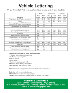


© Copyright 2026