
PDF form of documentation - PLplot
The PLplot Plotting Library i The PLplot Plotting Library Programmer's Reference Manual The PLplot Plotting Library Copyright © 1994 Geoffrey Furnish, Maurice LeBrun Copyright © 1999, 2000, 2001, 2002, 2003, 2004, 2005, 2006, 2007, 2008, 2009 Alan W. Irwin Copyright © 1999, 2000, 2001, 2002, 2003, 2004 Rafael Laboissière Copyright © 2003 Joao Cardoso Copyright © 2004 Andrew Roach Copyright © 2004,2008 Andrew Ross Copyright © 2004 Arjen Markus Copyright © 2005 Thomas J. Duck Copyright © 2008, 2009 Hezekiah M. Carty Redistribution and use in source (XML DocBook) and “compiled” forms (HTML, PDF, PostScript, DVI, TeXinfo and so forth) with or without modification, are permitted provided that the following conditions are met: 1. Redistributions of source code (XML DocBook) must retain the above copyright notice, this list of conditions and the following disclaimer as the first lines of this file unmodified. 2. Redistributions in compiled form (transformed to other DTDs, converted to HTML, PDF, PostScript, and other formats) must reproduce the above copyright notice, this list of conditions and the following disclaimer in the documentation and/or other materials provided with the distribution. Important: THIS DOCUMENTATION IS PROVIDED BY THE PLPLOT PROJECT “AS IS” AND ANY EXPRESS OR IMPLIED WARRANTIES, INCLUDING, BUT NOT LIMITED TO, THE IMPLIED WARRANTIES OF MERCHANTABILITY AND FITNESS FOR A PARTICULAR PURPOSE ARE DISCLAIMED. IN NO EVENT SHALL THE PLPLOT PROJECT BE LIABLE FOR ANY DIRECT, INDIRECT, INCIDENTAL, SPECIAL, EXEMPLARY, OR CONSEQUENTIAL DAMAGES (INCLUDING, BUT NOT LIMITED TO, PROCUREMENT OF SUBSTITUTE GOODS OR SERVICES; LOSS OF USE, DATA, OR PROFITS; OR BUSINESS INTERRUPTION) HOWEVER CAUSED AND ON ANY THEORY OF LIABILITY, WHETHER IN CONTRACT, STRICT LIABILITY, OR TORT (INCLUDING NEGLIGENCE OR OTHERWISE) ARISING IN ANY WAY OUT OF THE USE OF THIS DOCUMENTATION, EVEN IF ADVISED OF THE POSSIBILITY OF SUCH DAMAGE. Release version: 5.11.0 Release date: 2015-04-12 ii The PLplot Plotting Library iii COLLABORATORS TITLE : The PLplot Plotting Library ACTION NAME DATE SIGNATURE WRITTEN BY Maurice J. LeBrun and Geoff Furnish April 11, 2015 REVISION HISTORY NUMBER DATE DESCRIPTION NAME The PLplot Plotting Library iv Contents I 1 Introduction 1 Introduction 2 1.1 The PLplot Plotting Library . . . . . . . . . . . . . . . . . . . . . . . . . . . . . . . . . . . . . . . . . . . . . . 2 1.2 Getting a Copy of the PLplot Package . . . . . . . . . . . . . . . . . . . . . . . . . . . . . . . . . . . . . . . . 3 1.3 Installing and Using the PLplot Library . . . . . . . . . . . . . . . . . . . . . . . . . . . . . . . . . . . . . . . . 3 1.4 Organization of this Manual . . . . . . . . . . . . . . . . . . . . . . . . . . . . . . . . . . . . . . . . . . . . . . 3 1.5 Copyrights . . . . . . . . . . . . . . . . . . . . . . . . . . . . . . . . . . . . . . . . . . . . . . . . . . . . . . . 4 1.5.1 Additional Copyrights . . . . . . . . . . . . . . . . . . . . . . . . . . . . . . . . . . . . . . . . . . . . . 4 Credits . . . . . . . . . . . . . . . . . . . . . . . . . . . . . . . . . . . . . . . . . . . . . . . . . . . . . . . . . 5 1.6 II Programming 6 2 Simple Use of PLplot 7 2.1 Plotting a Simple Graph . . . . . . . . . . . . . . . . . . . . . . . . . . . . . . . . . . . . . . . . . . . . . . . . 7 2.2 Initializing PLplot . . . . . . . . . . . . . . . . . . . . . . . . . . . . . . . . . . . . . . . . . . . . . . . . . . . 7 2.3 Defining Plot Scales and Axes . . . . . . . . . . . . . . . . . . . . . . . . . . . . . . . . . . . . . . . . . . . . . 8 2.4 Labelling the Graph . . . . . . . . . . . . . . . . . . . . . . . . . . . . . . . . . . . . . . . . . . . . . . . . . . 8 2.5 Drawing the Graph . . . . . . . . . . . . . . . . . . . . . . . . . . . . . . . . . . . . . . . . . . . . . . . . . . 9 2.5.1 Drawing Points . . . . . . . . . . . . . . . . . . . . . . . . . . . . . . . . . . . . . . . . . . . . . . . . 9 2.5.2 Drawing Lines or Curves . . . . . . . . . . . . . . . . . . . . . . . . . . . . . . . . . . . . . . . . . . . 9 2.5.3 Writing Text on a Graph . . . . . . . . . . . . . . . . . . . . . . . . . . . . . . . . . . . . . . . . . . . 9 2.5.4 Area Fills . . . . . . . . . . . . . . . . . . . . . . . . . . . . . . . . . . . . . . . . . . . . . . . . . . . 10 2.5.5 More Complex Graphs . . . . . . . . . . . . . . . . . . . . . . . . . . . . . . . . . . . . . . . . . . . . 10 2.6 Finishing Up . . . . . . . . . . . . . . . . . . . . . . . . . . . . . . . . . . . . . . . . . . . . . . . . . . . . . . 10 2.7 In Case of Error . . . . . . . . . . . . . . . . . . . . . . . . . . . . . . . . . . . . . . . . . . . . . . . . . . . . 10 The PLplot Plotting Library 3 Advanced Use of PLplot v 11 3.1 Command Line Arguments . . . . . . . . . . . . . . . . . . . . . . . . . . . . . . . . . . . . . . . . . . . . . . 11 3.2 Output Devices . . . . . . . . . . . . . . . . . . . . . . . . . . . . . . . . . . . . . . . . . . . . . . . . . . . . 12 3.3 3.4 3.2.1 Driver Functions . . . . . . . . . . . . . . . . . . . . . . . . . . . . . . . . . . . . . . . . . . . . . . . 12 3.2.2 PLplot Metafiles and Plrender . . . . . . . . . . . . . . . . . . . . . . . . . . . . . . . . . . . . . . . . 14 3.2.3 Family File Output . . . . . . . . . . . . . . . . . . . . . . . . . . . . . . . . . . . . . . . . . . . . . . 16 3.2.4 Interactive Output Devices . . . . . . . . . . . . . . . . . . . . . . . . . . . . . . . . . . . . . . . . . . 16 3.2.5 Specifying the Output Device . . . . . . . . . . . . . . . . . . . . . . . . . . . . . . . . . . . . . . . . . 17 Adding FreeType Library Support to Bitmap Drivers . . . . . . . . . . . . . . . . . . . . . . . . . . . . . . . . . 18 3.3.1 Write a call back function to plot a single pixel . . . . . . . . . . . . . . . . . . . . . . . . . . . . . . . . 19 3.3.2 Initialize FreeType . . . . . . . . . . . . . . . . . . . . . . . . . . . . . . . . . . . . . . . . . . . . . . 19 3.3.3 Add A Command to redraw text (interactive drivers only) . . . . . . . . . . . . . . . . . . . . . . . . . . 20 3.3.4 Add Function Prototypes . . . . . . . . . . . . . . . . . . . . . . . . . . . . . . . . . . . . . . . . . . . 21 3.3.5 Add Closing functions . . . . . . . . . . . . . . . . . . . . . . . . . . . . . . . . . . . . . . . . . . . . . 21 View Surfaces, (Sub-)Pages, Viewports and Windows . . . . . . . . . . . . . . . . . . . . . . . . . . . . . . . . 21 3.4.1 Defining the Viewport . . . . . . . . . . . . . . . . . . . . . . . . . . . . . . . . . . . . . . . . . . . . 22 3.4.2 Defining the Window . . . . . . . . . . . . . . . . . . . . . . . . . . . . . . . . . . . . . . . . . . . . . 22 3.4.3 Annotating the Viewport . . . . . . . . . . . . . . . . . . . . . . . . . . . . . . . . . . . . . . . . . . . 23 3.4.4 Setting up a Standard Window . . . . . . . . . . . . . . . . . . . . . . . . . . . . . . . . . . . . . . . . 23 3.5 Setting Line Attributes . . . . . . . . . . . . . . . . . . . . . . . . . . . . . . . . . . . . . . . . . . . . . . . . 24 3.6 Setting the Area Fill Pattern . . . . . . . . . . . . . . . . . . . . . . . . . . . . . . . . . . . . . . . . . . . . . . 24 3.7 Setting Color . . . . . . . . . . . . . . . . . . . . . . . . . . . . . . . . . . . . . . . . . . . . . . . . . . . . . 25 3.8 3.9 3.7.1 Color Map0 . . . . . . . . . . . . . . . . . . . . . . . . . . . . . . . . . . . . . . . . . . . . . . . . . . 25 3.7.2 Color Map1 . . . . . . . . . . . . . . . . . . . . . . . . . . . . . . . . . . . . . . . . . . . . . . . . . . 25 Setting Character Attributes . . . . . . . . . . . . . . . . . . . . . . . . . . . . . . . . . . . . . . . . . . . . . . 27 3.8.1 Hershey fonts . . . . . . . . . . . . . . . . . . . . . . . . . . . . . . . . . . . . . . . . . . . . . . . . . 27 3.8.2 Unicode fonts . . . . . . . . . . . . . . . . . . . . . . . . . . . . . . . . . . . . . . . . . . . . . . . . . 28 3.8.3 FCI . . . . . . . . . . . . . . . . . . . . . . . . . . . . . . . . . . . . . . . . . . . . . . . . . . . . . . 29 3.8.4 Escape sequences in text . . . . . . . . . . . . . . . . . . . . . . . . . . . . . . . . . . . . . . . . . . . 30 3.8.5 Character size adjustment . . . . . . . . . . . . . . . . . . . . . . . . . . . . . . . . . . . . . . . . . . . 31 Three Dimensional Surface Plots . . . . . . . . . . . . . . . . . . . . . . . . . . . . . . . . . . . . . . . . . . . 31 3.10 Contour and Shade Plots . . . . . . . . . . . . . . . . . . . . . . . . . . . . . . . . . . . . . . . . . . . . . . . 33 3.10.1 Contour Plots from C . . . . . . . . . . . . . . . . . . . . . . . . . . . . . . . . . . . . . . . . . . . . . 33 3.10.2 Shade Plots from C . . . . . . . . . . . . . . . . . . . . . . . . . . . . . . . . . . . . . . . . . . . . . . 33 3.10.3 Contour Plots from the Fortran 95 interface . . . . . . . . . . . . . . . . . . . . . . . . . . . . . . . . . 33 3.10.4 Shade Plots from the Fortran 95 interface . . . . . . . . . . . . . . . . . . . . . . . . . . . . . . . . . . 33 3.11 Legends and color bars . . . . . . . . . . . . . . . . . . . . . . . . . . . . . . . . . . . . . . . . . . . . . . . . 34 4 Deploying programs that use PLplot 35 The PLplot Plotting Library vi 5 38 The PLplot Display Driver Family 5.1 The Xwin Driver (X-Windows) . . . . . . . . . . . . . . . . . . . . . . . . . . . . . . . . . . . . . . . . . . . . 38 5.2 The Tk Driver . . . . . . . . . . . . . . . . . . . . . . . . . . . . . . . . . . . . . . . . . . . . . . . . . . . . . 38 5.3 The AquaTerm Driver (Mac OS X) . . . . . . . . . . . . . . . . . . . . . . . . . . . . . . . . . . . . . . . . . . 38 5.4 The wxWidgets Driver (Linux, Mac OS X, Windows) . . . . . . . . . . . . . . . . . . . . . . . . . . . . . . . . 39 5.4.1 6 The PLplot Output Driver Family 40 6.1 The GD Driver . . . . . . . . . . . . . . . . . . . . . . . . . . . . . . . . . . . . . . . . . . . . . . . . . . . . 40 6.2 The PDF Driver . . . . . . . . . . . . . . . . . . . . . . . . . . . . . . . . . . . . . . . . . . . . . . . . . . . . 40 6.3 The PostScript Driver . . . . . . . . . . . . . . . . . . . . . . . . . . . . . . . . . . . . . . . . . . . . . . . . . 41 6.4 The TrueType PostScript Driver . . . . . . . . . . . . . . . . . . . . . . . . . . . . . . . . . . . . . . . . . . . 41 6.5 The LaTeX PostScript Driver . . . . . . . . . . . . . . . . . . . . . . . . . . . . . . . . . . . . . . . . . . . . . 41 6.6 The SVG Driver . . . . . . . . . . . . . . . . . . . . . . . . . . . . . . . . . . . . . . . . . . . . . . . . . . . . 42 III 7 wxWidgets Driver Basics . . . . . . . . . . . . . . . . . . . . . . . . . . . . . . . . . . . . . . . . . . . 39 Language Bindings Ada Language 43 44 7.1 Overview . . . . . . . . . . . . . . . . . . . . . . . . . . . . . . . . . . . . . . . . . . . . . . . . . . . . . . . 44 7.2 The Bindings . . . . . . . . . . . . . . . . . . . . . . . . . . . . . . . . . . . . . . . . . . . . . . . . . . . . . 44 7.2.1 Thin Binding . . . . . . . . . . . . . . . . . . . . . . . . . . . . . . . . . . . . . . . . . . . . . . . . . 44 7.2.2 The Thick Bindings . . . . . . . . . . . . . . . . . . . . . . . . . . . . . . . . . . . . . . . . . . . . . . 45 7.2.3 Standard Thick Binding Using Enhanced Names . . . . . . . . . . . . . . . . . . . . . . . . . . . . . . . 45 7.2.4 Thick Binding Using Traditional Names . . . . . . . . . . . . . . . . . . . . . . . . . . . . . . . . . . . 46 7.3 The Examples . . . . . . . . . . . . . . . . . . . . . . . . . . . . . . . . . . . . . . . . . . . . . . . . . . . . . 46 7.4 Obtaining the Software . . . . . . . . . . . . . . . . . . . . . . . . . . . . . . . . . . . . . . . . . . . . . . . . 46 7.5 7.6 7.4.1 Obtaining an Ada compiler . . . . . . . . . . . . . . . . . . . . . . . . . . . . . . . . . . . . . . . . . . 46 7.4.2 Download and install PLplot . . . . . . . . . . . . . . . . . . . . . . . . . . . . . . . . . . . . . . . . . 46 7.4.3 The Ada bindings to PLplot . . . . . . . . . . . . . . . . . . . . . . . . . . . . . . . . . . . . . . . . . . 46 How to use the Ada bindings . . . . . . . . . . . . . . . . . . . . . . . . . . . . . . . . . . . . . . . . . . . . . 47 7.5.1 Ada 95 versus Ada 2005 . . . . . . . . . . . . . . . . . . . . . . . . . . . . . . . . . . . . . . . . . . . 47 7.5.2 GNAT versus non-GNAT . . . . . . . . . . . . . . . . . . . . . . . . . . . . . . . . . . . . . . . . . . . 47 7.5.3 Sample command line project . . . . . . . . . . . . . . . . . . . . . . . . . . . . . . . . . . . . . . . . . 47 Unique Features of the Ada bindings . . . . . . . . . . . . . . . . . . . . . . . . . . . . . . . . . . . . . . . . . 48 7.6.1 High-level features for simplified plotting . . . . . . . . . . . . . . . . . . . . . . . . . . . . . . . . . . . 48 7.6.1.1 Foreground-background control . . . . . . . . . . . . . . . . . . . . . . . . . . . . . . . . . . 48 7.6.1.1.1 7.6.1.2 Draw_On_Black, Draw_On_White . . . . . . . . . . . . . . . . . . . . . . . . . . . 48 Simple Plotters . . . . . . . . . . . . . . . . . . . . . . . . . . . . . . . . . . . . . . . . . . . 49 7.6.1.2.1 Multiplot_Pairs . . . . . . . . . . . . . . . . . . . . . . . . . . . . . . . . . . . . . 49 The PLplot Plotting Library vii 7.6.1.2.2 Simple_Plot . . . . . . . . . . . . . . . . . . . . . . . . . . . . . . . . . . . . . . . 49 7.6.1.2.3 Simple_Plot_Log_X . . . . . . . . . . . . . . . . . . . . . . . . . . . . . . . . . . . 49 7.6.1.2.4 Simple_Plot_Log_Y . . . . . . . . . . . . . . . . . . . . . . . . . . . . . . . . . . . 49 7.6.1.2.5 Simple_Plot_Log_XY . . . . . . . . . . . . . . . . . . . . . . . . . . . . . . . . . . 49 7.6.1.2.6 Simple_Plot_Pairs . . . . . . . . . . . . . . . . . . . . . . . . . . . . . . . . . . . . 49 7.6.1.2.7 Single_Plot . . . . . . . . . . . . . . . . . . . . . . . . . . . . . . . . . . . . . . . 49 7.6.1.2.8 Simple_Contour . . . . . . . . . . . . . . . . . . . . . . . . . . . . . . . . . . . . . 49 7.6.1.2.9 Simple_Mesh_3D . . . . . . . . . . . . . . . . . . . . . . . . . . . . . . . . . . . . 49 7.6.1.2.10 Simple_Surface_3D . . . . . . . . . . . . . . . . . . . . . . . . . . . . . . . . . . . 49 7.6.1.3 7.7 7.6.2 Integer Options Given Ada Names . . . . . . . . . . . . . . . . . . . . . . . . . . . . . . . . . . . . . . 50 7.6.3 One-offs . . . . . . . . . . . . . . . . . . . . . . . . . . . . . . . . . . . . . . . . . . . . . . . . . . . . 52 Parts That Retain a C Flavor . . . . . . . . . . . . . . . . . . . . . . . . . . . . . . . . . . . . . . . . . . . . . 52 7.7.1 7.8 7.9 Simple color map manipulations . . . . . . . . . . . . . . . . . . . . . . . . . . . . . . . . . . 50 Map-drawing . . . . . . . . . . . . . . . . . . . . . . . . . . . . . . . . . . . . . . . . . . . . . . . . . 52 Known Variances . . . . . . . . . . . . . . . . . . . . . . . . . . . . . . . . . . . . . . . . . . . . . . . . . . . 52 7.8.1 Documentation . . . . . . . . . . . . . . . . . . . . . . . . . . . . . . . . . . . . . . . . . . . . . . . . 52 7.8.2 API . . . . . . . . . . . . . . . . . . . . . . . . . . . . . . . . . . . . . . . . . . . . . . . . . . . . . . 53 Compilation notes . . . . . . . . . . . . . . . . . . . . . . . . . . . . . . . . . . . . . . . . . . . . . . . . . . . 53 7.9.1 Ada 95 Versus Ada 2005 . . . . . . . . . . . . . . . . . . . . . . . . . . . . . . . . . . . . . . . . . . . 53 7.9.2 GNAT Dependence . . . . . . . . . . . . . . . . . . . . . . . . . . . . . . . . . . . . . . . . . . . . . . 53 7.9.3 PLplot_Auxiliary . . . . . . . . . . . . . . . . . . . . . . . . . . . . . . . . . . . . . . . . . . . . . . . 53 7.10 Notes for Apple Macintosh OS X users . . . . . . . . . . . . . . . . . . . . . . . . . . . . . . . . . . . . . . . . 53 7.10.1 Using Apple's Xcode IDE . . . . . . . . . . . . . . . . . . . . . . . . . . . . . . . . . . . . . . . . . . . 53 7.10.2 AquaTerm . . . . . . . . . . . . . . . . . . . . . . . . . . . . . . . . . . . . . . . . . . . . . . . . . . . 54 7.10.3 X11 . . . . . . . . . . . . . . . . . . . . . . . . . . . . . . . . . . . . . . . . . . . . . . . . . . . . . . 54 7.10.4 GNAT for OS X . . . . . . . . . . . . . . . . . . . . . . . . . . . . . . . . . . . . . . . . . . . . . . . 54 8 C Language 55 9 A C++ Interface for PLplot 57 9.1 Motivation for the C++ Interface . . . . . . . . . . . . . . . . . . . . . . . . . . . . . . . . . . . . . . . . . . . 57 9.2 Design of the PLplot C++ Interface . . . . . . . . . . . . . . . . . . . . . . . . . . . . . . . . . . . . . . . . . . 58 9.2.1 Stream/Object Identity . . . . . . . . . . . . . . . . . . . . . . . . . . . . . . . . . . . . . . . . . . . . 58 9.2.2 Namespace Management . . . . . . . . . . . . . . . . . . . . . . . . . . . . . . . . . . . . . . . . . . . 58 9.2.3 Abstraction of Data Layout . . . . . . . . . . . . . . . . . . . . . . . . . . . . . . . . . . . . . . . . . . 58 9.2.4 Callbacks and Shades . . . . . . . . . . . . . . . . . . . . . . . . . . . . . . . . . . . . . . . . . . . . . 59 9.2.5 Collapsing the API . . . . . . . . . . . . . . . . . . . . . . . . . . . . . . . . . . . . . . . . . . . . . . 59 9.3 Specializing the PLplot C++ Interface . . . . . . . . . . . . . . . . . . . . . . . . . . . . . . . . . . . . . . . . 59 9.4 Status of the C++ Interface . . . . . . . . . . . . . . . . . . . . . . . . . . . . . . . . . . . . . . . . . . . . . . 60 The PLplot Plotting Library viii 10 Fortran 95 Language 61 11 OCaml Language 64 11.1 Overview . . . . . . . . . . . . . . . . . . . . . . . . . . . . . . . . . . . . . . . . . . . . . . . . . . . . . . . 64 11.2 The Bindings . . . . . . . . . . . . . . . . . . . . . . . . . . . . . . . . . . . . . . . . . . . . . . . . . . . . . 64 11.2.1 Core Binding . . . . . . . . . . . . . . . . . . . . . . . . . . . . . . . . . . . . . . . . . . . . . . . . . 64 11.2.2 OCaml-specific variations to the core PLplot API . . . . . . . . . . . . . . . . . . . . . . . . . . . . . . 65 11.2.3 OCaml high level 2D plotting API . . . . . . . . . . . . . . . . . . . . . . . . . . . . . . . . . . . . . . 65 11.3 The Examples . . . . . . . . . . . . . . . . . . . . . . . . . . . . . . . . . . . . . . . . . . . . . . . . . . . . . 65 11.4 Obtaining the Software . . . . . . . . . . . . . . . . . . . . . . . . . . . . . . . . . . . . . . . . . . . . . . . . 65 11.4.1 Obtaining the OCaml compiler . . . . . . . . . . . . . . . . . . . . . . . . . . . . . . . . . . . . . . . . 65 11.5 How to use the OCaml bindings . . . . . . . . . . . . . . . . . . . . . . . . . . . . . . . . . . . . . . . . . . . . 65 11.5.1 How to setup findlib for use with the OCaml bindings . . . . . . . . . . . . . . . . . . . . . . . . . . . . 65 11.5.2 Sample command line project (core API) . . . . . . . . . . . . . . . . . . . . . . . . . . . . . . . . . . . 66 11.5.3 Sample command line project (OCaml-specific API) . . . . . . . . . . . . . . . . . . . . . . . . . . . . . 66 11.5.4 Sample toplevel project . . . . . . . . . . . . . . . . . . . . . . . . . . . . . . . . . . . . . . . . . . . . 67 11.6 Known Issues . . . . . . . . . . . . . . . . . . . . . . . . . . . . . . . . . . . . . . . . . . . . . . . . . . . . . 67 12 Using PLplot from Perl 68 13 Using PLplot from Python 70 14 Using PLplot from Tcl 71 14.1 Motivation for the Tcl Interface to PLplot . . . . . . . . . . . . . . . . . . . . . . . . . . . . . . . . . . . . . . . 71 14.2 Overview of the Tcl Language Binding . . . . . . . . . . . . . . . . . . . . . . . . . . . . . . . . . . . . . . . . 72 14.3 The PLplot Tcl Matrix Extension . . . . . . . . . . . . . . . . . . . . . . . . . . . . . . . . . . . . . . . . . . . 73 14.3.1 Using Tcl Matrices from Tcl . . . . . . . . . . . . . . . . . . . . . . . . . . . . . . . . . . . . . . . . . 74 14.3.2 Using Tcl Matrices from C . . . . . . . . . . . . . . . . . . . . . . . . . . . . . . . . . . . . . . . . . . 75 14.3.3 Using Tcl Matrices from C++ . . . . . . . . . . . . . . . . . . . . . . . . . . . . . . . . . . . . . . . . . 75 14.3.4 Extending the Tcl Matrix facility . . . . . . . . . . . . . . . . . . . . . . . . . . . . . . . . . . . . . . . 76 14.4 Contouring and Shading from Tcl . . . . . . . . . . . . . . . . . . . . . . . . . . . . . . . . . . . . . . . . . . . 77 14.4.1 Drawing a Contour Plot from Tcl . . . . . . . . . . . . . . . . . . . . . . . . . . . . . . . . . . . . . . . 77 14.4.2 Drawing a Shaded Plot from Tcl . . . . . . . . . . . . . . . . . . . . . . . . . . . . . . . . . . . . . . . 78 14.5 Understanding the Performance Characteristics of Tcl . . . . . . . . . . . . . . . . . . . . . . . . . . . . . . . . 78 15 Building an Extended WISH 80 15.1 Introduction to Tcl . . . . . . . . . . . . . . . . . . . . . . . . . . . . . . . . . . . . . . . . . . . . . . . . . . . 80 15.1.1 Motivation for Tcl . . . . . . . . . . . . . . . . . . . . . . . . . . . . . . . . . . . . . . . . . . . . . . . 80 15.1.2 Capabilities of Tcl . . . . . . . . . . . . . . . . . . . . . . . . . . . . . . . . . . . . . . . . . . . . . . . 80 15.1.3 Acquiring Tcl . . . . . . . . . . . . . . . . . . . . . . . . . . . . . . . . . . . . . . . . . . . . . . . . . 81 15.2 Introduction to Tk . . . . . . . . . . . . . . . . . . . . . . . . . . . . . . . . . . . . . . . . . . . . . . . . . . . 81 The PLplot Plotting Library ix 15.3 Introduction to [incr Tcl] . . . . . . . . . . . . . . . . . . . . . . . . . . . . . . . . . . . . . . . . . . . . . . . 82 15.4 PLplot Extensions to Tcl . . . . . . . . . . . . . . . . . . . . . . . . . . . . . . . . . . . . . . . . . . . . . . . . 82 15.5 Custom Extensions to Tcl . . . . . . . . . . . . . . . . . . . . . . . . . . . . . . . . . . . . . . . . . . . . . . . 82 15.5.1 WISH Construction . . . . . . . . . . . . . . . . . . . . . . . . . . . . . . . . . . . . . . . . . . . . . . 83 15.5.2 WISH Linking . . . . . . . . . . . . . . . . . . . . . . . . . . . . . . . . . . . . . . . . . . . . . . . . 84 15.5.3 WISH Programming . . . . . . . . . . . . . . . . . . . . . . . . . . . . . . . . . . . . . . . . . . . . . 84 16 Embedding Plots in Graphical User Interfaces 85 IV 86 Reference 17 Bibliography 87 17.1 References . . . . . . . . . . . . . . . . . . . . . . . . . . . . . . . . . . . . . . . . . . . . . . . . . . . . . . . 87 18 The Common API for PLplot 88 18.1 pl_setcontlabelformat: Set format of numerical label for contours . . . . . . . . . . . . . . . . . . . . . 89 18.2 pl_setcontlabelparam: Set parameters of contour labelling other than format of numerical label . . . . . . 89 18.3 pladv: Advance the (sub-)page . . . . . . . . . . . . . . . . . . . . . . . . . . . . . . . . . . . . . . . . . . . 89 18.4 plarc: Draw a circular or elliptical arc . . . . . . . . . . . . . . . . . . . . . . . . . . . . . . . . . . . . . . . 90 18.5 plaxes: Draw a box with axes, etc. with arbitrary origin . . . . . . . . . . . . . . . . . . . . . . . . . . . . . 90 18.6 plbin: Plot a histogram from binned data . . . . . . . . . . . . . . . . . . . . . . . . . . . . . . . . . . . . . 91 18.7 plbop: Begin a new page . . . . . . . . . . . . . . . . . . . . . . . . . . . . . . . . . . . . . . . . . . . . . . 92 18.8 plbox: Draw a box with axes, etc . . . . . . . . . . . . . . . . . . . . . . . . . . . . . . . . . . . . . . . . . . 92 18.9 plbox3: Draw a box with axes, etc, in 3-d . . . . . . . . . . . . . . . . . . . . . . . . . . . . . . . . . . . . . 93 18.10 plbtime: Calculate broken-down time from continuous time for the current stream . . . . . . . . . . . . . . . 95 18.11 plcalc_world: Calculate world coordinates and corresponding window index from relative device coordinates 95 18.12 plclear: Clear current (sub)page . . . . . . . . . . . . . . . . . . . . . . . . . . . . . . . . . . . . . . . . . 96 18.13 plcol0: Set color, cmap0 . . . . . . . . . . . . . . . . . . . . . . . . . . . . . . . . . . . . . . . . . . . . . 96 18.14 plcol1: Set color, cmap1 . . . . . . . . . . . . . . . . . . . . . . . . . . . . . . . . . . . . . . . . . . . . . 97 18.15 plcolorbar: Plot color bar for image, shade or gradient plots . . . . . . . . . . . . . . . . . . . . . . . . . . 97 18.16 plconfigtime: Configure the transformation between continuous and broken-down time for the current stream 99 18.17 plcont: Contour plot . . . . . . . . . . . . . . . . . . . . . . . . . . . . . . . . . . . . . . . . . . . . . . . . 100 18.18 plcpstrm: Copy state parameters from the reference stream to the current stream . . . . . . . . . . . . . . . . 101 18.19 plctime: Calculate continuous time from broken-down time for the current stream . . . . . . . . . . . . . . . 101 18.20 plend: End plotting session . . . . . . . . . . . . . . . . . . . . . . . . . . . . . . . . . . . . . . . . . . . . . 102 18.21 plend1: End plotting session for current stream . . . . . . . . . . . . . . . . . . . . . . . . . . . . . . . . . . 102 18.22 plenv0: Same as plenv but if in multiplot mode does not advance the subpage, instead clears it . . . . . . . . . . . 102 18.23 plenv: Set up standard window and draw box . . . . . . . . . . . . . . . . . . . . . . . . . . . . . . . . . . . 104 18.24 pleop: Eject current page . . . . . . . . . . . . . . . . . . . . . . . . . . . . . . . . . . . . . . . . . . . . . 105 18.25 plerrx: Draw x error bar . . . . . . . . . . . . . . . . . . . . . . . . . . . . . . . . . . . . . . . . . . . . . 105 The PLplot Plotting Library 18.26 plerry: Draw y error bar x . . . . . . . . . . . . . . . . . . . . . . . . . . . . . . . . . . . . . . . . . . . . . 106 18.27 plfamadv: Advance to the next family file on the next new page . . . . . . . . . . . . . . . . . . . . . . . . . 106 18.28 plfill: Draw filled polygon . . . . . . . . . . . . . . . . . . . . . . . . . . . . . . . . . . . . . . . . . . . . 106 18.29 plfill3: Draw filled polygon in 3D . . . . . . . . . . . . . . . . . . . . . . . . . . . . . . . . . . . . . . . . 107 18.30 plflush: Flushes the output stream . . . . . . . . . . . . . . . . . . . . . . . . . . . . . . . . . . . . . . . . 107 18.31 plfont: Set character font . . . . . . . . . . . . . . . . . . . . . . . . . . . . . . . . . . . . . . . . . . . . . 107 18.32 plfontld: Load character font . . . . . . . . . . . . . . . . . . . . . . . . . . . . . . . . . . . . . . . . . . 108 18.33 plgchr: Get character default height and current (scaled) height . . . . . . . . . . . . . . . . . . . . . . . . . 108 18.34 plgcmap1_range: Get the cmap1 argument range for continuous color plots . . . . . . . . . . . . . . . . . . 108 18.35 plgcol0: Returns 8-bit RGB values for given color index from cmap0 . . . . . . . . . . . . . . . . . . . . . . 108 18.36 plgcol0a: Returns 8-bit RGB values and double alpha transparency value for given color index from cmap0 . . 109 18.37 plgcolbg: Returns the background color (cmap0[0]) by 8-bit RGB value . . . . . . . . . . . . . . . . . . . . 109 18.38 plgcolbga: Returns the background color (cmap0[0]) by 8-bit RGB value and double alpha transparency value 18.39 plgcompression: Get the current device-compression setting 109 . . . . . . . . . . . . . . . . . . . . . . . . . 110 18.40 plgdev: Get the current device (keyword) name . . . . . . . . . . . . . . . . . . . . . . . . . . . . . . . . . . 110 18.41 plgdidev: Get parameters that define current device-space window 18.42 plgdiori: Get plot orientation . . . . . . . . . . . . . . . . . . . . . . . 110 . . . . . . . . . . . . . . . . . . . . . . . . . . . . . . . . . . . . . . . . . . 110 18.43 plgdiplt: Get parameters that define current plot-space window . . . . . . . . . . . . . . . . . . . . . . . . . 111 18.44 plgdrawmode: Get drawing mode (depends on device support!) . . . . . . . . . . . . . . . . . . . . . . . . . 111 18.45 plgfam: Get family file parameters . . . . . . . . . . . . . . . . . . . . . . . . . . . . . . . . . . . . . . . . . 111 18.46 plgfci: Get FCI (font characterization integer) . . . . . . . . . . . . . . . . . . . . . . . . . . . . . . . . . . 111 18.47 plgfnam: Get output file name . . . . . . . . . . . . . . . . . . . . . . . . . . . . . . . . . . . . . . . . . . . 112 18.48 plgfont: Get family, style and weight of the current font . . . . . . . . . . . . . . . . . . . . . . . . . . . . . 112 18.49 plglevel: Get the (current) run level . . . . . . . . . . . . . . . . . . . . . . . . . . . . . . . . . . . . . . . 112 18.50 plgpage: Get page parameters . . . . . . . . . . . . . . . . . . . . . . . . . . . . . . . . . . . . . . . . . . . 113 18.51 plgra: Switch to graphics screen . . . . . . . . . . . . . . . . . . . . . . . . . . . . . . . . . . . . . . . . . . 113 18.52 plgradient: Draw linear gradient inside polygon . . . . . . . . . . . . . . . . . . . . . . . . . . . . . . . . 113 18.53 plgriddata: Grid data from irregularly sampled data . . . . . . . . . . . . . . . . . . . . . . . . . . . . . . 114 18.54 plgspa: Get current subpage parameters . . . . . . . . . . . . . . . . . . . . . . . . . . . . . . . . . . . . . . 115 18.55 plgstrm: Get current stream number . . . . . . . . . . . . . . . . . . . . . . . . . . . . . . . . . . . . . . . 115 18.56 plgver: Get the current library version number . . . . . . . . . . . . . . . . . . . . . . . . . . . . . . . . . . 115 18.57 plgvpd: Get viewport limits in normalized device coordinates . . . . . . . . . . . . . . . . . . . . . . . . . . . 115 18.58 plgvpw: Get viewport limits in world coordinates . . . . . . . . . . . . . . . . . . . . . . . . . . . . . . . . . 116 18.59 plgxax: Get x axis parameters . . . . . . . . . . . . . . . . . . . . . . . . . . . . . . . . . . . . . . . . . . . 116 18.60 plgyax: Get y axis parameters . . . . . . . . . . . . . . . . . . . . . . . . . . . . . . . . . . . . . . . . . . . 116 18.61 plgzax: Get z axis parameters . . . . . . . . . . . . . . . . . . . . . . . . . . . . . . . . . . . . . . . . . . . 117 18.62 plhist: Plot a histogram from unbinned data . . . . . . . . . . . . . . . . . . . . . . . . . . . . . . . . . . . 117 18.63 plhlsrgb: Convert HLS color to RGB . . . . . . . . . . . . . . . . . . . . . . . . . . . . . . . . . . . . . . 118 18.64 plimagefr: Plot a 2D matrix using cmap1 . . . . . . . . . . . . . . . . . . . . . . . . . . . . . . . . . . . . 118 The PLplot Plotting Library xi 18.65 plimage: Plot a 2D matrix using cmap1 with automatic colour adjustment . . . . . . . . . . . . . . . . . . . . 119 18.66 plinit: Initialize PLplot . . . . . . . . . . . . . . . . . . . . . . . . . . . . . . . . . . . . . . . . . . . . . . 119 18.67 pljoin: Draw a line between two points . . . . . . . . . . . . . . . . . . . . . . . . . . . . . . . . . . . . . . 119 18.68 pllab: Simple routine to write labels . . . . . . . . . . . . . . . . . . . . . . . . . . . . . . . . . . . . . . . . 120 18.69 pllegend: Plot legend using discretely annotated filled boxes, lines, and/or lines of symbols . . . . . . . . . . . 120 18.70 pllightsource: Sets the 3D position of the light source . . . . . . . . . . . . . . . . . . . . . . . . . . . . 122 18.71 plline: Draw a line . . . . . . . . . . . . . . . . . . . . . . . . . . . . . . . . . . . . . . . . . . . . . . . . 122 18.72 plline3: Draw a line in 3 space . . . . . . . . . . . . . . . . . . . . . . . . . . . . . . . . . . . . . . . . . . 123 18.73 pllsty: Select line style . . . . . . . . . . . . . . . . . . . . . . . . . . . . . . . . . . . . . . . . . . . . . . 123 18.74 plmap: Plot continental outline or shapefile data in world coordinates . . . . . . . . . . . . . . . . . . . . . . . 123 18.75 plmapfill: Plot all or a subset of Shapefile data, filling the polygons . . . . . . . . . . . . . . . . . . . . . . . 124 18.76 plmapline: Plot all or a subset of Shapefile data using lines in world coordinates . . . . . . . . . . . . . . . . 125 18.77 plmapstring: Plot all or a subset of Shapefile data using strings or points in world coordinates . . . . . . . . . 125 18.78 plmaptex: Draw text at points defined by Shapefile data in world coordinates . . . . . . . . . . . . . . . . . . 126 18.79 plmeridians: Plot latitude and longitude lines . . . . . . . . . . . . . . . . . . . . . . . . . . . . . . . . . . 127 18.80 plmesh: Plot surface mesh . . . . . . . . . . . . . . . . . . . . . . . . . . . . . . . . . . . . . . . . . . . . . 127 18.81 plmeshc: Magnitude colored plot surface mesh with contour . . . . . . . . . . . . . . . . . . . . . . . . . . . 128 18.82 plmkstrm: Creates a new stream and makes it the default . . . . . . . . . . . . . . . . . . . . . . . . . . . . . 129 18.83 plmtex: Write text relative to viewport boundaries . . . . . . . . . . . . . . . . . . . . . . . . . . . . . . . . 129 18.84 plmtex3: Write text relative to viewport boundaries in 3D plots . . . . . . . . . . . . . . . . . . . . . . . . . . 130 18.85 plot3d: Plot 3-d surface plot . . . . . . . . . . . . . . . . . . . . . . . . . . . . . . . . . . . . . . . . . . . . 130 18.86 plot3dc: Magnitude colored plot surface with contour . . . . . . . . . . . . . . . . . . . . . . . . . . . . . . 131 18.87 plot3dcl: Magnitude colored plot surface with contour for z[x][y] with y index limits . . . . . . . . . . . . . . 132 18.88 plparseopts: Parse command-line arguments . . . . . . . . . . . . . . . . . . . . . . . . . . . . . . . . . . 133 18.89 plpat: Set area fill pattern . . . . . . . . . . . . . . . . . . . . . . . . . . . . . . . . . . . . . . . . . . . . . 133 18.90 plpath: Draw a line between two points, accounting for coordinate transforms . . . . . . . . . . . . . . . . . . 134 18.91 plpoin: Plot a glyph at the specified points . . . . . . . . . . . . . . . . . . . . . . . . . . . . . . . . . . . . 134 18.92 plpoin3: Plot a glyph at the specified 3D points . . . . . . . . . . . . . . . . . . . . . . . . . . . . . . . . . . 135 18.93 plpoly3: Draw a polygon in 3 space . . . . . . . . . . . . . . . . . . . . . . . . . . . . . . . . . . . . . . . . 135 18.94 plprec: Set precision in numeric labels . . . . . . . . . . . . . . . . . . . . . . . . . . . . . . . . . . . . . . 136 18.95 plpsty: Select area fill pattern . . . . . . . . . . . . . . . . . . . . . . . . . . . . . . . . . . . . . . . . . . . 136 18.96 plptex: Write text inside the viewport . . . . . . . . . . . . . . . . . . . . . . . . . . . . . . . . . . . . . . . 136 18.97 plptex3: Write text inside the viewport of a 3D plot . . . . . . . . . . . . . . . . . . . . . . . . . . . . . . . 137 18.98 plrandd: Random number generator returning a real random number in the range [0,1] . . . . . . . . . . . . . 137 18.99 plreplot: Replays contents of plot buffer to current device/file 18.100plrgbhls: Convert RGB color to HLS . . . . . . . . . . . . . . . . . . . . . . . . . 137 . . . . . . . . . . . . . . . . . . . . . . . . . . . . . . . . . . . . . . 138 18.101plschr: Set character size . . . . . . . . . . . . . . . . . . . . . . . . . . . . . . . . . . . . . . . . . . . . . 138 18.102plscmap0: Set cmap0 colors by 8-bit RGB values . . . . . . . . . . . . . . . . . . . . . . . . . . . . . . . . . 138 18.103plscmap0a: Set cmap0 colors by 8-bit RGB values and double alpha transparency value . . . . . . . . . . . . . 139 The PLplot Plotting Library xii 18.104plscmap0n: Set number of colors in cmap0 . . . . . . . . . . . . . . . . . . . . . . . . . . . . . . . . . . . . 139 18.105plscmap1_range: Set the cmap1 argument range for continuous color plots . . . . . . . . . . . . . . . . . . 139 18.106plscmap1: Set cmap1 colors using 8-bit RGB values . . . . . . . . . . . . . . . . . . . . . . . . . . . . . . . 140 18.107plscmap1a: Set cmap1 colors using 8-bit RGB values and double alpha transparency values . . . . . . . . . . . 140 18.108plscmap1l: Set cmap1 colors using a piece-wise linear relationship . . . . . . . . . . . . . . . . . . . . . . . 140 18.109plscmap1la: Set cmap1 colors and alpha transparency using a piece-wise linear relationship . . . . . . . . . . 141 18.110plscmap1n: Set number of colors in cmap1 . . . . . . . . . . . . . . . . . . . . . . . . . . . . . . . . . . . . 142 18.111plscol0: Set 8-bit RGB values for given cmap0 color index . . . . . . . . . . . . . . . . . . . . . . . . . . . 142 18.112plscol0a: Set 8-bit RGB values and double alpha transparency value for given cmap0 color index . . . . . . . 143 18.113plscolbg: Set the background color by 8-bit RGB value . . . . . . . . . . . . . . . . . . . . . . . . . . . . . 143 18.114plscolbga: Set the background color by 8-bit RGB value and double alpha transparency value. . . . . . . . . . 143 18.115plscolor: Used to globally turn color output on/off . . . . . . . . . . . . . . . . . . . . . . . . . . . . . . . 144 18.116plscompression: Set device-compression level . . . . . . . . . . . . . . . . . . . . . . . . . . . . . . . . . 144 18.117plsdev: Set the device (keyword) name . . . . . . . . . . . . . . . . . . . . . . . . . . . . . . . . . . . . . . 144 18.118plsdidev: Set parameters that define current device-space window . . . . . . . . . . . . . . . . . . . . . . . . 144 18.119plsdimap: Set up transformation from metafile coordinates . . . . . . . . . . . . . . . . . . . . . . . . . . . . 145 18.120plsdiori: Set plot orientation . . . . . . . . . . . . . . . . . . . . . . . . . . . . . . . . . . . . . . . . . . . 145 18.121plsdiplt: Set parameters that define current plot-space window . . . . . . . . . . . . . . . . . . . . . . . . . 146 18.122plsdiplz: Set parameters incrementally (zoom mode) that define current plot-space window . . . . . . . . . . 146 18.123plsdrawmode: Set drawing mode (depends on device support!) 18.124plseed: Set seed for internal random number generator. . . . . . . . . . . . . . . . . . . . . . . . . . 146 . . . . . . . . . . . . . . . . . . . . . . . . . . . . . 147 18.125plsesc: Set the escape character for text strings . . . . . . . . . . . . . . . . . . . . . . . . . . . . . . . . . . 147 18.126plsetopt: Set any command-line option . . . . . . . . . . . . . . . . . . . . . . . . . . . . . . . . . . . . . 147 18.127plsfam: Set family file parameters . . . . . . . . . . . . . . . . . . . . . . . . . . . . . . . . . . . . . . . . . 148 18.128plsfci: Set FCI (font characterization integer) . . . . . . . . . . . . . . . . . . . . . . . . . . . . . . . . . . 148 18.129plsfnam: Set output file name . . . . . . . . . . . . . . . . . . . . . . . . . . . . . . . . . . . . . . . . . . . 148 18.130plsfont: Set family, style and weight of the current font . . . . . . . . . . . . . . . . . . . . . . . . . . . . . 148 18.131plshades: Shade regions on the basis of value . . . . . . . . . . . . . . . . . . . . . . . . . . . . . . . . . . 149 18.132plshade: Shade individual region on the basis of value . . . . . . . . . . . . . . . . . . . . . . . . . . . . . . 150 18.133plshade1: Shade individual region on the basis of value . . . . . . . . . . . . . . . . . . . . . . . . . . . . . 151 18.134plslabelfunc: Assign a function to use for generating custom axis labels 18.135plsmaj: Set length of major ticks . . . . . . . . . . . . . . . . . . . 153 . . . . . . . . . . . . . . . . . . . . . . . . . . . . . . . . . . . . . . . . . 153 18.136plsmem: Set the memory area to be plotted (RGB) . . . . . . . . . . . . . . . . . . . . . . . . . . . . . . . . . 153 18.137plsmema: Set the memory area to be plotted (RGBA) . . . . . . . . . . . . . . . . . . . . . . . . . . . . . . . 154 18.138plsmin: Set length of minor ticks . . . . . . . . . . . . . . . . . . . . . . . . . . . . . . . . . . . . . . . . . 154 18.139plsori: Set orientation . . . . . . . . . . . . . . . . . . . . . . . . . . . . . . . . . . . . . . . . . . . . . . . 154 18.140plspage: Set page parameters . . . . . . . . . . . . . . . . . . . . . . . . . . . . . . . . . . . . . . . . . . . 154 18.141plspal0: Set the colors for color table 0 from a cmap0 file . . . . . . . . . . . . . . . . . . . . . . . . . . . . 155 18.142plspal1: Set the palette for cmap1 using the specified cmap1*.pal format file . . . . . . . . . . . . . . . . . . 155 The PLplot Plotting Library xiii 18.143plspause: Set the pause (on end-of-page) status . . . . . . . . . . . . . . . . . . . . . . . . . . . . . . . . . 155 18.144plsstrm: Set current output stream . . . . . . . . . . . . . . . . . . . . . . . . . . . . . . . . . . . . . . . . 156 18.145plssub: Set the number of subpages in x and y . . . . . . . . . . . . . . . . . . . . . . . . . . . . . . . . . . 156 18.146plssym: Set symbol size . . . . . . . . . . . . . . . . . . . . . . . . . . . . . . . . . . . . . . . . . . . . . . 156 18.147plstar: Initialization . . . . . . . . . . . . . . . . . . . . . . . . . . . . . . . . . . . . . . . . . . . . . . . . 156 18.148plstart: Initialization . . . . . . . . . . . . . . . . . . . . . . . . . . . . . . . . . . . . . . . . . . . . . . . 157 18.149plstransform: Set a global coordinate transform function . . . . . . . . . . . . . . . . . . . . . . . . . . . 157 18.150plstring: Plot a glyph at the specified points . . . . . . . . . . . . . . . . . . . . . . . . . . . . . . . . . . . 157 18.151plstring3: Plot a glyph at the specified 3D points . . . . . . . . . . . . . . . . . . . . . . . . . . . . . . . . 158 18.152plstripa: Add a point to a strip chart 18.153plstripc: Create a 4-pen strip chart . . . . . . . . . . . . . . . . . . . . . . . . . . . . . . . . . . . . . . 158 . . . . . . . . . . . . . . . . . . . . . . . . . . . . . . . . . . . . . . . 159 18.154plstripd: Deletes and releases memory used by a strip chart . . . . . . . . . . . . . . . . . . . . . . . . . . . 160 18.155plstyl: Set line style . . . . . . . . . . . . . . . . . . . . . . . . . . . . . . . . . . . . . . . . . . . . . . . . 160 18.156plsurf3d: Plot shaded 3-d surface plot . . . . . . . . . . . . . . . . . . . . . . . . . . . . . . . . . . . . . . 160 18.157plsurf3dl: Plot shaded 3-d surface plot for z[x][y] with y index limits . . . . . . . . . . . . . . . . . . . . . 161 18.158plfsurf3d: Plot shaded 3-d surface plot . . . . . . . . . . . . . . . . . . . . . . . . . . . . . . . . . . . . . 162 18.159plsvect: Set arrow style for vector plots . . . . . . . . . . . . . . . . . . . . . . . . . . . . . . . . . . . . . 162 18.160plsvpa: Specify viewport in absolute coordinates . . . . . . . . . . . . . . . . . . . . . . . . . . . . . . . . . 163 18.161plsxax: Set x axis parameters . . . . . . . . . . . . . . . . . . . . . . . . . . . . . . . . . . . . . . . . . . . 163 18.162plsyax: Set y axis parameters . . . . . . . . . . . . . . . . . . . . . . . . . . . . . . . . . . . . . . . . . . . 163 18.163plsym: Plot a glyph at the specified points . . . . . . . . . . . . . . . . . . . . . . . . . . . . . . . . . . . . . 164 18.164plszax: Set z axis parameters . . . . . . . . . . . . . . . . . . . . . . . . . . . . . . . . . . . . . . . . . . . 164 18.165pltext: Switch to text screen . . . . . . . . . . . . . . . . . . . . . . . . . . . . . . . . . . . . . . . . . . . 164 18.166pltimefmt: Set format for date / time labels . . . . . . . . . . . . . . . . . . . . . . . . . . . . . . . . . . . 164 18.167plvasp: Specify viewport using aspect ratio only 18.168plvect: Vector plot . . . . . . . . . . . . . . . . . . . . . . . . . . . . . . . . . 165 . . . . . . . . . . . . . . . . . . . . . . . . . . . . . . . . . . . . . . . . . . . . . . . . 165 18.169plvpas: Specify viewport using coordinates and aspect ratio . . . . . . . . . . . . . . . . . . . . . . . . . . . 166 18.170plvpor: Specify viewport using coordinates . . . . . . . . . . . . . . . . . . . . . . . . . . . . . . . . . . . . 166 18.171plvsta: Select standard viewport . . . . . . . . . . . . . . . . . . . . . . . . . . . . . . . . . . . . . . . . . 166 18.172plw3d: Set up window for 3-d plotting . . . . . . . . . . . . . . . . . . . . . . . . . . . . . . . . . . . . . . . 167 18.173plwidth: Set pen width . . . . . . . . . . . . . . . . . . . . . . . . . . . . . . . . . . . . . . . . . . . . . . 167 18.174plwind: Specify world coordinates of viewport boundaries . . . . . . . . . . . . . . . . . . . . . . . . . . . . 168 18.175plxormod: Enter or leave xor mode . . . . . . . . . . . . . . . . . . . . . . . . . . . . . . . . . . . . . . . . 168 The PLplot Plotting Library xiv 19 The Specialized C API for PLplot 169 19.1 plabort: Error abort . . . . . . . . . . . . . . . . . . . . . . . . . . . . . . . . . . . . . . . . . . . . . . . . 169 19.2 plAlloc2dGrid: Allocate a block of memory for use as a 2-d grid of type PLFLT. . . . . . . . . . . . . . . 169 19.3 plClearOpts: Clear internal option table info structure. . . . . . . . . . . . . . . . . . . . . . . . . . . . . . 170 19.4 plexit: Error exit . . . . . . . . . . . . . . . . . . . . . . . . . . . . . . . . . . . . . . . . . . . . . . . . . 170 19.5 plFree2dGrid: Free the memory associated with a 2-d grid allocated using plAlloc2dGrid. . . . . . . . . . . . . . 170 19.6 plGetCursor: Wait for graphics input event and translate to world coordinates. . . . . . . . . . . . . . . . . . 170 19.7 plgfile: Get output file handle . . . . . . . . . . . . . . . . . . . . . . . . . . . . . . . . . . . . . . . . . . 171 19.8 plMergeOpts: Merge use option table into internal info structure. . . . . . . . . . . . . . . . . . . . . . . . . 171 19.9 plMinMax2dGrid: Find the minimum and maximum of a 2d grid allocated using plAlloc2dGrid. . . . . . . . . . 171 19.10 plOptUsage: Print usage and syntax message. . . . . . . . . . . . . . . . . . . . . . . . . . . . . . . . . . . 171 19.11 plMergeOpts: Reset internal option table info structure. . . . . . . . . . . . . . . . . . . . . . . . . . . . . . 172 19.12 plsabort: Set abort handler . . . . . . . . . . . . . . . . . . . . . . . . . . . . . . . . . . . . . . . . . . . . 172 19.13 plSetUsage: Set the strings used in usage and syntax messages. . . . . . . . . . . . . . . . . . . . . . . . . . 172 19.14 plsexit: Set exit handler . . . . . . . . . . . . . . . . . . . . . . . . . . . . . . . . . . . . . . . . . . . . . 172 19.15 plsfile: Set output file handle . . . . . . . . . . . . . . . . . . . . . . . . . . . . . . . . . . . . . . . . . . 173 19.16 pltr0: Identity transformation for grid to world mapping . . . . . . . . . . . . . . . . . . . . . . . . . . . . . 173 19.17 pltr1: Linear interpolation for grid to world mapping using singly dimensioned coordinate arrays . . . . . . . . 173 19.18 pltr2: Linear interpolation for grid to world mapping using doubly dimensioned coordinate arrays (column dominant, as per normal C 2d arrays) . . . . . . . . . . . . . . . . . . . . . . . . . . . . . . . . . . . . . . . . . . . 174 19.19PLGraphicsIn: PLplot Graphics Input structure . . . . . . . . . . . . . . . . . . . . . . . . . . . . . . . . . . . . 174 19.20PLOptionTable: PLplot command line options table structure . . . . . . . . . . . . . . . . . . . . . . . . . . . . 174 20 The Specialized Fortran 95 API for PLplot 176 20.1 plcont: Contour plot for Fortran 95 . . . . . . . . . . . . . . . . . . . . . . . . . . . . . . . . . . . . . . . . 176 20.2 plshade: Shaded plot for Fortran 95 . . . . . . . . . . . . . . . . . . . . . . . . . . . . . . . . . . . . . . . 178 20.3 plshades: Continuously shaded plot for Fortran 95 . . . . . . . . . . . . . . . . . . . . . . . . . . . . . . . . 178 20.4 plvect: Vector plot for Fortran 95 . . . . . . . . . . . . . . . . . . . . . . . . . . . . . . . . . . . . . . . . . 178 20.5 plmesh: Plot surface mesh for Fortran 95 . . . . . . . . . . . . . . . . . . . . . . . . . . . . . . . . . . . . . 178 20.6 plot3d: Plot 3-d surface plot for Fortran 95 . . . . . . . . . . . . . . . . . . . . . . . . . . . . . . . . . . . . 178 20.7 plparseopts: parse arguments for Fortran 95 . . . . . . . . . . . . . . . . . . . . . . . . . . . . . . . . . . 178 20.8 plsesc: Set the escape character for text strings for Fortran 95 . . . . . . . . . . . . . . . . . . . . . . . . . . 179 21 API compatibility definition 21.1 What is in the API? 180 . . . . . . . . . . . . . . . . . . . . . . . . . . . . . . . . . . . . . . . . . . . . . . . . . 180 21.2 Regression test for backwards compatibility . . . . . . . . . . . . . . . . . . . . . . . . . . . . . . . . . . . . . 183 The PLplot Plotting Library xv 22 Obsolete/Deprecated API for PLplot 22.1 plclr: Eject current page 22.2 plcol: Set color 185 . . . . . . . . . . . . . . . . . . . . . . . . . . . . . . . . . . . . . . . . . . . . . 185 . . . . . . . . . . . . . . . . . . . . . . . . . . . . . . . . . . . . . . . . . . . . . . . . . . 185 22.3 plhls: Set current color by HLS . . . . . . . . . . . . . . . . . . . . . . . . . . . . . . . . . . . . . . . . . . 185 22.4 plHLS_RGB: Convert HLS color to RGB . . . . . . . . . . . . . . . . . . . . . . . . . . . . . . . . . . . . . . 185 22.5 plpage: Begin a new page . . . . . . . . . . . . . . . . . . . . . . . . . . . . . . . . . . . . . . . . . . . . . 186 22.6 plrgb: Set line color by red, green . . . . . . . . . . . . . . . . . . . . . . . . . . . . . . . . . . . . . . . . . 186 22.7 plrgb1: Set line color by 8-bit RGB values . . . . . . . . . . . . . . . . . . . . . . . . . . . . . . . . . . . . 186 22.8 plwid: Set pen width . . . . . . . . . . . . . . . . . . . . . . . . . . . . . . . . . . . . . . . . . . . . . . . . 186 23 Internal C functions in PLplot 187 23.1 plP_checkdriverinit: Checks to see if any of the specified drivers have been initialized . . . . . . . . . . 187 23.2 plP_getinitdriverlist: Get the initialized-driver list 24 Notes for each Operating System that We Support . . . . . . . . . . . . . . . . . . . . . . . . . . . 187 188 24.1 Linux/Unix Notes . . . . . . . . . . . . . . . . . . . . . . . . . . . . . . . . . . . . . . . . . . . . . . . . . . . 188 24.1.1 Linux/Unix Configure, Build, and Installation . . . . . . . . . . . . . . . . . . . . . . . . . . . . . . . . 188 24.1.2 Linux/Unix Building of C Programmes that Use the Installed PLplot Libraries . . . . . . . . . . . . . . . 188 24.2 Windows Notes . . . . . . . . . . . . . . . . . . . . . . . . . . . . . . . . . . . . . . . . . . . . . . . . . . . . 189 24.2.1 Windows Configure and Build . . . . . . . . . . . . . . . . . . . . . . . . . . . . . . . . . . . . . . . . 189 24.3 Mac OS X Notes . . . . . . . . . . . . . . . . . . . . . . . . . . . . . . . . . . . . . . . . . . . . . . . . . . . 189 24.3.1 Mac OS X Configure and Build . . . . . . . . . . . . . . . . . . . . . . . . . . . . . . . . . . . . . . . . 189 25 The PLplot Libraries 190 25.1 Bindings Libraries . . . . . . . . . . . . . . . . . . . . . . . . . . . . . . . . . . . . . . . . . . . . . . . . . . . 190 25.2 The PLplot Core Library . . . . . . . . . . . . . . . . . . . . . . . . . . . . . . . . . . . . . . . . . . . . . . . 190 25.3 Enhancement Libraries . . . . . . . . . . . . . . . . . . . . . . . . . . . . . . . . . . . . . . . . . . . . . . . . 190 25.3.1 The CSIRO Cubic Spline Approximation Library . . . . . . . . . . . . . . . . . . . . . . . . . . . . . . 191 25.3.2 The CSIRO Natural Neighbours Interpolation Library . . . . . . . . . . . . . . . . . . . . . . . . . . . . 191 25.3.3 The QSAS Time Format Conversion Library . . . . . . . . . . . . . . . . . . . . . . . . . . . . . . . . . 191 25.4 Device-driver Libraries . . . . . . . . . . . . . . . . . . . . . . . . . . . . . . . . . . . . . . . . . . . . . . . . 191 The PLplot Plotting Library xvi List of Tables 3.1 PLplot Terminal Output Devices . . . . . . . . . . . . . . . . . . . . . . . . . . . . . . . . . . . . . . . . . . . 12 3.2 PLplot File Output Devices . . . . . . . . . . . . . . . . . . . . . . . . . . . . . . . . . . . . . . . . . . . . . . 13 3.3 FCI interpretation . . . . . . . . . . . . . . . . . . . . . . . . . . . . . . . . . . . . . . . . . . . . . . . . . . . 29 3.4 Roman Characters Corresponding to Greek Characters . . . . . . . . . . . . . . . . . . . . . . . . . . . . . . . . 30 3.5 The word "peace" expressed in several different languages in example 24 using UTF-8 . . . . . . . . . . . . . . . 31 18.1 Examples of interpolation . . . . . . . . . . . . . . . . . . . . . . . . . . . . . . . . . . . . . . . . . . . . . . . 141 18.2 Bounds on coordinates . . . . . . . . . . . . . . . . . . . . . . . . . . . . . . . . . . . . . . . . . . . . . . . . . 141 25.1 Bindings Libraries . . . . . . . . . . . . . . . . . . . . . . . . . . . . . . . . . . . . . . . . . . . . . . . . . . . 190 Abstract The PLplot Plotting Library The PLplot Plotting Library 1 / 191 Part I Introduction The PLplot Plotting Library 2 / 191 Chapter 1 Introduction 1.1 The PLplot Plotting Library PLplot is a library of C functions that are useful for making scientific plots from programs written in C, C++, Fortran95, Java, Octave, Perl, Python, and Tcl/Tk. The PLplot project is being developed by a world-wide team who interact via the facilities provided by SourceForge (http://sourceforge.net/projects/plplot) The PLplot library can be used to create standard x-y plots, semi-log plots, log-log plots, contour plots, 3D plots, shade (gray-scale and color) plots, mesh plots, bar charts and pie charts. Multiple graphs (of the same or different sizes) may be placed on a single page with multiple lines in each graph. Different line styles, widths and colors are supported. A virtually infinite number of distinct area fill patterns may be used. There is full unicode support in the PLplot library, and most of the display drivers are capable of displaying any of the millions(?) of characters in the unicode standard. Those driver that are not unicode enabled can still display almost 1000 characters in the extended character set. This includes four different fonts, the Greek alphabet and a host of mathematical, musical, and other symbols. A variety of output devices and file formats are supported including a metafile format which can be subsequently rendered to any device/file. New devices and file formats can be easily added by writing a driver routine. For example, we have recently added a postscript driver with TrueType font support (PSTTF), a SVG file driver and a PDF file driver. A wxWidgets interactive driver is currently in development. PLplot was originally developed by Sze Tan of the University of Auckland in Fortran-77. Many of the underlying concepts used in the PLplot package are based on ideas used in Tim Pearson's PGPLOT package. Sze Tan writes: I'm rather amazed how far PLPLOT has travelled given its origins etc. I first used PGPLOT on the Starlink VAX computers while I was a graduate student at the Mullard Radio Astronomy Observatory in Cambridge from 1983-1987. At the beginning of 1986, I was to give a seminar within the department at which I wanted to have a computer graphics demonstration on an IBM PC which was connected to a completely non-standard graphics card. Having about a week to do this and not having any drivers for the card, I started from the back end and designed PLPLOT to be such that one only needed to be able to draw a line or a dot on the screen in order to do arbitrary graphics. The application programmer's interface was made as similar as possible to PGPLOT so that I could easily port my programs from the VAX to the PC. The kernel of PLPLOT was modelled on PGPLOT but the code is not derived from it. The C version of PLplot was developed by Tony Richardson on a Commodore Amiga. In the process, several of the routines were rewritten to improve efficiency and some new features added. The program structure was changed somewhat to make it easier to incorporate new devices. Additional features were added to allow three-dimensional plotting and better access to low-level routines. PLplot 5.0 is a continuation of our work on PLplot 4.0, which never got widely distributed. It became clear during the work on 4.0 that in order to support an interactive driver under Unix (using Tcl/Tk), many additions to the basic capabilities of the package were needed. So without stopping to fully document and bug-fix the 4.0 additions, work on 5.0 was begun. The result is that a very capable PLplot-based widget for the Tk toolkit has been written. This widget can manipulate the plot (zoom/pan, scale, orient, change colors), as well dump it to any supported device. There are help menus and user customization options. These are still in the process of being documented. Other changes include the introduction of a new color palette (cmap1) for smooth color shaded images (typically for 2d or 3d plots – in which color represents function intensity), support for color fill plots, and lots more cool stuff. The manual has been rewritten The PLplot Plotting Library 3 / 191 in LaTeXinfo, so that there is now a printed version and an online (info) version of the document. The manual is still in a state of flux and will be fleshed out in more detail in later updates. Some of the improvements in PLplot 5.0 include: the addition of several new routines to enhance usage from Fortran and design of a portable C to Fortran interface. Additional support was added for coordinate mappings in contour plots and some bugs fixed. New labelling options were added. The font handling code was made more flexible and portable. A portable PLplot metafile driver and renderer was developed, allowing one to create a generic graphics file and do the actual rendering later (even on a different system). The ability to create family output files was added. The internal code structure was dramatically reworked, with elimination of global variables (for a more robust package), the drivers rewritten to improve consistency, and the ability to maintain multiple output streams added. An XFig driver was added. Other contributions include Clair Nielsen's (LANL) X-window driver (very nice for high-speed color graphics) and tektronix file viewer. At present, Maurice LeBrun and Geoff Furnish are the active developers and maintainers of PLplot. We have attempted to keep PLplot 5.0 backward compatible with previous versions of PLplot. However, some functions are now obsolete, and many new ones have been added (e.g. new contouring functions, variable get/set routines, functions that affect label appearance). Codes written in C that use PLplot must be recompiled including the new header file plplot.h before linking to the new PLplot library. PLplot is currently known to work on the following systems: Unix/Linux, Mac OS-X and Windows XP. The Unix/Linux version is the best supported of these possibilities. The PLplot package is freely distributable, but not in the public domain. See Section 1.5 for distribution criteria. We welcome suggestions on how to improve this code, especially in the form of user-contributed enhancements or bug fixes. If PLplot is used in any published papers, please include an acknowledgement or citation of our work, which will help us to continue improving PLplot. Please direct all communication to the general PLplot mailing list, [email protected]. 1.2 Getting a Copy of the PLplot Package At present, the only mechanism we are providing for distribution of the PLplot is by electronic transmission over the Internet. We encourage others to make it available to users without Internet access. PLplot is a SourceForge project and may be obtained by the usual SourceForge file release and anonymous git repository access that is made available from links at http://sourceforge.net/projects/plplot. 1.3 Installing and Using the PLplot Library The installation procedure is by necessity system specific; installation notes for each system are provided in Chapter 24. The procedure requires that all of the routines be compiled and they are then usually placed in a linkable library. After the library has been created, you can write your main program to make the desired PLplot calls. Example programs in C, C++, Fortran95 and Java are included as a guide. Plots generated from the example programs are shown here. You will then need to compile your program and link it with the PLplot library(s). See Chapter 24 for more details). You can also use Tcl/Tk, Perl and Python scripts to generate plots using the PLplot libraries. Examples of these possibilities are also included as a guide. 1.4 Organization of this Manual The PLplot library has been designed so that it is easy to write programs producing graphical output without having to set up large numbers of parameters. However, more precise control of the results may be necessary, and these are accommodated by providing lower-level routines which change the system defaults. The manual first describes the overall process of producing a graph using the high-level routines (see Section 2.1). For a discussion of the underlying concepts of the plotting process and an introduction to some of the more complex routines (see Chapter 3). An alphabetical list of the user-accessible PLplot functions with detailed descriptions is given in the reference section of the manual (see Chapter 18). The PLplot Plotting Library 4 / 191 Because the PLplot kernel is written in C, standard C syntax is used in the description of each PLplot function. If you have difficulty interpreting the call syntax as described in this manual, please refer to part III, Language Bindings. This manual includes: C (Chapter 8), C++ (Chapter 9), Fortran 95 (Chapter 10), Java (???), Tcl (Chapter 14), Perl (Chapter 12) and Python (Chapter 13). Since PLplot has a long history, bindings to your language of choice are probably available though not necessarily in the PLplot distribution. It is a good idea to ask around and do a quick search before rolling your own. The meaning of the function (subroutine) arguments is typically the same regardless of what language you are using to call PLplot (but there are some exceptions to this). The arguments for each function are usually specified in terms of PLBOOL, PLINT,and PLFLT—these are the internal PLplot representations for logical, integer, and floating point, and are typically a zero (false) or non-zero (true) contained in a long, a long, and a float (or a LOGICAL, INTEGER, and a REAL, for Fortran programmers). See Chapter 8 for more detail. Most of the output devices supported by PLplot are listed in Chapter 5 and Chapter 6, along with description of the device driver-PLplot interface, metafile output, family files, and vt100/tek4010 emulators. 1.5 Copyrights The PLplot package may be distributed under the following terms: This library is free software; you can redistribute it and/or modify it under the terms of the GNU Library General Public License as published by the Free Software Foundation; either version 2 of the License, or (at your option) any later version. This library is but WITHOUT ANY MERCHANTABILITY Library General distributed in the hope that it will be useful, WARRANTY; without even the implied warranty of or FITNESS FOR A PARTICULAR PURPOSE. See the GNU Public License for more details. You should have received a copy of the GNU Library General Public License along with this library; if not, write to the Free Software Foundation, Inc., 51 Franklin Street, Fifth Floor, Boston, MA 02110-1301 USA. The text of this license is given in the file COPYING.LIB in the distribution directory. Exceptions are noted below. The intent behind distributing PLplot under the LGPL is to ensure that it continues to evolve in a positive way, while remaining freely distributable. Note in particular that either open-source or proprietary code can be linked to LGPLed code such as PLplot, see the interpretation here. Full details of the LGPL are given here. 1.5.1 Additional Copyrights The start up code used in argument handling (utils/plrender.c and src/plargs.c) is partially derived from xterm.c of the X11R5 distribution, and its copyright is reproduced here: ****************************************************************************** Copyright 1987, 1988 by Digital Equipment Corporation, Maynard, Massachusetts, and the Massachusetts Institute of Technology, Cambridge, Massachusetts. All Rights Reserved Permission to use, copy, modify, and distribute this software and its documentation for any purpose and without fee is hereby granted, provided that the above copyright notice appear in all copies and that both that copyright notice and this permission notice appear in supporting documentation, and that the names of Digital or MIT not be used in advertising or publicity pertaining to distribution of the software without specific, written prior permission. The PLplot Plotting Library 5 / 191 DIGITAL DISCLAIMS ALL WARRANTIES WITH REGARD TO THIS SOFTWARE, INCLUDING ALL IMPLIED WARRANTIES OF MERCHANTABILITY AND FITNESS, IN NO EVENT SHALL DIGITAL BE LIABLE FOR ANY SPECIAL, INDIRECT OR CONSEQUENTIAL DAMAGES OR ANY DAMAGES WHATSOEVER RESULTING FROM LOSS OF USE, DATA OR PROFITS, WHETHER IN AN ACTION OF CONTRACT, NEGLIGENCE OR OTHER TORTIOUS ACTION, ARISING OUT OF OR IN CONNECTION WITH THE USE OR PERFORMANCE OF THIS SOFTWARE. ****************************************************************************** Any file that is explicitly marked as "public domain" is free from any restriction on distribution. Any file that has a explicit copyright notice may be distributed under the terms of both the LGPL and whatever stated conditions accompany the copyright. 1.6 Credits PLplot 5.0 was created through the effort of many individuals and funding agencies. We would like to acknowledge the support (financial and otherwise) of the following institutions: • The Institute for Fusion Studies, University of Texas at Austin • The Scientific and Technology Agency of Japan • Japan Atomic Energy Research Institute • Duke University • Universite de Nice • National Energy Research Supercomputer Center • Los Alamos National Labs Thanks are also due to the many contributors to PLplot, including: • Tony Richardson: Creator of PLplot 2.6b, 3.0 • Sam Paolucci (postscript driver) • Sam Paolucci (postscript driver) • Tom Rokicki (IFF driver and Amiga printer driver) Finally, thanks to all those who submitted bug reports and other suggestions. The PLplot Plotting Library 6 / 191 Part II Programming The PLplot Plotting Library 7 / 191 Chapter 2 Simple Use of PLplot 2.1 Plotting a Simple Graph We shall first consider plotting simple graphs showing the dependence of one variable upon another. Such a graph may be composed of several elements: • A box which defines the ranges of the variables, perhaps with axes and numeric labels along its edges. • A set of points or lines within the box showing the functional dependence. • A set of labels for the variables and a title for the graph. In order to draw such a graph, it is necessary to call at least four of the PLplot functions: 1. plinit, to initialize PLplot. 2. plenv, to define the range and scale of the graph, and draw labels, axes, etc. 3. One or more calls to plline or plpoin to draw lines or points as needed. Other more complex routines include plbin and plhist to draw histograms, plerrx and plerry to draw error-bars. 4. plend, to close the plot. More than one graph can be drawn on a single set of axes by making repeated calls to the routines listed in item 3 above. PLplot only needs to be initialized once unless plotting to multiple output devices. 2.2 Initializing PLplot Before any actual plotting calls are made, a graphics program must call plinit, is the main initialization routine for PLplot. It sets up all internal data structures necessary for plotting and initializes the output device driver. If the output device has not already been specified when plinit is called, a list of valid output devices is given and the user is prompted for a choice. Either the device number or a device keyword is accepted. There are several routines affecting the initialization that must be called before plinit, if they are used. The function plsdev allows you to set the device explicitly. The function plsetopt allows you to set any command-line option internally in your code. The function plssub may be called to divide the output device plotting area into several subpages of equal size, each of which can be used separately. One advances to the next page (or screen) via pladv. If subpages are used, this can be used to advance to the next subpage or to a particular subpage. The PLplot Plotting Library 2.3 8 / 191 Defining Plot Scales and Axes The function plenv is used to define the scales and axes for simple graphs. plenv starts a new picture on the next subpage (or a new page if necessary), and defines the ranges of the variables required. The routine will also draw a box, axes, and numeric labels if requested. The syntax for plenv is: plenv (xmin, xmax, ymin, ymax, just, axis); xmin, xmax (PLFLT, input) The left and right limits for the horizontal axis. ymin, ymax (PLFLT, input) The bottom and top limits for the vertical axis. just (PLINT, input) This should be zero or one. If just is one, the scales of the x-axis and y-axis will be the same (in units per millimeter); otherwise the axes are scaled independently. This parameter is useful for ensuring that objects such as circles have the correct aspect ratio in the final plot. axis (PLINT, input) axis controls whether a box, tick marks, labels, axes, and/or a grid are drawn. • axis = -2: No box or annotation. • axis = -1: Draw box only. • axis = 0: Draw box, labelled with coordinate values around edge. • axis = 1: In addition to box and labels, draw the two axes X = 0 and Y = 0. • axis = 2: Same as axis = 1, but also draw a grid at the major tick interval. • axis = 10: Logarithmic X axis, linear Y axis. • axis = 11: Logarithmic X axis, linear Y axis and draw line Y = 0. • axis = 20: Linear X axis, logarithmic Y axis. • axis = 21: Linear X axis, logarithmic Y axis and draw line X = 0. • axis = 30: Logarithmic X and Y axes. Note: Logarithmic axes only affect the appearance of the axes and their labels, so it is up to the user to compute the logarithms prior to passing them to plenv and any of the other routines. Thus, if a graph has a 3-cycle logarithmic axis from 1 to 1000, we need to set xmin = log10 (1) = 0.0, and xmax = log10 (1000) = 3.0. For greater control over the size of the plots, axis labelling and tick intervals, more complex graphs should make use of the functions plvpor, plvasp, plvpas, plwind, plbox, and routines for manipulating axis labelling plgxax through plszax. 2.4 Labelling the Graph The function pllab may be called after plenv to write labels on the x and y axes, and at the top of the picture. All the variables are character variables or constants. Trailing spaces are removed and the label is centered in the appropriate field. The syntax for pllab is: pllab (xlbl, ylbl, toplbl); xlbl (char *, input) Pointer to string with label for the X-axis (bottom of graph). ylbl (char *, input) Pointer to string with label for the Y-axis (left of graph). toplbl (char *, input) Pointer to string with label for the plot (top of picture).} More complex labels can be drawn using the function plmtex. For discussion of writing text in a plot see Section 2.5.3, and for more detailed discussion about label generation see Section 2.5.3. The PLplot Plotting Library 2.5 9 / 191 Drawing the Graph PLplot can draw graphs consisting of points with optional error bars, line segments or histograms. Functions which perform each of these actions may be called after setting up the plotting environment using plenv. All of the following functions draw within the box defined by plenv, and any lines crossing the boundary are clipped. Functions are also provided for drawing surface and contour representations of multi-dimensional functions. See Chapter 3 for discussion of finer control of plot generation. 2.5.1 Drawing Points plpoin and plsym mark out n points (x[i], y[i]) with the specified symbol. The routines differ only in the interpretation of the symbol codes. plpoin uses an extended ASCII representation, with the printable ASCII codes mapping to the respective characters in the current font, and the codes from 0–31 mapping to various useful symbols. In plsym however, the code is a Hershey font code number. Example programs are provided which display each of the symbols available using these routines. plpoin(n, x, y, code); plsym (n, x, y, code); n (PLINT, input) The number of points to plot. x, y (PLFLT *, input) Pointers to arrays of the coordinates of the n points. code (PLINT, input) Code number of symbol to draw 2.5.2 Drawing Lines or Curves PLplot provides two functions for drawing line graphs. All lines are drawn in the currently selected color, style and width. See Section 3.5 for information about changing these parameters. plline draws a line or curve. The curve consists of n-1 line segments joining the n points in the input arrays. For single line segments, pljoin is used to join two points. plline (n, x, y); n (PLINT, input) The number of points. x, y (PLFLT *, input) Pointers to arrays with coordinates of the n points. pljoin (x1, y1, x2, y2); x1, y1 (PLFLT, input) Coordinates of the first point. x2, y2 (PLFLT, input) Coordinates of the second point. 2.5.3 Writing Text on a Graph plptex allows text to be written within the limits set by plenv. The reference point of a text string may be located anywhere along an imaginary horizontal line passing through the string at half the height of a capital letter. The parameter just specifies where along this line the reference point is located. The string is then rotated about the reference point through an angle specified by the parameters dx and dy , so that the string becomes parallel to a line joining (x, y) to (x+dx, y+dy). plptex (x, y, dx, dy, just, text); x, y (PLFLT, input) Coordinates of the reference point. dx, dy (PLFLT, input) These specify the angle at which the text is to be printed. The text is written parallel to a line joining the points (x, y) to (x+dx, y+dy) on the graph. The PLplot Plotting Library 10 / 191 dx, dy (PLFLT, input) These specify the angle at which the text is to be printed. The text is written parallel to a line joining the points (x, y) to (x+dx, y+dy) on the graph. just (PLFLT, input) Determines justification of the string by specifying which point within the string is placed at the reference point (x, y). This parameter is a fraction of the distance along the string. Thus if just =0.0, the reference point is at the left-hand edge of the string. If just =0.5, it is at the center and if just =1.0, it is at the right-hand edge. text (char *, input) Pointer to the string of characters to be written. 2.5.4 Area Fills Area fills are done in the currently selected color, line style, line width and pattern style. plfill fills a polygon. The polygon consists of n vertices which define the polygon. plfill (n, x, y); n (PLINT, input) The number of vertices. x, y (PLFLT *, input) Pointers to arrays with coordinates of the n vertices. 2.5.5 More Complex Graphs Functions plbin and plhist are provided for drawing histograms, and functions plerrx and plerry draw error bars about specified points. There are lots more too (see Chapter 18). 2.6 Finishing Up Before the end of the program, always call plend to close any output plot files and to free up resources. For devices that have separate graphics and text modes, plend resets the device to text mode. 2.7 In Case of Error If a fatal error is encountered during execution of a PLplot routine then plexit is called. This routine prints an error message, does resource recovery, and then exits. The user may specify an error handler via plsexit that gets called before anything else is done, allowing either the user to abort the error termination, or clean up user-specific data structures before exit. The PLplot Plotting Library 11 / 191 Chapter 3 Advanced Use of PLplot In this chapter, we describe advanced use of PLplot. 3.1 Command Line Arguments PLplot supports a large number of command line arguments, but it is up to the user to pass these to PLplot for processing at the beginning of execution. plparseopts is responsible for parsing the argument list, removing all that are recognized by PLplot, and taking the appropriate action before returning. There are an extensive number of options available to affect this process. The command line arguments recognized by PLplot are given by the -h option: % x01c -h Usage: ./x01c [options] PLplot options: -h -v -verbose -debug -dev name -o name -display name -px number -py number -geometry geom -wplt xl,yl,xr,yr -mar margin -a aspect -jx justx -jy justy -ori orient -freeaspect -portrait -width width -bg color -ncol0 n -ncol1 n -fam -fsiz size[kKmMgG] -fbeg number -finc number -fflen length -nopixmap Print out this message Print out the PLplot library version number Be more verbose than usual Print debugging info (implies -verbose) Output device name Output filename X server to contact Plots per page in x Plots per page in y Window size, in pixels (e.g. -geometry 400x300) Relative coordinates [0-1] of window into plot Margin space in relative coordinates (0 to 0.5, def 0) Page aspect ratio (def: same as output device) Page justification in x (-0.5 to 0.5, def 0) Page justification in y (-0.5 to 0.5, def 0) Plot orientation (0,2=landscape, 1,3=portrait) Do not preserve aspect ratio on orientation swaps Sets portrait mode (both orientation and aspect ratio) Sets pen width (1 <= width <= 10) Background color (0=black, FFFFFF=white) Number of colors to allocate in cmap 0 (upper bound) Number of colors to allocate in cmap 1 (upper bound) Create a family of output files Output family file size in MB (e.g. -fsiz 0.5G, def MB) First family member number on output Increment between family members Family member number minimum field width Don't use pixmaps in X-based drivers The PLplot Plotting Library 12 / 191 -db Double buffer X window output -np No pause between pages -server_name name Main window name of PLplot server (tk driver) -dpi dpi Resolution, in dots per inch (e.g. -dpi 360x360) -compression num Sets compression level in supporting devices -drvopt option[=value][,option[=value]]* Driver specific options -cmap0 name Sets PLplot color table 0 using the file name -cmap1 name Sets PLplot color table 1 using the file name The command-line options can also be set using the plsetopt function, if invoked before plinit. Some options are may not be recognized by individual drivers. If an option is not recognized but should be, please contact the driver author via the plplot mailing lists. Many drivers have specific options that can be set using the -drvopt command line option or with plsetopt. These options are documented in Chapter 5 and Chapter 6. 3.2 Output Devices PLplot supports a variety of output devices, via a set of device drivers. Each driver is required to emulate a small set of low-level graphics primitives such as initialization, line draw and page advance, as well as be completely independent of the PLplot package as a whole. Thus a driver may be very simple, as in the case of the many black and white file drivers (tektronix, etc.). More complicated and/or color systems require a bit more effort by the driver, with the most effort required by an output device with a graphical user interface, including menus for screen dumps, palette manipulation, and so forth. At present only the tk driver does the latter on Unix systems. At present we aren't pursuing a Macintosh development effort due to a lack of time and expertise, but will assist anyone wanting to volunteer for the job. Note that if you always render to a PLplot metafile, you can always plrender them to new devices as they become available. The list of available devices presented when starting PLplot (via plstar) is determined at compile time. When installing PLplot you may wish to exclude devices not available on your system in order to reduce screen clutter. To include a specified device, simply define the appropriate macro constant when building PLplot (see the installation instructions for your system). The device drivers for PLplot terminal output at present are given in Table 3.1 while drivers for file output are given in Table 3.2. The driver for OS/2 PM is available separately. See the section on OS/2 in the Appendix for more details. Device X-Window Screen Tcl/Tk widget Linux console VGA Xterm Window Tektronix Terminal (4010) Tektronix Terminal (4105/4107) MS-Kermit emulator Versaterm vt100/tek emulator VLT vt100/tek emulator Conex vt320/tek emulator DG300 Terminal NeXT display (unsupported) keyword xwin tk vga xterm tekt tek4107t mskermit versaterm vlt conex dg300 nx driver file xwin.c tk.c linuxvga.c tek.c tek.c tek.c tek.c tek.c tek.c tek.c dg300.c next.c Table 3.1: PLplot Terminal Output Devices 3.2.1 Driver Functions A dispatch table is used to direct function calls to whatever driver is chosen at run-time. Below are listed the names of each entry in the PLDispatchTable dispatch table struct defined in plcore.h. The entries specific to each device (defined in drivers/*.c) are The PLplot Plotting Library 13 / 191 Device PLplot Native Meta-File Tektronix File (4010) Tektronix File (4105/4107) PostScript File (monochrome) PostScript File (color) XFig file LaserJet IIp Bitmap File LaserJet II Bitmap File (150 dpi) HP 7470 Plotter File (HPGL Cartridge Small Plotter) HP 7580 Plotter File (Large Plotter) HP Laser Jet, HPGL file Impress File Portable bitmap file Null device JPEG file PNG file Computer Graphics Metafile keyword plmeta tekf tek4107f ps psc xfig ljiip ljii driver file plmeta.c tek.c tek.c ps.c ps.c xfig.c ljiip.c ljii.c hp7470 hpgl.c hp7580 lj_hpgl imp pbm null jpeg png cgm hpgl.c hpgl.c impress.c pbm.c null.c gd.c gd.c cgm.c Table 3.2: PLplot File Output Devices typically named similarly but with “pl_” replaced by a string specific for that device (the logical order must be preserved, however). The dispatch table entries are : • pl_MenuStr: Pointer to string that is printed in device menu. • pl_DevName: A short device "name" for device selection by name. • pl_type: 0 for file-oriented device, 1 for interactive (the null driver uses -1 here). • pl_init: Initialize device. This routine may also prompt the user for certain device parameters or open a graphics file (see Notes). Called only once to set things up. Certain options such as familying and resolution (dots/mm) should be set up before calling this routine (note: some drivers ignore these). • pl_line: Draws a line between two points. • pl_polyline: Draws a polyline (no broken segments). • pl_eop: Finishes out current page (see Notes). • pl_bop: Set up for plotting on a new page. May also open a new a new graphics file (see Notes). • pl_tidy: Tidy up. May close graphics file (see Notes). • pl_state: Handle change in PLStream state (color, pen width, fill attribute, etc). • pl_esc: Escape function for driver-specific commands. Notes: Most devices allow multi-page plots to be stored in a single graphics file, in which case the graphics file should be opened in the pl_init() routine, closed in pl_tidy(), and page advances done by calling pl_eop and pl_bop() in sequence. If multi-page plots need to be stored in different files then pl_bop() should open the file and pl_eop() should close it. Do NOT open files in both pl_init() and pl_bop() or close files in both pl_eop() and pl_tidy(). It is recommended that when adding new functions to only a certain driver, the escape function be used. Otherwise it is necessary to add a null routine to all the other drivers to handle the new function. The PLplot Plotting Library 3.2.2 14 / 191 PLplot Metafiles and Plrender The PLplot metafile is a way to store and transport your graphical data for rendering at a later time or on a different system. A PLplot metafile is in binary format in order to speed access and keep storage costs reasonable. All data is stored in device-independent format (written as a stream of bytes); the resulting file is about as portable as a tektronix vector graphics file and only slightly larger. Each PLplot metafile begins with a header string that identifies it as such, as well as the version number of the format since this may change in time. The utility for rendering the metafile, plrender, verifies that the input file is indeed a valid PLplot metafile, and that it “understands” the format the metafile is written in. plrender is part of the PLplot package and should be built at the time of building PLplot, and then put into your search path. It is capable of high speed rendering of the graphics file, especially if the output device can accept commands at a high rate (e.g. X windows). The commands as written by the metafile driver at present are as follows: • INITIALIZE • CLOSE • SWITCH_TO_TEXT • SWITCH_TO_GRAPH • CLEAR • PAGE • NEW_COLOR • NEW_WIDTH • LINE • LINETO • ESCAPE • ADVANCE Each command is written as a single byte, possibly followed by additional data bytes. The NEW_COLOR and NEW_WIDTH commands each write 2 data bytes, the LINETO command writes 4 data bytes, and the LINE command writes 8 data bytes. The most common instruction in the typical metafile will be the LINETO command, which draws a continuation of the previous line to the given point. This data encoding is not quite as efficient as the tektronix format, which uses 4 bytes instead of 5 here (1 command + 4 data), however the PLplot encoding is far simpler to implement and more robust. The ESCAPE function writes a second command character (opcode) followed by an arbitrary number of data bytes depending on the value of the opcode. Note that any data written must be in device independent form to maintain the transportability of the metafile so floating point numbers are not allowed. The short usage message for plrender is printed if one inputs insufficient or invalid arguments, and is as follows: % plrender No filename specified. Usage: plrender [options] [files] plrender options: [-v] [-i name] [-b number] [-e number] [-p page] PLplot options: [-h] [-v] [-verbose] [-debug] [-dev name] [-o name] [-display name] [-px number] [-py number] [-geometry geom] [-wplt xl,yl,xr,yr] [-mar margin] [-a aspect] [-jx justx] [-jy justy] [-ori orient] [-freeaspect] [-width width] [-bg color] [-ncol0 n] [-ncol1 n] [-fam] [-fsiz size] [-fbeg number] [-finc number] [-fflen length] [-nopixmap] The PLplot Plotting Library 15 / 191 [-db] [-np] [-server_name name] [-server_host name] [-server_port name] [-user name] Type plrender -h for a full description. The longer usage message goes into more detail, and is as follows: % plrender -h Usage: plrender [options] [files] plrender options: -v -i name -b number -e number -p page Print out the plrender version number Input filename Beginning page number End page number Plot given page only If the "-i" flag is omitted, unrecognized input will assumed to be filename parameters. Specifying "-" for the input or output filename means use stdin or stdout, respectively. See the manual for more detail. PLplot options: -h Print out this message -v Print out the PLplot library version number -verbose Be more verbose than usual -debug Print debugging info (implies -verbose) -dev name Output device name -o name Output filename -display name X server to contact -px number Plots per page in x -py number Plots per page in y -geometry geom Window size, in pixels (e.g. -geometry 400x300) -wplt xl,yl,xr,yr Relative coordinates [0-1] of window into plot -mar margin Margin space in relative coordinates (0 to 0.5, def 0) -a aspect Page aspect ratio (def: same as output device) -jx justx Page justification in x (-0.5 to 0.5, def 0) -jy justy Page justification in y (-0.5 to 0.5, def 0) -ori orient Plot orientation (0,2=landscape, 1,3=portrait) -freeaspect Do not preserve aspect ratio on orientation swaps -portrait Sets portrait mode (both orientation and aspect ratio) -width width Sets pen width (1 <= width <= 10) -bg color Background color (0=black, FFFFFF=white) -ncol0 n Number of colors to allocate in cmap 0 (upper bound) -ncol1 n Number of colors to allocate in cmap 1 (upper bound) -fam Create a family of output files -fsiz size[kKmMgG] Output family file size in MB (e.g. -fsiz 0.5G, def MB) -fbeg number First family member number on output -finc number Increment between family members -fflen length Family member number minimum field width -nopixmap Don't use pixmaps in X-based drivers -db Double buffer X window output -np No pause between pages -server_name name Main window name of PLplot server (tk driver) -dpi dpi Resolution, in dots per inch (e.g. -dpi 360x360) -compression num Sets compression level in supporting devices -drvopt option[=value][,option[=value]]* Driver specific options The options are generally self explanatory (family files are explained in Section 3.2.3). Most of these options have default values, The PLplot Plotting Library 16 / 191 and for those that don't plrender will prompt the user. The -px and -py options are not so useful at present, because everything is scaled down by the specified factor --- resulting in labels that are too small (future versions of plrender might allow changing the label size as well). Additional options may be added in future releases. 3.2.3 Family File Output When sending PLplot to a file, the user has the option of generating a “family” of output files for most output file drivers. This can be valuable when generating a large amount of output, so as to not strain network or printer facilities by processing extremely large single files. Each family member file can be treated as a completely independent file. In addition, plrender has the ability to process a set of family member files as a single logical file. To create a family file, one must simply call plsfam with the familying flag fam set to 1, and the desired maximum member size (in bytes) in bmax. plsfam also allows you to set the current family file number. If the current output driver does not support familying, there will be no effect. This call must be made before calling plstar or plstart. If familying is enabled, the name given for the output file (on the command line, in response to the plstar prompt, as a plstart argument, or as the result of a call to plsfnam) becomes the name template for the family. Thus, if you request a plmeta output file with name test-%n.plm, the files actually created will be test-1.plm, test-2.plm, and so on, where %n indicates where the member number is replaced. If there is no %n, then the output file becomes the stem name and the created files will be like test.plm.1, test.plm.2, and so on. A new file is automatically started once the byte limit for the current file is passed, but not until the next page break. One may insure a new file at every page break by making the byte limit small enough. Alternatively, if the byte limit is large you can still insure a new file is automatically started after a page break if you precede the call to pleop with a call to plfamadv. If familying is not enabled, %n is dropped from the filename if that string appears anywhere in it. The plgfam routine can be used from within the user program to find out more about the graphics file being written. In particular, by periodically checking the number of the member file currently being written to, one can detect when a new member file is started. This information might be used in various ways; for example you could spawn a process to automatically plrender each metafile after it is closed (perhaps during a long simulation run) and send it off to be printed. plrender has several options for dealing with family files. It can process a single member file (plrender test.plm.1) or the entire family if given only the stem name (plrender test.plm) It can also create family files on output, rendering to any device that supports familying, including another metafile if desired. The size of member files in this case is input through the argument list, and defaults to 1MB if unspecified (this may be changed during the PLplot installation, however). plrender can also create a single output file from a familied input metafile. 3.2.4 Interactive Output Devices Here we shall discuss briefly some of the more common interactive output devices. Many popular terminals or terminal emulators at present have a facility for switching between text and graphics “screens”. This includes the xterm emulator under X-windows, vt100's with Retrographics, and numerous emulators for microcomputers which have a dual vt100/tek4010 emulation capability. On these devices, it is possible to switch between the text and graphics screens by surrounding your PLplot calls by calls to plgra and pltext. This will allow your diagnostic and informational code output to not interfere with your graphical output. At present, only the xterm driver supports switching between text and graphics screens. The escape sequences as sent by the xterm driver are fairly standard, however, and have worked correctly on most other popular vt100/tek4010 emulators we've tried. When using the xterm driver, hitting a RETURN will advance and clear the page. If indeed running from an xterm, you may resize, move, cover and uncover the window. The behavior of the X-window driver is quite different, however. First, it is much faster, as there is no tty-like handshaking going on. Second, a mouse click is used to advance and clear the page, rather than a RETURN. On a tektronix 4014 compatible device, you may preview tektronix output files via the pltek utility. pltek will let you step through the file interactively, skipping backward or forward if desired. The help message for pltek is as follows: The PLplot Plotting Library 17 / 191 % pltek Usage: pltek filename At the prompt, the following replies are recognized: h,? Give this help message. q Quit program. <n> Go to the specified page number. -<n> Go back <n> pages. +<n> Go forward <n> pages. <Return> Go to the next page. The output device is switched to text mode before the prompt is given, which causes the prompt to go to the vt102 window under xterm and most vt100/tek4010 emulators. 3.2.5 Specifying the Output Device The main initialization routine for PLplot is plinit, which sets up all internal data structures necessary for plotting and initializes the output device driver. The output device can be a terminal, disk file, window system, pipe, or socket. If the output device has not already been specified when plinit is called, the output device will be taken from the value of the PLPLOT_DEV environment variable. If this variable is not set (or is empty), a list of valid output devices is given and the user is prompted for a choice. For example: % x01c Plotting Options: < 1> xwin X-Window (Xlib) < 2> tk Tcl/TK Window < 3> xterm Xterm Window < 4> tekt Tektronix Terminal (4010) < 5> tek4107t Tektronix Terminal (4105/4107) < 6> mskermit MS-Kermit emulator < 7> versaterm Versaterm vt100/tek emulator < 8> vlt VLT vt100/tek emulator < 9> plmeta PLPLOT Native Meta-File <10> tekf Tektronix File (4010) <11> tek4107f Tektronix File (4105/4107) <12> ps PostScript File (monochrome) <13> psc PostScript File (color) <14> xfig Xfig file <15> ljiip LaserJet IIp/deskjet compressed graphics <16> ljii LaserJet II Bitmap File (150 dpi) <17> null Null device Enter device number or keyword: Either the device number or a device keyword is accepted. Specifying the device by keyword is preferable in aliases or scripts since the device number is dependent on the install procedure (the installer can choose which device drivers to include). The device can be specified prior to the call to plinit by: • A call to plsdev. • The -dev device command line argument, if the program's command line arguments are being passed to the PLplot function plparseopts. • The value of the PLPLOT_DEV environment variable. Note that specifying the output device via plsdev or the -dev command line argument will override the value given by the PLPLOT_DEV environment variable. Additional start up routines plstar and plstart are available but these are simply front-ends to plinit, and should be avoided. It is preferable to call plinit directly, along with the appropriate setup calls, for the greater amount of control this provides (see the example programs for more info). The PLplot Plotting Library 18 / 191 Before plinit is called, you may modify the number of subpages the output device is divided into via a call to plssub. Subpages are useful for placing several graphs on a page, but all subpages are constrained to be of the same size. For greater flexibility, viewports can be used (see Section 3.4.1 for more info on viewports). The routine pladv is used to advance to a particular subpage or to the next subpage. The screen is cleared (or a new piece of paper loaded) if a new subpage is requested when there are no subpages left on the current page. When a page is divided into subpages, the default character, symbol and tick sizes are scaled inversely as the square root of the number of subpages in the vertical direction. This is designed to improve readability of plot labels as the plot size shrinks. PLplot has the ability to write to multiple output streams. An output stream corresponds to a single logical device to which one plots independent of all other streams. The function plsstrm is used to switch between streams -- you may only write to one output stream at a time. At present, an output stream is not limited by the type of device, however, it may not be wise to attempt opening two terminal devices. An example usage for the creation of multiple streams is as follows: #include "plplot.h" main() { int nx = 2, ny = 2; plssub(nx, ny); plsdev("xwin"); plinit(); plots for stream 0 plsstrm(1); plssub(nx, ny); plsdev("plmeta"); plsfnam("tst.plm"); plinit(); plots for stream 1 plsstrm(0); plots for stream 0 and so on, for sending output simultaneously to an X-window and a metafile. The default stream corresponds to stream number zero. At present, the majority of output drivers can only be used by a single stream (exceptions include the metafile driver and X-window driver). Also see example program 14 (note: only the C version is available, although it can be done equally well from Fortran). At the end of a plotting program, it is important to close the plotting device by calling plend. This flushes any internal buffers and frees any memory that may have been allocated, for all open output streams. You may call plend1 to close the plotting device for the current output stream only. Note that if PLplot is initialized more than once during a program to change the output device, an automatic call to plend1 is made before the new device is opened for the given stream. 3.3 Adding FreeType Library Support to Bitmap Drivers Any bitmap driver in the PLplot family should be able to use fonts (TrueType and others) that are rendered by the FreeType library just as long as the device supports setting an individual pixel. Note that drivers interact with FreeType using the support routines plD_FreeType_init, plD_render_freetype_text, plD_FreeType_Destroy, pl_set_extended_cmap0, and pl_RemakeFreeType_text_from_buffer that are coded in plfreetype.c. The use of these support routines is exemplified by the gd.c driver. Here we make some notes to accompany this driver which should make it easier to migrate other drivers to use the FreeType library. Every code fragment we mention below should be surrounded with a #ifdef PL_HAVE_FREETYPE...#endif to quarantine these fragments for systems without the FreeType library. For interactive devices that need caching of text drawing, reference should also be made to wingcc.c. The PLplot Plotting Library 3.3.1 19 / 191 Write a call back function to plot a single pixel First, write a call back function, of type plD_pixel_fp, which specifies how a single pixel is set in the current color. This can be of type static void. For example, in the gd.c driver it looks like this: void plD_pixel_gd (PLStream *pls, short x, short y) { png_Dev *dev=(png_Dev *)pls->dev; gdImageSetPixel(dev->im_out, x, y,dev->colour); } 3.3.2 Initialize FreeType Next, we have to initialize the FreeType library. For the gd.c driver this is done via two separate functions due to the order that dependent information is initialized in the driver. The "level 1" initialization of FreeType does two things: 1) calls plD_FreeType_init(pls), which in turn allocates memory to the pls->FT structure; and 2) stores the location of the call back routine. void init_freetype_lv1 (PLStream *pls) { FT_Data *FT; plD_FreeType_init(pls); FT=(FT_Data *)pls->FT; FT->pixel= (plD_pixel_fp)plD_pixel_gd; } This initialization routine is called at the end of plD_init_png_Dev(PLStream *pls) in the gd.c driver: if (freetype) { pls->dev_text = 1; /* want to draw text */ init_freetype_lv1(pls); FT=(FT_Data *)pls->FT; FT->smooth_text=smooth_text; } "freetype" is a local variable which is parsed through plParseDrvOpts to determine if the user wanted FreeType text. In that case pls->dev_text is set to 1 to indicate the driver will be rendering it's own text. After that, we always use pls>dev_text to work out if we want FreeType or not. Similarly, "smooth_text" is a local variable passed through plParseDrvOpts to find out if the user wants smoothing. Since there is nothing in PLStream to track smoothing, we have to set the FT->smooth_text flag as well at this time. The "level 2" initialization function initializes everything else required for using the FreeType library but has to be called after the screen resolution and dpi have been set. Therefore, it is called at the end of plD_init_png(), where it looks like: if (pls->dev_text) { init_freetype_lv2(pls); } The actual function looks like this: static void init_freetype_lv2 (PLStream *pls) { png_Dev *dev=(png_Dev *)pls->dev; The PLplot Plotting Library 20 / 191 FT_Data *FT=(FT_Data *)pls->FT; FT->scale=dev->scale; FT->ymax=dev->pngy; FT->invert_y=1; if (FT->smooth_text==1) { FT->ncol0_org=pls->ncol0; /* save a copy of the ←original size of ncol0 */ FT->ncol0_xtra=NCOLOURS-(pls->ncol1+pls->ncol0); /* work out how many free ←slots we have */ FT->ncol0_width=FT->ncol0_xtra/(pls->ncol0-1); /* find out how many ←different shades of anti-aliasing we can do */ if (FT->ncol0_width>64) FT->ncol0_width=64; /* set a maximum number of ←shades */ plscmap0n(FT->ncol0_org+(FT->ncol0_width*pls->ncol0)); /* redefine the size of cmap0 ←*/ /* the level manipulations are to turn off the plP_state(PLSTATE_CMAP0) * call in plscmap0 which (a) leads to segfaults since the GD image is * not defined at this point and (b) would be inefficient in any case since * setcmap is always called later (see plD_bop_png) to update the driver * color palette to be consistent with cmap0. */ { PLINT level_save; level_save = pls->level; pls->level = 0; pl_set_extended_cmap0(pls, FT->ncol0_width, FT->ncol0_org); /* call the function to add ←the extra cmap0 entries and calculate stuff */ pls->level = level_save; } } } FT->scale is a scaling factor to convert coordinates. This is used by the gd.c and some other drivers to scale back a larger virtual page and this eliminate the "hidden line removal bug". Set it to 1 if your device driver doesn't use any scaling. Some coordinate systems have zero on the bottom, others have zero on the top. FreeType does it one way, and most everything else does it the other. To make sure everything is working OK, we have to "flip" the coordinates, and to do this we need to know how big in the Y dimension the page is, and whether we have to invert the page or leave it alone. • FT->ymax specifies the size of the page • FT->invert_y=1 tells us to invert the y-coordinates, FT->invert_y=0 will not invert the coordinates. We also do some computational gymnastics to "expand" cmap0 if the user wants anti-aliased text. Basically, you have to work out how many spare colors there are in the driver after cmap0 and cmap1 are done, then set a few variables in FT to let the render know how many colors it's going to have at its disposal, and call plscmap0n to resize cmap0. The call to pl_set_extended_cmap0 does the remaining part of the work. Note it essential to protect that call by the pls->level manipulations for the reasons stated. 3.3.3 Add A Command to redraw text (interactive drivers only) Plplot only caches drawing commands, not text plotting commands, so for interactive devices which refresh their display by replaying the plot buffer, a separate function has to be called to redraw the text. plfreetype knows when buffering is being used by a device driver, and will automatically start caching text when necessary. To redraw this cached text, a call to pl_RemakeFreeType_t ext_from_buffer has to be added after the driver has called plRemakePlot. The following example is from wingcc.c. The PLplot Plotting Library 21 / 191 if (dev->waiting==1) { plRemakePlot(pls); #ifdef PL_HAVE_FREETYPE pl_RemakeFreeType_text_from_buffer(pls); #endif } 3.3.4 Add Function Prototypes Next, to the top of the drivers' source file add the prototype definitions for the functions just written. static void plD_pixel_gd (PLStream *pls, short x, short y); static void init_freetype_lv1 (PLStream *pls); static void init_freetype_lv2 (PLStream *pls); 3.3.5 Add Closing functions Finally, add a plD_FreeType_Destroy(pls) entry to the device "tidy" function; this command deallocates memory allocated to the FT entry in the stream, closes the FreeType library and any open fonts. It is also a good idea to reset CMAP0 back to it's original size here if anti-aliasing was done. For example, in the gd.c driver, it looks like this: void plD_tidy_png(PLStream *pls) { fclose(pls->OutFile); #ifdef PL_HAVE_FREETYPE FT_Data *FT=(FT_Data *)pls->FT; plscmap0n(FT->ncol0_org); plD_FreeType_Destroy(pls); #endif free_mem(pls->dev); } 3.4 View Surfaces, (Sub-)Pages, Viewports and Windows There is a whole hierarchy of coordinate systems associated with any PLplot graph. At the lowest level a device provides a view surface (coordinates in mm's) which can be a terminal screen or a sheet of paper in the output device. plinit or plstar (or plstart) makes that device view surface accessible as a page or divided up into sub-pages (see plssub) which are accessed with pladv. Before a graph can be drawn for a subpage, the program must call appropriate routines in PLplot to define the viewport for the subpage and a window for the viewport. A viewport is a rectangular region of the subpage which is specified in normalized subpage coordinates or millimetres. A window is a rectangular region of world-coordinate space which is mapped directly to its viewport. (When drawing a graph, the programmer usually wishes to specify the coordinates of the points to be plotted in terms of the values of the variables involved. These coordinates are called world coordinates, and may have any floating-point value representable by the computer.) Although the usual choice is to have one viewport per subpage, and one window per viewport, each subpage can have more than one (possibly overlapping) viewport defined, and each viewport can have more than one window (more than one set of world coordinates) defined. The PLplot Plotting Library 3.4.1 22 / 191 Defining the Viewport After defining the view surface and subpage with the appropriate call to plinit or plstar (or plstart) and a call to pladv it is necessary to define the portion of this subpage which is to be used for plotting the graph (the viewport). All lines and symbols (except for labels drawn by plbox, plmtex and pllab) are clipped at the viewport boundaries. Viewports are created within the current subpage. If the division of the output device into equally sized subpages is inappropriate, it is best to specify only a single subpage which occupies the entire output device (by using plinit or by setting nx =1 and ny =1 in plstar or plstart), and use one of the viewport specification subroutines below to place the plot in the desired position on the page. There are four methods for specifying the viewport size, using the subroutines plvpor, plsvpa, plvasp, and plvpas which are called like this: plvpor(xmin, xmax, ymin, ymax); plsvpa(xmin, xmax, ymin, ymax); plvasp(aspect); plvpas(xmin, xmax, ymin, ymax, aspect); where in the case of plvpor and plvpas, the arguments are given in normalized subpage coordinates which are defined to run from 0.0 to 1.0 along each edge of the subpage. Thus for example, plvpor(0.0, 0.5, 0.5, 1.0); uses the top left quarter of the current subpage. In order to get a graph of known physical size, the routine plsvpa defines the viewport in terms of absolute coordinates (millimeters) measured from the bottom left-hand corner of the current subpage. This routine should only be used when the size of the view surface is known, and a definite scaling is required. The routine plvasp gives the largest viewport with the given aspect ratio that fits in the current subpage (i.e. the ratio of the length of the y axis to that of the x axis is equal to aspect). It also allocates space on the left and top of the viewport for labels. The routine plvpas gives the largest viewport with the given aspect ratio that fits in the specified region (specified with normalized subpage coordinates, as with plvpor). This routine is functionally equivalent to plvpor when a “natural” aspect ratio is chosen (done by setting aspect to 0.0). Unlike plvasp, this routine reserves no extra space at the edges for labels. To help the user call plsvpa correctly, the routine plgspa is provided which returns the positions of the extremities of the current subpage measured in millimeters from the bottom left-hand corner of the device. Thus, if to set up a viewport with a 10.0 mm margin around it within the current subpage, the following sequence of calls may be used: plgspa(xmin, xmax, ymin, ymax); plsvpa(10.0, xmax-xmin-10.0, 10.0, ymax-ymin-10.0); A further routine plvsta is available which sets up a standard viewport within the current subpage with suitable margins on each side of the viewport. This may be used for simple graphs, as it leaves enough room for axis labels and a title. This standard viewport is that used by plenv (See Section 3.4.4). Another way to get a specified aspect ratio is via the routine plsasp [not!.. fix this], which sets the global aspect ratio and must be called prior to plstar. An aspect ratio of 0.0 corresponds to “natural” dimensions (i.e. fill the page); any positive value will give the specified aspect ratio. This scaling of plots is actually done in the driver, and so may not work for all output devices (note that plrender is capable of scaled aspect ratio plots to any device whether that device supports scaling or not). In such scaled plots, absolute plotting is done in the scaled coordinate system. 3.4.2 Defining the Window The window must be defined after the viewport in order to map the world coordinate rectangle into the viewport rectangle. The routine plwind is used to specify the rectangle in world-coordinate space. For example, if we wish to plot a graph showing the collector current IC as a function of the collector to emitter voltage VCE for a transistor where 0 ≤ IC ≤ 10.0 mA and 0 ≤ VCE ≤ 12.0 V, we would call the function plwind as follows: plwind(0.0, 12.0, 0.0, 10.0); The PLplot Plotting Library 23 / 191 Note that each of the arguments is a floating point number, and so the decimal points are required. If the order of either the X limits or Y limits is reversed, the corresponding axis will point in the opposite sense, (i.e., right to left for X and top to bottom for Y). The window must be defined before any calls to the routines which actually draw the data points. Note however that plwind may also be called to change the window at any time. This will affect the appearance of objects drawn later in the program, and is useful for drawing two or more graphs with different axes on the same piece of paper. 3.4.3 Annotating the Viewport The routine plbox is used to specify whether a frame is drawn around the viewport and to control the positions of the axis subdivisions and numeric labels. For our simple graph of the transistor characteristics, we may wish to draw a frame consisting of lines on all four sides of the viewport, and to place numeric labels along the bottom and left hand side. We can also tell PLplot to choose a suitable tick interval and the number of subticks between the major divisions based upon the data range specified to plwind. This is done using the following statement plbox("bcnst", 0.0, 0, "bcnstv", 0.0, 0); The lengths of major and minor ticks on the axes are set up by the routines plsmaj and plsmin. Another routine pllab provides for text labels for the bottom, left hand side and top of the viewport. These labels are not clipped, even though they lie outside the viewport (but they are clipped at the subpage boundaries). pllab actually calls the more general routine plmtex which can be used for plotting labels at any point relative to the viewport. For our example, we may use pllab("V#dCE#u (Volts)", "I#dC#u (mA)", "TRANSISTOR CHARACTERISTICS"); Note that #d and #u are escape sequences (see Section 3.8.4) which allow subscripts and superscripts to be used in text. They are described more fully later in this chapter. The appearance of axis labels may be further altered by auxiliary calls to plprec, plschr, plsxax, plsyax, and plszax. The routine plprec is used to set the number of decimal places precision for axis labels, while plschr modifies the heights of characters used for the axis and graph labels. Routines plsxax, plsyax, and plszax are used to modify the digmax setting for each axis, which affects how floating point labels are formatted. The digmax variable represents the maximum field width for the numeric labels on an axis (ignored if less than one). If the numeric labels as generated by PLplot exceed this width, then PLplot automatically switches to floating point representation. In this case the exponent will be placed at the top left for a vertical axis on the left, top right for a vertical axis on the right, and bottom right for a horizontal axis. For example, let's suppose that we have set digmax =5 via plsyax, and for our plot a label is generated at y =0.0000478. In this case the actual field width is longer than digmax, so PLplot switches to floating point. In this representation, the label is printed as simply 4.78 with the 10-5 exponent placed separately. The determination of maximum length (i.e. digmax) for fixed point quantities is complicated by the fact that long fixed point representations look much worse than the same sized floating point representation. Further, a fixed point number with magnitude much less than one will actually gain in precision when written as floating point. There is some compensation for this effect built into PLplot, thus the internal representation for number of digits kept (digfix) may not always match the user's specification (via digmax). However, it will always be true that digfix ≤ digmax. The PLplot defaults are set up such that good results are usually obtained without user intervention. Finally, after the call to plbox, the user may call routines plgxax, plgyax, or plgzax to obtain information about the window just drawn. This can be helpful when deciding where to put captions. For example, a typical usage would be to call plgyax to get the value of digits, then offset the y axis caption by that amount (plus a bit more) so that the caption “floats” just to the outside of the numeric labels. Note that the digits value for each axis for the current plot is not correct until after the call to plbox is complete. 3.4.4 Setting up a Standard Window Having to call pladv, plvpor, plwind and plbox is excessively cumbersome for drawing simple graphs. Subroutine plenv combines all four of these in one subroutine, using the standard viewport, and a limited subset of the capabilities of plbox. For example, the graph described above could be initiated by the call: The PLplot Plotting Library 24 / 191 plenv(0.0, 12.0, 0.0, 10.0, 0, 0); which is equivalent to the following series of calls: pladv(0); plvsta(); plwind(0.0, 12.0, 0.0, 10.0); plbox("bcnst", 0.0, 0, "bcnstv", 0.0, 0); 3.5 Setting Line Attributes The graph drawing routines may be freely mixed with those described in this section, allowing the user to control line color, width and styles. The attributes set up by these routines apply modally, i.e, all subsequent objects (lines, characters and symbols) plotted until the next change in attributes are affected in the same way. The only exception to this rule is that characters and symbols are not affected by a change in the line style, but are always drawn using a continuous line. Line color is set using the routine plcol0. The argument is ignored for devices which can only plot in one color, although some terminals support line erasure by plotting in color zero. Line width is set using plwidth. This option is not supported by all devices. Line style is set using the routine plstyl or pllsty. A broken line is specified in terms of a repeated pattern consisting of marks (pen down) and spaces (pen up). The arguments to this routine are the number of elements in the line, followed by two pointers to integer arrays specifying the mark and space lengths in micrometers. Thus a line consisting of long and short dashes of lengths 4 mm and 2 mm, separated by spaces of length 1.5 mm is specified by: mark[0] = 4000; mark[1] = 2000; space[0] = 1500; space[1] = 1500; plstyl(2, mark, space); To return to a continuous line, just call plstyl with first argument set to zero. You can use pllsty to choose between 8 different predefined styles. 3.6 Setting the Area Fill Pattern The routine plpat can be used to set the area fill pattern. The pattern consists of 1 or 2 sets of parallel lines with specified inclinations and spacings. The arguments to this routine are the number of sets to use (1 or 2) followed by two pointers to integer arrays (of 1 or 2 elements) specifying the inclinations in tenths of a degree and the spacing in micrometers (the inclination should be between -900 and 900). Thus to specify an area fill pattern consisting of horizontal lines spaced 2 mm apart use: *inc = 0; *del = 2000; plpat(1, inc, del); To set up a symmetrical crosshatch pattern with lines directed 30 degrees above and below the horizontal and spaced 1.5 mm apart use: *inc = 300; *(inc+1) = -300; *del = 1500; *(del+1) = 1500; plpat(2, inc, del); The routine plpsty can be used to select from 1 of 8 predefined patterns. The area fill routines also use the current line style, width and colors to give a virtually infinite number of different patterns. The PLplot Plotting Library 3.7 25 / 191 Setting Color Normally, color is used for all drivers and devices that support it within PLplot subject to the condition that the user has the option of globally turning off the color (and subsequently turning it on again if so desired) using plscolor. The PLplot color model allows the user to set the current color from a wide range of colors using two distinct color maps. Color map0 (discussed in Section 3.7.1) has discrete colors with no particular order and is most suited to coloring the background, axes, lines, and labels, and color map1 (discussed in Section 3.7.2) has continuously changing colors and is most suited to plots (see Section 3.10) in which data values are represented by colors. Setting the background color is a special case that is handled exclusively by color map 0 (as discussed in Section 3.7.1). The user can change the current color (as opposed to the background color) at any point in the plot by selecting any of the colors from either color map 0 or 1 using calls to plcol0 or plcol1. When the current color is changed all subsequent drawing actions will utilize the new color until it is changed again. 3.7.1 Color Map0 Color map0 is most suited to coloring the background, axes, lines, and labels. Generally, the default color map0 palette of 16 colors is used. (examples/c/x02c.c illustrates these colors.) The default background color is taken from the index 0 color which is black by default. The default foreground color is red. There are a number of options for changing the default red on black colors. The user may set the index 0 background color using the command-line bg parameter or by calling plscolbg (or plscol0 with a 0 index) before plinit. During the course of the plot, the user can change the foreground color as often as desired using plcol0 to select the index of the desired color. For more advanced use it is possible to define an arbitrary map0 palette of colors. The user may set the number of colors in the map0 palette using the command-line ncol0 parameter or by calling plscmap0n. plscol0 sets the RGB value of the given index which must be less than the maximum number of colors (which is set by default, by command line, by plscmap0n, or even by plscmap0). Alternatively, plscmap0 sets up the entire map0 color palette. For all these ways of defining the map0 palette any number of colors are allowed in any order, but it is not guaranteed that the individual drivers will actually be able to use more than 16 colors. 3.7.2 Color Map1 Color map1 is most suited to plots (see Section 3.10) in which data values are represented by colors. The data are scaled to the input map1 range of floating point numbers between 0. and 1. which in turn are mapped (using plcol1) to colors using a default or user-specified map1 color transformation. Thus, there are calls to plcol1 from within the code for plshade (see src/plshade.c) and plsurf3d (see src/plot3d.c) to give a continuous range of color corresponding to the data being plotted. In addition plcol1 can be used to specify the foreground color using the map1 continuous color palette (see the commented out section of examples/c/x12c.c which gives an example of this for a histogram), but normally plcol0 is a better tool for this job (see Section 3.7.1) since discrete colors often give a better-looking result. For more advanced use it is possible to define an arbitrary map1 palette of colors. The user may set the number of colors in this palette using the command-line ncol1 parameter or by calling plscmap1n. Furthermore, plscmap1l can be used to set the map1 color palette using linear interpolation between control points specified in either RGB or HLS space. There is a one-to-one correspondence between RGB and HLS color spaces. RGB space is characterized by three 8-bit unsigned integers corresponding to the intensity of the red, green, and blue colors. Thus, in hexadecimal notation with the 3 bytes concatenated together the RGB values of FF0000, FFFF00, 00FF00, 00FFFF, 0000FF, FF00FF, 000000, and FFFFFF correspond to red, yellow, green, cyan, blue, magenta, black, and white. HLS (hue, lightness, and saturation) space is often conceptually easier to use than RGB space. One useful way to visualize HLS space is as a volume made up by two cones with their bases joined at the “equator”. A given RGB point corresponds to HLS point somewhere on or inside the double cones, and vice versa. The hue corresponds to the “longitude” of the point with 0, 60, 120, 180, 240, and 300 degrees corresponding to red, yellow, green, cyan, blue, and magenta. The lightness corresponds to the distance along the axis of the figure of a perpendicular dropped from the HLS point to the axis. This values ranges from 0 at the “south pole” to 1 at the “north pole”. The saturation corresponds to the distance of the HLS point from the axis with the on-axis value being 0 and the surface value being 1. Full saturation corresponds to full color while reducing the saturation (moving toward the axis of the HLS figure) mixes more gray into the color until at zero saturation on the axis of the figure you have only shades of gray with the variation of lightness along the axis corresponding to a gray scale. The PLplot Plotting Library 26 / 191 Here are some C-code fragments which use plscmap1l to set the map1 color palette. This first example illustrates how to set up a gray-scale palette using linear interpolation in RGB space. i[0] = 0.; i[1] = 1.; /* RGB are rescaled to the range from 0 to 1. for input to plscmap1l.*/ r[0] = 0.; r[1] = 1.; g[0] = 0.; g[1] = 1.; b[0] = 0.; b[1] = 1.; plscmap1l(1, 2, i, r, g, b, NULL); This second example illustrates doing the same thing in HLS space. i[0] = 0.; i[1] = 1.; /* Hue does not matter for zero saturation.*/ h[0] = 0.; h[1] = 0.; /* Lightness varies through its full range.*/ l[0] = 0.; l[1] = 1.; /* Saturation is zero for a gray scale.*/ s[0] = 0.; s[1] = 0.; /* Note the first argument which specifies HLS space.*/ plscmap1l(0, 2, i, h, l, s, NULL); This final example using plscmap1l illustrates how the default map1 color palette is set with just 4 control points (taken from src/plctrl.c). /*--------------------------------------------------------------------------*\ * plcmap1_def() * * Initializes color map 1. * * The default initialization uses 4 control points in HLS space, the two * inner ones being very close to one of the vertices of the HLS double * cone. The vertex used (black or white) is chosen to be the closer to * the background color. If you don't like these settings you can always * initialize it yourself. \*--------------------------------------------------------------------------*/ static void plcmap1_def(void) { PLFLT i[4], h[4], l[4], s[4], vertex = 0.; /* Positions of control points */ i[0] i[1] i[2] i[3] = = = = 0; /* left boundary */ 0.45; /* just before center */ 0.55; /* just after center */ 1; /* right boundary */ /* For center control points, pick black or white, whichever is closer to bg */ /* Be careful to pick just short of top or bottom else hue info is lost */ if (plsc->cmap0 != NULL) vertex = ((float) plsc->cmap0[0].r + The PLplot Plotting Library 27 / 191 (float) plsc->cmap0[0].g + (float) plsc->cmap0[0].b) / 3. / 255.; if (vertex < 0.5) vertex = 0.01; else vertex = 0.99; /* Set hue */ h[0] h[1] h[2] h[3] = = = = 260; /* low: blue-violet */ 260; /* only change as we go over vertex */ 0; /* high: red */ 0; /* keep fixed */ /* Set lightness */ l[0] l[1] l[2] l[3] = = = = 0.5; /* low */ vertex; /* bg */ vertex; /* bg */ 0.5; /* high */ /* Set saturation -- keep at maximum */ s[0] s[1] s[2] s[3] = = = = 1; 1; 1; 1; c_plscmap1l(0, 4, i, h, l, s, NULL); } Finally, plscmap1 is an additional method of setting the map1 color palette directly using RGB space. No interpolation is used with plscmap1 so it is the programmer's responsibility to make sure that the colors vary smoothly. Here is an example of the method taken from examples/c/x08c.c which sets (yet again) the gray-scale color palette. for (i=0;i<n_col;i++) rr[i] = gg[i] = bb[i] = i*256/n_col; plscmap1(rr,gg,bb,n_col); 3.8 Setting Character Attributes Plplot uses two separate font systems to display characters. The traditional system uses Hershey fonts which are available for all device drivers, while the recently introduced unicode system is currently available only for the ps, psc, png, jpeg, and gif devices. For details on how to enable the unicode font system for additional device drivers using the FreeType library, see Section 3.3. 3.8.1 Hershey fonts There are two Hershey font character sets included with PLplot. These are known as the standard and extended character sets. The standard character set is a subset of the extended set. It contains 177 characters including the ascii characters in a normal style font, the Greek alphabet and several plotter symbols. The extended character set contains almost 1000 characters, including four font styles, and several math, musical and plotter symbols. The extended character set is loaded into memory automatically when plstar or plstart is called. The standard character set is loaded by calling plfontld. The extended character set requires about 50 KBytes of memory, versus about 5 KBytes for the standard set. plfontld can be used to switch between the extended and standard sets (one set is unloaded before the next is loaded). plfontld can be called before plstar. The PLplot Plotting Library 28 / 191 When the extended character set is loaded there are four different font styles to choose from. In this case, the routine plfont sets up the default Hershey font for all character strings. It may be overridden for any portion of a string by using an escape sequence within the text, as described below. This routine has no effect when the standard font set is loaded. The default font (1) is simple and fastest to draw; the others are useful for presentation plots on a high-resolution device. The font codes are interpreted as follows: • font =1: normal (sans-serif) font • font =2: roman (serif) font • font =3: italic font • font =4: script font 3.8.2 Unicode fonts The advantages of the unicode fonts over the more traditional PLplot Hershey fonts are the availability of many additional glyphs (including mathematical symbols and glyphs from other than western-European languages) and much better display of characters on computer screens using anti-aliasing and hinting. Unicode fonts are obtained by specifying a command-line option of -drvopt text for the devices (currently ps, psc, png, jpeg, gif, and wingcc) where it has been implemented. For the ps and psc devices, there is a fixed relationship between the FCI (font characterization integer, see Section 3.8.3) and the actual Type 1 fonts that are being used. This fixed relationship is specified in the Type1Lookup array in include/plfci.h. This array maps the font-family attributes of sans-serif, serif, monotype, script, and symbol to the standard postscript font families called Helvetica, Times-Roman, Courier, Times-Roman, and Symbol. (There is no script font family amongst the 35 standard Type 1 postscript fonts so that is why we map the font-family attribute of script to Times-Roman.) Similarly, this array maps the font-style attributes of upright, italic or oblique and the font-weight attributes of medium or bold to the appropriate variety of the Helvetica, Times-Roman, Courier, and Symbol font families that are part of the 35 standard Type 1 postscript fonts. These standard postscript fonts are normally installed on a user's system using the gsfonts package. For the devices handled by the FreeType library (currently png, jpeg, and gif) there is a configurable relationship between the FCI (font characterization integer, see Section 3.8.3) and the TrueType fonts that are actually used. The TrueType fonts corresponding to the 30 possible valid FCIs can be specified using cmake options. The defaults for the 30 cmake variables PL_FREETYPE_FONT[_MODIFIER] (where FONT is one of MONO, SANS, SCRIPT, SERIF or SYMBOL and the optional MODIFIER is one of BOLD, BOLD_ITALIC, BOLD_OBLIQUE, ITALIC or OBLIQUE) are documented in cmake/modules/freetype.cmake. On Windows these defaults use standard Windows fonts. On all other platforms defaults are taken from fonts available from the ttf-freefont font package. We recommend this font package because it has a rather complete set of glyphs for most unicode blocks. (We also recommend the gucharmap application for determining other unicode font possibilities on your system that are available via the FreeType library.) For all systems, the 30 possible TrueType fonts can be specified at run time using the following environment variables: • PLPLOT_FREETYPE_SANS_FONT • PLPLOT_FREETYPE_SERIF_FONT • PLPLOT_FREETYPE_MONO_FONT • PLPLOT_FREETYPE_SCRIPT_FONT • PLPLOT_FREETYPE_SYMBOL_FONT • PLPLOT_FREETYPE_SANS_ITALIC_FONT • PLPLOT_FREETYPE_SERIF_ITALIC_FONT • PLPLOT_FREETYPE_MONO_ITALIC_FONT • PLPLOT_FREETYPE_SCRIPT_ITALIC_FONT • PLPLOT_FREETYPE_SYMBOL_ITALIC_FONT The PLplot Plotting Library 29 / 191 • PLPLOT_FREETYPE_SANS_OBLIQUE_FONT • PLPLOT_FREETYPE_SERIF_OBLIQUE_FONT • PLPLOT_FREETYPE_MONO_OBLIQUE_FONT • PLPLOT_FREETYPE_SCRIPT_OBLIQUE_FONT • PLPLOT_FREETYPE_SYMBOL_OBLIQUE_FONT • PLPLOT_FREETYPE_SANS_BOLD_FONT • PLPLOT_FREETYPE_SERIF_BOLD_FONT • PLPLOT_FREETYPE_MONO_BOLD_FONT • PLPLOT_FREETYPE_SCRIPT_BOLD_FONT • PLPLOT_FREETYPE_SYMBOL_BOLD_FONT • PLPLOT_FREETYPE_SANS_BOLD_ITALIC_FONT • PLPLOT_FREETYPE_SERIF_BOLD_ITALIC_FONT • PLPLOT_FREETYPE_MONO_BOLD_ITALIC_FONT • PLPLOT_FREETYPE_SCRIPT_BOLD_ITALIC_FONT • PLPLOT_FREETYPE_SYMBOL_BOLD_ITALIC_FONT • PLPLOT_FREETYPE_SANS_BOLD_OBLIQUE_FONT • PLPLOT_FREETYPE_SERIF_BOLD_OBLIQUE_FONT • PLPLOT_FREETYPE_MONO_BOLD_OBLIQUE_FONT • PLPLOT_FREETYPE_SCRIPT_BOLD_OBLIQUE_FONT • PLPLOT_FREETYPE_SYMBOL_BOLD_OBLIQUE_FONT On Unix/Linux systems if these environment variables are not specified with an absolute path starting with "/", then the absolute path is specified by the cmake variable PL_FREETYPE_FONT_PATH or at run time with the environment variable PLPLOT_FREETYPE_FON 3.8.3 FCI We specify the properties of unicode fonts with the FCI (font characterization integer). The FCI is a 32-bit unsigned integer whose most significant hexadecimal digit is marked with an 0x8 (0x80000000 is ORed with the FCI value to mark it) to distinguish it from a unicode (UCS4) integer (whose maximum value 0x7fffffff). Users obtain the current FCI by calling plgfci and store a new FCI to be used at the start of each subsequent string using plsfci. Independent hexadecimal values within the FCI are characterized by the hexdigit and hexpower. The hexpower is defined as the power of 16 or number of hexadecimal places to the left of the "decimal place" in the FCI where the hexdigit is stored. The interpretation of the hexdigit and hexpower values in the FCI are given in Table 3.3. Font attribute font-family font-style font-weight hexdigit --> hexpower 0 1 2 0 1 2 3 4 sans-serif upright medium serif italic bold monospace oblique script symbol Table 3.3: FCI interpretation Note the maximum value of hexdigit is 7 and the maximum value of hexpower is 6 so there is substantial room for expansion of this scheme. On the other hand, since each font attribute is independent of the rest, what is implemented now gives us a maximum of 30 different font possibilities which is probably more than enough for most plotting purposes. The PLplot Plotting Library 3.8.4 30 / 191 Escape sequences in text The routines which draw text all allow you to include escape sequences in the text to be plotted. These are character sequences that are interpreted as instructions to change fonts, draw superscripts and subscripts, draw non-ASCII (e.g. Greek), and so on. All escape sequences start with a number symbol (#) by default. Some language interfaces have the capability of changing this default, but we will assume (#) in the remaining documentation of the escape sequences. The following escape sequences are defined: • #u: move up to the superscript position (ended with #d) • #d: move down to subscript position (ended with #u) • #b: backspace (to allow overprinting) • ##: number symbol • #+: toggle overline mode • #-: toggle underline mode • #gx: Greek letter corresponding to Roman letter x (see below) • #fn: switch to normal (sans-serif) font • #fr: switch to Roman (serif) font • #fi: switch to italic font • #fs: switch to script font • #(nnn): Hershey character nnn (1 to 4 decimal digits) • #[nnn]: unicode character nnn (nnn can be decimal or hexadecimal [e.g., starting with 0x]) (UNICODE ONLY). • #<0x8nnnnnnn>: absolute FCI to be used to change fonts in mid-string. (nnnnnnn must be exactly 7 digits). (UNICODE ONLY). • #<0xmn>: change just one attribute of the FCI in mid-string where m is the hexdigit and n is the hexpower. If more than two digits are given (so long as the eighth digit does not mark this as an absolute FCI, see above) they are ignored. (UNICODE ONLY). • #<FCI COMMAND STRING/>: the FCI COMMAND STRING is currently one of "sans-serif", "serif", "monospace", "script", "symbol", "upright", "italic", "oblique" "medium", or "bold" (without the surrounding quotes). These FCI COMMAND STRINGS change one attribute of the FCI according to their name. (UNICODE ONLY). Sections of text can have an underline or overline appended. For example, the string S̅(f̲re̲ q̲ ̲) is obtained by specifying "#+S#+(# -freq#-)". Greek letters are obtained by #g followed by a Roman letter. Table 3.4 shows how these letters map into Greek characters. Roman Greek Roman Greek Roman Greek Roman Greek A Α N Ν a α n ν B Β C Ξ b β c ξ G Γ O Ο g γ o ο D Δ P Π d δ p π E Ε R Ρ e ε r ρ Z Ζ S Σ z ζ s σ Y Η T Τ y η t τ H Θ U Υ h θ u υ I Ι F Φ i ι f φ Table 3.4: Roman Characters Corresponding to Greek Characters K Κ X Χ k κ x χ L Λ Q Ψ l λ q ψ M Μ W Ω m μ w ω The PLplot Plotting Library 31 / 191 The escape sequences #fn, #fr, #fi, #fs, and #(nnn) are designed for the four Hershey fonts, but an effort has been made to allow some limited forward compatibility so these escape sequences have a reasonable result when unicode fonts are being used. However, for maximum flexibility when using unicode fonts, these 5 escape sequences should be replaced by using the 4 escape sequences #[nnn], #<0x8nnnnnnn>, #<0xmn>, or #<FCI COMMAND STRING/> as appropriate. It should be emphasized that the unicode escape sequences above only work properly for modern unicode-aware devices such as the svg device or the very large set of cairo and qt devices. And for those devices the alternative of simply specifying the unicode symbols using UTF-8 encoding of PLplot input strings is much more convenient for users than using the above escape sequences. For example, we use UTF-8 strings rather than escape sequences in example 24 to render the word "Peace" in several different languages. Hebrew French Kurdish English Korean Turkish Hindi German Arabic Mandarin Russian Spanish שלום Paix Hasîtî Peace Barış शांति Friede ﺳﻼم Мир Paz Table 3.5: The word "peace" expressed in several different languages in example 24 using UTF-8 For unicode-aware devices it is possible as well to specify mathematical glyphs (such as ∂, ∇, ∑, ∫, and ∰) using UTF-8 encoding of PLplot input strings. A typical input method in this case is simply to cut and paste the desired mathematical glyph from, e.g., gucharmap to source code being edited by a unicode-aware editor such as emacs. Such input methods may be conveniently used, for example, to specify the very wide range of mathematical symbols that are typically desired for scientific plots. 3.8.5 Character size adjustment The routine plschr is used to set up the size of subsequent characters drawn. The actual height of a character is the product of the default character size and a scaling factor. If no call is made to plschr, the default character size is set up depending on the number of subpages defined in the call to plstar or plstart, and the scale is set to 1.0. Under normal circumstances, it is recommended that the user does not alter the default height, but simply use the scale parameter. This can be done by calling plschr with def =0. 0 and scale set to the desired multiple of the default height. If the default height is to be changed, def is set to the new default height in millimeters, and the new character height is again set to def multiplied by scale. The routine plssym sets up the size of all subsequent characters drawn by calls to plpoin and plsym. It operates analogously to plschr as described above. 3.9 Three Dimensional Surface Plots PLplot includes routines that will represent a single-valued function of two variables as a surface. In this section, we shall assume that the function to be plotted is Z[X][Y], where Z represents the dependent variable and X and Y represent the independent variables. As usual, we would like to refer to a three dimensional point (X, Y, Z) in terms of some meaningful user-specified coordinate system. These are called three-dimensional world coordinates. We need to specify the ranges of these coordinates, so that the entire surface is contained within the cuboid defined by xmin < x < xmax, ymin < y < ymax, and zmin < z < zmax. Typically, we shall want to view the surface from a variety of angles, and to facilitate this, a two-stage mapping of the enclosing cuboid is performed. Firstly, it is mapped into another cuboid called the normalized box whose size must also be specified by the user, and secondly this normalized box is viewed from a particular azimuth and elevation so that it can be projected onto the two-dimensional window. The PLplot Plotting Library 32 / 191 This two-stage transformation process allows considerable flexibility in specifying how the surface is depicted. The lengths of the sides of the normalized box are independent of the world coordinate ranges of each of the variables, making it possible to use “reasonable” viewing angles even if the ranges of the world coordinates on the axes are very different. The size of the normalized box is determined essentially by the size of the two-dimensional window into which it is to be mapped. The normalized box is centered about the origin in the x and y directions, but rests on the plane z =0. It is viewed by an observer located at altitude alt and azimuth az, where both angles are measured in degrees. The altitude should be restricted to the range zero to ninety degrees for proper operation, and represents the viewing angle above the xy plane. The azimuth is defined so that when az =0, the observer sees the xz plane face on, and as the angle is increased, the observer moves clockwise around the box as viewed from above the xy plane. The azimuth can take on any value. The first step in drawing a surface plot is to decide on the size of the two-dimensional window and the normalized box. For example, we could choose the normalized box to have sides of length basex = 2.0; basey = 4.0; height = 3.0; A reasonable range for the x coordinate of the two-dimensional window is -2.5 to +2.5, since the length of the diagonal across the base of the normalized box is sqrt(22 +42 ) = 2 sqrt(5), which fits into this coordinate range. A reasonable range for the y coordinate of the two dimensional window in this case is -2.5 to +4, as the the projection of the normalized box lies in this range for the allowed range of viewing angles. The routine plwind or plenv is used in the usual way to establish the size of the two-dimensional window. The routine plw3d must then be called to establish the range of the three dimensional world coordinates, the size of the normalized box and the viewing angles. After calling plw3d, the actual surface is drawn by a call to plot3d. For example, if the three-dimensional world-coordinate ranges are -10.0 ≤ x ≤ 10.0, -3.0 ≤ y ≤ +7.0, and 0.0 ≤ z ≤ 8.0, we could use the following statements: xmin2d = -2.5; xmax2d = 2.5; ymin2d = -2.5; ymax2d = 4.0; plenv(xmin2d, xmax2d, ymin2d, ymax2d, 0, -2); basex = 2.0; basey = 4.0; height = 3.0; xmin = -10.0; xmax = 10.0; ymin = -3.0; ymax = 7.0; zmin = 0.0; zmax = 8.0; alt = 45.0; az = 30.0; side = 1; plw3d(basex, basey, height, xmin, xmax, ymin, ymax, zmin, zmax, alt, az); plot3d(x, y, z, nx, ny, opt, side); The values of the function are stored in a two-dimensional array z[][] where the array element z[i][j] contains the value of the function at the point xi , yj . (The two-dimensional array z is a vectored array instead of a fixed size array. z points to an array of pointers which each point to a row of the matrix.) Note that the values of the independent variables xi and yj do not need to be equally spaced, but they must lie on a rectangular grid. Thus two further arrays x[nx] and y[ny] are required as arguments to plot3d to specify the values of the independent variables. The values in the arrays x and y must be strictly increasing with the index. The argument opt specifies how the surface is outlined. If opt =1, a line is drawn representing z as a function of x for each value of y, if opt =2, a line is drawn representing z as a function of y for each value of x, and if opt =3, a net of lines is drawn. The first two options may be preferable if one of the independent variables is to be regarded as a parameter, whilst the third is better for getting an overall picture of the surface. If side is equal to one then sides are drawn on the figure so that the graph doesn't appear to float. The routine plmesh is similar to plot3d, except that it is used for drawing mesh plots. Mesh plots allow you to see both the top and The PLplot Plotting Library 33 / 191 bottom sides of a surface mesh, while 3D plots allow you to see the top side only (like looking at a solid object). The side option is not available with plmesh. Labelling a three-dimensional or mesh plot is somewhat more complicated than a two dimensional plot due to the need for skewing the characters in the label so that they are parallel to the coordinate axes. The routine plbox3 thus combines the functions of box drawing and labelling. 3.10 Contour and Shade Plots Several routines are available in PLplot which perform a contour or shade plot of data stored in a two-dimensional array. The contourer uses a contour following algorithm so that it is possible to use non-continuous line styles. Further, one may specify arbitrary coordinate mappings from array indices to world coordinates, such as for contours in a polar coordinate system. In this case it is best to draw the distinction between the C and Fortran 95 interfaces so these are handled in turn. 3.10.1 Contour Plots from C plcont is the routine callable from C for plotting contours. This routine has the form: plcont (z, nx, ny, kx, lx, ky, ly, clevel, nlevel, pltr, pltr_data); where z is the two-dimensional array of size nx by ny containing samples of the function to be contoured. (z is a vectored twodimensional array as described in the previous section. It is not a fixed-size two-dimensional array.) The parameters kx, lx, ky and ly specify the portion of z that is to be considered. The array clevel of length nlevel is a list of the desired contour levels. The path of each contour is initially computed in terms of the values of the array indices which range from 0 to nx-1 in the first index and from 0 to ny-1 in the second index. Before these can be drawn in the current window (see Section 3.4.2), it is necessary to convert from these array indices into world coordinates. This is done by passing a pointer pltr to a user-defined transformation function to plcont. For C use of plcont (and plshade, see next subsection) we have included directly in the PLplot library the following transformation routines: pltr0 (identity transformation or you can enter a NULL argument to get the same effect); pltr1 (linear interpolation in singly dimensioned coordinate arrays); and pltr2 (linear interpolation in doubly dimensioned coordinate arrays). Examples of the use of these transformation routines are given in examples/c/x09c.c, examples/c/x14c.c, and examples/c/x16c.c. These same three examples also demonstrate a user-defined transformation function mypltr which is capable of arbitrary translation, rotation, and/or shear. By defining other transformation subroutines, it is possible to draw contours wrapped around polar grids etc. 3.10.2 Shade Plots from C NEEDS DOCUMENTATION. Follow the plshade and plshades usage in examples/c/x??c.c. 3.10.3 Contour Plots from the Fortran 95 interface NEEDS DOCUMENTATION. Follow the plcont usage (with a variety of overloaded forms available with different arguments) in examples/f95/x??f.f90. 3.10.4 Shade Plots from the Fortran 95 interface NEEDS DOCUMENTATION. Follow the plshade and plshades usage (with a variety of overloaded forms available with different arguments) in examples/f95/x??f.f90. The PLplot Plotting Library 3.11 34 / 191 Legends and color bars The pllegend and plcolorbar routines are available in PLplot to provide users with the capability of visually annotating their plots with a legend (a series of patterned boxes, lines, or symbols with associated explanatory UTF-8 text) or a color bar (an annotated subplot representing a continuous range of colors within the main plot and typically identifying certain colors with certain numerical values using an axis). pllegend is useful for visually annotating most two-dimensional plots. See standard examples 4 and 26 for some examples. plcolorbar is especially useful for annotating continuous shade plots generated by plshades. See standard example 16 for an example. The pllegend and plcolorbar routines provide the users complete and convenient control of the size and position of the results on the plot and also return size data that makes it straightforward to stack different legend or colorbar results together on the plot (see standard example 33 for an example of this capability). Furthermore, the pllegend and plcolorbar routines provide the user with many different style possibilities for the results. Because of all these features, pllegend and plcolorbar have an extensive argument list. So we recommend first-time users of pllegend and plcolorbar use examples 4, 16, and 26 as a tutorial on how to use these PLplot capabilities in a simple way, and for more advanced use we recommend that users study the pllegend and plcolorbar documentation and also example 33 which attempts to exercise most capabilities of these two PLplot functions. The PLplot Plotting Library 35 / 191 Chapter 4 Deploying programs that use PLplot This chapter provides some information on the issue of delivering programs that use PLplot: what files should be installed and where, what environment variables are involved and related matters. The scenario is this: You have created one or more programs that run successfully on your development machine and now you need to install them on the machine of a user. One solution is to provide him or her with the full development environment that you use, but that is in general only an option if your user is comfortable with making programs themselves. A more common situation is that your user just wants the executable programs and wants to get using them right away. We will focus on this particular solution, as there are a few non-trivial issues. To be absolutely clear about what we are describing, here is a summary: • Your program must run on a machine that does not have PLplot installed from the sources. • There is no development environment that you can rely on. • The program should be installed in a self-contained directory structure (which can be /usr/local or c:\program files or whatever, but need not be so). Under Linux, the easiest way to install a binary version of PLplot on a user's machine is to use PLplot deb binary packages for the Debian distribution, and PLplot rpm binary packages for rpm-based distributions. (See the download area of the PLplot web site for locations of debs and rpms.) Build the application on the build machine using the results of the pkg-config --cflags --libs plplotd command, and copy the resulting executable(s) to the users' machines. Under Unix (and also under Linux if you would prefer to use a newer version of PLplot than is available in the debs or rpms), a good way to deploy binary PLplot and applications that depend on that binary PLplot on users' machines is as follows: • Use the cmake option -DCMAKE_INSTALL_PREFIX=/usr/local/plplot (or some other unique but consistent directory that is available on the build machine and all users' machines). • Build and install as normal on the build machine. • Copy the installed PLplot tree, /usr/local/plplot, into a tarball. • Unpack that tarball on all users' machines in the same location /usr/local/plplot. • Build the application(s) on the build machine using either the make or cmake based build system in /usr/local/plplot/share/plplotX.Y.Z/examples where X.Y.Z is the plplot version, and copy the resulting executable(s) to the users' machines. Since the PLplot install location is consistent on all machines, the application should work the same way on all machines. On Windows, and also those rare Linux/Unix cases where you cannot install the PLplot install tree in a consistent location on users' machines, then there are some additional options you need to consider. There are three situations depending on how you configure and build the PLplot libraries: The PLplot Plotting Library 36 / 191 1. You use the static versions of the PLplot libraries and devices which are not dynamically loaded. ¹ 2. You use the shared versions of the PLplot libraries and devices which are not dynamically loaded. 3. You use the shared versions of the PLplot library and devices which are dynamically loaded. This combination is the default option under Unix/Linux. In the first case the program will contain all the code it needs to work, but to run successfully, it needs to find the font files, plstnd5.fnt and plxtnd5.fnt. The mechanism used in PLplot to find these files is fairly simple: • It looks at a number of built-in places, determined at the time the PLplot library itself was installed and built. For deployment these places are irrelevant in general. • It looks at the environment variables PLPLOT_LIB and PLPLOT_HOME. (Actually, this happens only, if the corresponding compiler macros PLPLOT_LIB_ENV and PLPLOT_HOME_ENV were defined at compile time.) • (TODO: remark about Mac) Note: This is also the place to put the geographical map files, if you happen to use them. The environment variables should point to the directory holding the two font files or the one above (one variable is enough though): • PLPLOT_LIB should point to the directory actually holding these files • PLPLOT_HOME should point to the directory that holds a subdirectory “lib” which in turn holds these files. If it can find these, PLplot can do its job. Note: This is the case for instance when you use the static PLplot library on Windows (see the directory sys\win32\msdev\ plplib). In the second case the font and map files are found as in the first case. In addition, you also require another environment variable so the PLplot shared libraries can be found at run time by the run-time loader. The details depend on the system you are working on, but here are some common platforms: • Most UNIX, BSD and Linux systems use an environment variable LD_LIBRARY_PATH which indicates directories where shared libraries can be found. Some use SHLIB_PATH, like HPUX. • On Windows the PATH variable is used to find the DLLs, but beware: Windows uses a number of places to find the DLLs a program needs and the ordering seems to depend on some intricate details. It seems easiest and safest to put the DLLs in the same directory as your program. • On MacOSX, ... TODO In the third (default) case, the PLplot fonts and maps are found as in the first case, and the shared libraries are found as in the second case, but in addition the separated dynamic devices have to be found as well. When PLplot uses dynamic devices, it first builds up a list of them, by examining a directory which contains files describing those devices: the *.driver_info files. Each of these files indicates what the relevant properties for the device or devices. Then when the device is actually needed, the corresponding shared object (or plug-in or DLL depending on your terminology) is dynamically loaded. The directory that contains all these files (the device descriptions as well as the actual libraries and the description files that libtool uses) is a directory determined at the time you configured PLplot which is typically something like /usr/local/plplot/ lib/plplot5.3.1/driversd. This directory must be pointed to by the PLPLOT_DRV_DIR environment variable. Again for deployment, only the environment variable is of real interest. To summarize the case where you don't have a deb or rpm option, and you must use inconsistent install locations on your users' machines: ¹ UNIX-like systems libraries can be static or shared, the first type becoming part of the program, the second existing as a separate file. On Windows the terms are respectively static and dynamic (the latter type is also known as DLL). The PLplot Plotting Library 37 / 191 • The following environment variables are important: – PLPLOT_HOME or PLPLOT_LIB to indicate the position of font files (and also of the various geographic maps) – LD_LIBRARY_PATH, SHLIB_PATH or PATH to find the dynamic/shared libraries – PLPLOT_DRV_DIR to find the device descriptions • The following files being part of PLplot must be distributed along with your program: – The font files (plstnd5.fnt and plxtnd5.fnt) and, possibly, if you use them, the geographic map files. – The PLplot shared libraries – The device description files and the device shared object files All the environment variables, except LD_LIBRARY_PATH and equivalents, can be set within the program (by using a small configuration file or by determining the position of the files relative to the program's location). They just have be set before PLplot is initialized. The PLplot Plotting Library 38 / 191 Chapter 5 The PLplot Display Driver Family Drivers that provide screen displays are described in this chapter. Each of the drivers has a list of options, and these may be set as outlined in Section 3.1. 5.1 The Xwin Driver (X-Windows) The Xwin driver draws plots in an X-window. Although some of the newer features are not supported, it remains the reference driver for PLplot. Plots are displayed one page at a time. The pager is advanced by pressing the Enter key, and may only be advanced in the forward direction. Anti-aliasing is not supported, and the Xwin driver is not unicode-enabled. The available driver options are: • sync: Synchronized X server operation (0|1) • nobuffered: Sets unbuffered operation (0|1) • noinitcolors: Sets cmap0 allocation (0|1) • defvis: Use the Default Visual (0|1) • usepth: Use pthreads (0|1) 5.2 The Tk Driver is the prototype of a whole new interaction paradigm. See next chapter. 5.3 The AquaTerm Driver (Mac OS X) The AquaTerm driver is a Mac OS X specific driver that is used with the AquaTerm Graphics Terminal. It is unicode enabled. Text, lines and shades are anti-aliased. There are no options... The PLplot Plotting Library 5.4 39 / 191 The wxWidgets Driver (Linux, Mac OS X, Windows) The basic wxWidgets driver's features and user interface are described in the section called 'Driver Basics'. The file drivers/README.wxwidgets describes how you can use the PLplot library within your wxWidgets application. 5.4.1 wxWidgets Driver Basics The wxWidgets driver plots in a Frame provided by the wxWidgets library. The driver is quite complete but lacks many of the GUI features of the TK driver. All plots are available at once an one can switch between all plots by pressing Alt-n. The application can be quit with Alt-x. These functions are also available in the menu. After the last plot one will advance again to the first plot. Anti-aliasing is supported and and the wxWidgets driver is unicode enabled. It is also possible to address the wxWidgets driver from within a wxWidgets application - this is described in the next section. The available driver options (used with the -drvopt command-line argument) are: • text: Use TrueType fonts (0|1); default 1 • smooth: switch on/off anti-aliasing (0|1); default 1 The text option toggles between TrueType and Hershey fonts. The Hershey fonts provide a reference implementation for text representation in PLplot. The smooth option will turn on or off text smoothing for True Type fonts. This will increase the time for a plot considerably. The PLplot Plotting Library 40 / 191 Chapter 6 The PLplot Output Driver Family Drivers which produce output files are described in this chapter. Each of the drivers has a list of options, and these may be set as outlined in Section 3.1. 6.1 The GD Driver The GD driver produces png, jpeg, and gif images, using devices by the same name. The GD driver is unicode enabled. Text is anti-aliased, but lines and shades are not. The available driver options are: • optimize: Optimize PNG palette when possible • def_black15: Define idx 15 as black. If the background is "whiteish" (from "-bg" option), force index 15 (traditionally white) to be "black" • swp_red15: Swap index 1 (usually red) and 1 (usually white); always done after "black15"; quite useful for quick changes to web pages • 8bit: Palette (8 bit) mode • 24bit: Truecolor (24 bit) mode • text: Use driver text (FreeType) • smooth: Turn text smoothing on (1) or off (0) 6.2 The PDF Driver A basic version of a pdf driver has been added to PLplot. This driver is based on the libharu library see: libharu.org. At present only the Hershey fonts are used and there is no support for pdf or ttf fonts. Compression of the pdf output is not enabled and the paper size can't be chosen. All these issues will be addressed in later releases. Options? The PLplot Plotting Library 6.3 41 / 191 The PostScript Driver The PostScript driver produces publication-quality PostScript output. The driver provides two devices: the ps device for black-andwhite plots, and the psc device for color plots. This driver is unicode enabled, and PostScript Type I fonts are used. Type I fonts do not have all of the available unicode symbols represented. For this reason, Hershey fonts are used for drawing symbols by default, unless specified otherwise using the driver options. The available driver options are: • text: Use PostScript text (0|1); default 1 • color: Use color (0|1); default 1 • hrshsym: Use Hershey fonts for symbols (0|1); default 1 6.4 The TrueType PostScript Driver This is a PostScript driver that supports TrueType fonts. This allows access to a far greater range of fonts and characters than is possible using Type 1 PostScript fonts (see Section 6.3). It is the driver to use for generating publication quality output using PLplot. The driver provides two devices: the ps-ttf device for black-and-white plots and the ps-ttfc device for color plots. The driver requires the LASi (v1.0.5), pango and pangoft2 libraries to work. The pango and pangoft2 libraries are widely distributed with most Linux distributions and give the psttf driver full complex text layout (CTL) capability (see http://plplot.sourceforge.net/examples.php?demo=24 for an example of this capability). The LASi library is not part of most distributions at this time. The source code can be downloaded from http://www.unifont.org/lasi/. The library is small and easy to build and install. Make sure you use LASi-1.0.5. The psttf device driver uses new capabilities in this version of LASi and no longer works with LASi-1.0.4. The available driver options are: • text: Use TrueType fonts for text (0|1); default 1 • color: Use color (0|1); default 1 • hrshsym: Use Hershey fonts for symbols (0|1); default 0 6.5 The LaTeX PostScript Driver This is a PostScript device driver that writes out its results in two files. (1) The encapsulated postscript (EPS) file contains all the postscript commands for rendering the plot without characters, and (2) the LaTeX file contains a fragment of LaTeX that reads in the EPS file and renders the plot characters using LaTeX commands (and LaTeX fonts!) in alignment with the EPS file to produce a combined result. Suppose you create the EPS and LaTeX files with the following command: ./x01c -dev pstex -o x01c.eps. The EPS file is then stored in x01c.eps and the LaTeX fragment is stored in x01c.eps_t. Then you may use the generated files with the x01c.tex LaTeX code that follows: \documentclass{article} \usepackage[dvips]{graphicx} \begin{document} \input{x01c.eps_t} \end{document} and generate PostScript results using the LaTeX fonts with the following command: latex x01c.tex; dvips -f <x01c.dvi >x01c.ps . The results look good (aside from an obvious bounding-box problem that still needs to be fixed with this device) and should be useful for LaTeX enthusiasts. There are no available driver options. The PLplot Plotting Library 6.6 42 / 191 The SVG Driver The SVG driver produces Scalable Vector Graphics files that are compliant with the SVG 1.1 specification as defined here: http://www.w3.org The driver is unicode enabled and both text and lines are anti-aliased. As SVG is just an XML based graphics language, the visual quality of the resulting plot will depend on the SVG rendering engine that is used and what fonts that are available to it. The PLplot Plotting Library 43 / 191 Part III Language Bindings The PLplot Plotting Library 44 / 191 Chapter 7 Ada Language This document describes the Ada bindings to the PLplot technical plotting software, how to obtain the necessary software components, and how to use them together. 7.1 Overview The Ada bindings for PLplot provide a way for Ada programmers to access the powerful PLplot technical plotting facilities directly from Ada programs while working completely in Ada; the Ada programmer never needs to know or worry that PLplot itself is written in another language. There are a thin binding and two thick bindings provided. The thin binding presents the application programming interface (API) in a form very similar to the C API, although in 100% Ada. The thick bindings present the API in a form to which Ada programmers will be more accustomed and add some ease-of-use features. It is expected that the thick bindings will be preferred. 7.2 The Bindings The bindings are a re-expression and extension of the C-language API and as such are a kind of abstract layer between the user's code and the PLplot binary library. Additionally, there are a few capabilities not in the official API but nonetheless which are available to the C programmer which are included in the bindings and thus are directly available to the Ada programmer. The thin binding is a layer between the thick bindings and the underlying C code. It is mainly a programming convenience for the developer of the bindings; this is a common implementation for foreign language bindings and for the most part, the user can ignore it. There are two thick bindings provided for the convenience of the user. Either may be used and they both provide exactly the same functionality. The thick bindings are the user's main concern with programming for PLplot. 7.2.1 Thin Binding The thin binding, in the files plplotthin.ads and plplotthin.adb, is mostly a direct and obvious mapping of the C application programming interface (API) to Ada. Thus, for example, where a C program such as plcol0 requires a single integer argument, there is a corresponding Ada program also called plcol0 which also requires a single integer argument. (plcol0 happens to set the drawing color using a number which is associated with a set of colors.) Various constants from the C API are also included here. Numeric types as defined in PLplot are associated with numeric types in Ada in the thin binding by use of Ada's type system. Thus, the thin binding refers to the PLplot-centric type PLFLT for floating-point types while the thick binding uses the usual Ada type Long_Float. Many of the comments from the C source header file (similar in purpose to an Ada specification file) have been retained in the thin binding, even when they are no longer make sense. These might be pruned at some point to facilitate reading the Ada source. The PLplot Plotting Library 45 / 191 Also included in the thin binding are some other declarations which help the Ada binding to mesh well with C by emulating certain data structures which are needed in some rather specialized usages as well as providing certain subprogram pointer types. The Ada programmer working with either of the thick bindings will have to refer to the thin binding relatively rarely, if ever, and mainly to examine the subroutine pointer declarations and the several variant record types which are used mostly for contour and three-dimensional plots. However, some of these have been subtype-ed or renames-ed in the thick bindings so even less reference to the thin binding will be necessary. The goal is to put everything of interest to the user in the thick bindings and the user need not bother with the thin binding. 7.2.2 The Thick Bindings The thick bindings provide most of the information that the Ada programmer needs. Normally, only one of the two thick bindings would be used per user program but it should be possible to include both but that scenario would be unusual. There are three main aspects of the thick bindings: providing an alternative access to the PLplot API, extending the PLplot functionality with some easy-to-use features, and overlaying Ada data structures and types. In the first aspect, the thick bindings provide a fully Ada interface to the entire PLplot library. Packages are with-ed and use-d as normal Ada code. Ada arrays can be passed as usual, not requiring the array length or start or end indices to be passed separately. All necessary Ada types are made to match the underlying C types exactly. The second aspect of the thick bindings is to provide some simplified ways to get a lot of plotting done with only one or two subroutine calls. For example, a single call to Simple_Plot can display from one to five "y's" as a function of a single "x" with default plot appearances chosen to suit many situations. Other simple plotters are available for three-dimensional and contour plots. Manipulating PLplot's colors is similarly made easy and some default color schemes are provided. The third main aspect of the thick binding is to use Ada data structures and Ada's type system extensively to reduce the chances of inappropriate actions. For example, Ada arrays are used throughout (as opposed to C's pointer-plus-offset-while-carrying-along-thesize-separately approach). Quantities which have natural range limits are subtype-d to reflect those constraints. The hope is that program errors will result in more-familiar Ada compilation or run-time errors rather than error reports from the PLplot library or no reports at all. However, there remain a few instances where the typing could be improved and PLplot errors will still be reported from time to time. Both the specification and body for the standard thick (and thin) binding contain the C subroutine name as a comment line immediately above the Ada procedure declaration; this should help in making the associations between "Ada" names and "PLplot" names. Also, the subroutine-specific comments from the C API have been retained verbatim. 7.2.3 Standard Thick Binding Using Enhanced Names The distinguishing feature of this thick binding (the "standard" binding) is to provide more descriptive names for PLplot subroutines, variables, constants, arguments, and other objects. Most Ada programmers will be more comfortable using these names. For example, in the C API as well as the thin Ada binding and the other thick Ada binding, the procedure plcol0(1) sets the drawing color to red. In the standard thick binding, the same thing is accomplished by writing Set_Pen_Color(Red). The Ada program may just as well write Set_Pen_Color(1) since the binding merely sets a constant Red to be equal to the integer 1. Many such numeric constants from the C API are given names in this thick binding. These renamed integers are discussed more fully in Section 7.2. The disadvantage of this renaming is that it makes referring to the PLplot documentation somewhat awkward. There might be, at some time, a utility for easing this problem by providing an HTML file with links so that a "normal" PLplot name can be linked to the "Ada" name along with the appropriate entry in the Ada specification, as well as another HTML file with links from the "Ada" name directly to the PLplot web page that documents that name. It might also be possible to provide an alternate version of the documentation with the enhanced names used. (The developer of the bindings has a sed file prepared which makes most of the subroutine-name substitutions.) However, this thick binding retains the original C subprogram names as comments immediately above the function or procedure name in the code listing so it is relatively easy to locate the relevant item in the PLplot documentation. One simple rule applies in reading the PLplot API documentation: the argument names are in the same order in Ada as in the PLplot documentation (the names are different) except that all array lengths are eliminated. The PLplot documentation, for each subroutine, shows a "redacted" version which should be correct for Ada as well as other languages which have proper arrays. The standard bindings are in the Ada files plplot.ads and plplot.adb. The PLplot Plotting Library 7.2.4 46 / 191 Thick Binding Using Traditional Names This thick binding provides exactly the same functionality as the standard thick binding but retains the original names as used in the C code and the PLplot documentation. The traditional bindings are in the Ada files plplot_traditional.ads and plplot_traditional.adb. 7.3 The Examples An important part of the Ada bindings is the examples, some 33 of which demonstrate how to use many of the features of the PLplot package. These examples also serve as a test bed for the bindings in Ada and other languages by checking the Postscript files that are generated by each example against those generated by the C versions. These examples have been completely re-written in Ada (but retain a C flavor in the names that are given to objects). All of the Ada examples generate exactly the same Postscript as the C versions, Examples 14 and 17 excepted since those operate interactively and don't (normally) make Postscript. Two versions of each example are available, one calling the standard binding and the other the traditional binding. (In development, a sed script does almost all of the conversion automatically.) 7.4 Obtaining the Software There are three software components that you will need: an Ada compiler, the PLplot library, and the Ada bindings. 7.4.1 Obtaining an Ada compiler You will need an Ada compiler in order to use the Ada PLplot bindings. There are several compilers available. Here, we will focus on the free, open source compiler that is included with the GNU Compiler Collection, (gcc) which is at the center of much of the open source software movement. The gcc Ada compiler is known as GNAT, for GNU NYU Ada Translator, where NYU stands for New York University. (Although GNAT was originally developed at NYU, it has for many years been developed and supported commercially by AdaCore with academic and pro versions available.) Your computer may already have GNAT installed, or you can download it from gcc.gnu.org. Another route to obtaining GNAT is from the AdaCore page, libre2.adacore.com. There are versions for many operating systems and processors including Apple's OS X or its open source version Darwin, Linux, and Windows. The gcc and AdaCore versions differ in their licenses. Download the version that you need and follow the installation instructions. 7.4.2 Download and install PLplot PLplot can be downloaded from the PLplot project page at sourceforge.net. Follow the installation instructions after downloading. The installation process requires that your computer has CMake installed. OS X users can try installing PLplot in its entirety from MacPorts. The advantage of using MacPorts is that all installation dependencies are automatically installed for you. 7.4.3 The Ada bindings to PLplot The third major software component is the bindings themselves; they are included with the PLplot software itself. The bindings themselves are six Ada source files named (using GNAT filename extensions) plplot.ads, plplot.adb, plp lot_traditional.ads, plplot_traditional.adb, plplothin.ads, and plplotthin.adb. There are two additional files, plplot_auxiliary.ads and plplot_auxiliary.adb which will be discussed later, in Section 9. The PLplot Plotting Library 7.5 47 / 191 How to use the Ada bindings 7.5.1 Ada 95 versus Ada 2005 The bindings will work for either Ada 95 or Ada 2005 but there is a slightly subtle point regarding the use and declaration of vectors and matrices. The package PLplot_Auxiliary declares the types type Real_Vector is array (Integer range <>) of Long_Float; type Real_Matrix is array (Integer range <>, Integer range <>) of Long_Float; These declarations mimic exactly the declarations described in Annex G.3, Vector and Matrix Manipulation, of the Ada 2005 reference manual when the generic package therein described is specialized for Long_Float. The reason for this approach is to avoid requiring the user program to with Ada.Numerics.Long_Real_Arrays simply to gain access to these types and in the process require linking to the BLAS and LAPACK numerical libraries. Ada 2005 introduced an annex G.3 which formally defines vector and matrix support to Ada, along with some common mathematical operations on those types. (This feature is a specific to vectors and matrices and extends the usual array apparatus.) The Ada PLplot user has a choice on how to deal with this. The default, as described in PLplot_Auxiliary.ads, has Real_Vector and Real_Matrix declared therein, separate from the Ada 2005 declarations. This allows the widest compatibility and does not require an Ada 2005 compiler. However, many users will want to gain the benefit of the built-in declarations of 2005. This is easily done: Read the short comments in PLplot_Auxiliary.ads on how to comment-out two lines and uncomment three lines. Either configuration will compile correctly, but depending on the Cmake configuration to expose a 2005 compiler in the later case. (Note that at some points in the documentation, Ada 2005 is referred to as Ada 2007, including some Cmake flags.) This policy was changed in SVN version 11153. Before this, the type of compiler (Ada 95 or Ada 2005) had to be specified at the time that PLplot was built, and in the case of Ada 2005, the BLAS and LAPACK libraries had to be present and were subsequently linked. 7.5.2 GNAT versus non-GNAT The bindings were made using the GNAT compiler and there is a slight dependence on that compiler. Specifically, the Unrestri cted_Access attribute of GNAT was used in making the function Matrix_To_Pointers in plplotthin.adb and in a few callbacks. Matrix_To_Pointers is called whenever an Ada matrix (2D array) is passed to a PLplot subroutine. For more about Unrestricted_Access attribute, see Implementation Defined Attributes in the GNAT Reference Manual. This dependency shouldn't be difficult to remove by either incorporating the GNAT code which implements it, by following the TO-DO comment near the function definition in plplotthin.adb, or by providing the proper aliasing. Another GNAT dependency is used to parse command line arguments in a C-like way. Pragma Warnings (Off, "some text") and Pragma Warnings (On, "some text") are used in the bindings to suppress warnings about a particular method used to interface with C code. These pragmas are also used in Ada Examples 21 to suppress a particular warning. Pragma Warnings is a GNAT extension. Non-GNAT usage could simply remove these pragmas with the resulting warnings ignored as they are benign. Most of the GNAT dependencies can be found by searching the source code for "GNAT", "Unrestricted_Access and Pragma Warnings." The GNAT dependence, though slight, will no doubt frustrate users of other Ada compilers. We welcome comments from those users, especially comments with specific suggestions on how to remove any GNAT-specific usages. 7.5.3 Sample command line project It is instructive to present a simple example that can be compiled and run from the command line. Although this example is specific to one installation, it should be fairly straightforward to adapt it to another installation. Toward that end, it is helpful to understand the PLplot lingo of "build directory" and "installation directory." Here is a simple program that will generate a plot of part of a parabola. The PLplot Plotting Library 48 / 191 with PLplot_Auxiliary, PLplot; use PLplot_Auxiliary, PLplot; procedure Simple_Example is x, y : Real_Vector(-10 .. 10); begin for i in x'range loop x(i) := Long_Float(i); y(i) := x(i)**2; end loop; Initialize_PLplot; -- Call this only once. Simple_Plot(x, y); -- Make the plot. End_PLplot; -- Call this only once. end Simple_Example; Next is a bash script that will compile, bind, and link it. It is installation-specific in that paths to the GNAT compiler, PLplot libraries, and BLAS (Basic Linear Algebra System) and LAPACK (Linear Algebra Package) are hard-coded. You will have to adjust the paths to fit your installation. Some Linux installations which have GNAT 4.3 or later (Ada 2005) pre-installed might have already set the paths to the BLAS and LAPACK libraries. (Note that the G.3 Annex of Ada 2005, in the GNAT version, depends heavily on BLAS and LAPACK. These packages are triedand-true packages that are available from several places in either C or Fortran versions. The present example is specific to OS X which has both C and Fortran versions pre-installed.) #!/bin/bash /usr/local/ada-4.3/bin/gnatmake simple_example.adb \ -aI/usr/local/plplot_build_dir/bindings/ada \ -aL/usr/local/plplot_build_dir/bindings/ada/CMakeFiles/plplotadad.dir \ -largs \ /usr/local/plplot/lib/libplplotd.dylib \ /Developer/SDKs/MacOSX10.4u.sdk/usr/lib/libblas.dylib \ /Developer/SDKs/MacOSX10.4u.sdk/usr/lib/liblapack.dylib The resulting binary program can be run by typing ./simple_example 7.6 Unique Features of the Ada bindings The Ada bindings have been augmented with a number of features which are intended to simplify the use of PLplot. They include high-level features for simplified plotting (such as easy foreground-background control, a collection of "simple plotters," and easy color map manipulations), integer options which have been given meaningful names, and a few other focused additions. Many users will find that they can do most of their work using the "simple plotters". 7.6.1 High-level features for simplified plotting 7.6.1.1 Foreground-background control 7.6.1.1.1 Draw_On_Black, Draw_On_White The default for PLplot is to draw its graphics on a black background. A white background can be used instead with Draw_On _White or reset to the original mode with Draw_On_Black. Each of these manipulates color map 0 by swapping black and white so that e.g.with Draw_On_White, formerly white lines on a black background automatically become black lines on a white background. The PLplot Plotting Library 49 / 191 7.6.1.2 Simple Plotters Several high-level but flexible plotters are available and more might be added in the future. It is expected that many users will find that these high-level routines are adequate for most of their day-to-day plotting. 7.6.1.2.1 Multiplot_Pairs Plot up to five x-y pairs with easy labelling, coloring, line width and styles, justification, and zooming. 7.6.1.2.2 Simple_Plot Plot up to five y's against a single x with easy labelling and automatic line colors and styles. 7.6.1.2.3 Simple_Plot_Log_X Same as Simple_Plot but with logarithmic x-axis. 7.6.1.2.4 Simple_Plot_Log_Y Same as Simple_Plot but with logarithmic y-axis. 7.6.1.2.5 Simple_Plot_Log_XY Same as Simple_Plot but with logarithmic x- and y-axes. 7.6.1.2.6 Simple_Plot_Pairs Plot up to five x-y pairs with easy labelling and automatic line colors and styles. 7.6.1.2.7 Single_Plot Plot a single x-y pair with flexible labels, axis styles, colors, line width and style, justification, and zooming. 7.6.1.2.8 Simple_Contour Make a contour plot with labels 7.6.1.2.9 Simple_Mesh_3D Easy 3D mesh plot with labels, zooming, and perspective controls 7.6.1.2.10 Simple_Surface_3D Easy 3D surface plot with labels, zooming, and perspective controls The PLplot Plotting Library 50 / 191 7.6.1.3 Simple color map manipulations PLplot provides extensive manipulation and control of two separate color maps, color map 0 and color map 1. The Ada binding makes basic manipulations easier and also adds facilities for making snapshots of color map 0 so that any state of the map can easily be restored later. An initial snapshot is taken when the package is initialized so that the default color settings can always be restored after having been changed. Another set of features lets the user reset the 16 individual colors in color map 0 after a color definition has been changed. It is important to note that while Set_Pen_Color(Red) (plcol0 in the traditional binding) normally does what it says, Red simply has the value 1. If the user changes the color map so that 1 corresponds to another color, then Set_Pen_Color(Red) will draw in that color instead of red. To always assure that red is drawn even if the color map has been changed for integer 1, use Set_Pen_Color(Reset_Red) instead. These 16 "reset" functions return the appropriate default integer for the specified color but also reset that slot in the color table so that a subsequent call such as Set_Pen_Color(Red) will also cause drawing in red. Color map 1 also gets a easy-to-use makeover for Ada users. There are several pre-built color themes that are useful for quickly making surface and mesh plots, Color_Themes_For_Map_1_Type. These color themes can be quickly applied with Quick _Set_Color_Map_1. Miscellaneous other Ada features include a pre-built mask function for Shade_Regions that does no masking; perhaps the most useful purpose is to provide a template for writing mask functions that do mask. And there is a handy function for calculating the contour levels for making contour plots. • Color table snapshots Make_Snapshot_Of_Color_Map_0 Restore_Snapshot_Of_Color_Map_0 Restore_Default_Snapshot_Of_Color_Map_0 • Color resetting functions for the 16 colors of color map 0 Reset_Black, Reset_Red, ..., Reset_White • Easy manipulation of color map 1 Pre-built color themes for color map 1: Color_Themes_For_Map_1_Type Quick application of pre-built color themes: Quick_Set_Color_Map_1 • Other features A pre-built mask function for Shade_Regions that does no masking: Mask_Function_No_Mask An easy way to calculate an array of contour levels for contour plots: Calculate_Contour_Levels 7.6.2 Integer Options Given Ada Names The C version of PLplot uses a number of integers to mean specific things. Unfortunately, the meaning is lost when it it consigned to being a mere integer with no name. The Ada binding partially rectifies this situation by giving names to these integer constants. The integer can still be used if desired. (A more complete and safer rectification would use enumerated types.) Below is a listing of at least the contexts in which these "re-namings" have been applied. In some cases the entire range of values is listed, but if there are more than about four such values for each context, only a sampling is given. Instances • Colors: Plot_Color_Type 0 is Black, 1 is Red, etc • Justification for plots: Justification_Type User_Justified Not_Justified Justified Justified_Square_Box The PLplot Plotting Library • Axis styles: Axis_Style_Type Linear_Major_Grid Linear_Minor_Grid etc. • Font styles: Font_Style_Type Normal_Font Roman_Font Italic_Font Script_Font • Character sets: Character_Set_Type Standard_Character_Set Extended_Character_Set • Plot orientation: Orientation_Type Landscape Portrait • Modes for parsing command line arguments: Parse_Mode_Type E.g. PL_PARSE_PARTIAL • Descriptions of map outlines (continents, states, etc.): Map_Type Continents USA_and_States Continents_and_Countries USA_States_and_Continents • Various style and view options for 3D and surface plots E.g. Lines_Parallel_To_X • Kind of gridding algorithm for interpolating 2D data to a grid: Gridding_Algorithm_Type E.g. Grid_Bivariate_Cubic_Spline_Approximation • Flags for histogram style E.g. Histogram_Default • Flags for histogram binning E.g. Bin_Default • Names for color space models Hue, Lightness, Saturation: HLS Red, Green, Blue: RGB 51 / 191 The PLplot Plotting Library 7.6.3 52 / 191 One-offs To provide convenient string handling in a fashion that is familiar to Ada programmers, function versions which return a String type are provided of Get_Device_Name, Get_Version_Number, and Get_Output_File_Name (plgdev, plgver, and plgfnam in the traditional binding). These functions replace the procedure-style subprograms that are described in the C API documentation. Overloaded Set_Line_Style (plstyl in the traditional binding) with a version that takes a single argument, Default_Co ntinuous_Line. This replaces the awkward situation of calling the normal versions of these procedures with unused arguments simply to set the line style to the default, continuous, line. The contour plotter Contour_Plot_Irregular_Data (plfcont in the traditional binding) is provided for making contour plots from irregularly spaced data. This feature is not documented in the PLplot API documentation. The custom label function Set_Custom_Label (plslabelfunc in the traditional binding) can be called with null arguments to revert to using the default labelling scheme. Alternately, an Ada-only procedure with no arguments, Use_Default_Labels, is provided. See Ada example 19 (x19a.adb or xthick19a.adb) for a usage example. The custom coordinate transform setter, Set_Custom_Coordinate_Transform, (plstransform in the traditional binding) can be called with null arguments to clear any previous custom coordinate transforms that the user has set, thus reverting to the default coordinate transform. Alternately, an Ada-only procedure with no arguments, Clear_Custom_Coordinate_Trans form, is provided. See Ada example 19 (x19a.adb or xthick19a.adb) for a usage example. The procedure Set_Arrow_Style_For_Vector_Plots (plsvect in the traditional binding) normally is called to define the shape of an arrow in vector plots. However, calling it with null pointer arguments (System.Null_Address) in place of the Real_Vector arrays and False for the Fill_Arrow argument causes the arrow shape to be reset to the default shape; this is implemented in Ada as an overloaded procedure in order to be consistent with the C API but is rather awkward. So there are two additional procedures that are added for the convenience of Ada programmers: Reset_Vector_Arrow_Style and plsvect, both without arguments, both available in both bindings, and the latter an overload of the normal arrow-setting procedure. 7.7 Parts That Retain a C Flavor There remains at least one area in the Ada bindings which is still affected by the C underpinnings. This might be cleaned up in future versions. There might be other residual C influence as well. 7.7.1 Map-drawing plmapform as called by Draw_Latitude_Longitude (plmap) and Draw_Latitude_Longitude (plmeridians) This is the only place in the PLplot bindings where a C subprogram calls an Ada subprogram while passing an array. If the array is unconstrained, there is no guarantee that it will work because C has no way of telling Ada what offset to use for the beginning of the array. But passing a constrained array is acceptable with the downside that the array size must be fixed within the bindings as being large enough to handle any situation; currently, it is sized as 0 ..2000. See Example 19 for how this is handled in by the user program. The constrained array is called Map_Form_Constrained_Array. 7.8 7.8.1 Known Variances Documentation In numerous places in the documentation, a feature is listed or described as "C only." Many of these features are actually available in Ada. For example, in Contour_Plot (plcont in the traditional binding), the transformation from array indices to world coordinates is mentioned as "C only" but is actually available in Ada. The PLplot Plotting Library 7.8.2 53 / 191 API The C documentation for plscmap1l, (Set_Color_Map_1_Piecewise in the thick binding) and plscmap1la (Set_C olor_Map_1_Piecewise_And_Alpha in the thick binding) states that if the last argument is a null pointer, the behavior is as though a proper-length array of all False values was passed. In Ada, these procedures are overloaded to allow a last argument that can be either an array of Boolean or a value of the enumerated type type Alt_Hue_Path_Type is (Alt_Hue_Pat h_None, Alt_Hue_Path_All). 7.9 7.9.1 Compilation notes Ada 95 Versus Ada 2005 As discussed in Section 6.1, the bindings are made to work with Ada 95 and Ada 2005, but special steps need to be taken in order to access the numerical capabilities of Ada 2005 to the extent that vectors and arrays of the type defined in the Ada Reference Manual Annex G.3 are required to be passed to PLplot routines. 7.9.2 GNAT Dependence There is a slight but significant dependence on the GNAT version of Ada. This is discussed more fully in Section 6.2 7.9.3 PLplot_Auxiliary The bindings include files PLplot_Auxiliary.ads and PLplot_Auxiliary.adb. These files are currently used to provide a few convenience subprograms that are used in the examples. However, they are also associated with the above-mentioned facility to easily accommodate accessing the G.3 Annex vector-matrix manipulation facilities. If not for the desire for this easy "switching" ability, the PLplot_Auxiliary package could be removed from the with parts of the other binding files. Even so, it could be still removed with minor modifications to the with portions of the other binding files. But due to the other functions provided therein, they would still need to be referenced by most of the Ada examples. 7.10 Notes for Apple Macintosh OS X users The following comments apply to users of Apple Macintosh computers which run OS X. OS X users may use Apple's free integrated development environment (IDE) or may prefer other methods such as using a favorite editor and building from the command line. OS X users should be aware that an excellent graphical terminal program is available and is highly recommended. It is called AquaTerm and is a full Cocoa program with window control. Performing a cut operation places a PDF of the front window on the clipboard, a convenience when working with other graphics or word processing programs. 7.10.1 Using Apple's Xcode IDE The Macintosh Ada community has made a plug-in for Apple's free Xcode integrated development environment (IDE) that makes programming Ada in Xcode possible. The plug-in is included with the compiler that is available at www.macada.org. Since Xcode is based on gcc, it is possible to work in the various gcc languages as well as to incorporate binaries such as the PLplot library. In order to make an Xcode project, drag-and-drop source files and the PLplot library file to the Groups & Files pane of an Ada project. There are a few idiosyncrasies that you may encounter so make sure to contact the very friendly Macintosh Ada mailing list at www.macada.org or study the FAQ at that same site if you have any difficulties. [This plug-in still works for some older versions of Xcode but not for newer versions, as of 2013.] The PLplot Plotting Library 54 / 191 7.10.2 AquaTerm AquaTerm is a display option available on Macintosh computers using OS X and is supported by PLplot. It is a native Cocoa graphics "terminal" that is highly recommended. All output is antialiased and is easily cut-and-pasted in OS X's native PDF format. Get it here. It can also be installed from either the Fink or MacPorts projects. 7.10.3 X11 Apple supplies the X11 windowing system that is popular on some other Unix and Linux operations systems. Formerly it was available as part of the Developer Tools but as of OS X 10.8 it is a separate installation. All PLplot programs made with the Ada bindings will run on X11. In fact, some types of interactivity such as Example 17 will not run on Apple's Terminal.app and should be run on X11 (or some other output device such as TCL/TK). 7.10.4 GNAT for OS X A web site for OS X users is at www.macada.org. Although rather dated, the mailing list is still active. Assistance can be found at other places on the web including the usenet comp.lang.ada. The PLplot Plotting Library 55 / 191 Chapter 8 C Language (OLD, NEEDS DOCUMENTATION UPDATING) The argument types given in this manual (PLFLT and PLINT) are typedefs for the actual argument type. A PLINT is actually a type long and should not be changed. A PLFLT can be either a float or double; this choice is made when the package is installed and on a Unix system (for example) may result in a PLplot library named libplplot.a in single precision and libplplotd.a in double precision. These and other constants used by PLplot are defined in the main header file plplot.h, which must be included by the user program. This file also contains all of the function prototypes, machine dependent defines, and redefinition of the C-language bindings that conflict with the Fortran names (more on this later). plplot.h obtains its values for PLFLT, PLINT, and PLARGS (a macro for conditionally generating prototype argument lists) from FLOAT (typedef), INT (typedef), and PROTO (macro), respectively. The latter are defined in the file chdr.h. The user is encouraged to use FLOAT, INT, and PROTO in his/her own code, and modify chdr.h according to taste. It is not actually necessary to declare variables as FLOAT and INT except when they are pointers, as automatic conversion to the right type will otherwise occur (if using a Standard C compiler; else K&R style automatic promotion will occur). The only code in plplot.h that directly depends on these settings is as follows: #include "plplot/chdr.h" /* change from chdr.h conventions to plplot ones */ typedef FLOAT PLFLT; typedef INT PLINT; #define PLARGS(a) PROTO(a) PLplot is capable of being compiled with Standard C (ANSI) mode on or off. This is toggled via the macro PLSTDC, and set automatically if __STDC__ is defined. If PLSTDC is defined, all functions are prototyped as allowed under Standard C, and arguments passed exactly as specified in the prototype. If PLSTDC is not defined, however, function prototypes are turned off and K&R automatic argument promotion will occur, e.g. float →double, int →long. There is no middle ground! A PLplot library built with PLSTDC defined will not work (in general) with a program built with PLSTDC undefined, and vice versa. It is possible in principle to build a library that will work under both Standard C and K&R compilers simultaneously (i.e. by duplicating the K&R promotion with the Standard C prototype), but this seems to violate the spirit of the C standard and can be confusing. Eventually we will drop support for non-standard C compilers but for now have adopted this compromise. In summary, PLplot will work using either a Standard or non-standard C compiler, provided that you : • Include the PLplot main header file plplot.h. • Make sure all pointer arguments are of the correct type (the compiler should warn you if you forget, so don't worry, be happy). • Do not link a code compiled with PLSTDC defined to a PLplot library compiled with PLSTDC undefined, or vice versa. • Use prototypes whenever possible to reduce type errors. Note that some Standard C compilers will give warnings when converting a constant function argument to whatever is required by the prototype. These warnings can be ignored. The PLplot Plotting Library 56 / 191 The one additional complicating factor concerns the use of stub routines to interface with Fortran (see the following section for more explanation). On some systems, the Fortran and C name spaces are set up to clobber each other. More reasonable (from our viewpoint) is to agree on a standard map between name spaces, such as the appending of an underscore to Fortran routine names as is common on many Unix-like systems. The only case where the shared Fortran/C name spaces do any good is when passing a pointer to a like data type, which represents only a small fraction of the cases that need to be handled (which includes constant values passed on the stack, strings, and two-dimensional arrays). There are several ways to deal with this situation, but the least messy from a user's perspective is to redefine those PLplot C function names which conflict with the Fortran-interface stub routines. The actual function names are the same as those described in this document, but with a “c_” prepended. These macro definitions appear in the plplot.h header file and are otherwise harmless. Therefore you can (and should) forget that most of the names are being redefined to avoid the conflict and simply adhere to the bindings as described in this manual. Codes written under old versions of PLplot (previous to 5.0) will require a recompile, however. For more information on calling PLplot from C, please see the example C programs (x01c.c through x19c.c) distributed with PLplot. The PLplot Plotting Library 57 / 191 Chapter 9 A C++ Interface for PLplot PLplot has long had C and Fortran bindings, presenting a fairly conventional API to the applications programmer. Recently (1994 onwards) PLplot has been growing interfaces (language bindings) to a variety of other languages. In this chapter we discuss the PLplot C++ support provided in the PLplot distribution. Of course many other approaches are possible, perhaps even in use by PLplot users around the world. The purpose of this chapter then is to explain the rationale and intended usage for the bundled C++ language support. 9.1 Motivation for the C++ Interface PLplot has a fairly complex C API. There are lots of functions, and several facilities have multiple entry points with similar names but different argument lists. (Think contouring, shading). Often these differing argument lists are to accommodate a variety of data storage paradigms, one of which you are expected to be using! Especially in the case of the 2-d API's for contouring and shading, sophisticated C++ users may feel a special sense of exasperation with the data layout prescriptions, since they are extremely primitive, pointer rich, and prone to a wide class of memory leaks and other sorts of programming errors. Many C++ users know good and well that better ways exist (templated matrix classes, etc), but historically have not been able to use these more sophisticated techniques if the contained data ever needed to get plotted. Besides the 2-d API functions, there is also the multiple output stream capability of PLplot. Anyone who knows C++ well, and who has used multiple output streams in PLplot, has probably noticed striking similarities between the PLplot PLStream pointer and the C++ this pointer. Although multiple output streams have not been widely used in PLplot applications in the past, the availability of the plframe Tk widget, and the extended wish concept, is making it much more attractive to use multiple output streams. Unfortunately, if you do write a Tk extended wish application, and endow your interface with multiple plframes, the event driven character of X applications makes it difficult to ensure that PLplot output shows up in the right plframe window. If a plot is generated to one plframe, the PLplot PLStream pointer is directed to that stream. If a user then pushes a Tk button which should generate a plot to a different plframe, the plot goes to the old plframe instead! Schemes for controlling this can be imagined, but the logic can be complex, especially in the face of the ability to /also/ make plots to the same plframe from either Tcl or C++. Beyond this, the C API is downright "ugly" for a significant number of the functions, particularly those which return values by accepting pointers to variables in their argument lists, and then changing them in that way. Sophisticated C++ users generally take considerable pride in banishing the offensive bare pointer from their code, and consider it disgusting to have to insert &'s just in order to make a call to an API function. In order to address these issues (and more), I have begun constructing a C++ interface to PLplot. The purpose of this missive is to describe its architecture and usage. The PLplot Plotting Library 9.2 9.2.1 58 / 191 Design of the PLplot C++ Interface Stream/Object Identity A C++ class named plstream has been introduced. It's central purpose is provide a specific, object based encapsulation of the concept of a PLplot output stream. Any output produced using a plstream object, will go to the PLplot output stream associated with that object, regardless of what stream may have been active before. In order to write a multiple output stream PLplot application, a C++ program can declare plstream objects, and invoke drawing methods on those objects, without regard to ordering considerations or other coherency considerations. Although this has obvious simplification benefit even for simple programs, the full benefit is most easily appreciated in the context of Tk extended wish applications in which a plstream can be associated with each plframe. 9.2.2 Namespace Management The PLplot C API is composed of a set of drawing functions, all prefixed with "pl", in an effort to prevent namespace collision. However, the prefix "pl" is gratuitous, and in particular is unnecessary in a C++ context. The plstream class mirrors most of the PLplot C API, but does so by dropping the "pl" prefix. The plstream class thus serves to collect the PLplot drawing functions into a scope in which collisions with other similarly named functions is not a concern. So, where a C programmer might write: plsstrm( 1 ); plenv( ... ); plline( ... ); The C++ programmer can write: plstream p( ... ); p.env( ... ); p.line( ... ); Is that an important benefit? The utility varies with the number of output streams in use in the program. plmkstrm() is replaced by object declaration. plsstrm() is replaced by method invocation on the desired output stream object. plgstrm() is rendered irrelevant. The skeptic may say, "But you have to type the same number of characters! You've replaced 'pl' with 'p.', except it could be worse for a longer object name." True. BUT, in this new scheme, most plots will not be generated by invoking methods on a specific stream object, but rather by deriving from plstream, and invoking methods of "this" object. See the section on derivation below. 9.2.3 Abstraction of Data Layout The plstream class will provide an abstract interface to the 2-d drawing functions. Instead of forcing the C++ user to organize data in one of a small set of generally brain dead data layouts with poor memory management properties, potentially forcing the C++ user to not use a superior method, or to copy data computed in one layout format to another for plotting (with consequent bug production), the plstream 2-d plotting functions will accept an abstract layout specification. The only thing which is important to the 2-d drawing functions is that the data be "indexable". They should not care about data layout. Consequently, an abstract class, "Contourable_Data" is provided. This class provides a pure virtual method which accepts indexes, and is to be made to produce a function value for the user's 2-d data field. It is of no concern to PLplot how the user does this. Any mapping between index and data which the user wishes to use, may be used. This methodology allows the C++ user to compute data using whatever storage mechanism he wants. Then, by deriving a class from PLplot's Contourable_Data abstract class, he can provide a mapping to his own data layout. Note that this does /not/ mean that the C++ user's internal data layout must be derived from PLplot's Contourable_Data class. Suppose for example that the user data is stored in a C++ "matrix" class. To make this data contourable, the user may define a class which specializes the indexing concept of the PLplot Contourable_Data class to his matrix class. For example: The PLplot Plotting Library 59 / 191 class Matrix { ... }; class Contourable_Matrix : public Contourable_Data { Matrix& m; public: Contourable_Matrix( Matrix& _m ) : m(_m) {} PLFLT operator()( int i, int j ) const { return m(i,j); } }; plstream p( ... ); Matrix m; // Code to fill m with data Contourable_Matrix cm(m); p.shade( cm, ... ); In this way the C++ user is completely freed from the tyranny of moronic data layout constraints imposed by PLplot's C or Fortran API. 9.2.4 Callbacks and Shades The plstream::plshades method and the other similar methods require callbacks for fill and pltr, mirroring the requirements for plshades. The user may specify their own callbacks or may use the callbacks provided by Plplot. If using Plplot callbacks the user has two options. They may use the appropriate C functions as described in the C API, however this will require direct linkage of the user's executable to the C library as well as the C++ library, which would otherwise not be necessary when using shared libraries. To avoid linking of the C library the user may instead utilise the functions within the plcallback namespace. The plcallback namespace provides fill, tr0, tr1, tr2, and tr2p callbacks which mirror the functionality of the appropriate C functions. 9.2.5 Collapsing the API Use of abstraction as in C) above will allow a single method in plstream to perform the services of multiple functions in the C API. In those cases where multiple functions were provided with different data layout specifications, but similar functionality, these can all be collapsed into one, through the use of the abstract interface technique described above. Moreover, function name overloading can be used to simplify the namespace for those cases where multiple functions were used to get variations on a basic capability. For example, a single name such as contour or shade can be used for multiple methods taking different argument sets, so that for example, one can make simple plots of rectangular data sets, or more complex generalized coordinate mappings. 9.3 Specializing the PLplot C++ Interface The plstream class is an ideal candidate for derivation. By inheriting from plstream, the user can construct a new class which is automatically endowed with the ability to plot to a specific PLplot output stream in a coherent manner without having to worry about interplay with other plstream (or derived type) objects. Moreover, new, higher level, plotting functionality can be constructed to provide even more simplicity and ease of use than the PLplot API. The PLplot maintainers (Geoff and Maurice) expect to introduce a class plxstream in the future which provides superior support for constructing graphics with multiple plots per page, easier specification of plot adornments, etc. This should significantly ease one aspect of PLplot usage which we regard as being clumsy at this time. Beyond that, users may find it useful to derive from plstream (or later plxstream whenever it finally makes its appearance) for the purpose of making "application specific" output streams. For example, a C++ program will normally have a variety of objects which constitute the fundamental entities in the code. These could all be made to be "atomically plotted" by providing suitable methods. For example: class Cat { ... }; class Dog { ... }; class Bear { ... }; The PLplot Plotting Library 60 / 191 class Fish { ... }; class zoostream : public plstream { public: void plot( const Cat& c ) { ... } void plot( const Dog& d ) { ... } void plot( const Bear& b ) { ... } void plot( const Fish& f ) { ... } }; Presumably the PLplot user community can think of even more imaginative uses... :-). 9.4 Status of the C++ Interface The class plstream (and the other abstraction classes in plstream.h) provided in PLplot 4.99j (alpha) are to be considered as works in progress. By the standards outlined above, the work has barely begun. At this time, plstream is mostly a one to one mirror of the C API, which is to say, it is still far from the goals of simplification and abstraction outlined above. As such, it can be expected to change radically over the course of time. (We don't quote schedules--how long have you been waiting for 5.0? :-). In any event, we would welcome improvement submissions along the lines of those above, but we would strongly discourage people from using plstream if they are expecting it to be rock solid. It will be changing, to become more like the design goals elucidated above. So, if you like the ideas described above, and are willing to accept the burden of "upgrading" your code as the class plstream evolves, then feel free to use it. Just don't whine when I fix some of the methods to take references instead of pointers, when I eliminate some of the redundant methods to use the collapsed form, etc. The PLplot Plotting Library 61 / 191 Chapter 10 Fortran 95 Language As discussed in the preceding section, PLplot's integer representation is a PLINT and its floating point representation is a PLFLT. To the Fortran 95 user, this most commonly translates to a type integer and type real, respectively. This is somewhat system dependent (and up to the installer of the package) so you should check the release notes to be sure, or just try it and see what happens. Because the PLplot kernel is written in C, standard C syntax is used in the description of each PLplot function. Thus to understand this manual it is helpful to know a little about C, but fortunately the translation is very easy and can be summarized here. As an example, the routine plline call from C would look like: plline(n,x,y); The argument n is the number of points that make up the line and the arguments x and y are arrays of floating-point numbers containing the x- and y-coordinates of the points. In C you need to specify the array dimensions explicitly, whereas in Fortran 95 the array dimension can be implicit, which leads to less mistakes. The interface to plline would ideally look like this: interface subroutine plline(x,y) real, dimension(:) :: x, y end subroutine plline end interface There is one slight complication: PLplot can be compiled with either single-precision reals or double-precision reals. It is very important to keep the variables that are passed to PLplot in the same precision. Fortunately, Fortran 95 provides the KIND mechanism for this. The actual interface to plline therefore looks like: interface subroutine plline(x,y) real(kind=plflt), dimension(:) :: x, y end subroutine plline end interface The parameter plflt is defined in the PLplot module and should be used consistently with all real variables that you pass to PLplot routines. Here is a short overview of how C data types correspond to Fortran 95 data types: PLFLT PLINT char * PLFLT * PLFLT ** "string" array[0] real(kind=plflt) integer character real(kind=plflt) or real(kind=plflt), dimension(:) real(kind=plflt), dimension(:,:) 'string' array(1) The PLplot Plotting Library 62 / 191 In C there are two ways to pass a variable --- by value (the default) or by reference (pointer), whereas only the latter is used by Fortran 95. Therefore when you see references in the text to either an ordinary argument or a pointer argument (e.g. *data), you simply use an ordinary Fortran 95 variable or array name (the interfacing routines take care of any transformations that may be necessary). The PLplot library comes with a set of Fortran 95 interface routines that allow the same call semantics (usually) regardless of whether calling from C or Fortran 95. In some cases, the Fortran 95 interface uses implicit array dimensions, so that it has fewer arguments than the C counterpart. These “stub” routines handle transforming the data from the normal Fortran 95 representation to that typically used in C. This includes: • Variables passed by value instead of by reference. Fortran 95 passes all subroutine arguments by reference, i.e., a pointer to the argument value is pushed on the stack. In C all values, except for arrays (including char arrays), are passed by value, i.e., the argument value itself is pushed on the stack. The stub routine converts the Fortran 95 call by reference to a call by value. As an example, here is how the plpoin stub routine works. In your Fortran 95 program you might have a call to plpoin that looks something like real(kind=pllft), dimension(6) :: x, y x = ... y = ... call plpoin(x,y,9) where x and y are arrays with 6 elements and you want to plot symbol 9. The routine plpoin calls the underlying routine plpoinf95: subroutine plpoin( x, y, code ) integer :: code real(kind=plflt), dimension(:) :: x, y call plpoinf95( size(x), x, y, code ) end subroutine plpoin This takes care of the size of the arrays - it is not possible to transfer this information to C in an implicit way. The routine plpoinf95 is implemented in C to take care of the question pass by value or pass by reference: ¹ #include "plplot/plstubs.h" void PLPOIN(n, x, y, code) PLINT *n, *code; PLFLT *x, *y; { c_plpoin(*n, x, y, *code); } All this stub routine does is convert the number of points (*n and the symbol *code to call by value (i.e. pushes their value on the stack) and then calls the C plpoin library routine. • Get mapping between Fortran 95 and C namespace right (system dependent). The external symbols (i.e. function and subroutine names) as you see them in your program often appear differently to the linker. For example, the Fortran 95 routine names may be converted to uppercase or lowercase, and/or have an underscore appended or prepended. This translation is handled entirely via redefinition of the stub routine names, which are macros. During the build process, the properties of the build environment are detected and the correct compiler options are used. Once the name translation is established during installation, name translation is completely transparent to the user. ¹ PLPOIN is a macro that get translated into the correct name for this routine - various Fortran compilers use different conventions, such as adding an underscore or translating the name into capitals. The PLplot Plotting Library 63 / 191 • Translation of character string format from Fortran 95 to C. Fortran 95 character strings are passed differently than other quantities, in that a string descriptor is pushed on the stack along with the string address. C doesn't want the descriptor, it wants a NULL terminated string. For routines that handle strings two stub routines are necessary, one written in Fortran 95 and one written in C. Your Fortran 95 program calls the Fortran 95 stub routine first. This stub converts the character string to a null terminated integer array and then calls the C stub routine. The C stub routine converts the integer array (type long) to the usual C string representation (which may be different, depending on whether your machine uses a big endian or little endian byte ordering; in any case the way it is done in PLplot is portable). See the plmtex stubs for an example of this. Note that the portion of a Fortran 95 character string that exceeds 299 characters will not be plotted by the text routines (plmtex and plptex). • Multidimensional array arguments are changed from row-dominant to column-dominant ordering through use of a temporary array. In Fortran 95, arrays are always stored so that the first index increases most rapidly as one steps through memory. This is called “row-dominant” storage. In C, on the other hand, the first index increases least rapidly, i.e. “column-dominant” ordering. Thus, two dimensional arrays (e.g. as passed to the contour or surface plotting routines) passed into PLplot must be transposed in order to get the proper two-dimensional relationship to the world coordinates. This is handled in the C stub routines by dynamic memory allocation of a temporary array. This is then set equal to the transpose of the passed in array and passed to the appropriate PLplot routine. The overhead associated with this is normally not important but could be a factor if you are using very large 2d arrays. This all seems a little messy, but is very user friendly. Fortran 95 and C programmers can use the same basic interface to the library, which is a powerful plus for this method. The fact that stub routines are being used is completely transparent to the Fortran 95 programmer. For more information on calling PLplot from Fortran 95, please see the example Fortran 95 programs (/examples/f95/x??f. f) distributed with PLplot. The PLplot Plotting Library 64 / 191 Chapter 11 OCaml Language This document describes the OCaml bindings to the PLplot technical plotting software, how to obtain the necessary software components and how to use them together. 11.1 Overview The OCaml bindings for PLplot provide a way for OCaml programmers to access the powerful PLplot technical plotting facilities directly from OCaml programs while working completely in OCaml—the OCaml programmer never needs to know or worry that PLplot itself is written in another language. 11.2 The Bindings The OCaml bindings for PLplot provide an interface to the PLplot C API. In addition to providing access to the core functions of the C API, the OCaml PLplot interface also includes a set of higher-level plotting functions which, while built on top of the core PLplot API, retain more of an OCaml flavor. The OCaml PLplot API is defined within the Plplot module. In general, it is suggested to include the line open Plplot in OCaml code using PLplot. The function and constant definitions are named such that they should avoid namespace collisions with other libraries. Core PLplot functions have a pl prefix, while constant constructors/variant types have a PL_ prefix. The core binding provides a close to direct mapping to the underlying C library. It follows the C API very closely, with the exception of a few parameters which become redundant under OCaml (ex. array lengths are determined automatically by OCaml and function callbacks which are handled slightly differently than in C). An OCaml user of PLplot does not need to worry about memory management issues as they are handled automatically by the bindings. There are also a selection of functions which provide support for operations outside of the base C API. These higher level functions are defined within the Plplot.Plot and Plplot.Quick_plot modules. 11.2.1 Core Binding The core binding is mostly a direct and obvious mapping of the C application programming interface (API) to OCaml. Thus, for example, where a C function such as plcol0 requires a single integer argument, there is a corresponding OCaml function also called plcol0 which also requires a single integer argument. (plcol0 happens to set the drawing color using a number which is associated with a set of colors). Various constants from the C API are also included here as OCaml variant types with a PL_ prefix to avoid namespace clashes when the Plplot module is opened. For example, where the C PLplot API uses GRID_* to select between the data gridding methods, the OCaml API uses PL_GRID_*. The PLplot Plotting Library 65 / 191 11.2.2 OCaml-specific variations to the core PLplot API Several of the PLplot core functions allow the user to provide a transformation callback function to adjust the location of the plotted data. This is handled differently in the OCaml bindings than in order to keep the interface between C and OCaml as simple as possible. Rather than passing transformation functions directly to each PLplot function which supports a coordinate transformation, the coordinate transform functions are set globally using the plset_pltr and plset_mapform functions. Similarly, the functions plunset_pltr and plunset_mapform can be used to clear the globally defined coordinate transformation function. Note that the transform functions are only used in the functions which support them in the C API (ex. plmap)- they are not automatically applied to plotted data in other function calls (ex. plline). For demonstrations of their use, see OCaml PLplot examples 16 and 20 for plset_pltr and example 19 for plset_mapform. 11.2.3 OCaml high level 2D plotting API In addition to the core PLplot API, the OCaml bindings provide two modules which provide a more OCaml-like interface: Plplot. Plot and Plplot.Quick_plot. Plplot.Plot provides a simplified naming scheme for plotting functions, as well as the means to more easily track multiple plot streams at once. Plplot.Quick_plot provides functions to quickly plot points, lines, data arrays (images) and functions without the need for any plot setup or boilerplate. 11.3 The Examples An important part of the OCaml bindings is the examples, some 31 of which demonstrate how to use many of the features of the PLplot package. These examples also serve as a test bed for the bindings in OCaml and other languages by checking the Postscript files that are generated by each example against those generated by the C versions. These examples have been completely re-written in OCaml (but retain a C flavor in their structure and the names that are given to objects). All of the OCaml examples generate exactly the same Postscript as the C versions. 11.4 Obtaining the Software There are three software components that you will need: the OCaml compiler, the PLplot library, and the camlidl stub code generator for OCaml bindings to C libraries. 11.4.1 Obtaining the OCaml compiler You will need the OCaml compiler in order to build and use the OCaml PLplot bindings. OCaml includes both a byte code compiler (ocamlc) and a native code compiler (ocamlopt). Both of these are supported by PLplot. Your computer may already have OCaml installed, or you can download it from caml.inria.fr. Several Linux distributions including Debian, Ubuntu and Fedora have OCaml binary packages available. Another route to obtaining OCaml is by using opam, a sourcebased distribution of OCaml and a number of OCaml libraries. opam can be retrieved from opam.ocaml.org. 11.5 How to use the OCaml bindings The three examples provided below illustrate the available methods for generating plots with PLplot from OCaml. They proceed in order from lowest-level to highest-level. 11.5.1 How to setup findlib for use with the OCaml bindings The following examples require that findlib and its associated tools (i.e., ocamlfind) are installed in in your $PATH. If PLplot was installed under a non-standard prefix, or any prefix where findlib does not check automatically for OCaml libraries, then the following environment variables can be set to tell findlib where to look for PLplot: The PLplot Plotting Library 66 / 191 export OCAMLPATH=$PLPLOT_INSTALL_PREFIX/lib/ocaml:$OCAMLPATH export LD_LIBRARY_PATH=$PLPLOT_INSTALL_PREFIX/lib/ocaml/stublibs:$LD_LIBRARY_PATH 11.5.2 Sample command line project (core API) Here is a simple example that can be compiled and run from the command line. The result will be a program that generates a plot of part of a parabola using only the core PLplot API. (* Open the Plplot module to give access to all of the PLplot values without the need to add the "Plplot." prefix. *) open Plplot let simple_example () = (* Sample at 20 points, ranging from -10.0 to 10.0 *) let xs = Array.init 21 (fun xi -> float xi -. 10.0) in let ys = Array.map (fun x -> x**2.0) xs in (* Initialize PLplot *) plinit (); (* Draw the plot window axes *) plenv (-10.0) 10.0 0.0 100.0 0 0; (* Draw the parabola points as a series of line segments *) plline xs ys; (* End the plotting session *) plend (); () let () = simple_example () Save this code as simple_example_core.ml. The following command can then be used to build the example: ocamlfind opt -package plplot -linkpkg -o simple_example_core simple_example_core. ←ml The resulting binary program can be run by typing ./simple_example_core 11.5.3 Sample command line project (OCaml-specific API) Here is another example that can be compiled and run from the command line. The result will be a program that generates a plot of part of a parabola similar to the above example, but now using the OCaml-specific PLplot API rather than the core PLplot API. (* Open the Plplot module to give access to all of the PLplot values without the need to add the "Plplot." prefix. Aliasing the module P to the module Plot will save some typing without further namespace pollution. *) open Plplot module P = Plot let simple_example () = (* Initialize a new plot, using the windowed Cairo device ("xcairo") *) let p = P.init (-10.0, 0.0) (10.0, 100.0) `greedy (`window `cairo) in The PLplot Plotting Library 67 / 191 (* Draw the parabola *) P.plot ~stream:p [P.func `blue (fun x -> x ** 2.0) (-10.0, 10.0)]; (* Draw the plot axes and close up the plot stream using the default spacing between tick marks. *) P.finish ~stream:p (); () let () = simple_example () Save this code as simple_example_ocaml.ml. The following command can then be used to build the example: ocamlfind opt -package plplot -linkpkg -o simple_example_ocaml simple_example_ocaml ←.ml The resulting binary program can be run by typing ./simple_example_ocaml 11.5.4 Sample toplevel project The OCaml interactive toplevel (ocaml) provides a very useful tool for code testing, development and interactive data analysis. The Quick_plot module provides a set of functions for producing quick, simple two-dimensional plots from both the toplevel and stand-alone OCaml programs. Here is a set of commands which can be used in a toplevel session to produce a plot of a portion of a parabola, similar to the compiled examples above. # # # # #use "topfind";; #require "plplot";; open Plplot;; Quick_plot.func ~names:["Parabola"] [(fun x -> x ** 2.0)] (-10.0, 10.0);; Conversely, the above ocaml session could be expressed in a compiled OCaml program: Plplot.Quick_plot.func ~names:["Parabola"] [(fun x -> x ** 2.0)] (-10.0, 10.0) Save this code as simple_example_quick.ml. The following command can then be used to build the example: ocamlfind opt -package plplot -linkpkg -o simple_example_quick simple_example_quick ←.ml The resulting binary program can be run by typing ./simple_example_quick 11.6 Known Issues There are currently no known issues with the OCaml PLplot bindings. If you discover any problems with PLplot or the OCaml bindings, please report them to the PLplot development mailing list. The PLplot Plotting Library 68 / 191 Chapter 12 Using PLplot from Perl There are no proper bindings for the Perl language delivered with the PLplot sources. However, a PLplot interface has been added to the Perl Data Language (PDL) since version 2.4.0. If the PLplot library is installed in the system, it is automatically detected by the PDL configuration script, such that PLplot support for PDL should work out of the box. For further information see the PDL homepage. The PDL PLplot interface (PDL::Graphics::PLplot) can interact with PLplot in two ways: (1) A low level mapping one to one mapping of perl functions to PLplot API functions and (2) A high level object oriented wrapper that simplifies generating 2D plots. The PLplot source distribution contains multiple examples of how to use the low level interface (see examples/perl). A key thing to note is that, due to the architecture of PDL, all the array arguments to a function come first, followed by the scalars. This means that the argument order for some of the functions in the PLplot API is different when called from PDL. Here is an usage example comparing the low level and the object oriented interfaces to PLplot. use PDL; use PDL::Graphics::PLplot; my $x = pdl (0..5); my $y = $x ** 2; # low level interface plsdev ("xwin"); plinit (); plcol0 (1); plenv (-0.5, 5.5, -1, 26, 0, 0); plline ($x, $y); plend (); # OO interface my $pl = PDL::Graphics::PLplot->new (DEV => "xwin", ); $pl->xyplot($x, $y, TITLE => 'X vs. Y'); $pl->close; There is also a Perl PLplot interface on CPAN which is not dependent on PDL. The Perl module is called Graphics::PLplot and is appropriate for small data arrays. The API is very similar to the C API except that if the number of elements in an array is required by the C function the perl interface calculates it automatically. Also, return values are returned and not supplied as arguments. Here is the PDL example above translated to Graphics::PLplot: use Graphics::PLplot qw/ :all /; @x = (0..5); The PLplot Plotting Library @y = map {$_ * $_} @x; plsdev ("xwin"); plinit (); plcol0 (1); plenv (-0.5, 5.5, -1, 26, 0, 0); plline (\@x, \@y); plend (); 69 / 191 The PLplot Plotting Library 70 / 191 Chapter 13 Using PLplot from Python NEEDS DOCUMENTATION, but here is the short story. We currently (February, 2001) have switched to dynamic loading of plplot following the generic method given in the python documentation. Most (???) of the PLplot common API has been implemented. (For a complete list see plmodules.c and plmodules2.c). With this dynamic method all the xw??.py examples work fine and should be consulted for the best way to use PLplot from python. You may have to set PYTHONPATH to the path where plmodule.so is located (or eventually installed). For more information see examples/python/README pytkdemo and the x??.py examples it loads use the plframe widget. Thus, this method does not currently work under dynamic loading. They have only worked in the past using the static method with much hacking and rebuilding of python itself. We plan to try dynamic loading of all of PLplot (not just the plmodule.c and plmodule2.c wrappers) including plframe (or a python-variant of this widget) into python at some future date to see whether it is possible to get pytkdemo and the x??.py examples working under dynamic loading, but only the individual stand-alone xw??.py demos work at the moment. The PLplot Plotting Library 71 / 191 Chapter 14 Using PLplot from Tcl PLplot has historically had C and Fortran language bindings. PLplot version 5.0 introduces a plethora of new programming options including C++ (described earlier) and several script language bindings. The Tcl interface to PLplot (which the PLplot maintainers regard as the “primary” script language binding) is described in this chapter, with further discussion of Tcl related issues following in additional chapters. But Tcl is certainly not the only script language option. Bindings to Perl, Python, and Scheme (which is actually another compiled language, but still has some of the flavor of a VHLL) are in various stages of completion, and are described in separate chapters. Use the one that suits you best--or try them all! 14.1 Motivation for the Tcl Interface to PLplot The recent emergence of several high quality VHLL script languages such as Tcl, Perl, Python and arguably even some Lisp variants, is having a profound effect upon the art of computer programming. Tasks which have traditionally been handled by C or Fortran, are beginning to be seen in a new light. With relatively fast processors now widely available, many programming jobs are no longer bound by execution time, but by “human time”. Rapidity of initial development and continued maintenance, for a surprisingly wide class of applications, is far more important than execution time. Result: in a very short period of time, say from 1993 to 1995, script languages have exploded onto the scene, becoming essential tools for any serious programmer. Moreover, the entire concept of “speed of execution” needs revising in the face of the gains made in computer hardware in recent years. Saying that script language processing is slower than compiled language processing may be undeniable and simultaneously irrelevant. If the script language processing is fast enough, then it is fast enough. Increasingly, computational researchers are finding that script based tools are indeed fast enough. And if their run time is fast enough, and their development and maintenance time is much much better, then why indeed should they not be used? Even in a field with several high visibility players, Tcl has distinguished itself as a leading contender. There are many reasons for this, but perhaps the most important, at least as it relates to the PLplot user community, is that Tcl was designed to be extensible and embeddable. The whole purpose of Tcl, as it name (Tool Command Language) indicates, is to be a command language for other tools. In other words, the fact that Tcl is capable of being a standalone shell is interesting, even useful, but nonetheless incidental. The real attraction of Tcl is that it can be the shell language for your code. Tcl can easily be embedded into your code, endowing it immediately with a full featured, consistent and well documented script programming language, providing all the core features you need in a programming language: variables, procedures, control structures, error trapping and recovery, tracing, etc. But that is only the beginning! After that, you can easily extend Tcl by adding commands to the core language, which invoke the capabilities of your tool. It is in this sense that Tcl is a tool command language. It is a command language which you can augment to provide access to the facilities of your tool. But Tcl is more than just an embeddable, extensible script language for personal use. Tcl is an industry, an internet phenomenon. There are currently at least two high quality books, with more on the way. There is an industry of service providers and educators. Furthermore, literally hundreds of Tcl extensions exist, and are readily available over the net. Perhaps the most notable extension, Tk, provides a fantastic interface to X Windows widget programming, permitting the construction of Motif like user interfaces, with none of the hassles of actually using Motif. Some of these extensions endow Tcl with object oriented facilities philosophically similar to C++ or other object oriented languages. Other extensions provide script level access to system services. Others provide a script interface to sockets, RPC, and other network programming protocols. The list goes on and on. Dive into the Tcl archive, and see what it has for you! The PLplot Plotting Library 72 / 191 So, the answer to the question “Why do we want a Tcl interface to PLplot?” is very simple. “Because we we are using Tcl anyway, as the command language for our project, and would like to be able to do plotting in the command language just as we do so many other things.” But there is more than just the aesthetics of integration to consider. There are also significant pragmatic considerations. If you generate your PLplot output via function calls from a compiled language, then in order to add new diagnostics to your code, or to refine or embellish existing ones, you have to edit the source, recompile, relink, and rerun the code. If many iterations are required to get the plot right, significant time can be wasted. This can be especially true in the case of C++ code making heavy use of templates, for which many C++ compilers will have program link times measured in minutes rather than seconds, even for trivial program changes. In contrast, if the diagnostic plot is generated from Tcl, the development cycle looks more like: start the shell (command line or windowing), source a Tcl script, issue the command to generate the plot, notice a bug, edit the Tcl script, resource the script, and regenerate the plot. Notice that compiling, linking, and restarting the program, have all been dropped from the development cycle. The time savings from such a development cycle can be amazing! 14.2 Overview of the Tcl Language Binding Each of the PLplot calls available to the C or Fortran programmer are also available from Tcl, with the same name and generally the same arguments. Thus for instance, whereas in C you can write: plenv( 0., 1., 0., 1., 0, 0 ); pllab( "(x)", "(y)", "The title of the graph" ); you can now write in Tcl: plenv 0 1 0 1 0 0 pllab "(x)" "(y)" "The title of the graph" All the normal Tcl rules apply, there is nothing special about the PLplot extension commands. So, you could write the above as: set xmin 0; set xmax 1; set ymin 0; set ymax 1 set just 0; set axis 0 set xlab (x) set ylab (y) set title "The title of the graph" plenv $xmin $xmax $ymin $ymax $just $axis pllab $xlab $ylab $title for example. Not that there is any reason to be loquacious for its own sake, of course. The point is that you might have things like the plot bounds or axis labels stored in Tcl variables for some other reason (tied to a Tk entry widget maybe, or provided as the result of one of your application specific Tcl extension commands, etc), and just want to use standard Tcl substitution to make the PLplot calls. Go ahead and try it! Enter pltcl to start up the PLplot extended Tcl shell, and type (or paste) in the commands. Or put them in a file and source it. By this point it should be clear how incredibly easy it is to use the PLplot Tcl language binding. In order to accommodate the ubiquitous requirement for matrix oriented data in scientific applications, and in the PLplot API in particular, PLplot 5.0 includes a Tcl extension for manipulating matrices in Tcl. This Tcl Matrix Extension provides a straightforward and direct means of representing one and two dimensional matrices in Tcl. The Tcl Matrix Extension is described in detail in the next section, but we mention its existence now just so that we can show how the PLplot Tcl API works. Many of the PLplot Tcl API functions accept Tcl matrices as arguments. For instance, in C you might write: float x[100], y[100]; /* code to initialize x and y */ plline( 100, x, y ); In Tcl you can write: The PLplot Plotting Library 73 / 191 matrix x f 100 matrix y f 100 # code to initialize x and y plline 100 x y Some of the PLplot C function calls use pointer arguments to allow retrieval of PLplot settings. These are implemented in Tcl by changing the value of the variable whose name you provide. For example: pltcl> plgxax wrong # args: should be "plgxax digmax digits pltcl> set digmax 0 0 pltcl> set digits 0 0 pltcl> plgxax digmax digits pltcl> puts "digmax=$digmax digits=$digits" digmax=4 digits=0 " This example shows that each PLplot Tcl command is designed to issue an error if you invoke it incorrectly, which in this case was used to remind us of the correct arguments. We then create two Tcl variables to hold the results. Then we invoke the PLplot plgxax function to obtain the label formatting information for the x axis. And finally we print the results. People familiar with Tcl culture may wonder why the plg* series functions don't just pack their results into the standard Tcl result string. The reason is that the user would then have to extract the desired field with either lindex or regexp, which seems messy. So instead, we designed the PLplot Tcl API to look and feel as much like the C API as could reasonably be managed. In general then, you can assume that each C function is provided in Tcl with the same name and same arguments (and one or two dimensional arrays in C are replaced by Tcl matrices). There are only a few exceptions to this rule, generally resulting from the complexity of the argument types which are passed to some functions in the C API. Those exceptional functions are described below, all others work in the obvious way (analogous to the examples above). See the Tcl example programs for extensive demonstrations of the usage of the PLplot Tcl API. To run the Tcl demos: % pltcl pltcl> source tcldemos.tcl pltcl> 1 pltcl> 2 Alternatively, you can run plserver and source tkdemos.tcl. In any event, the Tcl demos provide very good coverage of the Tcl API, and consequently serve as excellent examples of usage. For the most part they draw the same plots as their C counterpart. Moreover, many of them were constructed by literally inserting the C code into the Tcl source file, and performing fairly mechanical transformations on the source. This should provide encouragement to anyone used to using PLplot through one of the compiled interfaces, that they can easily and rapidly become productive with PLplot in Tcl. 14.3 The PLplot Tcl Matrix Extension Tcl does many things well, but handling collections of numbers is not one of them. You could make lists, but for data sets of sizes relevant to scientific graphics which is the primary domain of applicability for PLplot, the extraction time is excessive and burdensome. You could use Tcl arrays, but the storage overhead is astronomical and the lookup time, while better than list manipulation, is still prohibitive. To cope with this, a Tcl Matrix extension was created for the purpose of making it feasible to work with large collections of numbers in Tcl, in a way which is storage efficient, reasonably efficient for accesses from Tcl, and reasonably compatible with practices used in compiled code. The PLplot Plotting Library 74 / 191 14.3.1 Using Tcl Matrices from Tcl Much like the Tk widget creation commands, the Tcl matrix command considers its first argument to be the name of a new command to be created, and the rest of the arguments to be modifiers. After the name, the next argument can be float or int or contractions thereof. Next follow a variable number of size arguments which determine the size of the matrix in each of its dimensions. For example: matrix x f 100 matrix y i 64 64 constructs two matrices. x is a float matrix, with one dimension and 100 elements. y is an integer matrix, and has 2 dimensions each of size 64. Additionally, an initializer may be specified, with a syntax familiar from C. For example: matrix x f 4 = { 1.5, 2.5, 3.5, 4.5 } A Tcl matrix is a command, and as longtime Tcl users know, Tcl commands are globally accessible. The PLplot Tcl Matrix extension attempts to lessen the impact of this by registering a variable in the local scope, and tracing it for insets, and deleting the actual matrix command when the variable goes out of scope. In this way, a Tcl matrix appears to work sort of like a variable. It is, however, just an illusion, so you have to keep this in mind. In particular, you may want the matrix to outlive the scope in which it was created. For example, you may want to create a matrix, load it with data, and then pass it off to a Tk megawidget for display in a spreadsheet like form. The proc which launches the Tk megawidget will complete, but the megawidget, and the associated Tcl matrix are supposed to hang around until they are explicitly destroyed. To achieve this effect, create the Tcl matrix with the -persist flag. If present (can be anywhere on the line), the matrix is not automatically deleted when the scope of the current proc (method) ends. Instead, you must explicitly clean up by using either the 'delete' matrix command or renaming the matrix command name to {}. Now works correctly from within [incr Tcl]. As mentioned above, the result of creating a matrix is that a new command of the given name is added to the interpreter. You can then evaluate the command, providing indices as arguments, to extract the data. For example: pltcl> matrix x f = {1.5, 2.5, 3.5, 4.5} insufficient dimensions given for Matrix operator "x" pltcl> matrix x f 4 = {1.5, 2.5, 3.5, 4.5} pltcl> x 0 1.500000 pltcl> x 1 2.500000 pltcl> x 3 4.500000 pltcl> x * 1.500000 2.500000 3.500000 4.500000 pltcl> puts "x\[1\]=[x 1]" x[1]=2.500000 pltcl> puts "x\[*\] = :[x *]:" x[*] = :1.500000 2.500000 3.500000 4.500000: pltcl> foreach v [x *] { puts $v } 1.500000 2.500000 3.500000 4.500000 pltcl> for {set i 0} {$i < 4} {incr i} { if {[x $i] < 3} {puts [x $i]} } 1.500000 2.500000 Note from the above that the output of evaluating a matrix indexing operation is suitable for use in condition processing, list processing, etc. You can assign to matrix locations in a similar way: The PLplot Plotting Library 75 / 191 pltcl> x 2 = 7 pltcl> puts ":[x *]:" :1.500000 2.500000 7.000000 4.500000: pltcl> x * = 3 pltcl> puts ":[x *]:" Note that the * provides a means of obtaining an index range, and that it must be separated from the = by a space. Future versions of the Tcl Matrix extension may allow alternative ways of specifying index ranges and may assign the obvious meaning to an expression of the form: x *= 3 However this has not been implemented yet... In any event, the matrix command also supports an info subcommand which reports the number of elements in each dimension: pltcl> x info 4 pltcl> matrix y i 8 10 pltcl> y info 8 10 14.3.2 Using Tcl Matrices from C Normally you will create a matrix in Tcl, and then want to pass it to C in order to have the data filled in, or existing data to be used in a computation, etc. To do this, pass the name of the matrix command as an argument to your C Tcl command procedure. The C code should include tclMatrix.h, which has a definition for the tclMatrix structure. You fetch a pointer to the tclMatrix structure using the Tcl_GetMatrixPtr function. For example, in Tcl: matrix x f 100 wacky x and in C: int wackyCmd( ClientData clientData, Tcl_Interp *interp, int argc, char *argv[] ) { tclMatrix *w; w = Tcl_GetMatrixPtr( interp, argv[1] ); ... To learn about what else you can do with the matrix once inside compiled code, read tclMatrix.h to learn the definition of the tclMatrix structure, and see the examples in files like tclAPI.c which show many various uses of the Tcl matrix. 14.3.3 Using Tcl Matrices from C++ Using a Tcl matrix from C++ is very much like using it from C, except that tclMatrix.h contains some C++ wrapper classes which are somewhat more convenient than using the indexing macros which one has to use in C. For example, here is a tiny snippet from one of the authors codes in which Tcl matrices are passed in from Tcl to a C++ routine which is supposed to fill them in with values from some matrices used in the compiled side of the code: ... if (item == "vertex_coords") { tclMatrix *matxg = Tcl_GetMatrixPtr( interp, argv[1] ); tclMatrix *matyg = Tcl_GetMatrixPtr( interp, argv[2] ); The PLplot Plotting Library 76 / 191 Mat2<float> xg(ncu, ncv), yg(ncu, ncv); cg->Get_Vertex_Coords( xg, yg ); TclMatFloat txg( matxg ), tyg( matyg ); for( i=0; i < ncu; i++ ) for( j=0; j < ncv; j++ ) { txg(i,j) = xg(i,j); tyg(i,j) = yg(i,j); } There are other things you can do too, see the definitions of the TclMatFloat and TclMatInt classes in tclMatrix.h. 14.3.4 Extending the Tcl Matrix facility The Tcl matrix facility provides creation, indexing, and information gathering facilities. However, considering the scientifically inclined PLplot user base, it is clear that some users will demand more. Consequently there is a mechanism for augmenting the Tcl matrix facility with your own, user defined, extension subcommands. Consider xtk04.c. In this extended wish, we want to be able to determine the minimum and maximum values stored in a matrix. Doing this in Tcl would involve nested loops, which in Tcl would be prohibitively slow. We could register a Tcl extension command to do it, but since the only sensible data for such a command would be a Tcl matrix, it seems nice to provide this facility as an actual subcommand of the matrix. However, the PLplot maintainers cannot foresee every need, so a mechanism is provided to register subcommands for use with matrix objects. The way to register matrix extension subcommands is to call Tcl_MatrixInstallXtnsn: typedef int (*tclMatrixXtnsnProc) ( tclMatrix *pm, Tcl_Interp *interp, int argc, char *argv[] ); int Tcl_MatrixInstallXtnsn( char *cmd, tclMatrixXtnsnProc proc ); In other words, make a function for handling the matrix extension subcommand, with the same function signature (prototype) as tclMatrixXtnsnProc, and register the subcommand name along with the function pointer. For example, xtk04.c has: int mat_max( tclMatrix *pm, Tcl_Interp *interp, int argc, char *argv[] ) { float max = pm->fdata[0]; int i; for( i=1; i < pm->len; i++ ) if (pm->fdata[i] > max) max = pm->fdata[i]; sprintf( interp->result, "%f", max ); return TCL_OK; } int mat_min( tclMatrix *pm, Tcl_Interp *interp, int argc, char *argv[] ) { float min = pm->fdata[0]; int i; for( i=1; i < pm->len; i++ ) if (pm->fdata[i] < min) min = pm->fdata[i]; sprintf( interp->result, "%f", min ); return TCL_OK; } The PLplot Plotting Library 77 / 191 Then, inside the application initialization function (Tcl_AppInit() to long time Tcl users): Tcl_MatrixInstallXtnsn( "max", mat_max ); Tcl_MatrixInstallXtnsn( "min", mat_min ); Then we can do things like: dino 65: xtk04 % matrix x f 4 = {1, 2, 3, 1.5} % x min 1.000000 % x max 3.000000 Your imagination is your only limit for what you can do with this. You could add an FFT subcommand, matrix math, BLAS, whatever. 14.4 Contouring and Shading from Tcl Contouring and shading has traditionally been one of the messier things to do in PLplot. The C API has many parameters, with complex setup and tear down properties. Of special concern is that some of the parameters do not have a natural representation in script languages like Tcl. In this section we describe how the Tcl interface to these facilities is provided, and how to use it. 14.4.1 Drawing a Contour Plot from Tcl By way of reference, the primary C function call for contouring is: void plcont( PLFLT **f, PLINT nx, PLINT ny, PLINT kx, PLINT lx, PLINT ky, PLINT ly, PLFLT *clevel, PLINT nlevel, void (*pltr) (PLFLT, PLFLT, PLFLT *, PLFLT *, PLPointer), PLPointer pltr_data); This is a fairly complex argument list, and so for this function (and for plshade, described below) we dispense with trying to exactly mirror the C API, and just concentrate on capturing the functionality within a Tcl context. To begin with, the data is provided through a 2-d Tcl matrix. The Tcl matrix carries along its size information with it, so nx and ny are no longer needed. The kx, lx, ky and ly variables are potentially still useful for plotting a subdomain of the full data set, so they may be specified in the natural way, but we make this optional since they are frequently not used to convey anything more than what could be inferred from nx and ny. However, to simplify processing, they must be supplied or omitted as a set (all of them, or none of them). clevel is supplied as a 1-d Tcl matrix, and so nlevel can be omitted. Finally, we have no way to support function pointers from Tcl, so instead we provide token based support for accessing the three coordinate transformation routines which are provided by PLplot, and which many PLplot users use. There are thus three courses of action: • Provide no pltr specification. In this case, pltr0 is used by default. • Specify pltr1 x y where x and y are 1-d Tcl matrices. In this case pltr1 will be used, and the 1-d arrays which it needs will be supplied from the Tcl matrices x and y. • Specify pltr2 x y where x and y are 2-d Tcl matrices. In this case pltr2 will be used, and the 2-d arrays which it needs will be supplied from the Tcl matrices x and y. Now, there can be no question that this is both more concise and less powerful than what you could get in C. The loss of the ability to provide a user specified transformation function is regrettable. If you really do need that functionality, you will have to implement your own Tcl extension command to do pretty much the same thing as the provided Tcl extension command plcont (which is in tclAPI.c in function plcontCmd()), except specify the C transformation function of your choice. The PLplot Plotting Library 78 / 191 However, that having been said, we recognize that one common use for this capability is to provide a special version of pltr2 which knows how to implement a periodic boundary condition, so that polar plots, for example, can be implemented cleanly. That is, if you want to draw contours of a polar data set defined on a 64 x 64 grid, ensuring that contour lines would actually go all the way around the origin rather than breaking off like a silly pacman figure, then you had basically two choices in C. You could copy the data to a 65 x 64 grid, and replicate one row of data into the spare slot, and then plot the larger data set (taking care to replicate the coordinate arrays you passed to pltr2 in the same way), or you could make a special version of pltr2 which would understand that one of the coordinates was wrapped, and perform transformations accordingly without actually making you replicate the data. Since the former option is ugly in general, and hard to do in Tcl in particular, and since the second option is even more difficult to do in Tcl (requiring you do make a special Tcl extension command as described above), we provide special, explicit support for this common activity. This is provided through the use of a new, optional parameter wrap which may be specified as the last parameter to the Tcl command, only if you are using pltr2. Supplying 1 will wrap in the first coordinate, 2 will wrap in the second coordinate. The resultant Tcl command is: plcont f [kx lx ky ly] clev [pltr x y] [wrap] Note that the brackets here are used to signify optional arguments, not to represent Tcl command substitution! The Tcl demo x09.tcl provides examples of all the capabilities of this interface to contouring from Tcl. Note in particular, x09_polar which does a polar contour without doing anything complicated in the way of setup, and without getting a pacman as the output. 14.4.2 Drawing a Shaded Plot from Tcl The Tcl interface to shading works very much like the one for contouring. The command is: plshade z xmin xmax ymin ymax \ sh_min sh_max sh_cmap sh_color sh_width \ min_col min_wid max_col max_wid \ rect [pltr x y] [wrap] where nx and ny were dropped since they are inferred from the Tcl matrix z, defined was dropped since it isn't supported anyway, and plfill was dropped since it was the only valid choice anyway. The pltr spec and wrap work exactly as described for the Tcl plcont described above. The Tcl demo x16.tcl contains extensive demonstrations of use, including a shaded polar plot which connects in the desirable way without requiring special data preparation, again just like for plcont described previously. 14.5 Understanding the Performance Characteristics of Tcl Newcomers to Tcl, and detractors (read, “proponents of other paradigms”) often do not have a clear (newcomers) or truthful (detractors) perspective on Tcl performance. In this section we try to convey a little orientation which may be helpful in working with the PLplot Tcl interface. “Tcl is slow!” “Yeah, so what?” Debates of this form frequently completely miss the point. Yes, Tcl is definitely slow. It is fundamentally a string processing language, is interpreted, and must perform substitutions and so forth on a continual basis. All of that takes time. Think milliseconds instead of microseconds for comparing Tcl code to equivalent C code. On the other hand, this does not have to be problematic, even for time critical (interactive) applications, if the division of labor is done correctly. Even in an interactive program, you can use Tcl fairly extensively for high level control type operations, as long as you do the real work in a compiled Tcl command procedure. If the high level control code is slow, so what? So it takes 100 milliseconds over the life the process, as compared to the 100 microseconds it could have taken if it were in C. Big deal. On an absolute time scale, measured in units meaningful to humans, it's just not a lot of time. The problem comes when you try to do too much in Tcl. For instance, an interactive process should not be trying to evaluate a mathematical expression inside a doubly nested loop structure, if performance is going to be a concern. The PLplot Plotting Library 79 / 191 Case in point: Compare x16.tcl to x16c.c. The code looks very similar, and the output looks very similar. What is not so similar is the execution time. The Tcl code, which sets up the data entirely in Tcl, takes a while to do so. On the other hand, the actual plotting of the data proceeds at a rate which is effectively indistinguishable from that of the compiled example. On human time scales, the difference is not meaningful. Conclusion: If the computation of the data arrays could be moved to compiled code, the two programs would have performance close enough to identical that it really wouldn't be an issue. We left the Tcl demos coded in Tcl for two reasons. First because they provide some examples and tests of the use of the Tcl Matrix extension, and secondly because they allow the Tcl demos to be coded entirely in Tcl, without requiring special customized extended shells for each one of them. They are not, however, a good example of you should do things in practice. Now look at tk04 and xtk04.c, you will see that if the data is computed in compiled code, and shuffled into the Tcl matrix and then plotted from Tcl, the performance is fine. Almost all the time is spent in plshade, in compiled code. The time taken to do the small amount of Tcl processing involved with plotting is dwarfed by the time spent doing the actual drawing in C. So using Tcl cost almost nothing in this case. So, the point is, do your heavy numerical calculations in a compiled language, and feel free to use Tcl for the plotting, if you want to. You can of course mix it up so that some plotting is done from Tcl and some from a compiled language. The PLplot Plotting Library 80 / 191 Chapter 15 Building an Extended WISH Beginning with PLplot 5.0, a new and powerful paradigm for interaction with PLplot is introduced. This new paradigm consists of an integration of PLplot with a powerful scripting language (Tcl), and extensions to that language to support X Windows interface development (Tk) and object oriented programming ([incr Tcl]). Taken together, these four software systems (Tcl/Tk/itcl/PLplot) comprise a powerful environment for the rapid prototyping and development of sophisticated, flexible, X Windows applications with access to the PLplot API. Yet that is only the beginning—Tcl was born to be extended. The true power of this paradigm is achieved when you add your own, powerful, application specific extensions to the above quartet, thus creating an environment for the development of wholly new applications with only a few keystrokes of shell programming ... 15.1 Introduction to Tcl The Tool Command Language, or just Tcl (pronounced “tickle”) is an embeddable script language which can be used to control a wide variety of applications. Designed by John Ousterhout of UC Berkeley, Tcl is freely available under the standard Berkeley copyright. Tcl and Tk (described below) are extensively documented in a new book published by Addison Wesley, entitled “Tcl and the Tk toolkit” by John Ousterhout. This book is a must have for those interested in developing powerful extensible applications with high quality X Windows user interfaces. The discussion in this chapter cannot hope to approach the level of introduction provided by that book. Rather we will concentrate on trying to convey some of the excitement, and show the nuts and bolts of using Tcl and some extensions to provide a powerful and flexible interface to the PLplot library within your application. 15.1.1 Motivation for Tcl The central observation which led Ousterhout to create Tcl was the realization that many applications require the use of some sort of a special purpose, application specific, embedded “macro language”. Application programmers cobble these “tiny languages” into their codes in order to provide flexibility and some modicum of high level control. But the end result is frequently a quirky and fragile language. And each application has a different “tiny language” associated with it. The idea behind Tcl, then, was to create a single “core language” which could be easily embedded into a wide variety of applications. Further, it should be easily extensible so that individual applications can easily provide application specific capabilities available in the macro language itself, while still providing a robust, uniform syntax across a variety of applications. To say that Tcl satisfies these requirements would be a spectacular understatement. 15.1.2 Capabilities of Tcl The mechanics of using Tcl are very straightforward. Basically you just have to include the file tcl.h, issue some API calls to create a Tcl interpreter, and then evaluate a script file or perform other operations supported by the Tcl API. Then just link against libtcl.a and off you go. Having done this, you have essentially created a shell. That is, your program can now execute shell scripts in the Tcl language. Tcl provides support for basic control flow, variable substitution file i/o and subroutines. In addition to the built in Tcl commands, you can define your own subroutines as Tcl procedures which effectively become new keywords. The PLplot Plotting Library 81 / 191 But the real power of this approach is to add new commands to the interpreter which are realized by compiled C code in your application. Tcl provides a straightforward API call which allows you to register a function in your code to be called whenever the interpreter comes across a specific keyword of your choosing in the shell scripts it executes. This facility allows you with tremendous ease, to endow your application with a powerful, robust and full featured macro language, trivially extend that macro language with new keywords which trigger execution of compiled application specific commands, and thereby raise the level of interaction with your code to one of essentially shell programming via script editing. 15.1.3 Acquiring Tcl There are several important sources of info and code for Tcl. Definitely get the book mentioned above, and the source code for the Tcl and Tk toolkits can be downloaded from The Tcl developer Xchange. Additionally there is a newsgroup, comp.lang.tcl which is well read, and an excellent place for people to get oriented, find help, etc. Highly recommended. In any event, in order to use the Tk driver in PLplot, you will need Tcl-8.2 and Tk-8.2 (or higher versions). Additionally, in order to use the extended WISH paradigm (described below) you will need iTcl-3.1 (or a higher version). However, you will quite likely find Tcl/Tk to be very addictive, and the great plethora of add-ons available at harbor will undoubtedly attract no small amount of your attention. It has been our experience that all of these extensions fit together very well. You will find that there are large sectors of the Tcl user community which create so-called “MegaWishes” which combine many of the available extensions into a single, heavily embellished, shell interpreter. The benefits of this approach will become apparent as you gain experience with Tcl and Tk. 15.2 Introduction to Tk As mentioned above, Tcl is designed to be extensible. The first and most basic Tcl extension is Tk, an X11 toolkit. Tk provides the same basic facilities that you may be familiar with from other X11 toolkits such as Athena and Motif, except that they are provided in the context of the Tcl language. There are C bindings too, but these are seldom needed—the vast majority of useful Tk applications can be coded using Tcl scripts. If it has not become obvious already, it is worth noting at this point that Tcl is one example of a family of languages known generally as “Very High Level Languages”, or VHLL's. Essentially a VHLL raises the level of programming to a very high level, allowing very short token streams to accomplish as much as would be required by many scores of the more primitive actions available in a basic HLL. Consider, for example, the basic “Hello World!” application written in Tcl/Tk. #!/usr/local/bin/wish -f button .hello -text "Hello World!" pack .hello -command "destroy ." That's it! That's all there is to it. If you have ever programmed X using a traditional toolkit such as Athena or Motif, you can appreciate how amazingly much more convenient this is. If not, you can either take our word for it that this is 20 times less code than you would need to use a standard toolkit, or you can go write the same program in one of the usual toolkits and see for yourself... We cannot hope to provide a thorough introduction to Tk programming in this section. Instead, we will just say that immensely complex applications can be constructed merely by programming in exactly the way shown in the above script. By writing more complex scripts, and by utilizing the additional widgets provided by Tk, one can create beautiful, extensive user interfaces. Moreover, this can be done in a tiny fraction of the time it takes to do the same work in a conventional toolkit. Literally minutes versus days. Tk provides widgets for labels, buttons, radio buttons, frames with or without borders, menubars, pull downs, toplevels, canvases, edit boxes, scroll bars, etc. A look at the interface provided by the PLplot Tk driver should help give you a better idea of what you can do with this paradigm. Also check out some of the contributed Tcl/Tk packages available at harbor. There are high quality Tk interfaces to a great many familiar Unix utilities ranging from mail to info, to SQL, to news, etc. The list is endless and growing fast... The PLplot Plotting Library 15.3 82 / 191 Introduction to [incr Tcl] Another extremely powerful and popular extension to Tcl is [incr Tcl]. [incr Tcl] is to Tcl what C++ is to C. The analogy is very extensive. Itcl provides an object oriented extension to Tcl supporting clustering of procedures and data into what is called an itcl_class. An itcl_class can have methods as well as instance data. And they support inheritance. Essentially if you know how C++ relates to C, and if you know Tcl, then you understand the programming model provided by Itcl. In particular, you can use Itcl to implement new widgets which are composed of more basic Tk widgets. A file selector is an example. Using Tk, one can build up a very nice file selector comprised of more basic Tk widgets such as entries, listboxes, scrollbars, etc. But what if you need two file selectors? You have to do it all again. Or what if you need two different kinds of file selectors, you get to do it again and add some incremental code. This is exactly the sort of thing object orientation is intended to assist. Using Itcl you can create an itcl_class FileSelector and then you can instantiate them freely as easily as: FileSelector .fs1 .fs1 -dir . -find "*.cc" and so forth. These high level widgets composed of smaller Tk widgets, are known as “megawidgets”. There is a developing subculture of the Tcl/Tk community for designing and implementing megawidgets, and [incr Tcl] is the most popular enabling technology. In particular, it is the enabling technology which is employed for the construction of the PLplot Tcl extensions, described below. 15.4 PLplot Extensions to Tcl Following the paradigm described above, PLplot provides extensions to Tcl as well, designed to allow the use of PLplot from Tcl/Tk programs. Essentially the idea here is to allow PLplot programmers to achieve two goals: • To access PLplot facilities from their own extended WISH and/or Tcl/Tk user interface scripts. • To have PLplot display its output in a window integrated directly into the rest of their Tcl/Tk interface. For instance, prior to PLplot 5.0, if a programmer wanted to use PLplot in a Tcl/Tk application, the best he could manage was to call the PLplot C API from compiled C code, and get the output via the Xwin driver, which would display in it's own toplevel window. In other words, there was no integration, and the result was pretty sloppy. With PLplot 5.0, there is now a supported Tcl interface to PLplot functionality. This is provided through a “family” of PLplot megawidgets implemented in [incr Tcl]. Using this interface, a programmer can get a PLplot window/widget into a Tk interface as easily as: PLWin .plw pack .plw Actually, there's the update/init business—need to clear that up. The PLWin class then mirrors much of the PLplot C API, so that a user can generate plots in the PLplot widget entirely from Tcl. This is demonstrated in the tk02 demo, 15.5 Custom Extensions to Tcl By this point, you should have a pretty decent understanding of the underlying philosophy of Tcl and Tk, and the whole concept of extensions, of which [incr Tcl] and PLplot are examples. These alone are enough to allow the rapid prototyping and development of powerful, flexible graphical applications. Normally the programmer simply writes a shell script to be executed by the Tk windowing The PLplot Plotting Library 83 / 191 shell, wish. It is in vogue for each Tcl/Tk extension package to build it's own “extended WISH”. There are many examples of this, and indeed even PLplot's plserver program, described in an earlier chapter, could just as easily have been called plwish. In any event, as exciting and useful as these standalone, extended windowing shells may be, they are ultimately only the beginning of what you can do. The real benefit of this approach is realized when you make your own “extended WISH”, comprised of Tcl, Tk, any of the standard extensions you like, and finally embellished with a smattering of application specific extensions designed to support your own application domain. In this section we give a detailed introduction to the process of constructing your own WISH. After that, you're on your own... 15.5.1 WISH Construction The standard way to make your own WISH, as supported by the Tcl/Tk system, is to take a boilerplate file, tkAppInit.c, edit to reflect the Tcl/Tk extensions you will be requiring, add some commands to the interpreter, and link it all together. Here for example is the important part of the tk02 demo, extracted from the file xtk02.c, which is effectively the extended WISH definition file for the tk02 demo. Comments and other miscellany are omitted. #include "tk.h" #include "itcl.h" /* ... */ int myplotCmd int Tcl_AppInit(interp) Tcl_Interp *interp; { int plFrameCmd (ClientData, Tcl_Interp *, int, char **); /* Interpreter for application. */ (ClientData, Tcl_Interp *, int, char **); Tk_Window main; main = Tk_MainWindow(interp); /* * Call the init procedures for included packages. * look like this: * * if (Mod_Init(interp) == TCL_ERROR) { * return TCL_ERROR; * } * * where "Mod" is the name of the module. */ Each call should if (Tcl_Init(interp) == TCL_ERROR) { return TCL_ERROR; } if (Tk_Init(interp) == TCL_ERROR) { return TCL_ERROR; } if (Itcl_Init(interp) == TCL_ERROR) { return TCL_ERROR; } if (Pltk_Init(interp) == TCL_ERROR) { return TCL_ERROR; } /* * Call Tcl_CreateCommand for application-specific commands, if * they weren't already created by the init procedures called above. The PLplot Plotting Library 84 / 191 */ Tcl_CreateCommand(interp, "myplot", myplotCmd, (ClientData) main, (void (*)(ClientData)) NULL); /* * Specify a user-specific start up file to invoke if the * application is run interactively. Typically the start up * file is "~/.apprc" where "app" is the name of the application. * If this line is deleted then no user-specific start up file * will be run under any conditions. */ tcl_RcFileName = "~/.wishrc"; return TCL_OK; } /* ... myPlotCmd, etc ... */ The calls to Tcl_Init() and Tk_Init() are in every WISH. To make an extended WISH, you add calls to the initialization routines for any extension packages you want to use, in this [incr Tcl] (Itcl_Init()) and PLplot (Pltk_Init()). Finally you add keywords to the interpreter, associating them with functions in your code using Tcl_CreateCommand() as shown. In particular, PLplot has a number of [incr Tcl] classes in its Tcl library. If you want to be able to use those in your WISH, you need to include the initialization of [incr Tcl]. 15.5.2 WISH Linking Having constructed your Tcl_AppInit() function, you now merely need to link this file with your own private files to provide the code for any functions you registered via Tcl_CreateCommand() (and any they depend on), against the Tcl, Tk and extension libraries you are using. cc -c tkAppInit.c cc -c mycommands.c cc -o my_wish tkAppInit.o mycommands.o -lplplotftk -ltcl -ltk -litcl -lX11 -lm Add any needed -L options as needed. Voila! You have made a wish. 15.5.3 WISH Programming Now you are ready to put the genie to work. The basic plan here is to write shell scripts which use your new application specific windowing shell as their interpreter, to implement X Windows user interfaces to control and utilize the facilities made available in your extensions. Effectively this just comes down to writing Tcl/Tk code, embellished as appropriate with calls to the extension commands you registered. Additionally, since this wish includes the PLplot extensions, you can instantiate any of the PLplot family of [incr Tcl] classes, and invoke methods on those objects to effect the drawing of graphs. Similarly, you may have your extension commands (which are coded in C) call the PLplot C programmers API to draw into the widget. In this way you can have the best of both worlds. Use compiled C code when the computational demands require the speed of compiled code, or use Tcl when your programming convenience is more important than raw speed. The PLplot Plotting Library 85 / 191 Chapter 16 Embedding Plots in Graphical User Interfaces This chapter should describe how to embed plots in graphical user interfaces. Chapter 15 does that for Tk, but embedding plots in GTK+ and Qt GUI's NEEDS DOCUMENTATION. Until that GTK+ and QT4 documentation is prepared, look at examples/c/README.cairo and examples/c++/README.qt_example for some proof-of-concept examples. The PLplot Plotting Library 86 / 191 Part IV Reference The PLplot Plotting Library 87 / 191 Chapter 17 Bibliography These articles are descriptions of PLplot itself or else scientific publications whose figures were generated with PLplot. 17.1 References [1] Furnish G., Das Graphikpaket PLplot (in German) magazin.de/ausgabe/1996/12/Plplot/plplot.html), Linux Magazin, 1996 December (http://www.linux- [2] Furnish G., Horton W., Kishimoto Y., LeBrun M., Tajima T., Global Gyrokinetic Simulation of Tokamak Transport, Physics of Plasmas, 6, 1, 1999 [3] Irwin A.W., Fukushima T., A Numerical Time Ephemeris of the Earth, Astronomy and Astrophysics, 348, 642, 1999 [4] LeBrun M.J., Tajima T., Gray M., Furnish G., Horton W., Toroidal Effects on Drift-Wave Turbulence, Physics of Fluids, B5, 752, 1993 The PLplot Plotting Library 88 / 191 Chapter 18 The Common API for PLplot The purpose of this chapter is to document the API for every PLplot function that should be available across all PLplot language bindings. This common API between the various languages constitutes the most important part of the PLplot API that programmers need to know. Note that in C, these common API routines have a special “c_” prefix name assigned to them in plplot.h. What follows is a list of all common API functions of the latest PLplot version with their arguments except for obsolete/deprecated API functions which are listed in Chapter 22. The following information is provided for each function: 1. The function name and a brief description. 2. The function as it would be called from C. 3. A complete description of the function. 4. A description of each argument that the function takes. 5. The redacted argument form of the function, currently used by the programming languages Fortran95, Python, Java and Perl, as well as any language specific variations that might occur on the general calling scheme described in the following paragraph. 6. A list of PLplot examples that demonstrate how to use the function. Additional PLplot API specialized for each language binding is documented in Chapter 19 and subsequent chapters. The general calling scheme for the other languages supported by PLplot is as follows, using the function plline as an example. • C: plline(n,x,y) • F95: plline(x,y) • C++: pls->line(n,x,y) • Java: pls.line(x,y) • Perl/PDL: plline($x,$y) • Python: plline(x,y) • Tcl/Tk: $w cmd plline $n x y Note that in some languages the argument n (which specifies the length of the arrays x and y) is not necessary, this is what we refer to above as the “redacted argument form” of the function. The PLplot Plotting Library 18.1 89 / 191 pl_setcontlabelformat: Set format of numerical label for contours pl_setcontlabelformat (lexp, sigdig); Set format of numerical label for contours. lexp (PLINT, input) If the contour numerical label is greater than 10ˆ(lexp) or less than 10ˆ(-lexp), then the exponential format is used. Default value of lexp is 4. sigdig (PLINT, input) Number of significant digits. Default value is 2. Redacted form: pl_setcontlabelformat(lexp, sigdig) This function is used example 9. 18.2 pl_setcontlabelparam: Set parameters of contour labelling other than format of numerical label pl_setcontlabelparam (offset, size, spacing, active); Set parameters of contour labelling other than those handled by pl_setcontlabelformat. offset (PLFLT, input) Offset of label from contour line (if set to 0.0, labels are printed on the lines). Default value is 0.006. size (PLFLT, input) Font height for contour labels (normalized). Default value is 0.3. spacing (PLFLT, input) Spacing parameter for contour labels. Default value is 0.1. active (PLINT, input) Activate labels. Set to 1 if you want contour labels on. Default is off (0). Redacted form: pl_setcontlabelparam(offset, size, spacing, active) This function is used in example 9. 18.3 pladv: Advance the (sub-)page pladv (page); Advances to the next subpage if sub=0, performing a page advance if there are no remaining subpages on the current page. If subpages aren't being used, pladv(0) will always advance the page. If page>0, PLplot switches to the specified subpage. Note that this allows you to overwrite a plot on the specified subpage; if this is not what you intended, use pleop followed by plbop to first advance the page. This routine is called automatically (with page=0) by plenv, but if plenv is not used, pladv must be called after initializing PLplot but before defining the viewport. page (PLINT, input) Specifies the subpage number (starting from 1 in the top left corner and increasing along the rows) to which to advance. Set to zero to advance to the next subpage (or to the next page if subpages are not being used). Redacted form: pladv(page) This function is used in examples 1,2,4,6-12,14-18,20,21,23-27,29,31. The PLplot Plotting Library 18.4 90 / 191 plarc: Draw a circular or elliptical arc plarc (x, y, a, b, angle1, angle2, rotate, fill); Draw a possibly filled arc centered at x, y with semimajor axis a and semiminor axis b, starting at angle1 and ending at angle2. x (PLFLT, input) X coordinate of arc center. y (PLFLT, input) Y coordinate of arc center. a (PLFLT, input) Length of the semimajor axis of the arc. b (PLFLT, input) Length of the semiminor axis of the arc. angle1 (PLFLT, input) Starting angle of the arc relative to the semimajor axis. angle2 (PLFLT, input) Ending angle of the arc relative to the semimajor axis. rotate (PLFLT, input) Angle of the semimajor axis relative to the X-axis. fill (PLBOOL, input) Draw a filled arc. Redacted form: • General: plarc(x, y, a, b, angle1, angle2, rotate, fill) This function is used in examples 3 and 27. 18.5 plaxes: Draw a box with axes, etc. with arbitrary origin plaxes (x0, y0, xopt, xtick, nxsub, yopt, ytick, nysub); Draws a box around the currently defined viewport with arbitrary world-coordinate origin specified by x0 and y0 and labels it with world coordinate values appropriate to the window. Thus plaxes should only be called after defining both viewport and window. The character strings xopt and yopt specify how the box should be drawn as described below. If ticks and/or subticks are to be drawn for a particular axis, the tick intervals and number of subintervals may be specified explicitly, or they may be defaulted by setting the appropriate arguments to zero. x0 (PLFLT, input) World X coordinate of origin. y0 (PLFLT, input) World Y coordinate of origin. xopt (const char *, input) Pointer to character string specifying options for horizontal axis. The string can include any combination of the following letters (upper or lower case) in any order: • a: Draws axis, X-axis is horizontal line (y=0), and Y-axis is vertical line (x=0). • b: Draws bottom (X) or left (Y) edge of frame. • c: Draws top (X) or right (Y) edge of frame. • d: Plot labels as date / time. Values are assumed to be seconds since the epoch (as used by gmtime). • f: Always use fixed point numeric labels. • g: Draws a grid at the major tick interval. • h: Draws a grid at the minor tick interval. • i: Inverts tick marks, so they are drawn outwards, rather than inwards. • l: Labels axis logarithmically. This only affects the labels, not the data, and so it is necessary to compute the logarithms of data points before passing them to any of the drawing routines. • m: Writes numeric labels at major tick intervals in the unconventional location (above box for X, right of box for Y). The PLplot Plotting Library 91 / 191 • n: Writes numeric labels at major tick intervals in the conventional location (below box for X, left of box for Y). • o: Use custom labelling function to generate axis label text. The custom labelling function can be defined with the plslabelfunc command. • s: Enables subticks between major ticks, only valid if t is also specified. • t: Draws major ticks. • u: Exactly like "b" except don't draw edge line. • w: Exactly like "c" except don't draw edge line. • x: Exactly like "t" (including the side effect of the numerical labels for the major ticks) except exclude drawing the major and minor tick marks. xtick (PLFLT, input) World coordinate interval between major ticks on the x axis. If it is set to zero, PLplot automatically generates a suitable tick interval. nxsub (PLINT, input) Number of subintervals between major x axis ticks for minor ticks. If it is set to zero, PLplot automatically generates a suitable minor tick interval. yopt (const char *, input) Pointer to character string specifying options for vertical axis. The string can include any combination of the letters defined above for xopt, and in addition may contain: • v: Write numeric labels for vertical axis parallel to the base of the graph, rather than parallel to the axis. ytick (PLFLT, input) World coordinate interval between major ticks on the y axis. If it is set to zero, PLplot automatically generates a suitable tick interval. nysub (PLINT, input) Number of subintervals between major y axis ticks for minor ticks. If it is set to zero, PLplot automatically generates a suitable minor tick interval. Redacted form: • General: plaxes(x0, y0, xopt, xtick, nxsub, yopt, ytick, nysub) • Perl/PDL: plaxes(x0, y0, xtick, nxsub, ytick, nysub, xopt, yopt) This function is not used in any examples. 18.6 plbin: Plot a histogram from binned data plbin (nbin, x, y, opt); Plots a histogram consisting of nbin bins. The value associated with the i'th bin is placed in x[i], and the number of points in the bin is placed in y [i]. For proper operation, the values in x[i] must form a strictly increasing sequence. By default, x[i] is the left-hand edge of the i'th bin. If opt=PL_BIN_CENTRED is used, the bin boundaries are placed midway between the values in the x array. Also see plhist for drawing histograms from unbinned data. nbin (PLINT, input) Number of bins (i.e., number of values in x and y arrays.) x (const PLFLT *, input) Pointer to array containing values associated with bins. These must form a strictly increasing se- quence. y (const PLFLT *, input) Pointer to array containing number of points in bin. This is a PLFLT (instead of PLINT) array so as to allow histograms of probabilities, etc. opt (PLINT, input) Is a combination of several flags: • opt=PL_BIN_DEFAULT: The x represent the lower bin boundaries, the outer bins are expanded to fill up the entire x-axis and bins of zero height are simply drawn. The PLplot Plotting Library 92 / 191 • opt=PL_BIN_CENTRED|...: The bin boundaries are to be midway between the x values. If the values in x are equally spaced, the values are the center values of the bins. • opt=PL_BIN_NOEXPAND|...: The outer bins are drawn with equal size as the ones inside. • opt=PL_BIN_NOEMPTY|...: Bins with zero height are not drawn (there is a gap for such bins). Redacted form: • General: plbin(x, y, opt) • Perl/PDL: plbin(nbin, x, y, opt) • Python: plbin(nbin, x, y, opt) This function is not used in any examples. 18.7 plbop: Begin a new page plbop (); Begins a new page. For a file driver, the output file is opened if necessary. Advancing the page via pleop and plbop is useful when a page break is desired at a particular point when plotting to subpages. Another use for pleop and plbop is when plotting pages to different files, since you can manually set the file name by calling plsfnam after the call to pleop. (In fact some drivers may only support a single page per file, making this a necessity.) One way to handle this case automatically is to page advance via pladv, but enable familying (see plsfam) with a small limit on the file size so that a new family member file will be created on each page break. Redacted form: plbop() This function is used in examples 2,20. 18.8 plbox: Draw a box with axes, etc plbox (xopt, xtick, nxsub, yopt, ytick, nysub); Draws a box around the currently defined viewport, and labels it with world coordinate values appropriate to the window. Thus plbox should only be called after defining both viewport and window. The character strings xopt and yopt specify how the box should be drawn as described below. If ticks and/or subticks are to be drawn for a particular axis, the tick intervals and number of subintervals may be specified explicitly, or they may be defaulted by setting the appropriate arguments to zero. xopt (const char *, input) Pointer to character string specifying options for horizontal axis. The string can include any combination of the following letters (upper or lower case) in any order: • a: Draws axis, X-axis is horizontal line (y=0), and Y-axis is vertical line (x=0). • b: Draws bottom (X) or left (Y) edge of frame. • c: Draws top (X) or right (Y) edge of frame. • d: Plot labels as date / time. Values are assumed to be seconds since the epoch (as used by gmtime). • f: Always use fixed point numeric labels. • g: Draws a grid at the major tick interval. • h: Draws a grid at the minor tick interval. • i: Inverts tick marks, so they are drawn outwards, rather than inwards. • l: Labels axis logarithmically. This only affects the labels, not the data, and so it is necessary to compute the logarithms of data points before passing them to any of the drawing routines. • m: Writes numeric labels at major tick intervals in the unconventional location (above box for X, right of box for Y). The PLplot Plotting Library 93 / 191 • n: Writes numeric labels at major tick intervals in the conventional location (below box for X, left of box for Y). • o: Use custom labelling function to generate axis label text. The custom labelling function can be defined with the plslabelfunc command. • s: Enables subticks between major ticks, only valid if t is also specified. • t: Draws major ticks. • u: Exactly like "b" except don't draw edge line. • w: Exactly like "c" except don't draw edge line. • x: Exactly like "t" (including the side effect of the numerical labels for the major ticks) except exclude drawing the major and minor tick marks. xtick (PLFLT, input) World coordinate interval between major ticks on the x axis. If it is set to zero, PLplot automatically generates a suitable tick interval. nxsub (PLINT, input) Number of subintervals between major x axis ticks for minor ticks. If it is set to zero, PLplot automatically generates a suitable minor tick interval. yopt (const char *, input) Pointer to character string specifying options for vertical axis. The string can include any combination of the letters defined above for xopt, and in addition may contain: • v: Write numeric labels for vertical axis parallel to the base of the graph, rather than parallel to the axis. ytick (PLFLT, input) World coordinate interval between major ticks on the y axis. If it is set to zero, PLplot automatically generates a suitable tick interval. nysub (PLINT, input) Number of subintervals between major y axis ticks for minor ticks. If it is set to zero, PLplot automatically generates a suitable minor tick interval. Redacted form: • General: plbox(xopt, xtick, nxsub, yopt, ytick, nysub) • Perl/PDL: plbox(xtick, nxsub, ytick, nysub, xopt, yopt) This function is used in examples 1,2,4,6,6-12,14-18,21,23-26,29. 18.9 plbox3: Draw a box with axes, etc, in 3-d plbox3 (xopt, xlabel, xtick, nxsub, yopt, ylabel, ytick, nysub, zopt, zlabel, ztick, nzsub); Draws axes, numeric and text labels for a three-dimensional surface plot. For a more complete description of three-dimensional plotting see Section 3.9. xopt (const char *, input) Pointer to character string specifying options for the x axis. The string can include any combi- nation of the following letters (upper or lower case) in any order: • b: Draws axis at base, at height z=zmin where zmin is defined by call to plw3d. This character must be specified in order to use any of the other options. • f: Always use fixed point numeric labels. • i: Inverts tick marks, so they are drawn downwards, rather than upwards. • l: Labels axis logarithmically. This only affects the labels, not the data, and so it is necessary to compute the logarithms of data points before passing them to any of the drawing routines. • n: Writes numeric labels at major tick intervals. • o: Use custom labelling function to generate axis label text. The custom labelling function can be defined with the plslabelfunc command. The PLplot Plotting Library 94 / 191 • s: Enables subticks between major ticks, only valid if t is also specified. • t: Draws major ticks. • u: If this is specified, the text label for the axis is written under the axis. xlabel (const char *, input) Pointer to character string specifying text label for the x axis. It is only drawn if u is in the xopt string. xtick (PLFLT, input) World coordinate interval between major ticks on the x axis. If it is set to zero, PLplot automatically generates a suitable tick interval. nxsub (PLINT, input) Number of subintervals between major x axis ticks for minor ticks. If it is set to zero, PLplot automatically generates a suitable minor tick interval. yopt (const char *, input) Pointer to character string specifying options for the y axis. The string is interpreted in the same way as xopt. ylabel (const char *, input) Pointer to character string specifying text label for the y axis. It is only drawn if u is in the yopt string. ytick (PLFLT, input) World coordinate interval between major ticks on the y axis. If it is set to zero, PLplot automatically generates a suitable tick interval. nysub (PLINT, input) Number of subintervals between major y axis ticks for minor ticks. If it is set to zero, PLplot automatically generates a suitable minor tick interval. zopt (const char *, input) Pointer to character string specifying options for the z axis. The string can include any combi- nation of the following letters (upper or lower case) in any order: • b: Draws z axis to the left of the surface plot. • c: Draws z axis to the right of the surface plot. • d: Draws grid lines parallel to the x-y plane behind the figure. These lines are not drawn until after plot3d or plmesh are called because of the need for hidden line removal. • f: Always use fixed point numeric labels. • i: Inverts tick marks, so they are drawn away from the center. • l: Labels axis logarithmically. This only affects the labels, not the data, and so it is necessary to compute the logarithms of data points before passing them to any of the drawing routines. • m: Writes numeric labels at major tick intervals on the right-hand vertical axis. • n: Writes numeric labels at major tick intervals on the left-hand vertical axis. • o: Use custom labelling function to generate axis label text. The custom labelling function can be defined with the plslabelfunc command. • s: Enables subticks between major ticks, only valid if t is also specified. • t: Draws major ticks. • u: If this is specified, the text label is written beside the left-hand axis. • v: If this is specified, the text label is written beside the right-hand axis. zlabel (const char *, input) Pointer to character string specifying text label for the z axis. It is only drawn if u or v are in the zopt string. ztick (PLFLT, input) World coordinate interval between major ticks on the z axis. If it is set to zero, PLplot automatically generates a suitable tick interval. nzsub (PLINT, input) Number of subintervals between major z axis ticks for minor ticks. If it is set to zero, PLplot automatically generates a suitable minor tick interval. Redacted form: The PLplot Plotting Library 95 / 191 • General: plbox3(xopt, xlabel, xtick, nxsub, yopt, ylabel, ytick, nysub, zopt, zlabel, ztick, nzsub) • Perl/PDL: plbox3(xtick, nxsub, ytick, nysub, ztick, nzsub, xopt, xlabel, yopt, ylabel, zopt, zlabel) This function is used in examples 8,11,18,21. 18.10 plbtime: Calculate broken-down time from continuous time for the current stream plbtime (year, month, day, hour, min, sec, ctime); Calculate broken-down time; year, month, day , hour, min, sec; from continuous time, ctime for the current stream. This function is the inverse of plctime. The PLplot definition of broken-down time is a calendar time that completely ignores all time zone offsets, i.e., it is the user's responsibility to apply those offsets (if so desired) before using the PLplot time API. By default broken-down time is defined using the proleptic Gregorian calendar without the insertion of leap seconds and continuous time is defined as the number of seconds since the Unix epoch of 1970-01-01T00:00:00Z. However, other definitions of broken-down and continuous time are possible, see plconfigtime. year (PLINT *, output) Output year. month (PLINT *, output) Output month in range from 0 (January) to 11 (December). day (PLINT *, output) Output day in range from 1 to 31. hour (PLINT *, output) Output hour in range from 0 to 23. min (PLINT *, output) Output minute in range from 0 to 59 sec (PLFLT *, output) Output second in floating range from 0. to 60. ctime (PLFLT, input) Continous time from which the broken-down time is calculated. Redacted form: • General: plbtime(year, month, day, hour, min, sec, ctime) • Perl/PDL: Not available? This function is used in example 29. 18.11 plcalc_world: Calculate world coordinates and corresponding window index from relative device coordinates plcalc_world (rx, ry, wx, wy, window); Calculate world coordinates, wx and wy , and corresponding window index from relative device coordinates, rx and ry . rx (PLFLT, input) Input relative device coordinate (ranging from 0. to 1.) for the x coordinate. ry (PLFLT, input) Input relative device coordinate (ranging from 0. to 1.) for the y coordinate. wx (PLFLT *, output) Pointer to the returned world coordinate for x corresponding to the relative device coordinates rx and ry . The PLplot Plotting Library 96 / 191 wy (PLFLT *, output) Pointer to the returned world coordinate for y corresponding to the relative device coordinates rx and ry . window (PLINT *, output) Pointer to the returned last defined window index that corresponds to the input relative device co- ordinates (and the returned world coordinates). To give some background on the window index, for each page the initial window index is set to zero, and each time plwind is called within the page, world and device coordinates are stored for the window and the window index is incremented. Thus, for a simple page layout with non-overlapping viewports and one window per viewport, window corresponds to the viewport index (in the order which the viewport/windows were created) of the only viewport/window corresponding to rx and ry . However, for more complicated layouts with potentially overlapping viewports and possibly more than one window (set of world coordinates) per viewport, window and the corresponding output world coordinates corresponds to the last window created that fulfills the criterion that the relative device coordinates are inside it. Finally, in all cases where the input relative device coordinates are not inside any viewport/window, then window is set to -1. Redacted form: • General: plcalc_world(rx, ry, wx, wy, window) • Perl/PDL: Not available? This function is used in example 31. 18.12 plclear: Clear current (sub)page plclear (); Clears the current page, effectively erasing everything that have been drawn. This command only works with interactive drivers; if the driver does not support this, the page is filled with the background color in use. If the current page is divided into subpages, only the current subpage is erased. The nth subpage can be selected with pladv(n). Redacted form: • General: plclear() • Perl/PDL: Not available? This function is not used in any examples. 18.13 plcol0: Set color, cmap0 plcol0 (icol0); Sets the color index for cmap0 (see Section 3.7.1). icol0 (PLINT, input) Integer representing the color. The defaults at present are (these may change): The PLplot Plotting Library 97 / 191 0 black (default background) 1 red (default foreground) 2 yellow 3 green 4 aquamarine 5 pink 6 wheat 7 grey 8 brown 9 blue 10 BlueViolet 11 cyan 12 turquoise 13 magenta 14 salmon 15 white Use plscmap0 to change the entire map0 color palette and plscol0 to change an individual color in the map0 color palette. Redacted form: plcol0(icol0) This function is used in examples 1-9,11-16,18-27,29. 18.14 plcol1: Set color, cmap1 plcol1 (col1); Sets the color for cmap1 (see Section 3.7.2). col1 (PLFLT, input) This value must be in the range from 0. to 1. and is mapped to color using the continuous map1 color palette which by default ranges from blue to the background color to red. The map1 palette can also be straightforwardly changed by the user with plscmap1 or plscmap1l. Redacted form: plcol1(col1) This function is used in examples 12 and 21. 18.15 plcolorbar: Plot color bar for image, shade or gradient plots plcolorbar (p_colorbar_width, p_colorbar_height, opt, position, x, y, x_length, y_length, bg_color, bb_color, bb_style, low_cap_color, high_cap_color, cont_color, cont_width, n_labels, label_opts, labels, naxes, axis_opts, ticks, sub_ticks, n_values, values); Routine for creating a continuous color bar for image, shade, or gradient plots. (See pllegend for similar functionality for creating legends with discrete elements). The arguments of plcolorbar provide control over the location and size of the color bar as well as the location and characteristics of the elements (most of which are optional) within that color bar. The resulting color bar is clipped at the boundaries of the current subpage. (N.B. the adopted coordinate system used for some of the parameters is defined in the documentation of the position parameter.) p_colorbar_width (PLFLT *, output) Pointer to a location which contains (after the call) the labelled and decorated color bar width in adopted coordinates. p_colorbar_height (PLFLT *, output) Pointer to a location which contains (after the call) the labelled and decorated color bar height in adopted coordinates. opt (PLINT, input) opt contains bits controlling the overall color bar. The orientation (direction of the maximum value) of the color bar is specified with PL_ORIENT_RIGHT, PL_ORIENT_TOP, PL_ORIENT_LEFT, or PL_ORIENT_BOTTOM. If none of these bits are specified, the default orientation is toward the top if the colorbar is placed on the left or right of the The PLplot Plotting Library 98 / 191 viewport or toward the right if the colorbar is placed on the top or bottom of the viewport. If the PL_COLORBAR_BACK GROUND bit is set, plot a (semi-transparent) background for the color bar. If the PL_COLORBAR_BOUNDING_BOX bit is set, plot a bounding box for the color bar. The type of color bar must be specified with one of PL_COLORBAR_IMAGE, PL_COLORBAR_SHADE, or PL_COLORBAR_GRADIENT. If more than one of those bits is set only the first one in the above list is honored. The position of the (optional) label/title can be specified with PL_LABEL_RIGHT, PL_LABEL_TOP, PL_LABEL_LEFT, or PL_LABEL_BOTTOM. If no label position bit is set then no label will be drawn. If more than one of this list of bits is specified, only the first one on the list is honored. End-caps for the color bar can added with PL_COL ORBAR_CAP_LOW and PL_COLORBAR_CAP_HIGH. If a particular color bar cap option is not specified then no cap will be drawn for that end. As a special case for PL_COLORBAR_SHADE, the option PL_COLORBAR_SHADE_LABEL can be specified. If this option is provided then any tick marks and tick labels will be placed at the breaks between shaded segments. TODO: This should be expanded to support custom placement of tick marks and tick labels at custom value locations for any color bar type. position (PLINT, input) position contains bits which control the overall position of the color bar and the definition of the adopted coordinates used for positions just like what is done for the position argument for pllegend. However, note that the defaults for the position bits (see below) are different than the pllegend case. The combination of the PL_POSITION_LEFT, PL_POSITION_RIGHT, PL_POSITION_TOP, PL_POSITION_BOTTOM, PL_POSITION_INSIDE, and PL_POSI TION_OUTSIDE bits specifies one of the 16 possible standard positions (the 4 corners and centers of the 4 sides for both the inside and outside cases) of the color bar relative to the adopted coordinate system. The corner positions are specified by the appropriate combination of two of the PL_POSITION_LEFT, PL_POSITION_RIGHT, PL_POSITION_TOP, and PL_POSITION_BOTTOM bits while the sides are specified by a single value of one of those bits. The adopted coordinates are normalized viewport coordinates if the PL_POSITION_VIEWPORT bit is set or normalized subpage coordinates if the PL_POSITION_SUBPAGE bit is set. Default position bits: If none of PL_POSITION_LEFT, PL_POSITION_RIGHT, PL_POSITION_TOP, or PL_POSITION_BOTTOM are set, then use PL_POSITION_RIGHT. If neither of PL_POSIT ION_INSIDE or PL_POSITION_OUTSIDE is set, use PL_POSITION_OUTSIDE. If neither of PL_POSITION_VIE WPORT or PL_POSITION_SUBPAGE is set, use PL_POSITION_VIEWPORT. x ( PLFLT, input) X offset of the color bar position in adopted coordinates from the specified standard position of the color bar. For positive x, the direction of motion away from the standard position is inward/outward from the standard corner positions or standard left or right positions if the PL_POSITION_INSIDE/PL_POSITION_OUTSIDE bit is set in position. For the standard top or bottom positions, the direction of motion is toward positive X. y (PLFLT, input) Y offset of the color bar position in adopted coordinates from the specified standard position of the color bar. For positive y, the direction of motion away from the standard position is inward/outward from the standard corner positions or standard top or bottom positions if the PL_POSITION_INSIDE/PL_POSITION_OUTSIDE bit is set in position. For the standard left or right positions, the direction of motion is toward positive Y. x_length ( PLFLT, input) Length of the body of the color bar in the X direction in adopted coordinates. y_length (PLFLT, input) Length of the body of the color bar in the Y direction in adopted coordinates. bg_color (PLINT, input) The cmap0 color of the background for the color bar (PL_COLORBAR_BACKGROUND). bb_color (PLINT, input) The cmap0 color of the bounding-box line for the color bar (PL_COLORBAR_BOUNDING_BOX). bb_style (PLINT, input) The pllsty style number for the bounding-box line for the color bar (PL_COLORBAR_BACKGRO UND). low_cap_color (PLFLT, input) The cmap1 color of the low-end color bar cap, if it is drawn (PL_COLORBAR_CAP_LOW). high_cap_color (PLFLT, input) The cmap1 color of the high-end color bar cap, if it is drawn (PL_COLORBAR_CAP_HIGH). cont_color (PLINT, input) The cmap0 contour color for PL_COLORBAR_SHADE plots. This is passed directly to plshades, so it will be interpreted according to the design of plshades. cont_width (PLFLT, input) Contour width for PL_COLORBAR_SHADE plots. This is passed directly to plshades, so it will be interpreted according to the design of plshades. n_labels (PLINT, input) Number of labels to place around the color bar. label_opts (const PLINT *, input) Options for each of n_labels labels. The PLplot Plotting Library 99 / 191 labels (const char * const *, input) n_labels text labels for the color bar. No label is drawn if no label position is specified with one of the PL_COLORBAR_LABEL_RIGHT, PL_COLORBAR_LABEL_TOP, PL_COLORBAR_LABEL_L EFT, or PL_COLORBAR_LABEL_BOTTOM bits in the corresponding label_opts field. n_axes (PLINT, input) Number of axis definitions provided. This value must be greater than 0. It is typically 1 (numerical axis labels are provided for one of the long edges of the color bar), but it can be larger if multiple numerical axis labels for the long edges of the color bar are desired. axis_opts (const char * const *, input) An array of n_axes axis options (interpreted as for plbox) for the color bar's axis definitions. ticks (const PLFLT *, input) An array of n_axes values of the spacing of the major tick marks (interpreted as for plbox) for the color bar's axis definitions. sub_ticks (const PLINT *, input) An array of n_axes values of the number of subticks (interpreted as for plbox) for the color bar's axis definitions. n_values (const PLINT *, input) An array containing the number of elements in each of the n_axes rows of the twodimensional values array. values (const PLFLT * const *, input) A two-dimensional array containing the numeric values for the data range represented by the color bar. For a row index of i_axis (where 0 < i_axis < n_axes), the number of elements in the row is specified by n_values[i_axis]. For PL_COLORBAR_IMAGE and PL_COLORBAR_GRADIENT the number of elements is 2, and the corresponding row elements of the values array are the minimum and maximum value represented by the colorbar. For PL_COLORBAR_SHADE, the number and values of the elements of a row of the values array is interpreted the same as the nlevel and clevel arguments of plshades. Redacted form: plcolorbar(p_colorbar_width, p_colorbar_height, opt, position, x, y, x_leng th, y_length, bg_color, bb_color, bb_style, low_cap_color, high_cap_color, cont_color, cont_width, label_opts, labels, axis_opts, ticks, sub_ticks, values) This function is used in examples 16 and 33. 18.16 plconfigtime: Configure the transformation between continuous and broken-down time for the current stream plconfigtime (scale, offset1, offset2, ccontrol, ifbtime_offset, year, month, day, hour, min, sec); Configure the transformation between continuous and broken-down time for the current stream. This transformation is used by both plbtime and plctime. scale (PLFLT, input) The number of days per continuous time unit. As a special case, if scale is 0., then all other arguments are ignored, and the result (the default used by PLplot) is the equivalent of a call to plconfigtime(1./86400., 0., 0., 0x0, 1, 1970, 0, 1, 0, 0, 0.). That is, for this special case broken-down time is calculated with the proleptic Gregorian calendar with no leap seconds inserted, and the continuous time is defined as the number of seconds since the Unix epoch of 1970-01-01T00:00:00Z. offset1 (PLFLT, input) If ifbtime_offset is true, the parameters offset1 and offset2 are completely ignored. Other- wise, the sum of these parameters (with units in days) specify the epoch of the continuous time relative to the MJD epoch corresponding to the Gregorian calendar date of 1858-11-17T00:00:00Z or JD = 2400000.5. Two PLFLT numbers are used to specify the origin to allow users (by specifying offset1 as an integer that can be exactly represented by a floating-point variable and specifying offset2 as a number in the range from 0. to 1) the chance to minimize the numerical errors of the continuous time representation. offset2 (PLFLT, input) See documentation of offset1. ccontrol (PLINT, input) ccontrol contains bits controlling the transformation. If the 0x1 bit is set, then the proleptic Julian calendar is used for broken-down time rather than the proleptic Gregorian calendar. If the 0x2 bit is set, then leap seconds that have been historically used to define UTC are inserted into the broken-down time. Other possibilities for additional control bits for ccontrol exist such as making the historical time corrections in the broken-down time corresponding to ET (ephemeris The PLplot Plotting Library 100 / 191 time) or making the (slightly non-constant) corrections from international atomic time (TAI) to what astronomers define as terrestrial time (TT). But those additional possibilities have not been implemented yet in the qsastime library (one of the PLplot utility libraries). ifbtime_offset (PLBOOL, input) ifbtime_offset controls how the epoch of the continuous time scale is specified by the user. If ifbtime_offset is false, then offset1 and offset2 are used to specify the epoch, and the following brokendown time parameters are completely ignored. If ifbtime_offset is true, then offset1 and offset2 are completely ignored, and the following broken-down time parameters are used to specify the epoch. year (PLINT, input) Year of epoch. month (PLINT, input) Month of epoch in range from 0 (January) to 11 (December). day (PLINT, input) Day of epoch in range from 1 to 31. hour (PLINT, input) Hour of epoch in range from 0 to 23 min (PLINT, input) Minute of epoch in range from 0 to 59. sec (PLFLT, input) Second of epoch in floating range from 0. to 60. Redacted form: • General: plconfigtime(scale, offset1, offset2, ccontrol, ifbtime_offset, year, month, day, hour, min, sec) • Perl/PDL: Not available? This function is used in example 29. 18.17 plcont: Contour plot plcont (f, nx, ny, kx, lx, ky, ly, clevel, nlevel, pltr, pltr_data); Draws a contour plot of the data in f [nx][ny ], using the nlevel contour levels specified by clevel. Only the region of the array from kx to lx and from ky to ly is plotted out. A transformation routine pointed to by pltr with a pointer pltr_data for additional data required by the transformation routine is used to map indices within the array to the world coordinates. See the following discussion of the arguments and Section 3.10 for more information. f (const PLFLT * const *, input) Pointer to a vectored two-dimensional array containing data to be contoured. nx, ny (PLINT, input) Physical dimensions of array f . kx, lx (PLINT, input) Range of x indices to consider. ky, ly (PLINT, input) Range of y indices to consider. clevel (const PLFLT *, input) Pointer to array specifying levels at which to draw contours. nlevel (PLINT, input) Number of contour levels to draw. pltr (void (*) (PLFLT, PLFLT, PLFLT *, PLFLT *, PLPointer) , input) Pointer to function that defines transformation between indices in array f and the world coordinates (C only). Transformation functions are provided in the PLplot library: pltr0 for identity mapping, and pltr1 and pltr2 for arbitrary mappings respectively defined by one- and twodimensional arrays. In addition, user-supplied routines for the transformation can be used as well. Examples of all of these approaches are given in Section 3.10.1. The transformation function should have the form given by any of pltr0, pltr1, or pltr2. Note that unlike plshades and similar PLplot functions which have a pltr argument, plcont requires that a transformation function be provided in the C interface. Leaving pltr NULL will result in an error. pltr_data (PLPointer, input) Extra parameter to help pass information to pltr0, pltr1, pltr2, or whatever routine that is externally supplied. The PLplot Plotting Library 101 / 191 Redacted form: [PLEASE UPDATE! ONLY PERL INFO IS LIKELY CORRECT!] • F95: plcont(f, kx, lx, ky, ly, clevel, tr?) or plcont(f, kx, lx, ky, ly, clevel, xgrid, ygrid) • Java: pls.cont(f, kx, lx, ky, ly, clevel, xgrid, ygrid) • Perl/PDL: plcont(f, kx, lx, ky, ly, clevel, pltr, pltr_data) • Python: plcont2(f, kx, lx, ky, ly, clevel) This function is used in examples 9,14,16,22. 18.18 plcpstrm: Copy state parameters from the reference stream to the current stream plcpstrm (iplsr, flags); Copies state parameters from the reference stream to the current stream. Tell driver interface to map device coordinates unless flags ==1. This function is used for making save files of selected plots (e.g. from the TK driver). After initializing, you can get a copy of the current plot to the specified device by switching to this stream and issuing a plcpstrm and a plreplot, with calls to plbop and pleop as appropriate. The plot buffer must have previously been enabled (done automatically by some display drivers, such as X). iplsr (PLINT, input) Number of reference stream. flags (PLBOOL, input) If flags is set to true the device coordinates are not copied from the reference to current stream. Redacted form: plcpstrm(iplsr, flags) This function is used in example 1,20. 18.19 plctime: Calculate continuous time from broken-down time for the current stream plctime (year, month, day, hour, min, sec, ctime); Calculate continuous time, ctime, from broken-down time for the current stream. The broken-down time is specified by the following parameters: year, month, day , hour, min, and sec. This function is the inverse of plbtime. The PLplot definition of broken-down time is a calendar time that completely ignores all time zone offsets, i.e., it is the user's responsibility to apply those offsets (if so desired) before using the PLplot time API. By default broken-down time is defined using the proleptic Gregorian calendar without the insertion of leap seconds and continuous time is defined as the number of seconds since the Unix epoch of 1970-01-01T00:00:00Z. However, other definitions of broken-down and continuous time are possible, see plconfigtime which specifies that transformation for the current stream. year (PLINT, input) Input year. month (PLINT, input) Input month in range from 0 (January) to 11 (December). day (PLINT, input) Input day in range from 1 to 31. hour (PLINT, input) Input hour in range from 0 to 23 min (PLINT, input) Input minute in range from 0 to 59. sec (PLFLT, input) Input second in floating range from 0. to 60. The PLplot Plotting Library 102 / 191 ctime (PLFLT *, output) Continous time calculated from the broken-down time specified by the previous parameters. Redacted form: • General: plctime(year, month, day, hour, min, sec, ctime) • Perl/PDL: Not available? This function is used in example 29. 18.20 plend: End plotting session plend (); Ends a plotting session, tidies up all the output files, switches interactive devices back into text mode and frees up any memory that was allocated. Must be called before end of program. By default, PLplot's interactive devices (Xwin, TK, etc.) go into a wait state after a call to plend or other functions which trigger the end of a plot page. To avoid this, use the plspause function. Redacted form: plend() This function is used in all of the examples. 18.21 plend1: End plotting session for current stream plend1 (); Ends a plotting session for the current output stream only. See plsstrm for more info. Redacted form: plend1() This function is used in examples 1,20. 18.22 plenv0: Same as plenv but if in multiplot mode does not advance the subpage, instead clears it plenv0 (xmin, xmax, ymin, ymax, just, axis); Sets up plotter environment for simple graphs by calling pladv and setting up viewport and window to sensible default values. plenv0 leaves enough room around most graphs for axis labels and a title. When these defaults are not suitable, use the individual routines plvpas, plvpor, or plvasp for setting up the viewport, plwind for defining the window, and plbox for drawing the box. xmin (PLFLT, input) Value of x at left-hand edge of window (in world coordinates). xmax (PLFLT, input) Value of x at right-hand edge of window (in world coordinates). ymin (PLFLT, input) Value of y at bottom edge of window (in world coordinates). ymax (PLFLT, input) Value of y at top edge of window (in world coordinates). just (PLINT, input) Controls how the axes will be scaled: • -1: the scales will not be set, the user must set up the scale before calling plenv0 using plsvpa, plvasp or other. • 0: the x and y axes are scaled independently to use as much of the screen as possible. • 1: the scales of the x and y axes are made equal. The PLplot Plotting Library 103 / 191 • 2: the axis of the x and y axes are made equal, and the plot box will be square. axis (PLINT, input) Controls drawing of the box around the plot: • -2: draw no box, no tick marks, no numeric tick labels, no axes. • -1: draw box only. • 0: draw box, ticks, and numeric tick labels. • 1: also draw coordinate axes at x=0 and y=0. • 2: also draw a grid at major tick positions in both coordinates. • 3: also draw a grid at minor tick positions in both coordinates. • 10: same as 0 except logarithmic x tick marks. (The x data have to be converted to logarithms separately.) • 11: same as 1 except logarithmic x tick marks. (The x data have to be converted to logarithms separately.) • 12: same as 2 except logarithmic x tick marks. (The x data have to be converted to logarithms separately.) • 13: same as 3 except logarithmic x tick marks. (The x data have to be converted to logarithms separately.) • 20: same as 0 except logarithmic y tick marks. (The y data have to be converted to logarithms separately.) • 21: same as 1 except logarithmic y tick marks. (The y data have to be converted to logarithms separately.) • 22: same as 2 except logarithmic y tick marks. (The y data have to be converted to logarithms separately.) • 23: same as 3 except logarithmic y tick marks. (The y data have to be converted to logarithms separately.) • 30: same as 0 except logarithmic x and y tick marks. (The x and y data have to be converted to logarithms separately.) • 31: same as 1 except logarithmic x and y tick marks. (The x and y data have to be converted to logarithms separately.) • 32: same as 2 except logarithmic x and y tick marks. (The x and y data have to be converted to logarithms separately.) • 33: same as 3 except logarithmic x and y tick marks. (The x and y data have to be converted to logarithms separately.) • 40: same as 0 except date / time x labels. • 41: same as 1 except date / time x labels. • 42: same as 2 except date / time x labels. • 43: same as 3 except date / time x labels. • 50: same as 0 except date / time y labels. • 51: same as 1 except date / time y labels. • 52: same as 2 except date / time y labels. • 53: same as 3 except date / time y labels. • 60: same as 0 except date / time x and y labels. • 61: same as 1 except date / time x and y labels. • 62: same as 2 except date / time x and y labels. • 63: same as 3 except date / time x and y labels. • 70: same as 0 except custom x and y labels. • 71: same as 1 except custom x and y labels. • 72: same as 2 except custom x and y labels. • 73: same as 3 except custom x and y labels. Redacted form: plenv0(xmin, xmax, ymin, ymax, just, axis) This function is used in example 21. The PLplot Plotting Library 18.23 104 / 191 plenv: Set up standard window and draw box plenv (xmin, xmax, ymin, ymax, just, axis); Sets up plotter environment for simple graphs by calling pladv and setting up viewport and window to sensible default values. plenv leaves enough room around most graphs for axis labels and a title. When these defaults are not suitable, use the individual routines plvpas, plvpor, or plvasp for setting up the viewport, plwind for defining the window, and plbox for drawing the box. xmin (PLFLT, input) Value of x at left-hand edge of window (in world coordinates). xmax (PLFLT, input) Value of x at right-hand edge of window (in world coordinates). ymin (PLFLT, input) Value of y at bottom edge of window (in world coordinates). ymax (PLFLT, input) Value of y at top edge of window (in world coordinates). just (PLINT, input) Controls how the axes will be scaled: • -1: the scales will not be set, the user must set up the scale before calling plenv using plsvpa, plvasp or other. • 0: the x and y axes are scaled independently to use as much of the screen as possible. • 1: the scales of the x and y axes are made equal. • 2: the axis of the x and y axes are made equal, and the plot box will be square. axis (PLINT, input) Controls drawing of the box around the plot: • -2: draw no box, no tick marks, no numeric tick labels, no axes. • -1: draw box only. • 0: draw box, ticks, and numeric tick labels. • 1: also draw coordinate axes at x=0 and y=0. • 2: also draw a grid at major tick positions in both coordinates. • 3: also draw a grid at minor tick positions in both coordinates. • 10: same as 0 except logarithmic x tick marks. (The x data have to be converted to logarithms separately.) • 11: same as 1 except logarithmic x tick marks. (The x data have to be converted to logarithms separately.) • 12: same as 2 except logarithmic x tick marks. (The x data have to be converted to logarithms separately.) • 13: same as 3 except logarithmic x tick marks. (The x data have to be converted to logarithms separately.) • 20: same as 0 except logarithmic y tick marks. (The y data have to be converted to logarithms separately.) • 21: same as 1 except logarithmic y tick marks. (The y data have to be converted to logarithms separately.) • 22: same as 2 except logarithmic y tick marks. (The y data have to be converted to logarithms separately.) • 23: same as 3 except logarithmic y tick marks. (The y data have to be converted to logarithms separately.) • 30: same as 0 except logarithmic x and y tick marks. (The x and y data have to be converted to logarithms separately.) • 31: same as 1 except logarithmic x and y tick marks. (The x and y data have to be converted to logarithms separately.) • 32: same as 2 except logarithmic x and y tick marks. (The x and y data have to be converted to logarithms separately.) • 33: same as 3 except logarithmic x and y tick marks. (The x and y data have to be converted to logarithms separately.) • 40: same as 0 except date / time x labels. • 41: same as 1 except date / time x labels. • 42: same as 2 except date / time x labels. • 43: same as 3 except date / time x labels. • 50: same as 0 except date / time y labels. • 51: same as 1 except date / time y labels. • 52: same as 2 except date / time y labels. The PLplot Plotting Library 105 / 191 • 53: same as 3 except date / time y labels. • 60: same as 0 except date / time x and y labels. • 61: same as 1 except date / time x and y labels. • 62: same as 2 except date / time x and y labels. • 63: same as 3 except date / time x and y labels. • 70: same as 0 except custom x and y labels. • 71: same as 1 except custom x and y labels. • 72: same as 2 except custom x and y labels. • 73: same as 3 except custom x and y labels. Redacted form: plenv(xmin, xmax, ymin, ymax, just, axis) This function is used in example 1,3,9,13,14,19-22,29. 18.24 pleop: Eject current page pleop (); Clears the graphics screen of an interactive device, or ejects a page on a plotter. See plbop for more information. Redacted form: pleop() This function is used in example 2,14. 18.25 plerrx: Draw x error bar plerrx (n, xmin, xmax, y); Draws a set of n horizontal error bars, the i'th error bar extending from xmin[i] to xmax[i] at y coordinate y [i]. The terminals of the error bar are of length equal to the minor tick length (settable using plsmin). n (PLINT, input) Number of error bars to draw. xmin (const PLFLT *, input) Pointer to array with x coordinates of left-hand endpoint of error bars. xmax (const PLFLT *, input) Pointer to array with x coordinates of right-hand endpoint of error bars. y (const PLFLT *, input) Pointer to array with y coordinates of error bar. Redacted form: • General: plerrx(xmin, ymax, y) • Perl/PDL: plerrx(n, xmin, xmax, y) This function is used in example 29. The PLplot Plotting Library 18.26 106 / 191 plerry: Draw y error bar plerry (n, x, ymin, ymax); Draws a set of n vertical error bars, the i'th error bar extending from ymin[i] to ymax[i] at x coordinate x[i]. The terminals of the error bar are of length equal to the minor tick length (settable using plsmin). n (PLINT, input) Number of error bars to draw. x (const PLFLT *, input) Pointer to array with x coordinates of error bars. ymin (const PLFLT *, input) Pointer to array with y coordinates of lower endpoint of error bars. ymax (const PLFLT *, input) Pointer to array with y coordinate of upper endpoint of error bar. Redacted form: • General: plerry(x, ymin, ymax) • Perl/PDL: plerry(n, x, ymin, ymax) This function is used in example 29. 18.27 plfamadv: Advance to the next family file on the next new page plfamadv (); Advance to the next family file on the next new page. Redacted form: plfamadv() This function is not used in any examples. 18.28 plfill: Draw filled polygon plfill (n, x, y); Fills the polygon defined by the n points (x[i], y [i]) using the pattern defined by plpsty or plpat. The default fill style is a solid fill. The routine will automatically close the polygon between the last and first vertices. If multiple closed polygons are passed in x and y then plfill will fill in between them. n (PLINT, input) Number of vertices in polygon. x (const PLFLT *, input) Pointer to array with x coordinates of vertices. y (const PLFLT *, input) Pointer to array with y coordinates of vertices. Redacted form: plfill(x,y) This function is used in examples 12,13,15,16,21,24,25. The PLplot Plotting Library 18.29 107 / 191 plfill3: Draw filled polygon in 3D plfill3 (n, x, y, z); Fills the 3D polygon defined by the n points in the x, y , and z arrays using the pattern defined by plpsty or plpat. The routine will automatically close the polygon between the last and first vertices. If multiple closed polygons are passed in x, y , and z then plfill3 will fill in between them. n (PLINT, input) Number of vertices in polygon. x (const PLFLT *, input) Pointer to array with x coordinates of vertices. y (const PLFLT *, input) Pointer to array with y coordinates of vertices. z (const PLFLT *, input) Pointer to array with z coordinates of vertices. Redacted form: • General: plfill3(x, y, z) • Perl/PDL: plfill3(n, x, y, z) This function is used in example 15. 18.30 plflush: Flushes the output stream plflush (); Flushes the output stream. Use sparingly, if at all. Redacted form: plflush() This function is used in examples 1,14. 18.31 plfont: Set character font plfont (ifont); Sets the default character font for subsequent character drawing. Also affects symbols produced by plpoin. This routine has no effect unless the extended character set is loaded (see plfontld). ifont (PLINT, input) Specifies the font: • 1: Normal font (simplest and fastest) • 2: Roman font • 3: Italic font • 4: Script font Redacted form: plfont(ifont) This function is used in examples 1,2,4,7,13,24,26. The PLplot Plotting Library 18.32 108 / 191 plfontld: Load character font plfontld (fnt); Sets the character set to use for subsequent character drawing. May be called before initializing PLplot. fnt (PLINT, input) Specifies the character set to load: • 0: Standard character set • 1: Extended character set Redacted form: plfontld(fnt) This function is used in examples 1,7. 18.33 plgchr: Get character default height and current (scaled) height plgchr (p_def, p_ht); Get character default height and current (scaled) height. p_def (PLFLT *, output) Pointer to default character height (mm). p_ht (PLFLT *, output) Pointer to current (scaled) character height (mm). Redacted form: plgchr(p_def, p_ht) This function is used in example 23. 18.34 plgcmap1_range: Get the cmap1 argument range for continuous color plots plgcmap1_range (min_color, max_color); Get the cmap1 argument range for continuous color plots. (Use plgsmap1_range to set the cmap1 argument range.) min_color (PLFLT *, output) Pointer to the current minimum cmap1 floating point argument. max_color (PLFLT *, output) Pointer to the current maximum cmap1 floating point argument. Redacted form: plgcmap1_range(min_color, max_color) This function is currently not used in any example. 18.35 plgcol0: Returns 8-bit RGB values for given color index from cmap0 plgcol0 (icol0, r, g, b); Returns 8-bit RGB values (0-255) for given color from cmap0 (see Section 3.7.1). Values are negative if an invalid color id is given. icol0 (PLINT, input) Index of desired cmap0 color. r (PLINT *, output) Pointer to 8-bit red value. g (PLINT *, output) Pointer to 8-bit green value. b (PLINT *, output) Pointer to 8-bit blue value. Redacted form: plgcol0(icol0, r, g, b) This function is used in example 2. The PLplot Plotting Library 18.36 109 / 191 plgcol0a: Returns 8-bit RGB values and double alpha transparency value for given color index from cmap0 plgcol0a (icol0, r, g, b, alpha); Returns 8-bit RGB values (0-255) and double alpha transparency value (0.0 - 1.0) for given color from cmap0 (see Section 3.7.1). Values are negative if an invalid color id is given. icol0 (PLINT, input) Index of desired cmap0 color. r (PLINT *, output) Pointer to 8-bit red value. g (PLINT *, output) Pointer to 8-bit green value. b (PLINT *, output) Pointer to 8-bit blue value. alpha (PLFLT *, output) Pointer to PLFLT alpha transparency value. This function is used in example 30. 18.37 plgcolbg: Returns the background color (cmap0[0]) by 8-bit RGB value plgcolbg (r, g, b); Returns the background color (cmap0[0]) by 8-bit RGB value. r (PLINT *, output) Pointer to an unsigned 8-bit integer (0-255) representing the degree of red in the color. g (PLINT *, output) Pointer to an unsigned 8-bit integer (0-255) representing the degree of green in the color. b (PLINT *, output) Pointer to an unsigned 8-bit integer (0-255) representing the degree of blue in the color. Redacted form: plgcolbg(r, g, b) This function is used in example 31. 18.38 plgcolbga: Returns the background color (cmap0[0]) by 8-bit RGB value and double alpha transparency value plgcolbga (r, g, b, alpha); Returns the background color (cmap0[0]) by 8-bit RGB value and double alpha transparency value. r (PLINT *, output) Pointer to an unsigned 8-bit integer (0-255) representing the degree of red in the color. g (PLINT *, output) Pointer to an unsigned 8-bit integer (0-255) representing the degree of green in the color. b (PLINT *, output) Pointer to an unsigned 8-bit integer (0-255) representing the degree of blue in the color. alpha (PLFLT *, output) Pointer to PLFLT alpha transparency value. This function is used in example 31. The PLplot Plotting Library 18.39 110 / 191 plgcompression: Get the current device-compression setting plgcompression (compression); Get the current device-compression setting. This parameter is only used for drivers that provide compression. compression (PLINT *, output) Pointer to a variable to be filled with the current device-compression setting. Redacted form: plgcompression(compression) This function is used in example 31. 18.40 plgdev: Get the current device (keyword) name plgdev (p_dev); Get the current device (keyword) name. Note: you must have allocated space for this (80 characters is safe). p_dev (char *, output) Pointer to device (keyword) name string. Redacted form: plgdev(p_dev) This function is used in example 14. 18.41 plgdidev: Get parameters that define current device-space window plgdidev (p_mar, p_aspect, p_jx, p_jy); Get relative margin width, aspect ratio, and relative justification that define current device-space window. If plsdidev has not been called the default values pointed to by p_mar, p_aspect, p_jx, and p_jy will all be 0. p_mar (PLFLT *, output) Pointer to relative margin width. p_aspect (PLFLT *, output) Pointer to aspect ratio. p_jx (PLFLT *, output) Pointer to relative justification in x. p_jy (PLFLT *, output) Pointer to relative justification in y. Redacted form: plgdidev(p_mar, p_aspect, p_jx, p_jy) This function is used in example 31. 18.42 plgdiori: Get plot orientation plgdiori (p_rot); Get plot orientation parameter which is multiplied by 90° to obtain the angle of rotation. Note, arbitrary rotation parameters such as 0.2 (corresponding to 18°) are possible, but the usual values for the rotation parameter are 0., 1., 2., and 3. corresponding to 0° (landscape mode), 90° (portrait mode), 180° (seascape mode), and 270° (upside-down mode). If plsdiori has not been called the default value pointed to by p_rot will be 0. p_rot (PLFLT *, output) Pointer to orientation parameter. Redacted form: plgdiori(p_rot) This function is not used in any examples. The PLplot Plotting Library 18.43 111 / 191 plgdiplt: Get parameters that define current plot-space window plgdiplt (p_xmin, p_ymin, p_xmax, p_ymax); Get relative minima and maxima that define current plot-space window. If plsdiplt has not been called the default values pointed to by p_xmin, p_ymin, p_xmax, and p_ymax will be 0., 0., 1., and 1. p_xmin (PLFLT *, output) Pointer to relative minimum in x. p_ymin (PLFLT *, output) Pointer to relative minimum in y. p_xmax (PLFLT *, output) Pointer to relative maximum in x. p_ymax (PLFLT *, output) Pointer to relative maximum in y. Redacted form: plgdiplt(p_xmin, p_ymin, p_xmax, p_ymax) This function is used in example 31. 18.44 plgdrawmode: Get drawing mode (depends on device support!) plgdrawmode (); Get drawing mode. Note only one device driver (cairo) currently supports this at the moment, and for that case the PLINT value returned by this function is one of PL_DRAWMODE_DEFAULT, PL_DRAWMODE_REPLACE, PL_DRAWMODE_XOR, or PL_DR AWMODE_UNKNOWN. This function returns PL_DRAWMODE_UNKNOWN for the rest of the device drivers. See also plsdrawmode. Redacted form: plgdrawmode() This function is used in example 34. 18.45 plgfam: Get family file parameters plgfam (p_fam, p_num, p_bmax); Gets information about current family file, if familying is enabled. See Section 3.2.3 for more information. p_fam (PLINT *, output) Pointer to variable with the Boolean family flag value. If nonzero, familying is enabled. p_num (PLINT *, output) Pointer to variable with the current family file number. p_bmax (PLINT *, output) Pointer to variable with the maximum file size (in bytes) for a family file. Redacted form: plgfam(p_fam, p_num, p_bmax) This function is used in examples 14,31. 18.46 plgfci: Get FCI (font characterization integer) plgfci (p_fci); Gets information about the current font using the FCI approach. See Section 3.8.3 for more information. p_fci (PLUNICODE *, output) Pointer to PLUNICODE (unsigned 32-bit integer) variable which is updated with current FCI value. Redacted form: plgfci(p_fci) This function is used in example 23. The PLplot Plotting Library 18.47 112 / 191 plgfnam: Get output file name plgfnam (fnam); Gets the current output file name, if applicable. fnam (char *, output) Pointer to file name string (a preallocated string of 80 characters or more). Redacted form: plgfnam(fnam) This function is used in example 31. 18.48 plgfont: Get family, style and weight of the current font plgfont (p_family, p_style, p_weight); Gets information about current font. See Section 3.8.3 for more information on font selection. p_family (PLINT *, output) Pointer to variable with the current font family. The available values are given by the PL_FCI_* constants in plplot.h. Current options are PL_FCI_SANS, PL_FCI_SERIF, PL_FCI_MONO, PL_FCI_SCRIPT and PL_FCI_SYMB If p_family is NULL then the font family is not returned. p_style (PLINT *, output) Pointer to variable with the current font style. The available values are given by the PL_FCI_* constants in plplot.h. Current options are PL_FCI_UPRIGHT, PL_FCI_ITALIC and PL_FCI_OBLIQUE. If p_style is NULL then the font style is not returned. p_weight (PLINT *, output) Pointer to variable with the current font weight. The available values are given by the PL_FCI_* constants in plplot.h. Current options are PL_FCI_MEDIUM and PL_FCI_BOLD. If p_weight is NULL then the font weight is not returned. Redacted form: plgfont(p_family, p_style, p_weight) This function is used in example 23. 18.49 plglevel: Get the (current) run level plglevel (p_level); Get the (current) run level. Valid settings are: • 0, uninitialized • 1, initialized • 2, viewport defined • 3, world coordinates defined p_level (PLINT *, output) Pointer to the run level. Redacted form: plglevel(p_level) This function is used in example 31. The PLplot Plotting Library 18.50 113 / 191 plgpage: Get page parameters plgpage (p_xp, p_yp, p_xleng, p_yleng, p_xoff, p_yoff); Gets the current page configuration. The length and offset values are expressed in units that are specific to the current driver. For instance: screen drivers will usually interpret them as number of pixels, whereas printer drivers will usually use mm. p_xp (PLFLT *, output) Pointer to number of pixels/inch (DPI), x. p_yp (PLFLT *, output) Pointer to number of pixels/inch (DPI) in y. p_xleng (PLINT *, output) Pointer to x page length value. p_yleng (PLINT *, output) Pointer to y page length value. p_xoff (PLINT *, output) Pointer to x page offset. p_yoff (PLINT *, output) Pointer to y page offset. Redacted form: plgpage(p_xp, p_yp, p_xleng, p_yleng, p_xoff, p_yoff) This function is used in examples 14 and 31. 18.51 plgra: Switch to graphics screen plgra (); Sets an interactive device to graphics mode, used in conjunction with pltext to allow graphics and text to be interspersed. On a device which supports separate text and graphics windows, this command causes control to be switched to the graphics window. If already in graphics mode, this command is ignored. It is also ignored on devices which only support a single window or use a different method for shifting focus. See also pltext. Redacted form: plgra() This function is used in example 1. 18.52 plgradient: Draw linear gradient inside polygon plgradient (n, x, y, angle); Draw a linear gradient using colour map 1 inside the polygon defined by the n points (x[i], y [i]). Interpretation of the polygon is the same as for plfill. The polygon coordinates and the gradient angle are all expressed in world coordinates. The angle from the x axis for both the rotated coordinate system and the gradient vector is specified by angle. The magnitude of the gradient vector is the difference between the maximum and minimum values of x for the vertices in the rotated coordinate system. The origin of the gradient vector can be interpreted as being anywhere on the line corresponding to the minimum x value for the vertices in the rotated coordinate system. The distance along the gradient vector is linearly transformed to the independent variable of colour map 1 which ranges from 0. at the tail of the gradient vector to 1. at the head of the gradient vector. What is drawn is the RGBA colour corresponding to the independent variable of colour map 1. For more information about colour map 1 (see Section 3.7.2). n (PLINT, input) Number of vertices in polygon. x (const PLFLT *, input) Pointer to array with x coordinates of vertices. y (const PLFLT *, input) Pointer to array with y coordinates of vertices. angle (PLFLT, input) Angle (degrees) of gradient vector from x axis. Redacted form: plgradient(x,y,angle) This function is used in examples 25,30. The PLplot Plotting Library 18.53 114 / 191 plgriddata: Grid data from irregularly sampled data plgriddata (x, y, z, npts, xg, nptsx, yg, nptsy, zg, type, data); Real world data is frequently irregularly sampled, but all PLplot 3D plots require data placed in a uniform grid. This function takes irregularly sampled data from three input arrays x[npts], y[npts], and z[npts], reads the desired grid location from input arrays xg[nptsx] and yg[nptsy], and returns the gridded data into output array zg[nptsx][nptsy]. The algorithm used to grid the data is specified with the argument type which can have one parameter specified in argument data. x (const PLFLT *, input) The input x array. y (const PLFLT *, input) The input y array. z (const PLFLT *, input) The input z array. Each triple x[i], y[i], z[i] represents one data sample coordinate. npts (PLINT, input) The number of data samples in the x, y and z arrays. xg (const PLFLT *, input) The input array that specifies the grid spacing in the x direction. Usually xg has nptsx equally spaced values from the minimum to the maximum values of the x input array. nptsx (PLINT, input) The number of points in the xg array. yg (const PLFLT *, input) The input array that specifies the grid spacing in the y direction. Similar to the xg parameter. nptsy (PLINT, input) The number of points in the yg array. zg (PLFLT **, output) The output array, where data lies in the regular grid specified by xg and yg. the zg array must exist or be allocated by the user prior to the call, and must have dimension zg[nptsx][nptsy]. type (PLINT, input) The type of gridding algorithm to use, which can be: • GRID_CSA: Bivariate Cubic Spline approximation • GRID_DTLI: Delaunay Triangulation Linear Interpolation • GRID_NNI: Natural Neighbors Interpolation • GRID_NNIDW: Nearest Neighbors Inverse Distance Weighted • GRID_NNLI: Nearest Neighbors Linear Interpolation • GRID_NNAIDW: Nearest Neighbors Around Inverse Distance Weighted For details of the algorithms read the source file plgridd.c. data (PLFLT, input) Some gridding algorithms require extra data, which can be specified through this argument. Currently, for algorithm: • GRID_NNIDW, data specifies the number of neighbors to use, the lower the value, the noisier (more local) the approximation is. • GRID_NNLI, data specifies what a thin triangle is, in the range [1. .. 2.]. High values enable the usage of very thin triangles for interpolation, possibly resulting in error in the approximation. • GRID_NNI, only weights greater than data will be accepted. If 0, all weights will be accepted. Redacted form: • General: plgriddata(x, y, z, xg, yg, zg, type, data) • Perl/PDL: Not available? • Python: zg =plgriddata(x, y, z, xg, yg, type, data) This function is used in example 21. The PLplot Plotting Library 18.54 115 / 191 plgspa: Get current subpage parameters plgspa (xmin, xmax, ymin, ymax); Gets the size of the current subpage in millimeters measured from the bottom left hand corner of the output device page or screen. Can be used in conjunction with plsvpa for setting the size of a viewport in absolute coordinates (millimeters). xmin (PLFLT *, output) Pointer to variable with position of left hand edge of subpage in millimeters. xmax (PLFLT *, output) Pointer to variable with position of right hand edge of subpage in millimeters. ymin (PLFLT *, output) Pointer to variable with position of bottom edge of subpage in millimeters. ymax (PLFLT *, output) Pointer to variable with position of top edge of subpage in millimeters. Redacted form: plgspa(xmin, xmax, ymin, ymax) This function is used in example 23. 18.55 plgstrm: Get current stream number plgstrm (p_strm); Gets the number of the current output stream. See also plsstrm. p_strm (PLINT *, output) Pointer to current stream value. Redacted form: plgstrm(p_strm) This function is used in example 1,20. 18.56 plgver: Get the current library version number plgver (p_ver); Get the current library version number. Note: you must have allocated space for this (80 characters is safe). p_ver (char *, output) Pointer to the current library version number. Redacted form: plgver(p_ver) This function is used in example 1. 18.57 plgvpd: Get viewport limits in normalized device coordinates plgvpd (p_xmin, p_xmax, p_ymin, p_ymax); Get viewport limits in normalized device coordinates. p_xmin (PLFLT *, output) Lower viewport limit of the normalized device coordinate in x. p_xmax (PLFLT *, output) Upper viewport limit of the normalized device coordinate in x. p_ymin (PLFLT *, output) Lower viewport limit of the normalized device coordinate in y. p_ymax (PLFLT *, output) Upper viewport limit of the normalized device coordinate in y. The PLplot Plotting Library 116 / 191 Redacted form: • General: plgvpd(p_xmin, p_xmax, p_ymin, p_ymax) • Perl/PDL: Not available? This function is used in example 31. 18.58 plgvpw: Get viewport limits in world coordinates plgvpw (p_xmin, p_xmax, p_ymin, p_ymax); Get viewport limits in world coordinates. p_xmin (PLFLT *, output) Lower viewport limit of the world coordinate in x. p_xmax (PLFLT *, output) Upper viewport limit of the world coordinate in x. p_ymin (PLFLT *, output) Lower viewport limit of the world coordinate in y. p_ymax (PLFLT *, output) Upper viewport limit of the world coordinate in y. Redacted form: • General: plgvpw(p_xmin, p_xmax, p_ymin, p_ymax) • Perl/PDL: Not available? This function is used in example 31. 18.59 plgxax: Get x axis parameters plgxax (p_digmax, p_digits); Returns current values of the p_digmax and p_digits flags for the x axis. p_digits is updated after the plot is drawn, so this routine should only be called after the call to plbox (or plbox3) is complete. See Section 3.4.3 for more information. p_digmax (PLINT *, output) Pointer to variable with the maximum number of digits for the x axis. If nonzero, the printed label has been switched to a floating point representation when the number of digits exceeds p_digmax. p_digits (PLINT *, output) Pointer to variable with the actual number of digits for the numeric labels (x axis) from the last plot. Redacted form: plgxax(p_digmax, p_digits) This function is used in example 31. 18.60 plgyax: Get y axis parameters plgyax (p_digmax, p_digits); Identical to plgxax, except that arguments are flags for y axis. See the description of plgxax for more detail. p_digmax (PLINT *, output) Pointer to variable with the maximum number of digits for the y axis. If nonzero, the printed label has been switched to a floating point representation when the number of digits exceeds p_digmax. p_digits (PLINT *, output) Pointer to variable with the actual number of digits for the numeric labels (y axis) from the last plot. Redacted form: plgyax(p_digmax, p_digits) This function is used in example 31. The PLplot Plotting Library 18.61 117 / 191 plgzax: Get z axis parameters plgzax (p_digmax, p_digits); Identical to plgxax, except that arguments are flags for z axis. See the description of plgxax for more detail. p_digmax (PLINT *, output) Pointer to variable with the maximum number of digits for the z axis. If nonzero, the printed label has been switched to a floating point representation when the number of digits exceeds p_digmax. p_digits (PLINT *, output) Pointer to variable with the actual number of digits for the numeric labels (z axis) from the last plot. Redacted form: plgzax(p_digmax, p_digits) This function is used in example 31. 18.62 plhist: Plot a histogram from unbinned data plhist (n, data, datmin, datmax, nbin, opt); Plots a histogram from n data points stored in the array data. This routine bins the data into nbin bins equally spaced between datmin and datmax, and calls plbin to draw the resulting histogram. Parameter opt allows, among other things, the histogram either to be plotted in an existing window or causes plhist to call plenv with suitable limits before plotting the histogram. n (PLINT, input) Number of data points. data (const PLFLT *, input) Pointer to array with values of the n data points. datmin (PLFLT, input) Left-hand edge of lowest-valued bin. datmax (PLFLT, input) Right-hand edge of highest-valued bin. nbin (PLINT, input) Number of (equal-sized) bins into which to divide the interval xmin to xmax. opt (PLINT, input) Is a combination of several flags: • opt=PL_HIST_DEFAULT: The axes are automatically rescaled to fit the histogram data, the outer bins are expanded to fill up the entire x-axis, data outside the given extremes are assigned to the outer bins and bins of zero height are simply drawn. • opt=PL_HIST_NOSCALING|...: The existing axes are not rescaled to fit the histogram data, without this flag, plenv is called to set the world coordinates. • opt=PL_HIST_IGNORE_OUTLIERS|...: Data outside the given extremes are not taken into account. This option should probably be combined with opt=PL_HIST_NOEXPAND|..., so as to properly present the data. • opt=PL_HIST_NOEXPAND|...: The outer bins are drawn with equal size as the ones inside. • opt=PL_HIST_NOEMPTY|...: Bins with zero height are not drawn (there is a gap for such bins). Redacted form: plhist(data, datmin, datmax, nbin, opt) This function is used in example 5. The PLplot Plotting Library 18.63 118 / 191 plhlsrgb: Convert HLS color to RGB plhlsrgb (h, l, s, p_r, p_g, p_b); Convert HLS color coordinates to RGB. h (PLFLT, input) Hue, in degrees on the colour cone (0.0-360.0) l (PLFLT, input) Lightness, expressed as a fraction of the axis of the colour cone (0.0-1.0) s (PLFLT, input) Saturation, expressed as a fraction of the radius of the colour cone (0.0-1.0) p_r (PLFLT *, output) Pointer to red intensity (0.0-1.0) of the colour p_g (PLFLT *, output) Pointer to green intensity (0.0-1.0) of the colour p_b (PLFLT *, output) Pointer to blue intensity (0.0-1.0) of the colour Redacted form: • General: plhlsrgb(h, l, s, p_r, p_g, p_b) • Perl/PDL: Not available? Implemented as plhls? This function is used in example 2. 18.64 plimagefr: Plot a 2D matrix using cmap1 plimagefr (idata, nx, ny, xmin, xmax, ymin, ymax, zmin, zmax, valuemin, valuemax, pltr, pltr_data); Plot a 2D matrix using cmap1. idata (const PLFLT * const *, input) A 2D array of values (intensities) to plot. Should have dimensions idata[nx][ny]. nx, ny (PLINT, input) Dimensions of idata xmin, xmax, ymin, ymax (PLFLT, input) Stretch image data to these Plot coordinates. idata[0][0] corresponds to (xmin, ymin) and idata[nx - 1][ny - 1] corresponds to (xmax, ymax). zmin, zmax (PLFLT, input) Only data between zmin and zmax (inclusive) will be plotted. valuemin, valuemax (PLFLT, input) The minimum and maximum data values to use for value to color mappings. A datum equal to or less than valuemin will be plotted with color 0.0, while a datum equal to or greater than valuemax will be plotted with color 1.0. Data between valuemin and valuemax map linearly to colors between 0.0 and 1.0. pltr (void (*) (PLFLT, PLFLT, PLFLT *, PLFLT *, PLPointer) , input) Pointer to function that defines a transformation between the data in the array idata and world coordinates. An input coordinate of (0, 0) corresponds to the "top-left" corner of idata while (nx, ny) corresponds to the "bottom-right" corner of idata. Some transformation functions are provided in the PLplot library: pltr0 for identity mapping, and pltr1 and pltr2 for arbitrary mappings respectively defined by one- and two-dimensional arrays. In addition, user-supplied routines for the transformation can be used as well. Examples of all of these approaches are given in Section 3.10.1. The transformation function should have the form given by any of pltr0, pltr1, or pltr2. pltr_data (PLPointer, input) Extra parameter to help pass information to pltr0, pltr1, pltr2, or whatever routine is externally supplied. Redacted form: • General: plimagefr(idata, xmin, xmax, ymin, ymax, zmin, zmax, valuemin, valuemax, pltr, pltr_data) This function is used in example 20. The PLplot Plotting Library 18.65 119 / 191 plimage: Plot a 2D matrix using cmap1 with automatic colour adjustment plimage (idata, nx, ny, xmin, xmax, ymin, ymax, zmin, zmax, Dxmin, Dxmax, Dymin, Dymax); Plot a 2D matrix using color palette 1. The color scale is automatically adjusted to use the maximum and minimum values in idata as valuemin and valuemax in a call to plimagefr. idata (const PLFLT * const *, input) A 2D array of values (intensities) to plot. Should have dimensions idata[nx][ny]. nx, ny (PLINT, input) Dimensions of idata xmin, xmax, ymin, ymax (PLFLT, input) Plot coordinates to stretch the image data to. idata[0][0] corresponds to (xmin, ymin) and idata[nx - 1][ny - 1] corresponds to (xmax, ymax). zmin, zmax (PLFLT, input) Only data between zmin and zmax (inclusive) will be plotted. Dxmin, Dxmax, Dymin, Dymax (PLFLT, input) Plot only the window of points whose plot coordinates fall inside the window of (Dxmin, Dymin) to (Dxmax, Dymax). Redacted form: • General: Dymax) plimage(idata, xmin, xmax, ymin, ymax, zmin, zmax, Dxmin, Dxmax, Dymin, This function is used in example 20. 18.66 plinit: Initialize PLplot plinit (); Initializing the plotting package. The program prompts for the device keyword or number of the desired output device. Hitting a RETURN in response to the prompt is the same as selecting the first device. plinit will issue no prompt if either the device was specified previously (via command line flag, the plsetopt function, or the plsdev function), or if only one device is enabled when PLplot is installed. If subpages have been specified, the output device is divided into nx by ny subpages, each of which may be used independently. If plinit is called again during a program, the previously opened file will be closed. The subroutine pladv is used to advance from one subpage to the next. Redacted form: plinit() This function is used in all of the examples. 18.67 pljoin: Draw a line between two points pljoin (x1, y1, x2, y2); Joins the point (x1, y1) to (x2, y2). x1 (PLFLT, input) x coordinate of first point. y1 (PLFLT, input) y coordinate of first point. x2 (PLFLT, input) x coordinate of second point. y2 (PLFLT, input) y coordinate of second point. Redacted form: pljoin(x1,y1,x2,y2) This function is used in examples 3,14. The PLplot Plotting Library 18.68 120 / 191 pllab: Simple routine to write labels pllab (xlabel, ylabel, tlabel); Routine for writing simple labels. Use plmtex for more complex labels. xlabel (const char *, input) Label for horizontal axis. ylabel (const char *, input) Label for vertical axis. tlabel (const char *, input) Title of graph. Redacted form: pllab(xlabel, ylabel, tlabel) This function is used in examples 1,5,9,12,14-16,20-22,29. 18.69 pllegend: Plot legend using discretely annotated filled boxes, lines, and/or lines of symbols pllegend (p_legend_width, p_legend_height, opt, position, x, y, plot_width, bg_color, bb_color, bb_style, nrow, ncolumn, nlegend, opt_array, text_offset, text_scale, text_spacing, test_justification, text_colors, text, box_colors, box_patterns, box_scales, box_line_widths, line_colors, line_styles, line_widths, symbol_colors, symbol_scales, symbol_numbers, symbols); Routine for creating a discrete plot legend with a plotted filled box, line, and/or line of symbols for each annotated legend entry. (See plcolorbar for similar functionality for creating continuous color bars.) The arguments of pllegend provide control over the location and size of the legend as well as the location and characteristics of the elements (most of which are optional) within that legend. The resulting legend is clipped at the boundaries of the current subpage. (N.B. the adopted coordinate system used for some of the parameters is defined in the documentation of the position parameter.) p_legend_width (PLFLT *, output) Pointer to a location which contains (after the call) the legend width in adopted coordinates. This quantity is calculated from plot_width, text_offset, ncolumn (possibly modified inside the routine depending on nlegend and nrow ), and the length (calculated internally) of the longest text string. p_legend_height (PLFLT *, output) Pointer to a location which contains (after the call) the legend height in adopted coordinates. This quantity is calculated from text_scale, text_spacing , and nrow (possibly modified inside the routine depending on nlegend and nrow ). opt (PLINT, input) opt contains bits controlling the overall legend. If the PL_LEGEND_TEXT_LEFT bit is set, put the text area on the left of the legend and the plotted area on the right. Otherwise, put the text area on the right of the legend and the plotted area on the left. If the PL_LEGEND_BACKGROUND bit is set, plot a (semi-transparent) background for the legend. If the PL_LEGEND_BOUNDING_BOX bit is set, plot a bounding box for the legend. If the PL_LEGEND_ROW_MAJOR bit is set and (both of the possibly internally transformed) nrow > 1 and ncolumn > 1, then plot the resulting array of legend entries in row-major order. Otherwise, plot the legend entries in column-major order. position (PLINT, input) position contains bits which control the overall position of the legend and the definition of the adopted coordinates used for positions just like what is done for the position argument for plcolorbar. However, note that the defaults for the position bits (see below) are different than the plcolorbar case. The combination of the PL_POSITI ON_LEFT, PL_POSITION_RIGHT, PL_POSITION_TOP, PL_POSITION_BOTTOM, PL_POSITION_INSIDE, and PL_POSITION_OUTSIDE bits specifies one of the 16 possible standard positions (the 4 corners and centers of the 4 sides for both the inside and outside cases) of the legend relative to the adopted coordinate system. The corner positions are specified by the appropriate combination of two of the PL_POSITION_LEFT, PL_POSITION_RIGHT, PL_POSITION_TOP, and PL_POSITION_BOTTOM bits while the sides are specified by a single value of one of those bits. The adopted coordinates are normalized viewport coordinates if the PL_POSITION_VIEWPORT bit is set or normalized subpage coordinates if the PL_POSITION_SUBPAGE bit is set. Default position bits: If none of PL_POSITION_LEFT, PL_POSITION_RIGHT, PL_POSITION_TOP, or PL_POSITION_BOTTOM are set, then use the combination of PL_POSITION_RIGHT and PL_POSITION_TOP. If neither of PL_POSITION_INSIDE or PL_POSITION_OUTSIDE is set, use PL_POSITION _INSIDE. If neither of PL_POSITION_VIEWPORT or PL_POSITION_SUBPAGE is set, use PL_POSITION_VIEWP ORT. The PLplot Plotting Library 121 / 191 x ( PLFLT, input) X offset of the legend position in adopted coordinates from the specified standard position of the legend. For positive x, the direction of motion away from the standard position is inward/outward from the standard corner positions or standard left or right positions if the PL_POSITION_INSIDE/PL_POSITION_OUTSIDE bit is set in position. For the standard top or bottom positions, the direction of motion is toward positive X. y (PLFLT, input) Y offset of the legend position in adopted coordinates from the specified standard position of the legend. For positive y, the direction of motion away from the standard position is inward/outward from the standard corner positions or standard top or bottom positions if the PL_POSITION_INSIDE/PL_POSITION_OUTSIDE bit is set in position. For the standard left or right positions, the direction of motion is toward positive Y. plot_width (PLFLT, input) Horizontal width in adopted coordinates of the plot area (where the colored boxes, lines, and/or lines of symbols are drawn) of the legend. bg_color (PLINT, input) The cmap0 color of the background for the legend (PL_LEGEND_BACKGROUND). bb_color (PLINT, input) The cmap0 color of the bounding-box line for the legend (PL_LEGEND_BOUNDING_BOX). bb_style (PLINT, input) The pllsty style number for the bounding-box line for the legend (PL_LEGEND_BACKGROUND). nrow (PLINT, input) The cmap0 index of the background color for the legend (PL_LEGEND_BACKGROUND). ncolumn (PLINT, input) The cmap0 index of the background color for the legend (PL_LEGEND_BACKGROUND). nlegend (PLINT, input) Number of legend entries. N.B. The total vertical height of the legend in adopted coordinates is calculated internally from nlegend, text_scale (see below), and text_spacing (see below). opt_array (const PLINT *, input) Array of nlegend values of options to control each individual plotted area corresponding to a legend entry. If the PL_LEGEND_NONE bit is set, then nothing is plotted in the plotted area. If the PL_LEGEND_COLOR_ BOX , PL_LEGEND_LINE, and/or PL_LEGEND_SYMBOL bits are set, the area corresponding to a legend entry is plotted with a colored box; a line; and/or a line of symbols. text_offset (PLFLT, input) Offset of the text area from the plot area in units of character width. N.B. The total horizontal width of the legend in adopted coordinates is calculated internally from plot_width (see above), text_offset, and length (calculated internally) of the longest text string. text_scale (PLFLT, input) Character height scale for text annotations. N.B. The total vertical height of the legend in adopted coordinates is calculated internally from nlegend (see above), text_scale, and text_spacing (see below). text_spacing (PLFLT, input) Vertical spacing in units of the character height from one legend entry to the next. N.B. The total vertical height of the legend in adopted coordinates is calculated internally from nlegend (see above), text_scale (see above), and text_spacing . text_justification (PLFLT, input) Justification parameter used for text justification. The most common values of text_justification are 0., 0.5, or 1. corresponding to a text that is left justified, centred, or right justified within the text area, but other values are allowed as well. text_colors (const PLINT *, input) Array of nlegend cmap0 text colors. text (const char * const *, input) Array of nlegend text string annotations. box_colors (const PLINT *, input) Array of nlegend cmap0 colors for the discrete colored boxes (PL_LEGEND_COLOR_ BOX ). box_patterns (const PLINT *, input) Array of nlegend patterns (plpsty indices) for the discrete colored boxes (PL_LEG END_COLOR_BOX ). box_scales (const PLFLT *, input) Array of nlegend scales (units of fraction of character height) for the height of the discrete colored boxes (PL_LEGEND_COLOR_BOX ). box_line_widths (const PLFLT *, input) Array of nlegend line widths for the patterns specified by box_patterns (PL_L EGEND_COLOR_BOX ). line_colors (const PLINT *, input) Array of nlegend cmap0 line colors (PL_LEGEND_LINE). The PLplot Plotting Library 122 / 191 line_styles (const PLINT *, input) Array of nlegend line styles (plsty indices) (PL_LEGEND_LINE). line_widths (const PLFLT *, input) Array of nlegend line widths (PL_LEGEND_LINE). symbol_colors (const PLINT *, input) Array of nlegend cmap0 symbol colors (PL_LEGEND_SYMBOL). symbol_scales (const PLFLT *, input) Array of nlegend scale values for the symbol height (PL_LEGEND_SYMBOL). symbol_numbers (const PLINT *, input) Array of nlegend numbers of symbols to be drawn across the width of the plotted area (PL_LEGEND_SYMBOL). symbols (const char * const *, input) Array of nlegend symbols (plpoin indices) (PL_LEGEND_SYMBOL). Redacted form: pllegend(p_legend_width, p_legend_height, opt, position, x, y, plot_width, bg_color, bb_color, bb_style, nrow, ncolumn, opt_array, text_offset, text_scale, text_ spacing, test_justification, text_colors, text, box_colors, box_patterns, box_scales, box_line_widths, line_colors, line_styles, line_widths, symbol_colors, symbol_scales, symbol_numbers, symbols) This function is used in examples 4, 26, and 33. 18.70 pllightsource: Sets the 3D position of the light source pllightsource (x, y, z); Sets the 3D position of the light source for use with plsurf3d. x (PLFLT, input) X-coordinate of the light source. y (PLFLT, input) Y-coordinate of the light source. z (PLFLT, input) Z-coordinate of the light source. Redacted form: pllightsource(x, y, z) This function is used in example 8. 18.71 plline: Draw a line plline (n, x, y); Draws line defined by n points in x and y . n (PLINT, input) Number of points defining line. x (const PLFLT *, input) Pointer to array with x coordinates of points. y (const PLFLT *, input) Pointer to array with y coordinates of points. Redacted form: plline(x, y) This function is used in examples 1,3,4,9,12-14,16,18,20,22,25-27,29. The PLplot Plotting Library 18.72 123 / 191 plline3: Draw a line in 3 space plline3 (n, x, y, z); Draws line in 3 space defined by n points in x, y , and z. You must first set up the viewport, the 2d viewing window (in world coordinates), and the 3d normalized coordinate box. See x18c.c for more info. n (PLINT, input) Number of points defining line. x (const PLFLT *, input) Pointer to array with x coordinates of points. y (const PLFLT *, input) Pointer to array with y coordinates of points. z (const PLFLT *, input) Pointer to array with z coordinates of points. Redacted form: plline3(x, y, z) This function is used in example 18. 18.73 pllsty: Select line style pllsty (lin); This sets the line style according to one of eight predefined patterns (also see plstyl). lin (PLINT, input) Integer value between 1 and 8. Line style 1 is a continuous line, line style 2 is a line with short dashes and gaps, line style 3 is a line with long dashes and gaps, line style 4 has long dashes and short gaps and so on. Redacted form: pllsty(lin) This function is used in examples 9,12,22,25. 18.74 plmap: Plot continental outline or shapefile data in world coordinates plmap ( mapform , name , minx , maxx , miny , maxy ); Plots continental outlines or shapefile data in world coordinates. A demonstration of how to use this function to create different projections can be found in examples/c/x19c. Plplot is provided with basic coastal outlines and USA state borders. These can be used irrespective of whether Shapefile support is built into Plplot. With Shapefile support this function can also be used with user Shapefiles, in which case it will plot the entire contents of a Shapefile joining each point of each Shapefile element with a line. Shapefiles have become a popular standard for geographical data and data in this format can be easily found from a number of online sources. Shapefile data is actually provided as three or more files with the same filename, but different extensions. The .shp and .shx files are required for plotting Shapefile data with Plplot. mapform (void (*) (PLINT, PLFLT *, PLFLT *), input) A user supplied function to transform the original map data coordinates to a new coordinate system. The Plplot supplied map data is provided as latitudes and longitudes; other Shapefile data may be provided in other coordinate systems as can be found in their .prj plain text files. For example, by using this transform we can change from a longitude, latitude coordinate to a polar stereographic projection. Initially, x[0]..[n-1] are the original x coordinates (longitudes for the Plplot suplied data) and y[0]..y[n-1] are the corresponding y coordinates (latitudes for the Plplot supplied data). After the call to mapform(), x[] and y[] should be replaced by the corresponding plot coordinates. If no transform is desired, mapform can be replaced by NULL. name (const char *, input) A character string which determines the type of map plotted. This is either one of the Plplot built in maps or the file name of a set of Shapefile files without the file extensions. For the Plplot built in maps the possible values are: The PLplot Plotting Library 124 / 191 • "globe" -- continental outlines • "usa" -- USA and state boundaries • "cglobe" -- continental outlines and countries • "usaglobe" -- USA, state boundaries and continental outlines minx (PLFLT, input) The minimum x value of map elements to be drawn. For the built in maps this is a measure of longitude. For Shapefiles the units must match the projection. The value of minx must be less than the value of maxx. Specifying a useful limit for these limits provides a useful optimization for complex or detailed maps. maxx (PLFLT, input) The maximum x value of map elements to be drawn miny (PLFLT, input) The minimum y value of map elements to be drawn. For the built in maps this is a measure of latitude. For Shapefiles the units must match the projection. The value of miny must be less than the value of maxy. maxy (PLFLT, input) The maximum y value of map elements to be drawn. Redacted form: plmap(mapform, name, minx, maxx, miny, maxy) This function is used in example 19. 18.75 plmapfill: Plot all or a subset of Shapefile data, filling the polygons plmapfill ( mapform , name , minx , maxx , miny , maxy , plotentries , nplotentries ); As per plmapline, however the items are filled in the same way as plfill. mapform (void (*) (PLINT, PLFLT *, PLFLT *), input) A user supplied function to transform the coordinates given in the shapefile into a plot coordinate system. By using this transform, we can change from a longitude, latitude coordinate to a polar stereographic project, for example. Initially, x[0]..[n-1] are the longitudes and y[0]..y[n-1] are the corresponding latitudes. After the call to mapform(), x[] and y[] should be replaced by the corresponding plot coordinates. If no transform is desired, mapform can be replaced by NULL. name (const char *, input) The file name of a set of Shapefile files without the file extension. minx (PLFLT, input) The minimum x value to be plotted. This must be in the same units as used by the Shapefile. You could use a very large negative number to plot everything, but you can improve performance by limiting the area drawn. The units must match those of the Shapefile projection, which may be for example longitude or distance. The value of minx must be less than the value of maxx. maxx (PLFLT, input) The maximum x value to be plotted. You could use a very large number to plot everything, but you can improve performance by limiting the area drawn. miny (PLFLT, input) The minimum y value to be plotted. This must be in the same units as used by the Shapefile. You could use a very large negative number to plot everything, but you can improve performance by limiting the area drawn. The units must match those of the Shapefile projection, which may be for example latitude or distance. The value of miny must be less than the value of maxy. maxy (PLFLT, input) The maximum y value to be plotted. You could use a very large number to plot everything, but you can improve performance by limiting the area drawn. plotentries (const PLINT *, input) An array of integers indicating the elements of the Shapefile (zero indexed) which will be drawn. Setting plotentries to NULL will plot all elements of the Shapefile. nplotentries (PLINT, input) The number of items in plotentries. Ignored if plotentries is NULL. Redacted form: plmapfill(mapform, name, minx, maxx, miny, maxy, plotentries) This function is used in example 19. The PLplot Plotting Library 18.76 125 / 191 plmapline: Plot all or a subset of Shapefile data using lines in world coordinates plmapline ( mapform , name , minx , maxx , miny , maxy , plotentries , nplotentries ); Plot all or a subset of Shapefile data using lines in world coordinates. examples/c/x19c demonstrates how to use this function. This function plots data from a Shapefile using lines as in plmap, however it also has the option of also only drawing specified elements from the Shapefile. The indices of the required elements are passed into the function as an array. The Shapefile data should include a metadata file (extension.dbf) listing all items within the Shapefile. This file can be opened by most popular spreadsheet programs and can be used to decide which indices to pass to this function. mapform (void (*) (PLINT, PLFLT *, PLFLT *), input) A user supplied function to transform the coordinates given in the shapefile into a plot coordinate system. By using this transform, we can change from a longitude, latitude coordinate to a polar stereographic project, for example. Initially, x[0]..[n-1] are the longitudes and y[0]..y[n-1] are the corresponding latitudes. After the call to mapform(), x[] and y[] should be replaced by the corresponding plot coordinates. If no transform is desired, mapform can be replaced by NULL. name (const char *, input) The file name of a set of Shapefile files without the file extension. minx (PLFLT, input) The minimum x value to be plotted. This must be in the same units as used by the Shapefile. You could use a very large negative number to plot everything, but you can improve performance by limiting the area drawn. The units must match those of the Shapefile projection, which may be for example longitude or distance. The value of minx must be less than the value of maxx. maxx (PLFLT, input) The maximum x value to be plotted. You could use a very large number to plot everything, but you can improve performance by limiting the area drawn. miny (PLFLT, input) The minimum y value to be plotted. This must be in the same units as used by the Shapefile. You could use a very large negative number to plot everything, but you can improve performance by limiting the area drawn. The units must match those of the Shapefile projection, which may be for example latitude or distance. The value of miny must be less than the value of maxy. maxy (PLFLT, input) The maximum y value to be plotted. You could use a very large number to plot everything, but you can improve performance by limiting the area drawn. plotentries (const PLINT *, input) An array of integers indicating the elements of the Shapefile (zero indexed) which will be drawn. Setting plotentries to NULL will plot all elements of the Shapefile. nplotentries (PLINT, input) The number of items in plotentries. Ignored if plotentries is NULL. Redacted form: plmapline(mapform, name, minx, maxx, miny, maxy, plotentries) This function is used in example 19. 18.77 plmapstring: Plot all or a subset of Shapefile data using strings or points in world coordinates plmapstring ( mapform , name , string , minx , maxx , miny , maxy , plotentries , nplotentries ); As per plmapline, however the items are plotted as strings or points in the same way as plstring. mapform (void (*) (PLINT, PLFLT *, PLFLT *), input) A user supplied function to transform the coordinates given in the shapefile into a plot coordinate system. By using this transform, we can change from a longitude, latitude coordinate to a polar stereographic project, for example. Initially, x[0]..[n-1] are the longitudes and y[0]..y[n-1] are the corresponding latitudes. After the call to mapform(), x[] and y[] should be replaced by the corresponding plot coordinates. If no transform is desired, mapform can be replaced by NULL. name (const char *, input) The file name of a set of Shapefile files without the file extension. The PLplot Plotting Library 126 / 191 string (const char *, input) A NULL terminated string of characters to be drawn. minx (PLFLT, input) The minimum x value to be plotted. This must be in the same units as used by the Shapefile. You could use a very large negative number to plot everything, but you can improve performance by limiting the area drawn. The units must match those of the Shapefile projection, which may be for example longitude or distance. The value of minx must be less than the value of maxx. maxx (PLFLT, input) The maximum x value to be plotted. You could use a very large number to plot everything, but you can improve performance by limiting the area drawn. miny (PLFLT, input) The minimum y value to be plotted. This must be in the same units as used by the Shapefile. You could use a very large negative number to plot everything, but you can improve performance by limiting the area drawn. The units must match those of the Shapefile projection, which may be for example latitude or distance. The value of miny must be less than the value of maxy. maxy (PLFLT, input) The maximum y value to be plotted. You could use a very large number to plot everything, but you can improve performance by limiting the area drawn. plotentries (const PLINT *, input) An array of integers indicating the elements of the Shapefile (zero indexed) which will be drawn. Setting plotentries to NULL will plot all elements of the Shapefile. nplotentries (PLINT, input) The number of items in plotentries. Ignored if plotentries is NULL. Redacted form: plmapstring(mapform, name, string, minx, maxx, miny, maxy, plotentries) This function is used in example 19. 18.78 plmaptex: Draw text at points defined by Shapefile data in world coordinates plmaptex ( mapform , name , dx , dy , just , text , minx , maxx , miny , maxy , plotentry ); As per plmapline, however the items are plotted as text in the same way as plptex. mapform (void (*) (PLINT, PLFLT *, PLFLT *), input) A user supplied function to transform the coordinates given in the shapefile into a plot coordinate system. By using this transform, we can change from a longitude, latitude coordinate to a polar stereographic project, for example. Initially, x[0]..[n-1] are the longitudes and y[0]..y[n-1] are the corresponding latitudes. After the call to mapform(), x[] and y[] should be replaced by the corresponding plot coordinates. If no transform is desired, mapform can be replaced by NULL. name (const char *, input) The file name of a set of Shapefile files without the file extension. dx (PLFLT, input) Used to define the slope of the texts which is dy/dx. dy (PLFLT, input) Used to define the slope of the texts which is dy/dx. just (PLFLT, input) Set the justification of the text. The value given will be the fraction of the distance along the string that sits at the given point. 0.0 gives left aligned text, 0.5 gives centralized text and 1.0 gives right aligned text. text (const char *, input) A NULL-terminated string of characters to be drawn. minx (PLFLT, input) The minimum x value to be plotted. This must be in the same units as used by the Shapefile. You could use a very large negative number to plot everything, but you can improve performance by limiting the area drawn. The units must match those of the Shapefile projection, which may be for example longitude or distance. The value of minx must be less than the value of maxx. maxx (PLFLT, input) The maximum x value to be plotted. You could use a very large number to plot everything, but you can improve performance by limiting the area drawn. The PLplot Plotting Library 127 / 191 miny (PLFLT, input) The minimum y value to be plotted. This must be in the same units as used by the Shapefile. You could use a very large negative number to plot everything, but you can improve performance by limiting the area drawn. The units must match those of the Shapefile projection, which may be for example latitude or distance. The value of miny must be less than the value of maxy. maxy (PLFLT, input) The maximum y value to be plotted. You could use a very large number to plot everything, but you can improve performance by limiting the area drawn. plotentry (PLINT, input) An integer indicating which text string of the Shapefile (zero indexed) will be drawn. Redacted form: plmaptex(mapform, name, dx, dy, just, text, minx, maxx, miny, maxy, plotent ry) This function is used in example 19. 18.79 plmeridians: Plot latitude and longitude lines plmeridians ( mapform , dlong , dlat , minlong , maxlong , minlat , maxlat ); Displays latitude and longitude on the current plot. The lines are plotted in the current color and line style. mapform (void (*) (PLINT, PLFLT *, PLFLT *), input) A user supplied function to transform the coordinate lon- gitudes and latitudes to a plot coordinate system. By using this transform, we can change from a longitude, latitude coordinate to a polar stereographic project, for example. Initially, x[0]..[n-1] are the longitudes and y[0]..y[n-1] are the corresponding latitudes. After the call to mapform(), x[] and y[] should be replaced by the corresponding plot coordinates. If no transform is desired, mapform can be replaced by NULL. dlong (PLFLT, input) The interval in degrees at which the longitude lines are to be plotted. dlat (PLFLT, input) The interval in degrees at which the latitude lines are to be plotted. minlong (PLFLT, input) The value of the longitude on the left side of the plot. The value of minlong must be less than the value of maxlong, and the quantity maxlong-minlong must be less than or equal to 360. maxlong (PLFLT, input) The value of the longitude on the right side of the plot. minlat (PLFLT, input) The minimum latitude to be plotted on the background. One can always use -90.0 as the boundary outside the plot window will be automatically eliminated. However, the program will be faster if one can reduce the size of the background plotted. maxlat (PLFLT, input) The maximum latitudes to be plotted on the background. One can always use 90.0 as the boundary outside the plot window will be automatically eliminated. Redacted form: plmeridians(mapform, dlong, dlat, minlong, maxlong, minlat, maxlat) This function is used in example 19. 18.80 plmesh: Plot surface mesh plmesh ( x , y , z , nx , ny , opt ); Plots a surface mesh within the environment set up by plw3d. The surface is defined by the two-dimensional array z[nx][ny ] , the point z[i][j] being the value of the function at (x[i], y [j]) . Note that the points in arrays x and y do not need to be equally spaced, but must be stored in ascending order. The parameter opt controls the way in which the surface is displayed. For further details see Section 3.9. x (const PLFLT *, input) Pointer to set of x coordinate values at which the function is evaluated. The PLplot Plotting Library 128 / 191 y (const PLFLT *, input) Pointer to set of y coordinate values at which the function is evaluated. z (const PLFLT * const *, input) Pointer to a vectored two-dimensional array with set of function values. nx (PLINT, input) Number of x values at which function is evaluated. ny (PLINT, input) Number of y values at which function is evaluated. opt (PLINT, input) Determines the way in which the surface is represented: • opt=DRAW_LINEX : Lines are drawn showing z as a function of x for each value of y [j] . • opt=DRAW_LINEY : Lines are drawn showing z as a function of y for each value of x[i] . • opt=DRAW_LINEXY : Network of lines is drawn connecting points at which function is defined. Redacted form: plmesh(x, y, z, opt) This function is used in example 11. 18.81 plmeshc: Magnitude colored plot surface mesh with contour plmeshc ( x , y , z , nx , ny , opt , clevel , nlevel ); A more powerful form of plmesh: the surface mesh can be colored accordingly to the current z value being plotted, a contour plot can be drawn at the base XY plane, and a curtain can be drawn between the plotted function border and the base XY plane. x (const PLFLT *, input) Pointer to set of x coordinate values at which the function is evaluated. y (const PLFLT *, input) Pointer to set of y coordinate values at which the function is evaluated. z (const PLFLT * const *, input) Pointer to a vectored two-dimensional array with set of function values. nx (PLINT, input) Number of x values at which function is evaluated. ny (PLINT, input) Number of y values at which function is evaluated. opt (PLINT, input) Determines the way in which the surface is represented. To specify more than one option just add the options, e.g. DRAW_LINEXY + MAG_COLOR • opt=DRAW_LINEX : Lines are drawn showing z as a function of x for each value of y [j] . • opt=DRAW_LINEY : Lines are drawn showing z as a function of y for each value of x[i] . • opt=DRAW_LINEXY : Network of lines is drawn connecting points at which function is defined. • opt=MAG_COLOR : Each line in the mesh is colored according to the z value being plotted. The color is used from the current color map 1. • opt=BASE_CONT : A contour plot is drawn at the base XY plane using parameters nlevel and clevel. • opt=DRAW_SIDES : draws a curtain between the base XY plane and the borders of the plotted function. clevel (const PLFLT *, input) Pointer to the array that defines the contour level spacing. nlevel (PLINT, input) Number of elements in the clevel array. Redacted form: plmeshc(x, y, z, opt, clevel) This function is used in example 11. The PLplot Plotting Library 18.82 129 / 191 plmkstrm: Creates a new stream and makes it the default plmkstrm ( p_strm ); Creates a new stream and makes it the default. Differs from using plsstrm, in that a free stream number is found, and returned. Unfortunately, I have to start at stream 1 and work upward, since stream 0 is preallocated. One of the big flaws in the PLplot API is that no initial, library-opening call is required. So stream 0 must be preallocated, and there is no simple way of determining whether it is already in use or not. p_strm (PLINT *, output) Pointer to stream number of the created stream. Redacted form: plmkstrm(p_strm) This function is used in examples 1,20. 18.83 plmtex: Write text relative to viewport boundaries plmtex ( side , disp , pos , just , text ); Writes text at a specified position relative to the viewport boundaries. Text may be written inside or outside the viewport, but is clipped at the subpage boundaries. The reference point of a string lies along a line passing through the string at half the height of a capital letter. The position of the reference point along this line is determined by just , and the position of the reference point relative to the viewport is set by disp and pos . side (const char *, input) Specifies the side of the viewport along which the text is to be written. The string must be one of: • b: Bottom of viewport, text written parallel to edge. • bv: Bottom of viewport, text written at right angles to edge. • l: Left of viewport, text written parallel to edge. • lv: Left of viewport, text written at right angles to edge. • r: Right of viewport, text written parallel to edge. • rv: Right of viewport, text written at right angles to edge. • t: Top of viewport, text written parallel to edge. • tv: Top of viewport, text written at right angles to edge. disp (PLFLT, input) Position of the reference point of string, measured outwards from the specified viewport edge in units of the current character height. Use negative disp to write within the viewport. pos (PLFLT, input) Position of the reference point of string along the specified edge, expressed as a fraction of the length of the edge. just (PLFLT, input) Specifies the position of the string relative to its reference point. If just=0., the reference point is at the left and if just=1., it is at the right of the string. Other values of just give intermediate justifications. text (const char *, input) The string to be written out. Redacted form: • General: plmtex(side, disp, pos, just, text) • Perl/PDL: plmtex(disp, pos, just, side, text) This function is used in examples 3,4,6-8,11,12,14,18,23,26. The PLplot Plotting Library 18.84 130 / 191 plmtex3: Write text relative to viewport boundaries in 3D plots plmtex3 ( side , disp , pos , just , text ); Writes text at a specified position relative to the viewport boundaries. Text may be written inside or outside the viewport, but is clipped at the subpage boundaries. The reference point of a string lies along a line passing through the string at half the height of a capital letter. The position of the reference point along this line is determined by just , and the position of the reference point relative to the viewport is set by disp and pos . side (const char *, input) Specifies the side of the viewport along which the text is to be written. The string should contain one or more of the following characters: [xyz][ps][v]. Only one label is drawn at a time, i.e. xyp will only label the X axis, not both the X and Y axes. • x: Label the X axis. • y: Label the Y axis. • z: Label the Z axis. • p: Label the “primary” axis. For Z this is the leftmost Z axis. For X it is the axis that starts at y-min. For Y it is the axis that starts at x-min. • s: Label the “secondary” axis. • v: Draw the text perpendicular to the axis. disp (PLFLT, input) Position of the reference point of string, measured outwards from the specified viewport edge in units of the current character height. Use negative disp to write within the viewport. pos (PLFLT, input) Position of the reference point of string along the specified edge, expressed as a fraction of the length of the edge. just (PLFLT, input) Specifies the position of the string relative to its reference point. If just=0., the reference point is at the left and if just=1., it is at the right of the string. Other values of just give intermediate justifications. text (const char *, input) The string to be written out. Redacted form: plmtex3(side, disp, pos, just, text) This function is used in example 28. 18.85 plot3d: Plot 3-d surface plot plot3d ( x , y , z , nx , ny , opt , side ); Plots a three dimensional surface plot within the environment set up by plw3d. The surface is defined by the two-dimensional array z[nx][ny ] , the point z[i][j] being the value of the function at (x[i], y [j]) . Note that the points in arrays x and y do not need to be equally spaced, but must be stored in ascending order. The parameter opt controls the way in which the surface is displayed. For further details see Section 3.9. The only difference between plmesh and plot3d is that plmesh draws the bottom side of the surface, while plot3d only draws the surface as viewed from the top. x (const PLFLT *, input) Pointer to set of x coordinate values at which the function is evaluated. y (const PLFLT *, input) Pointer to set of y coordinate values at which the function is evaluated. z (const PLFLT * const *, input) Pointer to a vectored two-dimensional array with set of function values. nx (PLINT, input) Number of x values at which function is evaluated. ny (PLINT, input) Number of y values at which function is evaluated. opt (PLINT, input) Determines the way in which the surface is represented: The PLplot Plotting Library • opt=DRAW_LINEX : Lines are drawn showing z as a function of x for each value of y [j] . • opt=DRAW_LINEY : Lines are drawn showing z as a function of y for each value of x[i] . • opt=DRAW_LINEXY : Network of lines is drawn connecting points at which function is defined. 131 / 191 side (PLBOOL, input) Flag to indicate whether or not ˋˋsides'' should be draw on the figure. If side is true sides are drawn, otherwise no sides are drawn. Redacted form: plot3d(x, y, z, opt, side) This function is used in examples 11,21. 18.86 plot3dc: Magnitude colored plot surface with contour plot3dc ( x , y , z , nx , ny , opt , clevel , nlevel ); Aside from dropping the side functionality this is a more powerful form of plot3d: the surface mesh can be colored accordingly to the current z value being plotted, a contour plot can be drawn at the base XY plane, and a curtain can be drawn between the plotted function border and the base XY plane. The arguments are identical to those of plmeshc. The only difference between plmeshc and plot3dc is that plmeshc draws the bottom side of the surface, while plot3dc only draws the surface as viewed from the top. x (const PLFLT *, input) Pointer to set of x coordinate values at which the function is evaluated. y (const PLFLT *, input) Pointer to set of y coordinate values at which the function is evaluated. z (const PLFLT * const *, input) Pointer to a vectored two-dimensional array with set of function values. nx (PLINT, input) Number of x values at which function is evaluated. ny (PLINT, input) Number of y values at which function is evaluated. opt (PLINT, input) Determines the way in which the surface is represented. To specify more than one option just add the options, e.g. DRAW_LINEXY + MAG_COLOR • opt=DRAW_LINEX : Lines are drawn showing z as a function of x for each value of y [j] . • opt=DRAW_LINEY : Lines are drawn showing z as a function of y for each value of x[i] . • opt=DRAW_LINEXY : Network of lines is drawn connecting points at which function is defined. • opt=MAG_COLOR : Each line in the mesh is colored according to the z value being plotted. The color is used from the current color map 1. • opt=BASE_CONT : A contour plot is drawn at the base XY plane using parameters nlevel and clevel. • opt=DRAW_SIDES : draws a curtain between the base XY plane and the borders of the plotted function. clevel (const PLFLT *, input) Pointer to the array that defines the contour level spacing. nlevel (PLINT, input) Number of elements in the clevel array. Redacted form: • General: plot3dc(x, y, z, opt, clevel) • Perl/PDL: Not available? This function is used in example 21. The PLplot Plotting Library 18.87 132 / 191 plot3dcl: Magnitude colored plot surface with contour for z[x][y] with y index limits plot3dcl ( x , y , z , nx , ny , opt , clevel , nlevel , indexxmin , indexxmax , indexymin , indexymax ); When the implementation is completed this variant of plot3dc (see that function's documentation for more details) should be suitable for the case where the area of the x , y coordinate grid where z is defined can be non-rectangular. The implementation is incomplete so the last 4 parameters of plot3dcl; indexxmin , indexxmax , indexymin , and indexymax ; are currently ignored and the functionality is otherwise identical to that of plot3dc. x (const PLFLT *, input) Pointer to set of x coordinate values at which the function is evaluated. y (const PLFLT *, input) Pointer to set of y coordinate values at which the function is evaluated. z (const PLFLT * const *, input) Pointer to a vectored two-dimensional array with set of function values. nx (PLINT, input) Number of x values at which the function is evaluated. ny (PLINT, input) Number of y values at which the function is evaluated. opt (PLINT, input) Determines the way in which the surface is represented. To specify more than one option just add the options, e.g. DRAW_LINEXY + MAG_COLOR • opt=DRAW_LINEX : Lines are drawn showing z as a function of x for each value of y [j] . • opt=DRAW_LINEY : Lines are drawn showing z as a function of y for each value of x[i] . • opt=DRAW_LINEXY : Network of lines is drawn connecting points at which function is defined. • opt=MAG_COLOR : Each line in the mesh is colored according to the z value being plotted. The color is used from the current color map 1. • opt=BASE_CONT : A contour plot is drawn at the base XY plane using parameters nlevel and clevel. • opt=DRAW_SIDES : draws a curtain between the base XY plane and the borders of the plotted function. clevel (const PLFLT *, input) Pointer to the array that defines the contour level spacing. nlevel (PLINT, input) Number of elements in the clevel array. indexxmin (PLINT, input) The index value (which must be ≥ 0) that corresponds to the first x index where z is defined. indexxmax (PLINT, input) The index value (which must be ≤ nx ) which corresponds (by convention) to one more than the last x index value where z is defined. indexymin (const PLINT *, input) Array of y index values which all must be ≥ 0. These values are the first y index where z is defined for a particular x index in the range from indexxmin to indexxmax -1 . The dimension of indexymin is indexxmax . indexymax (const PLINT *, input) Array of y index values which all must be ≤ ny . These values correspond (by convention) to one more than the last y index where z is defined for a particular x index in the range from indexxmin to indexxmax -1 . The dimension of indexymax is indexxmax . Redacted form: • General: plot3dcl(x, y, z, opt, clevel, indexxmin, indexymin, indexymax) • Perl/PDL: Not available? This function is not used in any example. The PLplot Plotting Library 18.88 133 / 191 plparseopts: Parse command-line arguments int plparseopts ( p_argc , argv , mode ); Parse command-line arguments. p_argc (int *, input) pointer to number of arguments. argv (const char **, input) Pointer to character array containing *p_argc command-line arguments. mode (PLINT, input) Parsing mode with the following possibilities: • PL_PARSE_FULL (1) -- Full parsing of command line and all error messages enabled, including program exit when an error occurs. Anything on the command line that isn't recognized as a valid option or option argument is flagged as an error. • PL_PARSE_QUIET (2) -- Turns off all output except in the case of errors. • PL_PARSE_NODELETE (4) -- Turns off deletion of processed arguments. • PL_PARSE_SHOWALL (8) -- Show invisible options • PL_PARSE_NOPROGRAM (32) -- Specified if argv[0] is NOT a pointer to the program name. • PL_PARSE_NODASH (64) -- Set if leading dash is NOT required. • PL_PARSE_SKIP (128) -- Set to quietly skip over any unrecognized arguments. plparseopts removes all recognized flags (decreasing argc accordingly), so that invalid input may be readily detected. It can also be used to process user command line flags. The user can merge an option table of type PLOptionTable into the internal option table info structure using plMergeOpts. Or, the user can specify that ONLY the external table(s) be parsed by calling plClearOpts before plMergeOpts. The default action taken by plparseopts is as follows: Returns with an error if an unrecognized option or badly formed option-value pair are encountered. Returns immediately (return code 0) when the first non-option command line argument is found. Returns with the return code of the option handler, if one was called. Deletes command line arguments from argv list as they are found, and decrements argc accordingly. Does not show "invisible" options in usage or help messages. Assumes the program name is contained in argv[0]. These behaviors may be controlled through the mode argument. Redacted form: • General: plparseopts(argv, mode) • Perl/PDL: Not available? This function is used in all of the examples. 18.89 plpat: Set area fill pattern plpat ( nlin , inc , del ); Sets the area fill pattern. The pattern consists of 1 or 2 sets of parallel lines with specified inclinations and spacings. The arguments to this routine are the number of sets to use (1 or 2) followed by two pointers to integer arrays (of 1 or 2 elements) specifying the inclinations in tenths of a degree and the spacing in micrometers. (also see plpsty) nlin (PLINT, input) Number of sets of lines making up the pattern, either 1 or 2. inc (const PLINT *, input) Pointer to array with (Should be between -900 and 900). nlin elements. Specifies the line inclination in tenths of a degree. The PLplot Plotting Library 134 / 191 del (const PLINT *, input) Pointer to array with nlin elements. Specifies the spacing in micrometers between the lines making up the pattern. Redacted form: • General: plpat(inc, del) • Perl/PDL: plpat(nlin, inc, del) This function is used in example 15. 18.90 plpath: Draw a line between two points, accounting for coordinate transforms plpath ( n , x1 , y1 , x2 , y2 ); Joins the point (x1, y1) to (x2, y2) . If a global coordinate transform is defined then the line is broken in to n segments to approximate the path. If no transform is defined then this simply acts like a call to pljoin. n (PLINT, input) number of points to use to approximate the path. x1 (PLFLT, input) x coordinate of first point. y1 (PLFLT, input) y coordinate of first point. x2 (PLFLT, input) x coordinate of second point. y2 (PLFLT, input) y coordinate of second point. Redacted form: plpath(n,x1,y1,x2,y2) This function is used in example 22. 18.91 plpoin: Plot a glyph at the specified points plpoin ( n , x , y , code ); Plot a glyph at the specified points. (This function is largely superseded by plstring which gives access to many[!] more glyphs.) code=-1 means try to just draw a point. Right now it's just a move and a draw at the same place. Not ideal, since a sufficiently intelligent output device may optimize it away, or there may be faster ways of doing it. This is OK for now, though, and offers a 4X speedup over drawing a Hershey font "point" (which is actually diamond shaped and therefore takes 4 strokes to draw). If 0 < code < 32, then a useful (but small subset) of Hershey symbols is plotted. If 32 <= code <= 127 the corresponding printable ASCII character is plotted. n (PLINT, input) Number of points in the x and y arrays. x (const PLFLT *, input) Pointer to an array with X coordinates of points. y (const PLFLT *, input) Pointer to an array with Y coordinates of points. code (PLINT, input) Hershey symbol code (in "ascii-indexed" form with -1 <= code <= 127) corresponding to a glyph to be plotted at each of the n points. Redacted form: plpoin(x, y, code) This function is used in examples 1,6,14,29. The PLplot Plotting Library 18.92 135 / 191 plpoin3: Plot a glyph at the specified 3D points plpoin3 ( n , x , y , z , code ); Plot a glyph at the specified 3D points. (This function is largely superseded by plstring3 which gives access to many[!] more glyphs.) Set up the call to this function similar to what is done for plline3. code=-1 means try to just draw a point. Right now it's just a move and a draw at the same place. Not ideal, since a sufficiently intelligent output device may optimize it away, or there may be faster ways of doing it. This is OK for now, though, and offers a 4X speedup over drawing a Hershey font "point" (which is actually diamond shaped and therefore takes 4 strokes to draw). If 0 < code < 32, then a useful (but small subset) of Hershey symbols is plotted. If 32 <= code <= 127 the corresponding printable ASCII character is plotted. n (PLINT, input) Number of points in the x and y arrays. x (const PLFLT *, input) Pointer to an array with X coordinates of points. y (const PLFLT *, input) Pointer to an array with Y coordinates of points. z (const PLFLT *, input) Pointer to an array with Z coordinates of points. code (PLINT, input) Hershey symbol code (in "ascii-indexed" form with -1 <= code <= 127) corresponding to a glyph to be plotted at each of the n points. Redacted form: plpoin3(x, y, z, code) This function is not used in any example. 18.93 plpoly3: Draw a polygon in 3 space plpoly3 ( n , x , y , z , draw , ifcc ); Draws a polygon in 3 space defined by n points in x , y , and z . Setup like plline3, but differs from that function in that plpoly3 attempts to determine if the polygon is viewable depending on the order of the points within the arrays and the value of ifcc . If the back of polygon is facing the viewer, then it isn't drawn. If this isn't what you want, then use plline3 instead. The points are assumed to be in a plane, and the directionality of the plane is determined from the first three points. Additional points do not have to lie on the plane defined by the first three, but if they do not, then the determination of visibility obviously can't be 100% accurate... So if you're 3 space polygons are too far from planar, consider breaking them into smaller polygons. “3 points define a plane” :-). Bugs: If one of the first two segments is of zero length, or if they are co-linear, the calculation of visibility has a 50/50 chance of being correct. Avoid such situations :-). See x18c.c for an example of this problem. (Search for “20.1”). n (PLINT, input) Number of points defining line. x (const PLFLT *, input) Pointer to array with x coordinates of points. y (const PLFLT *, input) Pointer to array with y coordinates of points. z (const PLFLT *, input) Pointer to array with z coordinates of points. draw (const PLBOOL *, input) Pointer to array which controls drawing the segments of the polygon. If draw[i] is true, then the polygon segment from index [i] to [i+1] is drawn, otherwise, not. ifcc (PLBOOL, input) If ifcc is true the directionality of the polygon is determined by assuming the points are laid out in a counter-clockwise order. Otherwise, the directionality of the polygon is determined by assuming the points are laid out in a clockwise order. Redacted form: plpoly3(x, y, z, code) This function is used in example 18. The PLplot Plotting Library 18.94 136 / 191 plprec: Set precision in numeric labels plprec ( setp , prec ); Sets the number of places after the decimal point in numeric labels. setp (PLINT, input) If setp is equal to 0 then PLplot automatically determines the number of places to use after the decimal point in numeric labels (like those used to label axes). If setp is 1 then prec sets the number of places. prec (PLINT, input) The number of characters to draw after the decimal point in numeric labels. Redacted form: plprec(setp, prec) This function is used in example 29. 18.95 plpsty: Select area fill pattern plpsty ( patt ); Select one of eight predefined area fill patterns to use (also see plpat). Setting the fill style to 0 gives a solid fill. patt (PLINT, input) The desired pattern. Pattern 1 consists of horizontal lines, pattern 2 consists of vertical lines, pattern 3 consists of lines at 45 degrees angle (upward), and so on. Redacted form: plpsty(patt) This function is used in examples 12,13,15,16,25. 18.96 plptex: Write text inside the viewport plptex ( x , y , dx , dy , just , text ); Writes text at a specified position and inclination within the viewport. Text is clipped at the viewport boundaries. The reference point of a string lies along a line passing through the string at half the height of a capital letter. The position of the reference point along this line is determined by just , the reference point is placed at world coordinates (x, y ) within the viewport. The inclination of the string is specified in terms of differences of world coordinates making it easy to write text parallel to a line in a graph. x (PLFLT, input) x coordinate of reference point of string. y (PLFLT, input) y coordinate of reference point of string. dx (PLFLT, input) Together with dy , this specifies the inclination of the string. The baseline of the string is parallel to a line joining (x, y ) to (x+dx, y +dy ) . dy (PLFLT, input) Together with dx , this specifies the inclination of the string. just (PLFLT, input) Specifies the position of the string relative to its reference point. If just=0., the reference point is at the left and if just=1., it is at the right of the string. Other values of just give intermediate justifications. text (const char *, input) The string to be written out. Redacted form: plptex(x, y, dx, dy, just, text) This function is used in example 2-4,10,12-14,20,23,24,26. The PLplot Plotting Library 18.97 137 / 191 plptex3: Write text inside the viewport of a 3D plot plptex3 ( wx , wy , wz , dx , dy , dz , sx , sy , sz , just , text ); Writes text at a specified position and inclination and with a specified shear within the viewport. Text is clipped at the viewport boundaries. The reference point of a string lies along a line passing through the string at half the height of a capital letter. The position of the reference point along this line is determined by just , and the reference point is placed at world coordinates (wx, wy , wz) within the viewport. The inclination and shear of the string is specified in terms of differences of world coordinates making it easy to write text parallel to a line in a graph. wx (PLFLT, input) x world coordinate of reference point of string. wy (PLFLT, input) y world coordinate of reference point of string. wz (PLFLT, input) z world coordinate of reference point of string. dx (PLFLT, input) Together with dy and dz , this specifies the inclination of the string. The baseline of the string is parallel to a line joining (x, y , z) to (x+dx, y +dy , z+dz) . dy (PLFLT, input) Together with dx and dz , this specifies the inclination of the string. dz (PLFLT, input) Together with dx and dy , this specifies the inclination of the string. sx (PLFLT, input) Together with sy and sz , this specifies the shear of the string. The string is sheared so that the characters are vertically parallel to a line joining (x, y , z) to (x+sx, y +sy , z+sz) . If sx =sy =sz =0.) then the text is not sheared. sy (PLFLT, input) Together with sx and sz , this specifies shear of the string. sz (PLFLT, input) Together with sx and sy , this specifies shear of the string. just (PLFLT, input) Specifies the position of the string relative to its reference point. If just=0., the reference point is at the left and if just=1., it is at the right of the string. Other values of just give intermediate justifications. text (const char *, input) The string to be written out. Redacted form: plptex3(x, y, z, dx, dy, dz, sx, sy, sz, just, text) This function is used in example 28. 18.98 plrandd: Random number generator returning a real random number in the range [0,1] plrandd (); Random number generator returning a real random number in the range [0,1]. The generator is based on the Mersenne Twister. Most languages / compilers provide their own random number generator, and so this is provided purely for convenience and to give a consistent random number generator across all languages supported by PLplot. This is particularly useful for comparing results from the test suite of examples. Redacted form: plrandd() This function is used in examples 17,21. 18.99 plreplot: Replays contents of plot buffer to current device/file plreplot (); Replays contents of plot buffer to current device/file. Redacted form: plreplot() This function is used in example 1,20. The PLplot Plotting Library 18.100 138 / 191 plrgbhls: Convert RGB color to HLS plrgbhls ( r , g , b , p_h , p_l , p_s ); Convert RGB color coordinates to HLS r (PLFLT, input) Red intensity (0.0-1.0) of the colour g (PLFLT, input) Green intensity (0.0-1.0) of the colour b (PLFLT, input) Blue intensity (0.0-1.0) of the colour p_h (PLFLT *, output) Pointer to hue, in degrees on the colour cone (0.0-360.0) p_l (PLFLT *, output) Pointer to lightness, expressed as a fraction of the axis of the colour cone (0.0-1.0) p_s (PLFLT *, output) Pointer to saturation, expressed as a fraction of the radius of the colour cone (0.0-1.0) Redacted form: • General: plrgbhls(r, g, b, p_h, p_l, p_s) • Perl/PDL: Not available? Implemented as plrgb/plrgb1? This function is used in example 2. 18.101 plschr: Set character size plschr ( def , scale ); This sets up the size of all subsequent characters drawn. The actual height of a character is the product of the default character size and a scaling factor. def (PLFLT, input) The default height of a character in millimeters, should be set to zero if the default height is to remain unchanged. scale (PLFLT, input) Scale factor to be applied to default to get actual character height. Redacted form: plschr(def, scale) This function is used in example 2,13,23,24. 18.102 plscmap0: Set cmap0 colors by 8-bit RGB values plscmap0 ( r , g , b , ncol0 ); Set cmap0 colors using 8-bit RGB values (see Section 3.7.1). This sets the entire color map – only as many colors as specified will be allocated. r (const PLINT *, input) Pointer to array with set of unsigned 8-bit integers (0-255) representing the degree of red in the color. g (const PLINT *, input) Pointer to array with set of unsigned 8-bit integers (0-255) representing the degree of green in the color. b (const PLINT *, input) Pointer to array with set of unsigned 8-bit integers (0-255) representing the degree of blue in the color. ncol0 (PLINT, input) Number of items in the r , g , and b arrays. Redacted form: plscmap0(r, g, b) This function is used in examples 2,24. The PLplot Plotting Library 18.103 139 / 191 plscmap0a: Set cmap0 colors by 8-bit RGB values and double alpha transparency value plscmap0a ( r , g , b , alpha , ncol0 ); Set cmap0 colors using 8-bit RGB values (see Section 3.7.1) and floating point alpha transparency value. This sets the entire color map – only as many colors as specified will be allocated. r (const PLINT *, input) Pointer to array with set of unsigned 8-bit integers (0-255) representing the degree of red in the color. g (const PLINT *, input) Pointer to array with set of unsigned 8-bit integers (0-255) representing the degree of green in the color. b (const PLINT *, input) Pointer to array with set of unsigned 8-bit integers (0-255) representing the degree of blue in the color. alpha (const PLFLT *, input) Pointer to array with set of PLFLT values (0.0 - 1.0) representing the alpha transparency of the color. ncol0 (PLINT, input) Number of items in the r , g , b , and alpha arrays. Redacted form: plscmap0a(r, g, b, alpha) This function is used in examples 30. 18.104 plscmap0n: Set number of colors in cmap0 plscmap0n ( ncol0 ); Set number of colors in color map0 (see Section 3.7.1). Allocate (or reallocate) color map0, and fill with default values for those colors not previously allocated. The first 16 default colors are given in the plcol0 documentation. For larger indices the default color is red. The drivers are not guaranteed to support more than 16 colors. ncol0 (PLINT, input) Number of colors that will be allocated in the map0 palette. If this number is zero or less, then the value from the previous call to plscmap0n is used and if there is no previous call, then a default value is used. Redacted form: plscmap0n(ncol0) This function is used in examples 15,16,24. 18.105 plscmap1_range: Set the cmap1 argument range for continuous color plots plscmap1_range ( min_color , max_color ); Set the cmap1 argument range for continuous color plots. If min_color is greater than max_color or max_color is greater than 1.0 or min_color is less than 0.0 then no change is made. (Use plgcmap1_range to get the cmap1 argument range.) min_color (PLFLT, input) The minimum cmap1 floating point argument. max_color (PLFLT, input) The maximum cmap1 floating point argument. Redacted form: plscmap1_range(min_color, max_color) This function is currently used in example 33. The PLplot Plotting Library 18.106 140 / 191 plscmap1: Set cmap1 colors using 8-bit RGB values plscmap1 ( r , g , b , ncol1 ); Set cmap1 colors using 8-bit RGB values (see Section 3.7.2). This also sets the number of colors. r (const PLINT *, input) Pointer to array with set of unsigned 8-bit integers (0-255) representing the degree of red in the color. g (const PLINT *, input) Pointer to array with set of unsigned 8-bit integers (0-255) representing the degree of green in the color. b (const PLINT *, input) Pointer to array with set of unsigned 8-bit integers (0-255) representing the degree of blue in the color. ncol1 (PLINT, input) Number of items in the r , g , and b arrays. Redacted form: plscmap1(r, g, b) This function is used in example 31. 18.107 plscmap1a: Set cmap1 colors using 8-bit RGB values and double alpha transparency values plscmap1a ( r , g , b , alpha , ncol1 ); Set cmap1 colors using 8-bit RGB values (see Section 3.7.2) and double alpha transparency values. This also sets the number of colors. r (const PLINT *, input) Pointer to array with set of unsigned 8-bit integers (0-255) representing the degree of red in the color. g (const PLINT *, input) Pointer to array with set of unsigned 8-bit integers (0-255) representing the degree of green in the color. b (const PLINT *, input) Pointer to array with set of unsigned 8-bit integers (0-255) representing the degree of blue in the color. alpha (const PLFLT *, input) Pointer to array with set of double values (0.0-1.0) representing the alpha transparency value of the color. ncol1 (PLINT, input) Number of items in the r , g , b , and alpha arrays. Redacted form: plscmap1a(r, g, b, alpha) This function is used in example 31. 18.108 plscmap1l: Set cmap1 colors using a piece-wise linear relationship plscmap1l ( itype , npts , intensity , coord1 , coord2 , coord3 , alt_hue_path ); Set cmap1 colors using a piece-wise linear relationship between intensity index (from 0. to 1.) of cmap1 and position in HLS or RGB color space (see Section 3.7.2). May be called at any time. The idea here is to specify a number of control points that define the mapping between input cmap1 intensity indices and HLS (or RGB). Between these points, linear interpolation is used which gives a smooth variation of color with intensity index. Any number The PLplot Plotting Library 141 / 191 of control points may be specified, located at arbitrary positions, although typically 2 - 4 are enough. Another way of stating this is that we are traversing a given number of lines through HLS (or RGB) space as we move through cmap1 intensity indices. The control points at the minimum and maximum position (0 and 1) must always be specified. By adding more control points you can get more variation. One good technique for plotting functions that vary about some expected average is to use an additional 2 control points in the center (position ~= 0.5) that are the same lightness as the background (typically white for paper output, black for crt), and same hue as the boundary control points. This allows the highs and lows to be very easily distinguished. Each control point must specify the cmap1 intensity index and the associated three coordinates in HLS or RGB space. The first point must correspond to position = 0, and the last to position = 1. The default behaviour is for the hue to be linearly interpolated between the control points. Since the hue lies in the range [0, 360] this corresponds to interpolation around the "front" of the color wheel (red<->green<->blue<->red). If alt_hue_path[i] is true, then an alternative interpolation is used between control points i and i+1. If hue[i+1]-hue[i] > 0 then interpolation is between hue[i] and hue[i+1] -360, otherwise between hue[i] and hue[i+1] + 360. You can consider this as interpolation around the "back" or "reverse" of the color wheel. Specifying alt_hue_path=NULL is equivalent to setting alt_hue_path[] =false for every control point. Hue [120 240] [240 120] [120 240] [240 120] alt_hue_path false false true true color scheme green-cyan-blue blue-cyan-green green-yellow-red-magenta-blue blue-magenta-red-yellow-green Table 18.1: Examples of interpolation RGB RGB RGB HLS HLS HLS R G B hue lightness saturation [0, 1] [0, 1] [0, 1] [0, 360] [0, 1] [0, 1] magnitude magnitude magnitude degrees magnitude magnitude Table 18.2: Bounds on coordinates itype (PLBOOL, input) true: RGB, false: HLS. npts (PLINT, input) number of control points intensity (const PLFLT *, input) intensity index for each control point (between 0.0 and 1.0, in ascending order) coord1 (const PLFLT *, input) first coordinate (H or R) for each control point coord2 (const PLFLT *, input) second coordinate (L or G) for each control point coord3 (const PLFLT *, input) third coordinate (S or B) for each control point alt_hue_path (const PLBOOL *, input) alternative interpolation method flag for each control point. (alt_hue_path [i] refers to the interpolation interval between the i and i + 1 control points). Redacted form: plscmap1l(itype, intensity, coord1, coord2, coord3, alt_hue_path) This function is used in examples 8,11,12,15,20,21. 18.109 plscmap1la: Set cmap1 colors and alpha transparency using a piece-wise linear relationship plscmap1la ( itype , npts , intensity , coord1 , coord2 , coord3 , alpha , alt_hue_path ); The PLplot Plotting Library 142 / 191 This is a variant of plscmap1l that supports alpha channel transparency. It sets cmap1 colors using a piece-wise linear relationship between cmap1 intensity index (from 0. to 1.) and position in HLS or RGB color space (see Section 3.7.2) with alpha transparency value (0.0 - 1.0). It may be called at any time. itype (PLBOOL, input) true: RGB, false: HLS. npts (PLINT, input) number of control points intensity (const PLFLT *, input) position for each control point (between 0.0 and 1.0, in ascending order) coord1 (const PLFLT *, input) first coordinate (H or R) for each control point coord2 (const PLFLT *, input) second coordinate (L or G) for each control point coord3 (const PLFLT *, input) third coordinate (S or B) for each control point alpha (const PLFLT *, input) the alpha transparency value for each control point alt_hue_path (const PLBOOL *, input) alternative interpolation method flag for each control point. (alt_hue_path [i] refers to the interpolation interval between the i and i + 1 control points). Redacted form: plscmap1la(itype, intensity, coord1, coord2, coord3, alpha, alt_hue_path) This function is used in example 30. 18.110 plscmap1n: Set number of colors in cmap1 plscmap1n ( ncol1 ); Set number of colors in cmap1, (re-)allocate color map1, and set default values if this is the first allocation (see Section 3.7.2). ncol1 (PLINT, input) Number of colors that will be allocated in the map1 palette. If this number is zero or less, then the value from the previous call to plscmap1n is used and if there is no previous call, then a default value is used. Redacted form: plscmap1n(ncol1) This function is used in examples 8,11,20,21. 18.111 plscol0: Set 8-bit RGB values for given cmap0 color index plscol0 ( icol0 , r , g , b ); Set 8-bit RGB values for given cmap0 (see Section 3.7.1) index. Overwrites the previous color value for the given index and, thus, does not result in any additional allocation of space for colors. icol0 (PLINT, input) Color index. Must be less than the maximum number of colors (which is set by default, by plscmap0n, or even by plscmap0). r (PLINT, input) Unsigned 8-bit integer (0-255) representing the degree of red in the color. g (PLINT, input) Unsigned 8-bit integer (0-255) representing the degree of green in the color. b (PLINT, input) Unsigned 8-bit integer (0-255) representing the degree of blue in the color. Redacted form: plscol0(icol0, r, g, b) This function is used in any example 31. The PLplot Plotting Library 18.112 143 / 191 plscol0a: Set 8-bit RGB values and double alpha transparency value for given cmap0 color index plscol0a ( icol0 , r , g , b , alpha ); Set 8-bit RGB value and double alpha transparency value for given cmap0 (see Section 3.7.1) index. Overwrites the previous color value for the given index and, thus, does not result in any additional allocation of space for colors. icol0 (PLINT, input) Color index. Must be less than the maximum number of colors (which is set by default, by plscmap0n, or even by plscmap0). r (PLINT, input) Unsigned 8-bit integer (0-255) representing the degree of red in the color. g (PLINT, input) Unsigned 8-bit integer (0-255) representing the degree of green in the color. b (PLINT, input) Unsigned 8-bit integer (0-255) representing the degree of blue in the color. alpha (PLFLT, input) double value (0.0-1.0) representing the alpha transparency value of the color. This function is used in example 30. 18.113 plscolbg: Set the background color by 8-bit RGB value plscolbg ( r , g , b ); Set the background color (color 0 in color map 0) by 8-bit RGB value (see Section 3.7.1). r (PLINT, input) Unsigned 8-bit integer (0-255) representing the degree of red in the color. g (PLINT, input) Unsigned 8-bit integer (0-255) representing the degree of green in the color. b (PLINT, input) Unsigned 8-bit integer (0-255) representing the degree of blue in the color. Redacted form: plscolbg(r, g, b) This function is used in examples 15,31. 18.114 plscolbga: Set the background color by 8-bit RGB value and double alpha transparency value. plscolbga ( r , g , b , alpha ); Set the background color (color 0 in color map 0) by 8-bit RGB value (see Section 3.7.1) and double alpha transparency value. r (PLINT, input) Unsigned 8-bit integer (0-255) representing the degree of red in the color. g (PLINT, input) Unsigned 8-bit integer (0-255) representing the degree of green in the color. b (PLINT, input) Unsigned 8-bit integer (0-255) representing the degree of blue in the color. alpha (PLFLT, input) double value (0.0-1.0) representing the alpha transparency value of the color. This function is used in example 31. The PLplot Plotting Library 18.115 144 / 191 plscolor: Used to globally turn color output on/off plscolor ( color ); Used to globally turn color output on/off for those drivers/devices that support it. color (PLINT, input) Color flag (Boolean). If zero, color is turned off. If non-zero, color is turned on. Redacted form: plscolor(color) This function is used in example 31. 18.116 plscompression: Set device-compression level plscompression ( compression ); Set device-compression level. Only used for drivers that provide compression. This function, if used, should be invoked before a call to plinit. compression (PLINT, input) The desired compression level. This is a device-dependent value. Currently only the jpeg and png devices use these values. For jpeg value is the jpeg quality which should normally be in the range 0-95. Higher values denote higher quality and hence larger image sizes. For png values are in the range -1 to 99. Values of 0-9 are taken as the compression level for zlib. A value of -1 denotes the default zlib compression level. Values in the range 10-99 are divided by 10 and then used as the zlib compression level. Higher compression levels correspond to greater compression and small file sizes at the expense of more computation. Redacted form: plscompression(compression) This function is used in example 31. 18.117 plsdev: Set the device (keyword) name plsdev ( devname ); Set the device (keyword) name. devname (const char *, input) Pointer to device (keyword) name string. Redacted form: plsdev(devname) This function is used in examples 1,14,20. 18.118 plsdidev: Set parameters that define current device-space window plsdidev ( mar , aspect , jx , jy ); Set relative margin width, aspect ratio, and relative justification that define current device-space window. If you want to just use the previous value for any of these, just pass in the magic value PL_NOTSET. It is unlikely that one should ever need to change the aspect ratio but it's in there for completeness. If plsdidev is not called the default values of mar , jx , and jy are all 0. aspect is set to a device-specific value. mar (PLFLT, input) Relative margin width. The PLplot Plotting Library 145 / 191 aspect (PLFLT, input) Aspect ratio. jx (PLFLT, input) Relative justification in x. Value must lie in the range -0.5 to 0.5. jy (PLFLT, input) Relative justification in y. Value must lie in the range -0.5 to 0.5. Redacted form: plsdidev(mar, aspect, jx, jy) This function is used in example 31. 18.119 plsdimap: Set up transformation from metafile coordinates plsdimap ( dimxmin , dimxmax , dimymin , dimymax , dimxpmm , dimypmm ); Set up transformation from metafile coordinates. The size of the plot is scaled so as to preserve aspect ratio. This isn't intended to be a general-purpose facility just yet (not sure why the user would need it, for one). dimxmin (PLINT, input) NEEDS DOCUMENTATION dimxmax (PLINT, input) NEEDS DOCUMENTATION dimymin (PLINT, input) NEEDS DOCUMENTATION dimymax (PLINT, input) NEEDS DOCUMENTATION dimxpmm (PLFLT, input) NEEDS DOCUMENTATION dimypmm (PLFLT, input) NEEDS DOCUMENTATION Redacted form: plsdimap(dimxmin, dimxmax, dimymin, dimymax, dimxpmm, dimypmm) This function is not used in any examples. 18.120 plsdiori: Set plot orientation plsdiori ( rot ); Set plot orientation parameter which is multiplied by 90° to obtain the angle of rotation. Note, arbitrary rotation parameters such as 0.2 (corresponding to 18°) are possible, but the usual values for the rotation parameter are 0., 1., 2., and 3. corresponding to 0° (landscape mode), 90° (portrait mode), 180° (seascape mode), and 270° (upside-down mode). If plsdiori is not called the default value of rot is 0. N.B. aspect ratio is unaffected by calls to plsdiori. So you will probably want to change the aspect ratio to a value suitable for the plot orientation using a call to plsdidev or the command-line options -a or -freeaspect . For more documentation of those options see Section 3.1. Such command-line options can be set internally using plsetopt or set directly using the command line and parsed using a call to plparseopts. rot (PLFLT, input) Plot orientation parameter. Redacted form: plsdiori(rot) This function is not used in any examples. The PLplot Plotting Library 18.121 146 / 191 plsdiplt: Set parameters that define current plot-space window plsdiplt ( xmin , ymin , xmax , ymax ); Set relative minima and maxima that define the current plot-space window. If plsdiplt is not called the default values of xmin , ymin , xmax , and ymax are 0., 0., 1., and 1. xmin (PLFLT, input) Relative minimum in x. ymin (PLFLT, input) Relative minimum in y. xmax (PLFLT, input) Relative maximum in x. ymax (PLFLT, input) Relative maximum in y. Redacted form: plsdiplt(xmin, ymin, xmax, ymax) This function is used in example 31. 18.122 plsdiplz: Set parameters incrementally (zoom mode) that define current plot-space window plsdiplz ( xmin , ymin , xmax , ymax ); Set relative minima and maxima incrementally (zoom mode) that define the current plot-space window. This function has the same effect as plsdiplt if that function has not been previously called. Otherwise, this function implements zoom mode using the transformation min_used =old_min + old_length*min and max_used =old_min + old_length*max for each axis. For example, if min =0.05 and max =0.95 for each axis, repeated calls to plsdiplz will zoom in by 10 per cent for each call. xmin (PLFLT, input) Relative (incremental) minimum in x. ymin (PLFLT, input) Relative (incremental) minimum in y. xmax (PLFLT, input) Relative (incremental) maximum in x. ymax (PLFLT, input) Relative (incremental) maximum in y. Redacted form: plsdiplz(xmin, ymin, xmax, ymax) This function is used in example 31. 18.123 plsdrawmode: Set drawing mode (depends on device support!) plsdrawmode (mode); Set drawing mode. Note only one device driver (cairo) currently supports this at the moment. See also plgdrawmode. mode (PLINT, input) Control variable which species the drawing mode (one of PL_DRAWMODE_DEFAULT, PL_DRAWMODE _REPLACE, or PL_DRAWMODE_XOR) to use. Redacted form: plsdrawmode(mode) This function is used in example 34. The PLplot Plotting Library 18.124 147 / 191 plseed: Set seed for internal random number generator. plseed ( seed ); Set the seed for the internal random number generator. See plrandd for further details. seed (unsigned int, input) Seed for random number generator. Redacted form: plseed(seed) This function is used in example 21. 18.125 plsesc: Set the escape character for text strings plsesc ( esc ); Set the escape character for text strings. From C (in contrast to Fortran 95, see plsescfortran95) you pass esc as a character. Only selected characters are allowed to prevent the user from shooting himself in the foot (For example, a “\” isn't allowed since it conflicts with C's use of backslash as a character escape). Here are the allowed escape characters and their corresponding decimal ASCII values: • “!”, ASCII 33 • “#”, ASCII 35 • “$”, ASCII 36 • “%”, ASCII 37 • “&”, ASCII 38 • “*”, ASCII 42 • “@”, ASCII 64 • “ˆ”, ASCII 94 • “~”, ASCII 126 esc (char, input) Escape character. Redacted form: • General: plsesc(esc) • Perl/PDL: Not available? This function is used in example 29. 18.126 plsetopt: Set any command-line option int plsetopt ( opt , optarg ); Set any command-line option internally from a program before it invokes plinit. opt is the name of the command-line option and optarg is the corresponding command-line option argument. opt (const char *, input) Pointer to string containing the command-line option. optarg (const char *, input) Pointer to string containing the argument of the command-line option. This function returns 0 on success. Redacted form: plsetopt(opt, optarg) This function is used in example 14. The PLplot Plotting Library 18.127 148 / 191 plsfam: Set family file parameters plsfam ( fam , num , bmax ); Sets variables dealing with output file familying. Does nothing if familying not supported by the driver. This routine, if used, must be called before initializing PLplot. See Section 3.2.3 for more information. fam (PLINT, input) Family flag (Boolean). If nonzero, familying is enabled. num (PLINT, input) Current family file number. bmax (PLINT, input) Maximum file size (in bytes) for a family file. Redacted form: plsfam(fam, num, bmax) This function is used in examples 14,31. 18.128 plsfci: Set FCI (font characterization integer) plsfci ( fci ); Sets font characteristics to be used at the start of the next string using the FCI approach. See Section 3.8.3 for more information. fci (PLUNICODE, input) PLUNICODE (unsigned 32-bit integer) value of FCI. Redacted form: • General: plsfci(fci) • Perl/PDL: Not available? This function is used in example 23. 18.129 plsfnam: Set output file name plsfnam ( fnam ); Sets the current output file name, if applicable. If the file name has not been specified and is required by the driver, the user will be prompted for it. If using the X-windows output driver, this sets the display name. This routine, if used, must be called before initializing PLplot. fnam (const char *, input) Pointer to file name string. Redacted form: plsfnam(fnam) This function is used in examples 1,20. 18.130 plsfont: Set family, style and weight of the current font plsfont ( family , style , weight ); Sets the current font. See Section 3.8.3 for more information on font selection. The PLplot Plotting Library 149 / 191 family (PLINT, input) Font family to select for the current font. The available values are given by the PL_FCI_* constants in plplot.h. Current options are PL_FCI_SANS, PL_FCI_SERIF, PL_FCI_MONO, PL_FCI_SCRIPT and PL_FCI_SYMBOL. A negative value signifies that the font family should not be altered. style (PLINT, input) Font style to select for the current font. The available values are given by the PL_FCI_* constants in plplot.h. Current options are PL_FCI_UPRIGHT, PL_FCI_ITALIC and PL_FCI_OBLIQUE. A negative value signifies that the font style should not be altered. weight (PLINT, input) Font weight to select for the current font. The available values are given by the PL_FCI_* constants in plplot.h. Current options are PL_FCI_MEDIUM and PL_FCI_BOLD. A negative value signifies that the font weight should not be altered. Redacted form: plsfont(family, style, weight) This function is used in example 23. 18.131 plshades: Shade regions on the basis of value plshades ( a , nx , ny , defined , xmin , xmax , ymin , ymax , clevel , nlevel , fill_width , cont_color , cont_width , fill , rectangular , pltr , pltr_data ); Shade regions on the basis of value. This is the high-level routine for making continuous color shaded plots with cmap1 while plshade (or plshade1) are used for individual shaded regions using either cmap0 or cmap1. examples/c/x16c.c shows a number of examples for using this function. See the following discussion of the arguments and Section 3.10 for more information. a (const PLFLT * const *, input) Contains ** pointer to array to be plotted. The array must have been declared as PLFLT a[nx][ny]. nx (PLINT, input) First dimension of array "a". ny (PLINT, input) Second dimension of array "a". defined (PLINT (*) (PLFLT, PLFLT), input) User function specifying regions excluded from the shading plot. This function accepts x and y coordinates as input arguments and must return 0 if the point is in the excluded region or 1 otherwise. This argument can be NULL if all the values are valid. xmin (PLFLT, input) Defines the "grid" coordinates. The data a[0][0] has a position of (xmin,ymin), a[nx-1][0] has a position at (xmax,ymin) and so on. xmax (PLFLT, input) Defines the "grid" coordinates. The data a[0][0] has a position of (xmin,ymin), a[nx-1][0] has a position at (xmax,ymin) and so on. ymin (PLFLT, input) Defines the "grid" coordinates. The data a[0][0] has a position of (xmin,ymin), a[nx-1][0] has a position at (xmax,ymin) and so on. ymax (PLFLT, input) Defines the "grid" coordinates. The data a[0][0] has a position of (xmin,ymin), a[nx-1][0] has a position at (xmax,ymin) and so on. clevel (const PLFLT *, input) Pointer to array containing the data levels corresponding to the edges of each shaded region that will be plotted by this function. To work properly the levels should be monotonic. nlevel (PLINT, input) Number of shades plus 1 (i.e., the number of shade edge values in clevel ). fill_width (PLFLT, input) Defines line width used by the fill pattern. cont_color (PLINT, input) Defines pen color used for contours defining edges of shaded regions. The pen color is only tem- porary set for the contour drawing. Set this value to zero or less if no shade edge contours are wanted. cont_width (PLFLT, input) Defines line width used for contours defining edges of shaded regions. This value may not be honored by all drivers. The pen width is only temporary set for the contour drawing. Set this value to zero or less if no shade edge contours are wanted. The PLplot Plotting Library 150 / 191 fill (void (*) (PLINT, const PLFLT *, const PLFLT *), input) Routine used to fill the region. Use plfill. Future version of PLplot may have other fill routines. rectangular (PLBOOL, input) Set rectangular to true if rectangles map to rectangles after coordinate transformation with pltrl . Otherwise, set rectangular to false. If rectangular is set to true, plshade tries to save time by filling large rectangles. This optimization fails if the coordinate transformation distorts the shape of rectangles. For example a plot in polar coordinates has to have rectangular set to false. pltr ( void (*) (PLFLT, PLFLT, PLFLT *, PLFLT *, PLPointer) , input) Pointer to function that defines transformation between indices in array z and the world coordinates (C only). Transformation functions are provided in the PLplot library: pltr0 for identity mapping, and pltr1 and pltr2 for arbitrary mappings respectively defined by one- and two-dimensional arrays. In addition, user-supplied routines for the transformation can be used as well. Examples of all of these approaches are given in Section 3.10.1. The transformation function should have the form given by any of pltr0, pltr1, or pltr2. pltr_data (PLPointer, input) Extra parameter to help pass information to pltr0, pltr1, pltr2, or whatever routine that is externally supplied. Redacted form: • General: plshades(a, defined, xmin, xmax, ymin, ymax, clevel, fill_width, cont_color, cont_width, fill, rectangular, pltr, pltr_data) • Perl/PDL: plshades(a, xmin, xmax, ymin, ymax, clevel, fill_width, cont_color, cont_width, fill, rectangular, defined, pltr, pltr_data) This function is used in examples 16,21. 18.132 plshade: Shade individual region on the basis of value plshade ( a , nx , ny , defined , xmin , xmax , ymin , ymax , shade_min , shade_max , sh_cmap , sh_color , sh_width , min_color , min_width , max_color , max_width , fill , rectangular , pltr , pltr_data ); Shade individual region on the basis of value. Use plshades if you want to shade a number of regions using continuous colors. plshade is identical to plshade1 except for the type of the first parameter. See plshade1 for further discussion. a (const PLFLT * const *, input) nx (PLINT, input) ny (PLINT, input) defined (PLINT (*) (PLFLT, PLFLT), input) xmin (PLFLT, input) xmax (PLFLT, input) ymin (PLFLT, input) ymax (PLFLT, input) shade_min (PLFLT, input) shade_max (PLFLT, input) sh_cmap (PLINT, input) sh_color (PLFLT, input) sh_width (PLFLT, input) The PLplot Plotting Library 151 / 191 min_color (PLINT, input) min_width (PLFLT, input) max_color (PLINT, input) max_width (PLFLT, input) fill (void (*) (PLINT, const PLFLT *, const PLFLT *), input) rectangular (PLBOOL, input) pltr ( void (*) (PLFLT, PLFLT, PLFLT *, PLFLT *, PLPointer) , input) pltr_data (PLPointer, input) Redacted form: • General: plshade(a, defined, xmin, xmax, ymin, ymax, shade_min, shade_max, sh_cmap, sh_color, sh_width, min_color, min_width, max_color, max_width, fill, rectangular, pltr, pltr_data) • Perl/PDL: Not available? This function is used in example 15. 18.133 plshade1: Shade individual region on the basis of value plshade1 ( a , nx , ny , defined , xmin , xmax , ymin , ymax , shade_min , shade_max , sh_cmap , sh_color , sh_width , min_color , min_width , max_color , max_width , fill , rectangular , pltr , pltr_data ); Shade individual region on the basis of value. Use plshades if you want to shade a number of contiguous regions using continuous colors. In particular the edge contours are treated properly in plshades. If you attempt to do contiguous regions with plshade1 (or plshade) the contours at the edge of the shade are partially obliterated by subsequent plots of contiguous shaded regions. plshade1 differs from plshade by the type of the first argument. Look at the argument list below, plcont and Section 3.10 for more information about the transformation from grid to world coordinates. Shading NEEDS DOCUMENTATION, but as a stopgap look at how plshade is used in examples/c/x15c.c a (const PLFLT *, input) Contains array to be plotted. The array must have been declared as PLFLT a[nx][ny]. nx (PLINT, input) First dimension of array "a". ny (PLINT, input) Second dimension of array "a". defined (PLINT (*) (PLFLT, PLFLT), input) User function specifying regions excluded from the shading plot. This function accepts x and y coordinates as input arguments and must return 0 if the point is in the excluded region or 1 otherwise. This argument can be NULL if all the values are valid. xmin (PLFLT, input) Defines the "grid" coordinates. The data a[0][0] has a position of (xmin,ymin), a[nx-1][0] has a position at (xmax,ymin) and so on. xmax (PLFLT, input) Defines the "grid" coordinates. The data a[0][0] has a position of (xmin,ymin), a[nx-1][0] has a position at (xmax,ymin) and so on. ymin (PLFLT, input) Defines the "grid" coordinates. The data a[0][0] has a position of (xmin,ymin), a[nx-1][0] has a position at (xmax,ymin) and so on. ymax (PLFLT, input) Defines the "grid" coordinates. The data a[0][0] has a position of (xmin,ymin), a[nx-1][0] has a position at (xmax,ymin) and so on. The PLplot Plotting Library 152 / 191 shade_min (PLFLT, input) Defines the lower end of the interval to be shaded. If shade_max ≤ shade_min, plshade1 does nothing. shade_max (PLFLT, input) Defines the upper end of the interval to be shaded. If shade_max ≤ shade_min, plshade1 does nothing. sh_cmap (PLINT, input) Defines color map. If sh_cmap=0 , then sh_color is interpreted as a color map 0 (integer) index. If sh_cmap=1 , then sh_color is interpreted as a color map 1 floating-point index which ranges from 0. to 1. sh_color (PLFLT, input) Defines color map index if cmap0 or color map input value (ranging from 0. to 1.) if cmap1. sh_width (PLFLT, input) Defines width used by the fill pattern. min_color (PLINT, input) Defines pen color, width used by the boundary of shaded region. The min values are used for the shade_min boundary, and the max values are used on the shade_max boundary. Set color and width to zero for no plotted boundaries. min_width (PLFLT, input) Defines pen color, width used by the boundary of shaded region. The min values are used for the shade_min boundary, and the max values are used on the shade_max boundary. Set color and width to zero for no plotted boundaries. max_color (PLINT, input) Defines pen color, width used by the boundary of shaded region. The min values are used for the shade_min boundary, and the max values are used on the shade_max boundary. Set color and width to zero for no plotted boundaries. max_width (PLFLT, input) Defines pen color, width used by the boundary of shaded region. The min values are used for the shade_min boundary, and the max values are used on the shade_max boundary. Set color and width to zero for no plotted boundaries. fill (void (*) (PLINT, const PLFLT *, const PLFLT *), input) Routine used to fill the region. Use plfill. Future version of plplot may have other fill routines. rectangular (PLBOOL, input) Set rectangular to true if rectangles map to rectangles after coordinate transformation with pltrl . Otherwise, set rectangular to false. If rectangular is set to true, plshade tries to save time by filling large rectangles. This optimization fails if the coordinate transformation distorts the shape of rectangles. For example a plot in polar coordinates has to have rectangular set to false. pltr ( void (*) (PLFLT, PLFLT, PLFLT *, PLFLT *, PLPointer) , input) Pointer to function that defines transformation between indices in array z and the world coordinates (C only). Transformation functions are provided in the PLplot library: pltr0 for identity mapping, and pltr1 and pltr2 for arbitrary mappings respectively defined by one- and two-dimensional arrays. In addition, user-supplied routines for the transformation can be used as well. Examples of all of these approaches are given in Section 3.10.1. The transformation function should have the form given by any of pltr0, pltr1, or pltr2. pltr_data (PLPointer, input) Extra parameter to help pass information to pltr0, pltr1, pltr2, or whatever routine that is externally supplied. Redacted form: • General: plshade1(a, defined, xmin, xmax, ymin, ymax, shade_min, shade_max, sh_cmap, sh_color, sh_width, min_color, min_width, max_color, max_width, fill, rectangular, pltr, pltr_data) • Perl/PDL: plshade1(a, xmin, xmax, ymin, ymax, shade_min, shade_max, sh_cmap, sh_color, sh_width, min_color, min_width, max_color, max_width, fill, rectangular, defined, pltr, pltr_data) This function is used in example 15. The PLplot Plotting Library 18.134 153 / 191 plslabelfunc: Assign a function to use for generating custom axis labels plslabelfunc ( label_func , label_data ); This function allows a user to provide their own function to provide axis label text. The user function is given the numeric value for a point on an axis and returns a string label to correspond with that value. Custom axis labels can be enabled by passing appropriate arguments to plenv, plbox, plbox3 and similar functions. label_func (void (*) (PLINT, PLFLT, char *, PLINT, PLPointer), input) This is the custom label func- tion. In order to reset to the default labelling, set this to NULL. The labelling function parameters are, in order: axis This indicates which axis a label is being requested for. The value will be one of PL_X_AXIS, PL_Y_AXIS or PL_Z_AXIS. value This is the value along the axis which is being labelled. label_text The string representation of the label value. length The maximum length in characters allowed for label_text. label_data (PLPointer, input) This parameter may be used to pass data to the label_func function. This function is used in example 19. 18.135 plsmaj: Set length of major ticks plsmaj ( def , scale ); This sets up the length of the major ticks. The actual length is the product of the default length and a scaling factor as for character height. def (PLFLT, input) The default length of a major tick in millimeters, should be set to zero if the default length is to remain unchanged. scale (PLFLT, input) Scale factor to be applied to default to get actual tick length. Redacted form: plsmaj(def, scale) This function is used in example 29. 18.136 plsmem: Set the memory area to be plotted (RGB) plsmem ( maxx , maxy , plotmem ); Set the memory area to be plotted (with the “mem” or “memcairo” driver) as the dev member of the stream structure. Also set the number of pixels in the memory passed in plotmem, which is a block of memory maxy by maxx by 3 bytes long, say: 480 x 640 x 3 (Y, X, RGB) This memory will have to be freed by the user! maxx (PLINT, input) Size of memory area in the X coordinate. maxy (PLINT, input) Size of memory area in the Y coordinate. plotmem (void *, input) Pointer to the beginning of the user-supplied memory area. Redacted form: plsmem(maxx, maxy, plotmem) This function is not used in any examples. The PLplot Plotting Library 18.137 154 / 191 plsmema: Set the memory area to be plotted (RGBA) plsmema ( maxx , maxy , plotmem ); Set the memory area to be plotted (with the “memcairo” driver) as the dev member of the stream structure. Also set the number of pixels in the memory passed in plotmem, which is a block of memory maxy by maxx by 4 bytes long, say: 480 x 640 x 4 (Y, X, RGBA) This memory will have to be freed by the user! maxx (PLINT, input) Size of memory area in the X coordinate. maxy (PLINT, input) Size of memory area in the Y coordinate. plotmem (void *, input) Pointer to the beginning of the user-supplied memory area. Redacted form: plsmema(maxx, maxy, plotmem) This function is not used in any examples. 18.138 plsmin: Set length of minor ticks plsmin ( def , scale ); This sets up the length of the minor ticks and the length of the terminals on error bars. The actual length is the product of the default length and a scaling factor as for character height. def (PLFLT, input) The default length of a minor tick in millimeters, should be set to zero if the default length is to remain unchanged. scale (PLFLT, input) Scale factor to be applied to default to get actual tick length. Redacted form: plsmin(def, scale) This function is used in example 29. 18.139 plsori: Set orientation plsori ( ori ); Set integer plot orientation parameter. This function is identical to plsdiori except for the type of the argument, and should be used in the same way. See Section 18.120 for details. ori (PLINT, input) Orientation value (0 for landscape, 1 for portrait, etc.) The value is multiplied by 90 degrees to get the angle. Redacted form: plsori(ori) This function is used in example 3. 18.140 plspage: Set page parameters plspage ( xp , yp , xleng , yleng , xoff , yoff ); Sets the page configuration (optional). If an individual parameter is zero then that parameter value is not updated. Not all parameters are recognized by all drivers and the interpretation is device-dependent. The X-window driver uses the length and offset parameters to determine the window size and location. The length and offset values are expressed in units that are specific to the current driver. For instance: screen drivers will usually interpret them as number of pixels, whereas printer drivers will usually use mm. This routine, if used, must be called before initializing PLplot. The PLplot Plotting Library 155 / 191 xp (PLFLT, input) Number of pixels/inch (DPI), x. yp (PLFLT, input) Number of pixels/inch (DPI), y. xleng (PLINT , input) Page length, x. yleng (PLINT, input) Page length, y. xoff (PLINT, input) Page offset, x. yoff (PLINT, input) Page offset, y. Redacted form: plspage(xp, yp, xleng, yleng, xoff, yoff) This function is used in examples 14 and 31. 18.141 plspal0: Set the colors for color table 0 from a cmap0 file plspal0 ( filename ); Set the colors for color table 0 from a cmap0 file filename (const char *, input) The name of the cmap0 file, or a empty to string to specify the default cmap0 file. Redacted form: plspal0(filename) This function is in example 16. 18.142 plspal1: Set the palette for cmap1 using the specified cmap1*.pal format file plspal1 ( filename , interpolate ); Set the palette for cmap1 using the specified cmap1*.pal format file. filename (const char *, input) The name of the cmap1*.pal file, or an empty string to specify the default cmap1.pal file. interpolate (PLBOOL, input) If this parameter is true, the columns containing the intensity index, r, g, b, alpha and alt_hue_path in the cmap1*.pal file are used to set the cmap1 palette with a call to plscmap1la. (The cmap1*.pal header contains a flag which controls whether the r, g, b data sent to plscmap1la are interpreted as HLS or RGB.) If this parameter is false, the intensity index and alt_hue_path columns are ignored and the r, g, b (interpreted as RGB), and alpha columns of the cmap1*.pal file are used instead to set the cmap1 palette directly with a call to plscmap1a. Redacted form: plspal1(filename, interpolate) This function is used in example 16. 18.143 plspause: Set the pause (on end-of-page) status plspause ( pause ); Set the pause (on end-of-page) status. pause (PLBOOL, input) If pause is true there will be a pause on end-of-page for those drivers which support this. Otherwise there is no pause. Redacted form: plspause(pause) This function is in examples 14,20. The PLplot Plotting Library 18.144 156 / 191 plsstrm: Set current output stream plsstrm ( strm ); Sets the number of the current output stream. The stream number defaults to 0 unless changed by this routine. The first use of this routine must be followed by a call initializing PLplot (e.g. plstar). strm (PLINT, input) The current stream number. Redacted form: plsstrm(strm) This function is examples 1,14,20. 18.145 plssub: Set the number of subpages in x and y plssub ( nx , ny ); Set the number of subpages in x and y. nx (PLINT, input) Number of windows in x direction (i.e., number of window columns). ny (PLINT, input) Number of windows in y direction (i.e., number of window rows). Redacted form: plssub(nx, ny) This function is examples 1,2,14,21,25,27. 18.146 plssym: Set symbol size plssym ( def , scale ); This sets up the size of all subsequent symbols drawn by plpoin and plsym. The actual height of a symbol is the product of the default symbol size and a scaling factor as for the character height. def (PLFLT, input) The default height of a symbol in millimeters, should be set to zero if the default height is to remain un- changed. scale (PLFLT, input) Scale factor to be applied to default to get actual symbol height. Redacted form: plssym(def, scale) This function is used in example 29. 18.147 plstar: Initialization plstar ( nx , ny ); Initializing the plotting package. The program prompts for the device keyword or number of the desired output device. Hitting a RETURN in response to the prompt is the same as selecting the first device. If only one device is enabled when PLplot is installed, plstar will issue no prompt. The output device is divided into nx by ny subpages, each of which may be used independently. The subroutine pladv is used to advance from one subpage to the next. nx (PLINT, input) Number of subpages to divide output page in the horizontal direction. ny (PLINT, input) Number of subpages to divide output page in the vertical direction. Redacted form: plstar(nx, ny) This function is used in example 1. The PLplot Plotting Library 18.148 157 / 191 plstart: Initialization plstart ( devname , nx , ny ); Alternative to plstar for initializing the plotting package. The device name keyword for the desired output device must be supplied as an argument. These keywords are the same as those printed out by plstar. If the requested device is not available, or if the input string is empty or begins with ˋˋ?'', the prompted start up of plstar is used. This routine also divides the output device page into nx by ny subpages, each of which may be used independently. The subroutine pladv is used to advance from one subpage to the next. devname (const char *, input) Device name keyword of the required output device. If NULL or if the first character is a ˋˋ?'', the normal (prompted) start up is used. nx (PLINT, input) Number of subpages to divide output page in the horizontal direction. ny (PLINT, input) Number of subpages to divide output page in the vertical direction. Redacted form: • General: plstart(devname, nx, ny) • Perl/PDL: plstart(nx, ny, devname) This function is not used in any examples. 18.149 plstransform: Set a global coordinate transform function plstransform ( coordinate_transform , coordinate_transform_data ); This function can be used to define a coordinate transformation which affects all elements drawn within the current plot window. The coordinate_transform function is similar to that provided for the plmap and plmeridians functions. The coordinat e_transform_data parameter may be used to pass extra data to coordinate_transform . coordinate_transform ( void (*) (PLFLT, PLFLT, PLFLT *, PLFLT *, PLPointer) , input) Pointer to a function that defines a transformation from the input (x, y) coordinate to a new plot world coordinate. A NULL pointer means that no transform is applied. coordinate_transform_data (PLPointer, input) Optional extra data for coordinate_transform . Redacted form: • General: plstransform(coordinate_transform, coordinate_transform_data) This function is used in examples 19 and 22. 18.150 plstring: Plot a glyph at the specified points plstring ( n , x , y , string ); Plot a glyph at the specified points. (Supersedes plpoin and plsym because many[!] more glyphs are accessible with plstring.) The glyph is specified with a PLplot user string. Note that the user string is not actually limited to one glyph so it is possible (but not normally useful) to plot more than one glyph at the specified points with this function. As with plmtex and plptex, the user string can contain FCI escapes to determine the font, UTF-8 code to determine the glyph or else PLplot escapes for Hershey or unicode text to determine the glyph. The PLplot Plotting Library 158 / 191 n (PLINT, input) Number of points in the x and y arrays. x (const PLFLT *, input) Pointer to an array with X coordinates of points. y (const PLFLT *, input) Pointer to an array with Y coordinates of points. string (const char *, input) PLplot user string corresponding to the glyph to be plotted at each of the n points. Redacted form: plstring(x, y, string) This function is used in examples 4, 21 and 26. 18.151 plstring3: Plot a glyph at the specified 3D points plstring3 ( n , x , y , z , string ); Plot a glyph at the specified 3D points. (Supersedes plpoin3 because many[!] more glyphs are accessible with plstring3.) Set up the call to this function similar to what is done for plline3. The glyph is specified with a PLplot user string. Note that the user string is not actually limited to one glyph so it is possible (but not normally useful) to plot more than one glyph at the specified points with this function. As with plmtex and plptex, the user string can contain FCI escapes to determine the font, UTF-8 code to determine the glyph or else PLplot escapes for Hershey or unicode text to determine the glyph. n (PLINT, input) Number of points in the x , y , and z arrays. x (const PLFLT *, input) Pointer to an array with X coordinates of points. y (const PLFLT *, input) Pointer to an array with Y coordinates of points. z (const PLFLT *, input) Pointer to an array with Z coordinates of points. string (const char *, input) PLplot user string corresponding to the glyph to be plotted at each of the n points. Redacted form: plstring3(x, y, z, string) This function is used in example 18. 18.152 plstripa: Add a point to a strip chart plstripa ( id , pen , x , y ); Add a point to a given pen of a given strip chart. There is no need for all pens to have the same number of points or to be equally sampled in the x coordinate. Allocates memory and rescales as necessary. id (PLINT, input) Identification number of the strip chart (set up in plstripc). pen (PLINT, input) Pen number (ranges from 0 to 3). x (PLFLT, input) X coordinate of point to plot. y (PLFLT, input) Y coordinate of point to plot. Redacted form: plstripa(id, pen, x, y) This function is used in example 17. The PLplot Plotting Library 18.153 159 / 191 plstripc: Create a 4-pen strip chart plstripc ( id , xspec , yspec , xmin , xmax , xjump , ymin , ymax , xlpos , ylpos , y_ascl , acc , colbox , collab , colline , styline , legline[] , labx , laby , labtop ); Create a 4-pen strip chart, to be used afterwards by plstripa id (PLINT *, output) Identification number of strip chart to use on plstripa and plstripd. xspec (const char *, input) X-axis specification as in plbox. yspec (const char *, input) Y-axis specification as in plbox. xmin (PLFLT, input) Initial coordinates of plot box; they will change as data are added. xmax (PLFLT, input) Initial coordinates of plot box; they will change as data are added. xjump (PLFLT, input) When x attains xmax , the length of the plot is multiplied by the factor (1 + xjump) . ymin (PLFLT, input) Initial coordinates of plot box; they will change as data are added. ymax (PLFLT, input) Initial coordinates of plot box; they will change as data are added. xlpos (PLFLT, input) X legend box position (range from 0 to 1). ylpos (PLFLT, input) Y legend box position (range from 0 to 1). y_ascl (PLBOOL, input) Autoscale y between x jumps if y_ascl is true, otherwise not. acc (PLBOOL, input) Accumulate strip plot if acc is true, otherwise slide display. colbox (PLINT, input) Plot box color index (cmap0). collab (PLINT, input) Legend color index (cmap0). colline (const PLINT *, input) Pointer to array with color indices (cmap0) for the 4 pens. styline (const PLINT *, input) Pointer to array with line styles for the 4 pens. legline (const char **, input) Pointer to character array containing legends for the 4 pens. labx (const char *, input) X-axis label. laby (const char *, input) Y-axis label. labtop (const char *, input) Plot title. Redacted form: • General: plstripc(id, xspec, yspec, xmin, xmax, xjump, ymin, ymax, xlpos, ylpos, y_ascl, acc, colbox, collab, colline, styline, legline, labx, laby, labz) • Perl/PDL: plstripc(xmin, xmax, xjump, ymin, ymax, xlpos, ylpos, y_ascl, acc, colbox, collab, colline, styline, id, xspec, ypsec, legline, labx, laby, labtop) This function is used in example 17. The PLplot Plotting Library 18.154 160 / 191 plstripd: Deletes and releases memory used by a strip chart plstripd ( id ); Deletes and releases memory used by a strip chart. id (PLINT, input) Identification number of strip chart to delete. Redacted form: plstripd(id) This function is used in example 17. 18.155 plstyl: Set line style plstyl ( nms , mark , space ); This sets up the line style for all lines subsequently drawn. A line consists of segments in which the pen is alternately down and up. The lengths of these segments are passed in the arrays mark and space respectively. The number of mark-space pairs is specified by nms . In order to return the line style to the default continuous line, plstyl should be called with nms=0 .(see also pllsty) nms (PLINT, input) The number of mark and space elements in a line. Thus a simple broken line can be obtained by setting nms=1 . A continuous line is specified by setting nms=0 . mark (const PLINT *, input) Pointer to array with the lengths of the segments during which the pen is down, measured in micrometers. space (const PLINT *, input) Pointer to array with the lengths of the segments during which the pen is up, measured in micrometers. Redacted form: plstyl(mark, space) This function is used in examples 1,9,14. 18.156 plsurf3d: Plot shaded 3-d surface plot plsurf3d ( x , y , z , nx , ny , opt , clevel , nlevel ); Plots a three dimensional shaded surface plot within the environment set up by plw3d. The surface is defined by the two-dimensional array z[nx][ny ] , the point z[i][j] being the value of the function at (x[i], y [j]) . Note that the points in arrays x and y do not need to be equally spaced, but must be stored in ascending order. For further details see Section 3.9. x (const PLFLT *, input) Pointer to set of x coordinate values at which the function is evaluated. y (const PLFLT *, input) Pointer to set of y coordinate values at which the function is evaluated. z (const PLFLT * const *, input) Pointer to a vectored two-dimensional array with set of function values. nx (PLINT, input) Number of x values at which function is evaluated. ny (PLINT, input) Number of y values at which function is evaluated. opt (PLINT, input) Determines the way in which the surface is represented. To specify more than one option just add the options, e.g. FACETED + SURF_CONT • opt=FACETED : Network of lines is drawn connecting points at which function is defined. • opt=BASE_CONT : A contour plot is drawn at the base XY plane using parameters nlevel and clevel. The PLplot Plotting Library • • • 161 / 191 opt=SURF_CONT : A contour plot is drawn at the surface plane using parameters nlevel and clevel. opt=DRAW_SIDES : draws a curtain between the base XY plane and the borders of the plotted function. opt=MAG_COLOR : the surface is colored according to the value of Z; if MAG_COLOR is not used, then the default the surface is colored according to the intensity of the reflected light in the surface from a light source whose position is set using pllightsource. clevel (const PLFLT *, input) Pointer to the array that defines the contour level spacing. nlevel (PLINT, input) Number of elements in the clevel array. Redacted form: plsurf3d(x, y, z, opt, clevel) This function is not used in any examples. 18.157 plsurf3dl: Plot shaded 3-d surface plot for z[x][y] with y index limits plsurf3dl ( x , y , z , nx , ny , opt , clevel , nlevel , indexxmin , indexxmax , indexymin , indexymax ); This variant of plsurf3d (see that function's documentation for more details) should be suitable for the case where the area of the x , y coordinate grid where z is defined can be non-rectangular. The limits of that grid are provided by the parameters indexxmin , indexxmax , indexymin , and indexymax . x (const PLFLT *, input) Pointer to set of x coordinate values at which the function is evaluated. y (const PLFLT *, input) Pointer to set of y coordinate values at which the function is evaluated. z (const PLFLT * const *, input) Pointer to a vectored two-dimensional array with set of function values. nx (PLINT, input) Number of x values at which function is evaluated. ny (PLINT, input) Number of y values at which function is evaluated. opt (PLINT, input) Determines the way in which the surface is represented. To specify more than one option just add the options, e.g. FACETED + SURF_CONT • • • • • opt=FACETED : Network of lines is drawn connecting points at which function is defined. opt=BASE_CONT : A contour plot is drawn at the base XY plane using parameters nlevel and clevel. opt=SURF_CONT : A contour plot is drawn at the surface plane using parameters nlevel and clevel. opt=DRAW_SIDES : draws a curtain between the base XY plane and the borders of the plotted function. opt=MAG_COLOR : the surface is colored according to the value of Z; if MAG_COLOR is not used, then the default the surface is colored according to the intensity of the reflected light in the surface from a light source whose position is set using pllightsource. clevel (const PLFLT *, input) Pointer to the array that defines the contour level spacing. nlevel (PLINT, input) Number of elements in the clevel array. indexxmin (PLINT, input) The index value (which must be ≥ 0) that corresponds to the first x index where z is defined. indexxmax (PLINT, input) The index value (which must be ≤ nx ) which corresponds (by convention) to one more than the last x index value where z is defined. indexymin (const PLINT *, input) Array of y index values which all must be ≥ 0. These values are the first y index where z is defined for a particular x index in the range from indexxmin to indexxmax -1 . The dimension of indexymin is indexxmax . indexymax (const PLINT *, input) Array of y index values which all must be ≤ ny . These values correspond (by convention) to one more than the last y index where z is defined for a particular x index in the range from indexxmin to indexxmax -1 . The dimension of indexymax is indexxmax . Redacted form: plsurf3dl(x, y, z, opt, clevel, indexxmin, indexymin, indexymax) This function is used in example 8. The PLplot Plotting Library 18.158 162 / 191 plfsurf3d: Plot shaded 3-d surface plot plfsurf3d ( x , y , zops , zp , nx , ny , opt , clevel , nlevel ); Plots a three dimensional shaded surface plot within the environment set up by plw3d. The surface is defined by the data contained in the 2D const PLFLT * const * matrix or the PLfGrid2 structure zp . How the data in zp is rendered is determined by the zops parameter. zops is a pointer to a function that reads the data out of the grid structure. The following functions in PLplot core will return an appropriate function pointer: plf2ops_c() (use when zp is of type const PLFLT * const *), plf2ops_grid_c() (use when zp is a pointer to a row-major PLfGrid2 structure), plf2ops_grid_row_major() (same as plf2ops_grid_c()?) and plf2ops_grid_col_major() (use when zp is a pointer to a column-major PLfGrid2 structure). nx , ny opt clevel and nlevel are the same as in for example plsurf3d. x (const PLFLT *, input) Pointer to set of x coordinate values at which the function is evaluated. y (const PLFLT *, input) Pointer to set of y coordinate values at which the function is evaluated. zops (PLF2OPS, input) Pointer to a function for processing the data contained in zp. zp (PLPointer, input) Pointer to the data to be plotted, either as a vectored two-dimensional array with set of function values or as a PLfGrid2 structure. nx (PLINT, input) Number of x values at which function is evaluated. ny (PLINT, input) Number of y values at which function is evaluated. opt (PLINT, input) Determines the way in which the surface is represented. To specify more than one option just add the options, e.g. FACETED + SURF_CONT • • • • • opt=FACETED : Network of lines is drawn connecting points at which function is defined. opt=BASE_CONT : A contour plot is drawn at the base XY plane using parameters nlevel and clevel. opt=SURF_CONT : A contour plot is drawn at the surface plane using parameters nlevel and clevel. opt=DRAW_SIDES : draws a curtain between the base XY plane and the borders of the plotted function. opt=MAG_COLOR : the surface is colored according to the value of Z; if MAG_COLOR is not used, then the default the surface is colored according to the intensity of the reflected light in the surface from a light source whose position is set using pllightsource. clevel (const PLFLT *, input) Pointer to the array that defines the contour level spacing. nlevel (PLINT, input) Number of elements in the clevel array. Redacted form? plfsurf3d(x, y, zops, zp, opt, clevel) This function is used in example 8. 18.159 plsvect: Set arrow style for vector plots plsvect ( arrowx , arrowy , npts , fill ); Set the style for the arrow used by plvect to plot vectors. arrowx, arrowy (const PLFLT *,input) Pointers to a pair of arrays containing the x and y points which make up the arrow. The arrow is plotted by joining these points to form a polygon. The scaling assumes that the x and y points in the arrow lie in the range -0.5 <=x,y <=0.5. If both arrowx and arrowy are NULL then the arrow style will be reset to its default. npts (PLINT,input) Number of points in the arrays arrowx and arrowy . fill (PLBOOL,input) If fill is true then the arrow is closed, if fill is false then the arrow is open. Redacted form: plsvect(arrowx, arrowy, fill) This function is used in example 22. The PLplot Plotting Library 18.160 163 / 191 plsvpa: Specify viewport in absolute coordinates plsvpa ( xmin , xmax , ymin , ymax ); Alternate routine to plvpor for setting up the viewport. This routine should be used only if the viewport is required to have a definite size in millimeters. The routine plgspa is useful for finding out the size of the current subpage. xmin (PLFLT, input) The distance of the left-hand edge of the viewport from the left-hand edge of the subpage in millimeters. xmax (PLFLT, input) The distance of the right-hand edge of the viewport from the left-hand edge of the subpage in millimeters. ymin (PLFLT, input) The distance of the bottom edge of the viewport from the bottom edge of the subpage in millimeters. ymax (PLFLT, input) The distance of the top edge of the viewport from the bottom edge of the subpage in millimeters. Redacted form: plsvpa(xmin, xmax, ymin, ymax) This function is used in example 10. 18.161 plsxax: Set x axis parameters plsxax ( digmax , digits ); Sets values of the digmax and digits flags for the x axis. See Section 3.4.3 for more information. digmax (PLINT, input) Variable to set the maximum number of digits for the x axis. If nonzero, the printed label will be switched to a floating point representation when the number of digits exceeds digmax . digits (PLINT, input) Field digits value. Currently, changing its value here has no effect since it is set only by plbox or plbox3. However, the user may obtain its value after a call to either of these functions by calling plgxax. Redacted form: plsxax(digmax, digits) This function is used in example 31. 18.162 plsyax: Set y axis parameters plsyax ( digmax , digits ); Identical to plsxax, except that arguments are flags for y axis. See the description of plsxax for more detail. digmax (PLINT, input) Variable to set the maximum number of digits for the y axis. If nonzero, the printed label will be switched to a floating point representation when the number of digits exceeds digmax . digits (PLINT, input) Field digits value. Currently, changing its value here has no effect since it is set only by plbox or plbox3. However, the user may obtain its value after a call to either of these functions by calling plgyax. Redacted form: plsyax(digmax, digits) This function is used in examples 1,14,31. The PLplot Plotting Library 18.163 164 / 191 plsym: Plot a glyph at the specified points plsym ( n , x , y , code ); Plot a glyph at the specified points. (This function is largely superseded by plstring which gives access to many[!] more glyphs.) n (PLINT, input) Number of points in the x and y arrays. x (const PLFLT *, input) Pointer to an array with X coordinates of points. y (const PLFLT *, input) Pointer to an array with Y coordinates of points. code (PLINT, input) Hershey symbol code corresponding to a glyph to be plotted at each of the n points. Redacted form: plsym(x, y, code) This function is used in example 7. 18.164 plszax: Set z axis parameters plszax ( digmax , digits ); Identical to plsxax, except that arguments are flags for z axis. See the description of plsxax for more detail. digmax (PLINT, input) Variable to set the maximum number of digits for the z axis. If nonzero, the printed label will be switched to a floating point representation when the number of digits exceeds digmax . digits (PLINT, input) Field digits value. Currently, changing its value here has no effect since it is set only by plbox or plbox3. However, the user may obtain its value after a call to either of these functions by calling plgzax. Redacted form: plszax(digmax, digits) This function is used in example 31. 18.165 pltext: Switch to text screen pltext (); Sets an interactive device to text mode, used in conjunction with plgra to allow graphics and text to be interspersed. On a device which supports separate text and graphics windows, this command causes control to be switched to the text window. This can be useful for printing diagnostic messages or getting user input, which would otherwise interfere with the plots. The program must switch back to the graphics window before issuing plot commands, as the text (or console) device will probably become quite confused otherwise. If already in text mode, this command is ignored. It is also ignored on devices which only support a single window or use a different method for shifting focus (see also plgra). Redacted form: pltext() This function is used in example 1. 18.166 pltimefmt: Set format for date / time labels pltimefmt ( fmt ); Sets the format for date / time labels. To enable date / time format labels see the options to plbox and plenv. The PLplot Plotting Library 165 / 191 fmt (const char *, fmt) This string is passed directly to the system strftime. See the system documentation for a full list of conversion specifications for your system. All conversion specifications take the form of a '%' character followed by further conversion specification character. All other text is printed as-is. Common options include: • • • • • • • • • %c: The preferred date and time representation for the current locale. %d: The day of the month as a decimal number. %H: The hour as a decimal number using a 24-hour clock. %j: The day of the year as a decimal number. %m: The month as a decimal number. %M: The minute as a decimal number. %S: The second as a decimal number. %y: The year as a decimal number without a century. %Y: The year as a decimal number including a century. Redacted form: pltimefmt(fmt) This function is used in example 29. 18.167 plvasp: Specify viewport using aspect ratio only plvasp ( aspect ); Sets the viewport so that the ratio of the length of the y axis to that of the x axis is equal to aspect . aspect (PLFLT, input) Ratio of length of y axis to length of x axis. Redacted form: plvasp(aspect) This function is used in example 13. 18.168 plvect: Vector plot plvect ( u , v , nx , ny , scale , pltr , pltr_data ); Draws a vector plot of the vector (u[nx][ny ],v [nx][ny ]) . The scaling factor for the vectors is given by scale . A transformation routine pointed to by pltr with a pointer pltr_data for additional data required by the transformation routine is used to map indices within the array to the world coordinates. The style of the vector arrow may be set using plsvect. u, v (const PLFLT * const *, input) Pointers to a pair of vectored two-dimensional arrays containing the x and y com- ponents of the vector data to be plotted. nx, ny (PLINT, input) Physical dimensions of the arrays u and v . scale (PLFLT, input) Parameter to control the scaling factor of the vectors for plotting. If scale =0 then the scaling factor is automatically calculated for the data. If scale < 0 then the scaling factor is automatically calculated for the data and then multiplied by -scale . If scale > 0 then the scaling factor is set to scale . pltr ( void (*) (PLFLT, PLFLT, PLFLT *, PLFLT *, PLPointer) , input) Pointer to function that defines transformation between indices in array z and the world coordinates (C only). Transformation functions are provided in the PLplot library: pltr0 for identity mapping, and pltr1 and pltr2 for arbitrary mappings respectively defined by one- and two-dimensional arrays. In addition, user-supplied routines for the transformation can be used as well. Examples of all of these approaches are given in Section 3.10.1. The transformation function should have the form given by any of pltr0, pltr1, or pltr2. pltr_data (PLPointer, input) Extra parameter to help pass information to pltr0, pltr1, pltr2, or whatever routine that is externally supplied. Redacted form: plvect(u, v, scale, pltr, pltr_data) This function is used in example 22. The PLplot Plotting Library 18.169 166 / 191 plvpas: Specify viewport using coordinates and aspect ratio plvpas ( xmin , xmax , ymin , ymax , aspect ); Device-independent routine for setting up the viewport. The viewport is chosen to be the largest with the given aspect ratio that fits within the specified region (in terms of normalized subpage coordinates). This routine is functionally equivalent to plvpor when a ˋˋnatural'' aspect ratio (0.0) is chosen. Unlike plvasp, this routine reserves no extra space at the edges for labels. xmin (PLFLT, input) The normalized subpage coordinate of the left-hand edge of the viewport. xmax (PLFLT, input) The normalized subpage coordinate of the right-hand edge of the viewport. ymin (PLFLT, input) The normalized subpage coordinate of the bottom edge of the viewport. ymax (PLFLT, input) The normalized subpage coordinate of the top edge of the viewport. aspect (PLFLT, input) Ratio of length of y axis to length of x axis. Redacted form: plvpas(xmin, xmax, ymin, ymax, aspect) This function is used in example 9. 18.170 plvpor: Specify viewport using coordinates plvpor ( xmin , xmax , ymin , ymax ); Device-independent routine for setting up the viewport. This defines the viewport in terms of normalized subpage coordinates which run from 0.0 to 1.0 (left to right and bottom to top) along each edge of the current subpage. Use the alternate routine plsvpa in order to create a viewport of a definite size. xmin (PLFLT, input) The normalized subpage coordinate of the left-hand edge of the viewport. xmax (PLFLT, input) The normalized subpage coordinate of the right-hand edge of the viewport. ymin (PLFLT, input) The normalized subpage coordinate of the bottom edge of the viewport. ymax (PLFLT, input) The normalized subpage coordinate of the top edge of the viewport. Redacted form: plvpor(xmin, xmax, ymin, ymax) This function is used in examples 2,6-8,10,11,15,16,18,21,23,24,26,27,31. 18.171 plvsta: Select standard viewport plvsta (); Sets up a standard viewport, leaving a left-hand margin of seven character heights, and four character heights around the other three sides. Redacted form: plvsta() This function is used in examples 1,12,14,17,25,29. The PLplot Plotting Library 18.172 167 / 191 plw3d: Set up window for 3-d plotting plw3d ( basex , basey , height , xmin , xmax , ymin , ymax , zmin , zmax , alt , az ); Sets up a window for a three-dimensional surface plot within the currently defined two-dimensional window. The enclosing box for the surface plot defined by xmin , xmax , ymin , ymax , zmin and zmax in user-coordinate space is mapped into a box of world coordinate size basex by basey by height so that xmin maps to -basex/2 , xmax maps to basex/2 , ymin maps to -basey /2 , ymax maps to basey /2 , zmin maps to 0 and zmax maps to height . The resulting world-coordinate box is then viewed by an observer at altitude alt and azimuth az . This routine must be called before plbox3 or plot3d. For a more complete description of three-dimensional plotting see Section 3.9. basex (PLFLT, input) The x coordinate size of the world-coordinate box. basey (PLFLT, input) The y coordinate size of the world-coordinate box. height (PLFLT, input) The z coordinate size of the world-coordinate box. xmin (PLFLT, input) The minimum user x coordinate value. xmax (PLFLT, input) The maximum user x coordinate value. ymin (PLFLT, input) The minimum user y coordinate value. ymax (PLFLT, input) The maximum user y coordinate value. zmin (PLFLT, input) The minimum user z coordinate value. zmax (PLFLT, input) The maximum user z coordinate value. alt (PLFLT, input) The viewing altitude in degrees above the XY plane. az (PLFLT, input) The viewing azimuth in degrees. When az=0 , the observer is looking face onto the ZX plane, and as az is increased, the observer moves clockwise around the box when viewed from above the XY plane. Redacted form: plw3d(basex, basey, height, xmin, xmax, ymin, ymax, zmin, zmax, alt, az) This function is examples 8,11,18,21. 18.173 plwidth: Set pen width plwidth ( width ); Sets the pen width. width (PLFLT, input) The desired pen width. If width is negative or the same as the previous value no action is taken. width =0. should be interpreted as as the minimum valid pen width for the device. The interpretation of positive width values is also device dependent. Redacted form: plwidth(width) This function is used in examples 1,2. The PLplot Plotting Library 18.174 168 / 191 plwind: Specify world coordinates of viewport boundaries plwind ( xmin , xmax , ymin , ymax ); Sets up the world coordinates of the edges of the viewport. xmin (PLFLT, input) The world x coordinate of the left-hand edge of the viewport. xmax (PLFLT, input) The world x coordinate of the right-hand edge of the viewport. ymin (PLFLT, input) The world y coordinate of the bottom edge of the viewport. ymax (PLFLT, input) The world y coordinate of the top edge of the viewport. Redacted form: plwind(xmin, xmax, ymin, ymax) This function is used in examples 1,2,4,6-12,14-16,18,21,23-27,29,31. 18.175 plxormod: Enter or leave xor mode plxormod ( mode , status ); Enter (when mode is true) or leave (when mode is false) xor mode for those drivers (e.g., the xwin driver) that support it. Enables erasing plots by drawing twice the same line, symbol, etc. If driver is not capable of xor operation it returns a status of false. mode (PLBOOL, input) mode is true means enter xor mode and mode is false means leave xor mode. status (PLBOOL *, output) Pointer to status. Returned xor mode. Redacted form: plxormod(mode, status) This function is used in examples 1,20. mode status of true (false) means driver is capable (incapable) of The PLplot Plotting Library 169 / 191 Chapter 19 The Specialized C API for PLplot The purpose of this chapter is to document the PLplot C functions that are currently not part of the common API, either because they are C/C++ specific utility functions (e.g. plAlloc2dGrid, plFree2dGrid) or because they are not easily implemented in other languages (e.g. plGetCursor). Some of these functions are used in the examples and may be helpful for other users of plplot. This chapter also documents some of the data types and structures defined by plplot and used by the functions. 19.1 plabort: Error abort plabort (message); This routine is to be used when something goes wrong that doesn't require calling plexit but for which there is no useful recovery. It calls the abort handler defined via plsabort, does some cleanup and returns. The user can supply his/her own abort handler and pass it in via plsabort. message (char *, input) Abort message. This function is currently available in C, f95 and python. This function is used in example 20. 19.2 plAlloc2dGrid: Allocate a block of memory for use as a 2-d grid of type PLFLT. plAlloc2dGrid (f, nx, ny); Allocates a block of memory for use as a 2-d grid of type PLFLT. The grid is a vectored 2-d C-style array and so can be accessed using syntax like *f[i][j]. The memory associated with the grid must be freed by calling plFree2dGrid once it is no longer required. f (PLFLT ***, output) Pointer to a PLFLT grid. On success f will point to a pointer to the vectored 2-d array of type PLFLT. If the allocation fails f will be NULL. nx, ny (PLINT, input) Dimensions of grid to be allocated. This function is currently available in C, C++, perl and tk. This function is used in examples 8, 9, 11, 14, 16, 20, 21, 22, 28, 30. The PLplot Plotting Library 19.3 170 / 191 plClearOpts: Clear internal option table info structure. plClearOpts (); Clear the internal options table info structure. This removes any option added with plMergeOpts as well as all default entries. This function returns 0 on success. This function is currently available in C, C++ and Ocaml. This function is not used in any examples. 19.4 plexit: Error exit plexit (message); This routine is called in case an error is encountered during execution of a PLplot routine. It prints the error message, tries to release allocated resources, calls the handler provided by plsexit and then exits. If cleanup needs to be done in the driver program then the user may want to supply his/her own exit handler and pass it in via plsexit. This function should either call plend before exiting, or simply return. message (char *, input) Error message. This function is currently available in C and ada. This function is not used in any examples. 19.5 plFree2dGrid: Free the memory associated with a 2-d grid allocated using plAlloc2dGrid. plFree2dGrid (f, nx, ny); Frees a block of memory allocated using plAlloc2dGrid. f (PLFLT **, input) PLFLT grid to be freed. nx, ny (PLINT, input) Dimensions of grid to be freed. This function is currently available in C, C++, perl and tk. This function is used in examples 8, 9, 11, 14, 16, 20, 21, 22, 28, 30. 19.6 plGetCursor: Wait for graphics input event and translate to world coordinates. int plGetCursor (gin); Wait for graphics input event and translate to world coordinates. Returns 0 if no translation to world coordinates is possible. gin (PLGraphicsIn *, output) Pointer to PLGraphicsIn structure which will contain the output. The structure is not allo- cated by the routine and must exist before the function is called. This function returns 1 on success and 0 if no translation to world coordinates is possible. This function is currently only available with the C, C++, Ocaml, Octave, Perl, Python and Ada language bindings. This function is used in examples 1 and 20. The PLplot Plotting Library 19.7 171 / 191 plgfile: Get output file handle plgfile (file); Gets the current output file handle, if applicable. file (FILE **, output) File pointer to current output file. This function is currently available in C, C++ and Ocaml. This function is not used in any examples. 19.8 plMergeOpts: Merge use option table into internal info structure. int plMergeOpts (options, name, notes); Merges in a set of user supplied command line options with the internal options table. This allows use options to be used along with the built-in plplot options to set device driver, output file etc. See plparseopts for details of how to parse these options in a program. options (PLOptionTable *, input) User option table to merge. name (const char *name, input) Label to preface the options in the program help. notes (const char **, input) A null-terminated array of notes which appear after the options in the program help. This function is currently available in C, C++ and Ocaml. This function is used in examples 1, 8, 16, 20 and 21. 19.9 plMinMax2dGrid: Find the minimum and maximum of a 2d grid allocated using plAlloc2dGrid. plMinMax2dGrid (f, nx, ny, fmax, fmin); Find the minimum and maximum of a 2d grid allocated using plAlloc2dGrid. f (PLFLT **, input) PLFLT grid to find the maximum / minimum of. nx, ny (PLINT, input) Dimensions of f. fmax, fmin (PLFLT *, output) Maximum and minimum values in the grid f. This function is currently available in C, C++, Java, Ocaml and Python. This function is used in examples 8, 11, 20 and 21. 19.10 plOptUsage: Print usage and syntax message. plOptUsage (); Prints the usage and syntax message. The message can also be display using the -h command line option. There is a default message describing the default plplot options. The usage message is also modified by plSetUsage and plMergeOpts. program_string (const char *, input) String to appear as the name of program. usage_string (const char *, input) String to appear as the usage text. This function is currently available in C, C++, Java, Ocaml, Octave and Python. This function is not used in any examples. The PLplot Plotting Library 19.11 172 / 191 plMergeOpts: Reset internal option table info structure. plResetOpts (); Resets the internal command line options table to the default built in value. Any user options added with plMergeOpts will be cleared. See plparseopts for details of how to parse these options in a program. This function is currently available in C, C++, Java, Ocaml and Octave, although it is not much use in Java or Octave since they don't have plMergeOpts. This function is not used in any examples. 19.12 plsabort: Set abort handler plsabort (handler); Sets an optional user abort handler. See plabort for details. handler (void (*) (char *), input) Error abort handler. This function is currently available in C and Ocaml. This function is not used in any examples. 19.13 plSetUsage: Set the strings used in usage and syntax messages. plSetUsage (program_string, usage_string); Sets the program string and usage string displayed by the command line help option (-h) and by plOptUsage. program_string (const char *, input) String to appear as the name of program. usage_string (const char *, input) String to appear as the usage text. This function is currently available in C, C++, Java, Ocaml, Octave and Python. This function is not used in any examples. 19.14 plsexit: Set exit handler plsexit (handler); Sets an optional user exit handler. See plexit for details. handler (int (*) (char *), input) Error exit handler. This function is currently available in C, C++ and Ocaml. This function is not used in any examples. The PLplot Plotting Library 19.15 173 / 191 plsfile: Set output file handle plsfile (file); Sets the current output file handle, if applicable. If the file has has not been previously opened and is required by the driver, the user will be prompted for the file name. This routine, if used, must be called before initializing PLplot. file (FILE *, input) File pointer. The type (i.e. text or binary) doesn't matter on *ix systems. On systems where it might matter it should match the type of file that the output driver would produce, i.e. text for the postscript driver. This function is currently available in C, C++ and Ocaml. This function is not used in any examples. 19.16 pltr0: Identity transformation for grid to world mapping pltr0 (x, y, tx, ty, pltr_data); Identity transformation for grid to world mapping. This routine can be used both for plcont and plshade. See also Section 3.10.1 and Section 3.10.2. x (PLFLT, input) X-position in grid coordinates. y (PLFLT, input) Y-position in grid coordinates. tx (PLFLT *, output) X-position in world coordinates. ty (PLFLT *, output) Y-position in world coordinates. pltr_data (PLPointer, input) Pointer to additional input data that is passed as an argument to plcont or plshade and then on to the grid to world transformation routine. This function is currently available in C, C++, Ocaml, Perl, Python and Tcl. This function is not used in any examples. 19.17 pltr1: Linear interpolation for grid to world mapping using singly dimensioned coordinate arrays pltr1 (x, y, tx, ty, pltr_data); Linear interpolation for grid to world mapping using singly dimensioned coordinate arrays. This routine can be used both for plcont and plshade. See also Section 3.10.1 and Section 3.10.2. x (PLFLT, input) X-position in grid coordinates. y (PLFLT, input) Y-position in grid coordinates. tx (PLFLT *, output) X-position in world coordinates. ty (PLFLT *, output) Y-position in world coordinates. pltr_data (PLPointer, input) Pointer to additional input data that is passed as an argument to plcont or plshade and then on to the grid to world transformation routine. This function is currently available in C, C++, Ocaml, Perl, Python and Tcl. This function is used in examples 9 and 16. The PLplot Plotting Library 19.18 174 / 191 pltr2: Linear interpolation for grid to world mapping using doubly dimensioned coordinate arrays (column dominant, as per normal C 2d arrays) pltr2 (x, y, tx, ty, pltr_data); Linear interpolation for grid to world mapping using doubly dimensioned coordinate arrays (column dominant, as per normal C 2d arrays). This routine can be used both for plcont and plshade. See also Section 3.10.1 and Section 3.10.2. x (PLFLT, input) X-position in grid coordinates. y (PLFLT, input) Y-position in grid coordinates. tx (PLFLT *, output) X-position in world coordinates. ty (PLFLT *, output) Y-position in world coordinates. pltr_data (PLPointer, input) Pointer to additional input data that is passed as an argument to plcont or plshade and then on to the grid to world transformation routine. This function is currently available in C, C++, Ocaml, Perl, Python and Tcl. This function is used in example 22. 19.19 PLGraphicsIn: PLplot Graphics Input structure The PLGraphicsIn structure is used by plGetCursor to return information on the current cursor position and key / button state for interactive drivers. The structure contains the following fields: type (int) Type of event (currently unused?). state (unsigned int) Key or button mask. keysym (unsigned int) Key selected. button (unsigned int) Mouse button selected. subwindow (PLINT) Subwindow (or subpage / subplot) number. string (char [PL_MAXKEY]) Translated string. pX, pY (int) Absolute device coordinates of pointer. dX, dY (PLFLT) relative device coordinates of pointer. wX, wY (PLFLT) World coordinates of pointer. 19.20 PLOptionTable: PLplot command line options table structure The PLOptionTable structure is used by plMergeOpts to pass information on user-defined command line options to plplot. The structure contains the following fields: opt (const char*) Name of option. handler (int (*func) (const char *, const char *, void *)) User-defined handler function to be called when option is set. A NULL value indicates that no user-defined handler is required. The PLplot Plotting Library 175 / 191 client_data (void *) Pointer to client data. A NULL value indicates that no client data is required. var (void *) Pointer to variable to set to the value specified on the command line option. mode (long) Type of variable var. Allowed values are PL_OPT_FUNC, PL_OPT_BOOL, PL_OPT_INT, PL_OPT_FLOAT, PL_OPT_STRING. syntax (const char *) Syntax for option (used in the usage message). desc (const char *) Description of the option (used in the usage message). The PLplot Plotting Library 176 / 191 Chapter 20 The Specialized Fortran 95 API for PLplot The purpose of this Chapter is to document the API for each Fortran 95 function in PLplot that differs substantially (usually in argument lists) from the common API that has already been documented in Chapter 18. Normally, the common API is wrapped in such a way for Fortran 95 that there is and one-to-one correspondence between each Fortran 95 and C argument with the exception of arguments that indicate array sizes (see Chapter 10 for discussion). However, for certain routines documented in this chapter the Fortran 95 argument lists necessarily differ substantially from the C versions. This chapter is incomplete and NEEDS DOCUMENTATION. 20.1 plcont: Contour plot for Fortran 95 This is an overloaded function with a variety of argument lists: interface plcont subroutine plcontour_0(z,kx,lx,ky,ly,clevel) integer :: kx,lx,ky,ly real(kind=plflt), dimension(:,:) :: z real(kind=plflt), dimension(:) :: clevel end subroutine plcontour_0 subroutine plcontour_1(z,kx,lx,ky,ly,clevel,xg,yg) integer :: kx,lx,ky,ly real(kind=plflt), dimension(:,:) :: z real(kind=plflt), dimension(:) :: clevel real(kind=plflt), dimension(:) :: xg real(kind=plflt), dimension(:) :: yg end subroutine plcontour_1 subroutine plcontour_2(z,kx,lx,ky,ly,clevel,xg,yg) integer :: kx,lx,ky,ly real(kind=plflt), dimension(:,:) :: z real(kind=plflt), dimension(:) :: clevel real(kind=plflt), dimension(:,:) :: xg real(kind=plflt), dimension(:,:) :: yg end subroutine plcontour_2 subroutine plcontour_tr(z,kx,lx,ky,ly,clevel,tr) integer :: kx,lx,ky,ly real(kind=plflt), dimension(:,:) :: z real(kind=plflt), dimension(:) :: clevel real(kind=plflt), dimension(6) :: tr end subroutine plcontour_tr The PLplot Plotting Library 177 / 191 subroutine plcontour_0_all(z,clevel) real(kind=plflt), dimension(:,:) :: z real(kind=plflt), dimension(:) :: clevel end subroutine plcontour_0_all subroutine plcontour_1_all(z,clevel,xg,yg) real(kind=plflt), dimension(:,:) :: z real(kind=plflt), dimension(:) :: clevel real(kind=plflt), dimension(:) :: xg real(kind=plflt), dimension(:) :: yg end subroutine plcontour_1_all subroutine plcontour_2_all(z,clevel,xg,yg) real(kind=plflt), dimension(:,:) :: z real(kind=plflt), dimension(:) :: clevel real(kind=plflt), dimension(:,:) :: xg real(kind=plflt), dimension(:,:) :: yg end subroutine plcontour_2_all subroutine plcontour_tr_all(z,clevel,tr) real(kind=plflt), dimension(:,:) :: z real(kind=plflt), dimension(:) :: clevel real(kind=plflt), dimension(6) :: tr end subroutine plcontour_tr_all end interface When called from Fortran 95, this overloaded routine has the same effect as when invoked from C. See examples/f95/x??f. f90 for various ways to call plcont from Fortran 95. The meaning of the various arguments is as follows: z (real(kind=plflt), dimension(:,:), input) Matrix containing the values to be plotted. kx, lx (integer, input) Range for the first index in the matrix z to consider. If not given, then the whole first index is considered. clevel (real(kind=plflt), dimension(:), input) Levels at which the contours are computed and drawn. kx, lx (integer, input) Range for the first index in the matrix z to consider. If not given, then the whole first index is considered. ky, ly (integer, input) Range for the second index in the matrix z to consider. If not given, then the whole second index is considered. xg (real(kind=plft), dimension(:) or real(kind=plft), dimension(:,:), input) The x-coordinates for the grid lines (if one-dimensional) or the x-coordinates of the grid vertices (if two-dimensional). The values in the matrix are plotted at these coordinates. If not given, implicit coordinates are used (equal to the indices in the matrix). yg (real(kind=plft), dimension(:) or real(kind=plft), dimension(:,:), input) The y-coordinates for the grid lines (if one-dimensional) or the x-coordinates of the grid vertices (if two-dimensional). The values in the matrix are plotted at these coordinates. tr (real(kind=plft), dimension(6), input) The coefficients of an affine transformation: x = tr(1) * ix + tr(2) * iy + tr(3) y = tr(4) * ix + tr(5) * iy + tr(6) The indices of the matrix element are used to compute the "actual" coordinates according to the above formulae. The PLplot Plotting Library 20.2 178 / 191 plshade: Shaded plot for Fortran 95 This is an overloaded function with a variety of argument lists which NEED DOCUMENTATION. When called from Fortran 95, this overloaded routine has the same effect as when invoked from C. See examples/f95/x??f. f90 for various ways to call plshade from Fortran 95. 20.3 plshades: Continuously shaded plot for Fortran 95 This is an overloaded function with a variety of argument lists which NEED DOCUMENTATION. When called from Fortran 95, this overloaded routine has the same effect as when invoked from C. See examples/f95/x??f. f90 for various ways to call plshades from Fortran 95. 20.4 plvect: Vector plot for Fortran 95 This is an overloaded function with a variety of argument lists which NEED DOCUMENTATION. When called from Fortran 95, this overloaded routine has the same effect as when invoked from C. See examples/f95/x??f. f90 for various ways to call plvect from Fortran 95. 20.5 plmesh: Plot surface mesh for Fortran 95 plmesh (x, y, z, nx, ny, opt, mx); When called from Fortran 95, this routine has the same effect as when invoked from C. The interpretation of all parameters (see plmesh) is also the same except there is an additional parameter given by: mx (PLINT, input) Length of array in x direction, for plotting subarrays. 20.6 plot3d: Plot 3-d surface plot for Fortran 95 plot3d (x, y, z, nx, ny, opt, side, mx); When called from Fortran 95, this routine has the same effect as when invoked from C. The interpretation of all parameters (see plot3d) is also the same except there is an additional parameter given by: mx (PLINT, input) Length of array in x direction, for plotting subarrays. 20.7 plparseopts: parse arguments for Fortran 95 plparseopts (mode); When called from Fortran 95, this routine has the same effect as when invoked from C (see plparseopts) except that the argument list just contains the parsing mode and the Fortran 95 system routines iargc and getarg are used internally to obtain the number of arguments and argument values. (Note, during configuration, the user's Fortran 95 compiler is checked to see whether it supports iargc and getarg. If it does not, the Fortran 95 plparseopts simply writes a warning message and returns. mode (PLINT, input) Parsing mode; see plparseopts for details. The PLplot Plotting Library 20.8 179 / 191 plsesc: Set the escape character for text strings for Fortran 95 plsesc (esc); Set the escape character for text strings. From Fortran 95 it needs to be the decimal ASCII value. Only selected characters are allowed to prevent the user from shooting himself in the foot (For example, a “\” isn't allowed since it conflicts with C's use of backslash as a character escape). Here are the allowed escape characters and their corresponding decimal ASCII values: • “!”, ASCII 33 • “#”, ASCII 35 • “$”, ASCII 36 • “%”, ASCII 37 • “&”, ASCII 38 • “*”, ASCII 42 • “@”, ASCII 64 • “ˆ”, ASCII 94 • “~”, ASCII 126 esc (char, input) NEEDS DOCUMENTATION The PLplot Plotting Library 180 / 191 Chapter 21 API compatibility definition This chapter presents the formal definition of what is considered to be in the PLplot library API. It is assumed that major new releases of PLplot will have substantial backwards incompatible changes in the API, but the PLplot developers commit to introducing as few as possible of such incompatibilities between minor releases such that stability across those minor releases is practically guaranteed. In all cases where backwards incompatible changes have been introduced, then the library soname will be changed (for operating systems such as Linux that support versioned shared libraries). The information in this chapter regards version 5.11.0 of PLplot, released on 2015-04-12. 21.1 What is in the API? The formal definition of the PLplot C API is everything that is defined in the include file plplot.h. This includes all the function prototypes, the defined structures and the semantics of the constants. The list of symbols currently exported by the shared library libplplot.h that are declared in plplot.h is the following: plAlloc2dGrid plClearOpts plFindCommand plFindName plFree2dGrid plGetCursor plGetFlt plGetInt plGetName plMergeOpts plMinMax2dGrid plOptUsage plResetOpts plSetUsage plTranslateCursor pl_cmd pl_setcontlabelformat pl_setcontlabelparam pladv plarc plaxes plbin plbop plbox plbox3 plbtime plcalc_world plclear plgcolbg plgcolbga plgcompression plgdev plgdidev plgdiori plgdiplt plgdrawmode plgesc plgfam plgfci plgfile plgfnam plgfont plglevel plgpage plgra plgradient plgriddata plgspa plgstrm plgver plgvpd plgvpw plgxax plgyax plgzax plhist plscmap1la plscmap1n plscol0 plscol0a plscolbg plscolbga plscolor plscompression plsdev plsdevdata plsdidev plsdimap plsdiori plsdiplt plsdiplz plsdrawmode plseed plseopH plsesc plsetopt plsexit plsfam plsfci plsfile plsfnam plsfont plshade plshade1 The PLplot Plotting Library plcol0 plcol1 plcolorbar plconfigtime plcont plcpstrm plctime pldid2pc pldip2dc plend plend1 plenv plenv0 pleop plerrx plerry plf2eval plf2eval1 plf2eval2 plf2evalr plf2ops_c plf2ops_grid_c plf2ops_grid_col_major plf2ops_grid_row_major plfamadv plfcont plfgriddata plfill plfill3 plfimage plfimagefr plflush plfmesh plfmeshc plfont plfontld plfplot3d plfplot3dc plfplot3dcl plfshade plfshade1 plfshades plfsurf3d plfsurf3dl plfvect plgDevs plgFileDevs plgchr plgcmap1_range plgcol0 plgcol0a 181 / 191 plhlsrgb plimage plimagefr plinit pljoin pllab pllegend pllightsource plline plline3 pllsty plmap plmapfill plmapline plmapstring plmaptex plmeridians plmesh plmeshc plmkstrm plmtex plmtex3 plot3d plot3dc plot3dcl plparseopts plpat plpath plpoin plpoin3 plpoly3 plprec plpsty plptex plptex3 plrandd plreplot plrgbhls plsButtonEH plsError plsKeyEH plsabort plsbopH plschr plscmap0 plscmap0a plscmap0n plscmap1 plscmap1_range plscmap1a plscmap1l plshades plslabelfunc plsmaj plsmem plsmema plsmin plsori plspage plspal0 plspal1 plspause plsstrm plssub plssym plstar plstart plstr plstransform plstring plstring3 plstripa plstripc plstripd plstyl plsurf3d plsurf3dl plsvect plsvpa plsxax plsxwin plsyax plsym plszax pltext pltimefmt pltr0 pltr1 pltr2 pltr2f pltr2p plvasp plvect plvpas plvpor plvsta plw3d plwidth plwind plxormod Another important aspect of compatibility regard the Application Binary Interface (ABI). Backwards compatibility can be broken by changes in the C structures made public through plplot.h. Currently, they are: typedef struct { const char *opt; int ( *handler )( const char *, const char *, void * ); void *client_data; void *var; long mode; The PLplot Plotting Library 182 / 191 const char *syntax; const char *desc; } PLOptionTable; typedef struct { int unsigned int unsigned int unsigned int PLINT char int PLFLT PLFLT } PLGraphicsIn; type; state; keysym; button; subwindow; string[PL_MAXKEY]; pX, pY; dX, dY; wX, wY; typedef struct { PLFLT dxmi, dxma, dymi, dyma; PLFLT wxmi, wxma, wymi, wyma; } PLWindow; typedef struct { unsigned int x, y; unsigned int width, height; } PLDisplay; // // // // // // // // // of event (CURRENTLY UNUSED) key or button mask key selected mouse button selected subwindow (alias subpage, alias subplot) number translated string absolute device coordinates of pointer relative device coordinates of pointer world coordinates of pointer // min, max window rel dev coords // min, max window world coords // upper left hand corner // window dimensions typedef struct { const PLFLT *f; PLINT nx, ny, nz; } PLfGrid; typedef struct { PLFLT **f; PLINT nx, ny; } PLfGrid2; typedef struct { PLFLT *xg, *yg, *zg; PLINT nx, ny, nz; } PLcGrid; typedef struct { PLFLT **xg, **yg, **zg; PLINT nx, ny; } PLcGrid2; typedef struct { unsigned char unsigned char unsigned char PLFLT const char } PLColor; r; g; b; a; *name; // // // // red green blue alpha (or transparency) The PLplot Plotting Library typedef struct { PLFLT h; PLFLT l; PLFLT s; PLFLT p; PLFLT a; int alt_hue_path; } PLControlPt; 183 / 191 // // // // // // hue lightness saturation position alpha (or transparency) if set, interpolate through h=0 typedef struct { PLINT cmd; PLINT result; } PLBufferingCB; typedef struct { PLFLT exp_label_disp; PLFLT exp_label_pos; PLFLT exp_label_just; } PLLabelDefaults; typedef struct { PLFLT ( *get )( PLPointer p, PLINT ix, PLINT iy ); PLFLT ( *set )( PLPointer p, PLINT ix, PLINT iy, PLFLT z ); PLFLT ( *add )( PLPointer p, PLINT ix, PLINT iy, PLFLT z ); PLFLT ( *sub )( PLPointer p, PLINT ix, PLINT iy, PLFLT z ); PLFLT ( *mul )( PLPointer p, PLINT ix, PLINT iy, PLFLT z ); PLFLT ( *div )( PLPointer p, PLINT ix, PLINT iy, PLFLT z ); PLINT ( *is_nan )( PLPointer p, PLINT ix, PLINT iy ); void ( *minmax )( PLPointer p, PLINT nx, PLINT ny, PLFLT *zmim, PLFLT *zmax ); // // f2eval is backwards compatible signature for "f2eval" functions that // existed before plf2ops "operator function families" were used. // PLFLT ( *f2eval )( PLINT ix, PLINT iy, PLPointer p ); } plf2ops_t; typedef struct { size_t size; void * buffer; } plbuffer; 21.2 Regression test for backwards compatibility Since PLplot is developed by so many people, the task of checking for backwards compatibility of the library is very hard. As for the 5.3.1 release, we do not have any rigorous regression test for check whether the library is really backwards compatible. However, here are some rules to be followed by the Release Manager prior to releasing a new version of PLplot: • Check if there are any changes in plplot.h. If no prototype is changed, then the chances are high that no backwards incompatibilities have been introduced. If new functions has been added, then the library soname will be kept, although the soversion strings in cmake/module/plplot_version.cmake must be changed following the instructions in that file. • A necessary, but not sufficient test consists of the following: first, install the previous released version of PLplot in the system and compile all the examples examples/c/x??c.. After that, install the to-be-released version of PLplot and try to run the The PLplot Plotting Library 184 / 191 previously compiled examples. If they either link or run incorrectly, then backwards incompatibilities have been introduced and the soversion string must be upgraded from x:y:z to (x+1):0:0. The PLplot Plotting Library 185 / 191 Chapter 22 Obsolete/Deprecated API for PLplot The purpose of this chapter is to provide minimal documentation for obsolete/deprecated API that appears in our C library to provide backwards compatibility until these functions disappear. Do not use these functions, and if you already use them in legacy PLplot applications, replace them by the suggested equivalents so you won't be caught out when they disappear. 22.1 plclr: Eject current page plclr (); Removed. Use the new name, pleop, for this function instead. 22.2 plcol: Set color plcol (color); Removed. Use the new name, plcol0, for this function instead. color (PLINT, input) See plcol0. 22.3 plhls: Set current color by HLS plhls (h, l, s); Set current color by hue, lightness, and saturation. Convert hls color coordinates to rgb, then call plrgb. This function has been removed. Use plhlsrgb and plscol0 instead. h (PLFLT, input) NEEDS DOCUMENTATION l (PLFLT, input) NEEDS DOCUMENTATION s (PLFLT, input) NEEDS DOCUMENTATION 22.4 plHLS_RGB: Convert HLS color to RGB plHLS_RGB (h, l, s, p_r, p_g, p_b); Removed. Use plhlsrgb from the common API instead. The PLplot Plotting Library 186 / 191 h (PLFLT, input) Hue, in degrees on the colour cone (0.0-360.0) l (PLFLT, input) Lightness, expressed as a fraction of the axis of the colour cone (0.0-1.0) s (PLFLT, input) Saturation, expressed as a fraction of the radius of the colour cone (0.0-1.0) p_r (PLFLT *, output) Pointer to red intensity (0.0-1.0) of the colour p_g (PLFLT *, output) Pointer to green intensity (0.0-1.0) of the colour p_b (PLFLT *, output) Pointer to blue intensity (0.0-1.0) of the colour 22.5 plpage: Begin a new page plpage (); Removed. Use the new name, plbop, for this function instead. 22.6 plrgb: Set line color by red, green plrgb (r, g, b); Set line color by red, green, blue from 0. to 1. Do Removed. Use the function plscol0 instead. r (PLFLT, input) NEEDS DOCUMENTATION g (PLFLT, input) NEEDS DOCUMENTATION b (PLFLT, input) NEEDS DOCUMENTATION 22.7 plrgb1: Set line color by 8-bit RGB values plrgb1 (r, g, b); Set line color by 8-bit RGB values. Do not use this. Removed. Use the function plscol0 instead. r (PLINT, input) NEEDS DOCUMENTATION g (PLINT, input) NEEDS DOCUMENTATION b (PLINT, input) NEEDS DOCUMENTATION 22.8 plwid: Set pen width plwid (iwidth); Sets the pen width to an obsolete integer value. This function is deprecated. Use plwidth instead which sets the pen width to a floating-point value. iwidth (PLINT, input) The desired pen width. If width is negative or the same as the previous value no action is taken. width =0 should be interpreted as as the minimum valid pen width for the device. The interpretation of positive width values is also device dependent. Redacted form: plwid(iwidth) This function is deprecated so not used in any of the standard examples. The PLplot Plotting Library 187 / 191 Chapter 23 Internal C functions in PLplot The purpose of this chapter is to document the API for every internal C function in PLplot (other than language bindings) that is not part of the common API that has already been documented in Chapter 18 or elsewhere. The functions documented here are internal plplot functions. They are not intended for external use and may change between releases. This chapter is a work that is just starting. There are many C functions in the code base that are not part of the common API, and we haven't even gotten to the point of listing them all. What gets documented here now is whatever C-explicit code we are trying to understand at the time. 23.1 plP_checkdriverinit: Checks to see if any of the specified drivers have been initialized plP_checkdriverinit (list); Checks to see if any of the specified drivers have been initialized. Function tests a space-delimited list of driver names to see how many of the given drivers have been initialized, and how often. The return code of the function is: 0 if no matching drivers were found to have been initialized; -1 if an error occurred allocating the internal buffer; or, a positive number indicating the number of streams encountered that belong to drivers on the provided list. This function invokes plP_getinitdriverlist internally to get a complete list of drivers that have been initialized in order to compare with the driver names specified in the argument list to plP_checkdriverinit. list (char *, input) Pointer to character string specifying a space-delimited list of driver names, e.g., "bmp jpeg tiff". 23.2 plP_getinitdriverlist: Get the initialized-driver list plP_getinitdriverlist (text_buffer); Get the initialized-driver list. Function returns a space-delimited list of the currently initialized drivers or streams. If more than one stream is using the same driver, then its name will be returned more than once. The function can be analogously thought of as also returning the names of the active streams. Invoked internally by plP_checkdriverinit. text_buffer (char *, output) Pointer to a user-allocated buffer to hold the result. The user must ensure the buffer is big enough to hold the result. The PLplot Plotting Library 188 / 191 Chapter 24 Notes for each Operating System that We Support The purpose of this Chapter is to present notes for each operating system that we support. Currently, those are all operating systems supported by CMake (all forms of Unix including Linux and Mac OS X, and all forms of Windows including MinGW, MinGW/MSYS, Cygwin, and essentially all Windows variants directly supported by Microsoft). 24.1 Linux/Unix Notes 24.1.1 Linux/Unix Configure, Build, and Installation Here is the short story: # Note many other cmake options are available besides -DCMAKE_INSTALL_PREFIX # Inspect CMakeCache.txt after a preliminary cmake run to see an annotated # list of the available options. Then remove CMakeCache.txt and try again. cmake -DCMAKE_INSTALL_PREFIX=<install-prefix> \ <path-to-source-tree> >& cmake.out make >& make.out #(optional, requires -DBUILD_TEST=ON option for cmake) ctest >& ctest.out make install >& make_install.out cd <install-prefix>/share/plplot<version>/examples/ make >& make_examples.out ./plplot-test.sh >& plplot-test.sh.out The longer (CMake) story is currently documented here. The eventual plan is to incorporate that material in this documentation, but we haven't done it yet so this section NEEDS DOCUMENTATION. 24.1.2 Linux/Unix Building of C Programmes that Use the Installed PLplot Libraries This is incomplete. For now follow what is done to build our installed examples (see "make >& make_examples.out above) using pkg-config. NEEDS DOCUMENTATION. The PLplot Plotting Library 24.2 189 / 191 Windows Notes 24.2.1 Windows Configure and Build This (CMake) story is currently documented here. The eventual plan is to incorporate that material into this documentation, but we haven't done it yet so this section NEEDS DOCUMENTATION. 24.3 Mac OS X Notes PLplot has been tested with Mac OS X 10.8 and 10.9 using the Apple LLVM version 6.0 compiler provided by XCode 6.1.1. CMake must be installed in order to build PLplot and version 3.1.3 from MacPorts has been tested. If language bindings (e.g. Python) are needed, PLplot has been tested with the ports from MacPorts. When using MacPorts, there is a secondary dependency that occurs if SWIG is installed. For example, if python is installed from MacPorts, swig-python must also be installed. If both XQuartz and the xorg-libX11 port is installed, CMake may fail to configure PLplot correctly and the build will fail. If this occurs, use the following CMake command string. cmake -DX11_X11_LIB=/opt/X11/lib/libX11.dylib \ -DX11_X11_INCLUDE_PATH=/opt/X11/include -DENABLE_tk=OFF \ <path-to-source-tree> >& cmake.out 24.3.1 Mac OS X Configure and Build The build process for Mac OS X follows the same basic steps used Linux and Unix platforms. The following steps will configure and build PLplot on Mac OS X that do not have the XQuartz and xorg-libX11 conflict. # Note many other cmake options are available besides -DCMAKE_INSTALL_PREFIX # Inspect CMakeCache.txt after a preliminary cmake run to see an annotated # list of the available options. Then remove CMakeCache.txt and try again. cmake -DCMAKE_INSTALL_PREFIX=<install-prefix> \ <path-to-source-tree> >& cmake.out make >& make.out #(optional, requires -DBUILD_TEST=ON option for cmake) ctest >& ctest.out make install >& make_install.out cd <install-prefix>/share/plplot<version>/examples/ make >& make_examples.out ./plplot-test.sh >& plplot-test.sh.out The PLplot Plotting Library 190 / 191 Chapter 25 The PLplot Libraries The purpose of this chapter is give an overview of the libraries that are created as part of a PLplot build. These consist of bindings libraries to make the PLplot API accessible for various computer languages or GUI environments, the PLplot core library which implements the PLplot API in C, enhancement libraries which add essential functionality the PLplot core library, and device-driver libraries which help to implement some of our device drivers. 25.1 Bindings Libraries The purpose of the PLplot bindings is to make the PLplot API documented in Chapter 18 accessible from various computer languages and GUI environments. Some bindings (e.g., qt and cairo) are implemented by a special form of "external" device. Other bindings (e.g., python) are implemented as shared objects which are dynamically loaded by the language in question. However, the majority of our bindings are implemented as bindings libraries which must be specifically linked by the application. (See the Makefiles in the installed examples tree for comprehensive examples of how we use pkg-config to supply the necessary linking information.) In turn these bindings libraries are linked to the PLplot core library described in Section 25.2. We tabulate below the bindings library or libraries associated with the compiled languages and GUI environments we support in this specific way. Bindings Ada C++ Fortran 95 Tk GUI wxWidgets GUI Libraries libplplotada libplplotcxx libplplotf95, libplplotf95c libplplottcltk, libtclmatrix libplplotwxwidgets Table 25.1: Bindings Libraries 25.2 The PLplot Core Library The PLplot core library is written in C and implements the PLplot API documented in Chapter 18. The name of that core library is libplplot. libplplot links to the enhancement libraries documented in Section 25.3. libplplot also normally dynamically loads devices (a build mode is also available to put the driver code right into the core library) which in turn can potentially link to device-driver libraries that are described in Section 25.4. 25.3 Enhancement Libraries The enhancement libraries add essential functionality to the PLplot core library (see Section 25.2). They consist of a cubic spline approximation library, libcsirocsa; a natural neighbours interpolation library, libcsironn; and a time format conversion library libqsas- The PLplot Plotting Library 191 / 191 time. 25.3.1 The CSIRO Cubic Spline Approximation Library libcsirocsa NEEDS DOCUMENTATION. 25.3.2 The CSIRO Natural Neighbours Interpolation Library libcsironn NEEDS DOCUMENTATION. 25.3.3 The QSAS Time Format Conversion Library This library grew out of a discussion with Steve Schwartz of the QSAS Support Team, Cluster Science Centre, Imperial College and our mutual frustrations with the poor time conversion capabilities of POSIX-compliant computer operating systems. For such systems, the continuous time variable is often stored internally as a 32-bit integer containing the number of seconds since 1970. This gives a limited date range of only 136 years, and a limited numerical precision of only a second. Furthermore, although the POSIX standard includes gmtime which provides a conversion between broken-down time (year, month, day, hour, min, sec), and the continuous time variable, the inverse of gmtime (called timegm on Linux) is not a POSIX standard. Finally, the POSIX standard ignores leap seconds. All these limitations are not acceptable for plotting of scientific time series and are addressed by the qsastime library which was originally donated under the LGPL to the PLplot project in early 2009 by Anthony J. Allen of the QSAS team and substantially modified after that by a PLplot developer, Alan W. Irwin (e.g., to add leap-second functionality). The qsastime library uses MJD (modified Julian Date = Julian Date - 2400000.5) for the internal continuous time variable. This variable is stored as a signed int (to hold the integer part) and a double (to hold the seconds since midnight). On 32-bit systems, this combination gives an effective date range of roughly +/- 6 million years from the MJD epoch in late 1858 and an effective numerical time precision of 0.01 ns. This should cover most range and precision requirements of those doing plots of scientific time series. The qsastime library provides internal routines to convert between the broken-down time representation and the internal continuous time variable and vice versa using the formal rules of either the Gregorian or Julian calendars. These routines have been tested extensively for the internal consistency of the routines both for the Gregorian and Julian calendars and also by comparing the Gregorian results against the equivalent Linux C library gmtime and timegm routines on a 64-bit platform. These tests were done for a number of epochs including every year from -5000000 to 5000000 for critical dates in the year (January 1, February 28, February 29, March 1, and December 31). These extensive tests give some confidence that the formal conversion from broken-down to continuous time (and vice versa) should be reliable for the qsastime library on all 32-bit and 64-bit platforms. The qsastime library also provides an internal routine that gives formatted time results as a function of continuous time. This routine has been lightly tested against the results of the C library strftime routine on Linux. The three internal routines described above are wrapped by functions that provide the externally visible API for the qsastime library. This API is described below. 25.4 Device-driver Libraries Device-driver libraries are libraries which are built as part to the PLplot build and which are linked by PLplot device drivers. At this time we only have one example of this, the NIST cd library which makes it easy to create files in CGM format. The original name of this library was libcd, but we call it libnistcd to distinguish it from all other "cd" libraries out there. This library is linked by our cgm device driver. CGM format is a long-established (since 1987) open standard for vector graphics (see http://www.w3.org/Graphics/WebCGM/). The libnistcd software was developed by G. Edward Johnson at NIST to provide convenient access to the CGM format. The library is no longer maintained (the last official release was in 1997), but the software is mature and works well. Furthermore, it is in the public domain except for the small part licensed under the libgd open-source license (see lib/nistcd/cd.html in the PLplot source tree). PLplot developers have added a modern CMake-based build system for libnistcd and also have done some visibility support so the code builds properly under Windows and also under Linux with gcc when the -fvisibility=hidden option for gcc is used. Otherwise, the code is identical to the 1997 version. For documentation of the libnistcd API see lib/nistcd/cd.html in the PLplot source tree.
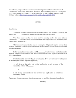

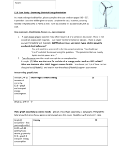


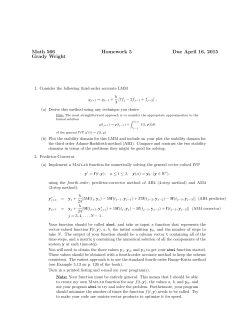

© Copyright 2026