Politecnico di Torino
Porto Institutional Repository
[Doctoral thesis] Studies on monolithic active pixel sensors for the Inner
Tracking System upgrade of ALICE experiment
Original Citation:
Aimo Ilaria (2015). Studies on monolithic active pixel sensors for the Inner Tracking System upgrade
of ALICE experiment. PhD thesis
Availability:
This version is available at : http://porto.polito.it/2596378/ since: March 2015
Published version:
DOI:10.6092/polito/porto/2596378
Terms of use:
This article is made available under terms and conditions applicable to Open Access Policy Article ("Creative Commons: Attribution 3.0") , as described at http://porto.polito.it/terms_and_
conditions.html
Porto, the institutional repository of the Politecnico di Torino, is provided by the University Library
and the IT-Services. The aim is to enable open access to all the world. Please share with us how
this access benefits you. Your story matters.
(Article begins on next page)
6
DEVELOPEMENT OF A
TESTBEAM TELESCOPE BASED
ON MAPS
Contents
6.1
6.2
6.3
The telescope setup
81
6.1.1
June Setup
6.1.2
September Setup
6.1.3
MIMOSA28
83
6.1.4
MIMOSA18
83
6.1.5
MIMOSA22 ThrB
6.1.6
Data acquisition system
81
Analysis procedure
82
84
84
85
6.2.1
Alignment
6.2.2
Tracking
86
Analysis Results
89
85
6.3.1
Efficiency
6.3.2
Spatial Resolution
6.3.3
Fake Hit Rate
89
91
96
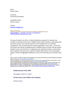
(a) Telescope overview
(b) Close up of the 7 layers composing the telescope
Figure 46: Telescope overview at the Beam Test Facility (INFN Laboratori
Nazionali di Frascati)
A telescope composed of 4 planes of MIMOSA28 and 2 planes of
MIMOSA18 chips (monolithic pixel sensors both developed in the
0.35 µm AMS process) is under development at the DAΦNE Beam
Test Facility (BTF) at the INFN Laboratori Nazionali di Frascati (LNF)
80
6.1 the telescope setup
81
in Italy. The telescope has been recently used to test a MIMOSA22ThrB
chip (a monolithic pixel sensor built in the 0.18 µm TowerJazz process)
and it is foreseen to perform tests on the full scale chips for the ALICE
ITS upgrade in the early 2015. Fig. 46 shows the setup used during
the testbeams of June and September 2014.
6.1
the telescope setup
The telescope has been used so far in two testbeams at the BTF
facility in Frascati (RM), the first in June and the second in September
2014.
In both the occasions the Device Under Test (DUT) was a MIMOSA22ThrB but the telescope setup was slightly different.
6.1.1 June Setup
2 × M28
2 × M28
DUT
Pl.4
Pl.7
September
6 mm
Pl.6
Pl.3
Pl.2
Pl.1
Beam
Pl.5
2 × M18
54 mm
1.6 mm 12 mm
90 mm
6 mm
September: 62mm
Figure 47: Telescope overview during testbeams (not to scale). In black the
original setup used in June 2014, in blue the modifications made
to the setup in September. In red the identification number of
each plane is shown.
Fig. 47 shows a scheme of the telescope setup during the data taking. The incoming beam first hits the first pair of MIMOSA28 chips,
placed at a distance of ≈ 0.6 cm from each other. The DUT (MIMOSA22ThrB) is placed at a distance of ≈ 9 cm from the second
plane of MIMOSA28. A pair of MIMOSA18 is positioned very close
(1.2 cm) to the DUT; the two sensors of MIMOSA18 are bonded on
6.1 the telescope setup
the two opposite sides of the same board and are therefore very close
to each other (1.6 mm), to minimize the effect of the lever arm for
multiple scattering. A second pair of MIMOSA28 is placed downstream, whose first plane is placed at 5.4 cm from the MIMOSA18
doublet. Moreover between the first couple of MIMOSA28 and DUT
a plane of MIMOSA22ThrA was placed. It was planned to be used as
a further DUT but it was never connected with the DAQ. Anyway its
presence must be taken into account for the multiple scattering effect.
During this testbeam we were not main users: the beam was not
centred on the telescope and the particle rate was limited to a few
particles/cm2 per frame. As a consequence, the number of runs with
very high statistics was limited.
6.1.2 September Setup
During the September testbeam the plane of MIMOSA22ThrA was
removed from the telescope and the two first planes of MIMOSA28
were positioned closer to the DUT (at a distance of ≈ 6.2 cm). From
the DUT going downstream no variations were made in the plane positions with respect to the June setup, nevertheless the seventh plane
of the telescope (MIMOSA28) had some technical issues and was not
included in the DAQ. Thus only 5 out of 6 planes of the telescope
were available.
Profiting of being main users at the BTF, during this shift it was
possible to center the telescope respect to the beam and to increase
the particle rate up to ≈ 100 particles/cm2 per frame.
Fig. 48 shows the beam profile as seen on the second MIMOSA28
plane: it is clearly visible the different position of the telescope with
respect to the beam.
(a) June 2014
(b) September 2014
Figure 48: Profile of the beam as seen on one of the plane of MIMOSA28 in
June (Fig. 48a) and in September (Fig. 48b)
82
6.1 the telescope setup
(a) MIMOSA28
(b) MIMOSA18
Figure 49: Close up of the MAPS sensors composing the telescope
6.1.3 MIMOSA28
The MIMOSA28 (see Fig. 49a) sensor (M28, ULTIMATE) is the final sensor developed for the upgrade of the inner layer of the vertex
detector of the STAR experiment at RHIC. This chip has been fabricated in the 0.35 µm AMS opto process. It is a matrix of 928 (rows)
× 960 (columns) digital pixels of 20.7 µm pitch, for a total chip size
of 20.22 × 22.71 mm2 . The sensor has an epitaxial layer thickness
of 15 µm on a High Resistivity substrate (400 Ωcm) and has been
thinned down to 50 µm to reduce the material budget. Pixel columns
are readout in parallel, row by row; the readout time is 185.6 µs.
Each pixel includes an amplification and Correlated Double Sampling (CDS) and each end of columns is equipped with a discriminator. The threshold of the discriminator is programmable by JTAG
slow control. After analog to digital conversion, the digital signals
pass through the zero suppression block: digital signals are processed
in parallel on 15 banks, then arranged and stored in a memory row
by row.
6.1.4 MIMOSA18
The Mimosa-18 sensor (M18) [68] has been fabricated in the 0.35 µm
AMS opto process and is a composed of 4 matrices of 256 × 256 analog
pixels with a pitch of 10 µm. Therefore a single sensor consists of an
array of 512 × 512 pixels, providing a total area of 5 × 5 mm2 .
The sensor is fabricated using a standard 14 µm thick epitaxial layer
and has been thinned down to 50 µm. A simple read out architecture
is used: it consists of a 2-transistor pixel cell (half of a source follower
plus a readout selection switch) connected to the charge collecting
Nwell diode, continuously biased by another diode (forward biased)
implemented inside sensing Nwell. The size of the sensing Nwell
diode is of 4.4 µm × 3.4 µm. The signal information from each pixel is
serialized by a circuit (one per sub-array), which can withstand up to
83
6.1 the telescope setup
a 25 MHz readout clock frequency. However, all the results presented
in this work were obtained with a 20 MHz clock, which provides a
full frame readout time of ∼ 3 ms.
In this architecture, the frame readout time is equal to the signal
integration window. Information from two consecutive frames was
read out, one frame before and one frame after each trigger. Correlated double sampling (CDS) method was used for hit reconstruction.
6.1.5 MIMOSA22 ThrB
The MIMOSA22-ThrB (M22-ThrB) [69] has been designed in TowerJazz 0.18 µm process on a high resistivity epitaxial layer. The sensor
is composed of a matrix of 64 × 64 elongated pixels, with a pixel
size of 33µm × 22µm. Its architecture is based on the MIMOSA22
which is a fast binary readout MAPS, with an integration time of
6.4 µs. At the bottom of the matrix there are 56 columns composed
of two discriminators for double row readout and 8 columns formed
of 2 output buffers for double row readout. The matrix is controlled
by internal fully programmable digital sequencer and integrates each
one output multiplexers for 16 binary outputs. The chip is driven by
a 100 MHz clock. The setup with programmable registers is accessed
via an embedded slow control JTAG interface.
6.1.6 Data acquisition system
The Data Acquisition system (DAQ) is based on the VME bus standard. The whole system consists of four V1495 (General Purpose
VME board, equipped with a EP1C20 Altera Cyclone FPGA) modules
by Caen, one ADC SIS3300 and one ADC SIS3301 boards by Struck,
one V895 (16 channel leading edge discriminator) by Caen and one
V2718 VME controller optical bridge by Caen. The 8 analog signals
from the M18 are sampled by the 8 differential inputs of the SIS3301
module. The SIS3300 has 8 single-ended analog inputs, which are
used to acquire the data from the beamline calorimeter and the beam
signal from the BTF. This BTF signal has a repetition rate of 25 ns
(the pulse duration is a few ns) and is used as trigger for the whole
system. The trigger signal is sent to one input of the V895 board (low
threshold discriminator), which in its turn sends its output pattern to
one of the V1495, which also acts as Trigger Supervisor. The Trigger
Supervisor sends the trigger signals to all the other V1495 modules; it
also manages the BUSY signal: at each trigger, the Trigger Supervisor
stops and, before accepting more trigger signals, it waits to be reset
by the acquisition software. The Trigger Supervisor also produces a
common clock at 80 MHz which is distributed to all the four V1495.
One of the four V1495 is then used to generate the control signals
for the SIS3300 and SIS3301, which are working at a clock frequency
84
6.2 analysis procedure
of 20 MHz (the same frequency as the M18); the other V1495 modules are used to generate all the digital control signals for the 7 chips,
to readout and store in some FIFOs internal to the FPGA the digital
outputs from the four M28 and the two M18. The initialization procedures for the four M28 and the two M18 are managed by a software
which reads out the respectively ASCII Configuration Files and sends
the proper signals to the sensors through the V1495, which act as a
parallel port.
6.2
analysis procedure
An electron beam with an energy of 500 MeV has been used. Data
were collected for different threshold values in Signal to Noise ratio
(SNR) applied to the DUT in order to test the dependence of the
efficiency on the SNR cut.
Data were analysed using TAF [70], which stands for TAPI Analysis Framework, the package created and managed by the PICSEL
group at IPHC (Strasbourg, France) to characterize CMOS pixel and
strip sensors from data acquired with various sources (X-rays, β-rays,
laser) or with particle beams.
The cluster position is reconstructed as centre of gravity of the pixels belonging to the cluster.
6.2.1 Alignment
Fig. 50 shows the correlation plots in horizontal and vertical direction between the two planes of MIMOSA18. The plots are built plotting the horizontal (vertical) hit position on one plane as a function
of all the other horizontal (vertical) hit positions of the same event on
the other plane. If a particle has crossed the telescope the hit position
on the two planes are necessarly correlated.This leads to a region in
the scatter plot where a correlation between the hit positions in the
two planes is clearly visible
The different correlation directions in the scatter plot along the two
coordinates are due to the mutual position of the two MIMOSA18
sensors; indeed, they are mounted on the two side of the same board
rotated of 180◦ one respect to the other.
The correlations between hits of different planes mean that particles have crossed the telescope, but to properly track through all the
planes it is necessary to apply some corrections to the measured plane
positions in order to take into account their real mutual position.
The 6 planes of the telescope were first aligned plane by plane
(alignment is not done globally), starting from one plane chosen as
reference (called seed plane ) with an iterative semi-automatic procedure. The track starts with a single hit in the reference plane and
85
6.2 analysis procedure
with zero slope. Then, the track seed extrapolation to the next plane
defines the centre of a circular search area. If there are hits on this
plane within the search area, the nearest one to the centre is associated to the track. The track parameters are then recomputed and the
iteration goes on with the next plane. Once all the planes have been
scanned, the track is tested against selection cuts.
Due to the different conditions during the two testbeams, align
procedure has been performed in different way with the June and
September data.
In June the alignment strategy started with the definition of plane 6
as the reference plane. Then plane 7 was aligned with respect to plane
6. Using tracks passing through plane 6 and 7, plane 4 and 5 were
then aligned. Finally tracking with plane 4, 5, 6 and 7 the alignment
has been performed on plane 1 and 2. DUT was then aligned with
respect to the telescope.
In September it was not possible to use the same procedure since
plane 7 was not included in the DAQ. Thus in the alignment procedure plane 2 was considered as the reference plane, then plane 1 was
aligned with respect to that. Profiting of the high statistics, the DUT
was included in the procedure and aligned with respect to plane 1
and 2. Then planes 4 and 5 were aligned using as a reference the first
three planes and, eventually, plane 6 was aligned with respect to the
other five planes.
µm
Correlation rows Pl4-Pl5
µm
Correlation columns Pl4-Pl5
120
2000
180
2000
160
140
100
1000
1000
120
80
100
0
0
60
-1000
40
80
60
-1000
40
20
-2000
-2000
-2000
-1000
0
1000
2000
µm
0
20
-2000
-1000
0
1000
2000
µm
0
Figure 50: Correlation plots between hits on Plane 4 and 5 (M18) of the
Telescope (September setup). Left panel: correlation of hits along
column direction. Right panel: correlations of hits along rows
direction.
6.2.2 Tracking
After alignment, tracks reconstruction has been performed. As for
the tracking strategy, a hit in at least 4 out of 6 planes (4 out of 5 for
September data) is required to make a track. Usually a distance lower
than 400 µm is required for a hit-track association. The track fitting
model is a straight line (parameters obtained from a least square fit):
no multiple scattering is considered. The DUT is, of course, excluded
from the tracking procedure.
86
6.2 analysis procedure
Fig. 51 shows the statistics on the tracking results. The left panel
(Fig. 51a) represents the distribution of the fraction of times (in percentage) each plane has been used to fit a track while the right one
shows the distribution of the number of hits on different planes used
to fit a track. It is possible to notice that in June nearly 100% of the
tracks has been obtained with 4 planes, the majority using plane number 1,2,6 and 7 (i.e. the four plane of M28, composing the telescope).
This is due to the fact that having 4 planes of M28, which have a
sensitive area ≈ 16 times greater than the M18, and requiring at least
4 points to make a track, excludes from the tracking algorithm the
M18 sensors in most of the cases. In the analysis of September data,
instead, the majority of tracks has been obtained using 5 planes, all
the telescope planes available. The reason is that in this case requiring 4 hits to make a track necessarily includes one of the M18 planes
in the fit procedure and, since they are so close one to the other, almost always it is possible to find a hit associated to the track within
the searching region on the other M18 plane (much less affected by
multiple scattering effect).
Track hit multiplicity
September
June
102
% of Reconstructed tracks
% of Reconstructed tracks
ID of Planes used to Fit Track
September
June
102
10
1
0
1
2
3
4
5
6
7
Plane
(a) Distribution of the fraction of times
each plane has been used to fit a
track.
2.5
3
3.5
4
4.5
5
5.5
6
6.5
7
7.5
Plane
(b) Distribution of the number of planes
used to fit a track.
Figure 51: Statistics on the planes used (Fig. 51a) and on the number of
hits on different planes (Fig. 51b) used to fit a track. Blue solid
distributions refer to June data, while red dotted ones refer to
September data.
Fig. 52 shows the residuals distributions for the different telescope
planes in the vertical coordinate after the tracking procedure. They
are obtained as the distribution of the hit-track distance in the vertical
direction. Similar results have been obtained in the other coordinate.
Plots are normalized to the number of reconstructed tracks. This plots
can be used to check the alignment precision reached. The residuals
distribution should have a gaussian shape, centred at 0. Their width
depends on the resolution of sensor itself, the global resolution of the
telescope and on the multiple scattering effect.
From the distributions, the different conditions and strategy used
to align the telescope in the two testbeams are evident.
87
6.2 analysis procedure
Hit-track vertical residual, plane 2
September
June
0.035
Fraction of tracks
Fraction of tracks
Hit-track vertical residual, plane 1
0.04
September
June
0.04
0.035
0.03
0.03
0.025
0.025
0.02
0.02
0.015
0.015
0.01
0.01
0.005
0
-50
0.005
-40
-30
-20
-10
0
10
20
30
40
0
-50
50
µm
-40
-30
(a) Plane 1 (M28)
Fraction of tracks
Fraction of tracks
June
0.05
0.03
0.02
0.02
0.01
0.01
0
10
20
30
40
0
-50
50
µm
-40
-30
(c) Plane 4 (M18)
40
50
µm
-20
-10
0
10
20
30
40
50
µm
(d) Plane 5 (M18)
Hit-track vertical residual, plane 7
0.024
September
0.022
June
0.02
0.018
Fraction of tracks
Hit-track vertical residual, plane 6
Fraction of tracks
30
June
0.04
-10
20
September
0.03
-20
10
0.05
0.04
-30
0
Hit-track vertical residual, plane 5
September
-40
-10
(b) Plane 2 (M28)
Hit-track vertical residual, plane 4
0
-50
-20
0.025
June
0.02
0.016
0.015
0.014
0.012
0.01
0.01
0.008
0.006
0.005
0.004
0.002
0
-50
-40
-30
-20
-10
0
10
20
(e) Plane 6 (M28)
30
40
50
µm
0
-50
-40
-30
-20
-10
0
10
20
30
40
50
µm
(f) Plane 7 (M28)
Figure 52: Telescope planes residual (hit-track distance) distributions in vertical direction after alignment procedure. Distributions are normalized to the total number of reconstructed tracks. Blue solid
distributions refer to June data, while red dotted ones refer to
September data.
As far as June is concerned, the alignment strategy started from
plane 6 and the first couple of planes that were aligned was 6 and
7, while the last was 1 and 2. For this reason it is possible to notice
that the residuals distributions of the last two planes of the telescope
show a narrow peak 0-centred (with a FWHM of ≈ 10 µm) while the
residuals of the first two planes have a broad distribution which is not
centred at 0 but rather at ≈ 15 µm for plane 1 and at ≈ −15 µm for
plane 2. This means that they are not perfectly aligned with respect
to the others planes and that the multiple scattering effect has an
important effect on the tracking precision.
88
6.3 analysis results
The different strategy applied in September led to an opposite situation in the residuals distribution, in this case in fact the narrow
distributions are on plane 1 and 2 while, although centred at 0, plane
6 presents a broad peak. This means that the higher statistics and the
better position with respect to the beam in this occasion improved the
alignment capability of the telescope but the multiple scattering still
has an important effect.
In the case of plane 4 and 5, instead, the small pitch of the pixel,
the analogue readout and their close mutual position allow to have
a distance of the tracks associated to a hit on the DUT distribution
whose width is comparable for the two testbeams.
6.3
analysis results
6.3.1 Efficiency
The detection efficiency of the DUT has been measured for different
values of the discriminators threshold set on the DUT quoted in units
of noise (in the following noted as SNR threshold applied, quoted in
terms of number of σ). Efficiency has been evaluated as the ratio
between the number of tracks associated to a hit in the DUT, within a
certain distance, and the total number of tracks passing through the
sensitive region of DUT. As a further selection criteria a cut on χ2 has
been applied. Only tracks with χ2 < 45 have been accepted.
Fig. 53 shows the map of the hits on the DUT associated to a track
(left panels) and the map of the track impact positions on the DUT
which could not be associated with any hit on the DUT (right panels).
Two runs with the same SNR threshold applied on the DUT (9 σ) are
compared: in the top panels plots refer to June data, in the bottom to
September ones.
From the plots it is evident the different statistics available in the
two runs (see Tab. 9). However in both the testbeams the whole area
of the DUT was illuminated by the sensors and no zone of inhomogeneity in the rejection of the tracks are present, meaning that the
behaviour of the DUT is the same over the whole sensitive area.
Fig. 54 shows, for the same runs previously discussed, the distribution of the track-hit distance of the tracks associated to an hit on the
DUT. The majority of the hits has a distance to the associated track
below 100 µm. In this case the maximum distance allowed to match
hit with tracks was set to 500 µm in order to take into account the
possible great effect of multiple scattering for electrons of 500 MeV.
The cut seems reasonable since it seems to cut only the very tail of
the distributions.
Fig. 55 shows the efficiency as a function of the SNR threshold applied to the discriminators of the DUT. For the June data the calcula-
89
6.3 analysis results
UNMATCHED track map
[µm]
3
[µm]
MATCHED hit map
1000
2.5
500
2
1
800
0.9
600
0.8
400
0.7
0.6
200
1.5
0
0.5
0
0.4
1
-500
-200
0.3
-400
0.2
0.5
-1000
0.1
-600
-600
-400
-200
0
200
400
600
0
800
[µm]
-300
-200
-100
(a) June
0
100
200
300
400
0
[µm]
(b) June
UNMATCHED track map
50
2
[µm]
[µm]
MATCHED hit map
1.8
1000
1000
1.6
40
1.4
500
500
1.2
30
1
0
0
0.8
20
-500
0.6
-500
0.4
10
-1000
-1000
-600
-400
-200
0
200
400
600
0.2
0
800
[µm]
-600
-400
-200
(c) September
0
200
400
600
0
800
[µm]
(d) September
Figure 53: Left panels: maps of hits (Cluster Centre of Gravity) on the DUT
matched to a track crossing the DUT. Right panels: maps of track
impact positions on the DUT which could not be associated to
any tracks in the DUT. Top plots refer to June data, bottom to
September ones. Both in June and September the SNR threshold
on the DUT was 9σ and the maximum distance to associate hit
to tracks was 500 µm.
Track-Hit Distance, MATCHED hits
Track-Hit Distance, MATCHED hits
DuvCG
Entries
102
534
Mean
18.69
RMS
21.07
103
DuvCG
Entries
16654
Mean
20.75
RMS
45.24
102
10
10
1
1
0
50
100
150
(a) June
200
250
(µm)
0
50
100
150
200
250
300
350
400
(µm)
(b) September
Figure 54: Distribution of the track-hit distance of hits matched to a track
on the DUT in a run where the SNR threshold on the DUT was
9σ.
tion has been made considering both the whole area of the DUT and
the area excluding a 2-pixels external crown, in order to exclude uncompleted clusters. The maximum distance to associate hit to tracks
on DUT was 500 µm. In September instead two different cuts on the
90
6.3 analysis results
maximum distance have been used: 400 µm and 500 µm; in both cases
the 2-pixels external crown has been removed from the region of interest for the hits on the DUT. The numerical values of the efficiencies
shown in Fig. 55 are reported in Tab. 9. Errors on the efficiency have
been evaluated as the variance of a binomial distribution.
It is possible to notice that:
• Excluding the two pixel external crowns has a marginal effect,
efficiency evaluated with or without this region are compatible
within the error bars. It has been chosen to exclude the external
region in the second testbeam in order to avoid cut clusters.
• The different maximum distances affect the efficiency evaluation especially at higher SNR threshold.
• Both in June and in September data efficiency is close to 99% up
to SNR threshold of 9σ and then it drops, meaning that for cuts
> 9 σ we are starting to lose signal.
• Even though the maximum distance allowed to associate hit to
track was 500 µm, actually, the hit-to-track distributions (Fig. 54)
show that the association is mostly made within 100 µm. With
a fake hit rate at this SNR of 3 · 10−4 (see Sec. 6.3.3) the possible
contribution from noisy pixels within the searching region is
negligible.
• June and September evaluations of the efficiencies for runs with
the same thresholds are compatible within the errors.
6.3.2 Spatial Resolution
Spatial resolution has been evaluated with the June and September
data using a 9σ SNR threshold.
The spatial resolution of the DUT has been estimated from the hits
residual distributions. These distributions are obtained with the difference between the impact position of the particle extrapolated from
the track direction and the position of the hit associated to that track
on the DUT. The hit position on the DUT is evaluated as the centre of
gravity of the cluster distribution.
Fig. 56 shows, as example, the residual distributions on the DUT
in both vertical and horizontal directions for the September dataset.
Similar results have been obtained in June. The distributions are gaussian shaped and centred at 0. Starting from the width of the residuals
distribution (evaluated as the standard deviation of a gaussian fit) it
is possible to give an estimation of the spacial resolution of the DUT.
The width of the residual distribution, however, is not only affected
by the DUT resolution but also by the resolution of the telescope itself.
91
309 ± 5%
1778 ± 2%
631 ± 4%
829 ± 3%
3677 ± 1%
Associated
tracks
311 ± 5%
1790 ± 2%
640 ± 4%
864 ± 3%
3917 ± 1%
Tot. tracks
through DUT
99.2 ± 0.5
99.3 ± 0.2
99.1 ± 0.4
96.0 ± 0.7
93.9 ± 0.4
Efficiency
[%]
Tot. tracks
through DUT
47257 ± 0.5%
160223 ± 0.2%
79332 ± 0.3%
172601 ± 0.2%
102962 ± 0.3%
84491 ± 0.3%
9059 ± 1%
8982 ± 1%
25058 ± 0.6%
41771 ± 0.5%
Associated
tracks
47228 ± 0.5%
159754 ± 0.2%
78763 ± 0.4%
169884 ± 0.2%
99508 ± 0.3%
79226 ± 0.4%
8094 ± 1%
7724 ± 1%
21114 ± 0.7%
34135 ± 0.5%
dhit−tr < 400 µm
99.96 ± 0.02
99.71 ± 0.01
99.28 ± 0.03
98.42 ± 0.03
96.64 ± 0.06
93.77 ± 0.09
89.3 ± 0.3
86.0 ± 0.4
84.4 ± 0.2
81.7 ± 0.2
Efficiency
[%]
42247 ± 0.5%
159939 ± 0.3%
78910 ± 0.4%
170405 ± 0.2%
99848 ± 0.3%
11771 ± 0.4%
8164 ± 1%
7810 ± 1%
21595 ± 0.7%
79699 ± 0.5%
Associated
tracks
September
47257 ± 0.5%
160223 ± 0.2%
79332 ± 0.4%
172601 ± 0.2%
102962 ± 0.3%
12485 ± 0.3%
9059 ± 1%
8982 ± 1%
25058 ± 0.6%
84491 ± 0.3%
Tot. tracks
through DUT
dhit−tr < 500 µm
99.900 ± 0.008
99.82 ± 0.01
99.47 ± 0.03
98.72 ± 0.03
96.97 ± 0.05
94.32 ± 0.08
90.1 ± 0.3
86.9 ± 0.3
86.2 ± 0.2
84.3 ± 0.2
Efficiency
[%]
Table 9: Summary of the efficiency values found for different SNR used to acquire the DUT data (σ) and number of tracks used to evaluate the
efficiencies. In bold font values obtained in the same conditions in June and September.
6
7
8
9
10
11
13
14
15
16
σ
June
dhit−tr < 500 µm
6.3 analysis results
92
6.3 analysis results
(a) June dataset. Blue points are obtained excluding
the two external pixels crown of the DUT matrix,
red ones considering instead the whole DUT matrix.
Maximum distance to associate hits to tracks on the
DUT is 500 µm
(b) September dataset. Green circles are obtained considering as maximum distance to associate hits to
tracks on the DUT 500 µm, blue triangles using instead 400 µm. In both cases the external two pixels
crown of the DUT has been excluded from the searching region.
Figure 55: DUT Efficiency as a function of the SNR cut used to acquire the
DUT data
June
September
Horizontal
[µm]
Vertical
[µm]
9.1 ± 0.5
8.65 ± 0.02
10.7 ± 0.4
10.59 ± 0.02
Table 10: DUT Residual width (σ of the gaussian fit of distributions shown
in Fig. 56) in a run with 9σ threshold
Namely the residual distribution is a convolution of two gaussians
with different width: one including the contribution of the telescope
resolution and the multiple scattering effect (with a standard devi-
93
6.3 analysis results
DUT Residuals - Horizontal direction
DUT Residuals - Vertical direction
8000
1.229e+04 / 530
7273 ± 26.2
Constant
-0.1259 ± 0.0218
Mean
7000
8.647 ± 0.022
Sigma
# of Reconstructed tracks
# of Reconstructed tracks
7000
χ2 / ndf
χ2 / ndf
Constant
6000
Mean
Sigma
7689 / 526
6106 ± 20.7
-1 ± 0.0
10.59 ± 0.02
5000
6000
5000
4000
4000
3000
3000
2000
2000
1000
1000
0
-200
-100
0
100
200
Track-Hit distance [µ m]
(a) DUT residuals distribution, columns
direction
0
-200
-100
0
100
200
Track-Hit distance [µ m]
(b) DUT residuals distribution, rows direction
Figure 56: DUT residuals distributions along columns (Fig. 56a) and rows
(Fig. 56b) directions. The hit position on the DUT is reconstructed as the center of gravity of the cluster. September setup
configuration. SNR cut on DUT data was 9 σ
σ of DUT Residuals distribution
hit-track distance [µm]
11.5
September
June
11
10.5
10
9.5
9
8.5
8
horizontal
vertical
direction
Figure 57: Comparision of the residual distribution width (evaluate obtained in June and in September
ation noted as resTEL ) and one due to the DUT resolution (with a
different width resDUT ). For this reason, the σ of the residual distribution can be expressed like shown in Eq 21.
q
σ = res2tel + res2DUT
(21)
Fig. 57 shows a comparision of the σ (standard deviation of the
gaussian fit) of the residuals distribution for both June and September data. It is possible to notice that the two results obtained are compatible within the errors, which, in this case, are expressing only the
94
6.3 analysis results
statistical uncertainty of the interpolation. However this uncertainty
for the September data is much more smaller thanks to the higher
statistics available. The same results are summarized also in Tab. 10.
The differences between the horizontal and vertical directions can be
explained with the different pitch of the pixels in the two directions
(22 µm in the horizontal direction and 33µm in the vertical one).
A first estimation for the telescope resolution has been obtained
with a Toy Monte-Carlo included in the TAF software package, implementing the geometry used for the testbeam, obtaining the same
results for the two configurations:
restel = (8.0 ± 0.5) µm
(22)
This led to the estimated DUT spatial resolution noted in tab. 11
DUT resolution
Horizontal Vertical
[µm]
[µm]
June
September
4.3 ± 0.7
3.3 ± 0.5
7.1 ± 0.6
6.9 ± 0.6
Table 11: DUT Resolution estimation. The SNR threshold set on DUT discriminators was 9σ. Only statistical uncertainty are quoted.
The results obtained are generally in line with the ITS upgrade
requirement, however a few approximations were done:
• As far as June setup is concerned, the plane of M22ThrA, which
should be considered as a passive plane, was not included in the
simulation. The Toy Monte-Carlo indeed has not this possibility
currently implemented.
• The uncertainties here quoted only include the statistical error
deriving from the fit and the simulation. They do not take into
account a possible systematic effect due to inefficiencies in the
alignment procedure. In particular the TAF alignment procedure has been developed for much higher energy of the incoming beam where multiple scattering has a smaller effect.
To overcome this limitations some GEANT3 simulations are currently ongoing to better estimate the telescope resolution. The idea
of this simulations is to use GEANT3 to implement the geometry of
the telescope and to transport particles through the telescope and
then use directly TAF to reconstruct the tracks. In this way the DUT
residuals distribution obtained are taking into account only the contribution of the multiple scattering since the impact position on the
DUT is known in the simulation.
95
6.3 analysis results
Average=1.225 ﬁred pixels per ev.
Average fake
hit rate = 3 10-4
Figure 58: Top left panel: raw hit distribution in a run of 1000 events without beam with a SNR threshold of 9σ . Top right panel: distribution of the number of hit pixels in each event during the run.
Average number of hit pixels corresponding to 1.225 is indicated
in the plot . Bottom left panel: fake hit rate ditribution obtained
as the frequency of hit per pixel per event. Bottom right panel:
distribution of the fraction of pixels below a certain fake hit rate
value.
Another option under investigation is to directly measure the telescope resolution by keeping the very same geometry for the telescope
planes, and replacing the DUT with a high resolution device. The
M18 would be a proper candidate: it is an analog detector with a
very small pitch (10 µm), which might provide a resolution close to
1 µm. We plan to carry out this measurement in one of the next test
beams.
6.3.3 Fake Hit Rate
Fake hit rate has been evaluated in events with no beam, for different thresholds set on the DUT discriminators.
Fig. 58 shows the results obtained for SNR threshold on DUT equal
to 9σ. Top left plot is showing the hit map on the DUT over 1000
events, the top right one presents the distribution of the number of
fired pixels per events, the average of the distribution is also plotted
and, in this case, was equal to 1.225 fired pixels per event. Fake hit
rate is evaluated dividing the number of fired pixels per events by the
total number of pixels in the matrix and the number of events. The
left bottom plot of Fig. 58 shows the fake hit rate distribution. The
average fake hit rate per pixel is 3 10−4 . The right bottom plot shows
the fraction of pixels in the sensor which have a fake hit rate lower
than a certain value. It is possible to see that the 99% of pixels in the
DUT has a fake hit rate below 10−3 .
96
6.3 analysis results
Figure 59: Fake hit rate on the DUT as a function of the SNR cut applied on
the DUT data taking
Calculation has been repeated for different SNR thresholds and the
average Fake Hit Pixel as a function of the threshold applied is shown
in Fig. 59.
It is possible to notice that the fake hit rate decreases up to SNRthr =
13 σ and then remains stable to a value ≈ 10−5 /pixel.
Although this result is in line with the requirements for the upgrade it has to be mentioned that the prototype used as DUT has a
small number of pixels and it is not corrected for the known effect
of “Random Telegraph Signal” noise (RTS). The RTS noise originates
from the presence of defects in the oxide layer of a MOS transistor.
It depends on different variables including temperature, gate voltage
of the transistor and the oxide thickness. It manifests itself as discrete changes of individual pixel output between two (or more) levels.
While the amplitude of this signal is well defined, its period is random and may reach minutes. The amplitude of the RTS is sufficient
to exceed the pre-set threshold of the detector and may therefore generate fake hits. The Fake Rate here described is dominated by these
two effects.
97
7
CONCLUSION
Recent developments in the field of Monolithic Active Pixel Sensor (MAPS) technology have opened a window of possibilities for
their use as vertexing and tracking detectors in particle physics experiments. ALICE has an elaborate upgrade programme based on
the upgrade of the LHC in 2018-19 during the second Long Shutdown (LS2).
ALICE has already demonstrated very good capabilities for the
study of heavy ion collisions at high energy in its first three years
of operation. But there are particular measurements, like high precision measurements of rare probes over a wide range of momenta,
which would require high statistics and are not satisfactory or even
possible with the present experimental setup. These measurements
would help to achieve the long term physics goals of ALICE and
would go a long way forward in understanding and characterizing
the Quark Gluon Plasma (QGP) state of matter. The LHC upgrade
features which primarily motivated the ALICE upgrade programme
are Pb–Pb collisions with a high interaction rate of up to 50 kHz, corresponding to an instantaneous luminosity L = 6 × 1027 cm−2 s−1 and,
the installation of a narrower beam pipe.
Accordingly, ALICE would require detector upgrades to cope with
the new scenario.In particular the upgraded ALICE apparatus should
improve tracking and vertexing capabilities, radiation hardness and
should allow readout of all interactions to accumulate enough statistics for the extended physics programme. The objective is to accumulate 10 nb−1 of Pb-Pb collisions, recording about 1011 interactions.
Within this upgrade strategy, the Inner Tracking System (ITS) upgrade forms an important cornerstone, providing improved vertexing
and readout capabilities. The new ITS will have a barrel geometry
consisting of seven layers of Monolithic Active Pixel Sensors (MAPS)
with high granularity. The geometry is optimized for high efficiency,
both in standalone tracking and ITS-TPC combined tracking.
TowerJazz 0.18 µm technology has been selected for designing the
pixels for ITS upgrade. This technology provides attractive features
like, for example, the option to implement a deep p-well allowing the
implementation of a full CMOS process in the pixel.
Several prototypes have been designed to investigate and validate
the different design strategies and the different components of the
pixel detector using this technology. The design R&D is being carried out at CNU (Wuhan, China), CERN, INFN (Italy), NIKHEF (The
Netherlands), Yonsei (South Korea) and IPHC Strassbourg.
98
conclusion
The ongoing research and development on these pixels investigates
different design strategies and would converge towards at the beginning of 2015.
MIMOSA32 and MIMOSA32Ter, developed at IPHC Strassbourg,
were one of the first prototypes designed with the TowerJazz technology for the upgrade program. The motivation was to validate
the technology in terms of charge collection and radiation tolerance.
These prototypes also implemented deep p-well structures (without
implementing a full CMOS in the pixel circuit) to qualify its usage for
future prototypes using a full CMOS process.
This thesis studied the results of tests and characterization of pixel
structures of these prototypes and concluded that the technology provided the basic requirements of charge collection and radiation tolerance. It also concluded that the addition of a deep p-well maintains
satisfactory performance even after irradiation. This marks a starting
point for future prototypes where the deep p-well could be implemented in a full CMOS process, thus allowing in-pixel sophisticated
signal processing circuits.
To study the detection efficiency and the spacial resolution of the
prototypes a telescope of sensors capable to provide external tracking is needed. In this thesis the development of a telescope of MAPS
sensor carried out at the LNF Laboratory in Frascati is presented. It
is composed of six planes of MAPS sensors: 4 planes of MIMOSA28
(0.35 µm AMS opto process, 928 rows × 960 columns, pitch of 20.7 µm,
binary readout) and two of MIMOSA18 (0.35 µmAMS opto process,
4 matrices of 256 × 256 pixels, pitch of 10 µm, analog readout). The
incoming beam first goes through two planes of MIMOSA 28, then
the DUT is placed followed by two planes of MIMOSA18 and another
couple of MIMOSA28.
This thesis shows the results obtained with this telescope using
the MIMOSA22-ThrB as DUT protoype in two testbeams carried out
in June and September 2014. Detection efficiency, spatial resolution
and fake hit rate of this prototype have been evaluated during these
two testbeams and all the measured parameters are in line with the
requirements set by the ITS upgrade.
This thesis validated the telescope setup which will be used for a
comparative study of the two full scale protoypes designed for the
ALICE upgrade: the FSBB developed in Strasbourg by IPHC PICSEL group and ALPIDEfs developed by the collaboration of CNU
(Wuhan, China), CERN, INFN (Italy), NIKHEF (The Netherlands),
Yonsei (South Korea). First test on the full scale prototypes are foreseen either for the end of 2014 or for the beginning of 2015.
99
BIBLIOGRAPHY
[1]
Edward V. Shuryak. “Quantum chromodynamics and the theory of superdense matter”. In: Physics Reports 61.2 (1980), pp. 71–
158. issn: 0370-1573. doi: http://dx.doi.org/10.1016/03701573(80 ) 90105 - 2. url: http : / / www . sciencedirect . com /
science/article/pii/0370157380901052 (cit. on p. 3).
[2]
Frithjof Karsch. “Lattice results on QCD thermodynamics”. In:
Nucl.Phys. A698 (2002), pp. 199–208. doi: 10.1016/S0375-9474(01)
01365-3. arXiv: hep-ph/0103314 [hep-ph] (cit. on p. 3).
[3]
O.W. Greenberg and C.A. Nelson. “Color models of hadrons”.
In: Physics Reports 32.2 (1977), pp. 69–121. issn: 0370-1573. doi:
http : / / dx . doi . org / 10 . 1016 / 0370 - 1573(77 ) 90035 - 7. url:
http : / / www . sciencedirect . com / science / article / pii /
0370157377900357 (cit. on p. 4).
[4]
Antonio Pich. “Aspects of quantum chromodynamics”. In: (1999).
arXiv: hep-ph/0001118 (cit. on p. 4).
[5]
M. E. Peskin and D. V. Schroeder. An Introduction to Quantum
Field Theory. Reading: Addison-Wesley, 1995 (cit. on p. 5).
[6]
Michael J. Fromerth and Johann Rafelski. “Hadronization of the
quark universe”. In: (2002). arXiv: astro - ph / 0211346 (cit. on
p. 5).
[7]
Frithjof Karsch. “Properties of the Quark Gluon Plasma: A lattice perspective”. In: Nucl. Phys. A783 (2007), pp. 13–22. doi:
10.1016/j.nuclphysa.2006.11.035. arXiv: hep- ph/0610024
(cit. on p. 6).
[8]
A. Chodos et al. “New extended model of hadrons”. In: Phys.
Rev. D 9 (12 June 1974), pp. 3471–3495. doi: 10.1103/PhysRevD.
9.3471. url: http://link.aps.org/doi/10.1103/PhysRevD.9.
3471 (cit. on p. 7).
[9]
Tetsuo Hatsuda and Teiji Kunihiro. “QCD phenomenology based
on a chiral effective Lagrangian”. In: Physics Reports 247.5-6
(1994), pp. 221–367. issn: 0370-1573. doi: 10.1016/0370-1573(94)
90022 - 1. url: http : / / www . sciencedirect . com / science /
article/pii/0370157394900221 (cit. on p. 7).
[10]
Prashant Shukla. “Glauber model for heavy ion collisions from
low energies to high energies”. In: (2001). arXiv: nucl - th /
0112039 (cit. on p. 8).
[11]
Cheuk-Yin Wong. Introduction to high-energy heavy ions collision.
World Scientific, 1994 (cit. on pp. 9, 11).
100
bibliography
[12]
ALICE Collaboration. “Centrality Dependence of the ChargedParticle Multiplicity Density at Midrapidity in Pb-Pb Collisions
√
at sNN = 2.76 TeV”. In: Phys. Rev. Lett. 106 (3 Jan. 2011),
p. 032301. doi: 10.1103/PhysRevLett.106.032301. url: http:
//link.aps.org/doi/10.1103/PhysRevLett.106.032301 (cit.
on p. 11).
[13]
ALICE Collaboration. “Charged-Particle Multiplicity Density at
√
Midrapidity in Central Pb-Pb Collisions at sNN = 2.76 TeV”.
In: Phys. Rev. Lett. 105 (25 Dec. 2010), p. 252301. doi: 10.1103/
PhysRevLett.105.252301. url: http://link.aps.org/doi/10.
1103/PhysRevLett.105.252301 (cit. on p. 11).
[14]
Serguei Chatrchyan et al. “Dependence on pseudorapidity and
centrality of charged hadron production in PbPb collisions at a
nucleon-nucleon centre-of-mass energy of 2.76 TeV”. In: JHEP
1108 (2011), p. 141. doi: 10.1007/JHEP08(2011)141. arXiv: 1107.
4800 [nucl-ex] (cit. on p. 11).
[15]
ATLAS Collaboration. “Measurement of the centrality dependence of the charged particle pseudorapidity distribution in
lead–lead collisions at with the {ATLAS} detector”. In: Physics
Letters B 710.3 (2012), pp. 363–382. issn: 0370-2693. doi: http:
/ / dx . doi . org / 10 . 1016 / j . physletb . 2012 . 02 . 045. url:
http : / / www . sciencedirect . com / science / article / pii /
S0370269312001864 (cit. on p. 11).
[16]
STAR Collaboration. “Systematic measurements of identified
particle spectra in pp, d + Au, and Au + Au collisions at the
STAR detector”. In: Phys. Rev. C 79 (3 Mar. 2009), p. 034909. doi:
10 . 1103 / PhysRevC . 79 . 034909. url: http : / / link . aps . org /
doi/10.1103/PhysRevC.79.034909 (cit. on pp. 11–13).
[17]
ALICE Collaboration. “Pion, Kaon, and Proton Production in
√
Central Pb-Pb Collisions at sNN =2.76 TeV”. In: Phys. Rev. Lett.
109 (25 Dec. 2012), p. 252301. doi: 10.1103/PhysRevLett.109.
252301. url: http://link.aps.org/doi/10.1103/PhysRevLett.
109.252301 (cit. on pp. 12, 13).
[18]
PHENIX Collaboration. “Identified charged particle spectra and
√
yields in Au + Au collisions at sNN = 200 GeV”. In: Phys.
Rev. C 69 (3 Mar. 2004), p. 034909. doi: 10.1103/PhysRevC.69.
034909. url: http://link.aps.org/doi/10.1103/PhysRevC.69.
034909 (cit. on pp. 12, 13).
[19]
Chun Shen et al. “Radial and elliptic flow in Pb + Pb collisions at energies available at the CERN Large Hadron Collider
from viscous hydrodynamics”. In: Phys. Rev. C 84 (4 Oct. 2011),
p. 044903. doi: 10 . 1103 / PhysRevC . 84 . 044903. url: http : / /
link . aps . org / doi / 10 . 1103 / PhysRevC . 84 . 044903 (cit. on
pp. 12, 13).
101
bibliography
102
[20]
Yu A Karpenko and Yu M Sinyukov. “Femtoscopic scales in
central A+A collisions at RHIC and LHC energies in a hydrokinetic model”. In: Journal of Physics G: Nuclear and Particle Physics
38.12 (2011), p. 124059. url: http : / / stacks . iop . org / 0954 3899/38/i=12/a=124059 (cit. on pp. 12, 13).
[21]
Piotr Bozek. “Hydrodynamic flow from RHIC to LHC”. In: Acta
Phys.Polon. B43 (2012), p. 689. doi: 10.5506/APhysPolB.43.689.
arXiv: 1111.4398 [nucl-th] (cit. on pp. 12, 13).
[22]
Maciej Rybczynski, Wojciech Florkowski, and Wojciech Broniowski.
“Single-freeze-out model for ultra relativistic heavy-ion colli√
sions at sNN = 2.76 TeV and the LHC proton puzzle”. In:
Phys.Rev. C85 (2012), p. 054907. doi: 10 . 1103 / PhysRevC . 85 .
054907. arXiv: 1202.5639 [nucl-th] (cit. on p. 12).
[23]
S. Voloshin and Y. Zhang. “Flow study in relativistic nuclear
collisions by Fourier expansion of Azimuthal particle distributions”. In: Z. Phys. C70 (1996), pp. 665–672. doi: 10 . 1007 /
s002880050141. arXiv: hep-ph/9407282 (cit. on p. 13).
[24]
Ulrich W. Heinz. “Concepts of heavy ion physics”. In: (2004).
These lecture notes are an expanded version of the lectures I
gave a year earlier at the 2002 European School of High-Energy
Physics in Pylos (Greece) whose Proceedings were published as
a CERN Yellow Report (CERN-2004-001, N. Ellis and R. Fleischer, eds.) The online version of these lecture notes on the
ArXiv has most graphs presented in color. PPF-SUBJECT = Experimental, Theoretical, pp. 165–238. arXiv: hep - ph / 0407360
[hep-ph] (cit. on p. 14).
[25]
STAR Collaboration. “Azimuthal anisotropy in Au+Au colli√
sions at sNN = 200 GeV”. In: Phys. Rev. C 72 (1 July 2005),
p. 014904. doi: 10 . 1103 / PhysRevC . 72 . 014904. url: http :
//link.aps.org/doi/10.1103/PhysRevC.72.014904 (cit. on
p. 14).
[26]
PHENIX Collaboration. “Elliptic Flow of Identified Hadrons in
√
Au + Au Collisions at sNN = 200 GeV”. In: Phys. Rev. Lett. 91
(18 Oct. 2003), p. 182301. doi: 10.1103/PhysRevLett.91.182301.
url: http : / / link . aps . org / doi / 10 . 1103 / PhysRevLett . 91 .
182301 (cit. on p. 14).
[27]
You Zhou. “Anisotropic flow of identified particles in Pb–Pb
√
collisions at sNN = 2.76 TeV with the ALICE detector”. In:
J.Phys.Conf.Ser. 509 (2014), p. 012029. doi: 10.1088/1742-6596/
509/1/012029. arXiv: 1309.3237 [nucl-ex] (cit. on pp. 14, 15).
[28]
Ulrich Heinz, Chun Shen, and Huichao Song. “The viscosity of
quark-gluon plasma at RHIC and the LHC”. In: AIP Conf.Proc.
1441 (2012), pp. 766–770. doi: 10.1063/1.3700674. arXiv: 1108.
5323 [nucl-th] (cit. on pp. 14, 15).
bibliography
103
[29]
Xin-Nian Wang, Miklos Gyulassy, and Michael Plümer. “LandauPomeranchuk-Migdal effect in QCD and radiative energy loss
in a quark-gluon plasma”. In: Phys. Rev. D 51 (7 Apr. 1995),
pp. 3436–3446. doi: 10 . 1103 / PhysRevD . 51 . 3436. url: http :
/ / link . aps . org / doi / 10 . 1103 / PhysRevD . 51 . 3436 (cit. on
p. 15).
[30]
Betty Abelev et al. “Centrality Dependence of Charged Particle
Production at Large Transverse Momentum in Pb–Pb Collisions
√
at sNN = 2.76 TeV”. In: Phys.Lett. B720 (2013), pp. 52–62. doi:
10.1016/j.physletb.2013.01.051. arXiv: 1208.2711 [hep-ex]
(cit. on pp. 17, 18).
[31]
STAR Collaboration. “Transverse-Momentum and Collision-Energy
Dependence of High-pT Hadron Suppression in Au + Au Collisions at Ultrarelativistic Energies”. In: Phys. Rev. Lett. 91 (17 Oct.
2003), p. 172302. doi: 10 . 1103 / PhysRevLett . 91 . 172302. url:
http://link.aps.org/doi/10.1103/PhysRevLett.91.172302
(cit. on p. 17).
[32]
PHENIX Collaboration. “High-pT charged hadron suppression
√
in Au + Au collisions at sNN = 200 GeV”. In: Phys. Rev. C 69
(3 Mar. 2004), p. 034910. doi: 10 . 1103 / PhysRevC . 69 . 034910.
url: http://link.aps.org/doi/10.1103/PhysRevC.69.034910
(cit. on p. 17).
[33]
Serguei Chatrchyan et al. “Study of high-pT charged particle
√
suppression in PbPb compared to pp collisions at sNN = 2.76
TeV”. In: Eur.Phys.J. C72 (2012), p. 1945. doi: 10 . 1140 / epjc /
s10052-012-1945-x. arXiv: 1202.2554 [nucl-ex] (cit. on pp. 17,
18).
[34]
ALICE Collaboration. “The ALICE experiment at the CERN
LHC”. In: Journal of Instrumentation 3.08 (2008), S08002. url:
%7Bhttp://stacks.iop.org/1748-0221/3/i=08/a=S08002%7D
(cit. on p. 22).
[35]
ALICE Collaboration. ALICE Offline framework, AliRoot. url: http:
//aliceinfo.cern.ch/Offline (cit. on p. 28).
[36]
R. Brun and F. Rademakers. “ROOT: An object oriented data
analysis framework”. In: Nucl.Instrum.Meth. A389 (1997), pp. 81–
86. doi: 10.1016/S0168-9002(97)00048-X (cit. on p. 28).
[37]
Rene Brun, Federico Carminati, and Simone Giani. “GEANT
Detector Description and Simulation Tool”. In: (1994) (cit. on
p. 28).
[38]
S. Agostinelli et al. “GEANT4: A Simulation toolkit”. In: Nucl.Instrum.Meth.
A506 (2003), pp. 250–303. doi: 10.1016/S0168-9002(03)013688 (cit. on p. 28).
bibliography
104
[39]
A. Fasso et al. “The FLUKA code: Present applications and
future developments”. In: eConf C0303241 (2003), MOMT004.
arXiv: physics/0306162 [physics] (cit. on p. 28).
[40]
Torbjorn Sjostrand, Stephen Mrenna, and Peter Z. Skands. “PYTHIA
6.4 Physics and Manual”. In: JHEP 0605 (2006), p. 026. doi:
10 . 1088 / 1126 - 6708 / 2006 / 05 / 026. arXiv: hep - ph / 0603175
[hep-ph] (cit. on p. 28).
[41]
G. Corcella et al. “HERWIG 6: An Event generator for hadron
emission reactions with interfering gluons (including supersymmetric processes)”. In: JHEP 0101 (2001), p. 010. doi: 10.1088/
1126-6708/2001/01/010. arXiv: hep-ph/0011363 [hep-ph] (cit.
on p. 28).
[42]
Xin-Nian Wang and Miklos Gyulassy. “hijing”. In: Phys. Rev. D
44 (11 Dec. 1991), pp. 3501–3516. doi: 10 . 1103 / PhysRevD . 44 .
3501. url: http://link.aps.org/doi/10.1103/PhysRevD.44.
3501 (cit. on p. 29).
[43]
Stefan Roesler, Ralph Engel, and Johannes Ranft. “The Monte
Carlo event generator DPMJET-III”. In: (2000), pp. 1033–1038.
arXiv: hep-ph/0012252 [hep-ph] (cit. on p. 29).
[44]
P. Saiz et al. “AliEn—ALICE environment on the {GRID}”. In:
Nuclear Instruments and Methods in Physics Research Section A: Accelerators, Spectrometers, Detectors and Associated Equipment 502.2–3
(2003). Proceedings of the {VIII} International Workshop on Advanced Computing and Analysis Techniques in Physics Research,
pp. 437–440. issn: 0168-9002. doi: http://dx.doi.org/10.1016/
S0168 - 9002(03 ) 00462 - 5. url: http : / / www . sciencedirect .
com/science/article/pii/S0168900203004625 (cit. on pp. 29,
30).
[45]
L Musa and K Safarik. Letter of Intent for the Upgrade of the ALICE Experiment. Tech. rep. CERN-LHCC-2012-012. LHCC-I-022.
Geneva: CERN, Aug. 2012 (cit. on pp. 31, 35).
[46]
ALICE Collaboration. Addendum of the Letter Of Intent for the Upgrade of the ALICE Experiment : The Muon Forward Tracker. Tech.
rep. CERN-LHCC-2013-014. LHCC-I-022-ADD-1. Final submission of the presetn LoI addendum is scheduled for September
7th. Geneva: CERN, Aug. 2013 (cit. on pp. 32, 35).
[47]
ALICE Collaboration. Technical Design Report for the Upgrade of
the ALICE Inner Tracking System. Tech. rep. CERN-LHCC-2013024. ALICE-TDR-017. Geneva: CERN, Nov. 2013 (cit. on pp. 35,
36, 38, 40).
[48]
Alessandro Grelli. “D meson nuclear modification factors in
√
Pb-Pb collisions at sNN = 2.76 TeV with the ALICE detector”.
In: Nucl.Phys. A904-905 (2013), pp. 635c–638c. doi: 10.1016/j.
bibliography
105
nuclphysa . 2013 . 02 . 096. arXiv: 1210 . 7332 [hep-ex] (cit. on
pp. 38, 40).
[49]
L Musa. Conceptual Design Report for the Upgrade of the ALICE
ITS. Tech. rep. CERN-LHCC-2012-005. LHCC-G-159. Geneva:
CERN, Mar. 2012 (cit. on pp. 39, 40).
[50]
G. Schneider. Installation of the central beryllium beam pipe in the
alice experiment. Tech. rep. EDMS: 1113439. Geneva: CERN, 2011
(cit. on p. 41).
[51]
L. Rossi et al. Pixel Detectors: From Fundamentals to Applications.
Particle Acceleration and Detection. Springer, 2006. isbn: 9783540283331.
url: http://books.google.it/books?id=AKGIXQOm0-EC (cit. on
p. 46).
[52]
L. Landau. “On the energy loss of fast particles by ionization”.
In: J.Phys.(USSR) 8 (1944), pp. 201–205 (cit. on p. 47).
[53]
P.V. Vavilov. “Ionization losses of high-energy heavy particles”.
In: (Nov. 1957) (cit. on p. 47).
[54]
Gerald R. Lynch and Orin I. Dahl. “Approximations to multiple Coulomb scattering”. In: Nuclear Instruments and Methods in
Physics Research Section B: Beam Interactions with Materials and
Atoms 58.1 (1991), pp. 6–10. issn: 0168-583X. doi: http : / / dx .
doi.org/10.1016/0168- 583X(91)95671- Y. url: http://www.
sciencedirect.com/science/article/pii/0168583X9195671Y
(cit. on p. 47).
[55]
W.R. Leo. Techniques for Nuclear and Particle Physics Experiments:
A How-to Approach. Springer, 1994. isbn: 9780387572802. url:
http : / / books . google . it / books ? id = W7vHQgAACAAJ (cit. on
pp. 48, 64).
[56]
L. Greiner et al. “A {MAPS} based vertex detector for the {STAR}
experiment at {RHIC}”. In: Nuclear Instruments and Methods in
Physics Research Section A: Accelerators, Spectrometers, Detectors
and Associated Equipment 650.1 (2011). International Workshop
on Semiconductor Pixel Detectors for Particles and Imaging
2010, pp. 68–72. issn: 0168-9002. doi: http://dx.doi.org/10.
1016/j.nima.2010.12.006. url: http://www.sciencedirect.
com/science/article/pii/S0168900210027439 (cit. on p. 50).
[57]
J.A. Ballin et al. “Monolithic Active Pixel Sensors {MAPS} in a
quadruple well technology for nearly 100% fill factor and full
CMOS pixels”. In: (2008). arXiv: 0807.2920 [physics.ins-det]
(cit. on p. 53).
[58]
A. Dorokhov et al. “High resistivity {CMOS} pixel sensors and
their application to the {STAR} {PXL} detector”. In: Nuclear Instruments and Methods in Physics Research Section A: Accelerators,
Spectrometers, Detectors and Associated Equipment 650.1 (2011). International Workshop on Semiconductor Pixel Detectors for Par-
bibliography
106
ticles and Imaging 2010, pp. 174–177. issn: 0168-9002. doi: http:
//dx.doi.org/10.1016/j.nima.2010.12.112. url: http://www.
sciencedirect.com/science/article/pii/S0168900210028925
(cit. on p. 56).
[59]
W. Snoeys et al. “Layout techniques to enhance the radiation
tolerance of standard {CMOS} technologies demonstrated on a
pixel detector readout chip”. In: Nuclear Instruments and Methods in Physics Research Section A: Accelerators, Spectrometers, Detectors and Associated Equipment 439.2–3 (2000), pp. 349–360. issn:
0168-9002. doi: http://dx.doi.org/10.1016/S0168-9002(99)
00899 - 2. url: http : / / www . sciencedirect . com / science /
article/pii/S0168900299008992 (cit. on pp. 59, 69).
[60]
S. Siddhanta et al. “The Readout System for the ALICE Zero
Degree Calorimeters”. In: Nuclear Science, IEEE Transactions on
58.4 (Aug. 2011), pp. 1759–1765. issn: 0018-9499. doi: 10.1109/
TNS.2011.2159514 (cit. on p. 63).
[61]
Lantronix Inc. XPort Description. 2013. url: https://web.archive.
org/web/20130827022033/http://www.lantronix.com/devicenetworking / embedded - device - servers / xport . html (cit. on
p. 63).
[62]
M.-M. Bé et al. Table of Radionuclides. Vol. 3. Monographie BIPM5. Pavillon de Breteuil, F-92310 Sèvres, France: Bureau International des Poids et Mesures, 2006. isbn: 92-822-2218-7. url:
http : / / www . bipm . org / utils / common / pdf / monographieRI /
Monographie_BIPM-5_Tables_Vol3.pdf (cit. on p. 64).
[63]
M Berger and M Berger. Stopping-Power and Range Tables for Electrons, Protons, and Helium Ions: Physical Reference Data. Gaithersburg, MD: NIST, 1999. url: http://www.nist.gov/pml/data/
star/ (cit. on p. 63).
[64]
M. J. Berger et al. “XCOM: Photon Cross Sections Database”. In:
NIST Standard Reference Database 8 (XGAM) (2010). url: http :
//www.nist.gov/pml/data/xcom/ (cit. on p. 63).
[65]
B.G. Lowe. “Measurements of Fano factors in silicon and germanium in the low-energy X-ray region”. In: Nuclear Instruments
and Methods in Physics Research Section A: Accelerators, Spectrometers, Detectors and Associated Equipment 399.2–3 (1997), pp. 354–
364. issn: 0168-9002. doi: http://dx.doi.org/10.1016/S01689002(97 ) 00965 - 0. url: http : / / www . sciencedirect . com /
science/article/pii/S0168900297009650 (cit. on p. 64).
[66]
F. Scholze et al. “Determination of the electron–hole pair creation energy for semiconductors from the spectral responsivity
of photodiodes”. In: Nuclear Instruments and Methods in Physics
Research Section A: Accelerators, Spectrometers, Detectors and Associated Equipment 439.2–3 (2000), pp. 208–215. issn: 0168-9002.
bibliography
doi: http://dx.doi.org/10.1016/S0168- 9002(99)00937- 7.
url: http://www.sciencedirect.com/science/article/pii/
S0168900299009377 (cit. on p. 64).
[67]
P. La Rocca. Private communication. 2014 (cit. on p. 72).
[68]
Wojciech Dulinski et al. “Beam telescope for medium energy
particles based on thin, submicron precision MAPS”. In: (2003),
pp. 995–1002. doi: 10 . 1109 / NSSMIC . 2007 . 4437182 (cit. on
p. 83).
[69]
M. Gelin et al. “Intermediate Digital Monolithic Pixel Sensor for
the EUDET High Resolution Beam Telescope”. In: Nuclear Science, IEEE Transactions on 56.3 (June 2009), pp. 1677–1684. issn:
0018-9499. doi: 10.1109/TNS.2009.2017921 (cit. on p. 84).
[70]
Institut Pluridisciplinaire Hubert CURIEN, Public Documentation.
url: http://www.iphc.cnrs.fr/Public- documentation.html
(cit. on p. 85).
107