
Statistical Techniques and Artificial Neural Networks for Image
Politecnico di Torino
Porto Institutional Repository
[Doctoral thesis] Statistical Techniques and Artificial Neural Networks for
Image Analysis
Original Citation:
Rugiano F. (2015). Statistical Techniques and Artificial Neural Networks for Image Analysis. PhD
thesis
Availability:
This version is available at : http://porto.polito.it/2601757/ since: April 2015
Published version:
DOI:10.6092/polito/porto/2601757
Terms of use:
This article is made available under terms and conditions applicable to Open Access Policy Article
("Public - All rights reserved") , as described at http://porto.polito.it/terms_and_conditions.
html
Porto, the institutional repository of the Politecnico di Torino, is provided by the University Library
and the IT-Services. The aim is to enable open access to all the world. Please share with us how
this access benefits you. Your story matters.
(Article begins on next page)
POLITECNICO DI TORINO
Scuola di dottorato - ScuDo
Dottorato in Ingegneria Elettronica e delle Comunicazioni – XXVII ciclo
Tesi di Dottorato
Statistical Techniques and Artificial Neural
Networks for Image Analysis
Francesco Rugiano
Tutore
prof. Eros Gian Alessandro Pasero
Coordinatore del corso di dottorato
prof. Ivo Montrosset
Marzo 2015
Summary
This PhD thesis started in 2012 with the development of several environmental sensors.[1,2,13]
Among the others, a low power Bluetooth temperature sensor and a solar radiation sensor were
developed. Several types of wireless and wired sensors were studied and different approaches to the
environment were analyzed. New fields of investigation were added to the original topic like food
analysis. The interpretation of the data coming from these sensors was the incentive to new aspects
of advanced research. Therefore Artificial Neural Networks (ANN) and Statistical techniques were
used to classify the data coming from these sensors. The sensor part of the thesis was mostly
concentrated on image analysis and specific ANN were implemented to extract information from
images.
The initial task came from a regional project (ITACA - see chapter 1), whose main goal was
to implement new technologies with the purpose to increase food quality and safety. Particularly,
one of the targets was to find a way to distinguish between good and bad hazelnuts.
Starting from a previous article,[10] we tried to analyze several hundreds of X-ray hazelnuts
images to implement an automatic classifier. This, however, did not lead to any satisfactory
result. So the initial part of the second year was devoted to find out whether the problem was in
the main idea (i.e. the histogram analysis) or the database.
After this, the research stayed in the field of X-ray image analysis (see chapter 2). In fact,
another project partner gave us a set of PCB X-ray images asking us to find a way to enhance the
air bubbles that existed inside a solder joint. The results were quite good and are presented in
chapter 2.
The last image analysis project (see chapter 3) born from a collaboration with SIF (Società
Italiana di Flebologia, Italian society of phlebology) and is about the identification and classification
of different ulcers. This was a quite challenging project, because unlike the other projects, the
images came from different sources, so we had to pay specific attention to the preprocessing, so
that the variations among different cameras (e.g. resolution, color response. . . ) are compensated.
At the same time, a parallel research branch started (see chapter 4). It began as a PhD course
final project, but it soon evolved in something bigger. The final result is a small inexpensive
walking robot. Starting from this, a bigger robot should have been developed: we were asked
to start developing a big walking robot for agricultural environments, with onboard cameras and
optical obstacles recognition. However after the first feasibility study the project was cancelled, so
the small prototype remained the only outcome of this research branch.
ii
Contents
Summary
ii
List of Tables
v
List of Figures
vi
1 Hazelnut analysis
1.1 Introduction . . . . . . . . . . . . . . . . . . . . .
1.2 The problem . . . . . . . . . . . . . . . . . . . .
1.3 Image preprocessing . . . . . . . . . . . . . . . .
1.3.1 From tray to section . . . . . . . . . . . .
1.3.2 From section to single hazelnut . . . . . .
1.4 Feature extraction and Artificial Neural Network
1.4.1 Results . . . . . . . . . . . . . . . . . . .
1.5 Database analysis . . . . . . . . . . . . . . . . . .
1.5.1 Histograms computation . . . . . . . . . .
1.5.2 Distance definitions . . . . . . . . . . . .
1.5.3 Distances of the histograms . . . . . . . .
1.5.4 The nuclei analysis . . . . . . . . . . . . .
1.6 Support Vector Machines . . . . . . . . . . . . .
1.6.1 SVM analysis . . . . . . . . . . . . . . . .
1.6.2 Results . . . . . . . . . . . . . . . . . . .
1.7 Conclusions . . . . . . . . . . . . . . . . . . . . .
.
.
.
.
.
.
.
.
.
.
.
.
.
.
.
.
.
.
.
.
.
.
.
.
.
.
.
.
.
.
.
.
.
.
.
.
.
.
.
.
.
.
.
.
.
.
.
.
.
.
.
.
.
.
.
.
.
.
.
.
.
.
.
.
.
.
.
.
.
.
.
.
.
.
.
.
.
.
.
.
.
.
.
.
.
.
.
.
.
.
.
.
.
.
.
.
.
.
.
.
.
.
.
.
.
.
.
.
.
.
.
.
.
.
.
.
.
.
.
.
.
.
.
.
.
.
.
.
.
.
.
.
.
.
.
.
.
.
.
.
.
.
.
.
.
.
.
.
.
.
.
.
.
.
.
.
.
.
.
.
.
.
.
.
.
.
.
.
.
.
.
.
.
.
.
.
.
.
.
.
.
.
.
.
.
.
.
.
.
.
.
.
.
.
.
.
.
.
.
.
.
.
.
.
.
.
.
.
.
.
.
.
.
.
.
.
.
.
.
.
.
.
.
.
.
.
.
.
.
.
.
.
.
.
.
.
.
.
.
.
.
.
.
.
.
.
.
.
.
.
.
.
.
.
.
.
.
.
.
.
.
.
.
.
.
.
.
.
.
.
.
.
.
.
.
.
.
.
.
.
.
.
.
.
.
.
.
.
.
.
.
.
.
.
.
.
.
.
.
.
.
.
.
.
1
1
2
3
3
5
7
8
8
10
10
11
12
19
21
27
27
2 Air
2.1
2.2
2.3
2.4
2.5
2.6
bubbles under ICs
Introduction . . . . . . . . . . . . . .
Problem description . . . . . . . . .
Image preprocessing . . . . . . . . .
First analysis: image filtering . . . .
Second analysis: directional filtering
Conclusions . . . . . . . . . . . . . .
3 Ulcers classification
3.1 Introduction . . . . . . . .
3.2 The database . . . . . . .
3.3 The analysis . . . . . . . .
3.3.1 Preprocessing . . .
3.3.2 Ulcer isolation . .
3.3.3 Size determination
.
.
.
.
.
.
.
.
.
.
.
.
.
.
.
.
.
.
.
.
.
.
.
.
.
.
.
.
.
.
.
.
.
.
.
.
.
.
.
.
.
.
.
.
.
.
.
.
.
.
.
.
.
.
.
.
.
.
.
.
.
.
.
.
.
.
.
.
.
.
.
.
.
.
.
.
.
.
.
.
.
.
.
.
.
.
.
.
.
.
.
.
.
.
.
.
.
.
.
.
.
.
.
.
.
.
.
.
.
.
.
.
.
.
.
.
.
.
.
.
.
.
.
.
.
.
.
.
.
.
.
.
.
.
.
.
.
.
.
.
.
.
.
.
.
.
.
.
.
.
.
.
.
.
.
.
.
.
.
.
.
.
.
.
.
.
.
.
.
.
.
.
.
.
.
.
.
.
.
.
.
.
.
.
.
.
.
.
.
.
.
.
29
29
31
31
33
35
39
.
.
.
.
.
.
.
.
.
.
.
.
.
.
.
.
.
.
.
.
.
.
.
.
.
.
.
.
.
.
.
.
.
.
.
.
.
.
.
.
.
.
.
.
.
.
.
.
.
.
.
.
.
.
.
.
.
.
.
.
.
.
.
.
.
.
.
.
.
.
.
.
.
.
.
.
.
.
.
.
.
.
.
.
.
.
.
.
.
.
.
.
.
.
.
.
.
.
.
.
.
.
.
.
.
.
.
.
.
.
.
.
.
.
.
.
.
.
.
.
.
.
.
.
.
.
.
.
.
.
.
.
.
.
.
.
.
.
.
.
.
.
.
.
.
.
.
.
.
.
.
.
.
.
.
.
41
41
42
42
42
42
44
iii
3.4
4 The
4.1
4.2
4.3
4.4
4.5
4.6
4.7
4.8
4.9
3.3.4 Color analysis . . . . . . . . . . . . . . . . . . . . . . . . . . . . . . . . . . .
Conclusions . . . . . . . . . . . . . . . . . . . . . . . . . . . . . . . . . . . . . . . .
45
45
Hexabot
Introduction . . . . . . . . . . . . . . . .
The requirements . . . . . . . . . . . . .
Motors . . . . . . . . . . . . . . . . . . .
Robot architecture . . . . . . . . . . . .
Components choice . . . . . . . . . . . .
The hardware . . . . . . . . . . . . . . .
4.6.1 Hardware design . . . . . . . . .
4.6.2 The realization . . . . . . . . . .
The software . . . . . . . . . . . . . . .
4.7.1 The base structure of the sketch
4.7.2 The library . . . . . . . . . . . .
4.7.3 The “toplevel” functions . . . . .
The mechanical assembly . . . . . . . .
Conclusion . . . . . . . . . . . . . . . .
48
48
48
50
53
55
56
56
58
58
58
59
60
60
61
.
.
.
.
.
.
.
.
.
.
.
.
.
.
.
.
.
.
.
.
.
.
.
.
.
.
.
.
.
.
.
.
.
.
.
.
.
.
.
.
.
.
.
.
.
.
.
.
.
.
.
.
.
.
.
.
.
.
.
.
.
.
.
.
.
.
.
.
.
.
.
.
.
.
.
.
.
.
.
.
.
.
.
.
.
.
.
.
.
.
.
.
.
.
.
.
.
.
.
.
.
.
.
.
.
.
.
.
.
.
.
.
.
.
.
.
.
.
.
.
.
.
.
.
.
.
.
.
.
.
.
.
.
.
.
.
.
.
.
.
.
.
.
.
.
.
.
.
.
.
.
.
.
.
.
.
.
.
.
.
.
.
.
.
.
.
.
.
.
.
.
.
.
.
.
.
.
.
.
.
.
.
.
.
.
.
.
.
.
.
.
.
.
.
.
.
.
.
.
.
.
.
.
.
.
.
.
.
.
.
.
.
.
.
.
.
.
.
.
.
.
.
.
.
.
.
.
.
.
.
.
.
.
.
.
.
.
.
.
.
.
.
.
.
.
.
.
.
.
.
.
.
.
.
.
.
.
.
.
.
.
.
.
.
.
.
.
.
.
.
.
.
.
.
.
.
.
.
.
.
.
.
.
.
.
.
.
.
.
.
.
.
.
.
.
.
.
.
.
.
.
.
.
.
.
.
.
.
.
.
.
.
.
.
.
.
.
.
.
.
.
.
.
.
.
.
.
.
.
.
.
.
.
.
.
.
A Hazelnuts images
B Integrated
B.1 Set 1 .
B.2 Set 2 .
B.3 Set 3 .
circuits
. . . . .
. . . . .
. . . . .
62
X-ray images
. . . . . . . . . . . . . . . . . . . . . . . . . . . . . . . . . . . . . .
. . . . . . . . . . . . . . . . . . . . . . . . . . . . . . . . . . . . . .
. . . . . . . . . . . . . . . . . . . . . . . . . . . . . . . . . . . . . .
66
66
69
74
C Ulcer images
C.1 Set 1 . . . . . . . . . . . . . . . . . . . . . . . . . . . . . . . . . . . . . . . . . . . .
C.2 Set 2 . . . . . . . . . . . . . . . . . . . . . . . . . . . . . . . . . . . . . . . . . . . .
C.3 Set 3 . . . . . . . . . . . . . . . . . . . . . . . . . . . . . . . . . . . . . . . . . . . .
75
75
80
83
Bibliography
86
iv
List of Tables
1.1
1.2
1.3
4.1
Samples distribution inside the dataset.
Intra-class distance - whole nut. . . . . .
Inter-class distance - whole nut. . . . . .
Hitech HS-311 data. . . . . . . . . . . .
v
.
.
.
.
.
.
.
.
.
.
.
.
.
.
.
.
.
.
.
.
.
.
.
.
.
.
.
.
.
.
.
.
.
.
.
.
.
.
.
.
.
.
.
.
.
.
.
.
.
.
.
.
.
.
.
.
.
.
.
.
.
.
.
.
.
.
.
.
.
.
.
.
.
.
.
.
.
.
.
.
.
.
.
.
.
.
.
.
.
.
.
.
.
.
.
.
8
12
12
55
List of Figures
1.1
1.2
1.3
1.4
1.5
1.6
1.7
1.8
1.9
1.10
1.11
1.12
1.13
1.14
1.15
1.16
1.17
1.18
1.19
1.20
1.21
1.22
1.23
1.24
2.1
2.2
2.3
2.4
2.5
2.6
2.7
Manual selection of ingredients. . . . . . . . . . . . . . . . . . . . . . . . . . . . . .
Hazelnuts tray image. . . . . . . . . . . . . . . . . . . . . . . . . . . . . . . . . . .
Program to split images in sections. . . . . . . . . . . . . . . . . . . . . . . . . . .
The first splitting process. . . . . . . . . . . . . . . . . . . . . . . . . . . . . . . . .
Program to split sections in single hazelnuts. . . . . . . . . . . . . . . . . . . . . .
Samples distribution inside the dataset. . . . . . . . . . . . . . . . . . . . . . . . .
Examples of histograms for different classes of hazelnuts, along with their average
ones. . . . . . . . . . . . . . . . . . . . . . . . . . . . . . . . . . . . . . . . . . . . .
Window used for extracting the nucleus. . . . . . . . . . . . . . . . . . . . . . . . .
Average histograms comparison for different window sizes. . . . . . . . . . . . . . .
Intra-class distance for different window sizes, ρ = 1.5. . . . . . . . . . . . . . . . .
Inter-class distance for different window sizes, ρ = 1.5. . . . . . . . . . . . . . . . .
Intra-class distance for different window sizes, ρ = 2.5. . . . . . . . . . . . . . . . .
Inter-class distance for different window sizes, ρ = 2.5. . . . . . . . . . . . . . . . .
Ratio between inter-class and intra-class distance for different window sizes, G vs.
D and G vs. I,ρ = 1.5. . . . . . . . . . . . . . . . . . . . . . . . . . . . . . . . . . .
Ratio between inter-class and intra-class distance for different window sizes, G vs.
nG, ρ = 1.5. . . . . . . . . . . . . . . . . . . . . . . . . . . . . . . . . . . . . . . . .
On the left: Π1 does not separate the two classes, Π1 does but Π3 has a much larger
margin. On the right: the BSH with the support vectors highlighted in purple. . .
Kernel trick . . . . . . . . . . . . . . . . . . . . . . . . . . . . . . . . . . . . . . . .
Classification of the data in the 2D space spanned by the values of xmean (horizontal
axis) and xmax (vertical axis), ρ = 1.5. . . . . . . . . . . . . . . . . . . . . . . . . .
Classification of the data in the 2D space spanned by the values of xmean (horizontal
axis) and xmax (vertical axis), ρ = 2.5. . . . . . . . . . . . . . . . . . . . . . . . . .
Classification of the data through a linear SVM algorithm, ρ = 1.5. . . . . . . . . .
Classification of the data through a linear SVM algorithm, ρ = 2.5. . . . . . . . . .
Classification of the data through a non-linear SVM algorithm, ρ = 1.5. . . . . . .
Classification of the data through a non-linear SVM algorithm, ρ = 2.5. . . . . . .
Behavior of ⟨Ψ⟩, averaged over Nc = 500 samples, with ρ = 1.5. . . . . . . . . . . .
Transistor size trend from 2000 to 2020 (real data until 2013, forecasts beyond). . .
Comparison between a classic aluminum heat sink and a PCB plane used as an heat
sink. . . . . . . . . . . . . . . . . . . . . . . . . . . . . . . . . . . . . . . . . . . . .
Example thermal profile of an IC component during operation (molding compound
is hidden). . . . . . . . . . . . . . . . . . . . . . . . . . . . . . . . . . . . . . . . . .
On the left: a properly soldered IC. On the right: a badly soldered IC. . . . . . . .
One of the IC images provided. . . . . . . . . . . . . . . . . . . . . . . . . . . . . .
Zoom of the processing lines. . . . . . . . . . . . . . . . . . . . . . . . . . . . . . .
Detail of an image before and after the clean process. . . . . . . . . . . . . . . . . .
vi
1
3
4
5
6
9
10
13
13
14
15
16
17
18
18
19
20
21
22
23
24
25
26
27
29
30
30
31
32
32
33
2.8
2.9
2.10
2.11
2.12
2.13
2.14
2.15
2.16
3.1
3.2
3.3
3.4
3.5
3.6
3.7
4.1
4.2
Detail of an image before and after the blur and normalize process. . . . . . . .
First analysis process. . . . . . . . . . . . . . . . . . . . . . . . . . . . . . . . .
Histogram of a leveled image. . . . . . . . . . . . . . . . . . . . . . . . . . . . .
Output of the first analysis. . . . . . . . . . . . . . . . . . . . . . . . . . . . . .
Two examples of directional filtering. . . . . . . . . . . . . . . . . . . . . . . . .
Second analysis – directional filter output. . . . . . . . . . . . . . . . . . . . . .
Output of the second analysis. . . . . . . . . . . . . . . . . . . . . . . . . . . .
Comparison between the original image and the first analysis output. . . . . . .
Comparison between the original image and the second analysis output. . . . .
The complete ulcer analysis system. . . . . . . . . . . . . . . . . . . . . . . . .
Comparison between different kind of motors. . . . . . . . . . . . . . . . . . . .
The same image before and after the white balancing algorithm. . . . . . . . .
Identification of the ulcer . . . . . . . . . . . . . . . . . . . . . . . . . . . . . .
Measuring strip for size determination; 1:1 scale. . . . . . . . . . . . . . . . . .
Size determination output. . . . . . . . . . . . . . . . . . . . . . . . . . . . . . .
Color analysis output. . . . . . . . . . . . . . . . . . . . . . . . . . . . . . . . .
Comparison between through hole and surface mount technologies . . . . . . .
Some general purpose boards; from the left: Arduino UNO, Raspberry PI model
Beaglebone Black. . . . . . . . . . . . . . . . . . . . . . . . . . . . . . . . . . .
4.3 Comparison between different kind of motors. . . . . . . . . . . . . . . . . . . .
4.4 Brushed DC motor parts. . . . . . . . . . . . . . . . . . . . . . . . . . . . . . .
4.5 A dismantled servomotor. . . . . . . . . . . . . . . . . . . . . . . . . . . . . . .
4.6 Examples of the hexapod architecture. . . . . . . . . . . . . . . . . . . . . . . .
4.7 Sequence of steps to move forwards. . . . . . . . . . . . . . . . . . . . . . . . .
4.8 Sequence of steps to move forwards. . . . . . . . . . . . . . . . . . . . . . . . .
4.9 Main parts of the Arduino UNO board. . . . . . . . . . . . . . . . . . . . . . .
4.10 Schematics of the proposed circuit. . . . . . . . . . . . . . . . . . . . . . . . . .
4.11 3D rendering of the designed PCB. . . . . . . . . . . . . . . . . . . . . . . . . .
4.12 3D rendering of the designed model. . . . . . . . . . . . . . . . . . . . . . . . .
4.13 Photos of the first version of the prototype. . . . . . . . . . . . . . . . . . . . .
4.14 Photos of the final version of the prototype. . . . . . . . . . . . . . . . . . . . .
A.1 Hazelnuts tray #1. . . . . . . . . . . . . . . . . . . . . . . . . . . . . . . . . . .
A.2 Hazelnuts tray #2. . . . . . . . . . . . . . . . . . . . . . . . . . . . . . . . . . .
A.3 Hazelnuts tray #3. . . . . . . . . . . . . . . . . . . . . . . . . . . . . . . . . . .
A.4 Hazelnuts tray #4. . . . . . . . . . . . . . . . . . . . . . . . . . . . . . . . . . .
A.5 Hazelnuts tray #5. . . . . . . . . . . . . . . . . . . . . . . . . . . . . . . . . . .
A.6 Hazelnuts tray #6. . . . . . . . . . . . . . . . . . . . . . . . . . . . . . . . . . .
A.7 Hazelnuts tray #7. . . . . . . . . . . . . . . . . . . . . . . . . . . . . . . . . . .
A.8 Hazelnuts tray #8. . . . . . . . . . . . . . . . . . . . . . . . . . . . . . . . . . .
A.9 Hazelnuts tray #9. . . . . . . . . . . . . . . . . . . . . . . . . . . . . . . . . . .
A.10 Hazelnuts tray #10. . . . . . . . . . . . . . . . . . . . . . . . . . . . . . . . . .
A.11 Hazelnuts tray #11. . . . . . . . . . . . . . . . . . . . . . . . . . . . . . . . . .
A.12 Hazelnuts tray #12. . . . . . . . . . . . . . . . . . . . . . . . . . . . . . . . . .
A.13 Hazelnuts tray #13. . . . . . . . . . . . . . . . . . . . . . . . . . . . . . . . . .
A.14 Hazelnuts tray #14. . . . . . . . . . . . . . . . . . . . . . . . . . . . . . . . . .
A.15 Hazelnuts tray #15. . . . . . . . . . . . . . . . . . . . . . . . . . . . . . . . . .
A.16 Hazelnuts tray #16. . . . . . . . . . . . . . . . . . . . . . . . . . . . . . . . . .
B.1 IC images - Set 1 - Images 1 ÷ 3. . . . . . . . . . . . . . . . . . . . . . . . . . .
B.2 IC images - Set 1 - Images 4 ÷ 6. . . . . . . . . . . . . . . . . . . . . . . . . . .
B.3 IC images - Set 1 - Images 7 ÷ 9. . . . . . . . . . . . . . . . . . . . . . . . . . .
vii
. .
. .
. .
. .
. .
. .
. .
. .
. .
. .
. .
. .
. .
. .
. .
. .
. .
B,
. .
. .
. .
. .
. .
. .
. .
. .
. .
. .
. .
. .
. .
. .
. .
. .
. .
. .
. .
. .
. .
. .
. .
. .
. .
. .
. .
. .
. .
. .
. .
. .
34
34
35
36
37
38
39
40
40
41
42
43
44
44
45
46
49
50
51
52
52
53
53
54
55
57
58
60
61
61
62
62
63
63
63
63
63
64
64
64
64
64
65
65
65
65
66
66
67
B.4 IC images - Set 1 - Images 10 ÷ 12. . .
B.5 IC images - Set 1 - Images 13 ÷ 15. . .
B.6 IC images - Set 1 - Images 16 ÷ 18. . .
B.7 IC images - Set 1 - Images 19 ÷ 21. . .
B.8 IC images - Set 1 - Images 22 ÷ 24. . .
B.9 IC images - Set 1 - Images 25 ÷ 27. . .
B.10 IC images - Set 2 - Images 1 ÷ 3. . . .
B.11 IC images - Set 2 - Images 4 ÷ 6. . . .
B.12 IC images - Set 2 - Images 7 ÷ 9. . . .
B.13 IC images - Set 2 - Images 10 ÷ 12. . .
B.14 IC images - Set 2 - Images 13 ÷ 15. . .
B.15 IC images - Set 2 - Images 16 ÷ 18. . .
B.16 IC images - Set 2 - Images 19 ÷ 21. . .
B.17 IC images - Set 2 - Images 22 ÷ 24. . .
B.18 IC images - Set 2 - Images 25 ÷ 27. . .
B.19 IC images - Set 2 - Images 28 ÷ 30. . .
B.20 IC images - Set 2 - Images 31 ÷ 33. . .
B.21 IC images - Set 2 - Images 34 ÷ 36. . .
B.22 IC images - Set 2 - Images 37 ÷ 39. . .
B.23 IC images - Set 2 - Images 40 ÷ 42. . .
B.24 IC images - Set 2 - Images 43 ÷ 45. . .
B.25 IC images - Set 2 - Images 46 ÷ 48. . .
B.26 IC images - Set 2 - Images 49 ÷ 51. . .
B.27 IC images - Set 2 - Images 52 ÷ 54. . .
B.28 IC images - Set 3 - Images 1 ÷ 3. . . .
B.29 IC images - Set 3 - Images 4 ÷ 5. . . .
C.1 Ulcer images - Set 1 - Images 1 ÷ 2. .
C.2 Ulcer images - Set 1 - Images 3 ÷ 4. .
C.3 Ulcer images - Set 1 - Images 5 ÷ 6. .
C.4 Ulcer images - Set 1 - Images 7 ÷ 8. .
C.5 Ulcer images - Set 1 - Images 9 ÷ 10. .
C.6 Ulcer images - Set 1 - Images 11 ÷ 12.
C.7 Ulcer images - Set 1 - Images 13 ÷ 14.
C.8 Ulcer images - Set 1 - Images 15 ÷ 16.
C.9 Ulcer images - Set 1 - Images 17 ÷ 18.
C.10 Ulcer images - Set 1 - Images 19 ÷ 20.
C.11 Ulcer images - Set 1 - Image 21. . . . .
C.12 Ulcer images - Set 2 - Images 1 ÷ 2. .
C.13 Ulcer images - Set 2 - Images 3 ÷ 4. .
C.14 Ulcer images - Set 2 - Images 5 ÷ 6. .
C.15 Ulcer images - Set 2 - Images 7 ÷ 8. .
C.16 Ulcer images - Set 2 - Images 9 ÷ 10. .
C.17 Ulcer images - Set 2 - Images 11 ÷ 12.
C.18 Ulcer images - Set 2 - Images 13. . . .
C.19 Ulcer images - Set 3 - Images 1 ÷ 2. .
C.20 Ulcer images - Set 3 - Images 3 ÷ 4. .
C.21 Ulcer images - Set 3 - Images 5 ÷ 6. .
C.22 Ulcer images - Set 3 - Images 7 ÷ 8. .
C.23 Ulcer images - Set 3 - Images 9 ÷ 10. .
C.24 Ulcer images - Set 3 - Images 11. . . .
.
.
.
.
.
.
.
.
.
.
.
.
.
.
.
.
.
.
.
.
.
.
.
.
.
.
.
.
.
.
.
.
.
.
.
.
.
.
.
.
.
.
.
.
.
.
.
.
.
.
.
.
.
.
.
.
.
.
.
.
.
.
.
.
.
.
.
.
.
.
.
.
.
.
.
.
.
.
.
.
.
.
.
.
.
.
.
.
.
.
.
.
.
.
.
.
.
.
.
.
viii
.
.
.
.
.
.
.
.
.
.
.
.
.
.
.
.
.
.
.
.
.
.
.
.
.
.
.
.
.
.
.
.
.
.
.
.
.
.
.
.
.
.
.
.
.
.
.
.
.
.
.
.
.
.
.
.
.
.
.
.
.
.
.
.
.
.
.
.
.
.
.
.
.
.
.
.
.
.
.
.
.
.
.
.
.
.
.
.
.
.
.
.
.
.
.
.
.
.
.
.
.
.
.
.
.
.
.
.
.
.
.
.
.
.
.
.
.
.
.
.
.
.
.
.
.
.
.
.
.
.
.
.
.
.
.
.
.
.
.
.
.
.
.
.
.
.
.
.
.
.
.
.
.
.
.
.
.
.
.
.
.
.
.
.
.
.
.
.
.
.
.
.
.
.
.
.
.
.
.
.
.
.
.
.
.
.
.
.
.
.
.
.
.
.
.
.
.
.
.
.
.
.
.
.
.
.
.
.
.
.
.
.
.
.
.
.
.
.
.
.
.
.
.
.
.
.
.
.
.
.
.
.
.
.
.
.
.
.
.
.
.
.
.
.
.
.
.
.
.
.
.
.
.
.
.
.
.
.
.
.
.
.
.
.
.
.
.
.
.
.
.
.
.
.
.
.
.
.
.
.
.
.
.
.
.
.
.
.
.
.
.
.
.
.
.
.
.
.
.
.
.
.
.
.
.
.
.
.
.
.
.
.
.
.
.
.
.
.
.
.
.
.
.
.
.
.
.
.
.
.
.
.
.
.
.
.
.
.
.
.
.
.
.
.
.
.
.
.
.
.
.
.
.
.
.
.
.
.
.
.
.
.
.
.
.
.
.
.
.
.
.
.
.
.
.
.
.
.
.
.
.
.
.
.
.
.
.
.
.
.
.
.
.
.
.
.
.
.
.
.
.
.
.
.
.
.
.
.
.
.
.
.
.
.
.
.
.
.
.
.
.
.
.
.
.
.
.
.
.
.
.
.
.
.
.
.
.
.
.
.
.
.
.
.
.
.
.
.
.
.
.
.
.
.
.
.
.
.
.
.
.
.
.
.
.
.
.
.
.
.
.
.
.
.
.
.
.
.
.
.
.
.
.
.
.
.
.
.
.
.
.
.
.
.
.
.
.
.
.
.
.
.
.
.
.
.
.
.
.
.
.
.
.
.
.
.
.
.
.
.
.
.
.
.
.
.
.
.
.
.
.
.
.
.
.
.
.
.
.
.
.
.
.
.
.
.
.
.
.
.
.
.
.
.
.
.
.
.
.
.
.
.
.
.
.
.
.
.
.
.
.
.
.
.
.
.
.
.
.
.
.
.
.
.
.
.
.
.
.
.
.
.
.
.
.
.
.
.
.
.
.
.
.
.
.
.
.
.
.
.
.
.
.
.
.
.
.
.
.
.
.
.
.
.
.
.
.
.
.
.
.
.
.
.
.
.
.
.
.
.
.
.
.
.
.
.
.
.
.
.
.
.
.
.
.
.
.
.
.
.
.
.
.
.
.
.
.
.
.
.
.
.
.
.
.
.
.
.
.
.
.
.
.
.
.
.
.
.
.
.
.
.
.
.
.
.
.
.
.
.
.
.
.
.
.
.
.
.
.
.
.
.
.
.
.
.
.
.
.
.
.
.
.
.
.
.
.
.
.
.
.
.
.
.
.
.
.
.
.
.
.
.
.
.
.
.
.
.
.
.
.
.
.
.
.
.
.
.
.
.
.
.
.
.
.
.
.
.
.
.
.
.
.
.
.
.
.
.
.
.
.
.
.
.
.
.
.
.
.
.
.
.
.
.
.
.
.
.
.
.
.
.
.
.
.
.
.
.
.
.
.
.
.
.
.
.
.
.
.
.
.
.
.
.
.
.
.
.
.
.
.
.
.
.
.
.
.
.
.
.
.
.
.
.
.
.
.
.
.
.
.
.
.
.
.
.
.
.
.
.
.
.
.
.
.
.
.
.
.
.
.
.
.
.
.
.
.
.
.
.
.
.
.
.
.
.
.
.
.
.
.
.
.
.
.
.
.
.
.
.
.
.
.
.
.
.
.
.
.
.
.
.
.
.
.
.
.
.
.
.
.
.
.
.
.
.
.
.
.
.
.
.
.
.
.
.
.
.
.
.
.
.
.
.
.
.
.
.
.
.
.
.
.
.
.
.
.
.
.
.
.
.
.
.
.
.
.
.
.
.
.
.
.
.
.
.
.
.
.
.
.
.
.
.
.
.
.
.
.
.
.
.
.
.
.
.
.
.
.
.
.
.
.
.
.
.
.
.
.
.
.
.
.
.
.
.
.
.
.
.
.
.
.
.
.
.
.
.
.
.
.
.
.
.
.
.
.
.
.
.
.
.
.
.
.
.
.
.
.
.
.
.
.
.
.
.
.
.
.
.
.
.
.
.
.
.
.
.
.
.
.
.
.
.
.
.
.
.
.
.
.
.
.
.
.
.
.
.
.
.
.
.
.
.
.
.
.
.
.
.
.
.
.
.
.
.
.
.
.
.
.
.
.
.
.
.
.
.
.
.
.
.
.
.
.
.
.
.
.
.
.
.
.
.
.
.
.
.
.
.
.
.
.
.
.
.
.
.
.
.
67
67
67
68
68
68
69
69
70
70
70
70
71
71
71
71
72
72
72
72
73
73
73
73
74
74
75
76
76
76
77
77
77
78
78
78
79
80
80
81
81
81
82
82
83
83
84
84
84
85
Chapter 1
Hazelnut analysis
1.1
Introduction
In the last years both regulations and consumers became more and more demanding in the
matter of product safety and quality. This led to an increase of food industry efforts to implement
reliable and precise methods of food inspection.[4]
The most common and easy way to perform the ingredient selection task is to assign it to
employees. Manual ingredients selection is straightforward, since humans are easier to train and
can detect bad ingredients in a very efficient way.
This method, however, has some drawbacks.
First of all a “human based” selection system does not guarantee repeatability. People’s judgment is affected by external factors such as mood, fatigue, physical and psychic conditions and
so on. And, most important, the perception differs from person to person; consequently, different
people can classify ingredients in different ways.
This leads to another drawback: the “human based” system is not well-scalable: if you want
to increase the analysis speed you can either keep the same number of operators, asking them to
take less time to analyze an item (and this leads to a loss of accuracy) or increase the number of
operators (this reducing repeatability).
But the most important drawback is that internal inspection of ingredients is hard to perform.
When this task is essential, it takes a long time for people to open each ingredient. And, more
Figure 1.1.
Manual selection of ingredients.
1
1 – Hazelnut analysis
important, the internal check is a destructive test.
In order to overcome these problems, X-ray technology started to be used also in the food
inspection field.
Just a small digression about security. One of the first questions coming in mind thinking at
X-ray technology is the effects that it can have on food and, consequently, on people eating them.
In 1980 the Joint Expert Committee on the Wholesomeness of Irradiated Food had concluded
that
[. . .] irradiation of any food commodity up to an overall average dose of 10 kGy1 presents
no toxicological hazard [. . .] and introduces no special nutritional or microbiological
problems.[8]
In 1999, then, the Joint FAO/IAEA/WHO Study Group on High-Dose Irradiation added that
[. . .] food irradiated to any dose [. . .] is both safe to consume and nutritionally adequate.
[. . .] irradiated foods are deemed wholesome throughout the technologically useful dose
range from below 10 kGy1 to envisioned doses above 10 kGy1 .[8]
They came to this conclusion after noticing that high-dose irradiated foods did not contain
either measurable levels of induced radioactivity or significant levels of any radiolysis products.
Moreover, none of the toxicological data derived from extensive animal feeding revealed any teratogenic, carcinogenic, mutagenic or other harmful effects ascribable to high-dose irradiated foods.
This study, however, was about X-ray food sterilization and contaminants elimination. For Xray imaging, the required dose is much lower: according to the U.S. Food and Drug Administration
(FDA), the typically received radiation is around 1 mrad, one billion times lower than the 1980
limit.[14] This value is comparable to the average daily exposure to ionizing radiations on Earth
due to natural and artificial causes2 .
Having determined that X-ray inspection does not damage food, the advantages of this technique are clear: the repeatability is guaranteed, as long as the same environmental conditions and
machines are used; moreover the system is well-scalable, since adding other machines does not
impair other features (such as repeatability in the “human-based” example above). And, most
important, X-ray imaging can detect also inner defects.
1.2
The problem
This part of the research started inside the ITACA3 research program. This project started in
2011 and its main goal was to implement new technologies to increase food quality and safety.
One of its goals was to find a way to distinguish between good and bad hazelnuts. To this
end one of the partners (Ferrero S.p.A.) provided a big dataset with hazelnuts X-ray images. The
complete dataset is provided in Appendix A.
This dataset is composed by 16 images. Each of them is divided in 5 sections with 10 hazelnuts
each. One of these sections, however, was not properly scanned (the last one of the 12th tray) so
the total number of hazelnuts is 790.
1 Remember
2 The
that, for X-rays, 1 Gy=1 Sv=100 rad=100 rem, so the limit is 10 kGy=10 kSv=1 Mrad=1 Mrem
average background radiation on Earth is around 3 mSv per year.[15]
3 Innovazione
Tecnologica, Automazione e nuovi Controlli Analitici - Technological Innovation, Automation and
new Analytical Controls
2
1 – Hazelnut analysis
Figure 1.2. Hazelnuts tray image. Two 10-hazelnuts sections are highlighted; one contains a
damaged nut, the other one infected nut.
After the scanning process, the hazelnuts were cut in half and then classified into three classes:
the good ones, the damaged ones (i.e. the rotten ones) and the infected ones.
After the classification they made a copy of the original images and then draw symbols on them
to mark the bad nuts. They put circles to indicate that a nut was found to be damaged, squares
for infected ones. They also recorded the position of the defect: one symbol meant that the defect
was in the upper part of the nut, two symbols that it was in the lower part.
Figure 1.2 shows one of the images we had. Two of its section are highlighted. The leftmost
section has a damaged nut (particularly one with damage signs in the lower part of it), while in
the rightmost one there is an infected one (with a defect in its upper part).
Our work started from these images. We had to find a way to distinguish between the good
nuts and the bad (infected and damaged) ones.
1.3
Image preprocessing
Since the analysis needs to be performed on the single nuts, we had to separate them.
We wanted to use an automatic detection, but unfortunately the images were quite big (around
30 Mpx) so the automatic algorithm was quite slow and frequently hung due to an out-of-memory
error.
The solution was to split the task in two: first we divided the images in sections, which is
a quite fast and easy task, and then the automatic algorithm extracted the single hazelnuts out
of the reduced images. This way the images were much smaller and did not cause any memory
problem.
1.3.1
From tray to section
The program to extract the sections from the main images was written in C# using Microsoft®
Visual Studio® 2010. Figure 1.3 shows the interface of this program.
The interface is pretty clear. There is a PictureBox to show the image which is analyzed,
five NumericUpDown controls to manually set the sections heights, the “Number of the image”
NumericUpDown control, used to change the output file name, a zoom TrackBar and two Button
controls, one used to load an image and the other used to start the split procedure.
The images are in TIFF format. The .NET framework has a TIFF importer, but it caused
some problems with this kind of images. Consequently we chose to use an external library; Bit
Miracle™ LibTiff.NET, an open source porting of UNIX libtiff, was chosen.
3
1 – Hazelnut analysis
Figure 1.3.
Program to split images in sections.
4
1 – Hazelnut analysis
Figure 1.4.
The first splitting process.
When the user hits the “Load image” button, the program starts the loading BackgroundWorker.
The parallel worker thread is used because the process can be long (the images are quite big). In
this thread the LibTiff.NET library opens the image, converts it to a grayscale bitmap image and
saves it in a .NET Bitmap object. This image is then displayed in the PictureBox.
Later, the user has to choose the sections height. Varying these parameter changes the position
of the red split-lines on the image, allowing for an easy visualization of the section themselves.
When all the sections are identified, the user has to press the “Split image” button. The program
then exports the current image sections in five different TIFF files, whose height is determined by
the value the user chose in the NumericUpDown controls.
1.3.2
From section to single hazelnut
Now images are smaller (around 3÷5 Mpx), so working on them is much easier.
The program to extract the single hazelnuts was written again in C# using Microsoft® Visual
Studio® 2010. Figure 1.5 shows the interface of this program.
This program is more complex than the previous one, since it was also used to extract the
features for the Neural Network (see section 1.4).
This program automatically detects the hazelnuts. Usually these are easy to identify with a
fixed threshold, so this is the identification algorithm used.
The user can choose whether the hazelnuts are lighter or darker than the background and the
threshold value, then the program starts separating the darker pixels from the lighter ones. It
picks just the required ones, then discards all the clusters smaller than the required value (in this
5
1 – Hazelnut analysis
Figure 1.5.
Program to split sections in single hazelnuts.
6
1 – Hazelnut analysis
case we chose a 50x50 px area). It then highlights them directly on the image, allowing the user
to mark them as good, infected or damaged.
Also PCA is computed; this is used to find the principal axis of the hazelnut, in order to check
also the nut orientation. As we found later, however, hazelnut re-alignment does not improve the
recognition results, so this feature was not used in the training process.
1.4
Feature extraction and Artificial Neural Network
The first step in an analysis is the feature selection, i.e. the choice of the most important
characteristics which can identify the input data.
Considering the actual problem, we can identify two “classes” of features: morphological (or
geometric) characteristics and statistics about the image content.
The first class groups characteristics such as the shape, the computed volume, relations between
segmented sub-parts (inner or outer nutmeat) or any measurements based on them, like the fitness
of the shape compared to a given geometric shape, the regularity of the border and so on. However,
this type of information are only useful if we have somehow to grade the nuts, e.g. to develop a
sorter devoted to distinguish among different varieties. Furthermore, they strongly depend on how
each nut is laid on the conveyor belt and, since nuts can’t be aligned before the scanning, this kind
of features are very difficult to compare.
On the opposite, using statistics about the image content allows to have features invariant
respect to rotation, scale, shape, position, but still able to capture the “fitness" of the inspected
product. The most used statistics are based on the concept of histogram, i.e. the analysis of the
color fluctuations throughout the image.
In X-ray images, color is related to the density of the item. The assumption made in this work
is that good and bad hazelnuts have different nutmeat densities, so histograms should be able to
detect this kind of variations.
Assuming that each nut class has a different “fingerprint” (a different histogram shape), we can
compute a prototype histogram for each of them and then measure, for each sample to be tested,
the similarity in respect to the reference data.
Of course it will be almost impossible to have a perfect match, simply because such reference
is created artificially. The “likeness” to the reference histogram, however, can be used to improve
the classification.
This idea directly leads to the fuzzy logic, where boolean information are substituted by real
numbers (usually ranging between 0 and 1) expressing the degree of membership µp (x) of a variable
x to a given property p. We decided to use a triangular shaped membership function for each
histogram bin hi .
µi (x) =
if x ≤ (1 − β)Piα
if (1 − β)Piα < x ≤ Pi50
0
α
i
x−(1−β)P
50
α
Pi −(1−β)Pi
50
(100−α)
x−Pi
(100−α)
−Pi50
(1+β)P
i
0
if Pi50 < x ≤ (1 + β)Pi
(1.1)
(100−α)
if x > (1 + β)Pi
β is a coefficient ranging from 0 to 1 and Pin is the n-th percentile computed among the values
obtained for the i-th histogram bin. These two parameters together express the “width” if the
triangle shape.
This feature extraction uses a data-driven approach, effectively learning and embedding partial
knowledge of the problem domain in the first stage of the overall classification process.
The fuzzifier output data is related to the likeness between each nut and the reference one. In
order use this information to divide the hazelnuts in different classes we have to use a classifier.
7
1 – Hazelnut analysis
Table 1.1.
Samples distribution inside the dataset.
Class
Good
Damaged
Infected
Not usable
Total
# of nuts
749
20
21
10
800
Percentage
93.6%
2.5%
2.6%
1.3%
100.0%
Following the idea from a previous article,[10] a Functional-Link Artificial Neural Network was
chosen.
This kind of artificial neural networks was developed to solve an important problem. Usually to
increase the generalization performances of a classical multilayer perceptron (MLP) neural network
you have to increase its size, in terms of number of connections, neurons or hidden layer. However
increasing increase the size, we increase also the risk of overfitting. An alternative is to use a
Functional-Link Artificial Neural Network, which usually are single-layer ANN structure possessing
higher rate of convergence and lesser computational load than those of an MLP structure thanks
to an input vector expansion.
In this case we decided to use Chebyshev polynomials; consequently each feature xi of the input
space is replaced by its Chebyshev expansion:
{x0 , x1 , . . . , xn } ← {C1 (x0 ), C2 (x0 ), . . . , Ck (x0 ), · · · , C1 (xn ), . . . , Ck (xn )}
(1.2)
where Cj (y) is the Chebyshev polynomial defined by the recursive formula
Ct+1 (y) = 2yCt (y) − Ct−1 (y)
C1 (y) = x
(1.3)
C0 (y) = 1
After the Chebyshev expansion the data is passed to the Artificial Neural Network, which
classifies the nuts in the three classes (good, damaged, infected).
1.4.1
Results
This system proved to work well with a previous and reduced set of hazelnuts.[10]
With this dataset, however, this architecture couldn’t find a way to distinguish between the
classes. We tried different α and β parameters for the fuzzifier, different Chebyshev polynomials degree, different ANN configurations (single layer, multi-layer, with different numbers of neurons. . . ).
None of these succeeded in training the neural network.
Further investigation showed that the problem was not these parameters choice, but the bad
choice of hazelnuts samples.
1.5
Database analysis
In order to confirm that the main idea (using histograms) could be right and that the main
problem was the database, we started analyzing the problem in another perspective.
The first thing to do is to analyze the samples distribution in the dataset.
And here we have the first evidence that this dataset is not “optimal”. As we can see from
Figure 1.6 and Table 1.1, the dataset is not balanced, since the (great) majority of hazelnuts is
8
1 – Hazelnut analysis
Figure 1.6.
Samples distribution inside the dataset.
9
1 – Hazelnut analysis
Figure 1.7.
(a) Good histograms
(b) Damaged histograms
(c) Infected histograms
(d) Average histograms
Examples of histograms for different classes of hazelnuts, along with their average ones.
good. This is positive for the food producer and the consumer, but it makes training the neural
network harder (since training is based on samples comparison).
1.5.1
Histograms computation
The next step of this analysis is based on histogram comparison.
Consequently, we had to compute them for all the hazelnuts in the set. We decided to analyze
the “complete” grayscale histogram, i.e. we divided the image pixels in 256 bins.
Moreover, the hazelnuts have different sizes (and so different histogram heights). In order to
overcome this we decided to apply a normalization so that the area under them is equal to 1.
In Figure 1.7 there are some examples of these histograms. The thicker line shows the average
one, defined as the collection of the mean values of each bin.
From Figure 1.7 we can see that the average histograms coming from different classes are more
similar than different ones coming from the same class. Consequently a simple classifier will not
be able to separate them.
1.5.2
Distance definitions
In order to “quantitatively” compute the image histograms likeness, we have to define a distance.
For our research we chose to use different kind of distances.
10
1 – Hazelnut analysis
First of all let’s recall one of the most used distances: the so-called p-norm. Let p ≥ 1 be a real
number. Then the p-norm (also called Lp norm) of a x vector is defined as
∥x∥p =
i
|xi |
p
1/p
(1.4)
We chose to use the three most important p-norms, which are the “Taxicab norm” or “Manhattan
norm” 4 , also called L1 norm, the “Euclidean norm”, also called L2 norm, and the “Maximum norm”,
which is called L∞ norm.
The formal definition of the L1 norm is
dist =
(1.5)
|p(j) − q(j)|
j
The definition of the L2 norm is
2
(1.6)
dist = max (|p(j) − q(j)|)
(1.7)
dist =
(p(j) − q(j))
j
In closing, the definition of the L∞ norm is
j
Along with these three definitions, two other distances were used.
The first one is the symmetrized version of Pearson’s χ2 test: given two vectors, called p(j)
and q(j), we define χ2 distance of p(j) from the reference q(j) the quantity
dist =
(p(j) − q(j))2
q(j)
j
(1.8)
This distance resembles the Euclidean distance, except that it weights the distance with the
inverse of the reference histogram.
The other distance definition we used is called Jeffreys’ divergence. This belongs to the so-called
Shannon entropy family and corresponds to the symmetrized version of the Kullback-Leibler (K-L)
divergence (or relative entropy). Its formal definition is
p(j)
dist =
p(j) log
(1.9)
q(j)
j
1.5.3
Distances of the histograms
Now that we have defined what is the distance between two histograms, we can calculate it for
all the histograms.
First of all, we calculated the distance between every histogram and the average histogram of
its class. We called “intra-class distance of A” (denoted by ⟨d⟩(A) ) the average of all the distances
calculated in the class A ∈ {G, D, I}. Later we computed the distance between the average
4 The
name relates to the distance a taxi has to drive in a rectangular street grid to get from the origin to the
point x, which is the so-called Manhattan distance
11
1 – Hazelnut analysis
Table 1.2.
⟨d⟩(G)
⟨d⟩(D)
⟨d⟩(I)
L1
0.2079
0.2485
0.2097
Table 1.3.
∆(G,D)
∆(D,I)
∆(G,I)
L1
0.0923
0.0533
0.0526
Intra-class distance - whole nut.
L2
0.0372
0.0488
0.0379
L∞
0.0139
0.0162
0.0145
Lχ2
0.0495
0.0776
0.0435
LJ
0.0369
0.0477
0.0401
Inter-class distance - whole nut.
L2
0.0162
0.0090
0.0115
L∞
0.0036
0.0028
0.0051
Lχ2
0.0089
0.0021
0.0044
LJ
0.0200
0.0030
0.0124
histograms of the three classes; we called this the “inter-class distance between classes A and B”
(denoted by ∆(A,B) ), where A, B ∈ {G, D, I}.
Table 1.3 and Table 1.2 show the values we obtained using the different distance definitions.
The results confirm that the dispersion inside a class is higher than the difference between two
different classes, no matter of what notion of distance is adopted. Moreover, the magnitude of the
fluctuations is not significantly affected by the number of elements in the class (the good hazelnuts
are much more than the damaged or the infected ones, but the values in Table 1.2 are similar).
A better interpretation of the meaning of the distances can be achieved by noticing that a
large value of ⟨d⟩(A) mirrors the presence of a considerable amount of noise on top of the mean
histogram, which thus blurs the distinctive features of the set A. On the contrary, a larger value
of ∆(A,B) reflects a more significant separation between the mean histograms of the two sets A and
B, which instead facilitates the pattern recognition.
1.5.4
The nuclei analysis
Since the whole nut analysis gave bad results, we tried focusing on just a portion of the original
image. This approach is motivated by the assumption that the distinctive features of each of the
three sets are mostly contained in the “nuclei” of each hazelnut.
In order to extract just the most internal part of the nut, a fixed size window was chosen.
Figure 1.8 shows this window. Each window is identified by the pair of parameters {ε, ρ}, where
ε is the window width and ρ is the ratio between the window height and the window width.
Figure 1.9 shows the average histograms for different {ε, ρ} values.
In our tests we chose to keep ρ fixed while varying the ε parameter. The chosen values for ρ
are 1.5 and 2.5.
Figure 1.10 and Figure 1.11 show the behavior of ⟨d⟩(A) and ∆(A,B) with respect to ε for ρ = 1.5,
while Figure 1.12 and Figure 1.13 show their behavior for ρ = 2.5.
For classification purposes, however, the absolute values of ⟨d⟩(A) and ∆(A,B) are not much meaningful; the most important parameter is the ratio between the two.
For this reason we calculated the ratio between the inter-class and the geometric mean between
the two intra-class distances:
∆(A,B)
⟨d⟩(A) ⟨d⟩(B)
(1.10)
In Figure 1.14 we calculated the ratio setting A = G, B = D and A = G, B = I (for ρ = 1.5).
12
1 – Hazelnut analysis
Figure 1.8.
Window used for extracting the nucleus.
(a) ε = 40, ρ = 1.5
(b) ε = 80, ρ = 1.5
(c) ε = 80, ρ = 2.5
(d) Whole nut
Figure 1.9.
Average histograms comparison for different window sizes.
13
1 – Hazelnut analysis
(a) Good
(b) Damaged
(c) Infected
Figure 1.10.
Intra-class distance for different window sizes, ρ = 1.5.
14
1 – Hazelnut analysis
(a) Good vs. damaged
(b) Good vs. infected
(c) Damaged vs. infected
Figure 1.11.
Inter-class distance for different window sizes, ρ = 1.5.
15
1 – Hazelnut analysis
(a) Good
(b) Damaged
(c) Infected
Figure 1.12.
Intra-class distance for different window sizes, ρ = 2.5.
16
1 – Hazelnut analysis
(a) Good vs. damaged
(b) Good vs. infected
(c) Damaged vs. infected
Figure 1.13.
Inter-class distance for different window sizes, ρ = 2.5.
17
1 – Hazelnut analysis
(a) Good vs. damaged
(b) Good vs. infected
Figure 1.14. Ratio between inter-class and intra-class distance for different window sizes,
G vs. D and G vs. I,ρ = 1.5.
Figure 1.15. Ratio between inter-class and intra-class distance for different window
sizes, G vs. nG, ρ = 1.5.
Despite the similarity of the magnitudes of the two statistical scales, the plot of their ratio vs. ε
yields a non-monotonic function.
For reasons to be further clarified in section 1.6, we merged the two sets D and I in one single
set, the “not good” (nG) one.
Figure 1.15 shows the ratio setting A = G and B = nG: for ρ = 1.5, the value ε∗ = 70
maximizes the ratio of the aforementioned statistical scales with respect to almost all the various
notions of statistical distances we considered.
18
1 – Hazelnut analysis
Figure 1.16. On the left: Π1 does not separate the two classes, Π1 does but Π3 has a much larger
margin. On the right: the BSH with the support vectors highlighted in purple.
1.6
Support Vector Machines
The analysis in section 1.5 was a pure theoretical one. In order to confirm that analysis, we
decided to implement the pattern recognition part and to evaluate its performances at different
values of ε and ρ.
The SVM is a machine learning algorithm which seeks a separation of a set of data into two
classes, by determining the best separating hyperplane (BSH) (also referred to, in the literature,
as the “maximal margin hyperplane”).
Figure 1.16 shows an example of BSH search. In the left figure there are two classes (the white
dots and the blue dots). The Π1 plane (the blue one) does not separate properly the two classes.
The Π2 plane (purple), on the other side, succeeds in separating them, but it has a small margin.
The Π3 plane is the requested one: it separates the classes while staying as far as possible from
the elements of each class.
The image on the right shows some important parameters for this plane: the margin of separation (ξ) and the support vectors (in purple). The margin of separation is the minimum distance
between the plane and any element, while the support vectors are those elements that are exactly
at ξ distance from the plane.
The algorithm is pretty straightforward. Let {x} denote the set of data (input pattern) to
T
be classified, with x ∈ E ⊆ RN , and consider a given training set T = {xk , dk }N
k=1 , where NT
denotes the dimensionality of T . Let, then, dk = {+1, −1} denote the desired response parameter
corresponding to xk , whose value depends on which of the two classes xk belongs to. The equation
of a hyperplane Π in RN reads:
wT · x + b = 0
(1.11)
with w and b denoting, respectively, a N -dimensional adjustable weight vector and a bias. A
separating hyperplane is characterized by the pair (w0 , b0 ) which, for linearly separable patterns,
fulfills the following conditions:
w0T · xk + b0 ≥ 1 f or dk = +1
w0T · xk + b0 ≤ −1 f or dk = −1
19
(1.12)
1 – Hazelnut analysis
Figure 1.17. Kernel trick: a non-linearly separable problem is mapped in another feature space in
which it becomes linearly separable.
From this equation is clear that the support vectors are those elements xk for which w0T ·xk +b0 =
±1, while the distance between these elements and the hyperplane is ξ = 1/∥w0 ∥.
The conditions in Equation 1.12 mean that every element has to belong to the correct half
plane and has to be at least ξ distant from the plane.
In order to get the best separating hyperplane, however, we need to maximize ξ. This can be
done by finding the saddle point of the Lagrangian function dL(w, b, λ1 , . . . , λNT ) = 0
N
L(w, b, λ1 , . . . , λNT ) =
T
1 T
w ·w−
λk [dk (w · xk + b) − 1]
2
(1.13)
k=1
The solution of such variational problem is in the form
w0 =
NT
λk d k x k
(1.14)
k=1
where the Lagrange multipliers λk satisfy the conditions
NT
λk d k = 0
k=1
(1.15)
λk [dk (w · xk + b) − 1] = 0 f or k = 1, . . . , NT
(the latter being known as the Karush-Kuhn-Tucker complementarity condition).
Once found w0 , b0 can be determined with Equation 1.12.
This is valid until the two classes are linearly separable. When the two classes are not linearly
separable, however, a possible strategy consists in introducing a nonlinear function Φ : E → F
which maps the original pattern inputs into a feature space F ⊆ RM , in which a linear separation
can be performed (see Figure 1.17). This is called “Kernel trick”.
20
1 – Hazelnut analysis
(a) ε = 20, ρ = 1.5
(b) ε = 40, ρ = 1.5
(c) ε = 60, ρ = 1.5
(d) ε = 80, ρ = 1.5
Figure 1.18. Classification of the data in the 2D space spanned by the values of xmean (horizontal
axis) and xmax (vertical axis), ρ = 1.5.
1.6.1
SVM analysis
In out problem, we had to separate the good hazelnuts from the bad ones, so we decided to
create a SVM able to separate the set G from the set nG = D ∪ I.
In order to make the analysis easier and more human-understandable, we chose to analyze just
two histogram parameters, which are
• xmean , i.e. the average shade of gray of the nucleus;
• xmax , i.e. the shade of gray equipped with the highest probability in the image.
The distribution of hazelnuts in this space, for different values of ε and ρ, is presented in
Figure 1.18 and Figure 1.19, which evidence a clustering of points around the bisector of the plane.
This is readily explained by considering that, when reducing ε, the histograms attain a more and
more symmetric shape.
21
1 – Hazelnut analysis
(a) ε = 20, ρ = 2.5
(b) ε = 40, ρ = 2.5
(c) ε = 60, ρ = 2.5
(d) ε = 80, ρ = 2.5
Figure 1.19. Classification of the data in the 2D space spanned by the values of xmean (horizontal
axis) and xmax (vertical axis), ρ = 2.5.
22
1 – Hazelnut analysis
(a) ε = 20, ρ = 1.5
(b) ε = 40, ρ = 1.5
(c) ε = 60, ρ = 1.5
(d) ε = 80, ρ = 1.5
Figure 1.20.
Classification of the data through a linear SVM algorithm, ρ = 1.5.
Furthermore, the dots corresponding to the sets D and I are nested within the points belonging
to the set G: the classes G and nG are not amenable to be disentangled by a linear SVM regression.
This is also confirmed by the plots in Figure 1.20 and Figure 1.21.
In each figure the left plot shows the elements of the training set (a randomly selected subset
of the data). Green and red symbols identify the elements of the classes G and nG, while the
black circles identify the support vectors. The black line indicates the hyperplane detected by the
SVM. The right plot, instead, displays all the data (red and blue crosses represent respectively the
elements of the classes G and nG); moreover it displays the SVM classification output (red and
blue circles). The proper match between the colors of the circles and the crosses would indicate a
successfully accomplished separation between the two classes, which, though, is not obtained with
our data.
Since the classes are not linearly separable, we tried using a non-linear SVM (based on radialbasis functions). Figure 1.22 and Figure 1.23 show the output of these tests.
23
1 – Hazelnut analysis
(a) ε = 20, ρ = 2.5
(b) ε = 40, ρ = 2.5
(c) ε = 60, ρ = 2.5
(d) ε = 80, ρ = 2.5
Figure 1.21.
Classification of the data through a linear SVM algorithm, ρ = 2.5.
24
1 – Hazelnut analysis
(a) ε = 20, ρ = 1.5
(b) ε = 40, ρ = 1.5
(c) ε = 60, ρ = 1.5
(d) ε = 80, ρ = 1.5
Figure 1.22.
Classification of the data through a non-linear SVM algorithm, ρ = 1.5.
25
1 – Hazelnut analysis
(a) ε = 20, ρ = 2.5
(b) ε = 40, ρ = 2.5
(c) ε = 60, ρ = 2.5
(d) ε = 80, ρ = 2.5
Figure 1.23.
Classification of the data through a non-linear SVM algorithm, ρ = 2.5.
26
1 – Hazelnut analysis
Figure 1.24.
1.6.2
Behavior of ⟨Ψ⟩, averaged over Nc = 500 samples, with ρ = 1.5.
Results
The results confirm the theoretical conclusions: with this dataset no separation is possible.
However there is an interesting fact. Our partner said that the most important parameter for
food producers is the false negative rate, i.e. the number of good hazelnuts mistakenly classified as
bad.
We tried to analyze this parameter, so we defined the function
Ψℓ (Tℓ , ε, ρ) =
Nf n
NG + NnG
(1.16)
where Nf n is the number of the “false negative” hazelnuts (the good ones classified as bad), NG
is the total number of good hazelnuts and NnG the total number of bad hazelnuts.
The function Ψℓ is then an indicator of the SVM performance; since it depends on Tℓ , which is
the current training set, Ψℓ yields no indication about the onset of an optimal scale ε∗ . However
averaging over a sufficiently large number Nc of training samples we can get the average ⟨Ψ⟩, which
no longer depends on Tℓ :
⟨Ψ⟩ (ε, ρ) =
Nc
1
Ψℓ (Tℓ , ε, ρ)
Nc
(1.17)
ℓ=1
We computed this indicator for a large number of samples (in our case Nc = 500) and got the
results shown in Figure 1.24. As we can see, there is a minimum for ε = 70, which is exactly what
we got from the theoretical analysis.
1.7
Conclusions
In this research part we tried to identify the main features that allow an automatic equipment
to separate good hazelnuts from bad ones (mainly damaged and infected ones).
However, since the data needs to be widely separated to accomplish a successful pattern recognition, our preliminary attempt to separate them using an artificial neural network failed. The
lack of a data separation was evidenced by both a theoretical analysis and the failure of the SVM.
27
1 – Hazelnut analysis
However, the theoretical analysis foretold the presence of an optimal resolution ε∗ which was
expected to optimize the pattern recognition. This was corroborated by the results from the SVM
implementation, where the same value ε∗ maximized the performance.
Our results, in the end, are still not usable in “the real world”, because there are too many
misclassifications. However they strengthen the overall perspective that a preliminary estimate
of the intrinsic statistical scales of the data can constitute a decisive step in the field of pattern
recognition; making this kind of analysis on similar problems (with a better initial dataset) could
lead to an overall increase in performance.
28
Chapter 2
Air bubbles under ICs
2.1
Introduction
Technological advances in IC manufacturing point towards the miniaturization of the components. This improvement has a sort of logarithmic trend (see Figure 2.1), as predicted by Gordon
E. Moore in 19651 .
Miniaturization has a lot of great advantages.
The most trivial one is that a smaller component costs less, since it occupies less area. Or, on
the other side, on the same die you can pack more components (which increases the computation
Figure 2.1.
1 The
Transistor size trend from 2000 to 2020 (real data until 2013, forecasts beyond).
so-called Moore’s law
29
2 – Air bubbles under ICs
(a) Classic heat sink
Figure 2.2.
(b) PCB heatsink
Comparison between a classic aluminum heat sink and a PCB plane used as an heat sink.
Figure 2.3. Example thermal profile of an IC component during operation (molding
compound is hidden).
performances).
Another great advantage, however, is that a shorter channel means a lower drain to source
resistance, and so the power dissipation is reduced. The lower dissipation allows manufacturer to
pack high power transistors in smaller packages, hence making a higher quality IC.
This, however, implies that for power ICs a new concept of heat sink needs to be applied.
In Figure 2.2 two different heat sinks are shown. In 2.2a there is a classic THD one. It needs to
be mounted externally, thus occupying more space. In 2.2b, on the other side, the three transistor
have a PCB heat sink, i.e. a PCB plane directly connected to the transistor die. This solution
is less efficient than the aluminum one on the thermal point of view, but has a lot of cost and
assembly advantages.
In every power device the critical point is the connection between the package and the heat
sink, the package-to-heatsink thermal resistance, or ϑP −H . If this resistance increases not all the
thermal power from the IC will be absorbed, thus increasing the die temperature and reducing the
performances.
For classic heat sinks the solution is using a thermal compound, i.e. a silicon-based or metalbased grease whose task is to eliminate the air (which is a thermal insulator) between the two
components.
30
2 – Air bubbles under ICs
Figure 2.4.
On the left: a properly soldered IC. On the right: a badly soldered IC.
For PCB heat sinks, on the other side, there is an easier and more efficient solution: you just
have to solder the thermal pad on the PCB to get a better junction between the component and
the plane. This is valid as long as there is no air in the solder; however, during the soldering
phase air bubbles can be trapped inside the solder joint, thus raising the thermal resistance and
increasing the component inner temperature. This can even lead to faulty devices!
Consequently, detecting these bubbles is very important. This is usually done through X-ray
images, since a visual inspection is not possible after the soldering process.
In Figure 2.4 there are two examples. The left IC is properly soldered: there are few small air
bubbles. The right one, on the other side, is badly soldered: there are a lot of bubbles and some
of them are quite large.
This is where our research started. One of our partners, Bitron S.p.A., gave us a set of IC
X-ray images to try to identify these bubbles.
2.2
Problem description
The images provided are shown in APPENDICE.
Unfortunately, the images are not the raw ones, but the output of their existing detections
system. There are three sets of images, each with a different IC.
In Figure 2.5 there is one of these images. The yellow line indicates the detection border, which
is the same for all the images in a set. Inside this area, cyan lines isolate the different air bubbles.
What they asked us was to try to find a way to enhance the bubbles in order for them to
identify them in an easier way.
2.3
Image preprocessing
The first thing to do was to clean the images, removing all the previous processing output (i.e.
the yellow and cyan lines).
However there was a problem: the images were in JPG format with the anti-aliasing feature
enabled. This means that the lines were not clear, but they were blurry. Moreover the graphic
program applied a sort of color inversion next to the lines (i.e. red pixels around the cyan line and
violet pixels around the yellow line), probably to make it look better. In Figure 2.6 there is an
example of these.
These artifacts, however, needed to be removed before starting the analysis.
In order to do this, a Matlab® script was created. This script analyzes the image, isolating the
cyan and yellow pixels. It then substitutes these pixels with the average value of the surrounding
pixels, provided that these pixels are neither cyan nor yellow.
31
2 – Air bubbles under ICs
Figure 2.5.
Figure 2.6.
One of the IC images provided.
Zoom of the processing lines.
32
2 – Air bubbles under ICs
Figure 2.7.
Detail of an image before and after the clean process.
This process is repeated until all the cyan and yellow pixels are gone. At the end, the image is
converted to grayscale2 and saved as another file.
Figure 2.7 shows the images before and after the clean process. All the colored pixels have gone
away and the borders are not degraded.
From Figure 2.7 some noise is also visible. In order to remove this, we applied a 5x5 blur filter:
0.04 0.04 0.04 0.04 0.04
0.04 0.04 0.04 0.04 0.04
blur_f ilter =
0.04 0.04 0.04 0.04 0.04
0.04 0.04 0.04 0.04 0.04
0.04 0.04 0.04 0.04 0.04
(2.1)
This filter substitutes each pixel with the average value of its 25 surrounding pixels. This way
the small fluctuations due to the noise can be reduced.
The last step in the pre-processing phase is the normalization. Since we are going to analyze
the color differences, this step enhances them by spreading the values on the whole color spectrum.
In our case we used an 8-bit grayscale color scheme, which means that every pixel has a value
between 0 and 255, where 0 means that it is black while 255 that it is white.
In our case we decided to avoid pure black pixels, so the image colors are mapped on a 10 ÷ 255
range.
Figure 2.8 shows a comparison between the cleaned image and the filtered and normalized one.
The image has less noise on it and, more important, has a higher contrast.
2.4
First analysis: image filtering
The first attempt made was using some filters to enhance the bubbles borders.
2 The
grayscale conversion is done getting the luma component of the pixel; this is done, following CCIR 601,[16]
through the formula luma = 0.299 · red + 0.587 · green + 0.114 · blue.
33
2 – Air bubbles under ICs
Figure 2.8.
Detail of an image before and after the blur and normalize process.
(a) Image after leveling
(b) Image after threshold
(c) Image after blur
(d) Image after blur and threshold
Figure 2.9.
First analysis process.
34
2 – Air bubbles under ICs
Figure 2.10.
Histogram of a leveled image.
Figure 2.9 shows the process. The first step is applying the edge detection filter; this is done
by applying the filter
−0.04 −0.04 −0.04 −0.04 −0.04
−0.04 −0.04 −0.04 −0.04 −0.04
edge_f ilter =
−0.04 −0.04 0.96 −0.04 −0.04
−0.04 −0.04 −0.04 −0.04 −0.04
−0.04 −0.04 −0.04 −0.04 −0.04
(2.2)
This matrix practically subtracts the average value of the 24 neighboring pixels from the pixel
itself; this way it emphasizes the steep borders. After this step, the whole image is normalized
again.
The resulting leveled image (2.9a) has the histogram shown in Figure 2.10. The peak corresponds to the most frequent gray shade, which should coincide with the 0-slope pixels.
In order to enhance the steepest borders, we decided to highlight the pixels corresponding to
the positive slopes, thus getting the image shown in 2.9b.
This image looks quite noisy again. In order to improve it we decided to apply again the blur
filter to the leveled image ( 2.9c) and, then, apply the same threshold to get 2.9d. This way we
got a much cleaner image.
In Figure 2.11 there is the output of the first analysis. The image has been colored just for
presentation purposes: the blue part is that outside the mask, while the red dots are those identified
at the end of the process. The air bubbles present a typical dark border inside a light border.
We noticed that this is quite easy to identify for humans; however this is not true for machines,
since that condition is hard to distinguish in code. For this reason, we decided to try another
approach.
2.5
Second analysis: directional filtering
The second approach involved a sort of directional filtering.
Instead of making a global edge detection using the matrix shown in Equation 2.2, we decided
to analyze one direction at a time.
35
2 – Air bubbles under ICs
Figure 2.11.
Output of the first analysis.
36
2 – Air bubbles under ICs
Figure 2.12.
Two examples of directional filtering.
The filter matrices are
1.414 0 0 0
0
0 1.118 0
0
0 0 0 1.000
0
0 0 0
0
0
0
0
0
0
0
0 0
0
0 0 0
0 0
0
0
0
0
0
0 0
0
0 0 0
0 0
0
0
0
0 0 0
0
0
0 0 0 −1.414
0
0
0 −1.118 0
0 0 −1.000
0
0 0
0
0 0 0 1.414
0
0
0 1.118 0
0
0
0
0 0
0
0
0
0
0
0
0
0
0
0
0
0
0
0
0
0
0
0
0
0
0
0
0 0 0
0 −1.118 0 0
0
0
0
0 0
0
0 0
0
0 −1.118 0
0
0 −1.414 0 0 0
0
0 0 0
0
0
0 0 0
0
0
−1.118 0 0 0
0
0
0
0
0
−1.000 0 0 0 1.000 0
0
0
0
0
0
0 0 0
0 0
0 0 0 1.118
0
0 0 0
0
0
0 0 0
0
0
0
0
0
0
0
0
0
0
0
0
0
0 1.118
0
0
0
0
0
0
(2.3)
After the filtering whith each of these matrices, we got a set of eight images whose pixels values
were related to the steepness of the color variation in that particular direction. We then applied
a threshold to detect only the steepest point. In order to get every direction, we just inverted the
images to get the missing 8 directions.
Figure 2.12 shows two examples: the original image (left image) is directionally filtered (middle
images) and then the threshold is applied (right images), so we got two masks.
When all the 16 masks are completed, the script merges them in a single global mask. Figure 2.13 shows the output of the merging, in both binary (2.13a) and overlay format (2.13b). The
overlay follows the colors used in Figure 2.11.
Since the image looks a bit noisy again, we decided to apply another filter. This time we chose
37
2 – Air bubbles under ICs
(a) Global mask - binary format
Figure 2.13.
(b) Global mask - overlay format
Second analysis – directional filter output.
38
2 – Air bubbles under ICs
Figure 2.14.
Output of the second analysis.
to apply a morphological operation (the opening). This consists of an erosion, which sets a pixel
to zero if any of its neighbors is a zero, followed by a dilation, which sets a pixel to one if any of its
neighbors is a one. Practically, the opening operation deletes the small points, leaving the bigger
ones almost untouched.
Figure 2.14 shows the result of this operation. This image is far clearer than Figure 2.11, and
the air bubbles are much more visible than the original image.
2.6
Conclusions
Both in the first (Figure 2.15) and in the second analysis (Figure 2.16), the air bubbles are
much more emphasized, allowing for a better and faster detection.
Moreover, in this case all the bubbles are detected, while in the original one some of the strangest
bubbles (e.g. the big bubble crossed by a line in the top half) were discarded.
As for the two detection systems, we noticed that the first algorithm is faster than the second
one (approx. three times faster), but the second algorithm output is far more clear, which is
essential if the next step in the bubbles identification is machine-based.
39
2 – Air bubbles under ICs
(a) Original image
Figure 2.15.
(b) Output of first analysis
Comparison between the original image and the first analysis output.
(a) Original image
Figure 2.16.
(b) Output of first analysis
Comparison between the original image and the second analysis output.
40
Chapter 3
Ulcers classification
3.1
Introduction
Image analysis can come handy also in other fields, like medicine.
This is why we were contacted by the S.I.F.1 to start a collaboration on ulcers recognition.
The proposed project is the first step towards a cheap remote monitoring system (see Figure 3.1). The complete system will consist in a web-based platform; patients will be able to just
take a photo of their ulcer and send it to the doctor, who will receive them and see how the healing
is going. He will then choose whether to change the therapy or not, and send back the therapeutic
instructions. This way the patient will be able to get more frequent updates without the need for
going to the clinic.
Our system will work on the doctor’s computer; its purpose will be to automatically analyze the
photo, remove its defects (e.g. different light conditions), detect the ulcer and make some statistical
analysis on it (mainly the color distribution and the size). This way the doctor will have all the
data he needs to make the right choices.
Figure 3.1.
1 Società
The complete ulcer analysis system.
Italiana di Flebologia, Italian society of phlebology
41
3 – Ulcers classification
(a) First set
Figure 3.2.
3.2
(b) Second set
(c) Third set
Comparison between different kind of motors.
The database
In order to try to analyze the ulcers, we were given three sets of ulcers images.
The first set of images (3.2a) was composed by 21 photos of different patients, taken with
different cameras and in different light conditions.
In the second set (13 photos, 3.2b) a tape measure was added, in order to identify the ulcer
dimension too.
In an automatic recognition system, however, a tape measure is really hard to find. This is why
we designed a measuring strip, which was used to give us the third images set (11 photos, 3.2c).
As Figure 3.2 shows, images are taken with different cameras (even cheap mobile ones) and
different light conditions. This leads to different colors in the image. For instance, figure 3.2b
colors drift towards the blue light, while 3.2c colors are more yellowish. This is something that
needs to be fixed, since color recognition is an important part of the analysis.
3.3
The analysis
The complete analysis consists of a preprocessing phase (needed to balance the colors and get
rid of the different light conditions), followed by the ulcer isolation, the size determination and,
then, the color analysis.
3.3.1
Preprocessing
The first phase is the color balancing.
We tried different approaches, but the algorithm which performed better was the automatic
white balancing one, whose results are shown in Figure 3.3.
The main idea behind this algorithm is that in a well balanced photo, the brightest color should
be white and the darkest black. Thus, we can remove the color cast from an image by scaling the
histograms of each of the R, G, and B channels so that they span the complete 0 ÷ 255 scale.
This proved to be a simple but powerful algorithm. Moreover, since the measuring strip has
both white and black areas, the assumptions made is valid.
The main drawback of this algorithm is that it does not compensate uneven lighting in the
image. We are currently investigating whether a zoned analysis or a gradient estimation algorithms
are worth to compensate this problem.
3.3.2
Ulcer isolation
In order to analyze the ulcer, the program has to know where it is.
42
3 – Ulcers classification
(a) Before white balancing
Figure 3.3.
(b) After white balancing
The same image before and after the white balancing algorithm.
43
3 – Ulcers classification
Figure 3.4. Identification of the ulcer: first the doctor should identify where the ulcer is, then the
program shrinks the mask until it just has the ulcer.
Figure 3.5.
Measuring strip for size determination; 1:1 scale.
The identification in the whole image can be very tricky, because the photo can contain unrelated objects. This is why we chose to use a two-step identification: first the doctor has to tell
the program where to look, then the program itself starts shrinking the border until it isolates the
ulcer completely. The process is shown in Figure 3.4.
The automatic algorithm starts from the border identified by the doctor and then removes all
the pixels whose color is similar to the border ones.
Since the image is mostly red, the most important trick to be used in this phase is the conversion
from the RGB space to the HSV one. In the RGB space, in effect, the green and blue channels
caused some troubles with some kind of images (mainly with some non-uniform skins).
3.3.3
Size determination
For the medical analysis, the size determination is an important step. The area reduction rate
can indicate that the treatment is succeeding or not.
In order to measure this parameter, we designed a particular measuring strip (see Figure 3.5).
This was made with automatic recognition in mind: the border of the calibrated area is green,
so that it is easily identifiable in the image. The calibrated area is made of a set of white squares
separated by black lines (so the highest contrast possible) and their centroids are exactly 1 cm far.
The algorithm to determine the image size is pretty simple. First of all the program looks for
the green pixels. When he finds them, it groups them in clusters and then looks for the measuring
strip shape. Particularly, the shape it looks for is a frame whose ratio between its area and its
filled area2 is around 0.28 (a design variable).
Once the algorithm finds the measuring strip, it isolates the white squares, validates them (so
that, if one of them is partially covered, it does not alter the measurement) and then measures
the average distance between their centroids (in pixels). The ratio between 1 cm and the average
distance in pixels is the pixel-to-centimeter conversion factor. From now on, the program just
2 The
“filled area” is the area on the shape without holes.
44
3 – Ulcers classification
Figure 3.6.
Size determination output.
needs to count the number of pixels in the ulcer, multiply it by the conversion factor squared and
it gets the area in cm2 .
In Figure 3.6 the output of the size determination algorithm is shown. The dots inside the
white squares are the computed centroids, while the superimposed grid has a 1 cm step.
3.3.4
Color analysis
The last and most important step is the color analysis. Pus, regenerating tissues, scabs, each
of them identify a different phase in the healing process and each of them has a “color fingerprint”. By clustering the colors the doctor can easily understand which components are forming
or disappeared, thus knowing how the healing is going.
For the color detection we decided to use an approach similar to the base idea of histograms.
We established a certain number of different “base” colors and connected each of them to a bin.
The algorithm computes the distance between each ulcer pixel and the bins, assigning the pixel
to the nearest bin.
The distance computation, consequently, is the most important function to get good results.
We found that the formula
dist = dif fH + 0.5 · dif fS + 0.5 · dif fV
(3.1)
where dif fH , dif fS and dif fV are the absolute difference between the hue, saturation and
value components.
Figure 3.7 shows the output of this analysis. The calculated values are presented in either
numeric value (percentages) or graphical (the histogram).
3.4
Conclusions
This is just the initial part of the project, since this is still in its early stage. The results,
however, were very much appreciated by the doctors, so it will be carried on in future.
There is still a lot of work to be done, though. First of all, we analyzed only 45 images (and
only 11 of them used the measuring strip). In order to validate this algorithm, we will need much
more images, taken in many different conditions.
In the near future we will interact with many doctors, in order to tune better the color bins
selection according to what the doctors actually need.
45
3 – Ulcers classification
Figure 3.7.
Color analysis output.
46
3 – Ulcers classification
Moreover, as already stated in subsection 3.3.1 we are investigating whether to use a zoned
analysis or not to compensate the uneven light distribution.
Later we are planning to develop mobile apps (android and iPhone) to take the photos and
send them directly to the doctor. He will then receive them on a dedicated PC interface able to
analyze the images and give the doctor all the data he needs (possibly comparing with the previous
images from the same patient).
In the end, experimentation on people directly at home rather than in the hospital will start.
47
Chapter 4
The Hexabot
4.1
Introduction
The final exam of the PhD course “Free software” was a small project to be accomplished using
something related to the “open” world, such as open source software or hardware. Due to personal
interest, the choice fell on open hardware, particularly embedded board such as the Arduino or
the Beaglebone.
The professor of that course was also involved in “Xké? Il laboratorio della curiosità”, a laboratory where children can interact with different technologies. Particularly, there is a small area
with some Lego® Mindstorms® robots.
Since these robots are quite expensive, the professor proposed to develop a small robot using
open source hardware and software, in order to try and reduce the overall cost.
Actually the professor asked for just a small research, i.e. the main architecture and a draft
of the schematic, but things went on and, in the end, this project provided a small aluminum
prototype.
4.2
The requirements
The main requirements for this robot are:
• it must be easy to use;
• it must be easy to build and program;
• it must be open-ended;
• it must be as cheap as possible.
The easy to use requirement is pretty clear: since the target are children, its usage has to be
as easy as possible.
The “easy to build” requirement is a double condition: both the mechanical assembly and the
electronic circuit need to be designed properly for this prerequisite to be fulfilled. The mechanical
assembly needs to have few parts, since every junction needs to be assembled by hand, and most
important shouldn’t have small parts, since they can break or get lost. As for the circuit, troughhole devices (THD) have to be preferred, since they are easier to handle and to solder than surfacemounted devices (see Figure 4.1).
48
4 – The Hexabot
Figure 4.1.
Comparison between through hole and surface mount technologies
49
4 – The Hexabot
Figure 4.2. Some general purpose boards; from the left: Arduino UNO, Raspberry PI
model B, Beaglebone Black.
The “easy to program” requirement is even more important than the previous one. “Intelligent”
components (e.g. microcontrollers) have to be told what to do. This is done by downloading on
them some pieces of code, operation called “programming” the component. In order to program
the device you usually need an external tool, called “programmer”, which connects the device to
a PC; these programmers, however, sometimes cost very much. Usually these costs are neglected,
because you just need one single programmer for a whole family of devices (so you just buy it
once); in this case, however, this expense should be taken into account.
Being open-ended, this system will be able to be improved by other people in the future; this
is the basis of the open source idea.
As for the cheap requirement, the initial budget was very low (around 50 e). For the first
feasibility analysis, we will just focus on the two most expensive parts, i.e. the electronic board
and the motors and gears group.
As for the electronics, you can directly buy general purpose boards that allow you to focus
only on the software development. Some examples are the Arduino boards, the Raspberry PI, the
Beaglebone black and many others (see Figure 4.2).
These boards have very large communities supporting them, so programming them is quite
easy. Moreover they usually don’t require a programmer, since the Arduino boards come with a
bootloader1 and the Raspberry PI and the Beaglebone come with a Linux OS preinstalled.
The main drawback is that these boards are too expensive for this budget (the Arduino boards
cost around 25 e, the Raspberry PI around 30 e and the Beaglebone around 40 e).
4.3
Motors
As for the mechanical movement, usually in robotics (and, usually, when the required power is
small) three kind of motors are used: DC motors ( 4.3a), brushless ( 4.3b) and servos ( 4.3c).
An electric motor is made by two parts: a stator, which is the “fixed” part, and a rotor, i.e. the
part that should rotate.
1 A bootloader is a small program activated at boot; its task is to communicate with a PC (in the Arduino case
through a serial communication) and download on the microcontroller the main program; consequently there is no
need for a programmer, since the microcontroller programs itself.
50
4 – The Hexabot
(a) DC motor
(b) Brushless motor
Figure 4.3.
(c) Servomotor
Comparison between different kind of motors.
51
4 – The Hexabot
Figure 4.4.
Brushed DC motor parts.
Figure 4.5.
A dismantled servomotor.
In a DC motor (see Figure 4.4) the stator is usually made by two permanent magnets, while
the rotor is made by a coil. When current flows through it, because of the Lorentz force the coil
rotates to align with the magnetic field generated by the magnets. When it is almost aligned, a
mechanical commutator inverts the current flow, thus forcing the rotor to find another equilibrium
position. The two contacts pressing on the collector are called brushes (this is why they are called
brushed motors). These brushes are the weakness of these motors, because they wear out easily.
A brushless motor is similar to a DC one. But. . . It has no brushes. The permanent magnets
are on the rotor, while the coils are on the stator. Since there could be no mechanical commutator,
an electronic circuit should be added. This senses the rotor position (usually through hall sensors)
and drives the coil(s) so that the motor can spin.
A servomotor, on the other side, is not a new kind of motor, but just an assembly (see Figure 4.5).
It is made of a small DC motor, a gearbox to reduce its speed but increase its torque, an
angular position sensor (usually a potentiometer) and a control circuit. It is designed to move at
an angular position and keep it.
52
4 – The Hexabot
Figure 4.6.
Figure 4.7.
4.4
Examples of the hexapod architecture.
Sequence of steps to move forwards.
Robot architecture
Summing up the considerations about the mechanics:
• the most expensive parts of the system will be the motors, so we have to keep their number
as low as possible;
• as for the motor type, servomotors save the trouble of finding (and buying) gears and wheels;
• the robot still needs to be “nice”.
Our choice was a six-legged walking robot, with three servomotors moving a pair of legs each.
In Figure 4.6 there are three examples of this architecture.
One servomotor moves the front and back left legs, the second one moves the front and back
right legs and the other moves the two central ones.
Figure 4.7 shows the sequence of steps used to move the robot forwards. At the beginning of
the cycle, the robot rotates the central legs so that it can raise the two left legs. When they have
been raised, the left motor moves the legs forwards and, after this step, the central motor lowers
them. The same procedure is used to move the right legs forwards. At the end, the central motor
is moved to the neutral position, so both left and right legs are lowered. At this point the motors
move both left and right legs backwards at the same time. Since the legs are lowered, however,
the effect is that the robot body moves forwards.
However the robot does not only move forwards. Changing the direction of each legs pair
movement you can make the robot go backwards or turn on itself (see Figure 4.8).
53
4 – The Hexabot
Figure 4.8.
Sequence of steps to move forwards.
54
4 – The Hexabot
Table 4.1.
Hitech HS-311 data.
Hitech HS-311
Operating voltage 4.8 ÷ 6.0 V
Stall torque
3.0 kg·cm @ 4.8 V
3.7 kg·cm @ 6.0 V
Figure 4.9.
4.5
Main parts of the Arduino UNO board.
Components choice
So the robot uses three servomotors. In order to choose this component the maximum required
torque needs to be known.
The preliminary estimations showed a worst case torque of 2 kg·cm, which made us choose a
Hitech HS-311.
As for the electronics choice, summing up what said at section 4.2 a general purpose board is
useful, because it is much easier to program, but a pre-assembled board can be too expensive.
Luckily a lot of them is an open source project, so both their hardware and software can be
freely modified.
Since this project requires simple calculations, the Arduino UNO project was chosen, since it
uses cheaper and easier to solder components.
A pre-assembled Arduino UNO is composed by different sections (see Figure 4.9).
The most important one is the microcontroller section. It is the core of the Arduino UNO,
so this has to be left almost untouched. The microcontroller is an Atmel ATmega328P with an
external 16 MHz clock.
The power section is also useful, but the original one has much higher performances than the
ones needed by the project, so this can be modified in order to achieve a lower overall cost.
The USB to UART converter has been removed, since it is the most complicated part and it
is not strictly required. This, however, implies that the conversion between USB and UART (or
RS232 and UART) must be done off-board.
As for the programming, once the bootloader is loaded on the ATmega this procedure can be
done through the serial port. The bootloader, however, has to be programmed in the classic way.
55
4 – The Hexabot
Luckily the Arduino itself can become a programmer to download the bootloader, so we designed
the board in such a way that it can become also a simple programmer to download the bootloader
on a new ATmega.
There are just two more component classes to be chosen: the power supply and the IOs.
As for the power, the motors (see Table 4.1) work better at 6 V, so we decided to use four AA
batteries2 .
In order to let the robot become “smart”, it should be able to sense the environment. For this
prototype we chose to use two obstacles sensors made of two switches connected to two bars. When
something hits the bar, the switch commutates and so the robot understands that it hit something.
To be able to control the robot with a remote controller, also a IR receiver was added.
4.6
4.6.1
The hardware
Hardware design
The circuit must have the following features:
• it must be Arduino based;
• it has to allow the microcontroller to be programmed and converted to ArduinoISP (the
programmer that allows to download a bootloader on another ATmega);
• it needs to control three servomotors;
• it has three inputs: two switches and an IR receiver;
• the power supply is 6V.
The designed circuit is shown in Figure 4.10.
The core part contains the same components as the Arduino UNO core, i.e. the ATmega328P,
the 16 MHz crystal with its capacitors, the reset button and the ICSP connector. This connector,
however, has been modified by connecting the reset pin either to the Arduino RESET or the pin
10 through a jumper. This way the microcontroller can be used either as a programmer (when
the reset is connected to the pin 10) or a device to be programmed (when it is connected to the
Arduino RESET).
The serial connector has been added to the board. The DTR pin on the Arduino boards
is used to trigger an automatic reset (useful when downloading the sketches). Since not every
USB-to-UART converter has this, the connection to this pin is optional.
The power circuit was modified; instead of a classic high current converter we chose a low drop
out one (since the battery voltage is just 6 V).
The servomotors connection is quite easy: they just need to be connected to the power supply
and a digital pin.
The IR receiver is a TSOP2438, a cheap module able to demodulate the IR signal, so this can
be directly connected to the ATmega pins.
The antennas are two normally open switches; since the ATmega has an internal pull-up, they
just need to be connected directly.
In the end, two leds were added (one used as the “L” led of the arduino boards, showing
information during the programming; the other is a general purpose led). Moreover three jumpers,
used as “mode selectors”, were added.
2 Four
AA batteries in series have a nominal voltage of 4 · 1.5 V = 6 V.
56
4 – The Hexabot
Figure 4.10.
Schematics of the proposed circuit.
57
4 – The Hexabot
Figure 4.11.
4.6.2
3D rendering of the designed PCB.
The realization
As for the realization, usually prototype circuits are made in three ways:
• on a breadboard;
• soldered on a perfboard;
• soldered on a PCB.
Breadboards are used only when you have to test a circuit “on the fly”. Perfboards, on the
other side, require soldering skills, allow you to use just through hole components and assemble
small complexity circuits. PCBs, in the end, are the most flexible solution, but sometimes it is
expensive to build one.
For this project, a perfboard was chosen. Anyway also a PCB layout was made using the same
perfboard pitch; this way there was also a guide for the assembling phase. Figure Figure 4.11
shows the 3D rendering of the designed PCB.
4.7
The software
The software has been divided in two parts: a library containing the most complex functions
(such as controlling the servomotors or decoding IR codes) and a sketch, implementing the different
programs.
This architecture was designed with two different targets in mind: while children can just write
the sketch to make the robot move, the more skilled ones can also rewrite the basic library functions
to completely change the robot behavior.
4.7.1
The base structure of the sketch
An Arduino program is called “sketch”.
In every sketch there are two special functions:
58
4 – The Hexabot
• void setup()
• void loop()
The setup function is used to initialize the peripherals. It is executed just once, at the startup.
The loop function, on the other side, is the main one. It is repeatedly called during the program
(as if it is called inside a while(1) loop).
In this project, we had different programs to be executed.
Every program has its own setup and loop functions (called respectively *_setup and *_loop,
where * is the function name).
In the setup function the program reads the the “mode selector” jumpers value, thus getting
the current program code and executes the appropriate *_setup function.
The loop function, however, can’t check the code every time, both for security and performance
reasons. Consequently a callback function is used (set in the setup and called in the loop).
This way multiple programs can run without programming the robot again.
4.7.2
The library
The library contains four different modules:
• Heartbeat, which controls the HB led;
• Servomotor, which contains function to control the motors;
• IR, which has got functions to decode IR data;
• Antenna, which controls the state of the antenna switches.
The library exposes a class, called RoboDuino_Bugbot, which collects objects belonging to the
different classes in order to make the user able to control them.
The Heartbeat module allows for setting a “pattern” for the general purpose led (so in this
program it is used as an heartbeat indicator). Then, when its loop function is called, it selects
whether to light it or not.
The pattern is an integers vector, each of them stating how much time (in ms) the led should
be lighten up or not. For instance a pattern of [1005025050] lights the led for 100 ms, shuts it
down for 50 ms, lights it for 250 ms and then shuts it for 50 ms. Then the cycle starts again.
The Servo module controls the servomotors. It uses the “Servo” library, already included with
Arduino IDE, for the low-level signal generation; this library modification enables to set different
speeds for the motors, since they are too fast for this application.
To achieve this it has got two variables, desiredPosition and actualPosition, which help
to track the motors. To allow for finer movements, the actual and desired position are overscaled
by 10 (i.e. multiplied by a factor 10); this way the moving steps are smaller.
The IR module uses an external library, the “IRremote”, to properly decode the IR code. This
module, moreover, has the function to store in the internal EEPROM the codes corresponding to
some commands then, when a new IR code is received and decoded, compares it to the stored
ones so that the user can be notified when a command is received. The supported commands are
the movement ones (Forwards, Backwards, Left and Right) and four general-purpose commands
(numbered 1 to 4).
The Antenna module has the task to track the two antenna switches, telling the program if one
of them has hit something. Since hitting something is a dangerous situation, it is required that
the program answers rather quickly to the event; consequently the two switches are checked in an
Interrupt Service Routine (ISR), and the program is notified through a callback if something has
been hit. Since the ISR is a “static” function, just one instance of this class is allowed.
59
4 – The Hexabot
Figure 4.12.
3D rendering of the designed model.
The class RoboDuino_Bugbot, as already stated, collects all the other modules and setups them
according to this project specifications. Consequently it exposes all the methods of the other
modules, so that the user can access the members he needs. As for the servomotors, moreover,
it gives higher level functions, such as avantiMotors (i.e. move the motors forwards). These
functions implement the correct sequence of steps required to move the robot one step forward (see
Figure 4.7).
4.7.3
The “toplevel” functions
The sketch, as anticipated in subsection 4.7.1, is made of a base structure, whose task is to
read the jumpers value and choose what program execute, and different modes.
In this caso, three different “user” modes and two “service” modes have been implemented.
The “user” ones are the serial control mode, the random mode and the remote controlled mode.
In the serial mode the robot is controlled through command received by the serial port. Since
many wireless transceivers have a this interface, this mode enables also a wireless controlling
feature.
In the random mode the robot wanders through the area (it goes forwards for most of the
time, but sometimes it can decide to turn left or right). As soon as it hits an obstacle, however, it
changes direction in order to avoid it.
The remote controlled mode, in the end, allows a user to control it through an IR remote
controller.
The “service” modes, on the other side, are the shutdown one (used to keep the robot still) and
the one required to program the IR remote codes.
4.8
The mechanical assembly
The designed 3D model is shown in Figure 4.12. The legs and the supports for the central
motor are made of a 1 mm thick aluminum bar, while the base is a 3 mm thick aluminum plate.
Figure 4.13 shows the first version of the prototype. There are still some modifications, like
the removing of the USB-to-UART converter box and the addition of the battery pack and the
60
4 – The Hexabot
Figure 4.13.
Photos of the first version of the prototype.
Figure 4.14.
Photos of the final version of the prototype.
antennas.
Figure 4.14, in the end, shows the final version of the prototype.
4.9
Conclusion
This robot was very appreciated, for both its cheapness and ease of use.
All the assumptions made at the beginning of the project were confirmed. Particularly the
most expensive parts of the robot were actually the motors (9 e each, for a total of 27 e). In spite
of this, however, the overall cost was very low and was about 50 ÷ 55 e.
The low price, however, was mainly due to the fact that most of the parts (including the
mechanical assembly) were handmade.
Future perspectives include the realization of other architectures, along with tests with 3d
printed parts to further lower the overall cost.
61
Appendix A
Hazelnuts images
Figure A.1.
Hazelnuts tray #1.
Figure A.2.
Hazelnuts tray #2.
62
A – Hazelnuts images
Figure A.3.
Hazelnuts tray #3.
Figure A.4.
Hazelnuts tray #4.
Figure A.5.
Hazelnuts tray #5.
Figure A.6.
Hazelnuts tray #6.
Figure A.7.
Hazelnuts tray #7.
63
A – Hazelnuts images
Figure A.8.
Hazelnuts tray #8.
Figure A.9.
Hazelnuts tray #9.
Figure A.10.
Hazelnuts tray #10.
Figure A.11.
Hazelnuts tray #11.
Figure A.12. Hazelnuts tray #12. The last 10-nuts segment was discarded because it
was darker than the others.
64
A – Hazelnuts images
Figure A.13.
Hazelnuts tray #13.
Figure A.14.
Hazelnuts tray #14.
Figure A.15.
Hazelnuts tray #15.
Figure A.16.
Hazelnuts tray #16.
65
Appendix B
Integrated circuits X-ray images
B.1
Set 1
Figure B.1.
IC images - Set 1 - Images 1 ÷ 3.
Figure B.2.
IC images - Set 1 - Images 4 ÷ 6.
66
B – Integrated circuits X-ray images
Figure B.3.
IC images - Set 1 - Images 7 ÷ 9.
Figure B.4.
IC images - Set 1 - Images 10 ÷ 12.
Figure B.5.
IC images - Set 1 - Images 13 ÷ 15.
Figure B.6.
IC images - Set 1 - Images 16 ÷ 18.
67
B – Integrated circuits X-ray images
Figure B.7.
IC images - Set 1 - Images 19 ÷ 21.
Figure B.8.
IC images - Set 1 - Images 22 ÷ 24.
Figure B.9.
IC images - Set 1 - Images 25 ÷ 27.
68
B – Integrated circuits X-ray images
B.2
Set 2
Figure B.10.
IC images - Set 2 - Images 1 ÷ 3.
Figure B.11.
IC images - Set 2 - Images 4 ÷ 6.
69
B – Integrated circuits X-ray images
Figure B.12.
IC images - Set 2 - Images 7 ÷ 9.
Figure B.13.
IC images - Set 2 - Images 10 ÷ 12.
Figure B.14.
IC images - Set 2 - Images 13 ÷ 15.
Figure B.15.
IC images - Set 2 - Images 16 ÷ 18.
70
B – Integrated circuits X-ray images
Figure B.16.
IC images - Set 2 - Images 19 ÷ 21.
Figure B.17.
IC images - Set 2 - Images 22 ÷ 24.
Figure B.18.
IC images - Set 2 - Images 25 ÷ 27.
Figure B.19.
IC images - Set 2 - Images 28 ÷ 30.
71
B – Integrated circuits X-ray images
Figure B.20.
IC images - Set 2 - Images 31 ÷ 33.
Figure B.21.
IC images - Set 2 - Images 34 ÷ 36.
Figure B.22.
IC images - Set 2 - Images 37 ÷ 39.
Figure B.23.
IC images - Set 2 - Images 40 ÷ 42.
72
B – Integrated circuits X-ray images
Figure B.24.
IC images - Set 2 - Images 43 ÷ 45.
Figure B.25.
IC images - Set 2 - Images 46 ÷ 48.
Figure B.26.
IC images - Set 2 - Images 49 ÷ 51.
Figure B.27.
IC images - Set 2 - Images 52 ÷ 54.
73
B – Integrated circuits X-ray images
B.3
Set 3
Figure B.28.
IC images - Set 3 - Images 1 ÷ 3.
Figure B.29.
IC images - Set 3 - Images 4 ÷ 5.
74
Appendix C
Ulcer images
C.1
Set 1
Figure C.1.
Ulcer images - Set 1 - Images 1 ÷ 2.
75
C – Ulcer images
Figure C.2.
Ulcer images - Set 1 - Images 3 ÷ 4.
Figure C.3.
Ulcer images - Set 1 - Images 5 ÷ 6.
Figure C.4.
Ulcer images - Set 1 - Images 7 ÷ 8.
76
C – Ulcer images
Figure C.5.
Ulcer images - Set 1 - Images 9 ÷ 10.
Figure C.6.
Ulcer images - Set 1 - Images 11 ÷ 12.
Figure C.7.
Ulcer images - Set 1 - Images 13 ÷ 14.
77
C – Ulcer images
Figure C.8.
Ulcer images - Set 1 - Images 15 ÷ 16.
Figure C.9.
Ulcer images - Set 1 - Images 17 ÷ 18.
Figure C.10.
Ulcer images - Set 1 - Images 19 ÷ 20.
78
C – Ulcer images
Figure C.11.
Ulcer images - Set 1 - Image 21.
79
C – Ulcer images
C.2
Set 2
Figure C.12.
Ulcer images - Set 2 - Images 1 ÷ 2.
Figure C.13.
Ulcer images - Set 2 - Images 3 ÷ 4.
80
C – Ulcer images
Figure C.14.
Ulcer images - Set 2 - Images 5 ÷ 6.
Figure C.15.
Ulcer images - Set 2 - Images 7 ÷ 8.
Figure C.16.
Ulcer images - Set 2 - Images 9 ÷ 10.
81
C – Ulcer images
Figure C.17.
Ulcer images - Set 2 - Images 11 ÷ 12.
Figure C.18.
Ulcer images - Set 2 - Images 13.
82
C – Ulcer images
C.3
Set 3
Figure C.19.
Ulcer images - Set 3 - Images 1 ÷ 2.
Figure C.20.
Ulcer images - Set 3 - Images 3 ÷ 4.
83
C – Ulcer images
Figure C.21.
Ulcer images - Set 3 - Images 5 ÷ 6.
Figure C.22.
Ulcer images - Set 3 - Images 7 ÷ 8.
Figure C.23.
Ulcer images - Set 3 - Images 9 ÷ 10.
84
C – Ulcer images
Figure C.24.
Ulcer images - Set 3 - Images 11.
85
Bibliography
[1]
S. Aram et al., “Low Power and Bluetooth-Based Wireless Sensor Network for Environmental Sensing Using Smartphones”, English, in: Artificial Intelligence Applications and Innovations, ed. by L. Iliadis et al., vol. 382, IFIP Advances in Information and Communication
Technology, Springer Berlin Heidelberg, 2012, pp. 332–340, isbn: 978-3-642-33411-5, doi:
10.1007/978-3-642-33412-2_34.
[2]
S. Aram et al., “Mobile Environmental Sensing using Smartphones”, in: Measurement, Instrumentation, and Sensors Handbook, Second Edition: Spatial, Mechanical, Thermal, and
Radiation Measurement, ed. by J. G. . Webster and H. Eren, 2nd , CRC press (Springer and
IEEEPress), 2014, chap. 73, pp. 73.1–73.12, doi: 10.1201/b15664-82.
[3]
M. Colangeli, F. Rugiano, and E. Pasero, “Pattern recognition at different scales: A statistical
perspective”, in: Chaos, Solitons & Fractals 64 (2013), Nonequilibrium Statistical Mechanics:
Fluctuations and Response, pp. 48–66, doi: 10.1016/j.chaos.2013.10.006.
[4]
European Food Information Council (EUFIC), “The use of X-rays in food inspection”, in:
Food Today 85 (February 2013), url: http://www.eufic.org/article/en/artid/X-raysin-food-inspection/.
[5]
R. P. Haff and N. Toyofuku, “X-ray detection of defects and contaminants in the food industry”, English, in: Sensing and Instrumentation for Food Quality and Safety 2.4 (2008),
pp. 262–273, issn: 1932-7587, doi: 10.1007/s11694-008-9059-8.
[6] Illuminant Estimation: Robust Auto White-Balance, [Online; accessed 01/01/2015], url:
http://web.stanford.edu/~sujason/ColorBalancing/robustawb.html.
[7] Illuminant Estimation: Simplest Color Balance, [Online; accessed 01/01/2015], url: http:
//web.stanford.edu/~sujason/ColorBalancing/simplestcb.html.
[8]
Joint FAO/IAEA/WHO Study Group on High-Dose Irradiation, High-dose irradiation :
wholesomeness of food irradiated with doses above 10 kGy, WHO technical report series 890,
World Health Organization, 1999, url: http://apps.who.int/iris/handle/10665/42203.
[9] Lode’s Computer Graphics Tutorial — Image Filtering, url: http://lodev.org/cgtutor/
filtering.html.
[10] P. Motto Ros and E. Pasero, “Defects Detection in Pistachio Nuts Using Artificial Neural
Networks”, English, in: Neural Nets and Surroundings, ed. by B. Apolloni et al., vol. 19,
Smart Innovation, Systems and Technologies, Springer Berlin Heidelberg, 2013, pp. 147–156,
isbn: 978-3-642-35466-3, doi: 10.1007/978-3-642-35467-0_16.
[11] S. K. Nanda and D. P. Tripathy, “Application of Functional Link Artificial Neural Network
for Prediction of Machinery Noise in Opencast Mines”, in: Advances in Fuzzy Systems vol.
2011 (2011), p. 11, doi: 10.1155/2011/831261.
86
BIBLIOGRAPHY
[12] M. Romig and S. Horton, “Methods of Estimating Component Temperatures — part 1”,
in: Electronic Engineering Journal (2011), url: http://www.eejournal.com/archives/
articles/20110714-ti1/.
[13] A. Troiano, F. Rugiano, and E. Pasero, “Remote Monitoring of Ice Formation over a Runway
Surface”, in: International Road Weather Conference (SIRWEC), 2012, pp. 1–6, url: http:
//porto.polito.it/2498621/.
[14] U.S. Food and Drug Administration, Frequently Asked Questions on Cabinet X-ray Systems,
[Online; accessed 05/01/2015], url: http://www.fda.gov/Radiation-EmittingProducts/
RadiationEmittingProductsandProcedures/SecuritySystems/ucm116421.htm.
[15] Wikipedia, Background radiation — Wikipedia, The Free Encyclopedia, [Online; accessed
04/01/2015], 2015, url: http://en.wikipedia.org/w/index.php?title=Background_
radiation&oldid=640896751.
[16] Wikipedia, Luma (video) — Wikipedia, The Free Encyclopedia, [Online; accessed 23/01/2015],
url: http://en.wikipedia.org/w/index.php?title=Luma_(video)&oldid=643711222.
[17] Wikipedia, Norm (mathematics) — Wikipedia, The Free Encyclopedia, [Online; accessed
12/01/2015], 2015, url: http : / / en . wikipedia . org / w / index . php ? title = Norm _
(mathematics)&oldid=641098205.
87


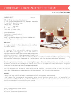
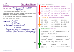


© Copyright 2026