
- PORTO - Publications Open Repository TOrino
Politecnico di Torino
Porto Institutional Repository
[Doctoral thesis] Development of refined models for multilayered composite
and sandwich structures: analytical formulation, FEM implementation and
experimental assessment
Original Citation:
L. Iurlaro (2015). Development of refined models for multilayered composite and sandwich
structures: analytical formulation, FEM implementation and experimental assessment. PhD thesis
Availability:
This version is available at : http://porto.polito.it/2606162/ since: May 2015
Published version:
DOI:10.6092/polito/porto/2606162
Terms of use:
This article is made available under terms and conditions applicable to Open Access Policy Article
("Creative Commons: Attribution-Noncommercial-No Derivative Works 3.0") , as described at http:
//porto.polito.it/terms_and_conditions.html
Porto, the institutional repository of the Politecnico di Torino, is provided by the University Library
and the IT-Services. The aim is to enable open access to all the world. Please share with us how
this access benefits you. Your story matters.
(Article begins on next page)
POLITECNICO DI TORINO
Doctoral Degree in Aerospace Engineering
Thesis
Development of refined models for multilayered
composite and sandwich structures
Analytical formulation, FEM implementation
and experimental assessment
Advisors
Prof. Marco DI SCIUVA
Prof. Marco GHERLONE
Author
Luigi IURLARO
XXVII Cycle, 2012-2014
“e volta nostra poppa nel mattino,
de' remi facemmo ali al folle volo”
(Dante Alighieri, Inferno, Canto XXVI)
Acknowledgements
First and foremost, I would like to express my sincere gratitude to Prof. Marco Di
Sciuva, my research advisor, that provided, during the years, insight, guidance and
motivation. All the time spent with him has been a precious occasion of cultural and
personal growth. It has been an honor and a pleasure to work with him. For his patient
guidance, suggestions and constant supports, I would like to thank Prof. Marco Gherlone,
my research co-advisor and friend. I am aware of all I owe to them.
I offer my sincere gratitude to Dr. Alexander Tessler, who provided fruitful suggestions
and interesting ideas, and to Dr. Massimiliano Mattone for his availability and excellent
solutions about experimental issues.
For the host period at the International Center for Numerical Methods in Engineering
(CIMNE), in Barcelona, I owe a special thanks, firstly, to Prof. Eugenio Oñate and to Prof.
Sergio Oller, and, secondly, to the CIMNE community made by extraordinary people.
Finally, the deepest gratitude is for my parents; without their unconditional love nothing
would have been possible. This work is dedicated to them.
Contents
1
Introduction
v
Preliminaries
ix
Theories for laminated plates
1
1.
Introduction . . . . . . . . . . . . . . . . . . . . . . . . . . . . . . . . . . . . . .
1
2.
Variational statement . . . . . . . . . . . . . . . . . . . . . . . . . . . . . . . . .
2
2.1
Virtual Displacement Principle . . . . . . . . . . . . . . . . . . . . . . . .
3
2.2
Reissner Mixed Variational Theorem . . . . . . . . . . . . . . . . . . . . .
4
Equivalent Single Layer Models . . . . . . . . . . . . . . . . . . . . . . . . . . .
5
3.1
Classical Laminated Plate Theory . . . . . . . . . . . . . . . . . . . . . . .
6
3.2
First-Order
. . . . . . . Shear
. . . .Deformation Theory . . . . . . . . . . . . . . . . . . . .
Higher-order
Theory . . . . . . . . . . . . . . . . . . .
. . . . . . . . Shear
. . . Deformation
. . .
6
Layer-wise
. . . Models
. . . . . . . . . . . . . . . . . . . . . . . . . . . . . . . . . . . . . . .
.Zigzag Models . . . . . . . . . . . . . . . . . . . . . . . . . . . . . . . . . . . . .
8
5.1
The choice of the zigzag function . . . . . . . . . . . . . . . . . . . . . . . .
10
Review
. . . . . . . . . . . . . . . . . . . . . . . . . . . . . .
. . . . .zigzag
. . . models
. .
Multiple
Method . . . . . . . . . . . . . . . . . . . . . . . . . . . . . . .
. . Models
. .
11
3.
3.3
4.
5.
5.2
6.
2
7
9
13
Refined Zigzag Theory
14
1.
Motivation . . . . . . . . . . . . . . . . . . . . . . . . . . . . . . . . . . . . . . .
14
2.
Refined Zigzag Theory for plates: displacements, strains and stresses . . . . . . . .
15
2.1
. . .
2.2
.Kinematic
. . . . . .assumptions
. . . . . . .. .. . . . .. .. .. . ... . . . . . . . . . . . . . . . . . . .
Refined
. . . . . zigzag function . . . . . . . . . . . . . . . . . . . . . . . . . . . . .
16
Non-linear
. . . . . strains and stresses . . . . . . . . . . . . . . . . . . . . . . . . .
Non-linear
. . . equations
. . . . . .of motion . . . . . . . . . . . . . . . . . . . . . . . . . . . .
20
3.1
25
2.3
3.
Linear bending . . . . . . . . . . . . . . . . . . . . . . . . . . . . . . . . .
i
17
21
4.
3.2
Free vibrations . . . . . . . . . . . . . . . . . . . . . . . . . . . . . . . . .
25
3.3
Linear buckling . . . . . . . . . . . . . . . . . . . . . . . . . . . . . . . . .
25
Extension of RZT to functionally graded structures. . . . . . . . . . . . . . . . . .
26
4.1
Refined zigzag function for functionally graded materials . . . . . . . . . . .
28
Governing
. . . . . . .equations
. . . . . . . . . . . . . . . . .. .. .. .. .. .. .. .. .. .. .. .. .. .. .. .. .. .. ..
First-order
. . . zigzag
. . . . models
. . . . .. .. .. .. . . . . . . . . . . . . . . . . . . . . . . . . . . .
5.1 Murakami’s zigzag function. . . . . . . . . . . . . . . . . . . . . . . . . . .
29
5.2
33
4.2
5.
3
Governing
. . . . . . .equations . . . . . . . . . . . . . . . . . . . . . . . . . . . . . .
34
1.
Introduction . . . . . . . . . . . . . . . . . . . . . . . . . . . . . . . . . . . . . .
34
2.
Reissner Mixed Variational Theorem . . . . . . . . . . . . . . . . . . . . . . . . .
37
(m)
RZT
kinematics and transverse shear stresses . . . . . . . . . . . . .
. . . . .plate
. . model:
. ..
3.1
. . . .Polynomial
. . . . . . assumption
. . . . . . .. .. .. .. .. .. . . . . . . . . . . . . . . . . . . . . . . .
3.2 Equilibrium-based assumption . . . . . . . . . . . . . . . . . . . . . . . . .
(m)
4.
RZT . governing
and constitutive relations . . . . . . . . . . . . . . . .
. . . . . . equations
. .
Appendix
. . . .1.. RZT
. . .integrated
. . . . . transverse
. . . . . shear stresses . . . . . . . . . . . . . . . . . . .
. . . . . . . . . . . . . . .
39
40
41
44
49
(3,2)-Mixed Refined Zigzag Theory
51
1.
Introduction . . . . . . . . . . . . . . . . . . . . . . . . . . . . . . . . . . . . . .
51
2.
Reissner Mixed Variational Theorem . . . . . . . . . . . . . . . . . . . . . . . . .
53
3.
Higher-order
. . . . . . . . . . . . . . . . . . . . . . . . . . . . . . . .
. . . . . . . .kinematics
..
3.1 Derivation of the zigzag function . . . . . . . . . . . . . . . . . . . . . . . .
54
Assumed
. . . . . . . . . . . . . . . . . . . . . . . . . . . . . .
. . transverse
. . . . . . stresses
. .
4.1
. . . .Transverse normal stress . . . . . . . . . . . . . . . . . . . . . . . . . . . .
57
4.2
59
5.
Transverse
shear stresses . . . . . . . . . . . . . . . . . . . . . . . . . . . .
. .
Governing
and constitutive relations . . . . . . . . . . . . . . . . . . . .
. . . equations
. . .
6.
Thermo-mechanical
. . . . . . . . . . . .beam
. . model . . . . . . . . . . . . . . . . . . . . . . . . . . .
67
4.
5
31
Mixed Refined Zigzag Theory
3.
4
30
. . . . . . .
56
57
64
Finite Elements Formulation
75
1.
Introduction . . . . . . . . . . . . . . . . . . . . . . . . . . . . . . . . . . . . . .
75
2.
Exact static stiffness RZT beam element . . . . . . . . . . . . . . . . . . . . . . .
76
2.1
. . . .Refined
. . . . Zigzag
. . . Theory for beams . . . . . . . . . . . . . . . . . . . . . . .
2.2 Consistent shape functions . . . . . . . . . . . . . . . . . . . . . . . . . . .
78
2.3
Mass
. . . .matrix,
. . . exact stiffness matrix and consistent load vector . . . . . . . .
(3,2)-Mixed Refined Zigzag Theory beam element . . . . . . . . . . . . . . . . .
82
3.1
Kinematic restatement . . . . . . . . . . . . . . . . . . . . . . . . . . . . .
84
3.2
Nine-nodes,
fifteen-dof’s anisoparametric element . . . . . . . . . . . . . .
. . . . .
Six-nodes, twelve-dof’s constrained anisoparametric element . . . . . . . . .
84
Temperature
. . . . . . . .field
. . representations
. . . . . . . . . . . . . . . . . . . . . . . . . . . . . . . .
stiffness matrix and consistent load vector . . . . . .
.Consistent
. . . . . mass
. . . matrix,
. .
87
3.
3.3
3.4
3.5
. . . . . . . . . . . . . . . . . . . . . . . . . . . .
ii
81
83
85
89
4.
(3,2)-Mixed Refined Zigzag Theory plate element . . . . . . . . . . . . . . . . . .
90
4.1
. . . .Kinematic
. . . . . .restatement
. . . . . . . . . . . . . . . . . . . . . . . . . . . . . . . . . . . 91
4.2 Eighteen-nodes,
thirty-six dof’s anisoparametric element . . . . . . . . . . . 92
. . . . .
4.3 Nine-nodes,
. . . . . . . twenty-seven
. . . . . . . dof’s
. . . constrained
. . . . . . anisoparametric element . . . . . 92
4.4
6
Consistent
. . . . . . mass
. . . matrix,
. . . . .stiffness
. . . . matrix
. . . . and
. . consistent
. . . . . load vector . . . . . .
Appendix 1. RZT-based beam finite element matrices . . . . . . . . . . . . . . . .
96
(m)
. . . . . . 2.. .RZT
. . (3,2)
. .-based
. . . .beam
. . finite element matrices . . . . . . . . . . . . . .
Appendix
103
(m)
Appendix 3. RZT(3,2)
-based plate finite element matrices . . . . . . . . . . . . . .
. . . . . . . . . . . . . . . . . . . .
104
Analytical results
106
1.
Introduction . . . . . . . . . . . . . . . . . . . . . . . . . . . . . . . . . . . . . .
106
2.
RZT assessment . . . . . . . . . . . . . . . . . . . . . . . . . . . . . . . . . . . .
107
2.1
Linear bending . . . . . . . . . . . . . . . . . . . . . . . . . . . . . . . . .
108
2.2
Free
vibrations . . . . . . . . . . . . . . . . . . . . . . . . . . . . . . . . .
.
.Linear buckling . . . . . . . . . . . . . . . . . . . . . . . . . . . . . . . . .
131
Mixed. Refined Zigzag Theory . . . . . . . . . . . . . . . . . . . . . . . . . . . .
3.1
bending . . . . . . . . . . . . . . . . . . . . . . . . . . . . . . . . .
. . . .Linear
.
143
3.2
Free
vibrations . . . . . . . . . . . . . . . . . . . . . . . . . . . . . . . . .
.
(3,2)-Mixed
Refined Zigzag Theory . . . . . . . . . . . . . . . . . . . . . . . . .
.
147
4.1
. . . .Linear
. . . .bending . . . . . . . . . . . . . . . . . . . . . . . . . . . . . . . . .
Appendix
. 1. Mechanical properties of materials and stacking sequences . . . . . .
150
2.3
3.
4.
Appendix 2. Functionally graded sandwich plates: mechanical properties and
stacking sequences . . . . . . . . . . . . . . . . . . . . . . . . . . . . . . . . . . .
7
138
143
150
157
159
Finite Element results
162
1.
Introduction . . . . . . . . . . . . . . . . . . . . . . . . . . . . . . . . . . . . . .
162
2.
Exact static stiffness RZT beam element . . . . . . . . . . . . . . . . . . . . . . .
163
2.1
. . . .Static
. . . analysis
. . . . . . . . . . . . . . . . . . . . . . . . . . . . . . . . . . . . .
2.2 Free vibrations analysis . . . . . . . . . . . . . . . . . . . . . . . . . . . .
163
(3,2)-Mixed
Zigzag Theory-based beam element . . . . . . . . . . . . .
. . . . Refined
.
3.1 Convergence . . . . . . . . . . . . . . . . . . . . . . . . . . . . . . . . .
167
3.2
Static analysis . . . . . . . . . . . . . . . . . . . . . . . . . . . . . . . . .
172
3.3
Dynamic response . . . . . . . . . . . . . . . . . . . . . . . . . . . . . . .
178
(3,2)-Mixed
Refined Zigzag Theory-based plate element . . . . . . . . . . . . .
. .
4.1 Convergence . . . . . . . . . . . . . . . . . . . . . . . . . . . . . . . . . .
180
4.2
Static analysis . . . . . . . . . . . . . . . . . . . . . . . . . . . . . . . . .
183
4.3
Free vibrations analysis . . . . . . . . . . . . . . . . . . . . . . . . . . . .
187
3.
4.
8
98
.. . . . . .
166
167
180
Experimental assessment
189
1.
Introduction . . . . . . . . . . . . . . . . . . . . . . . . . . . . . . . . . . . . .
189
2.
Specimens . . . . . . . . . . . . . . . . . . . . . . . . . . . . . . . . . . . . .
190
iii
3.
4.
5.
Materials characterization . . . . . . . . . . . . . . . . . . . . . . . . . . . . . .
190
3.1
Mass density . . . . . . . . . . . . . . . . . . . . . . . . . . . . . . . . .
192
3.2
Young’s modulus and Poisson’s ratio . . . . . . . . . . . . . . . . . . . . .
192
Four-points bending test . . . . . . . . . . . . . . . . . . . . . . . . . . . . . . .
198
4.1
Experimental set-up . . . . . . . . . . . . . . . . . . . . . . . . . . . . . .
198
4.2
Results . . . . . . . . . . . . . . . . . . . . . . . . . . . . . . . . . . . . .
200
Hammer test . . . . . . . . . . . . . . . . . . . . . . . . . . . . . . . . . . . . .
203
5.1
Experimental set-up . . . . . . . . . . . . . . . . . . . . . . . . . . . . . .
203
5.2
Results . . . . . . . . . . . . . . . . . . . . . . . . . . . . . . . . . . . . .
204
Summary and conclusions
209
References
213
iv
Introduction
Over the last three decades, composite materials have been increasingly used in
different engineering field (military and civilian aircraft, aerospace vehicles, naval and
civil structures) due to their high stiffness-to-weight and strength-to-weight ratios.
Nowadays, relatively thick laminated composite and sandwich materials with one hundred
or more layers find their applications in primary load-bearing structural components of the
modern aircraft. To ensure a reliable design and failure prediction, accurate evaluation of
the strain/stress state is mandatory.
A high-fidelity analysis of multilayered composite and sandwich structures can be
achieved by adopting detailed 3D finite element models that turn into a cumbersome
modeling at high computational cost. Thus, most of the researchers efforts are devoted to
the development of approximated models wherein assumptions on the distribution of
displacements and/or stresses are made, thus reducing the 3-dimensional analysis to a 2dimensional problem. Generally speaking, three kinds of 2D approximated models are
available: Equivalent Single Layer models, Layer-wise theories and the Zigzag models.
Even if computationally efficient, the Equivalent Single Layer models are not accurate in
terms of local response prediction; the Layer-wise theories, that on the contrary ensure
great accuracy, are computationally very expensive. In the ‘80s, thanks to the original
works by Prof. Di Sciuva, a new modeling strategy of multilayered composite and
sandwich structures arose: the so-called Zigzag theories, wherein accuracy comparable
with that proper of the Layer-wise models is achieved but saving the computational cost.
Inspired by early Prof. Di Sciuva’s works, many researchers developed Zigzag models in
v
the course of these thirty years, contributing to progress in the multilayered composite and
sandwich structures modeling field.
For accuracy, computational cost and efficient finite element implementation, the most
remarkable Zigzag model, inspired by the Prof. Di Sciuva’s work, is the Refined Zigzag
Theory, recently developed by Dr. Tessler, Prof. Di Sciuva and Prof. Gherlone. From its
first appearance, the Refined Zigzag Theory has experienced several developments in
terms of beam and plate finite element implementations and has been extensively assessed
on static problems. Other researchers, by using the Refined Zigzag Theory as basis,
developed models with higher-order kinematics and including secondary effects as the
normal deformability one, obtaining fair results.
In this context, the present research work is motivated, first of all, by the necessity to go
further into the investigation about the Refined Zigzag Theory prediction capabilities, to
highlight and solve possible flaws and to develop an original higher-order zigzag model
able to produce accurate results in those situations wherein the Refined Zigzag Theory is
not adequate. Taking in mind the motivation of the present research work, the Thesis is
organized following a logical (and chronological) order.
Chapter 1 is devoted to a detailed discussion and review of models for the analysis of
multilayered composite and sandwich structures, highlighting merits and deficiencies.
In Chapter 2, the Refined Zigzag Theory for plates is briefly recalled. For the first time,
the non-linear governing equations are obtained and specialized to the linear bending,
undamped free vibrations and linear buckling problems. Moreover, due to the growing
interest towards the advanced functionally graded materials, the Refined Zigzag Theory is
extended to the analysis of multilayered plates embedding functionally graded layers.
Finally, a comparison of the Refined Zigzag function with the Murakami’s one is set.
In Chapter 3, the first substantial attempt to enhance the Refined Zigzag Theory is
made. Based on the Reissner Mixed Variational Theorem, the Mixed Refined Zigzag
Theory is developed in order to improve the constitutive transverse shear stresses
prediction and, as consequence, the transverse shear stiffness estimation.
The formulation of a novel higher-order zigzag model (called (3,2)-Mixed Refined
Zigzag Theory), originated by the Refined Zigzag Theory, is introduced in Chapter 4,
wherein the discussion is focused on plate problems. Moreover, an extension to the
thermo-mechanical analysis, but limited to the beam problems for sake of conciseness, is
presented. Based on the Reissner Mixed Variational Theorem, the novel higher-order
zigzag model includes the transverse normal deformability effect, by extending the
vi
transverse displacement approximation with respect to the Refined Zigzag Theory, and the
transverse normal stress, neglected in the Refined Zigzag Theory. The kinematics, in terms
of in-plane displacements assumption, is also enriched with respect to the Refined Zigzag
Theory. The formulation of the novel higher-order zigzag model is motivated by the need
of a computational model able to accurately analyze the response of thick multilayer
composite beams/plates wherein secondary effects (the higher-order displacements patterns
along the thickness, the transverse normal deformability and the transverse normal stress),
neglected by the Refined Zigzag Theory, become significant.
Finite elements implementations are the subject of Chapter 5. Firstly, a novel Refined
Zigzag Theory-based beam element, employing exact static shape functions, is presented.
Secondly, a (3,2)-Mixed Refined Zigzag Theory-based beam element suitable for a
thermo-mechanical analysis of thick multilayered composite and sandwich beams is
formulated. Later, a (3,2)-Mixed Refined Zigzag Theory-based plate element is introduced.
Chapters 6 and 7 are devoted to the numerical results. In Chapter 6, only analytical
solutions, that is exact or approximated ones by using the Rayleigh-Ritz’s method, are
presented. A in-deep investigation of the Refined Zigzag Theory prediction capabilities in
problems concerning the linear bending, free vibrations and buckling problems of
multilayered composite and sandwich plates, also including functionally graded layers, is
carried out. To assess the improvements of the Mixed Refined Zigzag Theory with respect
to the original displacement-based model formulation, the linear bending and free
vibrations problems of laminated composite and sandwich plates are taken into
consideration. Finally, the (3,2)-Mixed Refined Zigzag Theory performances are tested on
the bending problem of a thick laminated composite plate. The finite element results,
collected in Chapter 7, are devoted to the assessment of the RZT-based beam element
employing exact static shape functions, both on static and free vibrations problems, and
comparing the results with those obtained by means an already developed beam element
based on the same underlying theory. The (3,2)-Mixed Refined Zigzag-based beam and
plate elements, once their convergence is proved, are used to solve static and dynamic
problems.
Finally, in Chapter 8, the results of an experimental campaign acted out are presented
along with the experimental set-up used. The tests concern the four-point bending test of
sandwich beams, for the static analysis, and hammer test on cantilever sandwich beams, for
the free vibrations problems. The experimental results are compared with those obtained
by using the Refined Zigzag Theory-based beam element as further theory assessment.
vii
The present research activity supports the great accuracy of the Refined Zigzag Theory
and for this reason deals with some overlooked aspects, as the application to the
functionally graded materials (Chapter 2), the mixed formulation (Chapter 3), the
implementation of a beam finite element employing exact static shape functions (Chapter
5) and the correlation with experimental results (Chapter 8). By enriching the Refined
Zigzag Theory and using the Reissner Mixed Variational Theorem, a novel higher-order
mixed zigzag model, called (3,2)-Mixed Refined Zigzag Theory is developed (Chapter 4).
The higher-order zigzag model constitutes the underlying theory for a beam finite element,
suitable for a thermo-mechanical analysis, and a plate element, formulated taking into
account only mechanical loads. The results presented (Chapters 6-8), along with those
already published in the open literature by other authors, still encourage the use of the
Refined Zigzag Theory in the analysis of relatively thick multilayered composite and
sandwich structures. Moreover, when the transverse normal stress and the transverse
normal deformability effects are not negligible, the (3,2)-Mixed Refined Zigzag Theory
appears proficient to solve these cases in virtue also of its efficient finite element
implementations.
The author’s auspice is that the models belonging to the Refined Zigzag Theory class
becomes to attract attention of the companies involved in the design and analysis of
multilayered composite and sandwich structures and of the finite element commercial
codes that still implemented models not suitable for the analysis of composite and
sandwich structures, as extensively demonstrated.
viii
Preliminaries
The objective of this section is to briefly review some basic equations, concerning the
mechanics of orthotropic materials, that are abundantly used in the theoretical
developments. Many details, above all about the mathematics, are omitted and the
interested reader can refer to [Reddy, 2004] for a complete discussion.
Strain-displacement relations
Consider a deformable body of known geometry, constitution, load and boundary
conditions. Each material points of the body is referred to a Cartesian coordinate system
(x1,x2,x3) and the Cartesian components of the displacement vector u are U i where the
Latin index takes values 1, 2 and 3.
According to the standard solid mechanics [Reddy, 2004], the strain is measured by
using the Green-Lagrange strain tensor E, that is defined in terms of displacement
gradients as [Reddy, 2004]
1
T
T
E u u u u
2
(P.1)
Performing the dot product, the orthogonal components of the Green-Lagrange tensor
are given by
E jk
1
kU j jU k jUi kUi
2
ix
(P.2)
where the notation i is used to denote the derivative with respect to the coordinate xi. If
the displacement gradient is small, that is u 1 , the E tensor reduces to the
infinitesimal strain tensor, , which components read as
ij
1
iU j jUi
2
(P.3)
Constitutive material law
Herein, the constitutive equation of linear elasticity for the case of infinitesimal
deformation of an orthotropic material, referred to as the Hooke’s law, is discussed.
Denoted with σ the stress tensor, the material constitutive law reads as [Reddy, 2004]
ij Cijkl kl
(P.4)
where Cijkl is the fourth-order tensor of material parameters, called stiffness tensor, and for
an orthotropic material it depends on nine independent coefficients.
With reference to Eq. (P.4), a plane stress state with respect to the x1-x2 plane is
characterized by the following condition
33 0
(P.5)
The constitutive material law, according to the plane stress state, reads as
C
3 C 3 3 3
(P.6)
where the Greek index takes values 1 and 2 and 3 is the engineering transverse shear
strain, defined as 3 2 3 . In Eq. (0.6), the reduced stiffness coefficients, C , appear
and read as
C C
C 33C 33
C3333
(P.7)
whereas the stiffness coefficients related with the transverse shear stresses are not affected
by the plane-stress assumptions. For these stiffness coefficients, since the subscript
depends only on two indices, a different notation is adopted: Q C 3 3 .
x
It is worth to note that, by making use of Eq. (P.6), it is possible to state in an equivalent
way, called mixed form, the constitutive law, Eq. (P.4). By introducing the compliant
1
coefficient, S33 C3333
, the constitutive material law in mixed form reads as
C S33 R 33
3 Q 3
(P.8)
33 S33 33 S33 R
wherein R C 33 .
When the thermal effect due to a temperature variation, T T0 , with respect to a
reference one, T0 , has to be taken into consideration, the constitutive law is enriched by the
thermal contribution and the mixed form of the constitutive law, Eq. (P.8), becomes
[Gherlone et al., 2007]
C S33 R 33
3 Q 3
(P.9)
33 S33 33 S33 R S3333
where S3333 R and ij Cijkl kl with kl denoting the thermal expansion
coefficients in the geometric axes.
xi
Chapter 1
Theories for laminated plates
1. Introduction
In the last thirty years, composite materials have been increasingly used in many
industrial applications due to their high specific mechanical properties, reduced weight,
high corrosion and fatigue resistance. Along with these positive aspects, multilayered
composite structures offer the possibility to tailor the mechanical properties according to
the specific application by choosing carefully the fiber orientation and the stacking
sequence. In aerospace field, the increasing use of composite and sandwich materials for
primary load bearing structural components requires computational tools able to accurately
predict the stress field in order to achieve reliable design and failure analysis. In particular
near the geometric singularities, like as holes or free edges, where the stress field becomes
three-dimensional and stress intensity factors arise, the computational model has to be very
accurate, above all on the prediction of the transverse stresses, due to the key role played
by them in damage mechanisms like as debonding and delamination.
It is trivial to note that the actual stress field in multilayered composite structures can be
computed by exact Elasticity-based solutions. In the open literature, several exact solutions
are available: Pagano [Pagano, 1969; Pagano, 1970] developed exact solutions for crossply and sandwich plates in the framework of linear Elasticity; Srinivas and Rao [Srinivas et
Chapter 1 – Theories for laminated plates
al., 1970; Srinivas et al., 1971] obtained exact solution for the static and dynamic analysis
of thick laminates; Noor and Burton [Noor et al., 1990], Savoia and Reddy [Savoia et al.,
1992] published solutions for cross-ply and antisymmetric angle-ply rectangular plates. It
is easy to note that exact Elasticity solutions are available only for a limited set of
geometries, loads and boundary conditions (in the case of plates, mainly bi-sinusoidal
transverse pressure and simply support boundary condition). By using the Fourier series,
the exact Elasticity solution can be easily extended to case of a plate with a general load.
When an exact solution is not available, stress analysis can be performed by high-fidelity
3D finite elements models that turns out to be accurate but computationally expensive.
From this point of view, an interesting solution is to develop approximate 2D models: in
these models, the distribution along one of the coordinate axes of the reference frame is
assumed for the primary variables, thus reducing a 3D problem to a 2D one. In the
framework of the displacement-based plate/shell models, the through-the-thickness
distribution of displacement components is assumed whereas the behavior of the elastic
body in the plane generated by the remaining two coordinate axes is recovered by solving
the governing equilibrium equations along with the variationally consistent boundary
conditions.
In this chapter, the models formulated for the analysis of multilayered composite and
sandwich plate/shell structures are examined following a common accepted classification
[Reddy, 2004]. The models can be divided into (i) displacement-based models, wherein the
primary variables are only the displacement components on which the assumptions are
made; and (ii) mixed models, wherein displacements and stresses are assumed
independently. Along with this classification, the plate/shell models can be divided into (a)
Equivalent Single Layer (ESL) models and (b) Layer-wise (LW) ones, according to the
type of kinematics assumed. In the former class of structural theories, the kinematics
assumed is C1-continuous, that is the displacement components and their derivatives are
assumed to vary continuously along the plate/shell thickness. This means that the
multilayer structure is substituted with a plate/shell made by an equivalent single layer. On
the contrary, LW models postulates a C0-continuous kinematics, that is a distribution of
displacements (first of all, in-plane displacements) continuous along the thickness with
first order derivatives showing a jump at layer interfaces (the reason of this discontinuity
will be explained hereinafter). Moreover, according to [Ghugal et al., 2002] the LW
models are further divided into (a) layer dependent, wherein the number of kinematic
variables increases with the number of layers; and (b) layer independent, wherein the
2
Chapter 1 – Theories for laminated plates
number of variables remains constant and independent on the number of layers. A
particular class of LW layer independent models are the so-called Zigzag (ZZ) models. In
this context, the terminology “layer-wise models” is used to indicate only the layer
dependent LW theories, whereas the ZZ models are treated separately.
2. Variational statement
According to the classification before mentioned, the plate/shell models can be divided
into displacement-based and mixed models, depending on the type of primary variables.
This difference reflects also the variational principle on which the model is formulated. In
fact, displacement-based models are formulated via the Virtual Displacements Principle
[Reddy, 2004] whereas mixed models are developed using the Reissner Mixed Variational
Theorem [Reissner, 1950]. In this paragraph, the two variational statement are briefly
recalled.
2.1. Virtual Displacements Principle
All the displacement-based models are formulated via the Virtual Displacement
Principle. Omitting many details that the reader can find in [Reddy, 2004], it is important to
remark that the Virtual Displacements Principle is the weak form of the 3D Elasticity
equations that are solved by assuming as arbitrary test functions the virtual displacements
[Zienkiewicz et al., 2000]. In formula, the principle reads as
ε σd u bd u td 0
T
T
T
(1.1)
where , are the body volume and the external surface, respectively; ε, σ are the strain
and stress vectors and u contains the displacement components. The body forces and the
external surface applied loads are quoted as b, t , respectively. Recognizing the virtual
variation of the strain energy, U , the virtual variation of the work done by inertial forces,
Wi , and that done by external applied loads, W , the Virtual Displacement Principle
appears also as
U Wi W 0
(1.2)
that represents the common way to present the Principle of Virtual Work (D’Alembert’s
Principle).
3
Chapter 1 – Theories for laminated plates
When a displacement-based model is developed, the only primary variables are the
displacements thus the strain field and the stress one come from the strain-displacement
relations and the constitutive material law, respectively.
2.2. Reissner Mixed Variational Theorem
In the framework of multilayered composite structures modeling, an important role is
played by the Reissner Mixed Variational Theorem [Reissner, 1950], since it allows for an
independent assumption on displacements and transverse shear and normal stresses. It is
interesting to note that the Reissner Mixed Variational Theorem is a particular case of a
more general two-field variational principle, the Hellinger-Reissner one [Hellinger, 1914]
that allows independent assumption on displacements and all the six stress tensor
components. Details about the two principles can be found in [Zienkiewicz et al., 2000]; in
this context the Reissner Mixed Variational Theorem is stated and the quantities involved
explained. The above cited theorem reads as
ε σd τ γ γ d
T
aT
a
a
33
33a d
(1.3)
u bd u td 0
T
33
T
a
where τ a , 33
denote the assumed transverse shear and normal stresses, respectively, while
γ a , 33a denote the transverse shear and normal strains coming from the constitutive
a
relations, using τ a , 33
. The counterpart, that is the strain coming from the strain-
displacement relations, are denoted as γ, 33 . It is important to remark that, in this case, the
stress vector σ contains, for the transverse shear and normal stress part, the assumed
stresses.
Due to the arbitrary virtual variation of the stress variables, the solution procedure of the
Reissner Mixed Variational Theorem leads the compatibility terms between the strains
coming from the assumed displacements and those coming from the constitutive equations
to be solved in a form wherein the integration is limited to the plate thickness,
henceforward called weak form, that is
τ aT γ γ a 0
33a 33 33a 0
4
(1.4)
Chapter 1 – Theories for laminated plates
wherein the ... notation stands for the integration over the entire thickness.
By solving the compatibilities, Eq. (1.4), the assumed stresses are expressed in terms of
the kinematic variables, thus reducing the complexity of the model.
3. Equivalent Single Layer Models
The Equivalent Single Layer models, called also Smeared models, assume a C1continuous distribution along the thickness of displacements. In this way, the ESL models
substitute the multilayered plate/shell with an equivalent single layer plate/shell. Due to
this feature, the ESL models are generally an extension to multilayered structures of the
models developed for homogeneous isotropic plates/shells.
The typical assumption of an ESL model for a generic displacement component,
ui (x, z, t ) , reads as
N
ui (x, z, t ) f j ( z )ui( j ) (x, t )
(1.5)
j 0
where f j ( z ) represents the base functions of the through-the-thickness assumption of the
displacement component ui (x, z, t ) and ui( j ) (x, t ) are the model kinematic variables that are
determined by solving the governing equations and the variationally consistent boundary
conditions.
Generally speaking, as base functions, powers of the thickness coordinate, that is
f j ( z ) z j , are chosen and depending on the maximum order in the polynomial expansion,
it is possible to distinguish between first-order ELS models and higher-order ESL ones. In
the open literature are also available ESL models adopting the trigonometric functions as
base for the through-the-thickness distribution of displacements. In the framework of the
trigonometric ESL models, are noticeable the works done by Touratier [Touratier, 1991]
that, to the best author knowledge, was the first to adopt trigonometric functions in
smeared models.
It is not intent of this paragraph to carry out a detailed review of ESL models, thus the
author addresses the interested reader to review works [Ghugal et al., 2002; Wanji et al.,
2008; Khandan et al., 2012].
5
Chapter 1 – Theories for laminated plates
3.1. Classical Laminated Plate Theory
The Classical Laminated Plate Theory (CLPT) represents the extension to multilayered
plates of the Classical Plate Theory (CLT) developed by Kirchhoff for isotropic plates. It is
the simplest ESL model and the assumed kinematics reads as
U (x, z, t ) u (x, t ) z w(x, t )
U z (x, z, t ) w(x, t )
(1.6)
where the subscript 1, 2 . Consistent with the kinematic assumptions of the CLPT,
u , w represent the in-plane and transverse displacements of a point located on the
reference plane (i.e., z 0 ) of the plate. The kinematics in Eq.(1.6) implies that the crosssection remains plane after deformation and transverse shear and normal deformations are
neglected, thus accounting only for bending and in-plane stretching.
It is well-known the role played by the transverse shear stresses on the plate/shell
structural response. Neglecting the transverse shear effect leads to relevant errors: for the
isotropic plate, the CLPT can be applied when the span-to-thickness ratio of the plate is
a/2h > 30 (that is, for thin plate); for a multilayered laminate, the minimum value of the
span-to-thickness ratio that justifies the application of the CLPT increases up to 50. Along
with the span-to-thickness ratio, the application of the CLPT depends also on the stiffness
ratio between the adjacent layers: the use of the CLPT for highly heterogeneous stacking
sequences leads to relevant errors, even if the span-to-thickness ratio is greater that 50.
3.2. First-Order Shear Deformation Theory
The First-Order Shear Deformation Theory (FSDT) [Whitney et al., 1970] represents the
extension to the multilayered laminate of the Reissner-Mindlin plate theory [Mindlin,
1951; Reissner, 1945]. With respect to the CLPT, the FSDT relaxes the hypothesis
suggested by Kirchhoff allowing a transverse shear deformation of the plate. The
kinematics of the FSDT reads as
U (x, z, t ) u (x, t ) z (x, t )
U z (x, z, t ) w(x, t )
(1.7)
where represents the rotation around the x coordinate axis.
Consistent with the displacement field in Eq. (1.7), the transverse shear strain is
assumed constant along the plate thickness, thus yielding to a piece-wise constant
6
Chapter 1 – Theories for laminated plates
distribution of transverse shear stress that violates the Elasticity conditions at layer
interfaces. Moreover, since the distribution is constant along the thickness, the zerotransverse shear stresses condition at the top and bottom plate surface is not satisfied. The
gap between the transverse shear stresses distribution provided by the FSDT and that
obtained by the Elasticity requires the use of a shear correction factor [Whitney, 1973;
Vlachoutsis, 1992; Hutchinson, 2001] in the FSDT that acts reducing the shear stiffness of
the plate. The shear correction factor estimation is not easy since it depends on the stacking
sequence, the geometry and the boundary and loading conditions.
By the inclusion of the transverse shear effect, the FSDT could be able to provide
moderately accurate global responses (maximum deflection, first natural frequency and
buckling load) if an adequate shear correction factor is adopted and the plate features a
span-to-thickness ratio a/2h > 20. Although the global responses are moderately accurate,
the through-the-thickness distribution of displacements and stresses for a multilayered
plate deviates from that provided by the exact solution due to the FSDT through-thethickness C1-continuity kinematic assumptions.
3.3. High-Order Shear Deformation Theory
As remarked before, the inclusion of the transverse shear effect in the FSDT guarantees
an increase in accuracy, on condition that the plate remains thin. By increasing the plate
thickness, the through-the-thickness linear distribution of the displacements provided by
the FSDT is no more correct as suggested by the Pagano exact Elasticity solution [Pagano,
1969; Pagano, 1970]. In fact, the thickness effect acts making the displacements
distribution non-linear along the thickness and requires a description with a higher-order
polynomial.
The term High-Order Shear Deformation Theory (HSDT) refers to a set of ESL models
adopting a polynomial assumption for the displacements with a order greater than one. The
reader can refer to [Ghugal et al., 2002; Wanji et al., 2008; Khandan et al., 2012] for a
detailed review of the HSDTs.
A fundamental contribution in the framework of HSDTs was given by the third-order
shear deformation theory developed by Reddy [Reddy, 1984; Reddy, 1990] and assuming
the following kinematics
7
Chapter 1 – Theories for laminated plates
4
U (x, z, t ) u (x, t ) z (x, t ) z 3 2 w
3h
U z (x, z, t ) w(x, t )
(1.8)
The transverse shear stresses distribution provided by this model is parabolic along the
thickness direction and able to satisfy the zero-transverse shear stresses condition on the
top and bottom plate surface. For this reason, the model does not require any shear
correction factors. It is worth to note that, due to smeared-type approximation of
displacements, the transverse shear stresses are discontinuous at the interface between two
layers with different mechanical properties.
4. Layer-wise Models
The multilayered composite structures are characterized by a severe transverse
anisotropy since they are made by the superposition of considerably different layers. The
transverse anisotropy is responsible for the zigzag effect, that is, the distribution along the
thickness of in-plane displacements is not C1-continuous but C0-continuous, showing a
change in the slope at layer interfaces. The jump of the first-order derivative with respect
to the thickness coordinate of the in-plane displacement at layer interface derives from
equilibrium consideration: according to the Cauchy’s theorem, the transverse shear stresses
have to be equal at layer interfaces. The unique way to ensure a continuity condition on
these stresses having layers with different mechanical properties is to ensure a jump in the
transverse shear strains, obtainable with a discontinuous first-order derivative of in-plane
displacements with respect to the thickness coordinate at layer interfaces. It is easy to
understand that the zigzag effect is the main responsible for the inaccuracy of the ESL
models in predicting the local (through-the-thickness distribution of displacements and
stresses) and global (maximum deflection, natural frequencies and buckling load) response
of multilayered structures.
The problem of reproducing a C0-continuous displacement field along the thickness can
be addressed by adopting LW models, wherein an ESL-like assumption is made for every
single layer. According to Reddy [Reddy, 2004], the LW models are divided into partial
theories and full theories: the former assume a C0-continuous distribution only for the inplane displacements; on the contrary, the latter ones include the zigzag effect also in the
transverse displacement assumption. The purpose of this paragraph is only to explain the
8
Chapter 1 – Theories for laminated plates
basic idea of the LW theories, without giving a detailed review. Readers interested may
refer to [Ghugal et al., 2002; Wanji et al., 2008; Khandan et al., 2012].
For the sake of simplicity, partial LW models are taken into consideration. A typical
displacements assumption of a partial LW model reads as
U( k ) (x, z, t ) u( k ) (x, t ) z( k ) (x, t ) .... z n( k ) ( x, t )
U z( k ) (x, z, t ) w(x, t )
(1.9)
where the superscript (k) means that the quantities are referred to the kth layer. As Eq. (1.9)
shows, the LW models adopt for each layers an ESL-like assumption with a polynomial
degree up to n. Along with the assumption of Eq. (1.9), the continuity conditions on
displacements and transverse stresses have to be satisfied at layer interfaces. These contact
conditions only reduce the total number of kinematic variables that still remains dependent
on the number of layers.
With LW models, high accuracy is obtained at the expense of a substantial
computational cost that increases with the number of layers. This makes the LW models
inadequate for the analysis of multilayered structures made by one hundred or more layers,
as the structures for real applications are.
5. Zigzag Models
The basic idea of the Zigzag models, pioneered by Di Sciuva [Di Sciuva, 1983; Di
Sciuva, 1984a,b; Di Sciuva, 1986] is to model the actual cross-section distortion typical of
multilayered structures by using a limited and fixed number of kinematic variables, in
order to preserve the computational cost. The kinematics of a Zigzag model can be
presented in a multi-scale view: the assumed displacement field is given by the
superposition of a coarse kinematics and a fine one. The former represents the behavior on
the total laminate thickness scale whereas the fine kinematics describes the behavior on the
layer thickness scale. An ESL model is adequate to constitute the coarse kinematics due to
the C1-continuous assumption. The layer refinement, that is the fine kinematics, is given by
the product of a priori known piecewise continuous function of the thickness coordinate,
called zigzag function, and a kinematic variable function of the in-plane coordinate axes,
called zigzag amplitude, that rules the magnitude of the zigzag effect. In this way, a Zigzag
model retains the same kinematic variables of the ESL model adopted for the coarse
kinematics in addition to the zigzag amplitudes, one in each directions, thus resulting in a
constant number of the kinematic-variables model.
9
Chapter 1 – Theories for laminated plates
The typical Zigzag kinematics (for the sake of simplicity, constant transverse
displacement distribution and ESL coarse kinematics with polynomial basis functions are
considered) reads as
U( k ) (x, z, t ) u (x, t ) z (x, t ) .... z n (x, t ) ( k ) ( z ) ( x, t )
U z( k ) (x, z, t ) w(x, t )
(1.10)
where the Greek subscript takes values 1, 2 and u (x, t ), (x, t ),...., (x, t ) represent
the kinematic variables of the coarse kinematics, ( k ) ( z ) the zigzag function and (x, t )
the zigzag amplitude. On the whole, the Zigzag model in Eq. (1.10) has 2(n+1)+1
kinematic variables coming from the coarse kinematics plus two zigzag amplitudes, giving
a constant 2(n+1)+3 number of variables irrespective of the number of layers.
5.1. The choice of the zigzag function
Once the ESL model describing the coarse kinematics has been chosen, the fundamental
step in the development of a Zigzag model is the choice of the zigzag function: the
predictive capabilities of models assuming the same ESL coarse kinematics depend on the
zigzag function. In the open literature, two kind of zigzag functions are available: the
former is the Di Sciuva’s zigzag function [Di Sciuva, 1983; Di Sciuva, 1984a,b; Di Sciuva,
1986] originally developed in the framework of a displacement-based zigzag model; the
second one, attributed to Murakami [Murakami, 1986], was introduced, for the first time,
in the framework of a Reissner Mixed Variational Theorem-based zigzag model.
The Di Sciuva’s zigzag function is physically-based since it is formulated in order to
satisfy, a priori, the continuity conditions of transverse shear stresses at layer interfaces.
The fulfillment of continuity of transverse shear stresses leads the zigzag function to be
defined on the basis of the mechanical proprieties of the layers and changes accordingly
the stacking sequence.
On the contrary, Murakami derived his zigzag function examining the distribution along
the thickness of the in-plane displacements of a periodic laminate, that is a laminate
featuring a stacking sequence made by the succession of the same two materials. As the
exact Elasticity solution suggests, in this case the through-the-thickness distribution of inplane displacements shows a periodicity also in the slope change, that is the same in
magnitude but opposite in sign from an interface to the subsequent one. The Murakami’s
10
Chapter 1 – Theories for laminated plates
zigzag function is defined in order to reproduce this periodic behavior and for this reason is
no mechanical properties-dependent.
For a long time, the Di Sciuva and Murakami zigzag functions have been involved in
the development of zigzag models, both displacement-based and mixed ones, without an
in-deep investigation and comparison of the predictive capabilities of the zigzag functions
being performed. Recently, Gherlone [Gherlone, 2013] has covered this lack in the open
literature, carried out a comparison of the two zigzag functions in the framework of a firstorder zigzag model, that is a model assuming the FSDT as coarse kinematics, both
displacement-based and mixed one, focusing on the elasto-static response of multilayered
composite and sandwich beams. The conclusion of the investigation performed by
Gherlone states the superior predictive capabilities of the Di Sciuva’s zigzag function over
the Murakami’s one. The same conclusions made by Gherlone [Gherlone, 2013] have been
lately confirmed by Iurlaro et al. [Iurlaro et al.,2014a] also for the static, free vibrations
and buckling load problems of sandwich plates.
For a detailed description of the zigzag functions and their use in the development of a
First-Order Zigzag model, see Chapter 2.
5.2. Review zigzag models
The research activity of this Thesis focuses on Zigzag models and for this reason the
author considers worthwhile a review of the main works done in the last thirty years,
distinguishing the Zigzag models on the basis of the zigzag function employed.
As pioneer of Zigzag theories, of remarkable importance are the works done by Di
Sciuva. In addition to the already cited early work [Di Sciuva, 1983; Di Sciuva, 1984a,b],
it is important to mention the paper published in the framework of a linear zigzag model
[Di Sciuva, 1984a,b; Di Sciuva, 1986; Di Sciuva, 1987] and in the framework of the cubic
zigzag model [Di Sciuva, 1990; Di Sciuva, 1992; Di Sciuva, 1994; Di Sciuva, 1997] by the
same author. While the Di Sciuva’s linear zigzag model is obtained as refinement of the
FSDT, the cubic one is formulated starting from the Reddy’s third-order shear deformation
theory and is able to satisfy a priori the continuity of transverse shear stresses at layer
interfaces and the zero-conditions at the top and bottom plate surfaces. The Di Sciuva’s
cubic zigzag model is further developed in order to represent the interlaminar slip that
occurs at damage interface [Di Sciuva, 1997]. Inspired by the Di Sciuva’s works, many
zigzag model arose. In the framework of cubic models, a contribution was given by Cho
and Parmenter [Cho et al., 1993] and recently by Nemeth [Nemeth, 2012]. By using the
11
Chapter 1 – Theories for laminated plates
sublaminates approach, a 3D finite element based on a linear zigzag model accounting for
a linear distribution across the sublaminate thickness of a transverse displacement was
formulated by Cho [Cho et al., 2000]. An important contribution in the development of
zigzag models was given by Icardi: in [Icardi, 2001a,b; Icardi, 2005] a higher-order zigzag
model accounting for a piece-wise cubic distribution of in-plane displacements and
piecewise four-order distribution of transverse displacement is developed. The transverse
shear and normal stresses continuity conditions are not sufficient and the continuity
condition on the gradient of transverse normal stress is enforced at layer interfaces. In
[Icardi, 2011] an adaptive approach is proposed: the assumed kinematics can be refined
with higher-order terms in order to improve locally the solution, where necessary. The
coupled thermo-electro-mechanical analysis by using Zigzag models are performed in
[Kapuria et al., 2003; Topdar et al., 2004; Kapuria et al., 2004]. In [Oh et al., 2005] a
cubic zigzag model able to solve the elasto-dynamic equations of multilayered composite
plates with multiple delaminations is presented. Examples of trigonometric ESL model in
conjunction with Di Sciuva’s zigzag function can be found in [Vidal et al., 2006; Arya et
al., 2002]. A cubic zigzag model, very similar to the Di Sciuva’s one, is developed in
[Xiaohui et al., 2011; Xiaohui et al., 2012] and a finite element not requiring the continuity
of the first order derivative of the transverse displacement is formulated. Interesting is the
predictor-corrector approach introduced in [Lee et al., 1996] where the Di Sciuva’s linear
zigzag theory is used in the predictor step to obtain the distribution of the transverse shear
stresses coming from integration of the Elasticity equilibrium equations. In the corrector
step, that distribution is used in conjunction with a higher-order model in order to enhance
the prediction of displacements and stresses. Recently, based on the Di Sciuva’s original
researches, a linear zigzag model, called Refined Zigzag Theory, for beams/plates/shells
has been developed by Tessler, Di Sciuva and Gherlone [Tessler et al., 2007; Tessler et al.,
2009a,b; Di Sciuva et al., 2010; Tessler et al., 2010a,b; Tessler et al., 2011; Gherlone et
al., 2011; Versino, 2012; Versino et al., 2013; Versino et al., 2014]. The Refined Zigzag
Theory has received remarkable attention by several researchers, among these are worth
considering Narita and co-workers [Honda et al., 2013], Oñate [Oñate et al., 2012; Eijo et
al., 2013a,b,c] and Flores [Flores, 2014]. Appealing developments in the framework of
Refined Zigzag Theory are found in [Barut et al., 2012; Barut et al., 2013] wherein the
Refined Zigzag Theory kinematics has been enriched with a smeared quadratic term in the
in-plane assumptions and transverse displacement.
12
Chapter 1 – Theories for laminated plates
The Murakami’s zigzag function has been extensively used by Carrera and co-workers
[Carrera, 2000; Carrera, 2004; Brischetto et al., 2009a,b; Carrera et al., 2009]. Other
works employing the Murakami’s zigzag function are those of Bhaskar [Ali et al., 1999;
Umasree et al., 2006], Ganapathi [Ganapathi et al., 2001; Ganapathi et al., 2002],
D’Ottavio [D’Ottavio et al., 2006a,b] and Vidal and Polit [Vidal et al., 2011].
6. Multiple models methods
In this chapter, a brief mention of the Multiple models methods is done, addressing the
interesting readers to Reddy [Reddy, 2004] for a detailed description.
The key idea of the Multiple models methods is to use different models in the analysis
of a large and complex structure, in order to adopt more accurate but also computationally
expensive models only where it is necessary, for example near an hole, and less accurate
models in the other structural regions. In this way, this method allows an optimal use of the
computational resources.
Two kind of multiple models methods exist: (i) sequential methods; the problem is
solved by using a low accurate model with the purpose of obtaining the boundary
conditions for a localized analysis of sensible zones that is performed in a second step
adopting high-fidelity models; (ii) simultaneous methods; the problem is solved by
adopting different models or different level of discretization.
The interested reader is addressed to the Reddy’s book [Reddy, 2004] for further details.
13
Chapter 2
Refined Zigzag Theory
1. Motivation
As previously stated in Chapter 1, the Di Sciuva’s early works inspired several
researchers working in the field of structural analysis, motivating them to adopt the zigzag
concept in the modeling of multilayered composite and sandwich structures. With respect
to the existing shear deformable theories for beams and plates, the improvement in the
response prediction of the elasto-static and elasto-dynamic behavior of multilayered
structures made by Di Sciuva was remarkable. Above all, the inclusion of the zigzag
contribution into the Timoshenko beam and the Reissner-Mindlin plate kinematics, leads
the Di Sciuva’s model to predict accurately the through-the-thickness distribution of inplane displacements and stresses, if compared with the exact Elasticity solution, of thick
and highly heterogeneous beams/plates and to satisfy the interlaminar transverse shear
stresses continuity. Nevertheless, as highlighted in Tessler et al. [Tessler et al., 2009a], the
early linear zigzag model proposed by Di Sciuva [Di Sciuva, 1983; Di Sciuva, 1984] was
affected by serious drawbacks. Briefly, the shortcomings arisen in the original Di Sciuva’s
model were (i) the shear-force inconsistency, that is, the transverse shear forces coming
from the integrated transverse shear stresses do not match with those obtained by the
constitutive transverse shear stresses, and (ii) the C1-continuity requirement for a finite
Chapter 2 – Refined Zigzag Theory
element implementation, thus resulting in a less efficient formulation with respect to C0continuous finite elements. Recently, Wanji and co-workers solve the problem of the C1continuity condition, by developing a C0-type element [Xiaohui et al., 2012].
In order to preserve the accurate global and local prediction capabilities provided by the
former Di Sciuva’s linear zigzag model and, simultaneously, to overcome the drawbacks
above discussed, recently the Refined Zigzag Theory (RZT) has been proposed by Tessler,
Di Sciuva and Gherlone [Tessler et al., 2007; Tessler et al., 2009a,b; Di Sciuva et al.,
2010; Tessler et al., 2010a,b; Tessler et al., 2011; Gherlone et al., 2011; Versino, 2012;
Versino et al., 2013; Versino et al., 2014]. The RZT belongs to the class of displacementbased zigzag models accounting for a piecewise linear distribution of in-plane
displacements and a constant transverse one.
In this Chapter, the theoretical bases of the RZT are recalled starting from the assumed
kinematics. Successively, by using the D’Alembert Principle and adopting the Von
Kàrmàn strain-displacement relations, the non-linear governing equations for plates are
obtained and specialized to the linear bending problem and linear eigenvalues problem of
free vibrations and buckling loads. Later, a brief presentation of the advanced functionally
graded materials is carried out and the extension of the RZT to functionally graded plates
presented. Finally, in a general notation, a first-order zigzag model is presented, letting
open the possibility to chose the zigzag function. A section is reserved to describe the
Murakami’s zigzag function and to highlight the main differences with respect to the
Refined Zigzag function, that belongs to the Di Sciuva’s type zigzag function.
The content of this Chapter have been subject of publications on International Journals,
in particular, the non-linear governing RZT equations are derived in [Iurlaro et al., 2013a],
wherein they are used to solve the linear bending, undamped free vibrations and linear
buckling problems of sandwich plates. The extension of the RZT to the advanced
functionally graded materials is presented in [Iurlaro et al., 2014b], wherein the bending
and free vibrations problems of sandwich panels embedding functionally graded layers,
both as face-sheets and core, are solved.
2. Refined Zigzag Theory for plates: displacements, strains and stresses
Consider a laminated plate of uniform thickness 2h with N perfectly bonded orthotropic
layers, of thickness 2h(k), as shown in Figure 2.1. The orthogonal Cartesian coordinate
system (x1,x2,z) is taken as reference where the thickness coordinate z ranges from -h to +h.
15
Chapter 2 – Refined Zigzag Theory
The middle reference plane (or midplane) of the plate, Sm , is placed on the (x1,x2)-plane.
The plate is bounded by a cylindrical edge surface, S, constituted by two distinct surfaces,
Su and Ss, on which the geometrical and mechanical boundary conditions are enforced,
respectively. Moreover, the intersection of the surface S and of the (x1,x2)-plane is the
curve C which represents the perimeter of the midplane, Sm. As for the edge surface, the
curve C is composed by two distinct curves, Cu and Cs, originated by the intersection of Su
and Ss with the (x1,x2)-plane, respectively. Finally, St and Sb represent the top and bottom
external surfaces of the plate (at z = h and z = −h), respectively. The plate represented in
Figure 2.1 is subjected to a transverse pressure loads, applied on the midplane Sm, to
surface tractions, acting on the top, St, and on the bottom, Sb, surfaces and to traction
stresses prescribed on Ss.
2.1. Kinematic assumptions
According to the Refined Zigzag Theory kinematic assumptions [Tessler et al.,
2010a,b], the orthogonal components of the displacement vector read as
U (x, z, t ) u (x, t ) z (x, t ) ( z) ( x, t )
k
k
U z (x, z, t ) w(x, t )
(2.1)
where the superscript (k) is used to denote quantities corresponding to the kth lamina and t
represent the time variable. The subscript 1, 2 denotes the component of the
displacement vector along the x - coordinate axis while the notation x x1 , x2 has been
used.
The RZT displacement field, Eq. (2.1), as any zigzag theories, results from the
superposition of a coarse kinematics and a fine one. As coarse kinematics the FSDT has
been assumed, whereas, the behavior on the layer thickness scale is reproduced by the
layer-wise contribution given by the product k ( z ) (x, t ) . Since the FSDT has been
assumed, u , , w are the classical kinematic variables representing the in-plane uniform
displacement, the bending rotation and the transverse deflection, respectively. The RZT
adds to the FSDT kinematics a piecewise linear contribution given by the product of the
zigzag amplitude, (x, t ) , and the zigzag function, k ( z ) . The zigzag function is an a
priori known function of the thickness coordinate, thus the RZT model for plate results in a
fixed (seven) number of kinematic variables: the five FSDT variables plus the two zigzag
amplitudes.
16
Chapter 2 – Refined Zigzag Theory
w
z
p1t
p2t
q
Tz
T2
x1
2, 2
T1
x2
u2
1, 1
u1
Figure 2.1 General plate notation.
2.2. Refined zigzag function
The key aspect in each zigzag theory is the formulation of the zigzag function adopted.
As stated in Chapter 1, the Di Sciuva’s zigzag function comes from the fulfillment of the
interlaminar transverse shear stresses continuity conditions that leads, according to what
has been explained previously, to a constant through-the-thickness distribution of
transverse shear stresses in the framework of a linear zigzag model.
In order to overcome the shortcomings that affected the Di Sciuva’s model, in RZT the
interlaminar transverse shear stresses continuity condition has been only partially satisfied,
allowing a discontinuity of these stresses at layer interfaces. The results, if compared with
the exact Elasticity solution, demonstrate remarkable accuracy in terms of in-plane
displacements and stresses distribution along the thickness, along with a through-thethickness distribution of transverse shear stresses that approximate in an average way the
exact distribution in each layer. In other words, the fulfillment of the transverse shear
stresses continuity condition leads a reduced kinematic-variables model (like the original
Di Sciuva’s one) to be over-constrained; the RZT, relaxing the continuity conditions, adds
a variable to the kinematics that allows for a piecewise constant distribution of transverse
shear stresses, accurate in an average sense, and that avoids the shear forces inconsistency.
17
Chapter 2 – Refined Zigzag Theory
In what follow, the RZT zigzag function estimation procedure is recalled. For further
details, reader can refer to [Tessler et al., 2007; Tessler et al., 2009a,b; Di Sciuva et al.,
2010; Tessler et al., 2010a,b; Tessler et al., 2011; Gherlone et al., 2011; Versino, 2012;
Versino et al., 2013; Versino et al., 2014].
Consistent with the RZT kinematics and by using the linear strain-displacement
relations, the transverse shear strains read as
( kz ) z k ( z ) ( x, t )
(2.2)
(x, t ) w( x, t )
The transverse shear stresses come straightforwardly from the Hooke’s law, thus
(k ) (k )
( kz) Q
z ;
, 1, 2
(2.3)
An alternative way of measuring the shear strain is by introducing the strain measure
[Tessler et al., 2010a,b]
(2.4)
Thus, combining Eq. (2.3) and Eq. (2.4), an alternative expression for the transverse
shear stress is obtained
(k )
(k )
( kz) Q
Q
1 z(k ) ( z) Q(k ) ( kz) ;
, 1,2
(2.5)
The transverse shear stress is thus composed by two contributions: the continuity
condition is enforced only on the zigzag-dependent contribution, ( kz ) , that is, on the
transverse shear stress obtained by vanishing the shear measure and considering the
diagonal contribution of the transverse shear stress vector, that is . The constraint
reads as
(k )
( kz ) ( kz 1) Q
1 z( k ) ( z) Q( k 1) 1 z( k 1) ( z)
(2.6)
It is easy to realize that constraint in Eq. (2.6) actually involves a combination of the
shear modulus of the layer and the zigzag function, that is, Eq. (2.6) resolves into the
following condition
(k )
Q
1 z(k ) ( z) G
18
(2.7)
Chapter 2 – Refined Zigzag Theory
where G is the weighted-average transverse shear stiffness coefficient of the lamina level
(k )
coefficient Q
.
From Eq. (2.7), the spatial derivative of the zigzag function can be recovered and reads
as
z( k ) ( z )
G
1
(k )
Q
(2.8)
The problem now moves on the definition of the weighted-average transverse shear
stiffness coefficient G : the RZT kinematic assumptions adopt the FSDT as coarse
kinematics and, as a consequence, the variable represents the average bending rotation
of the cross-section. In order to make the average bending rotation, the following
relation has to be satisfied
1
z( k ) ( z ) 0
2h
(2.9)
By using the expression for the spatial derivative of the zigzag function, Eq. (2.8), into
Eq. (2.9), the weighted-average transverse shear stiffness coefficient is obtained
1
1
G
(k )
2h Q
1
1 N h( k )
(k )
h k 1 Q
1
(2.10)
Once the stacking sequence is defined, the transverse shear moduli of each layer are
known and the weighted-average transverse shear stiffness coefficient can be computed by
using Eq. (2.10). Successively, the first order derivative of the zigzag function in each
layer derives from Eq. (2.8). Since the zigzag function is a piecewise linear function of the
thickness coordinate, its spatial derivative is piecewise constant through-the-thickness. In
order to completely define the zigzag function, two additional conditions have to be
enforced. In the former Di Sciuva’s model, this problem was addressed by choosing the
fixed layer; in the RZT the missing conditions derive from Eq. (2.9) [Di Sciuva et al.,
2010]
(1) ( z h) ( N ) ( z h) 0
(2.11)
By using Eq. (2.11) , Eq. (2.8) and Eq. (2.10), the zigzag function is completely defined
and, as it is easy to realize, is dependent only on the shear moduli and the thickness of each
layer. This means that once the stacking sequence is defined, the zigzag function is
19
Chapter 2 – Refined Zigzag Theory
obtained. In Figure 2.2 an example of the through-the-thickness plot of the zigzag
functions in each direction for a three-layer plate is given.
z
z
2( k ) ( z )
1( k ) ( z )
x2
x1
(b) Zigzag function in the ( x2 , z ) -plane
(a) Zigzag function in the ( x1 , z ) -plane
Figure 2.2 Through-the-thickness distribution of the zigzag functions.
In the case of homogeneous plates, the zigzag functions vanish identically and the
displacement field, Eq. (2.1), reduces to that of FSDT. Recently, Tessler et. al. [Tessler et
al., 2010a,b; Tessler et al., 2011] showed that within RZT, the homogeneous plates should
be modeled as laminated plates with infinitesimally small differences in the transverse
shear moduli of the material layers (homogeneous limit methodology), thus producing
highly accurate response predictions. Moreover, Gherlone [Gherlone, 2013] showed that
when the external layers of a laminate are weaker than the adjacent layers, in terms of
transverse shear stiffness, the RZT zigzag functions can be adapted naturally to the
effective shear properties of the stacking sequence and lead to accurate results.
2.3. Non-linear strains and stresses
In order to develop a plate theory which accounts for moderately large deflection and
small strains, the von Kàrmàn’s non-linear strain-displacement relations are used [ChuengYuan, 1980]. Consistent with the displacement field of Eq. (2.1), the in-plane and
transverse shear strains are [Iurlaro et al., 2013a]
(k )
2
u u z ( k ) ( k ) w w
( kz ) ( k )
20
(2.12)
Chapter 2 – Refined Zigzag Theory
where w and ( k ) z( k ) . Hooke’s constitutive relations are then invoked to
compute the stresses
(k )
(k )
(k ) (k )
C
( k ) ; ( kz) Q
z
(2.13)
(k )
(k )
where C
and Q
are the transformed elastic stiffness coefficients referred to the (x, z )
coordinate system and relative to the plane-stress condition that assumes that transverse
normal stress is negligibly small with respect to the in-plane stresses.
3. Non-linear equations of motion
The non-linear plate governing equations and the variationally consistent boundary
conditions are derived by using the D’Alembert’s principle that reads as
U Wi We 0
(2.14)
where is the variational operator, U, Wi and We are the strain energy, the work done by
the inertial forces and that done by the applied external loads, respectively. The variation
of the strain energy is given by
U
11( k )11( k ) 22( k ) 22( k ) 12( k ) 12( k ) 1(zk ) 1(zk ) 2( kz ) 2( kz ) dS
(2.15)
Sm
By using the displacement field, Eq. (2.1), coupled with the non-linear straindisplacement relations, Eq. (2.12), and the constitutive material law, Eq. (2.13), the virtual
variation of the strain energy, in tense notation, results as
U N u M Q M
Q
Sm
N w Q w dS +
(2.16)
N u M M N w Q wn d
C
where n denotes the direction cosine of n , the unit outward vector normal to C, with
respect to the in-plane coordinate x . Moreover, the following membrane, bending and
transverse shear stress resultants are introduced
N , M , M 1, z,
Q , Q 1, ( z)
(k )
(k )
z
(k )
z
21
(k )
( z )
(2.17)
Chapter 2 – Refined Zigzag Theory
The variation of the work done by external applied loads reads as
We
q (x, t ) U dS T U
(k )
z
Sm
p
T z U z dS
S
t
(x, t ) U( N ) ( z h) pb ( x, t ) U(1) ( z h) dS
(2.18)
Sm
where the equivalence among the surfaces, St=Sb=Sm, is set. Introducing the displacement
components definition into Eq.(2.18), yields
q (x, t ) wdS
We
Sm
T u z ( k ) T z w d
C
pt (x, t ) u h ( N ) z h dS
(2.19)
Sm
p (x, t ) u h z h dS
b
(1)
Sm
Introducing the following definitions
p pt pb
m h pt pb
(2.20)
the variation of the work done by external loads reads
p (x, t ) u m (x, t ) q (x, t ) w dS
We
Sm
C
N n u M n M n V zn wd
(2.21)
with the force and moment resultants of the prescribed tractions follows
N
n
, M n , M n ,V zn T , zT , ( k ) T , T z
(2.22)
The virtual work of the inertial forces is
Wi ( k ) U( k ) U( k ) U z U z dS
(2.23)
Sm
where ( k ) is the material mass density of the kth layer. Moreover, the dot indicates
differentiation with respect to the time variable. Substituting the displacement field and
22
Chapter 2 – Refined Zigzag Theory
performing integration through the thickness, gives rise to the 2-D form of the virtual work
of inertial forces
Wi I 0u I1 I 0 u I1u I 2 I1
Sm
I
0
(2.24)
u I1 I 2 I 0 w w dS
the mass moments of inertia are defined as
I 0 , I1 , I 2 ( k ) 1, z, z 2
I
0
, I1 , I 2 ( k ) ( k ) , z( k ) , ( k )
2
(2.25)
By introducing Eqs. (2.16), (2.21) and (2.24) into the D’Alembert principle, the nonlinear differential equations of motion are obtained [Iurlaro et al., 2013a]
u :
N p I 0u I1 I 0
w:
Q N w q I 0 w
:
M Q m I1u I 2 I1
:
M
Q I 0 u I1 I 2
(2.26)
along with the variationally consistent boundary conditions
u u
on Cu
or
N n N n
ww
on Cu
or Q n N w n V zn
on Cu
or
M n M n
on Cu
or
M
n M n
on Cs
on Cs
on Cs
(2.27)
on Cs
It is worthwhile to note that Eqs. (2.26) represent a generalization of the FSDT
governing equations. In fact, the RZT displacement field is given by the superposition of
the FSDT displacement field and of a through-the-thickness piecewise linear contribution
related to the zigzag kinematic variables, . Thus, the FSDT equations of motion can be
recovered by the first three equations in Eqs. (2.26) neglecting all the mass moments of
inertia multiplying the second order time derivative of . Furthermore, since the von
Kàrmàn strain-displacement relations are used, the non-linear contribution appears only in
the third equation: in order to recover the linear equations of motion, the contribution given
by the in-plane stress resultants to this equation has to be neglected.
23
Chapter 2 – Refined Zigzag Theory
The plate constitutive equations are derived by introducing the strain-displacement
relations and the constitutive material law in Eqs. (2.17) and then integrating over the
laminate thickness. To be consistent with [Tessler et al., 2010a], an extended notation is
adopted according to which the force and moment stress resultants are collected in the
following vector
(k )
NTm N1 , N 2 , N12 11( k ) , 22
, 12( k )
MTb M 1 , M 1 , M 2 , M 2 , M 12 , M 12 , M 21
z , , z ,
Q , Q , Q , Q ,
(k )
11
QTs
(k )
1
(k )
11
2
(k )
22
2
1
(k )
2
(k )
2z
1
(k )
22
(2.28)
, z 12( k ) , 1( k ) 12( k ) , 2( k ) 12( k )
, 1(zk ) , 1( k ) 1(zk )
(k ) (k )
2
2z
Consequently, the constitutive equations appear as
0 e nlm
D 0 eb
0 G e s
Nm A
T
M b B
Q 0
s
B
(2.29)
with the non-linear membrane, linear bending and transverse shear strain measures
defined, respectively, as
2
2
e nlm 1u1 1 / 2 1w , 2u2 1 / 2 2 w , 2u1 1u2 1w 2 w
T
e b 11 , 1 1 , 2 2 , 2 2 , 21 12 , 2 1 , 1 2
T
(2.30)
e s 2 w 2 , 2 , 1w 1 , 1
T
and the stiffness matrices
A C ;
B CΒ ;
z 1( k )
Β 0 0
0 0
0
0
z
0 0
(k )
2
D Β T CΒ ;
0
0
0 0
z 1( k )
0
0 ;
2( k )
G Β T QΒ
1 2( k )
Β
0
0
0
0
1 1( k )
(2.31)
where C, Q are the reduced elastic stiffness coefficient in the usual matrix notation
[Tessler et al., 2010a].
By introducing Eqs. (2.29) into Eqs. (2.26), the equations of motion in terms of the
kinematic variables are obtained.
24
Chapter 2 – Refined Zigzag Theory
3.1. Linear bending
In order to derive the equilibrium equations for the static linear response of the plate
subjected only to transverse pressure and surface tractions applied on the top and bottom
plate surfaces, the membrane strains are linearized with respect to the displacement
components, that is e m u1,1 , u2,2 , u1,2 u2,1 , and the inertial terms are neglected. Thus,
T
the static linear equilibrium equations read as [Tessler et al., 2010a]
N p 0;
Q q 0
M Q m 0; M
Q 0
(2.32)
3.2. Free vibrations
The governing equations for linear free vibrations of the plate may be obtained from
Eqs. (2.26) by neglecting the non-linear terms of the membrane strain measures and by
discarding the external loads [Iurlaro et al., 2013a]
N I 0u I1 I 0
Q I 0 w
M Q I1u I 2 I1
(2.33)
M
Q I 0 u I1 I 2
3.3. Linear buckling
The governing equations of the linearized problem of buckling for symmetrically
laminated plates subjected to uniformly distributed in-plane stress resultants, N n , can be
formulated by using the Euler’s method of the adjacent equilibrium configurations. It is
assumed that the plate remains flat during the pre-buckling equilibrium state and that the
external in-plane stress resultants vary neither in magnitude nor in direction during the
buckling [Brush et al., 1975]. Under these assumptions, the linearized stability equations
read [Iurlaro et al., 2013a]
*
N
0
Q* N ,eq w* 0
*
M
Q* 0
*
M
Q * 0
25
(2.34)
Chapter 2 – Refined Zigzag Theory
with the appropriate homogeneous boundary conditions. The force and moment stress
resultants appearing in Eq. (2.34), and denoted with (*), are increment with respect to the
pre-buckling state, N ,eq are the in-plane stress resultants at the equilibrium state.
4. Extension of RZT to functionally graded structures
The Refined Zigzag Theory was originally developed to model the typical cross-section
distortion of multilayered structures made by orthotropic materials, that is structures
having a piecewise constant distribution of the mechanical properties along the laminate
thickness. The challenging aim of modeling the in-plane displacements distribution slope
change was addressed by enriching the FSDT kinematics with a zigzag contribution guided
by the zigzag function.
Starting from the early 1980s, an advanced class of composite materials arose, the
functionally graded materials (FGMs), wherein two or more phases are combined together
in order to obtain a synergic combination of their mechanical properties. The main
difference with respect to the traditional fiber-reinforced composite materials is the
continuous and smooth through-the-thickness variation of the mechanical and thermal
properties. The continuous changing in material properties along the layer thickness gives
the possibility to realize multilayered structures wherein the mismatch of proprieties at
layer interfaces is removed, thus preventing delamination or spalling failure caused by
mismatch of the thermal expansion coefficient between layers. An in-depth investigation
covering all the issues concerning the FGMs can be found in [Birman et al., 2007].
Generally speaking, FGMs are particulate composites wherein the fraction volume of
the phases varies along the grading direction, that is the thickness one, thus tailoring the
distribution of mechanical and thermal proprieties. According to the microstructures,
examples of FGMs showing an isotropic and orthotropic behavior are available [Birman et
al., 2007]. The main problem in the FGMs modeling is to find the equivalent mechanical
properties, that is, the mechanical properties of the FGM considered as a whole. For this
purpose, several homogenization methods are available in literature [Jha et al., 2013;
Zuiker, 1995; Yin et al., 2004]. More appealing results the possibility to obtain an
analytical law governing the distribution of the Young’s modulus, the Poisson ratio and the
thermal expansion coefficient. The interest in finding an analytical law for the mechanical
properties distribution comes from the interest in obtaining a 3D Elasticity-based closed
form solutions for some basic problems, in a similar manner to what has been done for
26
Chapter 2 – Refined Zigzag Theory
orthotropic multilayered structures. In the open literature, two properties gradation laws are
very common: the polynomial and the exponential one [Jha et al., 2013].
The importance of a 3D Elasticity-based solution is to highlight the main effects that a
2D approximated theory has to be able to reproduce in order to accurately model a
functionally graded structure. The continuous and smooth variation of the mechanical
properties makes the Elasticity governing equations a set of partial differential equations
with variable coefficients, thus the Pagano solution procedure [Pagano, 1969] is no longer
applicable. A simple solution is to adopt a “sub-layers strategy”, that is, a functionally
graded layer is divided into a certain number of mathematical layers wherein the
mechanical properties are constant and equal to an average value. This procedure, known
as modified Pagano solution [Wu et al., 2010], converges by increasing the number of sublayers.
The 3D investigations demonstrate that the smooth and gradual variation of the
mechanical properties along the thickness direction makes the behavior of the functionally
graded structures quite different from that of traditional multilayered composite ones. In
particular, the through-the-thickness distribution of in-plane displacements can exhibit a
higher-order pattern different from the piecewise linear one that may be observed in the
traditional multilayered orthotropic structures (even if thin or moderately thick). Thus, the
3D solution guides the researchers in the formulation of 2D approximated theories. In the
open literature, many efforts have been made [Zenkour, 2004; Zenkour, 2005a,b; Reddy,
2000; Natarajan et al., 2012; Das et al., 2006; Xiang et al., 2013; Abrate, 2006; Abrate,
2008; Wu et al., 2010].
Traditionally, the Zigzag theories, and consequently, the RZT, have been developed in
order to model structures wherein a mismatch in the mechanical properties takes place.
When functionally graded structures are considered, the discontinuity in the material
properties is removed, therefore smeared models could be accurate in predicting the
through-the-thickness distribution of displacements and stresses. Moreover, in order to
reproduce the higher-order distribution of quantities that are typical of functionally graded
structures, the models could be more complex than the FSDT; for example, the third-order
shear deformation theory by Reddy [Reddy, 2000] should be adopted.
An alternative way of reproducing the higher-order behavior of functionally graded
structures is by enriching the FSDT with a non-linear contribution. This strategy can be
27
Chapter 2 – Refined Zigzag Theory
employed by extending the RZT to FGMs-made multilayered structures [Iurlaro et al.,
2014b].
4.1. Refined zigzag function for functionally graded materials
The displacement field of the RZT in case of functionally graded structures remains that
given in Eq. (2.1). Along with the displacement field, all the others conditions, like as the
loading ones, remains the same with respect to what has been previously stated.
The difference between the previous case and the present one relies on the constitutive
material law: in the former case, the elastic stiffness coefficients were constant along the
layer thickness whereas in the latter one they obey to an analytical law, thus becoming
variable along the layer thickness. The generalized Hooke’s law for functionally graded
materials, in compact notation, read as
(k )
(k )
(k )
C
( z ) ( k ) ; ( kz) Q
( z ) ( kz)
(2.35)
(k )
(k )
where C
( z ) and Q
( z ) are the transformed elastic stiffness coefficients computed
following the analogous relations for the traditional materials [Reddy, 2004]. The problem
is thus to generalize the derivation of the zigzag function to the functionally graded
materials.
According to the original RZT formulation, the zigzag functions are derived using two
conditions that are here generalized to the functionally graded materials case [Iurlaro et
al., 2014b]:
(i)
is assumed to be the average rotations of the transverse normal. This implied
that the values of the zigzag functions k ( z ) at the top and bottom plate
surfaces have to be equal. For simplicity, this value is set to zero.
(ii)
A partial through-the-thickness continuity condition on the transverse shear
stresses is used to determine a relation for the zigzag function slope.
Recalling the same procedure developed previously and taking in mind Eq. (2.35), the
definition of the weighted-average transverse shear stiffness coefficient, that appears in the
expression of the zigzag function slope, reads as
1 N z( k ) dz
G ( k )
2h k 1 z Q ( z )
( k 1)
28
1
(2.36)
Chapter 2 – Refined Zigzag Theory
where z(k-1) and z(k) denote the bottom and top kth layer interfaces, respectively;
consequently, the spatial derivative of the zigzag function follow
( k ) ( z )
G
1
Q ( z )
(2.37)
(k )
The inherent variability of the mechanical properties along the thickness direction of the
functionally graded layers affects the zigzag function that ceases to be a piecewise-linear
function, as for the traditional multilayered composite and sandwich structures. For
multilayered structures with functionally graded layers, ( k ) ( z ) is a piecewise-non-linear
function whose shape depends on the grading law of the transverse shear stiffness.
4.2. Governing equations and constitutive relations
Consider a laminated plate of uniform thickness 2h with N perfectly bonded
functionally graded layers as shown in Figure 2.1.
The governing equations are derived by using the D’Alembert’s principle, Eq. (2.14), in
the analogous manner of Sect. 2 and the same results are obtained both in terms of
governing equations and variationally consistent boundary conditions.
The main differences with respect to Sect. 2 relies on the definition of the mass
moments of inertia since the functionally graded materials exhibit a through-the-thickness
distribution of mass density
I 0 , I1 , I 2 ( k ) ( z ) 1, z, z 2
I 0 , I1 , I 2 ( k ) ( z ) ( k ) (z), z( k ) (z), ( k ) ( z )
2
(2.38)
and on the stiffness matrices, due to the variation of the elastic stiffness coefficients
A C( z ) ;
B C( z )Β ( z )
D Β ( z )T C( z )Β ( z ) ; G Β ( z )T Q( z )Β ( z )
z 1( k ) ( z ) 0
0
0
0
0
Β ( z ) 0
0
z 2( k ) ( z ) 0
0
0 ;
0
0
0
0
z 1( k ) ( z ) 2( k ) ( z )
1 2( k ) ( z ) 0
0
Β ( z)
(k )
0
1 1 ( z )
0
29
(2.39)
Chapter 2 – Refined Zigzag Theory
5. First-order zigzag models
Although no commonly used in the open literature, the term first-order zigzag model
can be used to group all the displacement-based models enriching the FSDT kinematics by
adding a piecewise linear contribution given by the product of a priori known zigzag
function, ( k ) ( z ) , and an additional kinematic variable, the zigzag amplitude (x, t ) ,
function of the in-plane coordinates. According to these assumptions, the displacement
field read as
U( k ) (x, z, t ) u (x, t ) z (x, t ) ( k ) ( z) ( x, t )
U z (x, z, t ) w(x, t )
(2.40)
where, for the sake of simplicity, a model assuming a constant distribution of transverse
displacement is considered.
According to the kinematics in Eq. (2.40), the first-order zigzag models can be
distinguished based on the zigzag function adopted. From this point of view, the Refined
Zigzag Theory can be recovered by Eq. (2.40) assuming ( k ) ( z ) ( k ) ( z) .
In the open literature, two kind of zigzag functions are available: (i) the Di Sciuva’s
type and (ii) the Murakami’s zigzag function. The (i) refers to a methodology according to
which define a zigzag function, that is the fulfillment of the interlaminar transverse shear
stresses continuity conditions, rather than to a precise zigzag function. On the contrary, the
(ii) defines a precise zigzag function, formulated on the basis of the mechanical behavior
of periodic laminates. Thus, since the first-order zigzag models are distinguished on the
basis of the zigzag function adopted, two models can be formulated: the Di Sciuva’s type,
for example the RZT, and the Murakami’s type, that is a model like that in Eq. (2.40)
wherein the Murakami’s zigzag function, quoted herein as S( k ) ( z ) , is adopted. It is worth
to note that, even if the RZT postulates a partial continuity condition transverse shear
stresses, it belongs to the Di Sciuva’s type zigzag functions, since it derives by handling
the transverse shear stresses and resulting in a mechanical properties-dependent zigzag
function. The RZT has been already discussed (see Sect. 2.2); in what follows, a brief
presentation of the Murakami’s zigzag function is given. Readers can refer to the original
Murakami’s work [Murakami, 1986] for more details.
30
Chapter 2 – Refined Zigzag Theory
5.1. Murakami’s zigzag function
Before defining the Murakami’s zigzag function, it appears useful to introduce
notations: the z-coordinate of an interface is denoted with z(i), with i=1,2, ..N and z(0)= -h.
The distance of the layer mid-plane from the reference frame is denoted with zm( k ) while the
layer thickness is 2h( k ) (see Figure 2.3). According to this notation, the local nondimensional thickness coordinate, ( k ) 1;1 , is defined as
(k )
z zm( k )
h( k )
(2.41)
z
2h(3)
z
z(3)
k=3
z(2)
z(1) k=2
2h(1)
z(0)
(2)
h(2)
2h(2)
x
h(2)
zm(2)
x
k=1
Figure 2.3 Thickness notation.
Consistent with the thickness notation introduced, the Murakami’s zigzag functions is
defined as
S( k ) ( z ) (1)k ( k )
(2.42)
wherein ( k ) z zm( k ) h( k ) .
The Murakami’s zigzag function has the following properties:
(i)
It ranges between the values -1 and +1;
(ii)
It is independent of the mechanical properties of the layers and is equal in both
the directions, that is S1( k ) ( z ) S2( k ) ( z ) ;
(iii)
The only parameter involved in the definition of S( k ) ( z ) is the layer index k.
In Figure 2.4 the Murakami’s zigzag function is compared with the RZT one for a
symmetric three-layer plate and the resulting kinematics of the two first-order zigzag
31
Chapter 2 – Refined Zigzag Theory
z
z
( k ) ( z )
S (k ) ( z)
x
1
0
0
x
1
(b) Murakami’s zigzag function
(a) RZT zigzag function
Figure 2.4 Comparison of zigzag functions.
(x; t )
( k 2) ( z(2) ) (x; t )
z
z
x
x
0
(a) Refined Zigzag Theory
0
(b) First-order zigzag model with
Murakami’s zigzag function
U( k ) (x, z; t ) u (x; t ) z (x; t ) ( k ) ( z) (x; t )
U ( c ) (x, z; t ) u (x; t ) z (x; t )
U( k( )f ) (x, z; t ) ( k ) ( z ) (x; t )
Figure 2.5 Comparison of first-order zigzag models kinematics.
32
Chapter 2 – Refined Zigzag Theory
models adopting the Murakami’s zigzag function and the RZT ones is highlighted in
Figure 2.5.
Since the Murakami’s zigzag function takes values ranging between -1 and +1, the fine
kinematics participates to the resulting one by adding a value that, at layer interfaces, is
equal to the zigzag amplitudes, . On the contrary, the Refined Zigzag Theory adds a
contribution that is always given by the product of the zigzag function value at the
considered z-coordinate value and the zigzag amplitude, with the exception of the top and
bottom plate surface, where the fine kinematics does not participate to the resulting
kinematics as consequence of the vanishing zigzag function (see Figure 2.5).
5.2. Governing equations and constitutive relations
The RZT represents a special case of the first-order zigzag model given in Eq.(2.40),
wherein the RZT zigzag function is adopted. In order to obtain the governing equations
and variationally consistent boundary conditions of the general case, the same procedure,
previously explained, has to be followed. For sake of brevity, the same equations are not
reported and the reader is addressed to Sect. 2 for details about the derivation of the
equilibrium equations.
33
Chapter 3
Mixed Refined Zigzag Theory
1. Introduction
The most challenging purpose of any theory for multilayered composite and sandwich
structures is to accurately model the arising transverse shear stress field. Above all, the
importance of an accurate evaluation of transverse shear stresses is remarked by the role
played by these stresses in the failure processes, like as delamination and debonding. This
motivated several researchers to develop analytical and numerical models wherein
attention has been focused on the transverse shear stresses [Kant et al., 2000].
In order to accurately model the transverse shear stresses, a post processing technique in
conjunction with an ESL or a Zigzag model is strongly required. In the open literature,
several methods are suggested: a well established one is based on the integration of the
local 3D equilibrium equations once the in-plane stresses have been estimated. This
technique is not suited for a finite element implementation due to the presence of the
derivatives of the in-plane stresses which require high-order shape functions to be
computed. The order of the shape functions required by a post processing technique that
integrates the equilibrium equations could be reduced by following the approach suggested
by Rolfes et al. [Rolfes et al., 1998]: here, by neglecting the effect of the in-plane stresses
resultants and by assuming a cylindrical bending in each plane, the transverse shear
Chapter 3 – Mixed Refined Zigzag Theory
stresses are expressed in terms of their force resultants, so reducing the order of the
derivate.
Beside this technique, several predictor-corrector approaches have been proposed.
Based on the FSDT, Noor and Burton [Noor et al., 1989] employ the predictor-corrector
approach to estimate the shear correction factors: in the predictor phase, the transverse
shear stresses distribution coming from the constitutive equations and those resulting from
integration of the equilibrium equations are used to compute the shear correction factors; in
the corrector phase, an enhanced prediction of the stresses is reached due to the shear
correction factors estimated in the previous step. In the framework of Zigzag theories, Lee
and Cao [Lee et al., 1996] resort to a predictor-corrector approach: in the predictor step, the
Di Sciuva’s linear zigzag model is used to obtain the transverse shear stresses by
integration of the equilibrium equations; in the corrector phase, the transverse shear
stresses computed serve to reconstruct an enhanced displacements and stresses field by
using a higher-order zigzag model. The idea of using model of different order is also
present in Cho and Kim [Cho et al., 1996]: by assuming an equivalence between the shear
strain energy computed with a lower order model and with another more accurate, relations
between the kinematic variables of the two models are established. In this way, the
predictor phase solve the problem with the lower order model, while in the corrector phase,
more accurate solution is computed by means of the higher-order model making use of the
relations set before.
A novel post processing technique is suggested by Bhar and Satsangi [Bhar et al.,
2011]: this approach is based on a least square error method. Once the solution has been
computed by means of an HSDT, it is possible to compute the error in the equilibrium
equations assuming a piecewise parabolic approximation for the transverse shear stresses.
The error is minimized with respect to the transverse shear stresses at the top and bottom
surface of the layer and with respect to the shear stresses resultants. In this way, a set of
two algebraic equations for each layer is achieved. By using the continuity conditions of
the transverse shear stresses at the layer interfaces, the layer-based systems are assembled
and solved in terms of shear stresses at interfaces.
From the brief literature review above, it is clear that a post-process of the in-plane
results or complex predictor-corrector strategies are necessary to provide accurate
estimation of the transverse shear stresses. The desirable objective is to obtain accurate
constitutive transverse shear stresses. A way to overcome the need of a post-processing
35
Chapter 3 – Mixed Refined Zigzag Theory
technique is to develop mixed approach based on the Reissner Mixed Variational Theorem
[Reissner, 1950], wherein a stress field may be assumed independently from the
displacement one. Thus, the stresses become, together with the displacements, primary
variables in the analysis. Murakami [Murakami, 1986; Toledano et al., 1987], by assuming
a quadratic approximation for the transverse shear stresses in each layer, was the first to
develop a mixed model using a zigzag kinematics. In the framework of FSDT, Auricchio
and Sacco [Auricchio et al., 2003] presented a model based on a more general mixed
variational formulation. In the same work, Auricchio and Sacco compared two different
strategies of modeling the transverse shear stresses: in the first one, the shear stresses are
approximated by means of polynomials of the second order in the thickness coordinate; in
the second one, the transverse shear stresses pattern is derived from the integration of the
local equilibrium equations. In the framework of the Reissner Mixed Variational Theorembased models, remarkable is the work of Kim and Cho [Kim et al., 2007] wherein the
FSDT is adopted as kinematics while the assumed transverse shear stress field derive from
a higher-order zigzag model. By establishing a relation between the kinematic variables of
the two models, the solution obtained by the mixed model is used in order to obtain a better
description of displacements and stresses by means of the higher-order zigzag model.
The objective of this Chapter is to develop a mixed Refined Zigzag Theory, RZT(m), via
the Reissner Mixed Variational Theorem. In particular, the RZT(m) model assumes the RZT
kinematics along with an independent transverse shear stress field, derived by using the
strategy proposed by Tessler [Tessler, 2014], according to which the profile of the stresses
derives from integration of the local equilibrium equations. To the best author’s
knowledge, the idea of assuming in a mixed approach a transverse shear stresses field
coming from the integration of the local equilibrium equations appears for the first time in
[Auricchio et al., 2003]. From this point of view, the novelty in the Tessler’ strategy
consists in a generalization of the procedure proposed in [Auricchio et al., 2003]. In fact,
while in [Auricchio et al. 2003] the external surface loads are neglected, in [Tessler, 2014]
the traction conditions at the top and bottom plate faces are satisfied also in the presence of
external loads. The work done by Tessler [Tessler, 2014] is focused on the beam problems;
recently, the RZT(m) has been extended to the plate problems in [Iurlaro et al., 2013b],
wherein slight modification of the original procedure is required to overcome some
problems that may arise by adopting the Tessler’s strategy (see Sect. 3.2). In the
framework of mixed approach, the most common assumption on transverse shear stresses
36
Chapter 3 – Mixed Refined Zigzag Theory
is the layer-wise polynomial one, introduced by Murakami [Murakami, 1986]. To be
thorough, the Murakami’s assumption [Murakami, 1986] is briefly recalled. Moreover, by
using a general formalism for the assumed transverse shear stresses, the derived RZT(m)
equations hold true also by adopting the layer-wise polynomial assumption.
2. Reissner Mixed Variational Theorem
When the term mixed is used to denote a variational principle in Elasticity, it means that
the principle assumes secondary variables as independent along with the primary variables.
In other words, mixed means that the independent variables belong to different fields, for
example displacements and stresses may represent the independent variables of a
variational principle in Elasticity [Reddy, 2002].
The Reissner Mixed Variational Theorem, allowing independent assumption on
displacements and transverse shear and normal stresses, is a special case of a more general
principle for an elastic body, the Hellinger-Reissner one [Reddy, 2002]. The Reissner
Mixed Variational Theorem is derived from the Hellinger-Reissner principle by assuming
that strains are related with stresses by constitutive relations. The Reissner Mixed
Variational Theorem is here briefly recalled.
The total potential energy functional [Reddy, 2002] is given by
(ui , ij ) W ( ij ) fi ui dV tˆi ui dS
V
(3.1)
S
where the Latin index take values 1,2,3 and W ( ij ) is the strain energy density function, f i
the body force vector component, ui the displacement vector component and tˆi the
specified traction vector on boundary S of the volume V occupied by the body.
Now, the linear strain-displacement relations
ij
1
jui iu j
2
(3.2)
and the displacement boundary conditions on Su
ui uˆi
on Su
(3.3)
are introduced in the functional of Eq. (3.1) by means of the Lagrange’s multipliers method
(in this case, for physical consideration, the Lagrange’s multiplier related with constraint in
37
Chapter 3 – Mixed Refined Zigzag Theory
Eq. (3.2) is the stress component, while that related with constraint in Eq. (3.3) is a traction
vector component). The modified functional is defined
1
(ui , ij , ij ) W ( ij ) fi ui dV ij ij j ui i u j dV
2
V
V
tˆi ui dS ti (ui uˆi )dS
S
(3.4)
Su
According to Reissner’s hypothesis, the strains are related with stresses by a constitutive
law
ij Wc ( ij )
ij
(3.5)
where Wc ( ij ) is the complementary strain energy density function; in this way the strain
can be eliminated by Eq. (3.4) using Eq. (3.5). Moreover, the existence of a constitutive
law leads to a relation between the complementary and the strain energy density function
that reads as
Wc ( ij ) ij ij W ( ij )
(3.6)
Introducing Eq. (3.6) into Eq. (3.4), the Reissner’s functional is obtained
1
R (ui , ij ) j ui i u j ij Wc ( ij ) f i ui dV
2
V
tˆi ui dS ti (ui uˆi )dS
S
(3.7)
Su
As consequence of Eq. (3.5), the strain components are given by [Kim et al., 2007]
1
u u
2
1
1
z Wc ( ij ) C13 3 a z a z a z
2
2
Wc ( ij )
z
(3.8)
1
zz Wc ( ij ) C3333
zza C33 zza
zz
where C are the elastic material coefficients. Moreover, the superscript a denotes the
transverse strains derived from the complementary strain energy density function, that is
from the assumed transverse shear and normal stresses, a z and zza , in order to distinguish
them from the same strains coming from displacements.
Since the Reissner Mixed Variational Theorem assumes as independent variables the
displacements and transverse stresses, the variation become
38
Chapter 3 – Mixed Refined Zigzag Theory
R ij ij z az zz zza az az zza zza fi ui dV
V
(3.9)
tˆi ui dS ti (ui uˆi )dS
S
Su
Rearranging Eq. (3.9), the variation of the Reissner functional appears as
R az z zza zz az z az zza zz zza dV
V
f i ui dV tˆi ui dS ti (ui uˆi )dS
V
S
(3.10)
Su
The stationary condition of the functional, R 0 , gives the Euler-Lagrange
equations, along with the boundary conditions, of the Reissner Mixed Variational
Theorem. Among the Euler-Lagrange equations, two constraints of compatibility between
the transverse shear and normal strains coming from the constitutive law and those derived
by using the strain-displacement relations, appear. In formula
z a z 0
zz zza 0
(3.11)
3. RZT(m) plate model: kinematics and transverse shear stresses
A mixed RZT model, here quoted as RZT(m), is developed via the Reissner Mixed
Variational Theorem. In agreement with RZT model, the RZT(m) neglects the transverse
normal stress too, thus the variational statement on which the RZT(m) model is based
becomes
R a z z a z z a z dV We 0
(3.12)
V
where the inertial forces are neglected and We represents the virtual variation of the work
done by external loads. With respect to Eq. (3.10), in Eq. (3.12) the boundary terms on Su
and S disappear since, analogously to the Virtual Work Principle, it is supposed that the
body experiences a virtual displacement from the equilibrium configuration that is able to
satisfy the geometrical and mechanical boundary conditions.
The Reissner Mixed Variational Theorem requires independent assumption on
displacements and transverse shear stresses. The RZT(m) model assumes as kinematics that
of the RZT model while the assumed transverse shear stresses are derived by a novel
39
Chapter 3 – Mixed Refined Zigzag Theory
procedure proposed by Tessler [Tessler, 2014] in the framework of mixed RZT for beams
and here extended to the plate problem. The procedure proposed by Tessler [Tessler, 2014]
is not the unique possibility: in the open literature, in fact, is common to adopt the
transverse shear stress assumption introduced by Murakami [Murakami, 1986]. For
completeness, both strategies are presented in the following.
Regardless the type of assumption, formally, the assumed transverse shear stresses can
be expressed as
τa Zf ( z )fv (x) Zn ( z)nv (x)
where τa 1az 2az
T
(3.13)
collects the assumed transverse shear stresses, the thickness
coordinate dependent matrices, Zf ( z ) and Zn ( z ) , rule the stresses profile along the
laminate thickness, fv (x) contains stresses function of the in-plane coordinates, and the
external surface traction are collected in n v (x) p1b
p1t
p2b
p2t .
T
3.1. Polynomial assumption
The use of polynomial approximation for the transverse shear stresses in a mixed-field
formulation appears for the first time in [Murakami, 1986], and since then has been
adopted by many investigators. For each material layer, a polynomial thickness distribution
is assumed and is expressed as
az b(zk ) Fb( k ) ( z ) t (zk ) Ft ( k ) ( z ) T( k ) Fm( k ) ( z )
(k )
(3.14)
where b (zk ) and t (zk ) are the values of the transverse shear stresses at the bottom and top
interface of the kth layer, respectively; T( k ) stands for the average shear stress in the kth
layer of thickness 2h(k)
T( k )
1
2h ( k )
z( k )
z( k 1)
az dz
(k )
(3.15)
Moreover, the base functions used for the approximation in the thickness direction of
the stresses in Eq. (3.14) are defined as
40
Chapter 3 – Mixed Refined Zigzag Theory
2
3
1
1
Fb( k ) ( k ) ( k ) ;
4
2
4
2
3
1
1
Ft ( k ) ( k ) ( k ) ;
4
2
4
2
3
Fm( k ) 1 ( k )
2
(k )
(k )
where z zm
(3.16)
h( k ) [1; 1] , zm( k ) representing the coordinate of the kth midplane.
The formalism in Eq. (3.13) can be easily recovered by enforcing the traction conditions
in Eq. (3.14) and the continuity conditions of transverse shear stresses at layer interfaces.
Although the approximation in Eq. (3.14) is widespread in the open literature, Auricchio
and Sacco [Auricchio et al., 2003] highlighted a serious drawback of this kind of
assumption. In fact, when the number of stress variables increases, that is by increasing the
number of layers, the compatibility term in the Reissner’s functional is enforced stronger
and stronger leading the assumed stresses to fit with those coming from the kinematic
assumptions yielding to no improvements or to highly non-smooth through-the-thickness
distributions of the assumed transverse shear stresses.
3.2. Equilibrium-based assumption
Three-dimensional equilibrium equations of Elasticity are commonly used in an attempt
to derive improved, layer interface-continuous transverse shear stresses. Auricchio and
Sacco [Auricchio et al., 2003], motivating by the unsuccessful results provided by the
polynomial assumption of transverse shear stresses, use an equilibrium-integration
approach to derive transverse shear stresses for the FSDT-based plate analysis. Moreover,
an ad hoc function has to be added to the integrated transverse shear stresses in order to
satisfy the traction-free boundary conditions on the top bounding surface, whereas the
bottom zero-traction condition was enforced a priori.
Recently, Tessler [Tessler, 2014] presented a mixed-field formulation for RZT beams,
which derives the transverse shear stress from the two-dimensional Elasticity equilibrium
equations. A key step in the formulation is that the transverse shear stress is made to satisfy
exactly the first (axial) equilibrium equation, and hence it satisfies a priori the top and
bottom traction conditions of arbitrary distributions, including the special cases of zerotraction conditions. The derived stress is also fully continuous along layer interfaces. The
problem is reduced to replacing two second-order derivatives of the kinematic variables
with two unknown stress functions that are determined using Reissner’s mixed-field
41
Chapter 3 – Mixed Refined Zigzag Theory
theorem.
Herein, the Tessler’ methodology [Tessler, 2014] is used to derive the transverse shear
stresses for the plate case. By neglecting the body forces, the first two equilibrium
equations of Elasticity read as
z z ,
(3.17)
Integrating with respect to the z-coordinate and enforcing the traction conditions at the
bottom plate surface (z=-h) yields
z
z pb dz,
(3.18)
h
In order to derive an expression of the transverse shear stresses in terms of RZT
kinematic variables, the Hooke’s law and the linear strain-displacements relations are
introduced in Eq. (3.18). In this way, after some straightforward manipulations, the
transverse shear stresses involving eighteen second-order partial derivatives of the RZT
kinematic variables, u , and , are obtained. The high number of stress variables, that
is of kinematic variables derivatives, can cause the same problems of inaccuracy
experienced in [Auricchio et al., 2003] with the polynomial approximation of transverse
stresses. To circumvent the over fitting deficiency, the simple strategy pursued herein is to
simplify the expression of transverse shear stresses in terms of kinematic variables by
adopting the cylindrical bending hypothesis. In this manner, each transverse shear stress is
related only to the second order partial derivatives, with respect to the x coordinate, of the
kinematic variables u , and . Thus, the integrated shear stresses become (see
Appendix 1)
z
z (k )
z
z (k ) (k )
(k )
p C dz u zC dz C dz
h
h
h
b
(3.19)
(k )
where a contracted notation (the Voigt-Kelvin notation) for the elastic coefficients, C
, is
adopted.
In order to include in Eq. (3.19) the traction load applied on the top plate surface, pt ,
the integration is extended to the entire laminate thickness, obtaining
(k )
(k )
(k )
pt pb C
u zC
( k )C
42
(3.20)
Chapter 3 – Mixed Refined Zigzag Theory
The Eq. (3.20) can be used to obtain the second order derivative
(k )
u C
1
(k )
(k )
pb pt zC
( k )C
(3.21)
By introducing Eq. (3.21) into Eq. (3.19), the transverse shear stresses read as
z
(k )
C
(k )
C
(k )
C
1
b (k )
C
dz
1
p C
h
t
(k )
C
dz
p
h
z
z
(k )
(k )
h C dz h zC dz
z
(k )
1
(k )
zC
1
z
z
C dz
C
(k )
1
(k )
(k )
(k )
h
h
z
(3.22)
(k )
C
dz
The Eq. (3.22) represents the transverse shear stresses obtained by integration of the
three-dimensional equilibrium equations and adopting the RZT kinematics. The procedure
followed allows to identify the z-coordinate shape function that rule the profile of the
equilibrium-based transverse shear stresses. It is worth to note that these shape functions
depend only on the mechanical properties of the layers, thus they are known a priori once
the lamination is set.
For convenience, the shape functions are quoted as follows
(k )
Zpb ( z ) C
1
z
(k )
pt
(k )
C dz 1 ; Z ( z ) C
1
h
(k )
Z ( z ) C
1
z
(k )
zC
( k ) 1
Z ( z ) C
(k )
h
C dz zC dz
(k )
C
(k )
C dz
z
(k )
h
z
(k )
(3.23)
h
z
z
C dz
(k )
(k )
h
(k )
C
dz
h
and it is easy to note that the shape functions satisfy the following relations
Zpb ( z h) 1;
Zpb ( z h) 0;
Zpt ( z h) 0;
Zpt ( z h) 1;
Z ( z h) 0;
Z ( z h) 0;
Z ( z h) 0;
Z ( z h) 0;
(3.24)
thus ensuring the fulfillment of the traction conditions at the bottom and top plate surfaces.
The idea proposed by Tessler [Tessler, 2014] is to adopt these functions as base for the
approximation of the assumed transverse shear stresses, that is
43
Chapter 3 – Mixed Refined Zigzag Theory
az Zpb ( z) pb Zpt ( z) pt Z ( z) f Z ( z ) f
(3.25)
where the second order derivatives that appear in Eq. (3.22) are substituted with stress
variables, f and f , functions of the in-plane coordinates. It is worth to note that Eq.
(3.25) exhibits the same formalism of Eq. (3.13), thus no manipulations are required to fit
with Eq. (3.13).
4. RZT(m) governing equations and constitutive relations
Herein, the problem of a laminated plate subjected to surface traction and transverse
distributed loads is considered. Refer to Chapter 2 for the problem statement and the
notation.
The governing equations and the variationally consistent boundary conditions are
derived by searching for the stationary condition of the functional (Eq. (3.12)) wherein the
RZT kinematics is adopted and the assumed transverse shear stresses are those given in Eq.
(3.25). Thus, the governing equations and the boundary conditions derive by setting the
first variation of the Reissner’ functional R equal to zero (Eq. (3.12)). The transverse
shear stresses assumption does not involve kinematic variables, thus the vanishing
condition of the Reissner’ functional can be decomposed as
u R a z z dV We 0
V
a
a
a R z z z dV 0
V
(3.26)
where u and a denote the virtual variation of the functional with respect to the
displacement components and assumed transverse shear stresses, respectively. Thus, Eq.
(3.26) means that the solution of the stationary condition of the Reissner’ functional can be
performed by substitution, that is, once the second line of Eq. (3.26) is solved, the result
can be used to satisfy the first line of Eq. (3.26). Henceforth, second line in Eq. (3.26) is
called the weak form of the compatibility constraint.
Here, the solution of the weak form of the compatibility constraint follows. In order to
make easier the derivation, the tensor notation is substituted with the matrix one.
Consistent with the RZT(m) kinematics, the transverse shear strains are given by
44
Chapter 3 – Mixed Refined Zigzag Theory
U ( k ) U w ( k )
γ 1z z 1( k ) 1 z 1 1 1
2 z zU 2 2U z 2 2 w 0
0 1
2( k ) 2
(3.27)
The transverse shear strains coming from the assumed transverse shear stresses are
computed by reverting the Hooke’s law, that is
γ 1 z DT τ a
2 z
a
a
(3.28)
where DT Q1 represents the shear deformability matrix.
The assumed transverse shear stress in Eq. (3.25) is arranged in the vector form given in
Eq. (3.13). By using Eq. (3.25) in vector form, and Eq. (3.27) and (3.28), the weak form of
the compatibility constraint becomes
1 1w 1( k )
f v Zf
2 2 w 0
T
0 1
D
Z
f
Z
n
0
T
f
v
n
v
2( k ) 2
(3.29)
where, for the arbitrary of the virtual variation, the integration over the body volume is
substituted with the integration over the laminate thickness. Solving Eq. (3.29), the stress
variables vector is obtained in terms of kinematic variables and surface traction applied
loads
f v Z f DT Z f
T
Z f T DT Z f
1
1
(k )
T 1 1w
T 1
Zf
Zf
2 2 w
0
0 1
2( k ) 2
(3.30)
Z f T DT Z n n v
that can be written in a compact form
w
f v A 1 1 A
2 2 w
1
A nn v
2
(3.31)
Introducing Eq. (3.31) into Eq. (3.13), the expression of the assumed transverse shear
stresses able to satisfy the weak form of the compatibility constraint is derived
w
τ a Zf ( z ) A 1 1 Zf ( z ) A
2 2 w
1
Z n ( z ) Z f ( z ) A n n v ( x)
2
(3.32)
It is convenient to further simplify Eq. (3.32) introducing the following definition
45
Chapter 3 – Mixed Refined Zigzag Theory
T ( z) Zf ( z)A ; T ( z) Zf ( z)A ; Tp ( z) Zn ( z) Zf ( z)An
(3.33)
thus yielding
w
τ a T ( z ) 1 1 T ( z ) 1 Tp ( z )n v (x)
2 2 w
2
(3.34)
Even if the RZT(m) model assumes transverse shear stresses coming from integration of
the three-dimensional equilibrium equations, Eq. (3.25), it is worth to note that the
obtained equations hold true also if the polynomial layerwise assumption (Sect. 3.1) is
kept, thanks to the general formalism, Eq. (3.13), adopted.
Once the weak form of the compatibility constraint is solved, the governing equations
and the variationally consistent boundary conditions derive from the first line of Eq. (3.26),
that is
dV W
a
z
z
e
0
(3.35)
V
By using the assumed displacement field, the constitutive material law, the straindisplacement relations and the assumed transverse shear stresses, Eq. (3.35) can be
expressed in terms of the kinematic variables, after integration by parts
N u M Q M
Q Q w dS +
Sm
N
u M M N w Q w n d We 0
(3.36)
C
where n denotes the direction cosine of the unit outward vector normal to C, with respect
to the in-plane coordinate x . Moreover, the following membrane, bending and transverse
shear stress resultants are introduced
N , M , M 1, z,
Q , Q 1, ( z)
(k )
(k )
(k )
( z )
a
z
(3.37)
z
The virtual variation of the work done by external loads read as
We
q (x, t ) U dS T U
(k )
z
Sm
T z U z dS
S
t
(N )
b
(1)
p (x, t ) U ( z h) p (x, t )U ( z h) dS
Sm
46
(3.38)
Chapter 3 – Mixed Refined Zigzag Theory
and introducing the displacement components definition, it can be expressed as
p (x, t ) u m (x, t ) q (x, t ) w dS
We
Sm
C
N n u M n M n V zn wd
(3.39)
where the force and moment resultants of the prescribed tractions
N
n
, M n , M n ,V zn T , zT , ( k ) T , T z
(3.40)
and the resultants of the applied surface tractions
p pt pb
m h pt pb
(3.41)
are introduced. Finally, the linear governing equations of RZT(m) plate model are obtained
u :
N p 0
w:
:
Q q 0
M Q m 0
:
M
Q 0
(3.42)
along with the variationally consistent boundary conditions
u u
on Cu
or
N n N n
on Cs
ww
on Cu
or
Q n V zn
on Cs
on Cu
or
M n M n
on Cs
on Cu
or
M
n M n
(3.43)
on Cs
It is worth to note that the governing equations of RZT(m) model are equal to those of
the linear RZT model [Tessler et al., 2010]. The membrane, bending and shear force and
moment stress resultants are defined as
(k )
NTm N1 , N 2 , N12 11( k ) , 22
, 12( k )
MTb M 1 , M 1 , M 2 , M 2 , M 12 , M 12 , M 21
z , , z ,
Q , Q , Q , Q ,
(k )
11
QTs
(k )
1
2
2
(k )
11
1
1
(k )
22
(k )
2
a
2z
(k )
22
, z 12( k ) , 1( k ) 12( k ) , 2( k ) 12( k )
, 1az , 1( k ) 1az
(k ) a
2
2z
47
(3.44)
Chapter 3 – Mixed Refined Zigzag Theory
Since the transverse shear stress assumption does not affect the in-plane behavior, the
membrane and bending force and moment stress resultants are equal to the RZT ones, that
is
Nm A
T
M b B
B em
D eb
(3.45)
where the stiffness matrices are, analogously to RZT, defined as
A C ;
B CΒ ;
z 1( k )
Β 0 0
0 0
0
0
D Β T CΒ ;
0
z
0 0
(k )
2
0
0 0
z 1( k )
0
0 ;
2( k )
(3.46)
while the linear membrane and bending strain measures defined, respectively, as
e m 1u1 , 2u2 , 2u1 1u2
T
eb 11 , 1 1 , 22 , 2 2 , 21 12 , 2 1 , 1 2
T
(3.47)
The shear force resultants are, in this model, obtained by integration of the assumed
transverse shear stresses, that can be arranged in the following form
τa T ( z )e s Tp ( z )n v (x)
(3.48)
where the shear measure and the shape functions matrix are
τ a T ( z )e s Tp ( z )n v (x )
T T T
e s 1 1w, 2 2 w, 1 , 2
(3.49)
Thus, by integrating the assumed transverse shear stresses, the shear force resultants
appear
Qs BT τ a BT T ( z ) e s BT Tp ( z ) n v Ge s G nn v
0
0
B
(k )
1 1
1 2( k )
0
0
(3.50)
Finally, the constitutive relations can be arranged in the following form
48
Chapter 3 – Mixed Refined Zigzag Theory
Nm A
T
Mb B
Q 0
s
0 e m 0
D 0 eb 0 nv
0 G e s G n
B
(3.51)
It is worth to note that, with respect to the RZT model, the RZT(m) introduces an
additional shear stiffness matrix G n , related with the surface traction loads n v , while the
shear stiffness matrices related with the kinematic variables, G , are computed not using
the material constitutive law, that is by using the elastic material coefficient, but using Eq.
(3.34) that could be considered as a modified constitutive law consistent with the
transverse shear stresses assumption.
Appendix 1. RZT integrated transverse shear stresses
Herein, the way to obtain Eq. (3.19) starting from Eq. (3.18) is elucidated.
The constitutive material law, given in Eq. (2.13) is here recalled
(k )
(k )
C
( k )
(A1.1)
(k )
where C
are the transformed elastic stiffness coefficients referred to the (x,z)
coordinate system and relative to the plane-stress condition, and ( k ) the strain
components. According to Eq. (A1.1), the in-plane normal and shear stresses read as
11( k ) C11( k )11( k ) C22( k ) 22( k ) C16( k ) 12( k ) ;
22( k ) C21( k )11( k ) C22( k ) 22( k ) C26( k ) 12( k ) ;
(A1.2)
12( k ) = C16( k )11( k ) C26( k ) 22( k ) C66( k ) 12( k )
wherein the full-index notation is adopted. According to the cylindrical bending
assumption in the (x1,z)-plane, the stresses in Eq. (A1.2) become
11( k ) C11( k )11( k ) C11( k ) 1u1 z11 1( k )1 1
22( k ) 0; 12( k ) = 0
(A1.3)
where the strain is expressed in terms of the kinematic variables by using the linear straindisplacement relations. Similarly, the cylindrical bending in the (x2,z)-plane leads to
22( k ) C22( k ) 22( k ) C22( k ) 2u2 z 22 2( k ) 2 2
11( k ) 0; 12( k ) = 0
(A1.4)
Thus, using a contract notation, Eq. (A1.3) and Eq. (A1.4) are formally condensed in
49
Chapter 3 – Mixed Refined Zigzag Theory
(k )
(k )
C
u z (k )
(A1.5)
(k )
(k )
0;
=0
and Eq. (A1.5) can be used to treat the cylindrical bending assumption in the x , z plane.
By substituting Eq. (A1.5) in Eq. (3.18), the transverse shear stress, obtained by
integration of the local 3D equilibrium equations and under the cylindrical bending
assumption, reads as
z
(k )
(k )
(k ) (k )
z p C
u zC
C
dz,
b
(A1.6)
h
and, after some manipulations, the transverse shear stress becomes
z
z (k )
z
z (k ) (k )
(k )
p C dz u zC dz C dz
h
h
h
b
50
(A1.7)
Chapter 4
(3,2)-Mixed Refined Zigzag Theory
1. Introduction
The increasing use of composite and sandwich materials for primary load-bearing
components in the form of thick multilayered beam/plate/shell-like structures, requires
accurate stress prediction in order to achieve reliable design. The plane stress assumption,
on which the majority of plate models are based, ceases to be valid when the laminate
thickness increases thus yielding to a fully three-dimensional stress field. Moreover, the
increasing thickness affects the distribution along the z-coordinate of the in-plane
displacements that stop to be piecewise linear along the laminate thickness assuming a
higher-order pattern even within each single layer.
From these observations, it appears clear that a model suitable for the analysis of thick
laminates has to be able to account for a non-linear distribution of in-plane displacements
along the thickness of each layer and the transverse normal deformability effect.
In the past, extensive efforts were devoted to the development of higher-order plate
theories including the transverse normal deformability effect. In the framework of ESL
models, the {m,n}-order models proposed by Tessler and co-workers [Tessler, 1993; Cook
et al., 1998; Barut et al., 2001] deserve special mention. The {m,n} notation indicates the
order of the polynomial assumption for the in-plane displacements (m) and transverse one
Chapter 4 – (3,2)-Mixed Refined Zigzag Theory
(n). Moreover, in [Tessler, 1993; Cook et al., 1998; Barut et al., 2001] the assumptions
involve also the transverse shear strains and the transverse normal stress, adopting a
smeared parabolic distribution and a cubic one, respectively. The strains and stress
assumptions are subjected to the Elasticity-based equilibrium conditions of zero transverse
shear stresses and zero-value transverse normal stress gradient, at the top and bottom plate
surface. Moreover, in order to further reduce the number of variables, least-squares
compatibility constraint between the strains coming from the displacement field and those
coming from the assumed strains or stress is enforced. However, due to the smeared
approximation of in-plane displacements, the {m,n}-order plate models [Tessler, 1993;
Cook et al., 1998; Barut et al., 2001] suffers from a not accurate description of
displacements distribution along the thickness of a multilayered structures.
The early enhancement of the zigzag model kinematics is attributed to Di Sciuva [Di
Sciuva, 1992] which developed a cubic zigzag model able to satisfy the interlaminar
continuity conditions on transverse shear stresses. The cubic Di Sciuva’s model [Di Sciuva,
1992] postulates a constant transverse displacement and is based on the plane stress
hypothesis, thus neglecting the transverse normal deformability. A remarkable contribution
to the early developments of cubic zigzag model is addressed to Cho and Parmenter [Cho
et al., 1993]. In the context of higher-order zigzag models, it is worth to mention the work
done by Icardi [Icardi, 2001b], wherein a piece-wise cubic and a piece-wise fourth-order
assumption for in-plane and transverse displacements, respectively, is done. Interlaminar
continuity conditions on transverse shear stresses are enforced along with continuity
requirements on transverse normal stress and its gradient, whereas traction conditions are
enforced at the top and bottom plate surfaces along with zero-value transverse normal
stress gradient. Recently, Tessler and co-workers [Barut et al., 2012; Barut et al., 2013]
enrich the RZT kinematics adding a piece-wise parabolic contribution to the in-plane
displacements description and assuming a smeared parabolic distribution for the transverse
displacement. The transverse normal stress is independently assumed through the thickness
in the form of a smeared cubic polynomial involving two stress variables. Subsequently,
the stress variables are expressed in terms of the kinematic ones by satisfying a leastsquare statement. Finally, the governing equations and the variationally consistent
boundary conditions are derived by the Virtual Work Principle.
(m)
In this Chapter, a mixed higher-order zigzag model, quoted as RZT(3,2) , is developed via
the Reissner Mixed Variational Theorem. The assumed kinematics postulates a piece-wise
52
Chapter 4 – (3,2)-Mixed Refined Zigzag Theory
cubic distribution along the laminate thickness of in-plane displacements and a smeared
parabolic pattern for the transverse one. The assumed transverse shear stresses are derived
with the aid of the local three-dimensional equilibrium equations whereas the assumed
transverse normal stress is smeared cubic along the thickness as suggested by the Elasticity
solution.
2. Reissner Mixed Variational Theorem
(m)
The variational statement by means the RZT(3,2)
model is formulated is the Reissner
Mixed Variational Theorem in the complete form, that is taking into account also the
transverse normal stress
a
z
V
z
zza zz a z z az
zz dV We 0
a
zz
(4.1)
a
zz
where We represents the work done by the applied load.
Similarly to the RZT(m) model, the solution procedure of the variational statement can
be performed by splitting the contribution as follows
a
a
z z zz zz dV We 0
V
a
a
z z z dV 0
V
a a dV 0
zz
zz zz
V
(4.2)
The weak form of the compatibility constraint on the assumed transverse shear and
normal stresses, second and third line of Eq. (4.2), can be solved separately due to the
independence of the stress assumption from the kinematic variables. Thus, once the
assumed stress profile is stated, the weak form of the compatibility constraint can be
solved. Successively, the first line of Eq. (4.2) is fulfilled by using the solution of the
second and third line of Eq. (4.2).
In what follows, the assumed kinematics is presented and the procedure for the
definition of a novel zigzag function explained. Moreover, the assumed transverse normal
stress is stated and the weak form of the compatibility constraint solved. This result is
firstly used in the derivation of the assumed transverse shear stresses, due to the coupling
produced by the mixed form of the Hooke’s law between in-plane stresses and transverse
53
Chapter 4 – (3,2)-Mixed Refined Zigzag Theory
normal one, and finally involved, along with the solution of the compatibility constraint on
transverse shear stresses, in the fulfillment of the first line of Eq. (4.2).
3. Higher-order zigzag kinematics
Consider a laminated plate of uniform thickness 2h with N perfectly bonded orthotropic
layers, of thickness 2h(k), as shown in Figure 4.1. The orthogonal Cartesian coordinate
system (x1,x2,z) is taken as reference where the thickness coordinate z ranges from -h to +h.
The middle reference plane (or midplane) of the plate, Sm , is placed on the (x1,x2)-plane.
The plate is bounded by a cylindrical edge surface, S, constituted by two distinct surfaces,
Su and Ss on which the geometrical and mechanical boundary conditions are enforced,
respectively. Moreover, the intersection of the surface S and of the (x1,x2)-plane is the
curve C which represents the perimeter of the midplane, Sm. As for the edge surface, the
curve C is composed by two distinct curves, Cu and Cs, originated by the intersection of Su
and Ss with the (x1,x2)-plane, respectively. Finally, St and Sb represent the top and bottom
external surfaces of the plate (at z= h and z= −h), respectively. The plate represented in
Figure 4.1 is subjected to a transverse pressure loads, applied on Sb and St, to surface
tractions, acting on the top, St, and on the bottom, Sb, surface and to traction stresses,
prescribed on Ss.
( wb , wt , w)
z
p1t
p2t
qt
Tz
T2
x1
2, 2
T1
x2
u2
1, 1
u1
Figure 4.1 General plate notation.
54
Chapter 4 – (3,2)-Mixed Refined Zigzag Theory
Even if not already published, the higher-order kinematic assumptions for the in-plane
displacements have been formulated by Gherlone and Tessler. In this Thesis, those
assumptions are enriched with a through-the-thickness parabolic distribution of the
transverse displacement. According to that kinematics, the orthogonal components of the
displacement vector read as
U (x, z, t ) u (x, t ) z (x, t ) z 2 ( x, t ) z 3 ( x, t ) ( k ) ( z) ( x, t )
k
U z (x, z, t ) H bw ( z ) wb (x, t ) H tw ( z ) wt ( x, t ) H aw ( z ) w( x, t )
(4.3)
where the superscript (k) is used to denote quantities corresponding to the kth lamina and t
represent the time variable. The subscript 1, 2 denotes the component of the
displacement vector along the x - coordinate axis while the notation x x1 , x2 has been
used.
The kinematic assumption in Eq. (4.3) is an enrichment of a RZT-like displacement
field: the in-plane displacements, U( k ) , are given by the superposition of the RZT-like inplane displacements and a smeared quadratic and a cubic contribution. Thus, the u , ,
and ( k ) represent, respectively, the uniform in-plane displacement, the rotation along the
axis, the zigzag amplitude and the zigzag function, that is different from that of the
RZT and will be later defined (Sect. 3.1). The and are regarded as additional
kinematic variables accounting for the actual distortion of the normal in a thick plate.
Instead, the transverse displacement, U z , is assumed to vary in an ESL-view quadratically
along the thickness direction. Thus, wb , wt
are the bottom and top transverse
displacements, respectively, whereas the average transverse displacement and the base
functions used in the approximation are defined as
1
U z ( z) ;
2h
1 1
3
H tw ( z )
z 2 z2
4 2h
4h
w
1 1
3
H bw ( z )
z 2 z2
4 2h
4h
3
3
H aw ( z ) 2 z 2
2 2h
(4.4)
The (3,2)-order zigzag kinematics in Eq. (4.3) involves 13 unknown variables,
independent on the number of layers. In order to reduce the computational cost also in the
view of a finite element implementation, the kinematics can be condensed introducing a
novel zigzag function, piecewise cubic, thus yielding to the following reduced kinematics
55
Chapter 4 – (3,2)-Mixed Refined Zigzag Theory
U (x, z, t ) u (x, t ) z (x, t ) ( k ) ( z ) (x, t )
k
U z (x, z, t ) H bw ( z ) wb (x, t ) H tw ( z ) wt ( x, t ) H aw ( z ) w( x, t )
(4.5)
where ( k ) ( z ) represents the novel third-order zigzag function.
3.1. Derivation of the zigzag function
Consistent with the assumed kinematics (Eq. (4.3)) and by using the strain-displacement
relations and the constitutive material law, the transverse shear stress read as
(k )
( kz) Q
zU(k ) U z
(4.6)
By introducing the strain measure U z , the transverse shear stress in
Eq. (4.6) can be rearranged in the following form
(k )
(k )
(k )
1 z( k ) 2 z 3 z 2 Q
( kz) Q
Q
( kz)
(4.7)
Similar to the RZT, the conditions by means of which is possible to define the zigzag
function are enforced on the zigzag-dependent contribution of the transverse shear stress,
( kz ) , and considering only the diagonal contribution, that is for . The conditions
require (i) the zero-value of ( kz ) at the top and bottom plate surface, that is
(k )
1 z( k ) 2 z 3 z 2
Q
z h
0
(4.8)
By solving Eq. (4.8), the additional kinematic variables, and , are expressed in
terms of the RZT degrees of freedom
z( N ) (h ) z(1) ( h)
0
4h
2 z( N ) (h ) z(1) ( h)
0
6h 2
(4.9)
Substituting Eq. (4.9) into Eq. (4.7), it is then enforced the condition (ii): the continuity
condition at layer interfaces of the zigzag dependent transverse shear stress, ( kz ) , that is
(k )
1 z( k ) 2 0 z 30 z 2
Q
z z( k 1)
( k 1)
1 z( k 1) 2 0 z 30 z 2
Q
56
(4.10)
z z( k )
Chapter 4 – (3,2)-Mixed Refined Zigzag Theory
It is worth to note that Eq. (4.10) supplies N-1 conditions, equal to the layer interfaces,
whereas, in order to completely define the zigzag contribution, N+1 conditions are
required. Thus, two conditions remain to enforce.
Finally, by introducing Eq. (4.9) into Eq. (4.3), the displacements field read as
U (x, z, t ) u (x, t ) z (x, t ) z 2 0 z 30 ( k ) ( z ) (x, t )
k
U z (x, z, t ) H bw ( z ) wb (x, t ) H tw ( z ) wt ( x, t ) H aw ( z ) w(x, t )
(4.11)
and the novel zigzag function can easily be identified
k ( z ) z 2 0 z 30 ( k ) ( z )
(4.12)
In order to completely define the zigzag function, conditions (iii) are fulfilled: the
vanishing condition of the zigzag function at the top and bottom plate surface, that is
1 (h) N (h) 0
(4.13)
4. Assumed transverse stresses
The assumed transverse stresses are continuous along the thickness and able to satisfy
the traction conditions at the top and bottom plate surface. Two different approaches are
employed in the approximation of the assumed transverse shear and normal stress. In the
following, the two strategies are explained.
4.1. Transverse normal stress
The already cited models [Tessler, 1993; Cook et al., 1998; Barut et al., 2001], wherein
the transverse normal stress is introduced, assumed a smeared cubic profile of transverse
normal stress being inspired by the Elasticity solution. In agreement with this observation,
the transverse normal stress is postulated smeared cubic, thus represented as a power series
up to third order
3
zza ak z k
(4.14)
k 0
In order to get a transverse normal stress able to satisfy the traction conditions at the
top and bottom plate surface, the equilibrium conditions are enforced, that is
57
Chapter 4 – (3,2)-Mixed Refined Zigzag Theory
3
zza ( z h ) ak ( h )k q b
k 0
(4.15)
3
( z h ) ak ( h ) q
a
zz
k
t
k 0
By solving conditions in Eq. (4.15), a two-parameter assumption on the transverse
normal stress is obtained
zza P( z )q V L( z )q z
P( z ) z 2 h 2
z 3 zh 2
1
L( z ) z / h 1
2
where q v qv1 qv 2
T
(4.16)
1
z / h 1
2
is the unknown stress vector and q z qzb
qzt collects the
T
transverse pressure loads applied at the bottom and top plate surface.
Once the assumed transverse normal stress is defined, the weak form of the
compatibility constraint is solved, that is
zza zz zza 0
(4.17)
where the integral over the body volume is replaced by the integral over the laminate
thickness in virtue of the arbitrary virtual variation of the stress variables.
Consistent with the assumed kinematics, Eq. (4.5), the transverse normal strain reads as
zz zU z z Hbw ( z )wb z H tw ( z )wt z H aw ( z )w
(4.18)
whereas the transverse normal strain coming from the assumed transverse normal stress is
computed reverting the Hooke’s law, that is
(k )
zza S33( k ) zza S33( k ) R
(4.19)
By introducing Eq. (4.18) and Eq. (4.19) into Eq. (4.17), the weak form of compatibility
constraint reads as
w
w
w
q V T P( z )T
z H b ( z ) wb z H t ( z ) wt z H a ( z ) w
(k )
(k )
(k ) (k )
S33
P( z )q V S33
L( z )q z S33
R =0
with solution
58
(4.20)
Chapter 4 – (3,2)-Mixed Refined Zigzag Theory
1
PT z H bw wb PT z H tw wt PT z H aw w
1
(k )
(k ) (k )
PT S33
L q z PT S33
R U( k ) U ( k )
2
(k )
q V PT S33
P
(4.21)
where the z-coordinate dependence is omitted for the sake of brevity.
The assumed transverse normal stress able to fulfill the weak form of the compatibility
constraint is obtained by introducing Eq. (4.21) into Eq. (4.16)
1
1
(k )
PT S33( k ) R
u u
2
1
1
(k )
P PT S33( k ) P
PT zS33( k ) R
2
1
1
(k )
P PT S33( k ) P
PT ( k ) S33( k ) R
2
1
1
(k )
P PT S33( k ) P
PT ( k ) S33( k ) R
2
zza P PT S33( k ) P
P PT S33( k ) P
P PT S33( k ) P
1
1
PT z H bw wb P PT S33( k ) P
1
PT z H aw w L P PT S33( k ) P
(4.22)
PT z H tw wt
1
PT S33( k ) L q z
In order to simplify the notation, the assumed transverse normal stress can be arranged
in the following form
u
zza A
( z ) u u A
( z )
A
( z ) A ( z )
(4.23)
Abw ( z ) wb Atw ( z ) wt Aaw ( z ) w A qz ( z )q z
where the definition of the shape functions can be inferred by comparing Eq. (4.22) with
Eq. (4.23).
4.2. Transverse shear stresses
The assumption on the transverse shear stresses follows the same procedure employed
in the development of the RZT(m) model, that is by integration of the three-dimensional
equilibrium equations. In this way, a continuous across the thickness distribution of
transverse shear stresses able to satisfy the traction condition at the bottom plate surface is
obtained. As in the RZT(m) model, by substituting the second order derivatives of a
kinematic variable, the tangential load applied at the top is introduced yielding to assumed
continuous transverse shear stresses able to satisfy the traction condition also at the top
plate surface. Moreover, in order to circumvent over fitting problems, the cylindrical
59
Chapter 4 – (3,2)-Mixed Refined Zigzag Theory
bending assumption is adopted here.
By neglecting the body forces, the first two Elasticity equilibrium equations, under the
cylindrical bending assumption, read as
z z
(4.24)
Integrating with respect to the z-coordinate and enforcing the traction conditions at the
bottom plate surface yields
z
z pb dz
(4.25)
h
According to the mixed form of Hooke’s law, the in-plane stress, under the cylindrical
bending assumption, is given by
(k )
(k ) a
C
S33( k ) R
zz
(4.26)
Similarly to the RZT(m) model (see Chapter 3), by introducing Eq. (4.26) into Eq. (4.25)
and by using the strain-displacement relations and Eq. (4.23), the transverse shear stresses
read as
z
z
(k )
(k ) (k ) u
(k )
(k ) (k )
z pb u C
S33
R A dz zC
S33
R A dz
h
z
(k )
h
h
z
(k )
(k ) (k )
(k ) (k ) w
C
S33
R A dz wb S33
R Ab dz
(4.27)
h
z
z
z
( k ) ( k ) qz
wt S R A dz w S R A dz q z S33
R A dz
(k )
33
(k )
w
t
(k )
33
h
(k )
w
a
h
h
Integration is extended up to the top plate surface, in order to derive a relation of the
second order derivative of the uniform in-plane displacement taking into account also the
surface loads applied at the top
(k )
(k ) u
u C
S33( k ) R
A
1
pt pb
(k )
(k )
zC
S33( k ) R
A
(k )
(k )
( k )C
S33( k ) R
A
S R A wb S R A
(k )
33
(k )
w
b
(k )
33
(k )
w
t
(4.28)
wt
(k ) w
( k ) qz
S33( k ) R
Aa w S33( k ) R
A q z
60
Chapter 4 – (3,2)-Mixed Refined Zigzag Theory
Subsequently, Eq. (4.28) is introduced in Eq. (4.27) yielding to a transverse shear stress
expression that, in a tense notation, reads as
z Zpb ( z ) pb Zpt ( z ) pt Z ( z ) + Z ( z )
Zwb ( z ) wb Zwt ( z ) wt Zwa ( z ) wa +Ζqz ( z ) q z
(4.29)
where the z-coordinate shape function, defined in Eq. (4.30), fulfill the vanishing condition
at the top and bottom plate surface with except for Zpb ( z ) and Zpt ( z ) that assume zero
and unit value in order to satisfy the traction condition at the external laminate surfaces.
(k )
(k ) u
Zpb ( z ) C
S33( k ) R
A
z
C S
1
(k )
(k )
33
(k ) u
R
A dz 1;
h
Z ( z ) C S R A
pt
(k )
(k )
33
(k )
u
z
1
C S
(k )
(k )
33
(k ) u
R
A dz;
h
(k )
(k ) u
Z ( z ) C
S33( k ) R
A
1
z
C S
(k )
(k )
zC
S33( k ) R
A
(k )
(k )
33
(k ) u
R
A dz
h
z
zC S
(k )
(k )
33
(k )
R
A dz;
h
Z ( z ) C S R A
(k )
(k )
33
(k )
u
1
C S R A
(k )
(k )
(k )
33
(k )
z
C S
(k )
(k )
33
(k ) u
R
A dz
h
z
(k )
(k )
(k )
C
S33( k ) R
A dz;
h
Z ( z ) C S R A
wb
(k )
(k )
33
(k )
u
1
z
(k )
33
(k )
w
b
S R A
C S
(k )
(k )
33
R A dz
(k )
u
h
z
S
(k )
33
(k ) w
R
Ab dz;
h
Z ( z ) C S R A
wt
(k )
(k )
33
(k )
u
1
z
(k )
33
(k )
w
t
S R A
C S
(k )
(k )
33
(k ) u
R
A dz
h
z
S
(k )
33
(k ) w
R
At dz;
h
Z ( z ) C S R A
wa
(k )
(k )
33
(k )
u
1
z
(k )
33
(k )
w
a
S R A
C S
(k )
h
z
S
(k )
33
(k ) w
R
Aa dz;
h
61
(k )
33
(k ) u
R
A dz
(4.30)
Chapter 4 – (3,2)-Mixed Refined Zigzag Theory
Z ( z ) C S R A
qz
(k )
(k )
33
(k )
u
z
1
(k )
33
(k )
S R A
qz
C S
(k )
(k)
33
(k) u
R
A dz
h
z
S
(k )
33
( k ) qz
R
A dz;
h
Integration of the local equilibrium equations allows to identify z-coordinate shape
functions that could be involved in the approximation of the assumed transverse shear
stresses. The second order derivatives in Eq. (4.29) are substituted with unknown stresses
function of the in-plane coordinates, thus the assumed transverse shear stresses read as
az Zpb ( z ) pb Zpt ( z ) pt Z ( z ) f + Z ( z ) f
Zwb ( z ) fwb Zwt ( z ) fwt Zwa ( z ) fwa +Ζqz ( z) q z
(4.31)
Once the assumed transverse shear stresses are defined, the weak form of the
compatibility constraint can be solved and the result used, coupled with Eq. (4.23), in the
solution of the first line of Eq. (4.2).
Firstly, the weak form of the compatibility constraint is solved. Here, to make easier the
derivation, the tensor notation is substituted with matrix one
τa γ γ a 0
T
(4.32)
where the integration over the body volume is substituted with integration over the
laminate thickness in virtue of the arbitrary virtual variation. By using the straindisplacement relations and consistent with the assumed kinematics, Eq. (4.5), the
transverse shear strains read as
0 1
( k )
γ 1z 1 z 1
z 2( k ) 2
2 z 2 0
w
w
w
H bw 1 b H tw 1 t H aw 1
2 w
2 wb
2 wt
(4.33)
while the transverse shear strains coming from the assumed stresses, derives by reverting
the Hooke’s law
γ 1z DT τ a
2 z
a
a
(4.34)
The assumed transverse shear stresses in Eq. (4.31) can be arranged in a matrix form as
62
Chapter 4 – (3,2)-Mixed Refined Zigzag Theory
τ a Zf ( z )f v Zn ( z )n v Zq ( z )q
f vT f1 , f 2 , f1 , f 2 , f1wb , f 2wb , f1wt , f 2wt , f1wa , f 2wa
qT 1q b
2q b
1q t
(4.35)
2q t
where the matrix shape function can be easily identified by comparing Eq. (4.31) with Eq.
(4.35), and n v is the vector containing the tangential loads, as defined in Chapter 3.
By introducing Eq. (4.33), (4.34) and (4.35) into Eq. (4.32), performing the variation
( k )
w
0 1
w 1 b
fv T Zf T 1 z 1
Hb
(k )
w
0
2
b
2
2
z
2
w
w
H 1 t H aw 1 DT Zf fv Zn n v Zqq 0
2 w
2 wt
(4.36)
w
t
and solving with respect to the stress unknowns vector
fv Zf DT Zf
T
1
(k )
T 1
T z 1
Zf Zf
2
0
0
z
(k )
2
1
2
w
w
w
Zf T H bw 1 b Zf T H tw 1 t Zf T H aw 1
2 w
2 wb
2 wt
Zf T DT Zf
1
Zf T DT Z n n v Zf T DTZf
1
(4.37)
Zf T DTZq q
In a more convenient compact form, Eq. (4.36) reads as
w
w
fv B 1 B 1 B wb 1 b B wt 1 t
2
2
2 wb
2 wt
w
B wa 1 Bn n v B qq
2 w
(4.38)
Finally, by using the solution of the weak form of the compatibility constraint, Eq.
(4.38), into Eq. (4.35), the assumed transverse shear stresses are arranged in the form
w
w
τ a T ( z ) 1 T ( z ) 1 Tbw ( z ) 1 b Ttw ( z ) 1 t
2
2
2 wb
2 wt
w
Taw ( z ) 1 Tp ( z )n v Tq ( z )q
2 w
where are used the following definitions
63
(4.39)
Chapter 4 – (3,2)-Mixed Refined Zigzag Theory
T ( z ) Zf ( z )B ; T ( z ) Zf ( z )B ;
Tbw ( z ) Zf ( z )B wb ; Ttw ( z ) Zf ( z )B wt ; Taw ( z ) Zf ( z )B wa
(4.40)
Tp ( z ) Zn ( z ) Zf ( z )Bn ; Tq ( z ) Zq ( z ) Zf ( z ) Βq
5. Governing equations and constitutive relations
According to the Reissner Mixed Variational Theorem, the equations governing the
elastostatic behavior and the variationally consistent boundary conditions are derived by
solving
zza zz dV We 0
a
z
z
(4.41)
V
By using the strain-displacement relations and performing the integration by parts, the
first contribution at the left-hand side of Eq. (4.41) reads as
N u M Q M
Q
Sm
Q
b
z
N zzb wb Qt z N zzt wt Qaz N zza w dS +
N u M M Q w
Qt z wt Qa z wn d
b
z
(4.42)
b
C
where n denotes the direction cosine the unit outward vector normal to C, with respect to
the in-plane coordinate x . Moreover, the following membrane, bending and transverse
shear stress resultants are introduced
N , M , M 1, z, ( z )
Q , Q 1, ( z )
Q , Q , Q H ( z ), H ( z ), H ( z )
N , N , N H ( z ), H ( z ), H
b
t
b
zz
(k )
z
a
t
zz
(k )
(k )
a
z
w
b
w
t
a
zz
w
b
z
w
a
w
t
z
(4.43)
a
z
z
w
a
( z ) zza
The variation of the work done by the external loads reads as
We q b U z ( z h )dS q t U z ( z h )dS
Sb
T
S
St
U( k ) T z U z dS
p U
t
(N )
( z h ) pb U(1) ( z h ) dS
Sm
64
(4.44)
Chapter 4 – (3,2)-Mixed Refined Zigzag Theory
By introducing the equivalence among the surfaces St Sb Sm and the assumed
kinematics, the variation of the external work becomes
q w dS q w dS p p u h p p dS
We
b
t
t
b
b
t
b
t
Sm
Sm
Sm
(4.45)
T u z T z H wb wb H wt wt H wa w d
(k )
C
Using the definition
p pt pb
m h pt pb
(4.46)
and introducing the force and moment resultants of the prescribed tractions
N
n
b
t
a
, M n , M n ,V zn ,V zn ,V zn
T
, zT , ( k ) T , T z H wb , T z H wt , T z H wa
(4.47)
the virtual variation of the external work appears
p (x, t ) u m (x, t ) q (x, t ) w q
We
t
t
b
( x, t ) wb dS
Sm
C
N n u M n M n V bzn w V tzn w V azn w d
b
t
(4.48)
By equating Eq. (4.42) and (4.48), the linear governing equations are derived
u : N p 0
: M Q z m 0
: M
Qz 0
(4.49)
wb : Qb z N zzb q b 0
wt : Qt z N zzt q t 0
w:
Qaz N zza 0
along with the variationally consistent boundary conditions
u u
on Cu
or
N n N n
on Cs
on Cu
or
M n M n
on Cs
wb wb
on Cu
on Cu
or
or
M
n M n
b
Q z n Vznb
on Cs
on Cs
wt wt
on Cu
or
Qt z n Vznt
on Cs
ww
on Cu
or
Qaz n Vzna
on Cs
65
(4.50)
Chapter 4 – (3,2)-Mixed Refined Zigzag Theory
The model constitutive relations come by expressing the stresses in terms of the
kinematic variables in Eq. (4.43) and by using the definition of the assumed transverse
shear and normal stresses as derived after fulfillment of the weak form of the compatibility
constraint, that is Eq. (4.23) and (4.39). To ease the derivation, firstly the assumed
transverse normal stress is rewritten in a more convenient form, that is
zza Am ( z)em Ab ( z)eb +A w ( z)w Aqz ( z)q z
(4.51)
where
e m 1u1 , 2u2 , 2u1 1u2
T
e b 11 , 1 1 , 2 2 , 2 2 , 21 12 , 2 1 , 1 2
T
(4.52)
w wb , wt , w
T
while the shape function matrices Am ( z ), Ab ( z ), A w ( z) derive by comparing Eq. (4.51)
with Eq. (4.23). The membrane, bending and normal stress resultants are collected as
(k )
NTm N1 , N 2 , N12 11( k ) , 22
, 12( k )
MTb M 1 , M 1 , M 2 , M 2 , M 12 , M 12 , M 21
NTz
z
N
(k )
11
b
zz
(k )
(k )
, 1( k ) 11( k ) , z 22
, 2( k ) 22
, z 12( k ) , 1( k ) 12( k ) , 2( k ) 12( k )
, N zzt , N zza
H
w
b
(4.53)
, H tw , H aw zza
while the shear stress resultants are
QT Q1 , Q1 , Q2 , Q2 , Q1b , Q1t , Q1a , Q2b , Q2t , Q2a
1az , z 1( k ) 1az , 2az , z 2( k ) 2az , H bw 1az , H tw 1az , H aw 1az , H bw 2az , H tw 2az , H aw 2az
(4.54)
Consequently, the constitutive equations appear as
N m A B L 0 e m A q
M P S T 0 e P
b
q
b
N z E F H 0 w Eq
Qs
0 0 0 G
es
0
0
0
0
Gn
0
q
0 z
n
0 v
q
Gq
(4.55)
where the transverse shear strain measure vector is
e s 1,2 , 1, 2 , 1wb , 2 wb , 1wt , 2 wt , 1w, 2 w
T
with the stiffness matrices defined as
66
(4.56)
Chapter 4 – (3,2)-Mixed Refined Zigzag Theory
(k )
(k )
(k )
A C S33
RA m ; B CB S33
RA b ; L S33
RA w
(k ) T
(k ) T
(k ) T
P BT C S33
B RA m ; S BT CB S33
B RA b ; T S33
B RA w
(k )
(k )
(k )
E S33
H wRA m ; F S33
H wRA b ; H S33
H wRA w
(4.57)
G BT T
(k )
(k ) T
(k )
A q S33
RA qz ; Pq S33
B RA qz ; Eq S33
H wRA qz
G n BT Tp ; Gq BT Tq
and
R R11( k )
z 1( k )
Β 0 0
0 0
1 z 1( k )
Β
0
0
T T
T
R12( k ) ; H w H bw
(k )
R22
T
0
0
z
0 0
(k )
2
0
0 0
z 1( k )
0
0
1 z 2( k )
Tbw
Ttw
0
H bw
0
H tw
H aw
0
0
2( k )
H tw
0
(4.58)
H aw
0
0
H bw
0
H tw
0
H aw
Taw
6. Thermo-mechanical beam model
(m)
In this paragraph, the RZT(3,2)
model for the beam problem is introduced. The purpose is
double: firstly, the relations that are derived in this paragraph are required for the finite
element implementation that will be introduced in Chapter 5; secondly, the coupling
between mechanical and thermal loads on the governing equations is assessed on a simpler
(m)
case. Since the previous paragraphs are devoted to a detailed description of the RZT(3,2)
model, the discussion of this section will be briefly and some details will be omitted.
Consider a beam of length L, and cross-section with area A = 2h x b made of N
orthotropic layers perfectly bonded together. The beam is located in a Cartesian coordinate
reference frame (x1,x2,z), where x1 denotes the beam longitudinal axis, and z is referred to
the thickness coordinate (see Figure 4.2).
Moreover, the beam is subjected to forces for unit length applied at the top and bottom
surface (see Figure 4.3). Furthermore, the beam is subjected to prescribed axial and shear
tractions acting on the two end cross-sections.
67
Chapter 4 – (3,2)-Mixed Refined Zigzag Theory
z
h
x2
h
L
k+1
k
h(k)
x1
b
Figure 4.2 Beam geometry and reference frame.
z
qt
Tz0
TzL
pt
T1L
pb
0
1
T
x1
qb
Figure 4.3 General beam notation.
(m)
Consistent with the RZT(3,2)
model, the assumed kinematics for the axial and the
transverse displacement reads as
U1 ( x1 , z, t ) u1 ( x1 , t ) z1 ( x1 , t ) 1( k ) ( z ) 1 ( x1, t )
k
U z ( x1 , z, t ) H bw ( z ) wb ( x1 , t ) H tw ( z ) wt ( x1, t ) H aw ( z ) w( x1 , t )
(4.59)
The assumed transverse normal stress is continuous along the beam thickness and able
to satisfy the traction conditions at the top and bottom beam surface
68
Chapter 4 – (3,2)-Mixed Refined Zigzag Theory
zza P( z )q V L( z )q z
qv 2 ; q z q b / b q t / b
q v qv1
(4.60)
T
T
where q v is the unknown stress variables and q z collects the forces for unit length applied
at the bottom and top surface.
Similar to the plate model, the weak form of the compatibility constraint
b zza zz zza 0
(4.61)
has to be satisfied. By introducing the assumed transverse normal stress, Eq. (4.61), and
using the strain-displacement relations accounting for the thermal field (see Preliminaries)
along with the assumed kinematics, Eq. (4.61) becomes
(k )
b q v T P( z )T [ z H bw wb z H tw wt z H aw w S33
P( z )q v L( z )q z
(k ) (k )
(k ) (k )
S33
R11 1u1 z11 1( k )1 1 S33
33 T x1 , z =0
(4.62)
where T x1 , z denotes the temperature distribution. The equation is solved in terms of
the unknown stress variables, that is
q v PT S33( k ) P
1
PT z H bw wb PT z H tw wt PT z H aw w
PT S33( k ) R11( k ) 1u1 PT zS33( k ) R11( k ) 11 + PT 1( k ) S33( k ) R11( k ) 1 1
(4.63)
P( z )T S33( k ) L( z ) q z P( z )T S33( k ) 33( k ) T ( z ) T ( x1 )
where the temperature field is assumed to be written as T x1, z T x1 T z .
Finally, the unknown stress variables vector, Eq. (4.63), is introduced in the assumed
transverse normal stress, Eq. (4.61)
zza Au ( z )1u1 A ( z )11 A ( z )1 1 Abw ( z ) wb Atw ( z ) wt Aaw ( z ) w
A qz ( z )q z AT z T ( x1 )
(k )
AT z P PT S33
P
1
(k ) (k )
P ( z )T S33
33 T ( z )
where the z-coordinate shape functions are introduced, similar to plate model.
69
(4.64)
Chapter 4 – (3,2)-Mixed Refined Zigzag Theory
The assumed transverse shear stress is approximated to vary along the thickness by
adopting the z-coordinate shape functions that derive by integration of the local
equilibrium equations, that is
z
1z x1 , z p x1 / b 1 11( k ) dz
b
(4.65)
h
By using the constitutive material law, Eq. (4.65) becomes
z
1z x1 , z p x1 / b 11u1 C11( k ) S33( k ) R11( k ) Au ( z ) dz
b
h
z
z
111 zC11( k ) S33( k ) R11( k ) A ( z ) dz 11 1 1( k )C11( k ) S33( k ) R11( k ) A ( z ) dz
h
h
z
1 wb S R A ( z )dz 1 wt
(k )
33
(k )
11
h
z
1q zT
S
h
w
b
z
S
h
(4.66)
z
(k )
33
R A ( z )dz 1 w S R A ( z )dz
(k )
11
w
t
(k )
33
(k )
11
w
a
h
z
(k )
33
R11( k ) Aqz ( z )T dz +1 T ( x1 ) 11( k ) T ( z ) S33( k ) R11( k ) AT ( z ) dz
h
Again, integration is extended up to the top surface and the traction condition satisfied
p t x1 / b p b x1 / b 11u1 C11( k ) S33( k ) R11( k ) Au ( z )
111
zC
(k )
11
(k ) (k )
(k) (k)
S33
R11 A ( z ) 11 1 1( k )C11( k ) S33
R11 A ( z )
(k ) (k ) w
(k ) (k ) w
(k) (k) w
1 wb S33
R11 Ab ( z ) 1 wt S33
R11 At ( z ) 1 w S33
R11 Aa ( z )
(4.67)
( k ) ( k ) qz
1q z T S33
R11 A ( z )T +1T ( x1 ) 11( k ) T ( z ) S33( k ) R11( k ) AT ( z )
Eq. (4.67) is used to obtain the second-order derivative of the uniform axial
displacement in terms of the other kinematic variables derivatives and the external applied
loads
11u1 C11( k ) S33( k ) R11( k ) Au ( z )
1
p b x1 p t x1 / b
zC11( k ) S33( k ) R11( k ) A ( z ) 111
1( k )C11( k ) S33( k ) R11( k ) A ( z ) 11 1
S33( k ) R11( k ) Abw ( z ) 1 wb S33( k ) R11( k ) Atw ( z ) 1 wt
S33( k ) R11( k ) Aaw ( z ) 1 w S33( k ) R11( k ) A qz ( z )T
T
1q z
+ S33( k )11( k ) T ( z ) S33( k ) R11( k ) AT ( z ) 1T ( x1 )
70
(4.68)
Chapter 4 – (3,2)-Mixed Refined Zigzag Theory
By introducing Eq. (4.68) into Eq. (4.66), the z-coordinate shape functions that rule the
pattern along the thickness of the transverse shear stress appear. In tense notation, the shear
stress coming from integration of the three-dimensional equilibrium equations reads as
1z Z pb ( z ) p b Z pt ( z ) p t Z ( z )111 + Z ( z )11 1
Z wb ( z )1wb Z wt ( z )1wt Z wa ( z )1wa +Ζ qz ( z )1q z
1
1T ( x1 ) f T z C11( k ) S33( k ) R11( k ) Au
z
C
(k )
11
(k ) (k ) u
S33
R11 A dz
(4.69)
h
z
1T ( x1 ) f T z dz
h
T
( k ) ( k ) T
(k ) (k )
where f z S33 R11 A ( z ) S33 11 T ( z ) .
As for the plate model, the shape functions of the integrated transverse shear stress are
used as base for the transverse shear stress assumption, that is
1az Z pb ( z ) p b Z pt ( z ) p t Z ( z ) f + Z ( z ) f
Z wb ( z ) fbw Z wt ( z ) ft w Z wa ( z ) f aw +Ζqz ( z )1q z Z T ( z )1T ( x1 )
(4.70)
w
w
w
where f , f , f b , f t , f a are unknown stress variables and the meaning of Z T ( z ) is
easily derivable by comparing Eq. (4.70) with Eq. (4.69). In order to make easier the
derivation, the Eq. (4.70) is arranged in matrix notation
1az Zf ( z )f v Zn ( z )n v +Ζ qz ( z )1q z Z T ( z )1T ( x1 )
n p
T
v
b
p
t
(4.71)
where the unknown stress variables are collected in f v .
Once the assumed transverse shear stress is advanced, the weak form of the
compatibility constraint has to be fulfilled
b 1az 1z 1az 0
(4.72)
By introducing Eq. (4.70), and by expressing the shear strains coming from the assumed
kinematics and that from the assumed transverse shear stress, Eq. (4.72) becomes
f vT Zf ( z )T H bw1wb H tw1wt H aw1w 1 z 1( k ) 1
DT Zf ( z )f v Zn ( z )n v +Ζ qz ( z )1q z Z T ( z )1T ( x1 ) 0
71
(4.73)
Chapter 4 – (3,2)-Mixed Refined Zigzag Theory
Solving for the unknown stress variables vector, it is obtained
f v Zf ( z )T DT Zf ( z )
Zf ( z )T DT Zf ( z )
Zf ( z )T DT Zf ( z )
Zf ( z )T DT Zf ( z )
Zf ( z )T DT Zf ( z )
Zf ( z )T DT Zf ( z )
Zf ( z )T DT Zf ( z )
Zf ( z )T DT Zf ( z )
1
1
1
Zf ( z )T H bw 1wb
Zf ( z )T H tw 1wt
Zf ( z )T H aw 1w
1
Zf ( z )T 1
1
Zf ( z )T z 1( k ) 1
1
1
1
(4.74)
Zf ( z )T DT Zn ( z ) n v
Zf ( z )T DT Ζ qz ( z ) 1q z
Zf ( z )T DT Z T ( z ) 1 T ( x1 )
Stress variables vector is now introduced in Eq. (4.71) and the assumed transverse shear
stress able to satisfy the weak form of the compatibility constraint reads as
1az T ( z )1 T ( z ) 1 Tbw ( z )1wb Tt w ( z )1wt Taw ( z )1w
Tp ( z )n v +Tq ( z )1q z TT ( z )1T ( x1 )
(4.75)
The governing equations and the variationally consistent boundary conditions related
with the beam problem (Figure 4.3) are derived by solving the remaining part of the
Reissner Mixed Variational Theorem, that is
11 1az 1z zza zz dV We 0
11
(4.76)
V
By using the strain-displacement relations coupling with the constitutive material law
and consistent with the assumed kinematics, integration by parts leads to the governing
equations
u1 : 1 N11 p1 0
1 : 1M 11 Q1 m1 0
1 : 1M 11 Q1 0
wb : 1Q1b N zzb q b 0
wt : 1Q1t N zzt q t 0
w:
1Q1a N zza 0
and the variationally consistent boundary conditions
72
(4.77)
Chapter 4 – (3,2)-Mixed Refined Zigzag Theory
u1 u1
on
x1 0, L or
N11 N 11
1 1
on
x1 0, L or
M 11 M 11
1 1
on
x1 0, L or
M 11 M 11
x1
x1
wb wb
on
x1 0, L or
Q V
wt wt
on
x1 0, L or
Q1t V1t
ww
on
x1 0, L or
Q1a V1a
b
1
x1
on x1 0, L
on x1 0, L
on x1 0, L
(4.78)
on x1 0, L
b
1 x
1
on x1 0, L
x1
on x1 0, L
x1
where the resultants of the prescribed traction applied in x1 0, L read as
b
t
a
N 11 x1 , M 11 x1 , M 11 x ,V 1 x ,V 1 x ,V 1 x
1
1
1
1
b T , zT , T , T H , T H , T H
x1
1
x1
1
( k ) x1
1
1
x1
z
w
b
x1
z
w
t
x1
z
w
a
(4.79)
It is worth to note that Eq. (4.77) hides, under the stress resultants, the dependence on
the temperature variation. In order to revel that, the constitutive relations and the stress
resultants are shown. Consistent with notation in Eq. (4.52) and Eq. (4.56), the strain
measures are defined as
eb 11 , 1 1
em 1u1
T
w wb , wt , w
T
es 1 , 1 , 1wb , 1wt , 1w
T
(4.80)
The membrane, bending, normal and shear stress resultants are
NT N1 , M 1 , M 1 b 11( k ) 1, z, 1( k )
NTz N zzb , N zzt , N zza b H bw , H tw , H aw zza
(4.81)
QTs Q1 , Q1 , Q1b , Q1t , Q1a b 1az , z 1( k ) 1az , H bw 1az , H tw 1az , H aw 1az
According to Eq. (4.80) and Eq. (4.79), integrating the stresses over the cross-section
area, the constitutive relations appear
73
Chapter 4 – (3,2)-Mixed Refined Zigzag Theory
e m
N A B L 0 Aq
eb
N z P S T 0 Pq
Q 0 0 0 G w 0
s
e
s
0
0
Gn
0 q z
0 n v
q
G q
A T
P
T
0
(4.82)
0
T x1
0
1T x1
G T
where the stiffness matrices are defined as
A b BTz Q11( k ) b BTz S33( k ) R11( k ) Au ( z ) ;
B b BTz zQ11( k )
1( k )Q11( k ) b BTz S33( k ) R11( k ) A ( z ) A ( z ) ;
L b BTz S33( k ) R11( k ) Abw ( z )
Atw ( z )
Aaw ( z ) ;
A q b BTz A qz ( z ) ; A T b BTz 11( k ) T z b BTz S33( k ) R11( k ) AT z ;
P b HTw Au ( z ) ; S b HTw A ( z )
T b HTw Abw ( z )
Atw ( z )
A ( z ) ;
(4.83)
Aaw ( z ) ;
Pq b HTw A qz ( z ) ; PT b BTz AT z ;
G b BT T ( z ) T ( z ) Tbw ( z ) Tt w ( z ) Taw ( z ) ;
G n b BT Tq ( z ) ; G q b BT Tq ( z ) ; G T bTT ( z )
and the following definitions are introduced
H w H bw ( z ) H tw ( z ) H aw ( z ) ;
B 1 z
1( k ) ( z ) ; B 1 11( k ) ( z ) H w
74
(4.84)
Chapter 5
Finite Elements Formulation
1. Introduction
The formulations of beam/plate/shell finite elements based on zigzag theories abound in
the open literature. In the framework of the Refined Zigzag Theory, several researchers
have recently developed finite elements achieving interesting results. Two RZT-based
beam elements were developed, almost simultaneously, by Gherlone et al. [Gherlone et al.,
2011] and Oñate et al. [Oñate et al., 2010]. As demonstrated by Gherlone [Gherlone et al.,
2011], the RZT-based beam element suffers for the shear locking phenomenon, a
deficiency that affects the isoparametric elements and consisting in an erroneous
overestimation of the transverse shear stiffness. In open literature, several solutions have
been proposed to address the shear locking deficiency [Reddy, 1997]. Although the
underlying theory is the same, the two RZT beam elements [Oñate et al., 2010; Gherlone
et al., 2011] have different peculiarities as result of two different approaches adopted to
circumvent the shear locking. Gherlone et al. [Gherlone et al., 2011] adopted the
anisoparametric interpolation scheme, as proposed by Tessler et al. [Tessler et al., 1981]
for the shear locking suppression, yielding to a 3-nodes/9-dof’s beam element. The
anisoparametric interpolation requires that the bending degree of freedom, typically the
bending rotation, is approximated with the linear Lagrange polynomials whereas the
Chapter 5 – Finite Elements Formulation
deflection degree of freedom (the transverse displacement) is approximated with a
quadratic Lagrange polynomials. The anisoparametric interpolation scheme leads to the
existence of additional nodes with only extra deflection degrees of freedom. In order to
recover an isoparametric-like nodal pattern but saving the anisoparametric interpolation, a
constrained element can be formulated. Gherlone et al. [Gherlone et al., 2011] enforced
three different constraints yielding to as much constrained 2-nodes/8-dof’s elements: a
discussion on the best choice of the constraint condition is presented by the authors. In
Oñate et al. [Oñate et al., 2010], a simple 2-nodes/8-dof’s linear Langrangian beam
element was developed and the shear locking avoided adopting the reduced integration
technique. The comparison on the two modeling strategies is not still performed in the
open literature. Following the same idea of Gherlone et al. [Gherlone et al., 2011], recently
Versino et al. [Versino et al., 2013] formulated an anisoparametric triangular plate element,
both unconstrained (6-nodes/24-dof’s) and constrained (3-nodes/21-dof’s), and the element
was implemented in the ABAQUS® finite element commercial code via an user-element
subroutine. By using the RZT model, Oñate and co-workers [Eijo et al., 2013] developed a
4-nodes/28-dof’s bilinear quadrilateral element wherein a linear shear strain field is
assumed to avoid shear locking.
Generalization of the RZT model for shell structures and relative finite element
implementations was performed by Versino et al. [Versino et al., 2014], in the framework
of small displacements and rotation, and Flores [Flores, 2014], for large displacements and
rotations analysis.
The formulation of higher-order Refined Zigzag Theory models by Barut et al. [Barut et
al., 2012] leads to the implementation of a triangular plate element [Barut et al., 2013]
based on the extended theory.
In this Chapter, several finite element formulations are introduced: firstly, a novel 2nodes/8-dof’s RZT-based beam element employing an exact static stiffness matrix is
developed; secondly, beam and plate elements based on the mixed (3,2)-Refined Zigzag
(m)
Theory (aka RZT(3,2) ) are developed.
2. Exact static stiffness RZT beam element
As stated in Sect.1, the RZT-based beam element has already been formulated.
Moreover, two different formulations are available: one proposed by Gherlone et al.
[Gherlone et al., 2011] and the second given by Oñate et al. [Oñate et al., 2010]. The main
76
Chapter 5 – Finite Elements Formulation
difference relies on the shape functions: in [Gherlone et al., 2011] a Lagrangian
anisoparametric (linear for the in-plane degrees of freedom and parabolic for the transverse
displacement) element is formulated whereas in [Oñate et al., 2010] a linear Lagrangian
element is proposed. The shear locking is circumvented in [Gherlone et al., 2011] in virtue
of the anisoparametric interpolation strategy, whereas in [Oñate et al., 2010] the reduced
integration of the shear contribution to the stiffness matrix is required. Although these
basic differences, both the elements follow the usual procedure according to which the
degree of freedom variation along the axial beam coordinate is independent on the
remaining ones and approximated by using polynomial shape functions that relate it with
its nodal values. Only in [Gherlone et al., 2011], by developing a constrained element, an
interdependent interpolation scheme is achieved.
A more interesting way to find an interpolation for the field variables, that is to find
shape functions, is to solve the homogeneous part of the static equilibrium equations. In the
open literature, several works have been published wherein the shape functions are derived
from the exact static solution. Eisenberger [Eisenberger, 1994] developed a 2-nodes/4dof’s Timoshenko beam element wherein the shape functions are derived by solving the
homogeneous differential equations of the model adopting the power series solution
method. Later, Pilkey et al. [Pilkey, 1996] proposed an element adopting the exact static
stiffness matrix suitable for the analysis of general cross-section beams, thus accounting
for the coupling between the displacement into the two perpendicular planes. Noteworthy
is the work done by Reddy in [Reddy, 1997], wherein several finite elements, based on
Timoshenko and Reddy’s [Reddy, 2004] theory, are developed and compared. In
particular, the comparison is focused on the performances of the isoparametric finite
elements, those adopting the reduced integration and those employing exact shape
functions. The higher-order shear deformation theory proposed by Heyliger and Reddy
[Heyliger et al., 1988] has been used in [Murthy et al., 2005] to develop an exact beam
element. Extension to the 3D Timoshenko beam element adopting exact shape functions
has been performed in [Luo, 2008].
The use of exact static (henceforward denoted as consistent) shape functions results in
several benefits: the stiffness matrix is exact, that is no errors of discretization are
introduced in the stiffness. Due to the exact stiffness matrix, the element shows
superconvergent behavior if compared with the isoparametric version of the same element.
The consistent shape functions ensure that the finite element achieves exact solution, in the
77
Chapter 5 – Finite Elements Formulation
nodes and inside the element, for concentrated loads applied at nodes, whereas, in case of
distributed loads, the finite element solution fits with the exact one only at the nodes, while
inside the element the convergence is reached by using a number of elements greater than
the minimum one (that depends on the boundary conditions) but lower to that required by
the isoparametric element [Reddy, 1997]. Even though the inertial forces are neglected, the
consistent mass matrix along with the exact stiffness one produces faster convergence if
compared with isoparametric element, also in dynamic problems. Moreover, the consistent
shape functions introduce an interdependence between the field variables that allows to
avoid numerical drawbacks, as well as the shear locking [Luo, 2008].
In this Chapter, the RZT-based 2-nodes/8-dof’s beam element adopting consistent shape
functions is formulated. The consistent mass matrix and the exact stiffness one are
computed along with the force vector.
In the subsequent section, the basic RZT equations for the beam problem are briefly
recalled.
2.1. Refined Zigzag Theory for beams
Consider a beam of length L and cross-section with area A = 2h x b, made by N
orthotropic layers perfectly bonded together. The beam is located in a Cartesian coordinate
system (x1,x2,z), where x1 denotes the beam longitudinal axis, and z is referred to the
thickness coordinate (see Figure 5.1).
z
h
x2
h
L
k+1
k
h(k)
x1
b
Figure 5.1 Beam geometry and reference frame.
Moreover, the beam is subjected to transverse pressure applied at the top and the bottom
surface along with surface traction acting on the top and bottom surface (see Figure 5.2).
78
Chapter 5 – Finite Elements Formulation
Furthermore, the beam is subjected to prescribed axial and shear tractions acting on the end
cross-sections.
z
qt
Tz 0
pt
TzL
TxL
pb
Tx 0
x1
qb
Figure 5.2 Load applied system.
According to the Refined Zigzag Theory, the orthogonal components of the
displacement vector are defined as [Tessler et al., 2007]
U1( k ) x1 , z, t u1 ( x1 , t ) z1 x1 , t 1( k ) z 1 x1 , t
U z x1 , z, t w x1 , t
(5.1)
where u1 x1 ,1 x1 , 1 x1 and 1( k ) ( z ) are the uniform axial displacement, the bending
rotation, the zigzag amplitude and the zigzag function, respectively.
By using the Virtual Work Principle, the static governing equilibrium equations and
variationally consistent boundary conditions read as [Gherlone et al., 2011]
1 N 1 p b p t 0
1M 1 V1 h p t p b 0
1V1 q t q b 0
1M V 0
(5.2)
either
u ( x ) u
or
N1 ( x ) N1
either
( x )
or
M 1 ( x ) M 1
either w( x ) w
either ( x )
or
or
V1 ( x ) V1
M ( x ) M
where the bar-superscripted symbols denote the prescribed displacements and stress
resultants; the applied loads are depicted in Figure 5.2 and the following definitions for the
stress resultants are introduced [Tessler et al., 2007]
79
Chapter 5 – Finite Elements Formulation
N , M , M ,V ,V b
1
1
1
(k )
1
, z1( k ) , 1( k )1( k ) , 1(zk ) , 1( k ) 1(zk )
(5.3)
Performing the integration over the beam cross-section, the constitutive equations of the
beam model are obtained [Tessler et al., 2007]
N1 A11
M 1 B12
M B
13
B12
D11
D12
B13 1u1
D12 11
D22 1 1
(5.4)
V1 Q11 Q12 1 1w
V Q12 Q22 1
where the stiffness coefficients are defined in [Tessler et al., 2007].
By using the constitutive equations, Eq. (5.4), the equilibrium equations in terms of the
kinematic variables are obtained
A1111u1 B12111 B1311 1 p b p t 0
Q11 11w 11 Q12 1 1 q t q b 0
B1211u1 D11111 D1211 1 Q11 1w 1 Q12 1 2h p t p b 0
(5.5)
B1311u1 D12111 D2211 1 Q12 1w 1 Q22
1 0
The solution of the homogeneous part of the equilibrium equations, Eq. (5.5), appears in
[Tessler et al., 2007] and reads as
CC
u1 x1 C8 C3C7 22 7* a1 cosh Rx1 a2 sinh Rx1
R D11
CCa
2 7* 3 x12 a6 x1 a7
2 D11
1 x1 C3
C2
a1 cosh Rx1 a2 sinh Rx1
R 2 D11*
Ca
2 *3 x12 a4 x1 a7
2 D11
(5.6)
1 x1 a1 cosh Rx1 a2 sinh Rx1 a3
C
C
CC C
w x1 3 3 2 * 2 *5 4 R C6 C3C5 1 x1 a3
R R D11 RD11 R
C2a3 3 a4 2 C2C5
x1 x1 * C4 a3 a5 x a8
*
6 D11
2
D11
80
Chapter 5 – Finite Elements Formulation
where ai (i=1,..8) are unknown constants that are determined by enforcing the appropriate
boundary conditions. Moreover, Ci (i=1,..8), D11* , D12* , D22* and R are combination of
stiffness coefficients defined in [Tessler et al., 2007].
2.2. Consistent shape functions
The topology of the beam element consists in a simple 2-nodes/4-dof’s (see Figure 5.3).
u0
0
0
w0
uL
L
L
wL
Figure 5.3 Beam element topology.
The solution of the homogeneous part of Euler-Lagrange equations, Eq. (5.6), can be
used to derive consistent shape functions for the element in Figure 5.3 by enforcing the
equivalence with the nodal degrees of freedom at the location x1=0 and x1=L
0
0
0
0
1
0
1
0
0
CC
2 *7 L2
cosh( RL) sinh( RL)
2 D11
C2 L2
cosh( RL) sinh( RL)
2 D11*
cosh( RL)
sinh( RL)
1
C2C5 L C2 L3
cosh(
RL
)
sinh(
RL
)
D11*
6 D11*
0
0
0
0
0
L
0
0 1 0
0 0 1 0
u0
0 0 0 0
0
0 0 0 1
0
0 L 1 0
w0
a u
L
L
0 0 1 0
L
0 0 0 0
wL
L 0 0 1
0
2
L
2
with
C3 C4 C2 1 R C5
CC
R C6 C3C5 ; C8 C3C7 22 7*
3 *
R
R D11
R D11
2
C3
C2
R 2 D11*
81
(5.7)
Chapter 5 – Finite Elements Formulation
and a is the vector of the eight unknowns ai (i=1,..8). By solving in terms of a and
substituting into Eq. (5.6), after collecting the nodal values degrees of freedom, the shape
functions appear (see Appendix 1 for the expressions).
2.3. Mass matrix, exact stiffness matrix and consistent load vector
According to the usual finite element notation, the shape functions matrix is denoted by
N and the degrees of freedom are interpolated by using their nodal values, organized in q e ,
that is
u1 x1
1 x1
(e)
Nq
x
1 1
w x1
(5.8)
q ( e ) u0 , 0 , 0 , w0 , u L , L , L , wL
T
The consistent shape functions given in Appendix 1 give rise to an interdependent
interpolation scheme, that is each kinematic variable is approximated by using not only its
nodal values but involving also the nodal values of the remaining variables. The full
interdependence is held true for the axial displacement, whereas the bending rotation, the
zigzag amplitude and the deflection degrees of freedom keep out the axial displacement
nodal values from their approximation.
The mass and stiffness matrix, and the load vector derive by using Eq. (5.8) in the
dynamic version of the Virtual Work Principle
L
T
T
u u dV ε σ dV q w dV
V
V
0
(5.9)
L
p u z h p u z h dx
b
t
1
0
Consistent with Eq. (5.8), the strain vector read as
ε B ( e )q ( e )
B
(e)
0 0 0
(k )
0 1 1
0 1 0 z 1( k ) N
0 0 0 0 1 1N
(5.10)
and the stress vector is related with strain by means of the constitutive material matrix
82
Chapter 5 – Finite Elements Formulation
E (k )
0
σ Dε 1
ε
(k )
0 G1z
(5.11)
By using Eq. (5.8), (5.10) and (5.11) into Eq. (5.9), the mass matrix, the stiffness
matrix and the load vector appear
M ( e ) NT ΗT ( z )H( z ) N dV
V
K
(e)
B( e )T DB( e ) dV
V
L
F( e ) p b
pt
q Ndx1
(5.12)
0
1 z 1( k )
H( z )
0 0 0
0
1
where N is a combination of shape functions and the element-level equilibrium equation
is
M( e )q( e ) K ( e )q( e ) F( e )
(5.13)
The stiffness matrix calculated by using the shape functions coming from the solution of
the Euler-Lagrange equations is exact, that is no discretization errors are introduced for the
stiffness evaluation, whereas the mass matrix is not and errors in the total mass evaluation
are still present. Due to the exact stiffness evaluation, the beam element formulated is
expected to show super-convergent behavior in static analysis and faster convergence with
respect to the isoparametric independent element in dynamic analysis.
3. (3,2)- Mixed Refined Zigzag Theory beam element
In this paragraph, the formulation of the (3,2)-Mixed Refined Zigzag Theory-based
beam element suitable for a coupled thermo-mechanical analysis of laminated beams is
presented by using the relations obtained in Chapter 4.
As already highlighted in Sect. 1, the RZT-based elements suffer for the shear locking
deficiency; in order to avoid shear locking, the (3,2)-Mixed Refined Zigzag Theory -based
beam element is developed employing the anisoparametric interpolation strategy.
Successively, two constrained beam elements are formulated.
83
Chapter 5 – Finite Elements Formulation
3.1. Kinematic restatement
In the framework of finite elements, it could be useful to develop a rotation-free
element, that is an element without rotational degrees of freedom, above all when problems
concerning small displacements and high rotations have to be solved. The matter is to
perform a change in variables, i.e. to express the bending rotation degree of freedom in
terms of in-plane displacements at the top and bottom beam surface. This implies that the
kinematics of the model should be more conveniently expressed in terms of the
displacement values at the top and bottom beam surface. The change in variables is
straightforward by considering the meaning of the degrees of freedom and reads as
u1
ut ub
u u
; 1 t b
2
2h
(5.14)
where ut , ub are the in-plane displacements at the upper and lower beam surfaces.
Consistent with Eq.(4.60), the kinematics becomes
U1( k ) ( x1 , z ) L1 ( z )ub ( x1 ) L2 ( z )ut ( x1 ) ( k ) ( z ) 1 ( x1 )
U z ( x1 , z ) H bw ( z ) wb ( x1 ) H tw ( z )wt ( x1 ) H mw ( z )w( x1 )
(5.15)
where L1(z) and L2(z) are the linear Lagrange’s polynomials. By enforcing the change in
variables also to Eq. (4.64) and Eq. (4.75), the assumed transverse normal stress reads as
zza Abu ( z )1ub Atu ( z )1ut A ( z )1 1
Abw ( z ) wb Atw ( z ) wt Aaw ( z ) w A qz ( z )q z AT z T ( x1 )
(5.16)
and the assumed transverse shear stress becomes
1az Tbu ( z )ub Tt u ( z )ut T ( z ) 1 Tbw ( z )1wb Tt w ( z )1wt Taw ( z )1w
Tp ( z )n v +Tq ( z )1q z TT ( z )1T ( x1 )
(5.17)
u
u
u
u
where the novel z-coordinate functions Ab ( z ), At ( z ), Tb ( z ) and Tt ( z ) derive by simple
manipulation of the formulas.
3.2. Nine-node, fifteen-dof’s anisoparametric element
Following the anisoparametric interpolation strategy, the lowest order beam element is
characterized by a linear interpolation of the in-plane degrees of freedom and by a
quadratic polynomial interpolation for the transverse displacement, that is
84
Chapter 5 – Finite Elements Formulation
ub
ut
N1L I3 x 3
u
w
b 03 x 3
wt
w
03 x 3
N1Q I3 x 3
N 2LI 3 x 3
03 x 3
03 x 3
N 3Q I3 x 3
q e i ubi , uti , i , wbi , wti , wi
qTe 1
*
w
03 x 3 b*
w
N 2Q I3 x 3 t*
w
T
q e 2
(5.18)
i 1, 2
where I3 x 3 and 03 x 3 are the 3 x 3 identity and zero matrix, respectively, and
1
1
N1L ; N 2L 1 ; 1
2
2
1
1
N1Q ; N 2Q ; N 3Q 1 ; 1 ; 1 2
2
2
(5.19)
(e)
are the linear and the quadratic Lagrange polynomials, where 2 x1 L 1 is the non-
(e)
dimensional axial coordinate and L is the beam element length. The topology of this
element is reported in Figure 5.4.
It is worth to note that, contrary to the in-plane and transverse displacements of the top
and bottom beam surfaces, the zigzag rotation and the average transverse displacement
degrees of freedom are only formally attributed to the nodes placed on the half-thickness
coordinate, since they cannot be calculated at a precise thickness coordinate.
z
1
2
1
2
1
2
x1
Degrees of freedom:
ut , wt i
, w i
ub , wb i
wt*
w*
wb*
Figure 5.4 Anisoparametric virgin beam element topology ( 0 ).
3.3. Six-node, twelve-dof’s constrained anisoparametric element
The shape functions matrix in Eq. (5.18) shows that each degree of freedom is
approximated by using its nodal values, as in the standard finite element approximation. A
85
Chapter 5 – Finite Elements Formulation
way to eliminate the additional w-dof’s is to introduce an interdependency of these dof’s
from the other ones. This is achieved by satisfying a constraint that basically tends to
reduce of one order the polynomial degree that expresses the transverse shear strain. In the
(m)
RZT(3,2)
model two ways to measure the shear strain are possible: the first one is based on
the transverse shear strain coming from the linear strain-displacement relations,
1z 1 1U z ; the second one is using the definition of the transverse shear strain
measure, 1 1U z 1 . Thus, two constrained beam elements are developed, namely
and , according to the constraint enforced (the subscript denotes the constrained
quantity). Since the anisoparametric element of Eq. (5.18), hence called also virgin and
denoted by 0 , introduces three additional w-dof’s, the constraint has to be enforced to
three z-locations, that is
1 1z ( z h ) 0
1 1z ( z 0) 0
( z h ) 0
1 1z
(5.20)
in the case of element, whereas the requires that
1 ( z h ) 0
1 ( z 0) 0
( z h ) 0
1
(5.21)
*
*
Solving Eqs. (5.20) and (5.21) in terms of wb , wt and w* and substituting the expression
in Eq. (5.18), the shape functions matrix of the constrained elements is obtained and read
as
ub
ut
N1L I3 x 3
u
wu
wb N 3 x 3
wt
w
03 x 3
N1L I 3 x 3
N 2L I3 x 3
N 3wux 3
q e i ubi , uti , i , wbi , wti , wi
03 x 3 qTe 1
(e)
Nq
N 2LI 3 x 3 qTe 2
i 1, 2
where
86
(5.22)
Chapter 5 – Finite Elements Formulation
N
wu
3x3
L( e ) N 3Q
1
13 x1
8
2h
1
2h
(5.23)
The vector 13 x1 is a 3 x 1 vector made by ones and the parameter distinguishes
between ( 0 ) and ( 1 ). Since in the element the constraint is applied
on 1z , the zigzag rotation is not involved in the interpolation of the deflection degrees of
freedom, contrary to the element that is developed enforcing a constraint on the
transverse shear measure. For this reason, the parameter takes values equal to zero or
one respectively for and element.
The resulting beam element topology for and is reported in Figure 5.5.
z
1
2
1
2
1
2
x1
Degrees of freedom:
ut , wt i
, w i
ub , wb i
Figure 5.5 Anisoparametric constraint beam element topology ( , ).
3.4. Temperature field representation
The temperature field representation uses the topology defined for the kinematic
variables and can assume different distribution along the axial direction depending on the
element considered. In particular, the use of the virgin element allows a parabolic
distribution of the temperature along the axial direction, due to the additional nodes located
in the middle of the beam element (see Figure 5.4). By adopting the constrained elements,
the topology (see Figure 5.5) keeps out nodes placed in the middle of the element thus
allowing only for a linear distribution of the temperature. On the contrary, the through-thethickness distribution of the temperature is assumed to be quadratic, regardless the type of
element.
For the virgin element, the temperature distribution is given by
87
Chapter 5 – Finite Elements Formulation
T x1, z T z T x1 HT z NT x1 Θ
(5.24)
with
H T z H bw ( z ) H tw ( z ) H aw ( z )
NQ
N T x1 01 x 3
01 x 3
NQ N1Q x1
01 x 3
N
Q
01 x 3
01 x 3
01 x 3
NQ
(5.25)
N1Q x1 N1Q x1
where the polynomials that appear in HT z are the same used for the transverse
displacement assumption (see Chapter 4) and where the nodal temperature values (see
Figure 5.6) are collected in Θ as follows
ΘT Tb1 , Tb2 , Tb* , Tt1 , Tt2 , Tt* , Tm1 , Tm2 , Tm*
(5.26)
z
1
2
1
2
1
2
x1
Nodal values
Tti
Tmi
Tbi
Tt*
Tm*
Tb*
Figure 5.6 Nodal values of temperature.
For the constrained elements, the distribution of temperature along the axial direction is
linear combined with a parabolic through-the-thickness one. In this case, the temperature
field is given by
T x1, z T z T x1 HT z NT x1 Θ
where the following definitions are introduced
88
(5.27)
Chapter 5 – Finite Elements Formulation
H T z H bw ( z ) H tw ( z ) H aw ( z )
NL
N T x1 01x 2
01x 2
01x 2
NL
01x 2
01x 2
01x 2 ; N L N1L x1 N1L x1
N L
(5.28)
and the nodal values of temperature, consistent with the nodal pattern in Figure 5.7, are
collected in Θ as follows
ΘT Tb1 , Tb2 , Tt1 , Tt2 , Tm1 , Tm2
(5.29)
z
1
2
1
2
1
2
x1
Nodal values
Tmi
Tti
Tbi
Figure 5.7 Nodal values of temperature.
3.5. Consistent mass matrix, stiffness matrix and consistent load vector
The consistent mass matrix, the stiffness matrix and the consistent load vector are
obtained by introducing the variables interpolation, Eq. (5.18) for the virgin element or Eq.
(5.22) for the constrained elements, into the dynamic version of the Reissner Mixed
Variational Theorem. Since the assumed transverse normal and shear stresses, Eq. (5.16)
and (5.17), are already able to fulfill the weak form of the compatibility constraint, the
remaining part of the Reissner Mixed Variational Theorem concerns the equilibrium
between the work done by stresses and strains, that of inertial forces and external loads is
considered, that is
u u dV ε σ dV W
T
T
e
V
(5.30)
V
Consistent with the finite element interpolation of the kinematic variables, the strain
vector is given by
89
Chapter 5 – Finite Elements Formulation
ε B( e )q ( e )
εT 11( k ) 1(zk ) zz
(5.31)
whereas the stress vector read as
σ S( e )q( e ) S(fe )fe S(eT) Θ
(5.32)
σT 11( k ) 1az zza
where the strain and stress matrices are defined in Appendix 2.
By introducing Eq. (5.31) and Eq. (5.32) in the work done by inertial forces and that
done by stresses and strains, the element mass and stiffness matrices appear
M ( e ) NT HT ( z )H ( z )N dV
V
K ( e ) B ( e )T S ( e ) dV
(5.33)
V
F( e ) B ( e )T S (fe )fe dV ; F( eT) B ( e )T S (eT) dV
V
V
(e)
(e)
along with two vectors, F and FT , that contribute to the right-hand-side of the element-
level equilibrium equation. The H( z ) matrix is defined in Appendix 2.
The load vector follows by the definition of the work done by external loads wherein
the finite element approximation, Eq. (5.18) or Eq. (5.22) depending on the developed
element, is introduced and reads as
L
F
(e)
pb
nc
pt
qb
q t N dx1 Pi b
i 1
0
Pi t
Ti b Ti t N xi
(5.34)
where N is a matrix made by the 1st, 2nd, 4th and 5th shape functions, nc is the number of
concentrated loads, Pi b , Pi t , Ti b and Ti t , acting along the axial and thickness directions and at
the bottom and top surface, respectively, and applied in xi .
Finally, the element-level equilibrium equation appears
M(e)q(e) K (e)q(e) F(e) F( e) F( eT)Θ
(5.35)
4. Mixed (3,2)-Refined Zigzag Theory plate element
In this section, a C0-continuous (3,2)-Mixed Refined Zigzag Theory bending rotationsfree plate element is developed.
90
Chapter 5 – Finite Elements Formulation
Similar to the beam element, in order to avoid the shear locking deficiency that affects
the isoparametric element, an anisoparametric interpolation scheme is adopted leading to
the development of an element, called virgin, with extra nodes with only transverse
displacements degrees of freedom. In order to reduce the number of nodal unknowns and
to recovery an isoparametric-like nodal configuration, a constrained element is formulated
by adopting the linked interpolation strategy developed by Tessler [Tessler et al., 1985]
and employed by Gherlone [Gherlone et al., 2011] and Versino [Versino et al., 2013] in
the formulation of beam and plate elements, respectively.
4.1. Kinematic restatement
(m)
In order to develop a bending rotations-free element, the RZT(3,2) kinematics is restated
by adopting the change in variables of Eq. (5.14) in both directions. In this way, the
restated kinematics read as
U (x, z, t ) L1 z ub (x, t ) L2 z ut (x, t ) ( k ) ( z ) ( x, t )
k
U z (x, z, t ) H bw ( z ) wb (x, t ) H tw ( z ) wt (x, t ) H aw ( z ) w(x, t )
(5.36)
where L1 z , L2 z are the linear Lagrange’s polynomials and ub , ut are the bottom and
top in-plane displacements, respectively.
Consistent with the restated kinematics, the assumed transverse normal stress is
t
b
zza A
( z ) ut A
( z ) ub A
( z ) A ( z )
Abw ( z ) wb Atw ( z ) wt Aaw ( z ) w A qz ( z)q z
(5.37)
t
b
where the novel z-coordinate shape functions, A ( z ), A ( z ) are easily derivable by
simple manipulation of Eq. (4.24). Along with the transverse normal stress, the assumed
transverse shear stresses become
u b
ut
w
τ a Tbu ( z ) 1b Ttu ( z ) 1t T ( z ) 1 Tbw ( z ) 1 b
2
2 wb
u2
u2
w
w
Ttw ( z ) 1 t Taw ( z ) 1 Tp ( z )n v Tq ( z )q
2 w
2 wt
(5.38)
wherein the z-coordinate matrices of shape functions Tbu ( z ), Ttu ( z ) derive by enforcing the
change in variables to Eq. (4.40).
91
Chapter 5 – Finite Elements Formulation
4.2. Eighteen-node, thirty-six dof’s anisoparametric element
By adopting the anisoparametric interpolation strategy to circumvent the shear locking,
the lowest order element requires a linear interpolation of the in-plane displacements and
zigzag amplitudes along with a quadratic approximation for the transverse displacements,
that is
3
3
u b i u(ib) ;
3
u t i u(it) ;
i 1
(i )
i ;
i 1
3
i 1
3
wb ii w ij w ; wt ii w ij w ; w ii w ij w
i 1
(i )
b
( ij )
b
(5.39)
3
(i )
t
i 1
( ij )
t
(i )
( ij )
i 1
where i are the linear element parametric coordinates [Zienkiewicz et al., 2000], ii and
ij i, j 1, 2,3; i j are the quadratic shape functions given by [Zienkiewicz et al., 2000]
ii i 2i 1 ; ij 4i j
(5.40)
Equivalently, Eq. (5.39) can be arranged in the common adopted compact matrix
notation, that is
u Nq
e
uT u1b , u2b , u1t , u2t , 1 , 2 , wb , wt , w
q
e T
u , u , u , w
T
1
T
2
T
3
(12)
b
(12)
t
,w
,w
(12)
(23)
b
,w
(23)
t
,w
,w
(23)
(31)
b
,w
(31)
t
,w
,w
(31)
(5.41)
uTi u1(bi ) , u2(ib) , u1(ti ) , u2(it) , 1( i ) , 2( i ) , wb( i ) , wt( i ) , w( i )
The interpolation scheme of Eq. (5.39) is consistent with the element topology shown in
Figure 5.8.
4.3. Nine-node, twenty-seven dof’s constrained anisoparametric element
In order to reduce the number of nodal unknowns and to recover an isoparametric-like
nodal configuration, a constrained element is developed employing the strategy proposed
by Tessler [Tessler et al., 1985], adopted by Gherlone [Gherlone et al., 2011] and Versino
[Versino et al., 2013] in the framework of RZT-based beam and plate element and
(m)
previously involved in the formulation of the constrained RZT(3,2)
-based beam element.
A way to eliminate the extra-w dof’s leading to an isoparametric-like nodal pattern is to
use the continuous edge constrains. One possibility is to adopt the constraint typically
92
Chapter 5 – Finite Elements Formulation
adopted in the FSDT anisoparametric element [Tessler et. al., 1985] wherein the transverse
shear strain along each element edge
nz z sU z n sU z
1
unt unb
2h
(5.42)
is set to be constant along the local edge coordinate s (see Figure 5.9), that is
s nz z 0
(5.43)
In the framework of the RZT-like models, the transverse shear strain can be evaluated
also taking into account the transverse shear strain measure wherein the zigzag amplitude
effect is included. Thus, a second edge constraint that can be enforced reads as
snz z 0
(5.44)
where the strain measure is defined as
nz z nz z n
(5.45)
Thus, depending on the constraint used, Eq. (5.43) or Eq. (5.44), two constrained
elements can be formulated. In order to distinguish them, that based on Eq. (5.43) is
denoted as whereas that adopting Eq. (5.44) is quoted as .
Consistent with the kinematic definitions (Figure 5.8), the top and bottom in-plane
displacements and the zigzag amplitude oriented along the normal to the edge element are
expressed in terms of the kinematic variables as
unb u1b sin ij u2b cos ij
unt u1t sin ij u2t cos ij
(5.46)
n 1 cos ij 2 sin ij
where ij is the angle between the ij-edge and the x1 axis.
It is worth to note that constraint in Eq. (5.43) and Eq. (5.44) are z-coordinate dependent
due to the quadratic distribution of the transverse displacement, thus, as for the beam
element formulation, the constraints are enforced at the three z-location, that is
s nz z h 0
s nz z 0 0
z h 0
s nz
93
(5.47)
Chapter 5 – Finite Elements Formulation
z
wt(1)
wt(3)
wt(31)
u2t(3)
u2t(1)
wt(12)
u1t(1)
w(1)
1(1)
wb(1)
(1)
u2b
u
w(31)
w(3)
w(12)
2(1)
1(3)
2(3)
w
(12)
b
u1t(2)
w
(3)
u2b
(3)
1b
u
wt(2)
u2t(2)
w(23)
wb(3)
(31)
b
u1b(1)
wt(23)
(3)
1t
x2
w(2)
1(2)
(23)
b
w
2(2)
wb(2)
x1
(2)
u2b
u1b(2)
Figure 5.8 Anisoparametric plate element topology ( 0 ).
z
3
31
1
12
23
31
3
1
12
x1
12
x2
23
31
1
2
3
12
23
2
s
n
2
Figure 5.9 Triangular element edge definitions of s, n and 12 .
94
Chapter 5 – Finite Elements Formulation
in case of element, whereas in case of element
snz z h 0
snz z 0 0
z h 0
s nz
(5.48)
Enforcing constraints Eq. (5.47) or Eq. (5.48), the additional w-dof’s, that is those
defined at the center of the element edges, are expressed in terms of the corner nodal dof’s
wb(i ) wb( j ) x2( j ) x2(i )
u1(tj ) u1(bj ) 2h 1( j ) u1(ti ) u1(bi ) 2h 1( i )
2
2h
x1(i ) x1( j ) ( j )
( j)
( j)
(i )
(i )
(i )
u2t u2b 2h 2 u2t u2b 2h 2
2h
(5.49a)
wt(i ) wt( j ) x2( j ) x2(i )
u1(tj ) u1(bj ) 2h 1( j ) u1(ti ) u1(bi ) 2h 1( i )
2
2h
x1(i ) x1( j ) ( j )
( j)
( j)
(i )
(i )
(i )
u2t u2b 2h 2 u2t u2b 2h 2
2h
(5.49b)
w(i ) w( j ) x2( j ) x2(i ) ( j )
( j)
( j)
(i )
(i )
(i )
u1t u1b 2h 1 u1t u1b 2h 1
2
2h
x1(i ) x1( j ) ( j )
u2t u2( bj ) 2h 2( j ) u2(it) u2(ib) 2h 2(i )
2h
(5.49c)
wb(ij )
( ij )
t
w
w(ij )
where x1(i , j ) , x2(i , j ) are the in-plane coordinates of nodes i and j and the parameter
distinguishes between element ( 0 ) and ( 1 ). By introducing Eqs. (5.49) in
Eqs. (5.39), the interpolation of kinematic variables for the constrained element, consistent
with the nodal pattern shown in Figure 5.10, is reached
3
3
3
i 1
i 1
(i )
u b i u(ib) ; u t i u(it) ;
i ;
i 1
wb i wb(i ) u1(ti ) u1(bi ) 2h 1( i ) 1i u2( it) u2( ib) 2h 2( i ) 2i ;
3
3
i 1
i 1
wt i w u1(ti ) u1(bi ) 2h 1( i ) 1i u2( it) u2( ib) 2h 2( i ) 2i ;
i 1
i 1
3
3
(5.50)
(i )
t
w i w(i ) u1(ti ) u1(bi ) 2h 1( i ) 1i u2( it) u2( ib) 2h 2( i ) 2i
3
3
i 1
i 1
wherein 1i , 2i are combination of the linear element parametric coordinates and are
defined as
95
Chapter 5 – Finite Elements Formulation
1i
1 i
1 i
a jk ak j ; 2i
bk j bjk
2h 2
2h 2
(5.51)
where the subscripts are given by the cyclic permutation i=1,2,3, j=2,3,1 and k=3,1,2 and
ai x1( k ) x1( j ) , bi x2( j ) x2( k ) .
By following the common used compact matrix notation, the kinematic variables are
given by
u Nq
q
e T
e
u1T , uT2 , uT3
(5.52)
uTi u1(bi ) , u2(ib) , u1(ti ) , u2(it) , 1(i ) , 2(i ) , wb(i ) , wt(i ) , w(i )
where the shape functions matrix can be easily defined by comparing Eq. (5.52) with Eq.
(5.50).
z
wt(3)
wt(1)
u2t(1)
u1t(1)
u
w
w(3)
(1)
2(1)
u2t(3)
(3)
1t
(1)
1
wb(1)
(3)
2
wt(2)
1(3)
wb(3)
u2t(2)
u1t(2)
(1)
u2b
(1)
1b
u
w(2)
(3)
u2b
u1b(3)
x2
1(2)
2(2)
x1
wb(2)
(2)
u2b
u1b(2)
Figure 5.10 Anisoparametric constrained plate element topology ( , ).
4.4. Consistent mass matrix, stiffness matrix and consistent load vector
The element consistent mass matrix, the stiffness matrix and the consistent load vector
derive by introducing the finite element approximation into the Reissner Mixed Variational
96
Chapter 5 – Finite Elements Formulation
Theorem part dealing with the balance between the work done by stresses and strains and
those done by the external loads and the inertial forces, that is
u u dV ε σ dV W
T
T
e
V
(5.53)
V
The strain vector is related with the nodal unknowns by means of the following relation
ε B ( e )q ( e )
(k )
εT 11( k ) 22
12( k ) 1(zk ) 1(zk ) zz
(5.54)
where the definition of the B( e ) matrix is given in Appendix 3. The stress vector read as
σ S( e )q( e ) S(fe )fe
(k )
σT 11( k ) 22
12( k ) 1az 2az zza
(5.55)
where S( e ) , S(fe ) , fe are declared in Appendix 3.
By using Eq. (5.54) and Eq. (5.55) into Eq. (5.53), the mass and stiffness matrices and
the load vectors appear
M ( e ) NT HT ( z )H( z ) N dV
V
K ( e ) B( e )T S( e ) dV
V
F B( e )T S(fe )fe dV
(e)
(5.56)
V
F( e ) n v T
S
nc
q z T N dS CN xi
i 1
where the expression of H( z ) is given in Appendix 3, whereas N is made by the 1st,2nd, 3rd,
4th, 6th and 7th rows of the shape functions matrix and vector C collects all the concentrated
loads in the order consistent with that assumed for N .
Finally, the element-level equilibrium equation reads as
M( e )q( e ) K ( e )q( e ) F( e) F( e)
97
(5.57)
Chapter 5 – Finite Elements Formulation
Appendix 1. RZT-based beam finite element matrices
Here, the shape functions derived by the solution of the homogeneous part of the EulerLagrange’s equations is given.
It is worth to note that the solution of Eq. (5.7) is expressed in terms of hyperbolic
functions, that produces numerical drawbacks like round-off errors. In order to circumvent
this problem, the solution is expressed in terms of the exponential function.
According to the order defined in Eq. (5.8), the shape functions matrix read as
n1
n
N 2
n3
n4
where (see next page)
98
Chapter 5 – Finite Elements Formulation
0
0
1
n1 X 0
0
L
m n
L m n
2
0
m n
L m n
2
m n
L m n
2
1n 2 3 6
2n
1n 2 3 6
2n
0
m n
L m n
2
0
0
0
0
C2C7m
D11*
C2C7 Lm
2 D11*
C2C7 2
2 D11*
0
2C2C7 L p
C2C7 L2 p
2m
m
4 2 2 8
L
1
L
0
99
0
C2C7m
D11*
0
C2C7 Lm
2 D11*
2C2C7 L p
C2C7 L2 p
2m
Lm
2n 2 3 25
2n
2n 2 3 25
2n
C2C7 2
2 D11*
4 2 2 8
L
2
0
Chapter 5 – Finite Elements Formulation
0
m n
L m n
2
1n 2 3 6
1
2n
n2 X
0
m n
L m n
2
2n 2 3 5
2n
0
0
m n
C2 m
3D11*
L m n
2
2 3 6
1 n
2n
C2 Lm
6 D11*
2 C2
L m n
2
2n 2 3 5
2n
C2 L p
C2 L3 p 2 2 8
2L
7C2 L2 2 2 D11* p
*
11
0
m n
0
6D
L
0
0
mC2
3D11*
mC2 L
6 D11*
2 C2
*
11
6D
C2 L p m
2 m
L
C2n L 2 m
L
2
100
0
D
2m
C4 C2C5
*
11
D11*
8 2 D11* 4n L p
2
D11* C4 C2C5
D11*
2m
D C4 C2C5
D11*
0
*
11
D* C C C
Lm 11 4 * 2 5
D11
2
D11* C4 C2C5
D11*
*
8 4 7 D11
D11* C4 C2C5
Lm
n
D11*
2 3 6
n
0
2 m n
Ln
3 5
2
n
0
T
Chapter 5 – Finite Elements Formulation
0
m n
L m n
2
1n 2 3 6
2n
1
n3 X
0
m n
L m n
2
2
3 5
2 n
2n
0
0
m n
0
1n 2 3 6
2n
0
0
m n
0
L m n
2
0
0
2C2 L p
C2 Lm
2 D11*
0
0
L m n
2
0
Cm
2*
D11
2C2
2 D11*
pC2 L3 2 2 8
L
2 7C2 L2 2 2D11* p
0
C2 m
D11*
2C2 L p
C2 Lm
2 D11*
2
2n 2 3 5
C
0 2 *2
2n
2 D11
0
2 m
L
C2n L 2 m
L
2
2
101
2 m
*
8 2 D11 4n L p
1
0
2 m
Lm
2
0
T
Chapter 5 – Finite Elements Formulation
0
m n
L m n
2
1n 2 3 6
2n
1
n4 X
0
m n
L m n
2
2n 2 3 5
2n
0
m n
L m n
2
1n 2 3 6
2n
0
m n
L m n
2
2n 2 3 5
2n
0 0 0
0
0 0 0 2m
0 0 0 mL
0 0 0 2
0 0 0
0
0 0 0 2m
0 0 0 Lm
0 0 0 2
T
and
X e Rx , e Rx , x13 , x12 , x1 ,1; p e RL 1; n e RL 1; p2 e2 RL 1; n2 e2 RL 1;
1
1
m 2 D11* p ; n 2 D11* n ; L C2C5 / D11* C4 C2 L3 / 6 D11* ;
2 2n Ln;8 2m C2 L3 p ;
1 8 2 ; 3 D11* 2n2 L p2 ;
4 C2C7 L2 2n L p ;5 4 D11* e RL C2 L3e RL 2 D11* Le RL ;
6 4 D11* p2 C2 L3 p2 4 D11* Le RL ;7 n L p ; 8 2 2
102
Chapter 5 – Finite Elements Formulation
(m)
Appendix 2. RZT(3,2) - based beam finite element matrices
The strain matrix is given by
03 x1 z p1 03 x1
N 0 3 x1 0 3 x1 z H w
1N p1 03 x1 03 x1
0 3 x1
0 3 x1 H w
T
B( e )T
p1T L1 ( z ), L2 ( z ), 1( k ) ( z ); H wT H bw ( z ), H tw ( z ), H aw ( z )
(m)
Here, the stress matrices for the RZT(3,2) beam element are defined
0 3 x1
(k ) (k )
S33 R11 A w
N
(k )
(k ) (k )
1N C11 p1 S33 R11 A u
0 3 x1
T
S( e )T
Tu
0 3 x1
0 3 x1
Tw
0 3 x1
Aw
Au
0 3 x1
A u T Abu ( z ), Atu ( z ), A ( z ); A wT Abw ( z ), Atw ( z ), Aaw ( z )
Tu T Tbu ( z ), Tt u ( z ), T ( z ); TwT Tbw ( z ), Tt w ( z ), Taw ( z )
S(fe )
( k ) ( k ) qz
01 x 2 S33
R11 A ( z ) 01 x 2
Tp ( z )
01 x 2
Tq ( z ) ; feT n v T
01 x 2
A qz ( z )
01 x 2
S(eT)
q zT
1q z T
(k ) (k )
(k ) (k )
S33
R11 A T ( z ) S33
11 H T z
0
N x
0
TT ( z ) T 1
N x
A T ( z )
0 1 T 1
and the following definitions are used
A T ( z ) P PT S33( k )P
1
P( z )T S33( k )33( k )H T z
TT ( z ) Z T z Zf z Zf ( z )T DT Zf ( z )
Z T z
z
S
(k )
33
1
Zf ( z )T DT Z T ( z )
R11( k ) A T ( z ) S33( k )11( k ) H T z dz
h
(k )
11
C
u 1
S R A
(k )
33
(k )
11
S
z
(k )
33
(k ) (k ) u
R A T S H T z C11( k ) S33
R11 A dz
(k )
11
(k )
33
(k )
11
h
The matrix involved in the definition of the mass matrix reads as
103
Chapter 5 – Finite Elements Formulation
01x 3
p
H( z ) 1
01x 3 H w
(m)
Appendix 3. RZT(3,2) - based plate finite element matrices
Here, the matrices and vectors involved in the definition of the mass and stiffness
matrices are introduced.
B( e )T
N
1N
2 N
T
0 6 x1
0
3 x1
p1
0 3 x1
0 6 x1
0 3 x1
06 x1 06 x1 z p1 z p 2
0 3 x 1 0 3 x 1 0 3 x 1 0 3 x1
0 6 x1 p 2
0 3 x1 0 3 x1
0 6 x1
Hw
0 6 x1
0 3 x1
p1
p2
0 6 x1
0 6 x1
0 3 x1
0 3 x1
0 3 x1
Hw
0 6 x1
zHw
0 6 x1
0 3 x1
0 6 x1
0 3 x1
p1T L1 ( z ),0, L2 ( z ),0, 1( k ) ( z ),0; p 2T 0, L1 ( z ),0, L2 ( z ),0, 2( k ) ( z ),
H wT H bw ( z ), H tw ( z ), H aw ( z )
The stress matrices are defined as
S( e )T
N
1N
2 N
T
03 x 6
Tp
01 x 6
(k )
S33
RA w
02 x 3
Aw
(k )
(k )
S1 S33
RA1 03 x 3 S 2 S33
RA 2
02 x 6
A1
Tw1
01 x 3
02 x 6
A2
03 x 3
Tw 2
01 x 3
(k )
R T R11( k ) , R22
, R12( k ) ; A w Abw ( z ), Atw ( z ), Aaw ( z ),
Tp Tbu ( z ), Ttu ( z ), T ( z )
Tbw(1,1)
Tw1 w
Tb (2,1)
Ttw(1,1)
Ttw(2,1)
Tbw(1,2)
Taw(1,1)
;T
Taw(2,1) w 2 Tbw(2,2)
Ttw(1,2)
Ttw(2,2)
Taw(1,2)
Taw(2,2)
b
t
A1 A11b ( z ), A21
( z ), A11t ( z ), A21
( z ), A11
( z ), A21 ( z )
b
t
A 2 A12b ( z ), A22
( z ), A12t ( z ), A22
( z ), A12
( z ), A22 ( z )
C11( k )
S1 C12( k )
C16( k )
C12( k )
(k )
C22
C11( k )
S 2 C12( k )
C16( k )
C12( k )
(k )
C26
(k )
C22
(k )
C26
C16( k ) L1 ( z )
0
L2 ( z )
0
1( k ) ( z )
0
(k )
C26 0
0
0
0
0
0
C66( k ) 0
L1 ( z )
0
L2 ( z )
0
2( k ) ( z )
C16( k ) 0
0
0
0
0
0
(k )
(k )
C26 0
L1 ( z )
0
L2 ( z )
0
2 ( z )
C66( k ) L1 ( z )
0
L2 ( z )
0
1( k ) ( z )
0
104
T
Chapter 5 – Finite Elements Formulation
S(fe )
(k )
03 x 4 S33
RA qz ( z ) 03 x 4
Tp ( z )
02 x 2
Tq ( z )
03 x 4
A qz ( z )
03 x 4
feT n v T , q zT , qT
The matrix involved in the definition of the mass matrix reads as
p1T
H( z ) p 2 T
01 x 6
105
01 x 3
01 x 3
H wT
Chapter 6
Analytical results
1. Introduction
In this Chapter, for the first time in the open literature, the response prediction
capabilities of the RZT model on the undamped free vibration and critical load analyses of
panels are assessed. The relevant mismatch in the mechanical properties between two
adjacent layers, namely the face and the core, makes the analysis of sandwich panels
challenging for every theory. Thus, particular attention is focused on these structures along
with widely used cross-ply laminates, both symmetric and non-symmetric. For comparison
purposes, the exact Elasticity solution as derived by Pagano [Pagano, 1970] is taken as
reference. When not available, high-fidelity FE models or results reported in the open
literature play the role of reference solution. Particular attention is focused on the FirstOrder Shear Deformation Theory (FSDT). As explained in Chapter 2, the RZT model
assumes the FSDT kinematics as its baseline to which the zigzag contribution is added.
From this point of view, it results very interesting the comparison between the RZT and
FSDT in order to appreciate the effect of the inclusion of zigzag effect. Moreover, in this
context, a comparison between the RZT zigzag function and the Murakami’s one
[Murakami, 1986] is carried out. Finally, the linear bending and free vibration problems
Chapter 6 – Analytical results
involving functionally graded sandwich panels are solved in order to investigate the RZT
modeling capabilities of these advanced composites.
Later, the same linear bending and free vibration problems solved with the RZT are retaken into consideration in order to assess the capabilities of the mixed RZT model, aka
RZT(m), in enhancing the transverse shear stiffness and stresses prediction with respect to
the traditional RZT model. In this context, the comparison of the two transverse shear
stresses modeling strategies is performed highlighting the advantages and drawbacks.
(m)
Finally, the (3,2)-Mixed Refined Zigzag Theory, quoted as RZT(3,2)
, is assessed on
elasto-static problems pertaining the bending of cross-ply panels with two, three and fourlayers, both symmetric and unsymmetric. The test cases are chosen in order to highlight the
peculiarities of the model: the capabilities to capture the actual non-linear distribution of
in-plane displacements along the thickness of thick laminates, the inclusion of a non
constant distribution along the thickness of the transverse displacement and the transverse
normal deformability effect, the accurate transverse shear stresses prediction.
In this Chapter, only exact solutions or approximated ones, obtained by using the
Rayleigh-Ritz’s method are considered, postponing the discussion concerning FE solutions
to next Chapter.
Some of the contents of the present Chapter have been item of publications on
International Journals [Iurlaro et al., 2014b] and proceedings of International Conferences
[Iurlaro et al., 2013b; Iurlaro et al., 2014a,c]. In this Chapter, the already published results
are re-taken into consideration and extended.
2. RZT assessment
To assess the accuracy of the Refined Zigzag Theory for the analysis of multilayered
composite and sandwich structures, both orthotropic and functionally graded, the linear
boundary value problem of bending and the linear eigenvalues problems of free vibration
and buckling of rectangular plates, both simply supported and clamped (along one or more
edges), are considered. The rectangular plates are defined in the Cartesian domain
x1 [0, a], x2 [0, b], z [h, h] . Mechanical material properties, as well as stacking
sequences, taken into consideration are listed in Appendix 1.
107
Chapter 6 – Analytical results
2.1. Linear Bending
The numerical results presented in this section refer to the linear boundary value
problem of multilayered composite, both traditional and functionally graded, sandwich
plates, fully simply supported and/or clamped along one edge, and subjected to bisinusoidal or a uniform pressure. In the framework of RZT, the governing equations of the
problem are Eqs. (2.32).
Problem 1. A rectangular (b=3a) simply supported plates subjected to bi-sinusoidal
transverse pressure, q x1, x2 q0 sin x1 / a sin x2 / b .
For this problem, an exact Elasticity solution is available and is used as reference in the
comparisons. The simply supported boundary conditions read
x1 0, a : u2 w 2 2 N1 M 1 M 1 0
x2 0, b : u1 w 1 1 N 2 M 2 M 2 0
(6.1)
and the exact solution is given by the following trigonometric expansion [Tessler et al.,
2010a,b]
x x
W sin 1 sin 2
a b
x
x
u1 ,1 , 1 U1 , 1 , 1 cos 1 sin 2
a b
Uz
(6.2)
x2
cos
a
b
u2 , 2 , 2 U 2 , 2 , 2 sin
x1
where U ,V ,W , 1, 2 , 1, 2 are the unknowns amplitudes of the kinematic variables
which are determined from the satisfaction of the equilibrium equations. For comparison
purposes, analytic solutions are also obtained using the First-Order Shear Deformation
Theory (FSDT) with different shear correction factors: at first, the unit value is used for
both factors k12 and k22, then values of the shear correction factors are estimated by
extending to the plate case (and assuming the cylindrical bending hypothesis) the
procedure proposed in [Raman et al., 1996] in the framework of laminated beams. In order
to investigate the influence of the zigzag function, the Murakami’s zigzag function is
implemented in the framework of a first-order displacement-based zigzag model that, as
highlighted in Chapter 2, gives the same governing equations of the RZT. The solutions
obtained by means of the first-order zigzag model adopting the Murakami’s zigzag
function is quoted as MZZ.
108
Chapter 6 – Analytical results
Three cross-ply laminates (laminate L1, L2 and L9; see Table A1.3) are considered and
the non-dimensional transverse displacement at the center of the plate, for different spanto-thickness ratio a/2h, is computed and the results obtained by using the RZT, MZZ and
the FSDT are compared with the 3D Elasticity solution (see Tables 1-3).
Results collected in Tables 1-3 show that the FSDT solutions computed by using the
unit value for the shear correction factors is very stiff, if compared with the Elasticity
solution, above all when the plate is thick. By increasing the span-to-thickness ratio, the
FSDT solution converges to the reference due to the reduced influence of the transverse
shear strain. By adopting a suitable value of the shear correction factor, the FSDT solution
improves the accuracy even in the regime of thick laminates but overestimating the
maximum deflection of around 2% for laminate L1 and 13% for laminate L2 and L9, when
a/2h = 8. The RZT solution matches very well with the Elasticity one over the entire range
of span-to-thickness ratios considered with an error of 2% for laminate L1, 0.2% for
laminate L2 and 0.8% for laminate L9, when a/2h = 8. The MZZ solution behaves
according to the laminate considered. Two scenarios are available: the first one (Tables 1
and 2), wherein the MZZ gives the same RZT results, thus providing accurate results. The
second one (Table 3), wherein the MZZ results are between the RZT and FSDT ones (with
unit shear correction factors), thus underestimating the reference solution. Since the
framework of the RZT and the MZZ model differs only for the zigzag function adopted,
the reason of the worst behavior of the MZZ model is up to the Murakami’s zigzag
function. Laminates L1, L2 and L9 give rise to three different situations: laminate L1 (twolayers, unsymmetric), due to the stacking sequence, is almost devoid of zigzag effect (see
Figures 6.1-6.2) and the consequence is that the choice of the zigzag function does not
affect the results, both in terms of global (maximum transverse displacements) and local
response (through-the-thickness distributions of displacements and stresses). Laminate L2
(three-layers, symmetric) originates an in-plane displacements distribution along the
thickness that is periodic (that means a recurring alternation of two layers). For this reason,
the Murakami’s zigzag function ensures accurate results, that fit with the RZT ones. For
the unsymmetric stacking sequence (laminate L9), the Murakami’s zigzag function, that is
the MZZ model, provides results that are not accurate if compared with the reference
solution due to the non periodic structure of the stacking sequence. Results for laminate L2
and L9 confirm what Murakami himself stated in his work [Toledano et al., 1987]: “The
inclusion of the zig-zag shaped C0 function was motivated by the displacement
microstructure of periodic laminated composites [..]. Obviously, for arbitrary laminate
109
Chapter 6 – Analytical results
Table 1. Problem 1, Laminate L1: normalized maximum deflection, w (102 D11 / q0a 4 )w(a / 2, b / 2) ; k 2 is
the shear correction factor and D11 is the first element of the bending stiffness matrix.
a/h
3D Elasticity
RZT
MZZ
FSDT
FSDT
k12= k22=1
k12= 0.5011
k22= 0.1632
8
2.891
2.820
2.820
2.604
2.965
10
2.682
2.633
2.633
2.486
2.717
20
2.383
2.369
2.369
2.328
2.386
50
2.293
2.291
2.291
2.284
2.294
100
2.280
2.280
2.280
2.278
2.280
Table 2. Problem 1, Laminate L2: normalized maximum deflection, w (102 D11 / q0a 4 )w(a / 2, b / 2) ; k 2 is
the shear correction factor and D11 is the first element of the bending stiffness matrix.
a/h
3D Elasticity
RZT
MZZ
FSDT
FSDT
k12= k22=1
k12= 0.1212
k22 = 0.3438
8
4.990
4.978
4.978
1.575
5.625
10
3.706
3.699
3.699
1.369
3.987
20
1.737
1.735
1.735
1.093
1.757
50
1.121
1.121
1.121
1.015
1.122
100
1.031
1.031
1.031
1.004
1.031
Table 3. Problem 1, Laminate L9: normalized maximum deflection, w (102 D11 / q0a 4 )w(a / 2, b / 2) ; k 2 is
the shear correction factor and D11 is the first element of the bending stiffness matrix.
a/h
3D Elasticity
RZT
MZZ
FSDT
FSDT
k12= k22=1
k12= 0.1260
k22 = 0.1632
8
3.286
3.259
2.545
1.474
3.743
10
2.603
2.589
2.065
1.353
2.815
20
1.543
1.541
1.380
1.192
1.562
50
1.205
1.205
1.178
1.147
1.207
100
1.155
1.155
1.148
1.141
1.156
110
Chapter 6 – Analytical results
configurations, this periodicity is destroyed.”. Nevertheless the observation made by
Murakami and the results provided by himself in [Toledano et al., 1987], along with the
substantial investigation recently carried on by Gherlone [Gherlone, 2013], the use of the
Murakami’s zigzag function abound in the open-literature (see Chapter 1) even in the case
of arbitrary stacking sequence laminates. The Refined Zigzag Theory function, being
inspired by the original works made by Di Sciuva, is mechanical-properties dependent,
thus is able to accommodate the actual in-plane displacements distribution along the
thickness of any laminates, regardless the stacking sequence. On the contrary, the
Murakami’s zigzag function is mechanical-properties independent and it provides change
in slope of in-plane displacements at the interface between two adjacent layers that is
always the same in amplitude, but opposite in sign, violating the actual in-plane
displacements distribution (see Figures 6.7-6.8, 6.13-6.14).
Figures 6.1-6.6 show a comparison of the through-the-thickness distribution of
normalized in-plane displacements and stresses for laminate L1, with a span-to-thickness
ratio a/2h =8.
Due to the stacking sequence, laminate L1 produces a distribution of in-plane
displacements along the thickness with an almost vanishing zigzag effect. For this reason,
the FSDT provides relatively accurate results, with a slight overestimation of in-plane
displacements and underestimation of in-plane normal stresses. The transverse shear
stresses (Figures 6.5 and 6.6) are derived by integration of the local equilibrium equations
(for this reason are quoted with (EE)), and fit very well with the Elasticity solution. The
RZT and MZZ provide the same accurate results, since in this case, the zigzag effect plays
a limited role and the results are not affected by the choice of the zigzag function.
Figures 6.7-6.12 compare the results for an unsymmetric three-layers sandwich plate
(laminate L3, see Table A1.3). As the Elasticity solution suggests, the actual distribution of
in-plane displacements for a sandwich stacking sequence is strongly affected by the zigzag
effect as a consequence of the significant mismatch of mechanical properties between the
faces and the core. The requirement of continuity of transverse shear stresses at face-core
interface is fulfilled with a sizeable jump in the slope of the first-order derivative with
respect to the thickness coordinate of the in-plane displacements. The ESL nature of the
FSDT is the reason for a not accurate local response, both in terms of displacements and
stresses. The MZZ model is not able to fit with the Elasticity solution as consequence of
the Murakami’s zigzag function. On the contrary, the RZT results are in agreement with
the reference solution, both in terms of displacements and stresses.
111
Chapter 6 – Analytical results
1
3D Elasticity
0.8
RZT
MZZ
Thickness coordinate, z/h
0.6
0.4
FSDT
(k21=0.5011;
k22=0.1632)
z
0.2
0
-0.2
-0.4
-0.6
-0.8
-1
-80
-60
-40
-20
0
20
40
u(k)
x
Normalized in-plane displacement,U1( k ) (0, b / 2, z )
Figure 6.1. Problem 1, Laminate L1, a/2h=8: through-the-thickness distribution of normalized in-plane
displacement, U1( k ) 104 D11 q0a 4 U1( k ) .
1
3D Elasticity
0.8
RZT
MZZ
z
Thickness coordinate, z/h
0.6
0.4
FSDT
(k21=0.5011;
k22=0.1632)
0.2
0
-0.2
-0.4
-0.6
-0.8
-1
-10
-5
0
5
10
15
20
25
(k)
uy
Normalized in-plane displacement, U 2( k ) (a / 2,0, z )
Figure 6.2. Problem 1, Laminate L1, a/2h=8: through-the-thickness distribution of normalized in-plane
displacement, U 2( k ) 104 D11 q0a 4 U 2( k ) .
112
Chapter 6 – Analytical results
1
0.8
z
Thickness coordinate, z/h
0.6
0.4
3D Elasticity
0.2
RZT
MZZ
0
FSDT
(k21=0.5011;
k22=0.1632)
-0.2
-0.4
-0.6
-0.8
-1
-2
-1.5
-1
-0.5
0
0.5
1
1.5
(k)
x
Normalized in-plane normal stress, 11( k ) (a / 2, b / 2, z )
Figure 6.3. Problem 1, Laminate L1, a/2h=8: through-the-thickness distribution of normalized in-plane
normal stress, 11 4h 2 q0a 2 11( k ) .
1
0.8
z
Thickness coordinate, z/h
0.6
0.4
0.2
0
3D Elasticity
-0.2
RZT
MZZ
-0.4
FSDT
(k21=0.5011;
k22=0.1632)
-0.6
-0.8
-1
-0.15
-0.1
-0.05
0
0.05
0.1
0.15
0.2
0.25
(k)
y
(k )
Normalized in-plane normal stress, 22
(a / 2, b / 2, z )
Figure 6.4. Problem 1, Laminate L1, a/2h=8: through-the-thickness distribution of normalized in-plane
(k )
normal stress, 22 4h 2 q0a 2 22
.
113
Chapter 6 – Analytical results
1
3D Elasticity
0.8
RZT (EE)
MZZ (EE)
z
Thickness coordinate, z/h
0.6
0.4
FSDT
(EE)
(k21=0.5011;
k22=0.1632)
0.2
0
-0.2
-0.4
-0.6
-0.8
-1
0
0.1
0.2
0.3
0.4
0.5
0.6
0.7
(k)
xz
Normalized transverse shear stress, 1(zk ) (0, b / 2, z )
Figure 6.5. Problem 1, Laminate L1, a/2h=8: through-the-thickness distribution of normalized transverse
shear stress, 1z 2h q0a 2 1(zk ) .
1
0.8
Thickness coordinate,
z/h
z
0.6
0.4
3D Elasticity
0.2
RZT (EE)
MZZ (EE)
0
FSDT
(EE)
(k21=0.5011;
k22=0.1632)
-0.2
-0.4
-0.6
-0.8
-1
0
0.01
0.02
0.03
0.04
0.05
0.06
0.07
0.08
(k)
yz
Normalized transverse shear stress, 2(zk ) (a / 2,0, z )
Figure 6.6. Problem 1, Laminate L1, a/2h=8: through-the-thickness distribution of normalized transverse
shear stress, 2 z 2h q0a 2 2( kz ) .
114
Chapter 6 – Analytical results
1
0.8
z
Thickness coordinate, z/h
0.6
3D Elasticity
0.4
RZT
0.2
MZZ
0
FSDT
(k21=0.0108;
k22=0.0093)
-0.2
-0.4
-0.6
-0.8
-1
-150
-100
-50
0
50
100
150
200
u(k)
x
Normalized in-plane displacement, U1( k ) (0, b / 2, z )
Figure 6.7. Problem 1, Laminate L3, a/2h=8: through-the-thickness distribution of normalized in-plane
displacement, U1( k ) 104 D11 q0a 4 U1( k ) .
1
3D Elasticity
0.8
RZT
z
Thickness coordinate, z/h
0.6
MZZ
0.4
FSDT
(k21=0.0108;
k22=0.0093)
0.2
0
-0.2
-0.4
-0.6
-0.8
-1
-100
-50
0
50
100
150
200
250
u(k)
y
Normalized in-plane displacement,
U 2( k ) (a / 2,0, z )
Figure 6.8. Problem 1, Laminate L3, a/2h=8: through-the-thickness distribution of normalized in-plane
displacement, U 2( k ) 104 D11 q0a 4 U 2( k ) .
115
Chapter 6 – Analytical results
1
0.8
Thickness coordinate, z/h
0.6
3D Elasticity
0.4
RZT
z
0.2
MZZ
0
-0.2
FSDT
(k21=0.0108;
k22=0.0093)
-0.4
-0.6
-0.8
-1
-15
-10
-5
0
5
10
15
(k)
x
Normalized in-plane normal stress, 11( k ) (a / 2, b / 2, z )
Figure 6.9. Problem 1, Laminate L3, a/2h=8: through-the-thickness distribution of normalized in-plane
normal stress, 11 4h 2 q0a 2 11( k ) .
1
0.8
z
Thickness coordinate, z/h
0.6
0.4
3D Elasticity
0.2
RZT
0
MZZ
-0.2
FSDT
(k21=0.0108;
k22=0.0093)
-0.4
-0.6
-0.8
-1
-0.2
-0.15
-0.1
-0.05
0
0.05
0.1
0.15
0.2
(k)
y
(k )
Normalized in-plane normal stress, 22
(a / 2, b / 2, z )
Figure 6.10. Problem 1, Laminate L3, a/2h=8: through-the-thickness distribution of normalized in-plane
(k )
normal stress, 22 4h 2 q0a 2 22
.
116
Chapter 6 – Analytical results
1
0.8
z
Thickness coordinate, z/h
0.6
0.4
3D Elasticity
0.2
RZT (EE)
0
MZZ (EE)
-0.2
FSDT
(EE)
(k21=0.0108;
k22=0.0093)
-0.4
-0.6
-0.8
-1
0
0.5
1
1.5
2
(k)
xz
Normalized transverse shear stress, 1(zk ) (0, b / 2, z )
Figure 6.11. Problem 1, Laminate L3, a/2h=8: through-the-thickness distribution of normalized transverse
shear stress, 1z 2h q0a 2 1(zk ) .
1
0.8
z
Thickness coordinate, z/h
0.6
3D Elasticity
0.4
RZT (EE)
0.2
MZZ (EE)
0
-0.2
FSDT
(EE)
(k21=0.0108;
k22=0.0093)
-0.4
-0.6
-0.8
-1
-0.02
0
0.02
0.04
(k)
yz
Normalized transverse shear stress,
0.06
(k )
2z
0.08
(a / 2,0, z )
Figure 6.12. Problem 1, Laminate L3, a/2h=8: through-the-thickness distribution of normalized transverse
shear stress, 2 z 2h q0a 2 2( kz ) .
117
Chapter 6 – Analytical results
Figures 6.13-6.16 compare the RZT, MZZ and FSDT solutions with the exact Elasticity
one for a symmetric five-layers sandwich plate (laminate L4, see Table A1.3). The actual
in-plane displacements distribution along the thickness show a slope change at the
interface between face and core, whereas the interface between the two plies of each face
are devoid of discontinuity on the first-order derivative with respect to the thickness
coordinate. The reason relies on the equal values assumed by the shear moduli of the
material used for the faces: in this situation, the in-plane displacement distribution does not
exhibit any slope change. From a zigzag model point of view, this behavior can be
captured only if the zigzag function takes into account the mechanical properties of the
plies; otherwise the result may be not in agreement with the Elasticity solution. In fact, the
RZT model is very accurate if compared with the Pagano’s solution whereas the MZZ
model provides the same results as the FSDT adopting a unit value for the shear correction
factors. The use of a not suitable zigzag function leads the variational statement to give a
near-zero zigzag amplitude that let the zigzag contribution vanish, thus keeping only the
FSDT kinematics alive. For this reason, the MZZ results are the same of the FSDT (with
k12 k22 1 ) ones.
The results discussed in this section reveal the major drawback of the Murakami’s
zigzag function, that is its inability to provide accurate response (sometimes also with
significant errors) for stacking sequences different from the periodic and symmetric ones.
When the Murakami’s zigzag function is adopted to solve a problem involving arbitrary
stacking sequences, the variational principle, that is the Virtual Work Principle, gives a
zigzag amplitude that is near-zero thus leading the zigzag contribution of the MZZ model
to vanish. As a result, the MZZ model reduces to the FSDT kinematics with a unit shear
correction factor. For this reason, the MZZ model and the FSDT ones provide the same,
both global and local, results. The RZT model adopts a zigzag function mechanicalproperties dependent, thus is able to accommodate the actual in-plane displacement
distributions of any kind of stacking sequences.
Problem 2. A square cantilever plate is subjected to transversal pressure q x1, x2 q0 .
For this set of load and boundary conditions the exact RZT solution does not exist and
an approximate one is computed by using the Rayleigh-Ritz’s method. The kinematic
variables are approximated in the following way
M
P
u , w, , Ump ,Wmp , mp , mp m ( x1 ) p ( x2 )
m 1 p 1
118
(6.3)
Chapter 6 – Analytical results
0.8
z
Thickness coordinate, z/h
0.6
3D Elasticity
0.4
RZT
MZZ
0.2
FSDT
(k21=0.0242;
k22=0.0225)
0
-0.2
FSDT
(k21=k22=1)
-0.4
-0.6
-0.8
-1
-50
-40
-30
-20
-10
0
10
20
30
u(k)
x
Normalized in-plane displacement, U1( k ) (0, b / 2, z )
Figure 6.13. Problem 1, Laminate L4, a/2h=8: through-the-thickness distribution of normalized in-plane
displacement, U1( k ) 104 D11 q0a 4 U1( k ) .
1
3D Elasticity
MZZ
FSDT
(k21=0.0242;
k22=0.0225)
0.8
0.4
FSDT
(k21=k22=1)
0.2
z
Thickness coordinate, z/h
0.6
RZT
0
-0.2
-0.4
-0.6
-0.8
-1
-20
-15
-10
-5
0
5
10
15
20
(k)
uy
Normalized in-plane displacement,U 2( k ) (a / 2,0, z )
Figure 6.14. Problem 1, Laminate L4, a/2h=8: through-the-thickness distribution of normalized in-plane
displacement, U 2( k ) 104 D11 q0a 4 U 2( k ) .
119
Chapter 6 – Analytical results
1
0.8
Thickness coordinate,
z/h
z
0.6
3D Elasticity
0.4
MZZ (EE)
0.2
FSDT
(EE)
(k21=0.0242;
k22=0.0225)
0
-0.2
FSDT
(EE)
(k21=k22=1)
-0.4
-0.6
RZT (EE)
-0.8
-1
0
0.05
0.1
0.15
0.2
0.25
0.3
0.35
(k)
xz
Normalized transverse shear stress, 1(zk ) (0, b / 2, z )
Figure 6.15. Problem 1, Laminate L4, a/2h=8: through-the-thickness distribution of normalized transverse
shear stress, 1z 2h q0a 2 1(zk ) .
1
0.8
3D Elasticity
0.4
MZZ (EE)
0.2
z
Thickness coordinate, z/h
0.6
FSDT
(EE)
(k21=0.0242;
k22=0.0225)
0
-0.2
FSDT
(EE)
(k21=k22=1)
-0.4
-0.6
RZT (EE)
-0.8
-1
0
0.02
0.04
0.06
0.08
0.1
(k)
yz
Normalized transverse shear stress, 2(zk ) (a / 2,0, z )
Figure 6.16. Problem 1, Laminate L3, a/2h=8: through-the-thickness distribution of normalized transverse
shear stress, 2 z 2h q0a 2 2( kz ) .
120
Chapter 6 – Analytical results
where m ( x1 ), p ( x2 ) are the Gram-Schmidt polynomials built to satisfy the geometric
boundary conditions: for the particular expression of these polynomials refer to [Tessler et
al., 2010a,b]. In order to compare the RZT, MZZ and FSDT results, a high-fidelity FEM
(MSC/MD-NASTRAN®) solution is used. The model is regularly discretized using linearstrain solid elements, HEXA8. There are sixty-five elements along each span direction,
five elements through the thickness of the bottom face, eight elements along the top face
and fifteen through the core thickness. Analytical FSDT and MZZ solutions are computed
as for the RZT one.
Figures 6.17 and 6.18 report the through-the-thickness distribution of the relevant inplane displacement and transverse shear stress: RZT preserves its accuracy also for the
clamped boundary condition whereas the MZZ model provides results not accurate as for
the simply supported boundary condition (see Figures 6.7-6.12). Even adopting the shear
correction factors, the FSDT results overestimates the maximum in-plane displacement and
heavily underestimates the maximum transverse shear stress.
Problem 3. A square, simply supported, functionally graded Type A (see Appendix 2)
sandwich plate subjected to a bi-sinusoidal pressure, q( x1, x2 ) q0 sin( x1 / a)sin( x2 / b) .
Two different values of the grading index, k, and several values of a/2h are considered.
For this set of load and boundary conditions, the Elasticity solution, as derived by
Pagano [Pagano, 1970] and obtained by decomposition of the functionally graded layer
with several sub-layers, is available and it is assumed as reference in the comparisons. For
comparison purposes, the analytical FSDT solution with appropriate shear correction
factors is estimated along with the analytical Third-Order Shear Deformation Theory
(TSDT) [Reddy, 2000] one.
Results reported in Table 4 are normalized according to the following relations
U1 103
( 11 , 22 )
12
ETU1 0, b / 2, h
;
2q0h( a / 2h )3
U z 103
ETU z (a / 2, b / 2)
;
2q0h( a / 2h ) 3
( 11 , 22 )
1
a / 2, b / 2, h ; 1z
1z 0, b / 2,0
2
q0 (a / 2h )
q0 (a / 2h )
1
12 0,0, h ;
q0 (a / 2h ) 2
2z
(6.4)
1
2 z a / 2,0,0
q0 ( a / 2h )
The RZT is able to provide accurate response predictions (for both displacements and
stresses) if compared with the reference solution for all the values of the span-to-thickness
ratio and grading index considered. The FSDT with the appropriate shear correction factors
121
Chapter 6 – Analytical results
1
0.8
0.4
0.2
z
Thickness coordinate, z/h
0.6
0
MSC/MD-NASTRAN
-0.2
RZT
-0.4
MZZ
-0.6
FSDT
(k21=0.0108;
k22=0.0093)
-0.8
-1
-600
-400
-200
0
200
400
600
800
(k)
ux
Normalized in-plane displacement, U1( k ) (a, b / 2, z )
Figure 6.17. Problem 2, Laminate L3, a/2h=8: through-the-thickness distribution of normalized in-plane
displacement, U1( k ) 104 D11 q0a 4 U1( k ) .
1
0.8
0.4
0.2
MSC/MD-NASTRAN
z
Thickness coordinate, z/h
0.6
0
RZT (EE)
-0.2
MZZ (EE)
-0.4
FSDT
(EE)
(k21=0.0108;
k22=0.0093)
-0.6
-0.8
-1
0
1
2
3
4
5
6
(k)
xz
Normalized transverse shear
stress, 1(zk ) (a /10, b / 2, z )
Figure 6.18. Problem 2, Laminate L3, a/2h=8: through-the-thickness distribution of normalized transverse
shear stress, 1z 2h q0a 2 1(zk ) .
122
Chapter 6 – Analytical results
Table 4. Problem 3, Type A. Comparison of normalized local responses (see Eqs. (6.4)).The FSDT solution
adopts k12 =k22=0.0854 (k=5) and k12 =k22=0.3 (k=3), as shear correction factors.
k
a/2h
5
8
10
20
3
8
10
20
Model
Uz
U1
11
22
12
1z
2z
Elasticity
9.667
-0.3045
3.641
0.342
-0.226
0.212
0.069
RZT
9.634
-0.3034
3.543
0.334
-0.221
0.210
0.068
TSDT
5.612
-0.1987
2.386
0.271
-0.172
0.267
0.069
FSDT
11.707
-0.1072
1.294
0.286
-0.163
0.275
0.085
Elasticity
8.683
-0.2521
2.997
0.301
-0.196
0.236
0.068
RZT
8.671
-0.2503
2.925
0.294
-0.192
0.235
0.067
TSDT
4.956
-0.1768
2.120
0.231
-0.148
0.282
0.062
FSDT
9.860
-0.1119
1.341
0.262
-0.152
0.281
0.078
Elasticity
6.428
-0.1704
2.035
0.185
-0.124
0.291
0.051
RZT
6.431
-0.1706
1.990
0.181
-0.121
0.291
0.051
TSDT
4.023
-0.1518
1.806
0.138
-0.097
0.313
0.041
FSDT
6.622
-0.1292
1.516
0.173
-0.110
0.306
0.053
Elasticity
17.344
-1.027
1.671
0.155
-0.102
0.281
0.060
RZT
17.349
-1.029
1.649
0.153
-0.101
0.280
0.059
TSDT
15.305
-0.914
1.486
0.142
-0.094
0.303
0.058
FSDT
18.431
-0.648
1.049
0.142
-0.087
0.318
0.064
Elasticity
16.105
-0.932
1.514
0.131
-0.088
0.300
0.053
RZT
16.121
-0.935
1.495
0.129
-0.087
0.300
0.053
TSDT
14.234
-0.855
1.386
0.120
-0.081
0.317
0.051
FSDT
16.723
-0.676
1.088
0.122
-0.077
0.326
0.056
Elasticity
15.790
-0.805
1.298
0.083
-0.061
0.336
0.038
RZT
15.804
-0.806
1.282
0.082
-0.060
0.336
0.038
TSDT
14.625
-0.784
1.263
0.078
-0.058
0.342
0.037
FSDT
15.892
-0.735
1.170
0.080
-0.058
0.343
0.038
123
Chapter 6 – Analytical results
underestimates the transverse shear stiffness and, as consequence, overestimates the
maximum deflection. Moreover, the FSDT underestimates the in-plane displacements and
stresses, especially for low values of a/2h and high values of grading index. The way to
avoid the need of the shear correction factors is to adopt a higher-order kinematics, that is
the Third-Order Shear Deformation Theory (TSDT) proposed by Reddy [Reddy, 2000].
Considering the results of Table 4, appears that the TSDT underestimates the maximum
deflection, the in-plane displacements and stresses. The error decreases by increasing the
span-to-thickness ratio and decreasing the grading index. The transverse shear stresses of
Table 4 derive by integration of the equilibrium equations, thus a not accurate prediction of
in-plane stresses affects the transverse shear stresses one. For this reason, the RZT is able
to provide accurate estimations whereas the FSDT and TSDT models overestimate the
shear stresses. Results in Table 8 show that the FSDT errors on the maximum deflection
are lower than the TSDT ones (even if the former overestimates the deflection whereas the
latter underestimates it) as results of the use of a shear correction factor that is more
efficient than the inclusion of a third-order polynomial term in the in-plane displacements
approximation.
Figures 6.19-6.24 show a comparison of the through-the-thickness distribution of
normalized displacements and stresses for the Type A sandwich plate with a/2h=8 and a
grading index k=5.
The behavior of a functionally graded sandwich plate is more complex than that of a
traditional multilayered orthotropic composite one: the distribution of the in-plane
displacements in the functionally graded face-sheets may exhibit non-linear trends,
following in a certain way the distribution of mechanical properties along the functionally
graded layer thickness. The FSDT provides through-the-thickness distributions of in-plane
displacements and stresses not in agreement with the reference solution. In particular,
maximum in-plane normal stresses are heavily underestimated. Due to the inaccuracy in
predicting the in-plane normal stresses, the FSDT transverse shear stresses derived by
integration of the local equilibrium equations do not fit with the exact solution. Moreover,
the error on the in-plane stresses evaluation affects also the estimation of the shear
correction factors, which result too low causing an underestimation of the transverse shear
stiffness (see Table 4). Adopting a third-order kinematics for the in-plane displacements,
the TSDT may reproduce the non-linear distribution of the displacement components. Even
if the distribution is not linear, as appears from Figures 6.19 and 6.20, the TSDT is not able
to fit with the reference solution and the maximum in-plane displacements and normal
124
Chapter 6 – Analytical results
Thickness coordinate, z/h
1
0.8
3D Elasticity
0.6
RZT
0.4
FSDT
(k21=k22=0.0854)
0.2
TSDT
0
-0.2
-0.4
-0.6
-0.8
-1
-0.8
-0.6
-0.4
-0.2
0
0.2
0.4
0.6
Normalized in-plane displacement,U1( k ) (0, b / 2, z )
Figure 6.19. Problem 3, Type A, a/2h=8, k=5: through-the-thickness distribution of normalized (see Eqs.
(6.4)) in-plane displacement.
1
0.8
Thickness coordinate, z/h
0.6
0.4
3D Elasticity
0.2
RZT
0
FSDT
(k21=k22=0.0854)
-0.2
TSDT
-0.4
-0.6
-0.8
-1
-1
-0.8
-0.6
-0.4
-0.2
0
0.2
0.4
0.6
Normalized in-plane displacement,U 2( k ) (a / 2,0, z )
Figure 6.20. Problem 3, Type A, a/2h=8, k=5: through-the-thickness distribution of normalized (see Eqs.
(6.4)) in-plane displacement.
125
Chapter 6 – Analytical results
1
0.8
Thickness coordinate, z/h
0.6
0.4
3D Elasticity
0.2
RZT
0
FSDT
(k21=k22=0.0854)
-0.2
TSDT
-0.4
-0.6
-0.8
-1
-4
-3
-2
-1
0
1
2
3
4
Normalized in-plane normal stress, 11( k ) (a / 2, b / 2, z )
Figure 6.21. Problem 3, Type A, a/2h=8, k=5: through-the-thickness distribution of normalized (see Eqs.
(6.4)) in-plane stress.
1
0.8
Thickness coordinate, z/h
0.6
0.4
3D Elasticity
0.2
RZT
0
FSDT
(k21=k22=0.0854)
-0.2
-0.4
TSDT
-0.6
-0.8
-1
-0.4
-0.3
-0.2
-0.1
0
0.1
0.2
0.3
0.4
(k )
Normalized in-plane normal stress, 22
(a / 2, b / 2, z )
Figure 6.22. Problem 3, Type A, a/2h=8, k=5: through-the-thickness distribution of normalized (see Eqs.
(6.4)) in-plane stress.
126
Chapter 6 – Analytical results
1
0.8
Thickness coordinate, z/h
0.6
3D Elasticity
0.4
RZT (EE)
0.2
0
FSDT
(EE)
(k21=k22=0.0854)
-0.2
-0.4
TSDT (EE)
-0.6
-0.8
-1
0
0.05
0.1
0.15
0.2
0.25
0.3
0.35
0.4
Normalized transverse shear stress, 1(zk ) (0, b / 2, z )
Figure 6.23. Problem 3, Type A, a/2h=8, k=5: through-the-thickness distribution of normalized (see Eqs.
(6.4)) transverse shear stress.
1
0.8
Thickness coordinate, z/h
0.6
0.4
3D Elasticity
0.2
RZT (EE)
0
FSDT
(EE)
(k21=k22=0.0854)
-0.2
-0.4
TSDT (EE)
-0.6
-0.8
-1
-0.02
0
0.02
0.04
0.06
0.08
0.1
Normalized transverse shear stress, 2(zk ) (a / 2,0, z )
Figure 6.24. Problem 3, Type A, a/2h=8, k=5: through-the-thickness distribution of normalized (see Eqs.
(6.4)) transverse shear stress.
127
Chapter 6 – Analytical results
stresses are underestimated. As a consequence, the transverse shear stresses coming from
the equilibrium equations are not accurate if compared with the reference. On the contrary,
RZT is able to provide accurate response predictions, both in terms of displacements and
stresses.
The TSDT and RZT assume, as kinematic baseline, the FSDT; TSDT adds a cubic
smeared term to the in-plane displacement approximation, whereas the RZT considers a
piecewise linear contribution which becomes a non-linear one due to the actual distribution
of the mechanical properties taking place in the functionally graded layer. Thus, while the
TSDT adds a non-linear contribution independent of the mechanical properties, the RZT
superimposes to the FSDT kinematics a non-linear contribution that depends on the
through-the-thickness distribution of transverse shear stiffness moduli. On the contrary, the
non-linear term in the TSDT cannot be greater than the third polynomial order. For this
reason, the RZT prediction capabilities are superior to those of the TSDT.
The way the refined zigzag function mat be naturally and accurately modified for a
wide range of stacking sequences is a remarkable properties of RZT.
Problem 4. A square, cantilevered, functionally graded sandwich plate subjected to a
uniform transverse pressure, q( x1 , x2 ) q0 .
For this set of load and boundary conditions, the exact Elasticity solution is not
available and a high-fidelity FE model, obtained by using MSC/MD-NASTRAN®, is used
as reference solution in the comparison. The model is regularly discretized by using the
HEXA8, linear-strain element and is comprised of sixty elements along each span
direction, three elements through the thickness of homogeneous layer (the core for Type A;
the face-sheets for Type B) and twenty elements through the thickness of functionally
graded layer (the face-sheets for Type A; the core for Type B), for a total number of
491,172 dof’s, for the Type A, and 290,238 dof’s, for the Type B. The mechanical
properties associated to each element along the functionally graded thickness layers vary
according to the grading law, in order to simulate it with a piece-wise constant function.
For this problem, the plate mostly experiences a cylindrical bending: Figures 6.25-6.28
show a comparison of the through-the-thickness distribution of prevalent normalized inplane displacement and transverse shear stress (derived by integration of the equilibrium
equations (EE)), for the functionally graded sandwich plates Type A (k=5, a/2h=8, Figures
6.25 and 6.26) and Type B (k=5, a/2h=10, Figures 6.27 and 6.28).
128
Chapter 6 – Analytical results
1
0.8
Thickness coordinate, z/h
0.6
0.4
MSC/MD-NASTRAN
0.2
RZT
0
FSDT
(k21=k22=0.0854)
-0.2
-0.4
TSDT
-0.6
-0.8
-1
-2.5
-2
-1.5
-1
-0.5
0
0.5
1
Normalized in-plane displacement, U1( k ) (a, b / 2, z )
Figure 6.25. Problem 4, Type A, a/2h=8, k=5: through-the-thickness distribution of normalized (see Eqs.
(6.4)) in-plane displacement.
1
0.8
Thickness coordinate, z/h
0.6
0.4
MSC/MD-NASTRAN
0.2
RZT (EE)
0
FSDT
(EE)
(k21=k22=0.0854)
-0.2
TSDT (EE)
-0.4
-0.6
-0.8
-1
0
0.5
1
1.5
2
2.5
3
3.5
Normalized transverse shear stress, 1(zk ) (a /10, b / 2, z )
Figure 6.26. Problem 4, Type A, a/2h=8, k=5: through-the-thickness distribution of normalized (see Eqs.
(6.4)) transverse shear stress.
129
Chapter 6 – Analytical results
1
MSC/MD-NASTRAN
0.8
RZT
Thickness coordinate, z/h
0.6
0.4
FSDT
(k21=k22=0.627)
0.2
TSDT
0
-0.2
-0.4
-0.6
-0.8
-1
-4
-2
0
2
4
6
8
Normalized in-plane displacement, U1( k ) (a, b / 2, z )
Figure 6.27. Problem 4, Type B, a/2h=10, k=5: through-the-thickness distribution of normalized (see Eqs.
(6.4)) in-plane displacement.
1
0.8
Thickness coordinate, z/h
0.6
MSC/MD-NASTRAN
0.4
RZT (EE)
0.2
FSDT
(EE)
(k21=k22=0.627)
0
TSDT (EE)
-0.2
-0.4
-0.6
-0.8
-1
0
0.5
1
1.5
2
Normalized transverse shear stress, 1(zk ) (a /10, b / 2, z )
Figure 6.28. Problem 4, Type B, a/2h=10, k=5: through-the-thickness distribution of normalized (see Eqs.
(6.4)) transverse shear stress.
130
Chapter 6 – Analytical results
The accuracy of the RZT in the response prediction is not affected by changing the load
and boundary conditions, since the distributions of in-plane displacement and transverse
shear stress fit with the reference solution. As for Problem 3, the FSDT and TSDT
solutions still remain inaccurate and no improvements are reached changing the load and
boundary conditions.
When Type B functionally graded sandwich plate is considered, the through-thethickness distribution of in-plane displacement (Figure 6.27) provided by FSDT, TSDT
and RZT are very accurate. For this functionally graded sandwich plate, the grading core
has only the effect of removing the discontinuity at the face-core interface leading to a
smooth through-the-thickness distribution of transverse shear stress (Figure 6.28), thus
reducing the risk of delamination failure. Each model is able to reproduce accurately the
distribution of displacement since the face-to-core shear stiffness ratio is low, leading to a
reduced zigzag effect. An approximated estimation of the face-to-core shear stiffness ratio
may be performed considering as face stiffness the ceramic shear modulus and as core
stiffness the average value estimated by
1
G
hc
z3
G G
m
c
Gm Vc ( z )dz
(6.5)
z2
The face-to-core stiffness ratio estimated as above explained is around 3, thus likely too
low to make the zigzag effect pronunced. As a consequence, also models not accounting
for the zigzag effect, that is the FSDT and TSDT, are able to provide accurate results.
2.2. Free vibrations
In this section, free-vibration analyses are conducted for simply supported and fully
clamped square sandwich plates. Frequencies of undamped free vibration are the
eigenvalues of Eqs. (2.33) and the related eigenvectors represent the corresponding modal
shapes.
Problem 5. A simply supported, cross-ply square sandwich plate (laminate L5, see
Table A1.3).
The simply support boundary condition and the cross-ply stacking sequence allow to
find an exact solution for the RZT model and, in a similar way, for the FSDT and MZZ
model. For this problem, the approximation of the RZT kinematic variables reads as
131
Chapter 6 – Analytical results
M P
m x1 p x2
U z Wmp sin
sin
sin mp t
a b
m 1 p 1
m x1 p x2
sin
sin mp t
a b
u1 ,1 , 1 U1mp , 1mp , 1mp cos
M
P
m 1 p 1
(6.6)
m x1
p x2
cos
sin mp t
a
b
u2 ,2 , 2 U 2 mp , 2 mp , 2 mp sin
M
P
m 1 p 1
where mp are the circular frequencies, related to the corresponding natural frequencies,
f mp , by the simple relation mp 2 f mp and where m and p are the number of half-waves
along the x1- and x2-direction, respectively, of each mode shape. In Table 5, the first six
non-dimensional circular frequencies obtained using RZT for two values of the span-tothickness ratio are presented and compared with other solutions available in literature.
Solution quoted as LW [Rao et al., 2004a] is obtained using a layer-wise model wherein a
cubic expansion in the thickness direction for the three displacement components is
assumed and the continuity of transverse stresses at layer interfaces is ensured. The LW
model is able to estimate accurate natural frequencies for laminated composite and
sandwich plates, therefore its solution can be taken as a reference result in this comparison.
Moreover, solution quoted as HSDT [Srinivas et al., 1970] is obtained by means of a
higher-order ESL theory which assumes a cubic variation across the thickness for the three
displacement components.
Both high-order and first-order displacement-based equivalent single layer models
(HSDT and FSDT with k12= k22 = 1, 5/6), highly overestimate the natural frequencies. This
is due to the difference of mechanical properties between core and faces which causes an
overestimation of the stiffness of the plate. When FSDT is used with k12 and k22 evaluated
according to [Raman et al., 1996], although an improvement may be observed, frequencies
are underestimated. The error is always below 2% when the plate is thin (a/2h=100),
whereas ranges from 7% (fundamental frequency) to 30% (6th frequency) when the plate is
moderately thick (a/2h=10). It is worth to note that the FSDT coupled with suitable value
of the shear correction factors, is able to ensure more accurate predictions with respect to
the HSDT model. This is due to the sandwich stacking sequence: the ESL models tend to
heavily overestimate the transverse shear stiffness and only the FSDT is able, with the aid
of very low shear correction factors, to reduce this estimation thus achieving more accurate
results. The frequencies predicted by the MZZ model fit with those computed by using the
FSDT with k12= k22 = 1, as expected. In fact, the L5 stacking sequence (see Table A1.3) is
132
Chapter 6 – Analytical results
not a periodic one, thus the Murakami’s zigzag function is not suitable for the elastodynamic analysis of this sandwich leading the zigzag contribution to vanish and the FSDT
kinematics to survive. This demonstrates that the Murakami’s zigzag function can lead to
erroneous predictions not only on the static problems, but also for eigenvalues one. On the
contrary, the RZT model is able to ensure accurate frequencies estimation (with a
maximum error of 0,26% on the 6th frequency for the thick plate, a/2h=10).
Figure 6.29 shows the contour plots of the first six mode shapes obtained with the RZT
and corresponding to the frequencies reported in Table 5, for a/2h=10.
In order to investigate the influence of the core-to-face thickness ratio on the predictive
capabilities of RZT and of other models, the fundamental frequency of laminate L5,
a/2h=10, has been estimated for different values of the core-to-face thickness ratio tc/tf
(Table 6). The solution for this problem, based on the propagator matrix method and on a
semi-analytical solution of a higher-order mixed approach [Rao et al., 2004b], is used as
reference and quoted as Exact in Table 6.
The HSDT overestimates the stiffness of the plate leading to high values of the
fundamental frequency. The error of HSDT reduces as the core-to-face thickness ratio
increases since the plate approaches the behavior of a single-layer plate. When the core-toface thickness ratio is small, the shear correction factors estimation procedure is not
effective and FSDT leads to an underestimation of the reference frequency values (more
than 30% for tc/tf=4). For higher values of tc/tf, better results are obtained by means of
FSDT. Taking into account the results reported in Tables 5 and 6, the shear correction
factors estimation procedure coupled with FSDT, provides accurate frequency estimations
for thin sandwich plates or thick laminates with a sizeable value of the core-to-face
thickness ratio. Regardless the core-to-face thickness ratio, the MZZ model gives the same
results of those obtained with the FSDT model with k12 k22 1 , due to the sandwich
stacking sequence. The RZT confirms a very good agreement with the reference solution in
the considered range of tc/tf, thus demonstrating the wide range of applicability of the
proposed model for sandwich plates.
Results of Tables 6 and 7 are also useful to assess the effect of adding an adequate
zigzag function rather than to expand the polynomial order of an ESL model. In fact, as the
results demonstrate, the RZT overcomes the HSDT model in accuracy for every span-tothickness ratio and core-to-face ratio considered, thus supporting the major benefits got by
enriching the FSDT kinematics with a zigzag contribution rather than with higher-order
133
Chapter 6 – Analytical results
Table 5. Problem 5, Laminate L5, core-to-face thickness ratio, tc/tf =10: comparison on the first six nondimensional circular frequencies, mp mp
a
4
f
2h
2
E2 f , where f and E2 f are the mass density
and the transverse Young’s modulus of the face, respectively.
FSDT
a/2h
10
100
Mode: m,p
LW
RZT
MZZ
HSDT
k12= 1
k12= 5/6
k12=0.0032
k22 = 1
k22 = 5/6
k22=0.0032
1,1
1.85
1.85
14.28
4.86
14.28
14.00
1.71
1,2
3.22
3.23
32.46
8.02
32.46
31.11
2.75
2,2
4.29
4.30
44.28
10.30
44.28
42.24
3.44
1,3
5.22
5.24
55.14
11.74
55.14
51.95
3.91
2,3
6.09
6.12
63.11
13.47
63.11
59.51
4.42
3,3
7.68
7.70
77.63
16.13
77.63
72.86
5.17
1,1
11.94
11.95
16.28
15.51
16.28
16.27
11.84
1,2
23.40
23.41
44.92
39.03
44.92
44.88
23.33
2,2
30.94
30.96
64.81
54.76
64.81
64.74
30.48
1,3
36.14
36.17
95.52
72.76
95.52
95.33
36.02
2,3
41.45
41.47
109.56
83.44
109.56
109.35
41.01
3,3
49.76
49.80
144.72
105.38
144.72
144.38
48.78
Table 6. Problem 5, Laminate L5, a/2h=10: comparison on the fundamental non-dimensional circular
frequency, 1 1
a
4
f
h2 E2 f , where f and E2 f are the mass density and the transverse Young’s
modulus of the face, respectively.
tc/tf
Exact
RZT
MZZ
HSDT
FSDT (k12=k22=1)
FSDT (k12= k22)
4
1.91
1.91
14.28
9.00
14.28
1.32 (0.0017)
10
1.85
1.85
14.28
4.86
14.28
1.71 (0.0032)
20
2.13
2.13
13.30
3.14
13.30
2.09 (0.0058)
30
2.33
2.34
12.36
2.85
12.36
2.31 (0.0084)
40
2.47
2.47
11.57
2.83
11.57
2.46 (0.0109)
50
2.57
2.57
10.90
2.86
10.90
2.56 (0.0135)
134
Chapter 6 – Analytical results
polynomial terms. This consideration was already highlighted by Di Sciuva and Icardi in
[Di Sciuva et al., 2000], wherein the authors discussed the influence of higher-order
approximation on the prediction of global responses of sandwich plates.
Problem 6. A fully clamped, cross-ply square sandwich plate (laminate L6).
For this kind of boundary condition, the exact RZT, FSDT and MZZ solution does not
exist and an analytic one is computed by using the Rayleigh-Ritz’s method. The spatial
1
Mode: m=1, p=1
1
0.5
x/a
1
Mode: m=1, p=3
0
0.5
x/a
1
Mode: m=2, p=3
0.5
x/a
1
Mode: m=3, p=3
y/b
0
1
0
1
y/b
0.5
x/a
Mode: m=2, p=2
y/b
1
y/b
0
1
y/b
y/b
0
Mode: m=1, p=2
1
0.5
x/a
1
0
0.5
x/a
1
Figure 6.29. Problem 5, Laminate L5, a/2h=10: contour plots of the first six mode shapes obtained with
RZT.
1
Mode: m=1, p=1
1
0.5
x/a
1
Mode: m=2, p=2
0
0.5
x/a
1
Mode: m=3, p=1
1
0
1
y/b
0.5
x/a
Mode: m=1, p=2
y/b
1
y/b
0
1
y/b
y/b
0
Mode: m=2, p=1
1
0.5
x/a
1
Mode: m=3, p=2
y/b
0
0.5
x/a
1
0
0.5
x/a
1
Figure 6.30. Problem 6, Laminate L6, a/2h=5: contour plots of the first six mode shapes obtained with RZT.
135
Chapter 6 – Analytical results
approximation of the kinematic variables is the same of that in Eq. (6.3) whereas the
amplitudes vary cyclically in the time domain.
In Table 7, the first six circular frequencies, computed with different approaches, are
compared with the reference solution, cited as 3D FE [Kulkarni et al., 2008], obtained by
means of three-dimensional finite element analysis.
The FSDT is able to improve the accuracy by adopting a suitable shear correction factor
even though the model leads to the underestimation of the reference frequency values
especially for higher-order modes. The error reduces by increasing the span-to-thickness
ratio and the results approach the 3D FEM solution. The RZT is able to preserve its
remarkable accuracy also for clamped boundary condition, even considering higher modes,
ensuring a maximum error around the 4% in the most challenging case (a/2h=5, 6th
frequency mode). As a result of the use of a not suitable zigzag function, the MZZ results
are the same of the FSDT (with unit shear correction factors) ones.
The contour plots of the first six mode shapes, obtained with RZT for a/2h=5, are
represented in Figure 6.30.
Problem 7. A square, cantilevered, functionally graded sandwich plate.
The non-dimensional natural frequencies computed by using the RZT, the FSDT and
the TSDT model are compared with those coming from the same high-fidelity FE model
used in Problem 4 (Tables 8 and 9). Due to the clamped boundary conditions, the
Rayleigh-Ritz’s method is employed and the spatial approximation of the kinematic
variables is performed by using the Gram-Schmidt polynomials. The number of the
polynomials used is indicated for each models.
In Table 8, the FSDT solution adopting the shear correction factor underestimates the
frequencies with an error that increases with the mode number. The reason may lie in the
value of the shear correction factor: it is computed according to the procedure proposed in
[Raman et al, 1996] and extended to the plate case. This procedure is energy-based and
requires the estimation of the transverse shear strain energy coming from the integrated
transverse shear stresses, that depend on the in-plane ones. A not accurate evaluations of
the latter, affects the estimation of the shear correction factor thus leading to erroneous
results. The use of a higher-order model, namely the TSDT, is not effective in enhancing
the accuracy. In fact, the TSDT overestimates the natural frequencies with a relative error
around the 27% on the first frequency. The 4th mode is a prevalent in-plane one and, as
consequence, all models are able to accurately estimate the corresponding natural
frequency due to an accurate estimation of the membrane stiffness.
136
Chapter 6 – Analytical results
Table 7. Problem 6, Laminate L6, core-to-face thickness ratio, tc/tf=8: first six non-dimensional circular
frequencies, mp 100mp a
c
E1 f
, where c is the mass density of the core and
E1 f is the longitudinal
Young’s modulus of the face. M and P are the number of Gram-Schmidt used to ensure converged results for
each model.
a/2h
Mode: m,p
5
10
Table
f f
8.
4
RZT(M=P=10)
MZZ(M=P=9)
k12=0.0825
k12=k22=1
k22=0.1446
1,1
12.05
12.14
32.03
32.03
11.40
2,1
18.27
18.43
50.29
50.29
16.34
1,2
20.57
20.77
50.81
50.81
19.53
2,2
24.87
25.12
64.15
64.15
22.79
3,1
26.40
26.74
72.78
72.78
22.32
3,2
30.64
31.88
83.03
83.03
27.41
1,1
11.22
11.26
27.72
27.72
11.13
2,1
16.68
16.73
45.26
45.26
16.02
1,2
18.96
19.05
45.39
45.39
18.97
3,1
22.71
22.80
58.06
58.06
22.08
2,2
23.53
23.61
67.72
67.72
22.26
3,2
28.07
28.20
77.00
77.00
26.99
Problem
a
3D FE
FSDT(M=P=10)
FSDT(M=P=9)
7,
Type
A,
a/2h=8,
k=5:
first
eight
non-dimensional
frequencies,
c (2h)2 ET , where c and ET are the mass density and the Young’s modulus of the
homogeneous core. M and P are the number of Gram-Schmidt polynomials used to ensure convergent results
for each model. The shear correction factors are k12=k22= 0.085414.
MSC/MD-NASTRAN®
RZT(M=P=11)
TSDT(M=P=9)
FSDT(M=P=11)
0.465
0.466
0.591
0.394
0.531
0.533
0.654
0.464
1.034
1.036
1.291
0.971
1.345
1.344
1.345
1.344
1.593
1.616
2.004
1.194
1.598
1.605
1.903
1.479
1.673
1.696
2.105
1.282
1.926
1.951
2.422
1.548
137
Chapter 6 – Analytical results
The RZT fits very well with the reference solution, with an error around the 1% for the
8th mode frequency.
In Table 9, the FSDT slightly overestimates the natural frequencies, above all for the
high-order modes, with an error increasing with the grading index. Nevertheless, the FSDT
appears accurate in an engineering sense, if compared with the reference solution. The
TSDT and RZT models fit with the reference, with a slightly better estimation of the
former model over the latter one. Similar to Problem 4, the good performances of the ESL
models, that is the FSDT and TSDT, is due to the high core-to-face stiffness ratio that
makes the zigzag effect not relevant.
2.3. Linear buckling
In this section, results concerning the critical buckling load of (i) simply supported
sandwich plates subjected to uniform uni-axial compressive load, (ii) fully clamped
sandwich plates under uniform bi-axial compressive load, and (iii) plates supported on two
edges, clamped on the others and subjected to in-plane shear load, are presented. Buckling
loads may be calculated within RZT as eigenvalues of the stability equations, Eqs. (2.34),
coupled with suitable homogeneous boundary conditions. The generalized displacement
components in Eqs. (2.34) are measured from the state just prior to the occurrence of the
buckling.
Problem 8. A square sandwich plate (laminate L7, see Table A1.3), simply supported
on all edges and subjected to a uniform uni-axial compressive load, N1 .
Comparison of the critical buckling load, for different values of span-to-thickness ratio,
a/2h, and face-to-overall thickness ratio, tf/2h, is made. Several models are considered in
order to assess the predictive capabilities of RZT (see Table 10). Solution quoted as 3D
[Noor et al., 1994] is taken as reference in the comparison: the face-sheets and the core are
treated as three dimensional continua and the buckling response is obtained by using the
solution procedure suggested by Srinivas and Rao [Srinivas et al., 1970].
The FSDT, with the classical shear correction factors, overestimates the uni-axial
buckling load parameter; whereas the results converge to the reference solutions, in an
engineering sense, if the shear correction factors are adopted. The RZT increases its
accuracy for high values of the span-to-thickness ratio and by increasing the face-tothickness ratio. The MZZ model behaves in a similar manner of the FSDT (k12=k22=1)
when the face-to-thickness ratio value is low, whereas it provides results closer to the
reference
138
Chapter 6 – Analytical results
Table 9. Problem 7, Type B, a/2h=10: first five non-dimensional frequencies, f f
a
4
c (2h)2 Ec
where c and Ec are the mass density and the Young’s modulus of the ceramic phase. M and P are the
number of Gram-Schmidt polynomials used to ensure convergent results for each model.
k
MSC/MD-NASTRAN®
RZT(M=P=12)
TSDT(M=P=10)
FSDT(M=P=11)
k12=k22= 0.704
3
0.115
0.115
0.114
0.116
0.271
0.272
0.272
0.278
0.677
0.679
0.676
0.693
0.856
0.860
0.869
0.878
0.954
0.960
0.957
0.994
k12=k22= 0.627
5
0.114
0.114
0.114
0.115
0.268
0.269
0.269
0.276
0.667
0.669
0.667
0.687
0.844
0.848
0.847
0.869
0.937
0.945
0.943
0.984
Table 10. Problem 8, Laminate L7: uni-axial overall buckling load parameter, n1 N1cr b2 E2 f h3 where N1cr
is the uniform uni-axial critical load and E2 f is the transverse Young’s modulus of the face.
tf /2h =0.025
a/2h
tf /2h =0.05
tf /2h =0.1
5
10
20
5
10
20
5
10
20
3D
1.503
2.238
2.554
2.082
3.737
4.659
2.605
5.608
7.897
RZT
1.539
2.263
2.566
2.115
3.765
4.681
2.628
5.633
7.921
MZZ
1.676
2.334
2.588
2.509
4.108
4.806
3.517
6.905
8.474
kx2= ky2 =1
1.682
2.337
2.589
2.622
4.122
4.811
4.029
6.952
8.491
kx2=ky2=5/6
1.566
2.278
2.571
2.390
3.971
4.758
3.623
6.631
8.368
FSDT
kx2=0.820, ky2=0.782
kx2, ky2
1.539
2.263
2.566
kx2=0.697, ky2=0.643
2.116
139
3.767
4.682
kx2=0.541, ky2=0.479
2.620
5.638
7.926
Chapter 6 – Analytical results
solution, with respect to the FSDT (k12=k22=1), even if the error still remains around the
35% (tf /2h =0.1, a/2h=5).
Problem 9. A fully clamped rectangular sandwich plate (laminate L8, see Table A1.3)
under bi-axial compression, N2 0.5N1 .
The same problem has been solved in [Chakrabarti et al., 2007] and, for comparison
purposes, the same material and geometrical configuration has been used here. The RZT
approximate solution is obtained by using the Rayleigh-Ritz method and the same spatial
approximation for the incremental kinematic variables as in Eqs. (6.3). The FSDT and
MZZ solutions are computed in a similar manner. Since the RZT, MZZ, and FSDT
solutions are approximate, a convergence study was carried out to select the required
number of Gram-Schmidt polynomials, i.e. the values of M and P. The critical buckling
stress, for different values of the aspect ratio a/b, is estimated by means of the above
mentioned models and compared with several other solutions available in literature. In
particular, two references are considered: a 2D finite element solution, by Khatua and
Cheung [Khatua et al., 1973], and one obtained with the Finite Strip Method (FSM), by
Yuan and Dawe [Yuan et al., 2001], wherein the core is represented as a three-dimensional
solid with quadratic through-the-thickness in-plane displacements and a linear transverse
displacement, whereas the face-sheets are modeled as thin plates, i.e. according to the
assumptions of the Classical Laminate Theory (CLT).
In Table 11, the critical buckling stresses are compared for the four above stated
formulations and the results reported in [Chakrabarti et al., 2007].
The FSDT results, obtained with the classical values for the shear correction factors,
overestimate the reference solutions available in literature especially for values of the
aspect ratio, a/b, lower than 1. Instead, the use of the shear correction factors improves
FSDT critical buckling stress predictions. Due to the stacking sequence, the MZZ model is
able to predict critical buckling loads that are in agreement with the published results, for
every value of the aspect ratio, a/b, considered. The RZT demonstrates its accuracy also in
predicting critical buckling loads. Again, since the Yuan and Dawe solution [Yuan et al.,
2001] is based on a higher-order kinematics, results in Table 11 demonstrate the
ineffectiveness in adopting higher-order models to predict global responses.
Problem 10. A rectangular sandwich plate (laminate L8, see Table A1.3), simply
supported on two opposite edges and clamped along the other edges, subjected to a
uniform in-plane shear load, N12 .
140
Chapter 6 – Analytical results
The same problem has been solved in [Chakrabarti et al., 2007], therefore, for
comparison purposes, the same material properties and geometry have been used here. The
RZT approximate solution is obtained by using the Rayleigh-Ritz method. In this case, the
boundary conditions read as:
x1 0, a : u2* w* 2* 2* N1* M 1* M 1 * 0
x2 0, b : u1* u2* w* 1* 2* 1* 2* 0
(6.7)
*
where the displacements and stress resultants denoted with ( ) are incremental with
respect to the pre-buckling state. The incremental kinematic variables are approximated in
the following way
u , u
*
1
2
*
, w* , 1 , 2 , 1 , 2
*
*
U
M
P
m 1 p 1
*
*
mp ,Vmp , Wmp , 1mp , 2 mp , 1mp , 2 mp m ( x1 ) p ( x2 )
(6.8)
where m ( x1 ) and p ( x2 ) are trigonometric functions and Gram-Schmidt polynomials,
respectively, built to satisfy the geometric boundary conditions. In a similar way, the
FSDT and MZZ solutions are obtained by means of the Rayleigh-Ritz’ s method.
Critical buckling stress values obtained by means of several models and with different
values of the aspect ratio a/b, are reported in Table 12. Also in this case, the FSDT solution
obtained with the classical values of the shear correction factors, overestimates the solution
available in literature [Yuan et al., 2001] and the others reported for comparison. When the
shear correction factors are computed, FSDT improves and its results approach the
reference solutions, even if the solution remains conservative for every value of the aspect
ratio considered. Critical buckling stresses obtained with RZT compare favorably with the
reference values within the considered range of aspect ratio values. Due to the stacking
sequence, the MZZ preserves its accuracy regardless the loading condition, thus providing
results in agreement with the published ones.
The contour plots of the buckling mode, obtained with RZT for each value of the aspect
ratio considered in Table 12, are represented in Figure 6.31.
141
Chapter 6 – Analytical results
Table 11. Problem 9, Laminate L8, b=0.5969 m: the critical buckling stress ( cr N1cr 2t f in N mm-2.)
Aspect ratio (a/b)
0.5
0.7
1.0
Khatua and Cheung
170.91
112.41
81.45
Yuan and Dawe
170.11
111.15
80.95
RZT (M=P=8)
170.37
111.25
80.99
MZZ(M=P=5)
170.60
111.50
81.25
k12= k22 =1
220.72
129.73
89.65
k12= k22 =5/6
220.36
129.61
89.59
k12= k22 = 0.0264
170.26
111.18
80.93
FSDT(M=P=6)
Table 12. Problem 10, Laminate L8, b=0.5969 m: critical buckling stress ( cr N12cr 2t f in N mm-2).
Aspect ratio (a/b)
0.5
0.7
1.0
Yuan and Dawe
256.80
172.00
134.60
RZT(M=P=9)
257.44
172.04
134.54
MZZ(M=P=9)
257.46
172.22
134.68
k12= k22 =1
336.59
208.81
158.12
k12= k22 =5/6
336.00
208.54
157.95
k12= k22 = 0.0264
256.68
171.44
133.96
FSDT(M=P=10)
Bucklingratio,
Mode, a/b=0.5
Aspect
a/b=0.5
y/b
y/b
y/b
y/b
y/b
11
11
0.5
000
Aspect ratio,
a/b=1
Buckling
Mode,
a/b=1
Aspect
Bucklingratio,
Mode,a/b=0.7
a/b=0.7
11
0.5
0.5
0.5
x/a
x/a
11
000
11
0.5
x/a
x/a
000
0.5
x/ax/a
11
Figure 6.31. Problem 10, Laminate L8: contour plots of the buckling mode shapes obtained with RZT for
each values of the aspect ratio considered in Table 12.
142
Chapter 6 – Analytical results
3. Mixed Refined Zigzag Theory
The results of the linear bending problems shown in previous section, demonstrate the
capabilities of the RZT model to predict accurately the distribution of transverse shear
stresses along the thickness coordinate, regardless the type of loads and boundary
conditions. The transverse shear stresses plotted till now are obtained by integration of the
local equilibrium equations and, for this reason, quoted as (EE), that stands for Equilibrium
Equations. As discussed in Chapter 3, the integration of the in-plane stresses may not be
very efficient to be implemented in a finite elements framework and the desirable objective
is to develop models able to produce accurate constitutive transverse shear stresses, quoted
as (CE), since obtained by Constitutive Equations. This motivate the development of the
Mixed Refined Zigzag Theory, based on the Reissner Mixed Variational Theorem.
In this paragraph, results of the previous one are taken into consideration again and the
discussion on the accuracy of the constitutive transverse shear stresses (CE) provided by
the RZT(m) model is performed. Moreover, the two modeling strategies for the assumed
transverse shear stresses, described in Chapter 3, are compared. The Mixed Refined Zigzag
Theory adopting the assumed transverse shear stresses coming from integration of the local
equilibrium equations is quoted as RZT1(m) (see Eq. (3.25)), whereas that one employing the
assumed transverse shear stresses as approximated by Murakami [Murakami, 1986] (see
Eq. (3.14)), is denoted as RZT2(m) .
3.1. Linear bending
Herein, problems concerning the elasto-static deformation of sandwich plates, with
simply supported or clamped boundary conditions, and subjected to bi-sinusoidal or
uniform pressure, are solved.
Problem 11. A simply supported rectangular plate (b=3a) subjected to a bi-sinusoidal
transverse pressure, q( x1 , x2 ) q0 sin( x1 / a)sin( x2 / b) .
In Table 13, the maximum transverse (central) deflection of laminates L1 and L3 (see
Table A1.3) computed with the RZT and the two RZT(m) models is compared with the
exact Elasticity solution, for several values of the span-to-thickness ratio. For this set of
loads and boundary conditions, the exact RZT and RZT(m) solution exists and is obtained
by employing the spatial approximation of Eq. (6.2).
143
Chapter 6 – Analytical results
Table 13. Problem 11: normalized maximum (central) deflection, w (102 D11 / q0 a 4 )w(a / 2, b / 2) .
Laminate
L1
L3
a/2h
3D Elasticity
RZT
RZT1(m)
RZT2(m)
8
2.546
2.512
2.547
2.545
10
2.449
2.427
2.449
2.448
20
2.319
2.314
2.319
2.319
50
2.283
2.282
2.283
2.283
100
2.278
2.277
2.278
2.278
8
37.037
36.788
37.038
36.894
10
31.701
31.578
31.701
31.629
20
16.379
16.368
16.379
16.373
50
7.048
7.048
7.048
7.048
100
5.280
5.280
5.280
5.280
z
Thickness coordinate, z/h
1
0.8
RZT(m)
(CE)
1
0.6
RZT(m)
(CE)
2
0.4
RZT (CE)
0.2
3D Elasticity
RZT (EE)
0
-0.2
-0.4
-0.6
-0.8
-1
0
0.1
0.2
0.3
0.4
0.5
0.6
0.7
0.8
xz (0*a,0.5*b,z)
Normalized transverse shear stress, 1(zk ) (0, b / 2, z )
Figure 6.32. Problem 11, Laminate L1, a/2h=8: through-the-thickness distribution of normalized transverse
shear stress, 1z 2h q0a 2 1(zk ) .
144
Chapter 6 – Analytical results
In the thick plate regime, the mixed approach improves the prediction of the maximum
deflection with respect to the displacement-based model, leading to a near-zero error,
whereas by increasing a/2h the RZT solution approaches the exact one. Even if the
differences are paltry, the assumption of transverse shear stresses coming from integration
of the local three dimensional equilibrium equations appears to work better than the
polynomial assumption strategy.
Figures 6.32 and 6.33 compare the constitutive transverse shear stresses, denoted as
(CE), of the RZT model with those of the two mixed models. The exact Elasticity solution
is taken as reference in the comparison.
Due to the non fulfillment of the transverse shear stresses continuity at layer interfaces,
the RZT model provides piece-wise constant constitutive stresses that violate the contact
equilibrium condition. Nevertheless, the RZT model is able to recover the actual
distribution of shear stresses by integrating the local equilibrium equations in virtue of the
accurate in-plane stresses prediction. The parabolic, vanishing at the top and bottom plate
surface and continuous across layer interfaces distribution of constitutive transverse shear
stresses is achieved by using the mixed models. By comparison, the RZT2(m) stresses are
significantly less accurate with respect to the RZT1(m) ones because they follow closely the
piece-wise constant distribution of the RZT constitutive shear stresses. This drawback was
already highlighted in Auricchio et al. [Auricchio et al., 2003], even if in the FSDT
framework. The same authors elucidated the reason of this behavior: when the stationary
condition of the variational principle is set, the transverse shear strain coming from the
assumed transverse shear stresses are enforced to equal, in a weak form, those coming
from the displacement field. Increasing the number of the layers, the variational equation is
enforced stronger and stronger, leading the assumed transverse shear stresses to fit with the
constitutive ones. This is due to the fact that the number of stress variables involved in the
polynomial assumption depends on the number of layers. The same conclusion made by
Auricchio [Auricchio et al., 2003] holds true also in this case, allowing to demonstrate the
superior predictive capabilities ensured by the novel transverse shear stresses assumption
strategy (see Chapter 3).
Problem 12. A cantilever square sandwich plate subjected to a uniform transverse
pressure, q x1 , x2 q0 .
For this problem, the exact solution does not exist. To assess the accuracy of RZT(m), a
high-fidelity FE (MSC/MD-NASTRAN®) solution is used as reference. The model is
145
Chapter 6 – Analytical results
1
0.8
Thickness coordinate, z/h
0.6
RZT(m)
(CE)
1
0.4
z
0.2
RZT(m)
(CE)
2
0
RZT (CE)
-0.2
3D Elasticity
RZT (EE)
-0.4
-0.6
-0.8
-1
-0.01
0
0.01
0.02
0.03
0.04
0.05
0.06
0.07
(0.5*a,0*b,z)
Normalized transverse shear stress, 2(zk ) (a / 2,0, z )
yz
Figure 6.33. Problem 11, Laminate L1, a/2h=8: through-the-thickness distribution of normalized transverse
shear stress, 2 z 2h q0 a 2 2( kz ) .
1
0.8
0.4
RZT(m)
(CE)
1
0.2
z
Thickness coordinate, z/h
0.6
MSC/MD-NASTRAN
0
-0.2
RZT(m)
(CE)
2
-0.4
RZT (CE)
-0.6
RZT (EE)
-0.8
-1
0
1
2
3
4
5
6
(k)
xz
Normalized transverse shear stress,
(k )
1z
(a /10, b / 2, z )
Figure 6.34. Problem 12, Laminate L3, a/2h=8: through-the-thickness distribution of normalized transverse
shear stress, 1z 2h q0a 2 1(zk ) .
146
Chapter 6 – Analytical results
regularly discretized using linear-strain solid elements, HEXA8. There are sixty-five
elements along each span direction, five elements through the thickness of the bottom face,
eight elements along the top face and fifteen elements along the core thickness.
Figure 6.34 shows the distribution along the thickness of the prevalent constitutive
transverse shear stress for different models compared with the FE solution. Also changing
the load and boundary conditions, the RZT1(m) model preserves its remarkable accuracy
comparable only with that of the integrated RZT stress, quoted as RZT (EE). This case
represents a pathological situation for the RZT since its constitutive transverse shear stress
heavily overestimates the actual value at the bottom face. The RZT2(m) distribution, in virtue
of the variational equivalence, follows the RZT constitutive stress thus providing an
inaccurate evaluation.
Numerical results presented in this paragraph demonstrate that the constitutive
transverse shear stresses of the RZT model can be easily improved by developing a mixed
model, based on the Reissner Mixed Variational Theorem, wherein the assumed
kinematics is that of the RZT and the assumed transverse shear stresses derive by
integration of the equilibrium equations, as presented in Chapter 3. The use of the
polynomial approximation for the assumed stresses, introduced for the first time by
Murakami [Murakami, 1986] and widely adopted in the open literature, leads to errors
clearly visible in the local responses (see Figures 6.32-6.34) rather than in the global ones
(see Table 13).
3.2. Free vibrations
In the present section, the numerical results concerning the free vibration problems of
sandwich plates, both simply supported and clamped, and solved by means of the mixed
formulation of the RZT, are presented and compared in order to assess the improvement
achievable with respect to the displacement-based formulation.
Problem 13. A simply supported, cross-ply square sandwich plate (laminate L5, see
Table A1.3).
In Table 14, the non-dimensional free vibration frequencies computed with several
models are compared with the reference solution [Rao et al., 2004], quoted as LW. The
considerations about the results provided by the MZZ and FSDT models, along with the
HSDT [Srinivas et al., 1970] have already been discussed above (see Sect. 2.2), thus herein
the attention is focused on the results obtained with the two mixed models. Both mixed
RZT models estimate natural frequencies that fit with the RZT
147
Chapter 6 – Analytical results
Table 14. Problem 13, Laminate L5, a/2h=5, tc/tf =10: first six non-dimensional circular frequencies,
mp mp
a
4
f
2h
2
,
E2 f
where f and E2 f are the mass density and the transverse Young’s
modulus of the face, respectively. The FSDT is computed with k12= k22=0.0032.
Mode: m,p
LW
RZT
RZT1(m)
RZT2(m)
MZZ
HSDT
FSDT
1,1
1.85
1.85
1.85
1.85
14.28
4.86
1.71
1,2
3.22
3.23
3.22
3.22
32.46
8.02
2.75
2,2
4.29
4.30
4.30
4.30
44.28
10.30
3.44
1,3
5.22
5.24
5.23
5.23
55.14
11.74
3.91
2,3
6.09
6.12
6.11
6.11
63.11
13.47
4.42
3,3
7.68
7.70
7.69
7.69
77.63
16.13
5.17
Table 15. Problem 13, Laminate L5, a/2h=10: fundamental non-dimensional circular frequency,
1 1
a
4
f
h2 E2 f , where f and E2 f are the mass density and the transverse Young’s modulus of
the face, respectively.
tc/tf
Exact
RZT
RZT1(m)
RZT2(m)
MZZ
HSDT
FSDT (k12= k22)
4
1.91
1.91
1.91
1.91
14.28
9.00
1.32 (0.0017)
10
1.85
1.85
1.85
1.85
14.28
4.86
1.71 (0.0032)
20
2.13
2.13
2.13
2.13
13.30
3.14
2.09 (0.0058)
30
2.33
2.34
2.33
2.33
12.36
2.85
2.31 (0.0084)
40
2.47
2.47
2.47
2.47
11.57
2.83
2.46 (0.0109)
50
2.57
2.57
2.56
2.56
10.90
2.86
2.56 (0.0135)
148
Chapter 6 – Analytical results
ones, even if a tendency to improve the estimation appears by moving toward high-order
modes.
In order to investigate the effect of the core-to-face thickness ratio, in Table 15 the
results on the first natural frequency are compared for different models. The RZT is able to
provide accurate results for each core-to-face thickness ratio value, thus the enhancement
of the transverse shear stiffness reached with the mixed formulations is not effective.
Moreover, no differences between the two mixed models appear.
Problem 14. A fully clamped, cross-ply square sandwich plate (laminate L6, see Table
A1.3).
In Table 16 the first six natural frequencies are compared: the use of a mixed RZT
formulation enhances the response prediction with differences between the RZT1(m) and
RZT2(m) model. In fact, as results in Table 16 demonstrate, the RZT1(m) results are closer to
the reference ones, with respect to those estimated with the RZT2(m) model.
Table 16. Problem 14, Laminate L6, core-to-face thickness ratio, tc/tf=8: first six non-dimensional circular
frequencies, mp 100mp a
c
E1 f
, where c is the mass density of the core and
E1 f is the longitudinal
Young’s modulus of the face. M and P are the number of Gram-Schmidt polynomials used to ensure
convergent results for each model. The shear correction factors used are k12=0.0825, k22=0.1446.
a/2h
5
10
Mode: m,p
3D FE
RZT(M=P=10)
RZT1(m)
RZT2(m)
(M=P=10)
(M=P=10)
MZZ(M=P=9)
FSDT(M=P=10)
1,1
12.05
12.14
12.07
12.13
32.03
11.40
2,1
18.27
18.43
18.27
18.41
50.29
16.34
1,2
20.57
20.77
20.63
20.74
50.81
19.53
2,2
24.87
25.12
24.90
25.08
64.15
22.79
3,1
26.40
26.74
26.38
26.69
72.78
22.32
3,2
30.64
31.88
31.49
31.83
83.03
27.41
1,1
11.22
11.26
11.23
11.26
27.72
11.13
2,1
16.68
16.73
16.69
16.74
45.26
16.02
1,2
18.96
19.05
19.00
19.06
45.39
18.97
3,1
22.71
22.80
22.74
22.81
58.06
22.08
2,2
23.53
23.61
23.52
23.60
67.72
22.26
3,2
28.07
28.20
28.21
28.20
77.00
26.99
149
Chapter 6 – Analytical results
4. (3,2)-Mixed Refined Zigzag Theory
In this section, the response prediction capabilities of the (3,2)-Mixed Refined Zigzag
Theory is assessed on problems concerning the linear bending of multilayered composite
and sandwich plates, simply supported and clamped, subjected to bi-sinusoidal or uniform
distributed load.
The accuracy of the model in solving static problems involving concentrated loads and
dynamic problems will be discussed in the Chapter devoted to the finite element results.
4.1. Linear bending
For comparison purposes, the exact Elasticity solution, as derived by Pagano [Pagano,
1970], is taken as reference in the comparison. When not available, a high-fidelity FE
model is considered.
Problem 15. A simply supported rectangular (b=3a) plate subjected to bi-sinusoidal
transverse pressure, q x1, x2 q0 sin x1 / a sin x2 / b , applied at the top surface.
For this set of load and boundary conditions, the exact (3,2)-Mixed Refined Zigzag
Theory exists and is obtained by following the approximation of kinematic variables as
that in Eq. (6.2). In Figures 6.35-6.42, the through-the-thickness distributions of
displacements and stresses obtained by means of the (3,2)-Mixed Refined Zigzag model
are compared with the Elasticity solution for a symmetric three-layer thick plate.
As consequence of the laminate thickness (a/2h=5), the distribution of in-plane
displacements ceases to be piece-wise linear and becomes piecewise non-linear (Figures
6.35-6.36). The (3,2)-Mixed Refined Zigzag model, developed also to account for this
response typical of thick laminates, behaves in an efficient way, matching with the
Elasticity solution. In addition, the (3,2)-Mixed Refined Zigzag model postulates a nonconstant distribution of the transverse displacement along the thickness that reveals to be in
perfect agreement with the reference. Accurate in-plane stresses prediction is also ensured
by the model along with a constitutive transverse shear (Figures 6.39-6.40) and normal
stress (Figure 6.42).
In order to assess the global response prediction capabilities of the (3,2)-Mixed Refined
Zigzag model, especially for thick laminates, the maximum (central) deflection for several
span-to-thickness ratios is compared in Tables 17-19.
150
Chapter 6 – Analytical results
1
0.8
3D Elasticity
Thickness coordinate, z/h
0.6
RZT(m)
(3,2)
0.4
z
0.2
0
-0.2
-0.4
-0.6
-0.8
-1
-30
-20
-10
0
Normalized in-plane
10
20
30
u(k)
displacement,
U1( k ) (0, b / 2, z )
x
Figure 6.35. Problem 15, Laminate L10, a/2h=5: through-the-thickness distribution of normalized in-plane
displacement, U1( k ) 104 D11 q0a 4 U1( k ) .
1
0.8
z
Thickness coordinate, z/h
0.6
0.4
0.2
0
3D Elasticity
-0.2
RZT(m)
(3,2)
-0.4
-0.6
-0.8
-1
-4
-3
-2
-1
0
1
2
3
4
u(k)
y
Normalized in-plane displacement, U 2( k ) (a / 2,0, z )
Figure 6.36. Problem 15, Laminate L10, a/2h=5: through-the-thickness distribution of normalized in-plane
displacement, U 2( k ) 104 D11 q0a 4 U 2( k ) .
151
Chapter 6 – Analytical results
1
0.8
Thickness coordinate,
z/h
z
0.6
0.4
0.2
0
3D Elasticity
RZT(m)
(3,2)
-0.2
-0.4
-0.6
-0.8
-1
1.27
1.275
1.28
1.285
1.29
1.295
1.3
1.305
uz
Normalized transverse displacement, U z (a / 2, b / 2, z )
Figure 6.37. Problem 15, Laminate L10, a/2h=5: through-the-thickness distribution of normalized transverse
displacement, U z 104 D11 q0a 4 U z .
1
0.8
z
Thickness coordinate, z/h
0.6
0.4
0.2
0
-0.2
3D Elasticity
-0.4
RZT(m)
(3,2)
-0.6
-0.8
-1
-0.5
0
0.5
(k)
x
Normalized in-plane normal
stress, 11( k ) (a / 2, b / 2, z )
Figure 6.38. Problem 15, Laminate L10, a/2h=5: through-the-thickness distribution of normalized in-plane
normal stress, 11 4h 2 q0a 2 11( k ) .
152
Chapter 6 – Analytical results
1
0.8
z
Thickness coordinate, z/h
0.6
0.4
0.2
0
-0.2
3D Elasticity
-0.4
-0.6
RZT(m)
(3,2)
-0.8
-1
-0.4
-0.3
-0.2
-0.1
0
0.1
0.2
0.3
(k)
y
(k )
Normalized in-plane normal stress, 22
(a / 2, b / 2, z )
Figure 6.39. Problem 15, Laminate L10, a/2h=5: through-the-thickness distribution of normalized in-plane
(k )
normal stress, 22 4h 2 q0a 2 22
.
1
0.8
Thickness coordinate, z/h
z
0.6
0.4
0.2
3D Elasticity
0
RZT(m)
(CE)
(3,2)
-0.2
-0.4
-0.6
-0.8
-1
-0.1
0
0.1
Normalized
0.2
0.3
(k)
xz
transverseshear
0.4
0.5
0.6
stress, 1(zk ) (0, b / 2, z )
Figure 6.40. Problem 15, Laminate L10, a/2h=5: through-the-thickness distribution of normalized transverse
shear stress, 1z 2h q0a 2 1(zk ) .
153
Chapter 6 – Analytical results
1
0.8
z
Thickness coordinate, z/h
0.6
0.4
0.2
0
-0.2
3D Elasticity
RZT(m)
(CE)
(3,2)
-0.4
-0.6
-0.8
-1
-0.05
0
0.05
0.1
0.15
0.2
(k)
yz
Normalized transverse shear
stress, 2(zk ) (a / 2,0, z )
Figure 6.41. Problem 15, Laminate L10, a/2h=5: through-the-thickness distribution of normalized transverse
shear stress, 2 z 2h q0a 2 2( kz ) .
1
0.8
z
Thickness coordinate, z/h
0.6
0.4
0.2
0
-0.2
3D Elasticity
-0.4
RZT(m)
(3,2)
-0.6
-0.8
-1
-0.01
0
0.01
0.02
0.03
0.04
0.05
(k)
zz
Normalized transverse normal stress, zz( k ) (a / 2, b / 2, z )
Figure 6.42. Problem 15, Laminate L10, a/2h=5: through-the-thickness distribution of normalized transverse
normal stress, zz 4h 2 q0a 2 zz( k ) .
154
Chapter 6 – Analytical results
Table 17. Problem 15, L1: normalized maximum (central) deflection, w (102 D11 / q0a 4 )w(a / 2, b / 2) . The
shear correction factors are k12=0.5011, k22=0.1632.
a/h
3D Elasticity
(m)
RZT(3,2)
RZT
MZZ
FSDT
4
4.368
4.460
4.161
4.161
5.026
6
3.310
3.279
3.197
3.197
3.500
8
2.891
2.854
2.820
2.820
2.965
10
2.682
2.652
2.633
2.633
2.717
20
2.383
2.373
2.369
2.369
2.386
50
2.293
2.292
2.291
2.291
2.294
100
2.280
2.280
2.280
2.280
2.280
Table 18. Problem 15, L2: normalized maximum (central) deflection, w (102 D11 / q0a 4 )w(a / 2, b / 2) . The
shear correction factors are k12=0.1212, k22=0.3438.
a/h
3D Elasticity
(m)
RZT(3,2)
RZT
MZZ
FSDT
4
12.238
12.212
12.139
12.139
18.523
6
7.352
7.346
7.325
7.325
9.082
8
4.990
4.988
4.978
4.978
5.625
10
3.706
3.705
3.699
3.699
3.987
20
1.737
1.737
1.735
1.735
1.757
50
1.121
1.121
1.121
1.121
1.122
100
1.031
1.031
1.031
1.031
1.031
Table 19. Problem 15, L9: normalized maximum (central) deflection, w (102 D11 / q0a 4 )w(a / 2, b / 2) . The
shear correction factors are k12=0.1260, k22=0.1632.
a/h
3D Elasticity
(m)
RZT(3,2)
RZT
MZZ
FSDT
4
7.190
7.145
6.938
5.808
11.303
6
4.540
4.542
4.471
3.504
5.724
8
3.286
3.292
3.259
2.545
3.743
10
2.603
2.608
2.589
2.065
2.815
20
1.543
1.544
1.541
1.380
1.562
50
1.205
1.206
1.205
1.178
1.207
100
1.155
1.155
1.155
1.148
1.156
155
Chapter 6 – Analytical results
The (3,2)-Mixed Refined Zigzag model improves the global response prediction with
respect to the RZT model, especially in the thick plate regime: the maximum errors
originated by the RZT solutions, when a/2h=4, are 4,7%, 0.8% and 3.5%. The (3,2)-Mixed
Refined Zigzag model reduces these errors to 2.1%, 0.2% and 0.6%, respectively. Thus,
the (3,2)-Mixed Refined Zigzag model is not only efficient in providing accurate local
response for thick laminate (see Figures 6.35-6.42) but also in enhancing the global
response. When the span-to-thickness ratio decreases, the (3,2)-Mixed Refined Zigzag
solution approaches the RZT one and together fit with the reference solution.
156
Chapter 6 – Analytical results
Appendix 1. Mechanical properties of materials and stacking sequences
In the following, the mechanical properties of materials used as face-sheet (Table A1.1)
in sandwiches, or simply adopted in multilayered composite plates, are listed along with
the mechanical properties (Table A1.2) of materials used as core in sandwiches. Finally,
the stacking sequence of laminates considered in the numerical tests are listed ((Table
A1.3).
(k )
Table A1.1 Mechanical properties of isotropic and orthotropic materials. The Young’s moduli, Ei , and
(k )
the shear moduli, Gij( k ) , are expressed in GPa; the density is expressed in kg m-3.
Orthotropic Materials
Isotropic Materials
A
P
Q
F1
F2
F3
F4
E1( k )
157.9
5.9
525
50
131
19
276
E2( k )
9.584
10
21
10
10.34
1
6.9
E3( k )
9.584
10
21
10
10.34
1
6.9
12( k )
0.32
0.25
0.25
0.25
0.22
0.32
0.25
13( k )
0.32
0.25
0.25
0.25
0.22
0.32
0.25
(k )
23
0.49
0.25
0.25
0.25
0.49
0.49
0.3
G12( k )
5.930
5.9
10.5
5
6.895
0.52
6.9
G13( k )
5.930
0.2
10.5
5
6.205
0.52
6.9
(k )
G23
3.227
0.7
10.5
5
6.895
0.338
6.9
(k )
-
-
-
-
1627
-
681.8
157
F5
F6
F7
E (k )
50
62.5
65.5
(k )
0.34
0.34
0.25
Chapter 6 – Analytical results
Table A1.2 Mechanical properties of core materials. The Young’s moduli, Ei( k ) , and the shear moduli, Gij( k ) ,
are expressed in GPa; the mass density, ( k ) , is expressed in kg m-3.
Orthotropic Materials
Isotropic Materials
N
C1
C2
E1( k )
10-5
3.2×10⁻⁵
0.5776
E2( k )
10-5
2.9×10⁻⁵
0.5776
E3( k )
75.85×10⁻³
0.4
0.5776
12( k )
0.01
0.99
0.0025
13( k )
0.01
3×10⁻⁵
0.0025
(k )
23
0.01
3×10⁻⁵
0.0025
G12( k )
22.5×10⁻³
2.4×10⁻³
0.1079
G13( k )
22.5×10⁻³
7.9×10⁻²
0.1079
(k )
G23
22.5×10⁻³
6.6×10⁻²
0.22215
(k )
-
-
1000
158
C4
C5
E (k )
6.89×10⁻³
negligible
(k )
0
-
G(k )
-
0.131
(k )
97
-
Chapter 6 – Analytical results
Table A1.3 Laminate stacking sequences (from bottom to top surface); tc and tf are the core and the single
face-sheet thickness, respectively.
Laminate
Normalized lamina thickness.
h(k)/h
Lamina materials
Lamina orientation [°]
L1
(0.5/0.5)
(A/A)
(0/90)
L2
(0.25/0.5/0.25)
(A /A/A)
(0/90/0)
L3
(0.1/0.7/0.2)
(F1/N/Q)
(0/Core/0)
L4
(0.05/0.05/0.8/0.05/0.05)
(F1/ F1/N/ F1/ F1)
(0°/90°/ Core /90°/0°)
L5
(0.5tf/0.5tf/tc/0.5tf/0.5tf)
(F2/ F2/ C4/ F2/ F2)
(0°/90°/Core/0°/90°)
L6
(0.5tf/0.5tf/tc/0.5tf/0.5tf)
(F4/ F4/ C2/ F4/ F4)
(0°/90°/Core/90°/0°)
L7
(0.1tf/0.1tf)5/tc/(0.1tf/0.1tf)5
(F3/ F3)5/ C1/( F3/ F3)5
(0/90)5/Core/(90/0)5
L8
(0.5334/4.597 /0.5334) mm
(F7/ C5/ F7)
(0/Core/0)
L9
(0.25/0.25/0.25/0.25)
(A /A/A/A)
(0/90/0/90)
L10
(0.25/0.5/0.25)
(P/P/P)
(0/90/0)
Appendix 2. Functionally graded sandwich plates: mechanical properties and
stacking sequences
Two stacking sequences are taken into consideration (see Figure A2.1), namely: a
sandwich plate with functionally graded face-sheets and a homogeneous core (Type A) and
a sandwich plate with functionally graded core and homogeneous face-sheets (Type B).
Type A. Three-layer orthotropic functionally graded sandwich plate, with each lamina
oriented at 0°, wherein the core is homogeneous whereas the face-sheets are functionally
graded. The core and the face-sheets have the same thickness (Figure A2.2). Table A2.1
collects the mechanical properties assumed as the reference ones.
Table A2.1 Reference mechanical properties for Type A sandwich plates.
EL
ET
GLT
GTT
LT
TT
174.6 GPa
6.89 GPa
3.5 GPa
1.4 GPa
0.25
0.25
103 kg / m
159
3
Chapter 6 – Analytical results
z
z
z4 h
z4 h
Functionally graded
face-sheet
Homogeneous face-sheet
z3 3 7 h
z3 1 3 h
Homogeneous core
Functionally graded core
z2 1 3 h
z1 h
z2 5 7 h
Functionally graded
face-sheet
Homogeneous face-sheet
z1 h
(b) Type B
(a) Type A
Figure A2.1 Configuration of functionally graded sandwich plates: (left) Type A, functionally graded facesheets and homogeneous core; (right) Type B, homogeneous face-sheets and functionally graded core.
The gradation of the properties is only for the Young moduli, the shear moduli, and the
mass density whereas the Poisson ratios are assumed to be constant throughout the entire
thickness. In each layer, the mechanical property P(z) is obtained by the following relation
P( z) P(0) f ( z)
(A2.1)
where P(0) denotes the value of the corresponding reference mechanical property given in
Table A2.1, while the grading law, a piecewise function, is defined as
ek z h /3/( 2 h /3) ,
f ( z ) 1,
k z h /3/(2 h /3)
,
e
h z h / 3
h/3 z h/3
(A2.2)
h/3 z h
where 2h is the total laminate thickness and k is the grading index.
Type B. Three-layer functionally graded sandwich plate, wherein the face-sheets are
homogeneous and isotropic whereas the core is functionally graded. The span-to-thickness
ratio is a/2h = 10. The core, the bottom and the top face-sheet thickness are denoted by hc,
hb, ht respectively, and the following relations hold: hc/hb = 4; hc/hb = 2. The mechanical
properties are collected in Table A2.2.
The mechanical properties of each layer are derived by the rule of mixture, that is
P( z ) Pm Pc Pm Vc ( z )
(A2.3)
where Vc(z) is the fraction volume distribution of the ceramic phase through the laminate
thickness, P(z) is the equivalent mechanical property (i.e., the Young modulus or the mass
density) and Pc, Pm the corresponding mechanical properties value of the ceramic and
160
Chapter 6 – Analytical results
metallic phase, respectively (see Table A2.2). The functionally graded sandwich plate
Type B features a power-law distribution of the fraction volume of the ceramic phase along
the laminate thickness defined as follows
0
k
z z2
Vc ( z )
z3 z2
1
for h z z2
for
z2 z z3
for
z3 z h
(A2.4)
where z2,z3 denote the bottom and top core interfaces coordinate (see Figure A2.1) and k
the grading index.
Table A2.2 Mechanical properties of the metallic and ceramic phases for Type B sandwich plates.
Ceramic
Metallic
Ec 360 GPa
Em 72.5 GPa
c 0.3
m 0.3
c 3800 kg / m3
m 2707 kg / m3
161
Chapter 7
Finite elements results
1. Introduction
This Chapter is devoted to the assessment of the finite elements formulated previously
and presented in Chapter 5. Firstly, the novel RZT-based beam element is employed to
solve static and free vibrations problems of soft-core sandwich beams. The purpose is to
verify the super-convergent nature of the element, with respect to the already developed
RZT-based beam elements [Oñate et al., 2010; Gherlone et al., 2011], in static problems,
wherein several load and boundary conditions are considered and in free vibrations
problems, wherein only cantilever beam is considered.
Secondly, the (3,2)-Mixed Refined Zigzag Theory-based beam and plate elements
performances are discussed. The anisoparametric interpolation scheme adopted to develop
the shear locking-free beam element originates three kinds of elements, different for the
number of nodes/dof’s and shape functions (see Chapter 5). The convergence analysis for
all the beam elements is performed considering the bending problem of a simply supported
sandwich beam subjected to a sinusoidal distributed load, for which an exact solution
within the framework of the theory exists. To investigate the effect of the mismatch in the
mechanical properties of the adjacent layers, the face-to-core stiffness ratio assumes
different values. Once the convergence of the elements is assessed, the element response
Chapter 7 – Finite elements results
capabilities are investigated on problems concerning the bending and the dynamic response
to an impact.
The (3,2)-Mixed Refined Zigzag Theory-based plate element is, at first, subjected to a
convergence analysis considering the bending problem of a simply supported 4-layer
symmetric orthotropic plate subjected to bi-sinusoidal distributed load, for which an exact
model solution is available. Later, the response capabilities of the element are assessed on
the bending problem of a tapered cantilever sandwich plate, subjected to a point load
applied at the tip, and on free vibrations problem of the same structure.
2. Exact static stiffness RZT beam element
In Chapter 5, the formulation of a novel RZT beam element has been presented. This
element differs from the already developed ones [Oñate et al., 2010; Gherlone et al., 2011]
since it employs exact static shape functions, that is, shape functions derived by the exact
solution of the homogenous part of the static equilibrium equations. The advantage in
developing finite elements adopting exact static shape functions relies on the exact
estimation of the element stiffness matrix with respect to analogues elements employing
polynomial shape functions, thus resulting in better performances. Exact static stiffness
beam elements ensure superior predictive capabilities, with respect to the comparable
elements with polynomial shape functions, also in free vibration problems showing a
super-convergent behavior.
In this section, the performances of the exact static stiffness RZT beam element, herein
quoted as RZT-e, are assessed on static and free vibration problems of sandwich beams
and comparisons with the anisoparametric constrained RZT element, developed by
Gherlone et al. [Gherlone et al., 2011] and herein quoted as RZT-p, are made.
2.1. Static analysis
Problem 1. To assess the performances of the RZT-e beam element in static problems,
several load and boundary conditions are considered (see Figures 7.1 and 7.2). The
problems solved pertain the elasto-static deformation of symmetric sandwich beams, with
two values of the length-to-thickness ratio, L/2h, and made by Aluminum skins and softcore made by Rohacell® IG31 (see Table 1). The face-to-core thickness ratio is around 0.83
and the core-to-laminate thickness one is around 0.375.
163
Chapter 7 – Finite elements results
Table 1. Mechanical material properties.
Material
E [MPa]
G [MPa]
[kgm-3]
Aluminum
73000
28077
2700
Rohacell® IG31
31
13
31
Rohacell® WF110
180
70
110
S-S
C-F
C-C
C-S
Figure 7.1. Problem 1: structural configurations for point load case.
S-S
C-F
C-S
C-C
Figure 7.2. Problem 1: structural configurations for uniform distributed load case.
Tables 2 and 3 collect results on the non-dimensional maximum deflection, estimated at
x1=L/2 for the S-S, C-S and C-C boundary conditions and at x1=L for the C-F
configuration. The non-dimensional maximum deflection is defined as wFEM/wEX, wherein
wEX denotes the analytical RZT solution, obtained as explained in [D’Angelo, 2014], and
wFEM the finite elements one. The convergence analysis is performed using several number
of elements, starting from the minimum (one element for the C-F boundary condition and
two in other cases) to ten elements along the beam length.
The RZT-p element shows slower convergence ratio for the C-S and C-C boundary
conditions both for point and uniform distributed load case. In particular, the solution
164
Chapter 7 – Finite elements results
Table 2. Problem 1: non-dimensional maximum deflection for point load case (Figure 7.1).
n(e)
S-S
L/2h
1
2
4
6
8
10
C-F
C-S
C-C
10
20
10
20
10
20
10
20
RZT-p
-
-
0.82
0.81
-
-
-
-
RZT-e
-
-
1.00
1.00
-
-
-
-
RZT-p
0.79
0.82
0.95
0.94
0.36
0.37
0.01
0.004
RZT-e
1.00
1.00
1.00
1.00
1.00
1.00
1.00
1.00
RZT-p
0.95
0.95
0.99
0.98
0.85
0.86
0.76
0.79
RZT-e
1.00
1.00
1.00
1.00
1.00
1.00
1.00
1.00
RZT-p
0.98
0.98
0.99
1.00
0.93
0.94
0.90
0.91
RZT-e
1.00
1.00
1.00
1.00
1.00
1.00
1.00
1.00
RZT-p
0.99
1.00
1.00
1.00
0.96
0.97
0.94
0.95
RZT-e
1.00
1.00
1.00
1.00
1.00
1.00
1.00
1.00
RZT-p
1.00
1.00
1.00
1.00
0.98
0.98
0.96
0.97
RZT-e
1.00
1.00
1.00
1.00
1.00
1.00
1.00
1.00
Table 3. Problem 1: non-dimensional maximum deflection for distributed load case (Figure 7.2).
n(e)
S-S
L/2h
1
2
4
6
8
10
C-F
C-S
C-C
10
20
10
20
10
20
10
20
RZT-p
-
-
0.70
0.67
-
-
-
-
RZT-e
-
-
1.00
1.00
-
-
-
-
RZT-p
0.85
0.89
0.91
0.89
0.43
0.45
0.01
0.004
RZT-e
1.00
1.00
1.00
1.00
1.00
1.00
1.00
1.00
RZT-p
0.96
0.98
0.98
0.97
0.87
0.88
0.76
0.79
RZT-e
1.00
1.00
1.00
1.00
1.00
1.00
1.00
1.00
RZT-p
0.98
0.99
0.99
0.99
0.94
0.95
0.90
0.91
RZT-e
1.00
1.00
1.00
1.00
1.00
1.00
1.00
1.00
RZT-p
0.99
0.99
1.00
0.99
0.97
0.97
0.94
0.95
RZT-e
1.00
1.00
1.00
1.00
1.00
1.00
1.00
1.00
RZT-p
0.99
1.00
1.00
1.00
0.98
0.98
0.96
0.97
RZT-e
1.00
1.00
1.00
1.00
1.00
1.00
1.00
1.00
165
Chapter 7 – Finite elements results
estimated with two elements, for the C-C configuration, heavily underestimates the
analytical solution. In fact, in this case, as consequence of the boundary and simmetry
conditions, the unique unconstrained degree of freedom is the transverse displacement at
the mid-length that produces an overstiff solution. Doubling the number of elements, the
RZT-p element improves of 70% its accuracy. For both the C-S and the C-C boundary
conditions, under point load and uniform distributed one, ten elements are not sufficient to
recover the exact solution, whereas an error lower the 1% is reached for the S-S and C-F
configuration with ten elements. Moreover, no substantial differences on the convergence
behavior are appreciated by changing the length-to-thickness ratio.
On the contrary, the RZT-e element is able to reach exact solution with only one
element for every structural configuration and length-to-thickness ratio considered. This
result is in agreement with the element formulation. In fact, the shape functions of the
RZT-e element reproduce the solution of the homogeneous part of the static equilibrium
equations, that means that are able to recover the exact solution (at nodes and within the
element) of beam element subjected to concentrated load at nodes. For this reason, the
results in Table 2 are expected. But, as results in Table 3 demonstrate, the RZT-e element
is able also to recover the exact nodal solution also in the uniform distributed load cases.
This behavior is not unique of the RZT-e element but is proper of every finite elements
employing the exact static shape functions, since, as discussed by Reddy [Reddy, 1997],
the finite element approximation space is the same as that for the general solutions of the
model. It is worth to clarify that for exact nodal solution is implied that the element
recovers, only at its nodes and non within the element, the same values predicted by the
analytical solution and not the exact Elasticity solution.
As shown in Chapter 5, the RZT-e beam shape functions could be hard to handle, due to
the complex structure and the involvement of transcendental functions but they ensure the
convergence to the exact nodal solution, in static problems, with only one element,
between two consecutive concentrated loads and/or constraints, thus saving the
computational cost in large scale analyses of frame structures, for example.
2.2. Free vibrations analysis
Problem 2. The exact static shape functions ensure the exact estimation of the element
stiffness matrix thus reaching exact nodal solution in static problems, as discussed before.
For free vibrations problems, the consistent element mass matrix, along with the exact
element stiffness matrix, could provide the element with a super-convergent behavior. In
166
Chapter 7 – Finite elements results
order to assess this advantage of the RZT-e over the RZT-p element, the first nondimensional flexural free frequencies of the sandwich beam previously considered are
compared in Tables 4 and 5. For the free vibrations problem, an analytical RZT solution is
still unavailable and for comparison purposes, a high-fidelity FE one is taken as reference.
The non-dimensional free frequency is given by f
FEM
/f
REF
, wherein f
frequencies computed by using the RZT-e and RZT-p element whereas f
FEM
denotes the
REF
denotes the
reference solution.
Results in Tables 4 and 5 demonstrate the super-convergent nature of the RZT-e
element with respect to the RZT-p. In the low frequency regime, the RZT-e element
reaches the reference solution (with errors lower than 1%) with four/six elements whereas
the RZT-p requires a number of elements greater than ten. Moving towards the higher
frequency modes, the convergence with RZT-e is reached later but the element preserves
its better performances with respect to the RZT-p. The difference between the convergence
in the low and high frequencies regime is due to the element mass and stiffness matrices
estimation. In the low frequency modes, the response is mainly affected by the stiffness
matrix, thus an exact estimation of it guarantees very fast convergence. The response in the
high frequency regime is mostly governed by the mass matrix, that for the RZT-e element
is not exact, as for the RZT-p, but better estimated with respect to the RTZ-p since
consistent with more accurate shape functions. For this reasons, moving towards the high
frequencies modes, the convergence is delayed for the RZT-e but still better than the RZTp one. As for the static problem, no relevant differences in the elements behavior appear by
doubling the length-to-thickness ratio and the RZT-e still performs better than the RZT-p.
3. (3,2)-Mixed Refined Zigzag Theory-based beam element
(m)
In this section, the RZT(3,2)
-based beam element formulated in Chapter 5, is assessed on
problems pertaining the elasto-static deformation of soft-core sandwich beams, simply
supported and subjected to a sinusoidal distributed load applied at the top surface, and
dynamic response of a double cantilever beam subjected to an impulsive load. To validate
the accuracy of the model in severe conditions, a compliant layer problem, wherein large
interlaminar slip occurs, is taken into consideration.
3.1. Convergence
A fundamental step in the assessment of a novel finite element is the convergence
analysis. This analysis is performed for a simply supported sandwich beam subjected to a
167
Chapter 7 – Finite elements results
sinusoidal pressure applied at the top surface. For this set of load and boundary condition,
the exact (3,2)-Mixed Refined Zigzag Theory solution exists and is obtained by
Table 4. Problem 2: non-dimensional flexural free frequencies, L/2h=10.
n(e)
2
4
6
8
10
200
Mode 1
Mode 2
Mode 3
Mode 4
Mode 5
RZT-p
1.074
1.611
5.023
3.341
4.516
RZT-e
1.002
1.017
1.272
1.894
1.722
RZT-p
1.017
1.075
1.221
1.661
1.689
RZT-e
1.000
1.003
1.011
1.018
1.160
RZT-p
1.007
1.032
1.084
1.179
1.319
RZT-e
1.000
1.001
1.003
1.009
1.019
RZT-p
1.004
1.018
1.045
1.093
1.161
RZT-e
1.000
1.001
1.001
1.004
1.009
RZT-p
1.002
1.012
1.029
1.058
1.098
RZT-e
1.000
1.001
1.001
1.002
1.005
RZT-p
1.000
1.001
1.001
1.001
1.001
RZT-e
1.000
1.001
1.001
1.001
1.001
Table 5. Problem 2: non-dimensional flexural free frequencies, L/2h=20.
n(e)
2
4
6
8
10
200
Mode 1
Mode 2
Mode 3
Mode 4
Mode 5
RZT-p
1.064
1.625
7.845
7.915
7.996
RZT-e
0.994
1.022
1.375
2.092
3.051
RZT-p
1.009
1.072
1.183
1.620
2.994
RZT-e
0.992
1.000
1.015
1.021
1.183
RZT-p
1.000
1.028
1.068
1.150
1.279
RZT-e
0.991
0.997
1.003
1.010
1.020
RZT-p
0.996
1.014
1.036
1.076
1.139
RZT-e
0.991
0.996
1.000
1.003
1.008
RZT-p
0.994
1.007
1.022
1.047
1.083
RZT-e
0.991
0.996
1.000
1.001
1.004
RZT-p
0.991
0.996
1.000
1.000
1.000
RZT-e
0.991
0.996
1.000
1.000
1.000
168
Chapter 7 – Finite elements results
approximating the kinematic variables with trigonometric functions able to satisfy the
boundary conditions.
In Chapter 5, three (3,2)-Mixed Refined Zigzag Theory-based beam elements are
formulated: the first one, denoted with 0 is the so-called virgin element, that is the ninenode/fifteen-dof’s anisoparametric element with nodes where only extra w-degrees of
freedom are defined. In order to recover an isoparametric-like configuration, two
constrained six-node/twelve-dof’s elements, namely the and the , where the
subscript denotes the quantity on which the constraint is enforced, are developed by
condensing out the extra w-degrees of freedom.
The analysis is performed considering a symmetric sandwich beam with Aluminum
face-sheets and IG31 core (see Table 1). The length-to-thickness ratio is L/2h=10 and the
face-to-core thickness ratio is 0.05. In order to assess the influence of the face-to-core
stiffness ratio, the Young’s modulus of the core is scaled with a multiplying factor able to
ensure face-to-core stiffness ratio reported in Table 6, wherein the non-dimensional
average (in integral sense, along the thickness) maximum deflection, obtained with the
three elements, is shown. The non-dimensional deflection is defined as UzFEM/UzEX, where
UzEX denotes the exact (average, in integral sense) analytical displacement and UzFEM that
computed with the finite element approximation.
Results in Table 6 show that elements 0 and converge to the exact solution over
the entire range of face-to-core stiffness ratio values considered, with a convergence rate
that increases with the heterogeneity of the stacking sequence. The constrained element
ensures better convergence behavior when the mismatch between the mechanical
properties of the face and the core reduces. This is a consequence of the constraint used:
the element enforces the strain measure to be constant along the beam length,
whereas the works on the average transverse shear strain (for the details, see Chapter
5). The main difference between the two strain measures, and , is that the includes
the zigzag amplitude into its definition, whereas not. For this reason, by increasing the
face-to-core thickness ratio, the zigzag deformation of the cross-section becomes relevant
and the zigzag amplitude plays an important role. Neglecting it results in an
underestimation of the exact beam deflection, as it happens for the element. Since
elements 0 and predict the same non-dimensional average maximum deflections (see
Table 6), it is worth to examine if there are some discrepancies between results provided
169
Chapter 7 – Finite elements results
(m)
Table 6. Non-dimensional maximum deflection: convergence analysis for the RZT(3,2)
beam element.
E(f)/E(c)
103
102
10
n(e)
Elem.
6
0 ,
0.998
0.990
0.978
0.284
0.847
0.975
0 ,
0.999
0.996
0.992
0.495
0.936
0.991
0 ,
1
1
0.998
0.788
0.983
0.998
0 ,
1
1
1
0.958
0.997
1
10
20
50
0
n(e)=1
n(e)=2
A
B
A
B
C
D
A
B
A
B
C
D
Figure 7.3. One and two-elements discretizations of a cantilever beam using 0 and element.
Table 7. Non-dimensional average deflection, U z / U z0 , in different locations along the beam length (see
Figure 7.3).
n(e) = 1
n(e) = 2
A
B
A
B
C
D
Tip Load
0.97
0.99
0.98
0.99
1.00
1.00
Uniform Load
0.94
0.97
0.95
0.98
0.99
1.00
by the two elements within the element span. For this reason, the same sandwich beam,
now cantilevered at one end, is considered. Two different loading conditions are
170
Chapter 7 – Finite elements results
considered, that is a point load applied at the free-end and a uniform distributed load, and
the problem is solved with 0 and by using one and two-elements discretization (see
Figure 7.3). Table 7 compares the non-dimensional average deflection, defined as
U z / U z0 , where U z and U z 0 are computed by using the and the 0 element,
respectively. Slightly different results are provided inside the elements: these differences
are more pronounced for the distributed load case and, for both cases, tend to vanish by
increasing the number of elements. In fact, by using two elements, the non-dimensional
deflection reaches the unit value both in the middle and at the end node of the second
element. Even if not reported, the in-plane displacement and stress distribution along the
thickness are the same with both elements; whereas for the transverse normal and shear
stress the element requires a finer discretization to reach the same results as those
provided by 0 .
Due to the better performance of with respect to , and thanks to the less number
of dof’s with respect to 0 , the element is employed in next sections.
3.2. Static analysis
In this section, results concerning the bending problem of simply supported beams are
given. The first problem concerns a soft-core sandwich beam subjected to sinusoidal
distributed load applied at the top surface; whereas the second problem investigates the
accuracy of the model in reproducing the interlaminar slip between two unidirectional
layers.
Problem 3. An unsymmetric sandwich beam made by Aluminum face-sheets and IG31
soft core. The beam length and the length-to-thickness ratio are, respectively, L = 200 mm
and L/2h = 6. The top face thickness is two-times that of the bottom face and the core
thickness is 80% of the laminate one. The beam is subjected to a sinusoidal distributed
load, applied at the top surface, q x1 qo sin x1 / L .
For this set of load and boundary conditions, the exact Elasticity solution exists and is
assumed as reference in the comparison. Figures 7.4-7.8 show the distribution along the
thickness of the in-plane and transverse displacements, in-plane and transverse shear and
normal stresses, normalized according to the following relations
171
Chapter 7 – Finite elements results
1
0.8
0.4
0.2
z/2h
Thickness coordinate, z/h
0.6
3D Elasticity
0
-0.2
RZT (m)
-FE
(3,2)
-0.4
-0.6
-0.8
-1
-300
-200
-100
0
100
200
300
uk1(0.25*L,z)
Normalized in-plane displacement, U1( k ) ( L / 4, z )
Figure 7.4. Problem 3, unsymmetric soft-core sandwich beam, L/2h=6: through-the-thickness distribution of
normalized in-plane displacement, U1( k ) 103 8E f h3 q0 L4 U1( k ) .
1
0.8
0.4
0.2
z/2h
Thickness coordinate, z/h
0.6
0
3D Elasticity
-0.2
RZT (m)
-FE
(3,2)
-0.4
-0.6
-0.8
-1
4.75
4.8
4.85
4.9
4.95
5
w(0.25*L,z)
Normalized transverse displacement, U z ( L / 4, z )
Figure 7.5. Problem 3, unsymmetric soft-core sandwich beam, L/2h=6: through-the-thickness distribution of
normalized transverse displacement, U z 8E f h3 q0 L4 U z .
172
Chapter 7 – Finite elements results
1
0.8
0.4
0.2
z/2h
Thickness coordinate, z/h
0.6
3D Elasticity
0
RZT (m)
-FE
(3,2)
-0.2
-0.4
-0.6
-0.8
-1
-6
-4
-2
0
2
4
6
xx (0.25*L,z)
Normalized in-plane normal stress, 11( k ) ( L / 4, z )
Figure 7.6. Problem 3, unsymmetric soft-core sandwich beam, L/2h=6: through-the-thickness distribution of
normalized in-plane stress,
11( k ) 4h2 q 0 L2 11( k ) .
1
0.6
0.4
0.2
3D Elasticity
z/2h
Thickness coordinate, z/h
0.8
0
RZT (m)
-FE (CE)
(3,2)
-0.2
-0.4
-0.6
-0.8
-1
0
0.2
0.4
0.6
0.8
1
xz (0.25*L,z)
Normalized transverse shear stress, 1(zk ) ( L / 4, z )
Figure 7.7. Problem 3, unsymmetric soft-core sandwich beam, L/2h=6: through-the-thickness distribution of
normalized transverse shear stress, 1(zk ) 2h q0 L 1(zk ) .
173
Chapter 7 – Finite elements results
1
0.8
0.4
0.2
z/2h
Thickness coordinate, z/h
0.6
3D Elasticity
0
RZT (m)
-FE (CE)
(3,2)
-0.2
-0.4
-0.6
-0.8
-1
0
0.02
0.04
0.06
0.08
0.1
0.12
zz (0.25*L,z)
Normalized transverse normal stress, zz( k ) ( L / 4, z )
Figure 7.8. Problem 3, unsymmetric soft-core sandwich beam, L/2h=6: through-the-thickness distribution of
normalized transverse normal stress, zz 2h q0 L zz .
1
3D Elasticity
0.8
RZT (m)
-FE
(3,2)
0.4
0.2
z/2h
Thickness coordinate, z/h
0.6
0
-0.2
-0.4
-0.6
-0.8
-1
-50
0
50
uk1(0.25*L,z)
Normalized in-plane displacement, U1( k ) ( L / 4, z )
Figure 7.9. Problem 4, compliant layer scale factor r = 10-3, L/2h=6: through-the-thickness distribution of
normalized in-plane displacement, U1( k ) 103 8EL h3 q0 L4 U1( k ) .
174
Chapter 7 – Finite elements results
U1( k ) 103
(k )
11
8 E f h3
q0 L4
4h 2 ( k )
11 ;
q 0 L2
U1( k ) ;
(k )
1z
Uz
8E f h3
q0 L4
Uz
2h ( k )
, zz
1z , zz
q0 L
(7.1)
where Ef is the Young’s modulus of the face-sheet.
The model is able to provide distribution of the axial displacement that fits with the
reference solution over the entire thickness; as consequence, also the distribution on the
axial normal stress is accurately reproduced. The assumed transverse shear stress is able to
catch the actual distribution provided by the Elasticity solution, whereas the transverse
normal stress, due to the smeared-type assumption, slightly deviates from the actual pattern
but recovers the exact value at the top and bottom beam surfaces. A similar scenario is
valid for the through-the-thickness distribution of transverse displacement: the model
response, neglecting a zigzag effect for the transverse displacement, is not able to
reproduce the same behavior of the Elasticity solution, affected also by the application of
the load only at the top surface, but is able to provide very accurate result of deflection
both in the mean sense that in local response, with an error less than 1% for the
displacement at the bottom beam surface.
Problem 4. A simply supported two-layer unidirectional beam made by material A (see
Table A1.1, Chapter 6) is subjected to sinusoidal distributed load, q x1 q0 sin x1 L .
The beam length is L = 220 mm and the length-to-thickness ratio is L/2h = 6. In order to
assess the response prediction capabilities of the model in problem involving large
interlaminar slip, a compliant layer is introduced between the two layers, that is a layer
with the same mechanical properties of the adjacent ones but with a transverse shear
modulus reduced, with respect to the nominal value, of a parameter r. The unidirectional
layers thickness is 49% of the laminate one, whereas the compliant layer thickness is 2% of
the entire one.
Figures 7.9-7.12 compare the through-the-thickness distribution of axial displacement
and transverse shear stress, normalized according relations defined as in Eq. (7.1) wherein
E1 is introduced in place of Ef, with the Elasticity solution. Two different values of the
parameter r are taken into consideration. For both values, the results follows accurately the
reference solution, that shows a large interlaminar slip as consequence of a reduced
transverse shear modulus in the compliant layer. Transverse shear stresses that correctly
approach the zero value in the compliant layer are provided by the model and that fit very
175
Chapter 7 – Finite elements results
1
3D Elasticity
RZT (m)
-FE
(3,2)
0.6
0.4
0.2
z/2h
Thickness coordinate, z/h
0.8
0
-0.2
-0.4
-0.6
-0.8
-1
-50
0
50
uk1(0.25*L,z)
Normalized in-plane displacement, U1( k ) ( L / 4, z )
Figure 7.10. Problem 4, compliant layer scale factor r = 10-4, L/2h=6: through-the-thickness distribution of
normalized in-plane displacement, U1( k ) 103 8EL h3 q0 L4 U1( k ) .
1
0.8
0.4
RZT (m)
-FE (CE)
(3,2)
0.2
z/2h
Thickness coordinate, z/h
3D Elasticity
0.6
0
-0.2
-0.4
-0.6
-0.8
-1
0
0.05
0.1
0.15
0.2
0.25
0.3
0.35
xz (0.25*L,z)
Normalized transverse shear stress, 1(zk ) ( L / 4, z )
Figure 7.11. Problem 4, compliant layer scale factor r = 10-3, L/2h=6: through-the-thickness distribution of
(k )
(k )
normalized transverse shear stress, 1z 2h q0 L 1z .
176
Chapter 7 – Finite elements results
1
0.8
RZT (m)
-FE (CE)
(3,2)
0.4
0.2
z/2h
Thickness coordinate, z/h
3D Elasticity
0.6
0
-0.2
-0.4
-0.6
-0.8
-1
-0.05
0
0.05
0.1
0.15
0.2
0.25
0.3
0.35
xz (0.25*L,z)
Normalized transverse shear stress, 1(zk ) ( L / 4, z )
Figure 7.12. Problem 4, compliant layer scale factor r = 10-4, L/2h=6: through-the-thickness distribution of
normalized transverse shear stress, 1(zk ) 2h q0 L 1(zk ) .
1
T=1 ms
Force [N]
0.8
T=0.5 ms
0.6
0.4
0.2
0
0
0.5
1
1.5
t [ms]
Fourier transform
700
600
T=1 ms
500
T=0.5 ms
400
300
200
100
0
0
500
1000
1500
2000
2500
3000
3500
4000
4500
f [Hz]
Figure 7.13. Problem 5: impact load time history and Fourier transform.
177
5000
Chapter 7 – Finite elements results
well with the reference solution, a part from a slight difference in the maximum shear
stress location.
3.3. Dynamic response
Problem 5. In this section, the accuracy of the element in providing accurate dynamic
response is assessed on a problem pertaining the response of a double cantilever sandwich
beam subjected to an impact occurring in the middle span and on the top surface. The
beam is a symmetric soft-core sandwich one, with Aluminum face-sheets and IG31 core.
The beam length and width are, respectively, L = 200 mm and b = 66 mm; whereas the
face-to-core thickness and the core-to-laminate thickness ratios are, respectively, equal to
0.05 and 0.91. For comparison purposes, a high-fidelity FE model, made by linear-elastic,
QUAD4 membrane elements (36,000 dof’s) is taken as reference. The impact force is
modeled as a point load varying in time according to the following relation
t
0t T
sin
F (t ) T
0
t T
(7.2)
where T is the contact time. In this section, two contact times are taken into consideration
to verify the influence on the model response. In Figure 7.13, the time-histories of the two
impact loads along with the Fourier transform are depicted. It is worth to note that, halving
the contact time, the frequency content of the impact load doubles (see Fourier transform)
thus involving higher-order frequencies mode in the response. For this reason, two
different discretizations (number of elements, n(e)) are used for the solution: n(e) = 56 for a
contact time T = 1 ms, n(e) = 76 for a contact time T = 0.5 ms. To obtain the model
response, an explicit 2nd-order Runge-Kutta scheme is adopted. To reduce the
computational cost, the reference solution is obtained by approximating the response in the
modal space: 150 modes are included in the response to an impact load with T = 1 ms,
whereas 200 modes are employed in the solution for an impact load with a contact time T =
0.5 ms.
Figures 7.14 and 7.15 compare the response (in terms of transverse displacement) time
histories with the reference solution in three different locations: Figure 7.14 represents the
response in the impact point and the opposite one along the thickness direction, that is on
the point on the bottom surface; whereas Figure 7.15 shows the response in the point back
the impact one and in the point located on the bottom surface and at x1 = L/4. Figures 7.14
178
Chapter 7 – Finite elements results
and 7.15 demonstrate the remarkable accuracy of the model in predict the dynamic
response, both qualitatively and quantitatively. The thickness deformation
-6
x 10
0
point A: RZT (m)
(3,2)
-0.5
point B: RZT (m)
(3,2)
point A : MSC/MD-NASTRAN
-1
point B: MSC/MD-NASTRAN
-1.5
uz
Transverse displacement, [m]
0.5
-2
-2.5
-3
F(t)
B
-3.5
-4
A
0
0.5
1
1.5
t [ms]
t [ms]
Figure 7.14. Problem 5: time history response, L/2h = 10, T = 1 ms, n(e) = 56.
-6
0.5
x 10
point A: RZT (m)
(3,2)
Transverse displacement, [m]
0
point C: RZT (m)
(3,2)
-0.5
point C: MSC/MD-NASTRAN
point A: MSC/MD-NASTRAN
-1
-1.5
-2
-2.5
-3
F(t)
-3.5
-4
C
0
A
0.5
1
t [ms]
Figure 7.15. Problem 5: time history response, L/2h = 10, T = 1 ms, n(e) = 56.
179
1.5
Chapter 7 – Finite elements results
provided by the model fits very well with the reference solution (Figure 7.14) and no
propagation delay appears in the model response with respect to the reference (Figure
7.15).
Figures 7.16 and 7.17 show how the response changes (in terms of transverse
displacement) by halving the contact time, thus approaching an impulsive load. Also in this
case, the model preserves its accuracy. In fact, the response in the impact point and in the
opposite point along the thickness direction is in satisfying agreement with the reference
solution, a part a slight overestimation of the thickness deformation. Also in this case, no
propagation delay appears and the response in a point located x1 = L/4 compares favorably
with the reference.
4. (3,2)-Mixed Refined Zigzag Theory plate element
Herein, the (3,2)-Mixed Refined Zigzag Theory-based plate element is assessed on
static and free vibrations problems. Due to the possibility to analyze geometry more
complex than a traditional rectangular plate, in this paragraph, the element accuracy is
tested on the bending problem concerning the elasto-static deformation of a tapered
cantilever soft-core sandwich plate subjected to a tip load and the free vibrations problem
of the same structure.
4.1. Convergence
In this section, the problem solved analytically in the previous Chapter (problem 15,
Chapter 6) is re-taken into consideration to perform the convergence analysis.
Figures 7.18 and 7.19 show the non-dimensional in-plane and transverse displacements
and non-dimensional transverse shear stresses for different values of the number of
elements of a regular mesh. The non-dimensional displacements and stresses are defined as
the ratio between the finite element solution, denoted by the superscript FEM, and the
analytical solution, quoted with the superscript EX. As Figure 7.18 demonstrates, the
developed element converges to the analytical solution. The in-plane stresses are not
plotted since they are related with the displacement field by means of the linear straindisplacement relations and the material constitutive law. The transverse shear stresses, that
are assumed by the model, show convergence to the analytical solution (Figure 7.19) with
a very fast ratio.
In order to investigate the effect of an irregular discretization, the convergence analysis
is performed also by using an unstructured triangular mesh, automatically generated thanks
180
Chapter 7 – Finite elements results
-6
2
x 10
point A: RZT (m)
(3,2)
Transverse displacement, [m]
1.5
F(t)
B
point B: RZT (m)
(3,2)
1
A
point B: MSC/MD-NASTRAN
point A: MSC/MD-NASTRAN
0.5
0
-0.5
-1
-1.5
-2
0
0.5
1
1.5
t [ms]
Figure 7.16. Problem 5: time history response, L/2h = 10, T = 0.5 ms, n(e) = 76.
-6
2
x 10
point A: RZT (m)
(3,2)
Transverse displacement, [m]
1.5
F(t)
point C: RZT (m)
(3,2)
1
C
A
point A: MSC/MD-NASTRAN
point C: MSC/MD-NASTRAN
0.5
0
-0.5
-1
-1.5
-2
0
0.5
1
t [ms]
Figure 7.17. Problem 5: time history response, L/2h = 10, T = 0.5 ms, n(e) = 76.
181
1.5
Chapter 7 – Finite elements results
1.1
Displacement ratio
1.05
1
0.95
UFEM
(0,b/2,h)/UEX
(0,b/2,h)
1
1
UFEM
(a/2,0,h)/UEX
(a/2,0,h)
2
2
0.9
UFEM
(a/2,b/2,h)/UEX
(a/2,b/2,h)
z
z
0.85
16
64
144
256
400
576
784
no. elements, n(e)
Figure 7.18. Convergence analysis, regular mesh: non-dimensional in-plane and transverse displacements in
different locations. On the right, the mesh topology with n(e)=16.
1.18
Transverse shear stress ratio
1.16
1.14
FEM
(0,b/2,h)/ EX
(0,b/2,h)
1z
1z
1.12
FEM
(a/2,0,h)/ EX
(a/2,0,h)
2z
2z
1.1
1.08
1.06
1.04
1.02
1
16
64
144
256
400
576
784
no. elements, n(e)
Figure 7.19. Convergence analysis, regular mesh: non-dimensional transverse shear stresses in different
locations. On the right, the mesh topology with n(e)=16.
182
Chapter 7 – Finite elements results
to a Matlab® open-source code (Figure 7.20). In Table 8 the non-dimensional
displacements and stresses, evaluated as in Figures 7.18 and 7.19, are reported for different
number of elements. To qualify an unstructured grid, the number of elements is not
sufficient. The second and third columns of Table 8 list two parameters, the qmean and qmin,
that refer to the mean element size and the minimum one in the grid. Greater is the gap
between these two parameters and more heterogeneous are the size of the elements. Thus,
in Table 8, by increasing the number of elements, it is not possible to indentify always a
monotonic increasing or decreasing trend due to the mesh quality parameters. Despite this
consideration, the variation is low and the general trend is convergent. This ensure the
convergence of the results when geometrically complex problems, wherein a regular mesh
is not possible, have to be solved.
4.2. Static analysis
Problem 6. A cantilever tapered soft-core sandwich plate with in-plane dimension a =
900 mm, b = 300 mm and c =100 mm (see Figure 7.21) is subjected to unit transverse point
load at the tip. The symmetric stacking sequence is made by Aluminum face-sheets and
WF110 core (see Table 1), with a face-to-core thickness ratio equal to 0.125 and a core-tolaminate thickness equal to 0.8. An unstructured grid made by n(e) = 328 elements is used
to obtain the solution (see Figure 7.21). For comparison purposes, a high-fidelity FE model
made with linear-elastic, tetrahedral TET10 elements (77,436 dof’s) is assumed as
reference in the comparison.
Figures 7.22-7.24 show the through-the-thickness distribution of in-plane and transverse
displacements for a point (point A in Figures 7.22-7.24) located at the tip and opposite,
along the plate chord, to the loaded point. The displacements are normalized according to
the following relations
U1( k ) 103
4E f h2
Fa
U1( k ) ;
Uz
4E f h2
Fa
Uz
(7.3)
where Ef is the face-sheet Young’s modulus and F is the applied load.
As results in Figures 7.22-7.24 demonstrate, the results compare favorably with the
reference solution even if a slight gap between the two solutions appears for the in-plane
displacements along the core thickness. The transverse displacement, although smeared
approximated, provide results, as the bottom transverse displacement, with an error less
than 1%.
183
Chapter 7 – Finite elements results
Table 8. Convergence analysis, unstructured mesh: non-dimensional displacements and transverse shear
stresses evaluated in different location, as in Figures 7.18 and 7.19.
U1FEM / U1EX
U 2FEM / U 2EX
U zFEM / U zEX
1FEM
/ 1EX
z
z
0.901 0.758
0.96
0.97
0.86
1.22
1.02
0.891 0.574
0.97
1.11
0.96
1.04
1.12
114 0.906 0.784
0.97
1.00
0.96
1.04
1.05
120 0.929 0.775
0.96
0.99
0.96
1.06
1.06
122 0.948 0.834
0.99
1.02
0.96
1.04
1.03
340 0.905 0.696
1.00
1.03
0.98
1.01
0.96
388 0.946 0.771
1.00
0.99
0.99
1.02
1.01
n(e)
qmean
69
92
qmin
2FEM
/ 2EXz
z
Figure 7.20. Unstructured mesh examples.
x2
b
c
x1
a
Figure 7.21. Problem 6 , a/2h = 8: in-plane geometry and unstructured mesh, n(e)=328.
184
Chapter 7 – Finite elements results
1
RZT (m)
-FE
(3,2)
0.8
Thickness coordiante, z/2h
Thickness coordinate, z/h
0.6
MSC/MD-NASTRAN
0.4
0.2
0
-0.2
-0.4
x2
-0.6
A
-0.8
x1
-1
-500
0
500
In-plane displacement, U(k)
(0.9,0.09999,z)
1
Normalized in-plane displacement, U1( k )
Figure 7.22. Problem 6, a/2h=8, point A: through-the-thickness distribution of normalized in-plane
displacement, U1( k ) 103 4E f h2 Fa U1( k ) .
1
0.8
RZT (m)
-FE
(3,2)
Thickness coordiante, z/2h
Thickness coordinate, z/h
0.6
0.4
MSC/MD-NASTRAN
0.2
0
-0.2
-0.4
x2
-0.6
A
-0.8
x1
-1
-1500
-1000
-500
0
500
1000
In-plane displacement, U(k)
(0.9,0.09999,z)
2
Normalized in-plane displacement, U 2( k )
Figure 7.23. Problem 6, a/2h=8, point A: through-the-thickness distribution of normalized in-plane
displacement, U 2( k ) 103 4E f h2 Fa U 2( k ) .
185
Chapter 7 – Finite elements results
1
x2
0.8
Thickness coordiante, z/2h
Thickness coordinate, z/h
0.6
A
x1
0.4
0.2
RZT (m)
-FE
(3,2)
0
MSC/MD-NASTRAN
-0.2
-0.4
-0.6
-0.8
-1
10.95
11
11.05
11.1
11.15
11.2
11.25
11.3
In-plane displacement, Uz (0.9,0.09999,z)
Normalized transverse displacement, U z
Figure 7.24. Problem 6, a/2h=8, point A: through-the-thickness distribution of normalized transverse
displacement, U z 4E f h2 Fa U z .
-3
x 10
Transverse displacement [mm]
1.5
1
0.5
0
300
1000
800
250
600
200
150
400
100
x2
200
50
0
x1
0
Figure 7.25. Problem 6, a/2h=8: static deformation of the bottom plate surface.
186
Chapter 7 – Finite elements results
Finally, Figure 7.25 depicts the elastic deformation of the bottom plate surface with a
rough representation.
4.3. Free vibrations analysis
Problem 7. In this section, the same high-fidelity FE model (see Figure 7.26) used to
provide reference solution in the static problem, is employed as reference for the free
vibrations problem. For the (3,2)-Mixed Refined Zigzag Theory-based plate element
solution the unstructured mesh of Figure 7.21 is used.
In Table 9, the first ten frequencies are compared: the (3,2)-Mixed Refined Zigzag
Theory results are in perfect agreement with the reference ones. The element is able to
catch both the mainly flexural modes, quoted with the superscript f in Table 9, than the inplane and the coupled torsion/flexural modes, quoted with the superscript p and ft,
respectively, with high accuracy reaching a maximum error, for the 10th frequency, around
the 3%.
Table 9. Problem 7, a/2h=8: first ten free frequencies, in Hz. The superscript f denotes a mainly flexural
mode, p denotes the in-plane modes and ft a coupled torsion/flexural mode.
Mode
MSC/MD-NASTRAN
(m)
RZT(3,2)
1f
3.37
3.37
2f
9.18
9.18
3p
9.84
10.02
4ft
10.84
10.97
5f
16.36
16.36
6ft
23.60
23.82
7f
24.27
24.30
8ft
32.93
33.07
9ft
33.61
33.77
10p
35.13
36.13
187
Chapter 7 – Finite elements results
Figure 7.26. High-fidelity FE model: 15,960 linear-elastic tetrahedral TET10 elements.
188
Chapter 8
Experimental assessment
1. Introduction
This Chapter is devoted to the discussion of the experimental campaign carried out
within the present research activity. The purpose is to provide a set of experimental results
useful for a theory assessment. The experimental measures focus on the deflection, via a
four-points bending test, and the natural frequencies, via a hammer test, of sandwich beams
made by the 7075 Aluminum alloy (Ergal) and a Rohacell® core. Since the measured
quantities are global responses, the three models presented in this Thesis provide very
similar results and for this reason only the Refined Zigzag Theory (RZT) is assessed.
Moreover, to enrich the comparison and to value the benefits ensured by the RZT, the
results coming from the Timoshenko’s beam theory (TBT), adopting the shear correction
factor, are included. In particular, two values for the shear correction factors are
considered: the first one is the classical 5/6 value; whereas, the second one is estimated by
using the procedure proposed in [Raman et al, 1996].
The whole experimental campaign has been conducted at the LAQ-AERMEC
laboratory of the Mechanical and Aerospace Engineering Department of the Politecnico di
Torino.
Chapter 8 – Experimental assessment
2. Specimens
The specimens consist in sandwich beams made by the 7075 Aluminum alloy (Ergal)
and Rohacell® core. In order to investigate the effect of the core mechanical properties, two
types of core are considered: the IG31 and the WF110. To investigate the effect of the
length-to-thickness ratio and the core-to-face thickness ratio, different geometries are
provided. The shape of the specimens is also dictated by the test: for a four-points bending
test, a simply supported beam is required, whereas for an hammer test, a cantilever
boundary condition has to be realized (see Figures 8.1 and 8.2).
The specimens are listed in Table 1 with a nomenclature that contains indications about
the core material, the beam length, face thickness and the boundary conditions to which
they are subjected. All the dimensions listed in Table 1 have been measured with a caliper
in three different positions along the beam span and an average value is provided.
Table 1. Specimens: nomenclature and measured geometry. For reference, see Figures 8.1 and 8.2.
Specimen
Ltot
Leff
b
hf
hc
hf/ hc
L/htot
IG31_32_5_SS
36.10
32.10
48.43
5.00
6.00
0.83
20.00
WF110_32_5_SS
35.90
32.0
48.53
5.00
6.27
0.79
19.67
IG31_32_5_CF
42.60
32.00
48.53
5.00
6.07
0.82
19.91
IG31_64_5_CF
85.30
64.00
48.40
5.00
6.00
0.83
40.00
WF110_32_5_CF
42.60
32.00
48.18
5.00
6.10
0.82
19.87
WF110_64_5_CF
85.30
64.00
48.40
5.00
6.20
0.81
39.51
WF110_48_2_CF
64.00
48.00
72.13
2.00
20.13
0.09
19.89
WF110_96_2_CF
128.00
96.00
72.13
2.00
20.10
0.09
39.83
3. Material characterization
In this section, the procedure followed to characterize the mechanical properties of 7075
Aluminum alloy (Ergal) and the Rohacell® IG31 and WF110 are presented along with the
results obtained. For reference, in Table 2, the nominal values of the mechanical
proprieties are collected.
It is trivial to note that the material characterization is necessary to make the
comparison between the experimental and numerical results reasonable.
190
Chapter 8 – Experimental assessment
b
hf
hc
htot
hf
Leff
Ltot
Figure 8.1. Specimen geometry for the four-points bending test (SS notation in Table 1).
b
hf
hc
htot
hf
Leff
Ltot
Figure 8.2. Specimen geometry for the hammer test (CF notation in Table 1).
Figure 8.3. INSTRON machine: A. Console; B. Load Cell; C. Clamps; D. Hydraulic actuator.
191
Chapter 8 – Experimental assessment
Table 2. Material mechanical proprieties: nominal values; the Young’s and shear modulus in MPa.
Material
E
G
7075 Aluminum alloy
73000
28077
Rohacell® IG31
36
13
Rohacell® WF110
180
70
3.1. Mass density
The mass density of the Rohacell® IG31 and WF110 are estimated by weighting three
core specimens, for each typology, and dividing by the corresponding volume. The core
mass density is obtained by averaging the three measures. The Aluminum alloy mass
density is obtained by weighting three sandwich beams of those listed in Table 1 and
subtracting the mass of the core. The Ergal mass density is obtained by averaging the three
measures. The results are collected in Table 3.
Table 3. Measured mass density in kgm-3.
7075 Aluminum alloy Rohacell® IG31 Rohacell® WF110
2849
36.8
112
3.2. Young’s modulus and Poisson’s ratio
The Young’s modulus and the Poisson’s ratio of the Aluminum alloy are characterized
by following the standard test methods provided by the ASTM B557M and E 111 norms.
The traction load is applied by means of the servo-hydraulic system of the INSTRON 8516
(see Figure 8.3) able to apply a maximum load of 120 kN. One of the longitudinal stresslongitudinal strain curve obtained by the standard test is shown in Figure 8.4, from which
one value of the Young’s modulus is derived. The Poisson’s ratio is evaluated by
considering the transverse strain, as prescribed by the standards. Both the Young’s
modulus and the Poisson’ ratio are estimated by averaging the values obtained in three
tests.
The Young’s and the shear modulus evaluation of the Rohacell® IG31, and similarly of
the WF110, is performed into two steps. Firstly, a three-points bending test is carried out
using three Rohacell® specimens of each typology, tested twice, with length L = 218 mm,
width b = 67 mm and height h = 20 mm. In Figure 8.5, the experimental set-up used for the
three-points bending test is shown: a displacement-control system (B) is fixed to a rigid
frame (A); the load cell (C) measures the load applied to the specimen for each applied
192
Chapter 8 – Experimental assessment
transverse displacement and two linear displacement transducers, LVDT, (D and E) are
located at the center of the specimen and at a quarter of its length. The data coming from
the load cell and the linear displacement transducers are stored and plotted in Figures 8.6
and 8.7 along with the linear interpolation of each experimental set of measures. To obtain
the core Young’s and shear moduli, a bi-parametric analysis with a high-fidelity FE model
(1,200 linear-elastic QUAD4 membrane elements) is performed. The Young’s and shear
moduli are changed assuming values within an interval defined by the variation of ±20% of
the nominal values (see Table 2) and the FE solution computed several times in order to
obtain the surface as those in Figures 8.8 and 8.9 (for sake of conciseness, only the WF110
are displayed). The surface in Figure 8.8 refers to the deflection at the center of the core
specimen while that in Figure 8.9 concerns the deflection at a quarter of the specimen
length. The Young’s and shear moduli are obtained by finding the couple of values that
gives the same experimental value of deflection at each location. By considering Figures
8.8 and 8.9 it is easy to understand that no dependence on the shear modulus appears and
the only parameter that can be estimated is the Young’s modulus. This is due to the
negligible effect of the shear deformation to the total deflection of the specimen.
600
500
400
L [MPa]
300
200
100
0
0
0.5
1
1.5
2
2.5
3
3.5
4
L [ ]
x 10
Figure 8.4. Ergal stress/strain curve obtained by the standard test.
193
Chapter 8 – Experimental assessment
Figure 8.5. Rohacell® three-points bending test: A. rigid frame; B. displacement-control system; C. load cell;
D., E. linear displacement transducers.
By performing the same bending analysis with the Timoshenko’s beam theory, the same
results of the finite element analysis are obtained, with an error lower than 1%. Thus,
considering the Timoshenko’s beam theory, the deflection w, at a given location along the
beam axis, of a simply supported beam with a concentrated force at the beam mid-span
reads as
w
PL3
PL
2
EJ
k GA
(8.1)
where P, L, A, J are, respectively, the applied load, the beam length, the cross-section area
and the moment of inertia. Since Eq. (8.1) is consistent with the Timoshenko’s beam
theory, a shear correction factor k2=5/6, adequate for an isotropic single layer, is required
to reduce the transverse shear stiffness. The parameters and depend on the location
along the beam axis: for a simply supported beam, they assume values 1/48 and 1/4,
respectively, for the central deflection, and 11/768 and 1/8, for the deflection at a quarter of
the beam length.
By taking into consideration Eq. (8.1), it is easy to note that the deflection is given by
the superposition of two contributions: the first one due to the bending and the second one
due to the transverse shear. The ratio between the deflection due to the bending, namely
wb, and the contribution due to the shear, ws, is
194
Chapter 8 – Experimental assessment
2
ws / wb
h 1
2
L 6k
(8.2)
Due to the specimen dimension, the ratio in Eq. (8.2) reaches an almost vanishing value,
about 0.002. This means that the measured deflection is only due to the bending, that is, the
only mechanical property that affects the deflection is the Young’s modulus whereas the
shear one is ineffective. Thus, from this first step, the Young’s modulus of the Rohacell®
IG31 and that of the Rohacell® WF110 is obtained by averaging three values, for each
foam, obtained by comparing the experimental values of transverse displacement with
those coming from the FE model.
The second step is focused on the estimation of the shear modulus. From the above
consideration, it results clear that for a homogeneous isotropic specimen the transverse
shear deformation effect on the total deformation depends only on the slenderness, L/h. A
way to augment the shear deformation effect is by increasing the bending-to-shear stiffness
ratio. For this reason a sandwich-like stacking sequence wherein the Rohacell® core is
bounded by two 7075 Aluminum alloy face-sheets is considered and the results coming
from the experimental four-points bending test (see Sect. 4), are used as reference to obtain
the core shear modulus. Two specimens are considered: the IG31_32_5_SS and the
WF110_32_5_SS, in order to characterize both the polymeric foams employed in the
experimental campaign. By using the experimental results (see Sect. 4) in terms of
transverse displacement at the center and under the load pin of the sandwich specimen, an
updating of a high-fidelity FE model (made by linear-elastic QUAD8 elements: 10
elements along the face-sheets thickness, 12 along the core thickness and 640 along the
beam length) is carried out by assuming as Aluminum mechanical proprieties those
obtained by the material characterization, whereas, for the Rohacell® core, the Young’s
modulus coming from the former step is assumed. The Rohacell® shear modulus, instead,
assumes different values in the range [0.8Gn;1.2Gn] where Gn is the nominal shear
modulus, see Table 2. For the IG31_32_5_SS specimen, and similarly for the
WF110_32_5_SS, the value of the shear modulus that ensures a match between the
experimental displacement and the numerical one, with a maximum error of 1%, is
pinpointed (see Figures 8.10 and 8.11). Since the four-points bending test provides two
values of displacements in two different positions (see Sect. 4), for each sandwich
specimen, the match has been made two times. Thus, the shear modulus for each foam is
the average between these two values. In Table 4 the mechanical proprieties are collected.
195
Chapter 8 – Experimental assessment
0
Experimental (x=L/2)
Experimental (x=L/4)
-0.5
Linear fitting
Force, [kg]
Linear fitting
-1
-1.5
-2
-2.5
0
0.5
1
1.5
2
2.5
3
Deflection, [mm]
Figure 8.6. Three-points bending test: force-displacement curve (Rohacell® IG31).
2
Linear fitting
0
Experimental (x=L/2)
Linear fitting
Experimental (x=L/4)
-4
F [kg]
Force, [kg]
-2
-6
-8
-10
-12
0
0.5
1
1.5
2
2.5
3
w [mm]
Deflection, [mm]
Figure 8.7. Three-points bending test: force-displacement curve (Rohacell® WF110).
196
Chapter 8 – Experimental assessment
-0.022
-0.024
w (L/2)
-0.026
-0.028
-0.03
-0.032
-0.034
-0.036
220
200
85
80
180
E
75
70
160
65
140
60
G
55
Figure 8.8. Deflection (in mm) at the center of the WF110 specimen as function of the Young’s and shear
moduli (in MPa). Finite elements result with an applied force of 1 N.
-0.014
w(L/4)
-0.016
-0.018
-0.02
-0.022
-0.024
220
200
85
80
180
E
75
70
160
65
140
60
55
G
Figure 8.9. Deflection (in mm) at a quarter of the length of the WF110 specimen as function of the Young’s
and shear moduli (in MPa). Finite elements result with an applied force of 1 N.
197
Chapter 8 – Experimental assessment
It is worth to note that, for the IG31 foam (see Figure 8.10), the values of the shear
modulus are not almost identical as for the WF110 foam (see Figure 8.11). Moreover, as
shown in Table 4, the standard deviation on the Young’s modulus of the IG31 is greater, in
terms of percentage with respect to the mean value, of that of WF110, thus giving the idea
of a greater dispersion of the mechanical proprieties of the former foam with respect the
latter one.
4. Four-points bending test
In this section, experimental results concerning the four-points bending test on
sandwich beams are presented and compared with the RZT numerical ones.
4.1. Experimental set-up
The four-points bending test is performed on the universal testing machine
METROCOM (see Figure 8.12) equipped with two linear displacement transducers (HBMLVDT ± 2.5 mm), a load cell (HBM- Strain Gage Load Cell, 200 kg) and a load
transmission system (two cylinders connected to the load cell by means of a rigid plate).
Along with the transverse displacements in two positions along the beam axis, the axial
strain is measured by using a strain gage located on the bottom beam face. The load and
boundary conditions, as the positions of the LVDTs and the strain gage, are depicted in
Figure 8.13. The distance between the two load cylinders is Ld = 110.5 mm and that
between the support and the load cylinder is L1 = 105.25 mm. As for the material
characterization of core, the test is performed in displacement control.
Table 4. Characterized material mechanical proprieties: the Young’s and shear modulus in MPa. For the
Aluminum alloy and the core shear modulus, due to the reduced number of test, only the mean value is given.
For the core Young’s modulus, six test have been performed and the standard deviation is given along with
the average value.
Material
E
G
7075 Aluminum alloy
69570
25766
Rohacell IG31
40.3±4.9
12.4
Rohacell® WF110
196±8.6
65.4
®
198
Chapter 8 – Experimental assessment
-0.02
wFE
c
wFE
m
-0.022
wexp
c
Transverse displacement
wexp
m
-0.024
-0.026
-0.028
-0.03
-0.032
0.8
0.85
0.9
0.95
1
1.05
1.1
1.15
1.2
1.25
Normalized shear modulus, G/Gn
Figure 8.10. Rohacell® IG31 shear modulus characterization: updating of the numerical model via
experimental results on a four-points bending test of IG31_32_5_SS specimen.
-0.0085
wFE
c
wFE
m
-0.009
wexp
c
Transverse displacement
-0.0095
wexp
m
-0.01
-0.0105
-0.011
-0.0115
-0.012
-0.0125
0.8
0.85
0.9
0.95
1
1.05
1.1
1.15
1.2
1.25
Normalized shear modulus, G/Gn
Figure 8.11. Rohacell® WF110 shear modulus characterization: updating of the numerical model via
experimental results on a four-points bending test of WF110_32_5_SS specimen.
199
Chapter 8 – Experimental assessment
Figure 8.12. Four-Points Bending Test: experimental set-up.
SG:
LVDT: wc
Lt
LVDT: wm
Ld
Figure 8.13. Load and boundary conditions, sensors placement.
4.2. Results
The results of the four-points bending test are reported in Figures 8.14-8.17 in terms of
transverse displacement at the center of the beam, wm, transverse displacement under the
load cylinder, wc, and axial strain measured at the center of the beam with a strain gage
located at the bottom beam surface. The results concerning the IG31_32_5_SS beam are
given in Figures 8.14 and 8.15, while those for WF110_32_5_SS beam are shown in
Figures 8.16 and 8.17. In both case, the RZT solution has been obtained employing 440
beam anisoparametric constrained element, as formulated in [Gherlone et al., 2011].
200
Chapter 8 – Experimental assessment
0
wm: RZT
wc : Experimental
wc : RZT
-0.5
w [mm]
Transverse displacement, [mm]
wm: Experimental
-1
-1.5
0
5
10
15
20
25
F [kg]
30
35
40
45
50
Force, [kg]
Figure 8.14. Four-points bending test: IG31 core, transverse displacements in two locations.
0
: RZT
-50
: Experimental
-100
-200
Axial strain
-150
-250
-300
-350
-400
-450
0
5
10
15
20
25
30
35
40
45
50
F [kg]
Force, [kg]
Figure 8.15. Four-points bending test: IG31 core, axial strain at the center of the beam, bottom face.
201
Chapter 8 – Experimental assessment
0
wm : Experimental
wm : RZT
Transverse displacement, [mm]
-0.2
wc : RZT
wc : Experimental
-0.4
-0.6
-0.8
-1
-1.2
-1.4
0
10
20
30
40
50
60
70
80
90
100
Force, [kg]
Figure 8. 16. Four-points bending test: WF110 core, transverse displacements in two locations.
0
: Experimental
-50
: RZT
-100
Axial strain
-150
-200
-250
-300
-350
-400
-450
-500
0
10
20
30
40
50
60
70
80
90
100
Force, [kg]
Figure 8.17. Four-points bending test: WF110 core, axial strain at the center of the beam, bottom face.
202
Chapter 8 – Experimental assessment
In both cases, the RZT results fit very well with the experimental values, both in terms
of displacement and strain. The error on the transverse displacement valuated at the center
is around the 1.7% whereas that under the load pin is 1.1%, for the IG31_32_5_SS beam.
The error on the maximum deflection (at the center of the beam) reduces at 0.8%, for the
WF110_32_5_SS beam, while that concerning the deflection under the load remains
unchanged. Greater difference between the two beams appears about the axial strain: for
the IG31_32_5_SS, the error reaches the 8.9%, whereas it is around the 4.4% for the
WF110_32_5_SS beam.
5. Hammer test
In this section, results concerning the experimental evaluation of the first five natural
frequencies of sandwich beams are presented. The experimental measure is performed by
means of an hammer test [Ewins, 1984]. For this purpose, a cantilever constraint has been
realized and the specimens involved in this experimental campaign are those listed in
Table 1 with notation CF. It is possible to note that the specimens consist in sandwich
beams made by both Rohacell® IG31 and WF110 core, in order to investigate the effect of
the core stiffness, and are characterized by two nominal values of the face-to-core
thickness ratio, 5/6 and 2/20, and two nominal values of the length-to-thickness ratio, 20
and 40.
5.1. Experimental set-up
In the experiment, the natural frequencies are measured by the experimental modal
analysis wherein the beam is excited by an impulse hammer (Bruel & Kjaer 8202 with
force transducer 8200) and the acceleration responses are observed by ten accelerometers
(Bruel & Kjaer 4518). The excitation force and the acceleration signal are stored using
LMS-Siemens SCADAS III and processed by a workstation to obtain the frequency
response function (FRF). The Least Square Complex Exponential algorithm (implemented
in LSM-Siemens Test.Lab) was used to estimate the modal data. The beam is cantilevered
at one end by two heavy and rigid steel blocks joined each other by bolted connections. In
Figure 8.18 the experimental set-up for the IG31_32_5_CF is shown as example. The
accelerometers are placed along the beam axis being careful to avoid the coincidence with
the nodes of the first five modes (known in advance by means of a FE analysis).
203
Chapter 8 – Experimental assessment
5.2. Results
In Tables 5-10, the RZT and Timoshenko’s beam theory (TBT) results are given in terms
of percentage errors with respect to the experimental values. For reference, the
experimental frequency values are listed in Tables 5-10. Moreover, in Figure 8.19 the
frequency response function (FRF) obtained for the IG31_32_5_CF is displayed whereas
in Figure 8.20, the comparison of the first four modes is depicted.
The TBT results are obtained by using two shear correction factors, k2: the first one is
the common used value 5/6, whereas the second one is an ad hoc computed according to
the procedure proposed in [Raman et al, 1996]. The TBT employing the k2 = 5/6 heavily
overestimates the natural frequencies leading to percentage errors that can exceed the
100%. The erroneous estimation of the natural frequencies is consequence of a not suitable
shear correction factor that results disproportionate in relation with the stacking sequence,
characterized by a sizeable face-to-core stiffness ratio. In fact, the ad hoc estimated shear
correction factor is orders of magnitude lower than the 5/6 value.
The adoption of a suitable shear correction factors improves the TBT predictions only
for the first natural frequency, whereas the errors on the higher-order mode frequencies
still remain noticeable. The higher-order modes, in fact, involve cross-section distortion
phenomenon that are not accounted for in the TBT. Figures 8.21 show a zoom of the
normal modes obtained by a high-fidelity FE model (made by linear-elastic QUAD4
elements, 699,842 dof’s) for the WF110_64_5_CF specimen. As it is easy to notice, the
first normal mode is characterized by a cross-section that remains flat whereas the third
and fifth normal modes involve cross-section distortion phenomenon not modeled by the
TBT kinematic assumption. Moreover, the improvements reachable by adopting the ad hoc
shear correction factors depend also on the face-to-core stiffness ratio: for highly
heterogeneous sandwiches (Tables 5 and 6) the error on the first natural frequency
obtained by the TBT with the ad hoc shear correction factor are 22% and 10%, according
to the beam slenderness. Considerations about the effect on the natural frequencies
prediction of the shear correction factors in sandwich-like stacking sequences, by changing
the face-to-core stiffness and thickness ratio, are discussed in [Iurlaro et al., 2013a].
The RZT appears substantially more accurate than the TBT adopting the ad hoc shear
correction factor. The improvement is noticeable both on the first frequency (Tables 5 and
6) and on the higher-order mode frequencies (Tables 7-10). It is worth to note that the RZT
error does not manifest a monotonic trend, contrary to the TBT for which the error
204
Chapter 8 – Experimental assessment
increases by raising the frequency. This is ascribable to the core material properties
dispersion that affects in different way the RZT and TBT solution. In particular, attention
has to be focused on the shear modulus: in the TBT only one transverse shear stress
resultant appears, thus originating one stiffness coefficient related to the shear modulus;
whereas, the RZT provides two transverse shear stress resultants thus giving rise to two
stiffness coefficients depending on the shear modulus. By increasing the mode order, these
stiffness coefficients can participate to the vibration in different way thus making the shear
modulus dispersion more or less influential. It is worth to note that the errors obtained by
the experimental campaign carried out are in agreement with those obtained by Narita and
co-workers [Honda et al., 2013] within an experimental assessment of the RZT for plates.
Figure 8.18. Hammer test: experimental set-up.
Table 5. First five natural frequencies for IG31_32_5_CF specimen.
Mode
Experimental
RZT
TBT (k2=5/6)
TBT (k2=1.1074·10-3)
1
83.9
-5.0 %
70.8 %
-22.1 %
2
331.5
-7.2 %
159.7 %
-41.0 %
3
772.0
-3.9 %
214.4 %
-53.3 %
4
1409
-0.3 %
172.1 %
-62.6 %
5
2254
1.8 %
115.6 %
-69.0 %
205
Chapter 8 – Experimental assessment
3
10
Accelerometer 10
Accelerometer 9
Accelerometer 8
Frequency Response Function
2
10
1
10
0
10
-1
10
1
2
3
4
5
7
8
9
10
6
-2
10
0
500
1000
1500
2000
2500
Frequency [Hz]
Figure 8.19. IG31_32_5 specimen: frequency response function.
Table 6. First five natural frequencies for IG31_64_5_CF specimen.
Mode
Experimental
RZT
TBT (k2=5/6)
TBT (k2=1.1080·10-3)
1
30.4
-4.8 %
24.8 %
-10.0 %
2
133
-14.5 %
77.3 %
-30.2 %
3
295
-15.6 %
122.6 %
-39.0 %
4
482
-13.1 %
163.6 %
-46.3 %
5
713
-10.4 %
169.7 %
-52.5 %
Table 7. First five natural frequencies for WF110_32_5_CF specimen.
Mode
Experimental
RZT
TBT (k2=5/6)
TBT (k2=5.8227·10-3)
1
111
8.0 %
35.2 %
3.6 %
2
498
-3.6 %
85.4 %
-18.5 %
3
1103
-5.3 %
127.8 %
-27.5%
4
1797
-3.6 %
112.4 %
-35.4 %
5
2635
-1.1 %
80.0 %
-42.1 %
206
Normalized transverse displacement
Chapter 8 – Experimental assessment
Beam axis
Beam axis
Beam axis
Normalized transverse displacement
Beam axis
Legend:
Experimental
RZT
TBT
Figure 8.20. First four mode shapes of the IG31_32_5_CF beam: experimental mode shapes are represented
at accelerometers’ positions only.
Table 8. First five natural frequencies for WF110_64_5_CF specimen.
Mode
Experimental
RZT
TBT (k2=5/6)
TBT (k2=5.8194·10-3)
1
34.5
3.0 %
10.9 %
2.3 %
2
177
-4.8 %
33.8 %
-9.6 %
3
417
-8.5 %
58.6 %
-16.7 %
4
688
-10.0 %
86.3 %
-22.1 %
5
986
-9.9 %
93.5 %
-26.6 %
Table 9. First five natural frequencies for WF110_48_2_CF specimen.
Mode
Experimental
RZT
TBT (k2=5/6)
TBT (k2=1.5311·10-2)
1
97.6
3.0 %
22.7 %
2.5 %
2
403
-3.5 %
80.1 %
-5.4 %
3
848
-6.4 %
129.7 %
-8.6 %
4
1279
-7.6 %
85.1 %
-10.3 %
5
1715
-7.8 %
111.3 %
-11.3 %
207
Chapter 8 – Experimental assessment
Table 10. First five natural frequencies for WF110_96_2_CF specimen.
Mode
Experimental
RZT
TBT (k2=5/6)
TBT (k2=1.5293·10-2)
1
28.4
1.1 %
6.3 %
1.0 %
2
148
-3.2 %
26.5 %
-3.8 %
3
341
-5.3 %
51.7 %
-6.1 %
4
557
-7.2 %
79.7 %
-8.3 %
5
777
-8.3 %
52.3 %
-9.6 %
(a)
(b)
(c)
Figure 8.21. Tip cross-section deformation for the WF110_64_5_CF specimen (MSC/MD-NASTRAN®
results): (a) first mode shape; (b) third mode shape; (c) fifth mode shape.
208
Summary and conclusions
The research work presented in this Thesis is devoted to the development and
assessment of accurate and computationally efficient theories and numerical tools based on
these theories. Chapters 2-5 are earmarked to the theoretical developments that serve as
basis for the numerical results shown in Chapter 6 and 7 and the experimental ones
discussed in Chapter 8.
The cornerstone and the starting point of the activity is the Refined Zigzag Theory, a
recently developed zigzag model. Some of the analytical results presented in Chapter 6 are
devoted to a further investigation of the Refined Zigzag Theory prediction capabilities over
a wide range of problems mainly concerning to the linear bending, free vibrations and
buckling loads of sandwich plates, subjected to several load and boundary conditions. In
the framework of the Zigzag models, as highlighted in Chapters 1 and 2, the cross-section
distortion can be basically modeled in two ways: adopting the Di Sciuva’s type zigzag
function, that is the Refined Zigzag Theory function, and the Murakami’s zigzag function.
The problems solved in Chapter 6 constitute also the occasion to compare the prediction
capabilities of the Murakami’s zigzag function when employed in a first-order zigzag
model, that is a model that differs from the Refined Zigzag one only for the zigzag
function adopted. This comparison partially covers a lack in the open literature and it is
considered, by the author, necessary due to the increasingly interest of the research
community in the zigzag models. The comparison involve also the First-Order Shear
Deformation Theory, a widely used model that represents the underlying theory of all the
finite elements implemented in commercial codes, and higher-order models belonging to
the Equivalent Single Layer models class. The results serve to demonstrate that adding a
zigzag contribution to a kinematics is more efficient than enriching the same kinematics
with higher-order terms. This observation is sustained by results concerning the global
(maximum deflection, natural frequencies and critical buckling loads) and local (throughthe-thickness distributions of displacements and stresses) responses of sandwich plates,
including also functionally graded layers. With respect to the higher-order models,
remarkable accuracy in the global response can also be reached by adopting a suitable
shear correction factor in the framework of the First-Order Shear Deformation Theory.
Even if accurate in global responses, the First-Order Shear Deformation Theory results
unable to fit with the reference solutions when local responses are required. The viable
solution is to add a zigzag contribution to the First-Order Shear Deformation Theory
kinematics, thus originating a first-order zigzag model. The Refined Zigzag Theory
belongs to the first-order zigzag models class, due to its kinematic assumptions, and can be
compared with the results obtained by using a first-order zigzag model adopting the
Murakami’s zigzag function. The numerical results of Chapter 6 demonstrate a superior
prediction capabilities of the Refined Zigzag Theory over the First-Order Shear
Deformation Theory and the higher-order models in the bending, free vibrations and
buckling load problems. When compared with the first-order zigzag model employing the
Murakami’s zigzag function, three scenarios arise: the two models give the same results;
the latter one reaches results between, in terms of accuracy, the Refined Zigzag Theory and
the First-Order Shear Deformation one (adopting the shear correction factors); the firstorder Murakami’s zigzag model and the First-Order Shear Deformation Theory (without
shear correction factors) results are the same. The scenarios depend on the stacking
sequence of laminate: for symmetric and periodic ones, the Murakami’s zigzag function
ensures results equal to those obtained by the Refined Zigzag Theory, both in terms of
global and local responses; when the symmetry and periodicity of the stacking sequence
are destroyed, the Murakami’s zigzag function leads to erroneous results.
The Refined Zigzag Theory is also a suitable model for an efficient C0 finite element
implementation. As discussed in Chapter 5, beam and plate Refined Zigzag Theory-based
element have been already developed. A novel beam element is introduced in Chapter 5,
wherein shape functions derived by the solution of the homogeneous static equilibrium
equations are employed in the element formulation. Results in Chapter 7 demonstrate a
superconvergent behavior of this element with respect to an element based on the same
underlying theory, but employing different shape functions, both in static and free
vibrations problems.
210
Consistent with the kinematic assumption, the Refined Zigzag Theory provides piecewise constant constitutive transverse shear stresses along the thickness that are accurate, in
an average sense, in each layers but violates the continuity conditions at layer interfaces.
The way to improve the constitutive transverse shear stresses prediction is to develop a
Mixed Refined Zigzag Theory (Chapter 3) based on the Reissner Mixed Variational
Theorem. Results in Chapter 6 demonstrate the improvements achievable by adopting a
mixed model, both in terms of through-the-thickness distribution of constitutive transverse
shear stresses and in terms of global response predictions (maximum deflection and natural
frequencies). The accuracy ensured by the Mixed Refined Zigzag model depends on the
assumed transverse shear stress modeling strategy. Two strategies are considered: the first
one is an equilibrium-based one, wherein the assumed transverse shear stresses are derived
by integration of the local equilibrium equations; the second one is the widely-used, in the
open literature, layer-wise polynomial approximation. The first way to assume the
transverse shear stresses overcomes in accuracy the second one, as demonstrated and
discussed in detail in Chapter 6.
The theoretical developments presented in Chapter 4, are devoted to a novel higherorder model, called (3,2)-Mixed Refined Zigzag Theory, based on the Reissner Mixed
Variational Theorem, that arises from the Refined Zigzag Theory. The purpose is to
develop a model that accounts for the non-linear piece-wise distribution of displacements
along the thickness, the transverse normal deformability effect and the transverse normal
stress in thick multilayered composite and sandwich beams/plates. The additional
requirement is to develop a higher-order zigzag model involving the lower number of
kinematic variables in order to save the computational cost. For this aim, the original
kinematic assumption has been condensed out in a reduced one that represents the
theoretical basis for the finite element implementations of Chapter 5. The theoretical
assessment has been performed on a single bending problem of a thick laminates in
Chapter 6, wherein the prediction capabilities of the model in providing accurate throughthe-thickness distribution of displacements and stresses is demonstrated. Further
investigations on the model predictive capabilities are carried out in Chapter 7, wherein
accurate finite elements results concerning static and dynamic problems are presented.
Finally, in Chapter 8, for the first time, an experimental campaign is performed on a
series of sandwich beams, with different core, slenderness and core-to-face thickness ratio.
Both four-point bending tests and hammer tests are considered and the experimental results
compared with those obtained by using the Refined Zigzag Theory and the Timoshenko’s
211
beam theory. The comparison with the experimental results demonstrates great accuracy of
the Refined Zigzag theory both in static and free vibration problems. Moreover, the
comparison with the Timoshenko’s beam theory, wherein the accuracy of the solution is
augmented via the adoption of a suitable shear correction factor, demonstrates the superior
capabilities of the Refined Zigzag Theory in predicting the first five natural frequencies for
highly heterogeneous sandwich beam.
The research activity herein presented, supported by the numerical results, encourages
the adoption of the zigzag models in the multilayered composite and sandwich structures.
In particular, the work identifies in the Refined Zigzag Theory and the further theoretical
developments that originate from it (Mixed Refined Zigzag Theory and (3,2)-Mixed
Refined Zigzag Theory), very appealing models in virtue of their accuracy, computational
cost and efficient finite element implementations.
212
References
Abrate, 2006. Abrate S. Free vibration, buckling, and static deflections of functionally
graded plates. Compos Sci Technol 2006; 66: 2383-2394.
Abrate, 2008. Abrate S. Functionally graded plates behave like homogenous plates.
Compos Part B-Eng 2008; 39: 151-158.
Ali et al., 1999. Ali JSM, Bhaskar K, Varadan, TK. A New Theory for Accurate
Thermal/Mechanical Flexural Analysis of Symmetric Laminated Plates. Compos Struct
1999; 45: 227-232.
Arya et al., 2002. Arya H, Shimpi RP, Naik NK. A zigzag model for laminated composite
beams. Compos Struct 2002; 56: 21-24.
Auricchio et al., 2003. Auricchio F, Sacco E. Refined first-order shear deformation theory
models for composite laminates. J Appl Mech 2003; 70: 381-390.
Barut et al., 2001. Barut A, Madenci E, Heinrich J, Tessler A. Analysis of thick sandwich
construction by a {3,2}-order theory. Int J Solids and Struct 2001; 38: 6063-6077.
Barut et al., 2012. Barut A, Madenci E, Tessler A. A Refined Zigzag Theory for laminated
composite and sandwich plates incorporating thickness stretch deformation. Proceedings of
53rd AIAA/ASME/ASCE/AHS/ACS Structures, Structural Dynamics and Materials
Conference, Hawaii, April 2012.
Barut et al., 2013. Barut A, Madenci E, Tessler A. C0-continuous triangular plate element
for laminated composite and sandwich plates using the {2,2}- Refined Zigzag Theory.
Compos Struct 2013; 106: 835-853.
Bhar et al., 2011. Bhar A, Satsangi SK. Accurate transverse stress evaluation in
composite/sandwich thick laminates using a C0 HSDT and a novel post-processing
technique. Eur J of Mech A Solids 2011; 30: 46-53.
Birman et al, 2007. Birman V, Byrd L. Modeling and analysis of functionally graded
materials and structures. Appl Mech Rev 2007; 60: 195-216.
Brischetto et al, 2009a. Brischetto S, Carrera E, Demasi L. Improved Bending Analysis of
Sandwich Plate Using a Zig-Zag Function. Compos Struct 2009; 89: 408-415.
Brischetto et al, 2009b. Brischetto S, Carrera E, and Demasi L. Improved Response of
Unsymmetrically Lamianted Sandwich Plates by Using Zig-Zag functions. J Sandwich
Struct Mater 2009; 11: 257-267.
Brush et al, 1975. Brush DO, Almroth BO. O. Buckling of Bars, Plates, and Shells,
McGraw-Hill Book Company, 1975.
Carrera, 2000. Carrera E. A priori vs a posteriori evaluation of transverse stresses in
multilayered orthotropic plates. Compos Struct 2000; 48: 245-260.
Carrera, 2004. Carrera E. On the Use of the Murakami’s Zig-Zag Function in the
Modeling of Layered Plates and Shells. Compos Struct 2004; 82: 541-554.
Carrera et al., 2009. Carrera E, Brischetto S. A Survey with Numerical Assessment of
Classical and Refined Theories for the Analysis of Sandwich Plates. Appl Mech Rev 2009;
62: 1-17.
Chakrabarti et al., 2007. Chakrabarti A, Sheikh AH. Buckling of laminated sandwich
plates using an efficient plate model. Int Shipbuilding Progress 2007; 54(1): 63-81.
Cho et al., 1993. Cho M, Parmenter RR. Efficient higher-order composite plate theory for
general lamination configurations. AIAA J. 1993; 31(7): 1299-1306.
Cho et al., 1996. Cho M, Kim JH. Postprocess method using displacement filed of higher
order laminated composite plate theory. AIAA J 1996; 34(2): 362-368.
Cho et al., 2000. Cho YB, Averill RC. First-order zig-zag sublaminate plate theory and
finite element model for laminated composite and sandwich panels. Compos Struct 2000;
50: 1-15.
Chueng-Yuan, 1980. Chueng-Yuan C. Nonlinear analysis of plates, McGraw-Hill Book
Company, 1980.
214
Cook et al., 1998. Cook G, Tessler A. A {3,2}-order bending theory for laminated
composite and sandwich beams. Compos Part B 1998; 29B: 565-576.
D’Angelo, 2014. D’Angelo A. Development of finite elements for the static, dynamic and
buckling analysis of sandwich beams. M.D. thesis, Politecnico di Torino, December 2014.
Das et al., 2006. Das M, Barut A, Madenci E, Ambur DR. A triangular plate element for
thermo-elastic analysis of sandwich panels with functionally graded core. Int J Numer
Meth Eng 2006; 68:940-966.
Di Sciuva, 1983. Di Sciuva M. A refinement of the transverse shear deformation theory for
multilayered orthotropic plates. Proceedings VII AIDAA National Congress, Naples
(Italy), 25th – 27th October, 1983.
Di Sciuva, 1984a. Di Sciuva M. A refinement of the transverse shear deformation theory
for multilayered orthotropic plates. L’Aerotecnica Missili e Spazio 1984; 63(2): 84-92.
Di Sciuva, 1984b. Di Sciuva M. A refined transverse shear deformation theory for
multilayered anisotropic plates. Atti Accademia delle Scienze di Torino 1984; 118: 279295.
Di Sciuva, 1986. Di Sciuva M. Bending, vibration and buckling of simply supported thick
multilayered orthotropic plates: an evaluation of a new displacement model. J Sound Vib
1986; 105(3): 425-442.
Di Sciuva, 1987. Di Sciuva M. An improved shear-deformation theory for moderately
thick multilayered anisotropic shells and plates. J App Mech 1987; 54: 589-596.
Di Sciuva, 1990. Di Sciuva M. Further refinement in the transverse shear deformation
theory for multilayered composite plates. Atti Accademia delle Scienze di Torino 1990;
124 (5-6): 248-267.
Di Sciuva, 1992. Di Sciuva M. Multilayered anisotropic plate models with continuous
interlaminar stresses. Compos Struct 1992; 22(3): 149-167.
Di Sciuva, 1994. Di Sciuva M. A generalization of the zig-zag plate models to account for
the general lamination configuration. Atti Accademia delle Scienze di Torino 1994; 128(34): 81-103.
Di Sciuva, 1997. Di Sciuva M. Geometrically non-linear theory of multilayered plates with
interlayer slips. AIAA J 1997; 35(11): 1753-1759.
215
Di Sciuva et al., 2000. Di Sciuva M, Icardi U. On modeling of global and local response of
sandwich plates. J Sandwich Struct Mater 2000; 2(4): 350-378.
Di Sciuva et al., 2010. Di Sciuva M, Gherlone M, Tessler A. A robust and consistent firstorder zigzag theory for multilayered beams, in: Gilat R, Banks-Sills L, editors. Advances
in Mathematical Modelling and Experimental Methods for Materials and Structures: The
Jacob Aboudi Volume, Springer, New York, 2010, pp. 255 - 268.
D’Ottavio et al., 2006a. D’Ottavio M, Ballhause D, Kroplin B, Carrera E. Closed-form
Solutions for Free-Vibration Problem of Multilayered Pierzoelectric Shells. Compos Struct
2006; 84: 1506-1518.
D’Ottavio et al., 2006b. D’Ottavio M, Ballhause D, Wallmersperger T, Kroplin B.
Considerations on Higher-Order Finite Elements for Multilayered Plates Based on a
Unified Formulation. Compos Struct 2006; 84: 1222-1235.
Eijo et al., 2013a. Eijo A, Oñate E, Oller S. A four-noded quadrilateral element for
composite laminated plates/shells using the refined zigzag theory. Int J Num Meth Eng
2013; 95: 631-660.
Eijo et al., 2013b. Ejio A, Oñate E, Oller S. A numerical model of delamination in
composite laminated beams using the LRZ beam element based on the refined zigzag
theory. Compos Struct 2013; 104: 270-280.
Eijo et al., 2013c. Ejio A, Oñate E, Oller S. Delamination in laminated plates using the 4noded quadrilateral QLRZ plate element based on the Refined Zigzag Theory. Compos
Struct 2013; 108: 456-471.
Eisenberger, 1994. Eisenberger M. Derivation of shape functions for an exact 4-D.O.F.
Timoshenko beam element. Commun Num Methods Eng 1994; 10(9): 673-681.
Ewins, 1984. Ewins DJ. Modal testing: theory and practice. John Wiley & Sons Inc., 1984.
Flores, 2014. Flores FG. Implementation of the Refined Zigzag Theory in shell elements
with large displacements and rotations. Compos Struct 2014; 118: 560-570.
Ganapathi et al., 2001. Ganapathi M, Makhecha DP. Free vibration analysis of multilayered composite laminates based on an accurate higher-order theory. Compos Part B Eng
2001; 32: 535-543.
216
Ganapathi et al., 2002. Ganapathi M, Patel B, Pawargi DS. Dynamic analysis of
Laminated cross-ply composite non-circular thick cylindrical shells using higher-order
theory. Int J Solids Struct 2002; 39: 5945-5962.
Gherlone et al., 2007. Gherlone M, Di Sciuva M. Thermo-mechanics of undamaged and
damaged multilayered composite plates: a sub-laminates finite element approach. Compos
Struct 2007; 81: 125 – 136.
Gherlone et al., 2011. Gherlone M, Tessler A, Di Sciuva M. C0 beam elements based on
the refined zigzag theory for multilayered composite and sandwich laminates. Compos
Struct 2011; 93(11): 2882 – 2894.
Gherlone, 2013. Gherlone M. On the use of zigzag functions in equivalent single layer
theories for laminated composite and sandwich beams: a comparative study and some
observations on external weak layers. J Appl Mech 2013; 80(6).
Ghugal et al., 2002. Ghugal, YM, Shimpi RP. A review of Refined Shear Deformation
Theories of isotropic and anisotropic laminated plates. J Reinf Plast Comp 2002; 21:775813.
Hellinger, 1914. Hellinger E. Die allgemeine Aussetze der Mechanik der Kontinua.
Encyclopedia der Matematischen Wissenshaften, 4 (eds. F. Klein and C. Muller). Tebner,
Leipzig, 1914.
Heyliger et al., 1988. Heyliger P, Reddy JN. A higher order beam finite element for
bending and vibration problems. J Sound Vib 1988; 126(2): 309-326.
Honda et al., 2013. Honda S, Kumagai T, Tomihashi K, Narita Y. Frequency
maximization of laminated sandwich plates under general boundary conditions using
layerwise optimization method with refined zigzag theory. J Sound Vib 2013; 332: 64516462.
Hutchinson, 2001. Hutchinson JR. Shear Coefficients for Timoshenko Beam Theory. J
Appl Mech 2001; 68: 87-92.
Icardi, 2001a. Icardi U. Higher-order zig-zag model for analysis of thick composite beams
with inclusion of transverse normal stress and sublaminates approximation. Compos B Eng
2001; 32: 343-354.
Icardi, 2001b. Icardi U. A three-dimensional zig-zag theory for analysis of thick laminated
beams. Compos Struct 2001; 52: 123-135.
217
Icardi, 2005. Icardi U. C0 Plate Element for Global/Local Analysis of Multilayered
Composites Based on a 3D Zig-Zag Model and Strain Energy Updating. Int J Mech Sci
2005; 47: 1561-1594.
Icardi, 2011. Icardi U. Higher-order zig-zag model for analysis of thick composite beams
with including transverse normal stress and sublaminates approximation. Compos Part B:
Eng 2001; 32: 343-354.
Iurlaro et al., 2013a. Iurlaro L, Gherlone M, Di Sciuva M, Tessler A. Assessment of the
Refined Zigzag Theory for bending, vibrations, and buckling of sandwich plates: a
comparative study of different theories. Compos Struct 2013; 106:777:792.
Iurlaro et al., 2013b. Iurlaro L, Gherlone M., Di Sciuva M, Tessler A. A multi-scale
refined zigzag theory for multilayered composite and sandwich plates with improved
transverse shear stresses. Proceedings of the 5th International Conference on
Computational Methods for Coupled Problems in Science and Engineering, Ibiza, Spain
(2013).
Iurlaro et al., 2014a. Iurlaro L, Gherlone M., and Di Sciuva M. A comparison of zigzag
functions for the bending, vibration and buckling analysis of multilayered composite and
sandwich plates. Proceedings of the 11th World Conference on Computational Methods,
Barcelona, Spain (2014).
Iurlaro et al., 2014b. Iurlaro L, Gherlone M, Di Sciuva M. Bending and free vibration
analysis of functionally graded sandwich plates using the Refined Zigzag Theory. J
Sandwich Struct Mater, 16:669-699, 2014.
Iurlaro et al., 2014c. Iurlaro L, Gherlone M, Di Sciuva M. A mixed cubic zigzag model for
multilayered composite and sandwich plates including transverse normal deformability.
Proceedings of the 11th World Conference on Computational Methods, Barcelona, Spain
(2014).
Jha et al., 2013. Jha DK, Kant T, Singh RK. A critical review of recent research on
functionally graded plates. Compos Struct 2013; 96:833-849.
Kant et al., 2000. Kant T, Swaminathan K. Estimation of transverse/interlaminar stresses
in laminated composites – a selective review and survey of current developments. Compos
Struct 2000; 49: 65-75.
218
Kapuria et al., 2003. Kapuria S, Dumir PC, Ahmed A. An efficient higher order zigzag
theory for composite and sandwich beams subjected to thermal loading. Int J Solids Struct
2003; 40: 6613-6631.
Kapuria et al., 2004. Kapuria S, Ahmed A, Dumir PC. Static and Dynamic ThermoElectro-Mechanical Analysis of Angle-Ply Hybrid Piezoelectric Beams Using an Efficient
Coupled Zigzag Theory. Compos Sci Tech 2004; 64: 2463-2475.
Khandan et al., 2012. Khandan R, Noroozi S, Sewell P, Vinney J. The development of
laminated composite plate theories: a review. J Mater Sci 2012; 47: 5901-5910.
Khatua et al., 1973. Khatua TP, Cheung YK. Stability analysis of multilayer sandwich
structures. AIAA J 1973; 11(9): 1233-1234.
Kim et al., 2007. Kim JS, Cho M. Enhanced first-order theory based on mixed formulation
and transverse normal effect. Int J Solids Struct 2007; 44: 1256-1276.
Kulkarni et al., 2008. Kulkarni SD, Kapuria S Free vibration analysis of composite and
sandwich plates using an improved discrete Kirchhoff quadrilateral element based on thirdorder zigzag theory. Comput Mech 2008; 42: 803-824.
Lee et al., 1996. Lee KH, Cao L. A Predictor-Corrector zig-zag model for the bending of
laminated composite plates. Int J Solids Struct 1996; 33(6): 879-897.
Luo, 2008. Luo Y. An efficient 3D Timoshenko beam element with consistent shape
functions. Adv Theo Appl Mech 2008; 1(3): 95-106.
Mindlin, 1951. Mindlin RD. Influence of rotatory inertia and shear deformation on flexural
motions of isotropic elastic plates. J Appl Mech 1951; 18: 31-38.
Murakami, 1986. Murakami H. Laminated composite plate theory with improved in-plane
responses. J Appl Mech 1986; 53(3): 661-666.
Murthy et al., 2005. Murthy MVVS, Roy Mahapatra D, Badarinarayana K, Gopalakrishnan
S. A refined higher order finite element for asymmetric composite beams. Compos Struct
2006; 67: 27-35.
Natarajan et al., 2012. Natarajan S, Ganapathi M. Bending and vibration of functionally
graded material sandwich plates using an accurate theory. Finite Elem Anal Des 2012;
57:32-42.
219
Nemeth, 2012. Nemeth M.P. Cubic zig-zag enrichment of the Classical Kirchhoff
kinematics for laminated and sandwich plates. NASA/TM-217570, 2012.
Noor et al., 1989. Noor AK, Burton WS. Stress and free vibration analyses of multilayered
composite plates. Compos Struct 1989; 11(3): 183-204.
Noor et al., 1990. Noor AK, Burton WS. Three Dimensional Solutions for
Antisymmetrically Laminated Anisotropic Plates. J Appl Mech 1990; 57(1): 182-188.
Noor et al., 1994. Noor AK, Peters JM, Burton WS. Three-dimensional solution for
initially stresses structural sandwiches. J Eng Mech 1994; 120(2): 284-303.
Oh et al., 2005. Oh J, Cho M, Kim JS. Dynamic analysis of composite plate with multiple
delaminations based on higher-order zigzag theory. Int J Solids Struct 2005; 42: 61226140.
Oñate et al., 2010. Oñate E, Eijo A, Oller S. Two-noded beam element for composite and
sandwich beams using Timoshenko theory and Refined Zigzag kinematics. Publication
CIMNE no. 346, October 2010.
Oñate et al., 2012. Oñate E, Ejio A, Oller S. Simple and accurate two-noded beam element
for composite laminated beams using a refined zigzag theory. Comput Meth Appl Mech
Eng 2012; 213-216: 362-382.
Pagano, 1969. Pagano NJ. Exact solutions for composite laminates in cylindrical bending.
J Compos Mat 1969; 3(3): 398-411.
Pagano, 1970. Pagano NJ. Exact solutions for rectangular bidirectional composites and
sandwich plates. J Compos Mat 1970; 4(1): 20-34.
Pilkey et al., 1996. Pilkey WD, Kang W. Exact stiffness matrix for a beam element with
axial force and shear deformation. Finite Elem Anal Des 1996; 22(1): 1-13.
Raman et al, 1996. Raman PM, Davalos JF. Static shear correction factor for laminated
rectangular beams. Compos: Part B 1996; 27B: 285-293.
Rao et al, 2004a. Rao MK, Desay YM. Analytical solutions for vibrations of laminated and
sandwich plates using mixed theory. Compos Struct 2004; 63(3-4): 361-373.
Rao et al, 2004b. Rao MK, Scherbatiuk K, Desay YM, Shah AH. Natural vibration of
laminated sandwich plates. J Eng Mech 2004; 130(11): 1260-1278.
220
Reddy, 1984. Reddy JN. A Simple Higher Order Theory for Laminated Composite Plates. J
Appl Mech 1984, 51, 745-752, 1984.
Reddy, 1990. Reddy JN. A General Non-Linear Third-Order Theory of Plates with
Moderate Thickness. Int J Non Linear Mech 1990; 25(6): 677-686.
Reddy, 1992. Ochoa OO, Reddy JN. Finite element analysis of composite laminates. Solid
mechanics and its application (Volume 7), Kluwer Academic Publisher, 1992.
Reddy, 1997. Reddy JN. On locking-free shear deformable beam finite elements. Comput
Meth Appl Mech Eng 1997; 149:113-132.
Reddy, 2000. Reddy JN. Analysis of functionally graded plates. Int J Numer Meth Eng
2000; 47:663-684.
Reddy, 2002. Reddy JN. Energy principles and variational methods in applied mechanics.
Wiley & Sons, Inc., 2002.
Reddy, 2004. Reddy JN. Mechanics of laminated composite plates and shells. Theory and
analysis, CRC Press, Inc., 2004.
Reissner, 1945. Reissner E. The effect of transverse shear deformation on the bending of
elastic plates. J Appl Mech 1945; 12: 69-77.
Reissner, 1950. Reissner E. On the variational theorem in elasticity. J Math Phys 1950; 29:
90-5.
Rolfes et al., 1998. Rolfes R, Noor AK, Sparr H. Evaluation of transverse thermal stresses
in composite plates based on the first-order shear deformation theory. Comput Methods
Appl Mech Engrg 1998; 167: 355-368.
Savoia et al., 1992. Savoia M, Reddy JN. A Variational Approach to Three-Dimensional
Elasticity Solutions of Laminated Composite Plates. J Appli Mech 1992; 59(2), Part 2,
S166-S175.
Srinivas et al., 1970. Srinivas S, Rao AK. Bending, vibration and buckling of simply
supported thick orthotropic rectangular plates and laminates. Int J Solids Struct 1970;
6(11): 1463-1481.
Srinivas et al., 1971. Srinivas S, Rao AK. A Three-Dimensional Solutions for Plates and
Laminates. J Franklin Institute 1971; 291(6): 469-481.
221
Tessler et al., 1981. Tessler A, Dong SB. On a hierarchy of conforming Timoshenko beam
elements. Comput Struct 1981; 14(3-4): 335-344.
Tessler et al., 1985. Tessler A, Hughes T. JR. A three-node Mindlin plate element with
improved transverse shear. Comput Meth Appl Mech Eng 1985; 50: 71-101.
Tessler, 1993. Tessler A. An improved plate theory of order {1,2} for thick composite
laminates. Int J Solids Struct 1993, 30(7): 981-1000.
Tessler et al., 2007. Tessler A, Di Sciuva M, Gherlone M. Refinement of Timoshenko
beam theory for composite and sandwich beams using zigzag kinematics. Technical Report
NASA/TP-2007-215086, December 2007.
Tessler et al., 2009a. Tessler A, Di Sciuva M, Gherlone M. A refined zigzag beam theory
for composite and sandwich beams. J Compos Mat 2009; 43(9): 1051 – 1081.
Tessler et al., 2009b. Tessler A, Di Sciuva M, Gherlone M. Refined Zigzag Theory for
laminated composite and sandwich plates. Technical Report NASA-TP-2009-215561,
2009.
Tessler et al., 2010a. Tessler A, Di Sciuva M, Gherlone M. A consistent refinement of
first-order shear deformation theory for laminated composite and sandwich plates using
improved zigzag kinematics. J Mech Mat Struct 2010; 5(2): 341-367.
Tessler et al., 2010b. Tessler A, Di Sciuva M, Gherlone M. Refined zigzag theory for
homogeneous, laminated composite, and sandwich plates: a homogeneous-limit
methodology for zigzag function selection. Technical Report NASA/TP-2010-216214,
January 2010.
Tessler et al., 2011. Tessler A, Di Sciuva M, Gherlone M. A homogeneous limit
methodology and refinements of computationally efficient zigzag theory for homogeneous,
laminated composite, and sandwich plates. Num Methods Partial Differential Equations
2011; 27(1): 208 – 229.
Tessler, 2014. Tessler A. A multi-scale theory for laminated composite and sandwich
beams based on refined zigzag kinematics and mixed-field approximations. NASA/TP, (to
appear in April 2014).
Toledano et al., 1987. Toledano A, Murakami H. A composite plate theory for arbitrary
laminate configurations. J Appl Mech 1987; 54: 181-188.
222
Topdar et al., 2004. Topdar P, Chakraborti A, Sheikh A.H. An efficient hybrid plate model
for analysis and control of smart sandwich laminates. Comput Methods Appl Mech Engrg
2004, 193: 4591-4610.
Touratier, 1991. Touratier M. An Efficient Standard Plate Theory. Int J Eng Sci 1991;
29(8): 901-916.
Umasree et al., 2006. Umasree P, Bhaskar K. Analytical solutions for flexure of clamped
rectangular cross-ply plates using an accurate zig-zag type higher-order theory. Compos
Struct 2006; 74: 426-439.
Versino, 2012. Versino D. Refined theories and discontinuous Galerkin methods for the
analysis of multilayered composite structures. Ph.D. thesis, Politecnico di Torino, Italy,
2012.
Versino et al., 2013. Versino D, Gherlone M, Mattone M, Di Sciuva M, Tessler A. An
efficient, C0 triangular elements based on the Refined Zigzag Theory for multilayered
composite and sandwich plates. Compos Part B 2013; 44B(1): 218 – 230.
Versino et al., 2014. Versino D, Gherlone M, Di Sciuva M. Four-node shell element for
doubly curved multilayered composites based on the Refined Zigzag Theory. Compos
Struct 2014; 118: 392-402.
Vidal et al., 2006. Vidal P, Polit O. A Thermomechanical finite element for the analysis of
rectangular laminated beams. Finite Elem Anal Des 2006; 42: 868-883.
Vidal et al., 2011. Vidal P, Polit O. A sine finite element using a zig-zag function for the
analysis of laminated composite beams. Compos Part B Eng 2011; 42: 1671-1682.
Vlachoutsis, 1992. Vlachoutsis S. Shear Correction Factors for Plates and Shells. Int J
Num Meth Eng 1992; 33(7): 1537-1552.
Wanji et al., 2008. Wanji C, Zhen W. A selective review on recent development of
displacement-based laminated plate theories. Recent Pat Mech Eng 2008; 1(1):29-44.
Whitney et al.,1970. Whitney JM, Pagano NJ. Shear Deformation in Heterogeneous
Anisotropic Plates. J Appl Mech 1970; 37: 1031-1036.
Whitney et al.,1973. Whitney JM. Shear Correction Factors for Orthotropic Laminates
under Static Load. J Appl Mech 1973; 40(1): 303-304.
223
Wu et al., 2010. Wu CP, Li HY. An RMVT-based third-order shear deformation theory of
multilayered functionally graded material plates. Compos Struct 2010; 92:2591-2605.
Xiang et al., 2013. Xiang S, Kang G, Yang M, Zhao Y. Natural frequencies of sandwich
plate with functionally graded face and homogeneous core. Compos Struct 2013; 96:226231.
Xiaohui et al., 2011. Xiaohui R, Wanji C, Zhen W. A New Zig-zag Theory and C0 plate
bending element for composite and sandwich plates. Arch Appl Mech 2011; 81: 185-197.
Xiaohui et al., 2012. Xiaohui R, Wanji C, Zhen W. A C0-type Zig-zag Theory and Finite
Element for Laminated Composite and Sandwich Plates with General Configurations. Arch
Appl Mech 2012; 82: 391-406.
Yin et al., 2004. Yin HM, Sun LZ, Paulino GH. Micromechanics-based elastic model for
functionally graded materials with particle interactions. Acta Mater 2004; 52:3535-3543.
Yuan et al., 2001. Yuan WX, Dawe DJ. Overall and local buckling of sandwich plates with
laminated faceplates, part II: applications. Comput Meth Appl Mech Eng 2001; 190(4041): 5215-5231.
Zenkour, 2004. Zenkour AM. Thermal effects on the bending response of fiber-reinforced
viscoelastic composite plates using a sinusoidal shear deformation theory. Acta Mech
2004; 171(3-4): 171–187.
Zenkour, 2005a. Zenkour AM. A comprehensive analysis of functionally graded sandwich
plates: Part 1- Deflection and stresses. Int J Solids Struct 2005; 42:5224-5242.
Zenkour, 2005b. Zenkour AM. A comprehensive analysis of functionally graded sandwich
plates: Part 2- Buckling and free vibration. Int J Solids Struct 2005; 42:5243-5258.
Zienkiewicz et al., 2000. Zienkiewicz O.C., Taylor R.L. The Finite Element Method,
Volume 1: The Basis. Butterworth Heinemann, 5th edition, 2000.
Zuiker, 1995. Zuiker JR. Functionally graded materials: choice of micromechanics model
and limitations in property variation. Compos Eng 1995; 5(7):807-819.
224
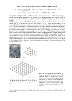


© Copyright 2026