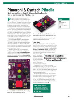
Python for High Performance Computing
Pawel Pomorski
SHARCNET
University of Waterloo
[email protected]
May 26,2015
Outline
◮
Speeding up Python code with NumPy
◮
Speeding up Python code with Cython
◮
Speeding up Python code via multiprocessing
◮
Using MPI with Python, via mpi4py
What is Python?
◮
Python is a programming language that appeared in 1991
◮
compare with Fortran (1957), C (1972), C++ (1983),
◮
While the older languages still dominate High Performance
Computing (HPC), popularity of Python is growing
Python advantages
◮
Designed from the start for better code readability
◮
Allows expression of concepts in fewer lines of code
◮
Has dynamic type system, variables do not have to be declared
◮
Has automatic memory management
◮
Has large number of easily accessible, extensive libraries (eg.
NumPy, SciPy)
◮
All this makes developing new codes easier
Python disadvantages
◮
Python is generally slower than compiled languages like C,
C++ and Fortran
◮
Complex technical causes include dynamic typing and the fact
that Python is interpreted, not compiled
◮
This does not matter much for a small desktop program that
runs quickly.
◮
However, this will matter a lot in a High Performance
Computing environment.
◮
Python use in HPC parallel environments is relatively recent,
hence parallel techniques less well known
◮
Rest of this talk will describe approaches to ensure your
Python code runs reasonably fast and in parallel
1D diffusion equation
To describe the dynamics of some quantity u(x,t) (eg. heat)
undergoing diffusion, use:
∂u
∂t
2
= κ ∂∂xu2
Problem: given some initial condition u(x,t=0), determine time
evolution of u and obtain u(x,t)
Use finite difference with Euler method for time evolution
u(i∆x,
h (m + 1)∆t) = u(i∆x, m∆t)+
i
κ∆t
u((i
+
1)∆x,
m∆t)
+
u((i
−
1)∆x,
m∆t)
−
2u(i∆x,
m∆t)
2
∆x
C code
1
2
#i n c l u d e <math . h>
#i n c l u d e <s t d i o . h>
3
4
i n t main ( ) {
5
6
i n t c o n s t n =100000 , n i t e r =500;
7
8
9
10
11
double
int i ,
double
double
x [ n ] , u [ n ] , udt [ n ] ;
iter ;
dx = 1 . 0 ;
kappa = 0 . 1 ;
12
13
14
15
16
f o r ( i =0; i <n ; i ++){
u [ i ]= exp (−pow ( dx ∗ ( i −n / 2 . 0 ) , 2 . 0 ) / 1 0 0 0 0 0 . 0 ) ;
udt [ i ] = 0 . 0 ;
}
17
18
...
C code continued :
1
2
3
4
5
6
7
8
9
10
11
...
f o r ( i t e r =0; i t e r <n i t e r ; i t e r ++){
f o r ( i =1; i <n −1; i ++){
u d t [ i ]=u [ i ]+ kappa ∗ ( u [ i +1]+u [ i −1]−2∗u [ i ] ) ;
}
f o r ( i =0; i <n ; i ++){
u [ i ]= u d t [ i ] ;
}
}
return 0;
}
Program output
1.0
0.8
0.6
0.4
0.2
0.0
48000
48500
49000
49500
50000
50500
51000
51500
52000
Figure: Evolution of u(x) after 50,000 time steps (blue line initial, red
line final)
NumPy
◮
To implement the same in Python, will need support for
efficient, large numerical arrays
◮
These provided by NumPy, an extension to Python
◮
NumPy (http://www.numpy.org/) along with SciPy
(http://www.scipy.org/) provide a large set of easily
accessible libraries which make Python so attractive to the
scientific community
”Vanilla” Python code
1
2
3
4
5
i m p o r t numpy a s np
n=100000 ; dx =1.0 ; n i t e r =500 ; kappa =0.1
x=np . a r a n g e ( n , d t y p e=” f l o a t 6 4 ” )
u=np . empty ( n , d t y p e=” f l o a t 6 4 ” )
u d t=np . empty ( n , d t y p e=” f l o a t 6 4 ” )
6
7
8
f o r i in xrange ( len (u) ) :
u [ i ]= np . exp ( −(dx ∗ ( i −n / 2 ) ) ∗ ∗ 2 / 1 0 0 0 0 0 )
9
10
udt [ : ] = 0 . 0
11
12
f o r i in xrange ( n i t e r ) :
13
14
15
f o r i i n x r a n g e ( 1 , n−1) :
u d t [ i ]=u [ i ]+ kappa ∗ ( u [ i +1]+u [ i −1]−2∗u [ i ] )
16
17
18
f o r i in xrange ( len (u) ) :
u [ i ]= u d t [ i ]
Vanilla code performance
◮
500 iterations, tested on Macbook Pro laptop (2011)
◮
C code compiled with GCC takes 0.21 seconds
◮
Python ”vanilla” code takes 64.75 seconds
◮
Python is much slower (by factor 308)
◮
Even though we are using Python arrays, code is slow because
loops are explicit
◮
Must use NumPy array operations instead
◮
The difficulty of eliminating loops varies.
Slicing NumPy arrays :
1
2
3
4
5
6
7
8
9
10
11
12
13
14
15
s h a r c n e t 1 : ˜ pawelpomorski$ python
Python 2 . 7 . 9 ( d e f a u l t , Dec 12 2 0 1 4 , 1 2 : 4 0 : 2 1 )
[ GCC 4 . 2 . 1 C o m p a t i b l e A p p l e LLVM 6 . 0 ( c l a n g − 6 0 0 . 0 . 5 6 ) ]
on d a r w i n
Type ” h e l p ” , ” c o p y r i g h t ” , ” c r e d i t s ” o r ” l i c e n s e ” f o r
more i n f o r m a t i o n .
>>> i m p o r t numpy a s np
>>> a=np . a r a n g e ( 1 0 )
>>> a
array ([0 , 1 , 2 , 3 , 4 , 5 , 6 , 7 , 8 , 9])
>>> a [ 1 : − 1 ]
array ([1 , 2 , 3 , 4 , 5 , 6 , 7 , 8])
>>> a [ 0 : − 2 ]
array ([0 , 1 , 2 , 3 , 4 , 5 , 6 , 7])
>>> a [1: −1]+ a [ 0 : − 2 ]
a r r a y ( [ 1 , 3 , 5 , 7 , 9 , 11 , 13 , 1 5 ] )
>>>
NumPy vector operations
Replace explicit loops
1
2
f o r i i n x r a n g e ( 1 , n−1) :
u d t [ i ]=u [ i ]+ kappa ∗ ( u [ i +1]+u [ i −1]−2∗u [ i ] )
with NumPy vector operations using slicing
1
u d t [1: −1]= u [1: −1]+ kappa ∗ ( u [0: −2]+ u [ 2 : ] − 2 ∗ u [ 1 : − 1 ] )
Python code using Numpy operations instead of loops
1
2
i m p o r t numpy a s np
3
4
n =100000; dx = 1 . 0 ; n i t e r =50000; kappa =0.1
5
6
7
8
x=np . a r a n g e ( n , d t y p e=” f l o a t 6 4 ” )
u=np . empty ( n , d t y p e=” f l o a t 6 4 ” )
u d t=np . empty ( n , d t y p e=” f l o a t 6 4 ” )
9
10
11
12
u i n i t = lambda x : np . exp ( −(dx ∗ ( x−n / 2 ) ) ∗ ∗ 2 / 1 0 0 0 0 0 )
u= u i n i t ( x )
udt [ : ] = 0 . 0
13
14
15
16
f o r i in xrange ( n i t e r ) :
u d t [1: −1]= u [1: −1]+ kappa ∗ ( u [0: −2]+ u [ 2 : ] − 2 ∗ u [ 1 : − 1 ] )
u [ : ] = udt [ : ]
Performance
◮
50,000 iterations, tested on Macbook Pro laptop (2011)
◮
C code compiled with gcc -O2 - 12.75 s
◮
C code compiled with gcc (unoptimized) - 34.31 s
◮
Python code with NumPy operations - 40.43 s
◮
Python 3.2 times slower than optimized code, only 1.2 times
slower than unoptimized code
◮
It’s likely that GCC can optimize the whole loop over
iterations, whereas Numpy vector operations optimize each
iteration individually
Numpy libraries
◮
For standard operations, eg. matrix multiply, will run at the
speed of underlying numerical library
◮
Performance will strongly depend on which library is used, can
see with numpy.show config()
◮
If libraries are threaded, python will take advantage of
multithreading, with no extra programming (free parallelism)
General approaches for code speedup
◮
NumPy does not help with all problems, some don’t fit array
operations
◮
Need a more general technique to speed up Python code
◮
As the problem is that Python is not a compiled language,
one can try to compile it
◮
General compiler: nuitka (http://nuitka.net/) under active
development
◮
PyPy (http://pypy.org/) - Just-in-Time (JIT) compiler
◮
Cython (http://cython.org)- turns Python program into C
and compiles it
Euler problem
If p is the perimeter of a right angle triangle with integral length
sides, a,b,c, there are exactly three solutions for p = 120.
(20,48,52), (24,45,51), (30,40,50)
For which value of p < N, is the number of solutions maximized?
Take N=1000 as starting point
(from https://projecteuler.net )
Get solutions at particular p
1
2
3
4
5
6
7
def find num solutions (p) :
n=0
f o r a i n range (1 , p /2) :
f o r b i n range ( a , p /2) :
c=p−a−b
i f ( a ∗ a+b∗b==c ∗ c ) :
n=n+1
8
9
return n
Loop over possible value of p up to N
1
2
nmax=0 ; imax=0
N=1000
3
4
5
6
7
8
f o r i i n r a n g e ( 1 ,N) :
print i
n s o l s=f i n d n u m s o l u t i o n s ( i )
i f ( n s o l s >nmax ) :
nmax=n s o l s ; imax=i
9
10
p r i n t ”maximum p , number o f s o l u t i o n s ” , imax , nmax
Cython
◮
The goal is to identify functions in the code where it spends
the most time. Python has profiler already built in
◮
python -m cProfile euler37.py
◮
Place those functions in a separate file so they are imported as
module
◮
Cython will take a python module file, convert it into C code,
and then compile it into a shared library
◮
Python will import that compiled library module at runtime
just like it would import a standard Python module
◮
To make Cython work well, need to provide some hints to the
compiler as to what the variables are, by defining some key
variables
Invoking Cython
1
2
◮
Place module code (with Cython modifications) in
find num solutions.pyx
◮
Create file setup.py
from d i s t u t i l s . c o r e i m p o r t s e t u p
from Cython . B u i l d i m p o r t c y t h o n i z e
3
4
5
6
setup (
e x t m o d u l e s=c y t h o n i z e ( ” f i n d n u m s o l u t i o n s . pyx ” ) ,
)
◮
Execute: python setup.py build ext –inplace
◮
Creates find num solutions.c, C code implementation of the
module
◮
From this creates find num solutions.so library which can be
imported as Python module at runtime
Get solutions at particular p, cythonized
1
2
3
4
5
6
7
8
def find num solutions ( int p) :
cdef int a , b , c , n
n=0
f o r a i n range (1 , p /2) :
f o r b i n range ( a , p /2) :
c=p−a−b
i f ( a ∗ a+b∗b==c ∗ c ) :
n=n+1
# note d e f i n i t i o n
# note d e f i n i t i o n
9
10
return n
This code in file find num solutions.pyx
Loop over possible value of p up to N, with Cython
Note changes at line 1 and line 9
1
import f i n d n u m s o l u t i o n s
2
3
nmax=0 ; imax=0 ; N=1000
4
5
6
7
8
9
f o r i i n r a n g e ( 1 ,N) :
print i
n s o l s=f i n d n u m s o l u t i o n s . f i n d n u m s o l u t i o n s ( i )
i f ( n s o l s >nmax ) :
nmax=n s o l s ; imax=i
10
11
p r i n t ”maximum p and , number o f s o l u t i o n s ” , imax , nmax
Speedup with Cython
For N=1000, tested on development node of orca cluster
◮
vanilla python : 14.158 s
◮
Cython without variable definitions : 8.87 s, speedup factor
1.6
◮
Cython with integer variables defined : 0.084 s, speedup
factor 168
ctypes - a foreign function library for Python
1
2
3
4
5
# compile C l i b r a r y with :
# g c c −s h a r e d −o l i b r a r y n a m e . s o
librarycode . c
import ctypes
l i b r a r y n a m e = c t y p e s . CDLL( ’ . / l i b r a r y n a m e . s o ’ )
l i b r a r y n a m e . s o m e f u n c t i o n ( argument1 )
Speedup with ctypes
For N=1000, tested on development node of orca cluster
◮
vanilla python : 14.158 s
◮
Cython without variable definitions : 8.87 s, speedup factor
1.6
◮
Cython with integer variables defined : 0.084 s, speedup
factor 168
◮
ctypes : 0.134, speedup factor 105, 1.6 times slower than
cython!
◮
pure C code (GCC): 0.134, same as ctypes (as expected)
◮
pure C code (icc): 0.0684 s (Intel compiler more efficient)
Parallelizing Python
◮
Once the serial version is optimized, need to parallelize
Python to do true HPC
◮
Threading approach does not work due to Global Interpreter
Lock
◮
In Python, you can have many threads, but only one executes
at any one time, hence no speedup
◮
Have to use multiple processes instead
Multiprocessing - apply
1
2
i m p o r t time , o s
from m u l t i p r o c e s s i n g i m p o r t P o o l
3
4
5
6
7
8
9
def f () :
s t a r t=t i m e . t i m e ( )
time . s l e e p (2)
end=t i m e . t i m e ( )
p r i n t ” i n s i d e f pid ” , os . g e t p i d ( )
r e t u r n end−s t a r t
10
11
12
13
p = P o o l ( p r o c e s s e s =1)
r e s u l t = p . apply ( f )
p r i n t ” apply i s blocking , t o t a l time ” , r e s u l t
14
15
16
r e s u l t =p . a p p l y a s y n c ( f )
p r i n t ” a p p l y a s y n c i s non−b l o c k i n g ”
17
18
19
20
w h i l e not r e s u l t . ready ( ) :
time . s l e e p ( 0 . 5 )
p r i n t ” c o u l d work h e r e w h i l e r e s u l t computes ”
21
22
p r i n t ” t o t a l time ” , r e s u l t . get ()
Multiprocessing - Map
1
2
import time
from m u l t i p r o c e s s i n g i m p o r t P o o l
3
4
5
def f ( x ) :
r e t u r n x ∗∗3
6
7
8
y = r a n g e ( i n t ( 1 e7 ) )
p= P o o l ( p r o c e s s e s =8)
9
10
11
12
s t a r t= t i m e . t i m e ( )
r e s u l t s = p . map ( f , y )
end = t i m e . t i m e ( )
13
14
p r i n t ”map b l o c k s on l a u n c h i n g p r o c e s s , t i m e=” , end−
start
15
16
17
18
19
20
21
22
# ma p a s y n c
s t a r t = time . time ()
r e s u l t s = p . ma p a s y n c ( f , y )
p r i n t ” ma p a s y n c i s non−b l o c k i n g on l a u n c h i n g p r o c e s s ”
output = r e s u l t s . get ()
end=t i m e . t i m e ( )
p r i n t ” t i m e ” , end−s t a r t
Euler problem with multiprocessing
1
2
from m u l t i p r o c e s s i n g i m p o r t P o o l
import f i n d n u m s o l u t i o n s
3
4
p= P o o l ( p r o c e s s e s =4)
5
6
7
8
y=r a n g e ( 1 , 1 0 0 0 )
r e s u l t s =p . map ( f i n d n u m s o l u t i o n s . f i n d n u m s o l u t i o n s , y )
p r i n t ” a n s w e r ” , y [ r e s u l t s . i n d e x ( max ( r e s u l t s ) ) ]
Multiprocessing performance
timing on orca development node (24 cores)
n=5000 case
Number of processes
1
2
4
8
16
24
time(s)
11.07
7.247
4.502
2.938
2.343
1.885
speedup
1.0
1.52
2.45
3.76
4.72
5.87
Will scale better for larger values of N (for example, for N=10000
get speedup 13.0 with 24 processors)
MPI - Message Passing Interface
◮
Approach has multiple processors with independent memory
running in parallel
◮
Since memory is not shared, data is exchanged via calls to
MPI routines
◮
Each process runs same code, but can identify itself in the
process set and execute code differently
Compare MPI in C and Python with mpi4py - MPI reduce
1
2
3
4
5
6
7
8
9
1
2
3
4
5
6
7
8
i n t main ( i n t a r g c , c h a r ∗ a r g v [ ] ) {
i n t my rank , imax , i m a x i n ;
M P I I n i t (& a r g c , &a r g v ) ;
MPI Comm rank (MPI COMM WORLD, &my rank ) ;
i m a x i n=my rank ;
MPI Reduce(& i m a x i n ,& imax , 1 , MPI INT , MPI MAX , 0 ,
MPI COMM WORLD) ;
i f ( my rank == 0 ) p r i n t f ( ”%d \n” , imax ) ;
MPI Finalize () ;
return 0;}
from mpi4py i m p o r t MPI
comm = MPI .COMM WORLD
myid = comm . G e t r a n k ( )
i m a x i n = myid
imax = comm . r e d u c e ( i m a x i n , op=MPI .MAX)
i f ( myid==0) :
p r i n t imax
MPI . F i n a l i z e
Loop over p values up to N distributed among MPI processes
1
2
from mpi4py i m p o r t MPI
import f i n d n u m s o l u t i o n s
3
4
5
6
comm = MPI .COMM WORLD
myid = comm . G e t r a n k ( )
n p r o c s = comm . G e t s i z e ( )
7
8
nmax=0 ; imax=0 ; N=5000
9
10
f o r i i n r a n g e ( 1 ,N) :
11
12
13
14
15
i f ( i%n p r o c s==myid ) :
n s o l s=f i n d n u m s o l u t i o n s . f i n d n u m s o l u t i o n s ( i )
i f ( n s o l s >nmax ) :
nmax=n s o l s ; imax=i
16
17
18
19
n m a x g l o b a l=comm . a l l r e d u c e ( nmax , op=MPI .MAX)
i f ( n m a x g l o b a l==nmax ) :
p r i n t ” p r o c e s s ” , myid , ” f o u n d maximum a t ” , imax
20
21
MPI . F i n a l i z e
MPI performance
timing on orca development node (24 cores)
n=5000 case
MPI processes
1
2
4
8
16
24
time(s)
10.254
6.597
4.015
2.932
2.545
2.818
speedup
1.0
1.55
2.55
3.49
4.02
3.64
Will scale better for larger values of N (for example, for N=10000
get speedup 13.4 with 24 processors)
Conclusion
◮
Python is generally slower than compiled languages like C
◮
With a bit of effort, can take a Python code which is a great
deal slower and make it only somewhat slower
◮
The tradeoff between slower code but faster development time
is something the programmer has to decide
◮
Tools currently under development should make this problem
less severe over time