
Introduction to Programming in Python: An
Introduction to Programming in Python This page intentionally left blank Introduction to Programming in Python An Interdisciplinary Approach Robert Sedgewick Kevin Wayne Robert Dondero Princeton University New York • Boston • Indianapolis • San Francisco Toronto • Montreal • London • Munich • Paris • Madrid Capetown • Sydney • Tokyo • Singapore • Mexico City Many of the designations used by manufacturers and sellers to distinguish their products are claimed as trademarks. Where those designations appear in this book, and the publisher was aware of a trademark claim, the designations have been printed with initial capital letters or in all capitals. The authors and publisher have taken care in the preparation of this book, but make no expressed or implied warranty of any kind and assume no responsibility for errors or omissions. No liability is assumed for incidental or consequential damages in connection with or arising out of the use of the information or programs contained herein. For information about buying this title in bulk quantities, or for special sales opportunities (which may include electronic versions; custom cover designs; and content particular to your business, training goals, marketing focus, or branding interests), please contact our corporate sales department at [email protected] or (800) 382-3419. For government sales inquiries, please contact [email protected]. For questions about sales outside the United States, please contact [email protected]. Visit us on the Web: informit.com/aw Library of Cataloging-in-Publication Data Sedgewick, Robert, 1946Introduction to programming in Python : an interdisciplinary approach / Robert Sedgewick, Kevin Wayne, Robert Dondero. pages cm Includes indexes. ISBN 978-0-13-407643-0 (hardcover : alk. paper)—ISBN 0-13-407643-5 1. Python (Computer program language) 2. Computer programming. I. Wayne, Kevin Daniel, 1971II. Dondero, Robert. III. Title. QA76.73.P98S43 2015 005.13'3—dc23 2015011936 Copyright © 2015 Pearson Education, Inc. All rights reserved. Printed in the United States of America. This publication is protected by copyright, and permission must be obtained from the publisher prior to any prohibited reproduction, storage in a retrieval system, or transmission in any form or by any means, electronic, mechanical, photocopying, recording, or likewise. To obtain permission to use material from this work, please submit a written request to Pearson Education, Inc., Permissions Department, 200 Old Tappan Road, Old Tappan, New Jersey 07675, or you may fax your request to 236-3290. ISBN-13: 978-0-13-407643-0 ISBN-10: 0-13-407643-5 Text printed in the United States on recycled paper at Edwards Brothers Malloy in Ann Arbor, Michigan. First printing, June 2015 ______________________________ To Adam, Andrew, Brett, Robbie, Henry, Iona, Rose, Peter, and especially Linda ______________________________ ______________________________ To Jackie and Alex ______________________________ ______________________________ To my family, especially Ellen and Meghan ______________________________ This page intentionally left blank Contents Preface . . . . . . . . . . . . . . . . . . . . xiii 1—Elements of Programming . . . . . . . . . . . . 1 1.1 Your First Program 2 1.2 Built-in Types of Data 14 1.3 Conditionals and Loops 56 1.4 Arrays 100 1.5 Input and Output 140 1.6 Case Study: Random Web Surfer 188 2—Functions and Modules . . . . . . . . . . . . 209 2.1 Defining Functions 210 2.2 Modules and Clients 248 2.3 Recursion 290 2.4 Case Study: Percolation 322 3—Object-Oriented Programming . . . . . . . . . 3.1 Using Data Types 352 3.2 Creating Data Types 402 3.3 Designing Data Types 450 3.4 Case Study: N-Body Simulation 496 351 4—Algorithms and Data Structures . . . . . . . . . 511 4.1 Performance 512 4.2 Sorting and Searching 556 4.3 Stacks and Queues 590 4.4 Symbol Tables 634 4.5 Case Study: Small-World Phenomenon 684 Context . . . . . . . . . . . . . . . . . . . 729 Glossary . . . . . . . . . . . . . . . . . . . 733 Index . . . . . . . . . . . . . . . . . . . . 739 This page intentionally left blank Programs Programsix Elements of Programming 1.1 Your First Program Program Program 1.2 Program Program Program Program Program Program Program Program Program Program Program Program Program Program Program 1.3.1 1.3.2 1.3.3 1.3.4 1.3.5 1.3.6 1.3.7 1.3.8 1.3.9 Flipping a fair coin . . . . . . . 59 Your first loop . . . . . . . . . 62 Computing powers of 2 . . . . . 64 Your first nested loops . . . . . 70 Harmonic numbers . . . . . . 73 Newton’s method . . . . . . . 75 Converting to binary. . . . . . . 77 Gambler’s ruin simulation . . . . 79 Factoring integers . . . . . . . 81 1.4.1 1.4.2 1.4.3 1.4.4 Program Program Program 2.2 Program Program Program Program Program Program Program Program Program 1.5.1 Generating a random sequence . 142 1.5.2 Interactive user input. . . . . . 150 1.5.3 Averaging a stream of numbers . 152 1.5.4 A simple filter. . . . . . . . . 156 1.5.5 Standard input to drawing filter .162 1.5.6 Function graph . . . . . . . . 164 1.5.7 Bouncing ball. . . . . . . . . 169 1.5.8 Digital signal processing . . . . 174 Case Study: Random Web Surfer Program Program Program Program Program Program Program 2.3 1.6.1 Computing the transition matrix. 191 1.6.2 Simulating a random surfer . . . 193 1.6.3 Mixing a Markov chain. . . . . 200 2.1.1 2.1.2 2.1.3 2.1.4 Harmonic numbers (revisited) . 213 Gaussian functions. . . . . . . 223 Coupon collector (revisited) . . . 225 Play that tune (revisited) . . . . 234 Modules and Clients Program 2.2.1 2.2.2 2.2.3 2.2.4 2.2.5 2.2.6 2.2.7 Gaussian functions module. . . . 250 Sample Gaussian client . . . . . 251 Random number module. . . . 261 Iterated function systems . . . . 269 Data analysis module . . . . . . 272 Plotting data values . . . . . . . 275 Bernoulli trials . . . . . . . . 277 Recursion Program Program Program Program Program 2.4 Sampling without replacement . 113 Coupon collector simulation . . . 117 Sieve of Eratosthenes. . . . . . 119 Self-avoiding random walks . . 128 Input and Output Program 1.6 String concatenation example . . . 23 Integer operators . . . . . . . . 26 Float operators . . . . . . . . 29 Quadratic formula. . . . . . . . 31 Leap year . . . . . . . . . . . 35 Arrays Program 1.5 1.2.1 1.2.2 1.2.3 1.2.4 1.2.5 Defining Functions Program Conditionals and Loops Program 1.4 1 1.1.1 Hello, World . . . . . . . . . . 4 1.1.2 Using a command-line argument . 7 Built-in Types of Data Program 1.3 Functions and Modules 2.3.1 2.3.2 2.3.3 2.3.4 2.3.5 Euclid’s algorithm . . . . . . . 295 Towers of Hanoi . . . . . . . . 298 Gray code . . . . . . . . . . . 303 Recursive graphics. . . . . . . 305 Brownian bridge. . . . . . . . 307 Case Study: Percolation Program Program Program Program Program Program Program 2.4.1 2.4.2 2.4.3 2.4.4 2.4.5 2.4.6 2.4.7 Percolation scaffolding . . . . . 326 Vertical percolation detection. . . 328 Percolation input/output . . . . 330 Visualization client . . . . . . . 331 Percolation probability estimate .333 Percolation detection . . . . . . 335 Adaptive plot client . . . . . . . 338 Object-Oriented Programming 3.1 Data Types Program Program Program Program Program Program Program Program Program Program Program 3.2 Creating Data Types Program Program Program Program Program Program Program Program 3.3 3.2.1 Charged particle . . . . . . . . 409 3.2.2 Stopwatch . . . . . . . . . . 413 3.2.3 Histogram . . . . . . . . . . 415 3.2.4 Turtle graphics . . . . . . . . 418 3.2.5 Spira mirabilis . . . . . . . . 421 3.2.6 Complex numbers. . . . . . . 427 3.2.7 Mandelbrot set . . . . . . . . 431 3.2.8 Stock account. . . . . . . . . 435 4.1 Program Program Program Program 3.3.1 Complex numbers (polar). . . . 456 3.3.2 Counter . . . . . . . . . . . 459 3.3.3 Spatial vectors . . . . . . . . . 466 3.3.4 Document sketch . . . . . . . 483 3.3.5 Similarity detection . . . . . . 485 Case Study: N-Body Simulation Program Program 3.4.1 Gravitational body . . . . . . . 500 3.4.2 N-body simulation. . . . . . . 503 Performance Program Program 4.2 Program Program Program Program Program Program 4.3 Program Program Program Program Program 4.3.1 4.3.2 4.3.3 4.3.4 4.3.5 4.3.6 Stack (resizing array) . . . . . . 594 Stack (linked list). . . . . . . . 598 Expression evaluation . . . . . . 605 FIFO queue (linked list) . . . . . 609 M/M/1 queue simulation . . . . 615 Load-balancing simulation . . . 618 Symbol Tables Program Program Program Program 4.5 4.2.1 Binary search (20 questions). . . 558 4.2.2 Bisection search . . . . . . . . 562 4.2.3 Binary search (in a sorted array) .565 4.2.4 Insertion sort . . . . . . . . . 569 4.2.5 Doubling test for sorts . . . . . 571 4.2.6 Mergesort . . . . . . . . . . . 574 4.2.7 Frequency counts . . . . . . . 579 Stacks and Queues Program 4.4 4.1.1 3-sum problem . . . . . . . . 515 4.1.2 Validating a doubling hypothesis .517 Sorting and Searching Program Designing Data Types Program 3.4 3.1.1 Identifying a potential gene . . . 359 3.1.2 Charged-particle client . . . . . 363 3.1.3 Albers squares . . . . . . . . . 368 3.1.4 Luminance module . . . . . . . 370 3.1.5 Converting color to grayscale. . . 374 3.1.6 Image scaling . . . . . . . . . 376 3.1.7 Fade effect . . . . . . . . . . 377 3.1.8 Visualizing electric potential . . . 379 3.1.9 Concatenating files. . . . . . . 383 3.1.10 Screen scraping for stock quotes .385 3.1.11 Splitting a file . . . . . . . . 387 Algorithms and Data Structures 4.4.1 Dictionary lookup. . . . . . . 641 4.4.2 Indexing . . . . . . . . . . 643 4.4.3 Hash table . . . . . . . . . . 649 4.4.4 Binary search tree . . . . . . . 656 Case Study: Small-World Phenomenon Program Program Program Program Program Program 4.5.1 4.5.2 4.5.3 4.5.4 4.5.5 4.5.6 Graph data type . . . . . . . . 691 Using a graph to invert an index .695 Shortest-paths client . . . . . . 699 Shortest-paths implementation .705 Small-world test. . . . . . . . 710 Performer–performer graph . . . 712 This page intentionally left blank This page intentionally left blank Preface T he basis for education in the last millennium was “reading, writing, and arithmetic”; now it is reading, writing, and computing. Learning to program is an essential part of the education of every student in the sciences and engineering. Beyond direct applications, it is the first step in understanding the nature of computer science’s undeniable impact on the modern world. This book aims to teach programming to those who need or want to learn it, in a scientific context. Our primary goal is to empower students by supplying the experience and basic tools necessary to use computation effectively. Our approach is to teach students that composing a program is a natural, satisfying, and creative experience. We progressively introduce essential concepts, embrace classic applications from applied mathematics and the sciences to illustrate the concepts, and provide opportunities for students to write programs to solve engaging problems. We use the Python programming language for all of the programs in this book—we refer to “Python” after “programming in the title to emphasize the idea that the book is about fundamental concepts in programming, not Python per se. This book teaches basic skills for computational problem solving that are applicable in many modern computing environments, and is a self-contained treatment intended for people with no previous experience in programming. This book is an interdisciplinary approach to the traditional CS1 curriculum, in that we highlight the role of computing in other disciplines, from materials science to genomics to astrophysics to network systems. This approach emphasizes for students the essential idea that mathematics, science, engineering, and computing are intertwined in the modern world. While it is a CS1 textbook designed for any first-year college student interested in mathematics, science, or engineering, the book also can be used for self-study or as a supplement in a course that integrates programming with another field. xiii Coverage The book is organized around four stages of learning to program: basic elements, functions, object-oriented programming, and algorithms . We provide the basic information readers need to build confidence in composing programs at each level before moving to the next level. An essential feature of our approach is to use example programs that solve intriguing problems, supported with exercises ranging from self-study drills to challenging problems that call for creative solutions. Basic elements include variables, assignment statements, built-in types of data, flow of control , arrays, and input/output, including graphics and sound. Functions and modules are the student’s first exposure to modular programming. We build upon familiarity with mathematical functions to introduce Python functions, and then consider the implications of programming with functions, including libraries of functions and recursion. We stress the fundamental idea of dividing a program into components that can be independently debugged, maintained, and reused. Object-oriented programming is our introduction to data abstraction. We emphasize the concepts of a data type and their implementation using Python’s class mechanism. We teach students how to use, create, and design data types. Modularity, encapsulation, and other modern programming paradigms are the central concepts of this stage. Algorithms and data structures combine these modern programming paradigms with classic methods of organizing and processing data that remain effective for modern applications. We provide an introduction to classical algorithms for sorting and searching as well as fundamental data structures and their application, emphasizing the use of the scientific method to understand performance characteristics of implementations. Applications in science and engineering are a key feature of the text. We motivate each programming concept that we address by examining its impact on specific applications. We draw examples from applied mathematics, the physical and biological sciences, and computer science itself, and include simulation of physical systems, numerical methods, data visualization, sound synthesis, image processing, financial simulation, and information technology. Specific examples include a treatment in the first chapter of Markov chains for web page ranks and case studies that address the percolation problem, n-body simulation, and the small-world phenomenon. These applications are an integral part of the text. They engage students in the material, illustrate the importance of the programming concepts, and xiv provide persuasive evidence of the critical role played by computation in modern science and engineering. Our primary goal is to teach the specific mechanisms and skills that are needed to develop effective solutions to any programming problem. We work with complete Python programs and encourage readers to use them. We focus on programming by individuals, not programming in the large. Use in the Curriculum This book is intended for a first-year college course aimed at teaching novices to program in the context of scientific applications. Taught from this book, prospective majors in any area of science and engineering will learn to program in a familiar context. Students completing a course based on this book will be well prepared to apply their skills in later courses in science and engineering and to recognize when further education in computer science might be beneficial. Prospective computer science majors, in particular, can benefit from learning to program in the context of scientific applications. A computer scientist needs the same basic background in the scientific method and the same exposure to the role of computation in science as does a biologist, an engineer, or a physicist. Indeed, our interdisciplinary approach enables colleges and universities to teach prospective computer science majors and prospective majors in other fields of science and engineering in the same course. We cover the material prescribed by CS1, but our focus on applications brings life to the concepts and motivates students to learn them. Our interdisciplinary approach exposes students to problems in many different disciplines, helping them to choose a major more wisely. Whatever the specific mechanism, the use of this book is best positioned early in the curriculum. First, this positioning allows us to leverage familiar material in high school mathematics and science. Second, students who learn to program early in their college curriculum will then be able to use computers more effectively when moving on to courses in their specialty. Like reading and writing, programming is certain to be an essential skill for any scientist or engineer. Students who have grasped the concepts in this book will continually develop that skill through a lifetime, reaping the benefits of exploiting computation to solve or to better understand the problems and projects that arise in their chosen field. xv Prerequisites This book is suitable for typical science and engineering students in their first year of college. That is, we do not expect preparation beyond what is typically required for other entry-level science and mathematics courses. Mathematical maturity is important. While we do not dwell on mathematical material, we do refer to the mathematics curriculum that students have taken in high school, including algebra, geometry, and trigonometry. Most students in our target audience automatically meet these requirements. Indeed, we take advantage of their familiarity with the basic curriculum to introduce basic programming concepts. Scientific curiosity is also an essential ingredient. Science and engineering students bring with them a sense of fascination with the ability of scientific inquiry to help explain what goes on in nature. We leverage this predilection with examples of simple programs that speak volumes about the natural world. We do not assume any specific knowledge beyond that provided by typical high school courses in mathematics, physics, biology, or chemistry. Programming experience is not necessary, but also is not harmful. Teaching programming is our primary goal, so we assume no prior programming experience. But composing a program to solve a new problem is a challenging intellectual task, so students who have written numerous programs in high school can benefit from taking an introductory programming course based on this book . The book can support teaching students with varying backgrounds because the applications appeal to both novices and experts alike. Experience using a computer is not necessary, but also is not at all a problem. College students use computers regularly, to communicate with friends and relatives, listen to music, to process photos, and as part of many other activities. The realization that they can harness the power of their own computer in interesting and important ways is an exciting and lasting lesson. In summary, virtually all students in science and engineering fields are prepared to take a course based on this book as a part of their first-semester curriculum. xvi Goals What can instructors of upper-level courses in science and engineering expect of students who have completed a course based on this book? We cover the CS1 curriculum, but anyone who has taught an introductory programming course knows that expectations of instructors in later courses are typically high: each instructor expects all students to be familiar with the computing environment and approach that he or she wants to use. A physics professor might expect some students to design a program over the weekend to run a simulation; an engineering professor might expect other students to be using a particular package to numerically solve differential equations; or a computer science professor might expect knowledge of the details of a particular programming environment. Is it realistic to meet such diverse expectations? Should there be a different introductory course for each set of students? Colleges and universities have been wrestling with such questions since computers came into widespread use in the latter part of the 20th century. Our answer to them is found in this common introductory treatment of programming, which is analogous to commonly accepted introductory courses in mathematics, physics, biology, and chemistry. An Introduction to Programming in Python strives to provide the basic preparation needed by all students in science and engineering, while sending the clear message that there is much more to understand about computer science than programming. Instructors teaching students who have studied from this book can expect that they will have the knowledge and experience necessary to enable those students to adapt to new computational environments and to effectively exploit computers in diverse applications. What can students who have completed a course based on this book expect to accomplish in later courses? Our message is that programming is not difficult to learn and that harnessing the power of the computer is rewarding. Students who master the material in this book are prepared to address computational challenges wherever they might appear later in their careers. They learn that modern programming environments, such as the one provided by Python, help open the door to any computational problem they might encounter later, and they gain the confidence to learn, evaluate, and use other computational tools. Students interested in computer science will be well prepared to pursue that interest; students in science and engineering will be ready to integrate computation into their studies. xvii Booksite An extensive amount of information that supplements this text may be found on the web at http://introcs.cs.princeton.edu/python For economy, we refer to this site as the booksite throughout. It contains material for instructors, students, and casual readers of the book. We briefly describe this material here, though, as all web users know, it is best surveyed by browsing. With a few exceptions to support testing, the material is all publicly available. One of the most important implications of the booksite is that it empowers instructors and students to use their own computers to teach and learn the material. Anyone with a computer and a browser can begin learning to program by following a few instructions on the booksite. The process is no more difficult than downloading a media player or a song. As with any website, our booksite is continually evolving. It is an essential resource for everyone who owns this book. In particular, the supplemental materials are critical to our goal of making computer science an integral component of the education of all scientists and engineers. For instructors, the booksite contains information about teaching. This information is primarily organized around a teaching style that we have developed over the past decade, where we offer two lectures per week to a large audience, supplemented by two class sessions per week where students meet in small groups with instructors or teaching assistants. The booksite has presentation slides for the lectures, which set the tone. For teaching assistants, the booksite contains detailed problem sets and programming projects, which are based on exercises from the book but contain much more detail. Each programming assignment is intended to teach a relevant concept in the context of an interesting application while presenting an inviting and engaging challenge to each student. The progression of assignments embodies our approach to teaching programming. The booksite fully specifies all the assignments and provides detailed, structured information to help students complete them in the allotted time, including descriptions of suggested approaches and outlines for what should be taught in class sessions. For students, the booksite contains quick access to much of the material in the book, including source code, plus extra material to encourage self-learning. Solutions are provided for many of the book’s exercises, including complete program code and test data. There is a wealth of information associated with programming assignments, including suggested approaches, checklists, FAQs, and test data. xviii For casual readers , the booksite is a resource for accessing all manner of extra information associated with the book’s content. All of the booksite content provides web links and other routes to pursue more information about the topic under consideration. There is far more information accessible than any individual could fully digest, but our goal is to provide enough to whet any reader’s appetite for more information about the book’s content. Acknowledgments This project has been under development since 1992, so far too many people have contributed to its success for us to acknowledge them all here. Special thanks are due to Anne Rogers, for helping to start the ball rolling; to Dave Hanson, Andrew Appel, and Chris van Wyk, for their patience in explaining data abstraction; and to Lisa Worthington, for being the first to truly relish the challenge of teaching this material to first-year students. We also gratefully acknowledge the efforts of /dev/126 ; the faculty, graduate students, and teaching staff who have dedicated themselves to teaching this material over the past 25 years here at Princeton University; and the thousands of undergraduates who have dedicated themselves to learning it. Robert Sedgewick Kevin Wayne Robert Dondero April 2015 xix Functions and Modules 2.1 Defining Functions You have been composing code that calls Python functions since the beginning of this book, from writing strings with stdio.writeln() to using type conversion functions such as str() and int() to computing mathematical functions such as math.sqrt() to using all of the functions in stdio, stddraw, and stdaudio. 2.1.1 Harmonic numbers (revisited). . . 213 In this section, you will learn how to de2.1.2 Gaussian functions . . . . . . . . . 223 fine and call your own functions. 2.1.3 Coupon collector (revisited) . . . . 225 2.1.4 Play that tune (revisited). . . . . . 234 In mathematics, a function maps an input value of one type (the domain) Programs in this section to an output value of another type (the range). For example, the square function f (x) = x 2 maps 2 to 4, 3 to 9, 4 to 16, and so forth. At first, we work with Python functions that implement mathematical functions, because they are so familiar. Many standard mathematical functions are implemented in Python’s math module, but scientists and engineers work with a broad variety of mathematical functions, which cannot all be included in the module. At the beginning of this section, you will learn how to implement and use such functions on your own. Later, you will learn that we can do more with Python functions than implement mathematical functions: Python functions can have strings and other types as their domain or range, and they can have side effects such as writing output. We also consider in this section how to use Python functions to organize programs and thereby simplify complicated programming tasks. From this point forward, we use the generic term function to mean either Python function or mathematical function depending on the context. We use the more specific terminology only when the context requires that we do so. Functions support a key concept that will pervade your approach to programming from this point forward: Whenever you can clearly separate tasks within a computation, you should do so. We will be overemphasizing this point throughout this section and reinforcing it throughout the rest of the chapter (and the rest of the book). When you write an essay, you break it up into paragraphs; when you compose a program, you break it up into functions. Separating a larger task into smaller ones is much more important when programming than when writing an essay, because it greatly facilitates debugging, maintenance, and reuse, which are all critical in developing good software. 2.1 Defining Functions Using and defining functions As you know from the functions you have been using, the effect of calling a Python function is easy to understand. For example, when you place math.sqrt(a-b) in a program, the effect is as if you had replaced that code with the return value that is produced by Python’s math.sqrt() function when passed the expression a-b as an argument. This usage is so intuitive that we have hardly needed to comment on it. If you think about what the system has to do to create this effect, however, you will see that it involves changing a program’s control flow. The implications of being able to change the control flow in this way are as profound as doing so for conditionals and loops. You can define functions in any Python program, using the def statement that specifies the function signature, followed by a sequence of statements that constitute the function. We will consider the details shortly, but begin with a simple example that illustrates how functions affect control flow. Our first example, Program 2.1.1 (harmonicf.py), includes a function named harmonic() that takes an argument n and computes the nth harmonic number (see Program 1.3.5). It also illustrates the typical structure of a Python program, having three components: • A sequence of import statements • A sequence of function definitions • Arbitrary global code, or the body of the program Program 2.1.1 has two import statements, one function definition, and four lines of arbitrary global code. Python executes the global code when we invoke the program by typing python harmonicf.py on the command line; that global code calls the harmonic() function defined earlier. The implementation in harmonicf.py is preferable to our original implementation for computing harmonic numbers (Program 1.3.5) because it clearly separates the two primary tasks performed by the program: calculating harmonic numbers and interacting with the user. (For purposes of illustration, we have made the user-interaction part of the program a bit more complicated than in Program 1.3.5.) Whenever you can clearly separate tasks within a computation, you should do so. Next, we carefully examine precisely how harmonicf.py achieves this goal. Control flow. The diagram on the next page illustrates the flow of control for the command python harmonicf.py 1 2 3. First, Python processes the import statements, thus making all of the features defined in the sys and stdio modules available to the program. Next, Python processes the definition of the harmonic() function at lines 4 through 8, but does not execute the function—Python executes 211 212 Functions and Modules a function only when it is called. Then, Python executes the first statement in the global code after the function definition, the for statement, which proceeds normally until Python begins to execute the statement value = harmonic(arg), starting by evaluating the expression harmonic(arg) when arg is 1. To do so it transfers control to the harmonic() function—the flow of control passes to the code in the funcimport sys tion definition. Python initialimport stdio izes the “parameter” variable n to 1 and the “local” varidef harmonic(n): able total to 0.0 and then executes the for loop within total = 0.0 harmonic(), which terminates for i in range(1, n+1): after one iteration with total total += 1.0 / i n=4 equal to 1.0. Then, Python return total n=2 1.0 executes the return statement n=1 1.5 2.08333... at the end of the definition of harmonic(), causing the flow of control to jump back for i in range(1, len(sys.argv)): to the calling statement vali=1 i=2 i=3 conue = harmonic(arg), arg = int(sys.argv[i]) tinuing from where it left off, but now with the expression harmonic(arg) replaced by value = harmonic(arg) 1.0. Thus, Python assigns 1.0 to value and writes it to stanstdio.writeln(value) dard output. Then, Python iterates the loop once more, and calls the harmonic() function a second time with n initialFlow of control for python harmonicf.py 1 2 4 ized to 2, which results in 1.5 being written. The process is then repeated a third time with arg (and then n) equal to 4, which results in 2.083333333333333 being written. Finally, the for loop terminates and the whole process is complete. As the diagram indicates, the simple code masks a rather intricate flow of control. 2.1 Defining Functions 213 Program 2.1.1 Harmonic numbers (revisited) (harmonicf.py) import sys import stdio def harmonic(n): total = 0.0 for i in range(1, n+1): total += 1.0 / i return total n parameter variable i loop index return value total for i in range(1, len(sys.argv)): arg = int(sys.argv[i]) value = harmonic(arg) stdio.writeln(value) i arg value argument index argument Harmonic number This program writes to standard output the harmonic numbers specified as command-line arguments. The program defines a function harmonic() that, given an int argument n, computes the nth harmonic number 1 + 1/2 + 1/3 + … + 1/n. % python harmonicf.py 1 2 4 1.0 1.5 2.083333333333333 % python harmonicf.py 10 100 1000 10000 2.9289682539682538 5.187377517639621 7.485470860550343 9.787606036044348 Abbreviation alert. We continue to use the abbreviations that we introduced in Section 1.2 for functions and function calls. For example, we might say, “The function call harmonic(2) returns the value 1.5,” instead of the more accurate but verbose “When we pass to harmonic() a reference to an object of type int whose value is 2, it returns a reference to an object of type float whose value is 1.5.” We strive to use language that is succinct and only as precise as necessary in a given context. Functions and Modules 214 Informal function call/return trace. One simple approach to following the control flow through function calls is to imagine that each function writes its name and argument(s) when it is called and its return value just before returning, with indentation added on calls and subi = 1 arg = 1 tracted on returns. The result enhances the process of tracharmonic(1) ing a program by writing the values of its variables, which total = 0.0 we have been using since Section 1.2. An informal trace for total = 1.0 return 1.0 our example is shown at right. The added indentation exvalue = 1.0 poses the flow of the control, and helps us check that each i = 2 function has the effect that we expect. Generally, adding calls arg = 2 on stdio.writef() to trace any program’s control flow in harmonic(2) total = 0.0 this way is a fine approach to begin to understand what it is total = 1.0 doing. If the return values match our expectations, we need total = 1.5 not trace the function code in detail, saving us a substantial return 1.5 value = 1.5 amount of work. i = 3 arg = 4 harmonic(4) total = 0.0 total = 1.0 total = 1.5 total = 1.8333333333333333 total = 2.083333333333333 return 2.083333333333333 value = 2.083333333333333 Informal trace with function call/return for python harmonicf.py 1 2 4 For the rest of this chapter, your programming will be centered on creating and using functions, so it is worthwhile to consider in more detail their basic properties and, in particular, the terminology surrounding functions. Following that, we will study several examples of function implementations and applications. Basic terminology. As we have been doing throughout, it is useful to draw a distinction between abstract concepts and Python mechanisms to implement them (the Python if statement implements the conditional, the while statement implements the loop, and so forth). There are several concepts rolled up in the idea of a mathematical function and there are Python constructs corresponding to each, as summarized in the table at the top of the following page. While you can rest assured that these formalisms have served mathematicians well for centuries (and have served programmers well for decades), we will refrain from considering in detail all of the implications of this correspondence and focus on those that will help you learn to program. When we use a symbolic name in a formula that defines a mathematical function (such as f (x) = 1 + x + x2), the symbol x is a placeholder for some input value 2.1 Defining Functions 215 concept Python construct description function function mapping input value argument input to function output value return value output of function formula function body function definition independent variable parameter variable symbolic placeholder for input value that will be substituted into the formula to determine the output value. In Python, we use a parameter variable as a symbolic placeholder and we refer to a particular input value where the function is to be evaluated as an argument. Function definition. The first line of a function signature function name parameter variable definition, known as its signature, gives a name to the function function and to each parameter variable. The signadef harmonic ( n ): body ture consists of the keyword def; the function name; a total= 0.0 local sequence of zero or more parameter variable names variable for i in range(1, n+1): separated by commas and enclosed in parentheses; total += 1.0 / i and a colon. The indented statements following the return total signature define the function body. The function body can consist of the kinds of statements that we return return statement value discussed in Chapter 1. It also can contain a return Anatomy of a function definition statement, which transfers control back to the point where the function was called and returns the result of the computation or return value. The body may also define local variables, which are variables that are available only inside the function in which they are defined. Function calls. As we have seen throughout, a Python function call is nothing more than the function name followed by its arguments, separated by commas and enclosed in parentheses, in precisely the same form as is customary for mathematical functions. As noted in Section 1.2, each argument can be an expression, which is for i in range(1, len(sys.argv)): evaluated and the resulting value passed as function arg = int(sys.argv[i]) call input to the function. When the function value = harmonic( arg ) finishes, the return value takes the place of stdio.writeln(value) argument the function call as if it were the value of a variable (perhaps within an expression). Anatomy of a function call Functions and Modules 216 Multiple arguments. Like a mathematical function, a Python function can have more than one parameter variable, so it can be called with more than one argument. The function signature lists the name of each parameter variable, separated by commas. For example, the following function computes the length of the hypotenuse of a right triangle with sides of length a and b: def hypot(a, b) return math.sqrt(a*a + b*b) Multiple functions. You can define as many functions as you want in a .py file. The functions are independent, except that they may refer to each other through calls. They can appear in any order in the file: def square(x): return x*x def hypot(a, b): return math.sqrt(square(a) + square(b)) However, the definition of a function must appear before any global code that calls it. That is the reason that a typical Python program contains (1) import statements, (2) function definitions, and (3) arbitrary global code, in that order. Multiple return statements. You can put return statements in a function wherever you need them: control goes back to the calling program as soon as the first statement is reached. This primality-testing function is an example of a function that is natural to define using multiple return statements: return def isPrime(n): if n < 2: return False i = 2 while i*i <= n: if n % i == 0: return False i += 1 return True Single return value. A Python function provides only one return value to the caller (or, more precisely, it returns a reference to one object). This policy is not as restrictive as it might seem, because Python data types can contain more informa- 2.1 Defining Functions 217 tion than a single number, boolean, or string. For example, you will see later in this section that you can use arrays as return values. Scope. The scope of a variable is the set of statements that can refer to that variable directly. The scope of a function’s local and parameter variables is limited to that function; the scope of a variable defined in global code—known as a global variable—is limited to the .py file containing that variable. Therefore, global code cannot refer to either a function’s local or parameter variables. Nor can one function refer to either the local or parameter variables that are defined in another function. When a function defines a local (or this code should not parameter) variable with the same name refer to arg or value as a global variable (such as i in Program 2.1.1), the variable name in the function def harmonic(n): total = 0.0 refers to the local (or parameter) variable, scope of for i in range(1, n+1): scope of i not the global variable. n and total total += 1.0 / i A guiding principle when designing return total two different variables software is to define each variable so that for i in range(1, len(sys.argv)): its scope is as small as possible. One of arg = int(sys.argv[i]) scope of i value = harmonic(arg) the important reasons that we use funcstdio.writeln(value) scope of tions is so that changes made to one part arg and value of a program will not affect an unrelated this code cannot refer to n or total part of the program. So, while code in Scope of local and parameter variables a function can refer to global variables, it should not do so: all communication from a caller to a function should take place via the function’s parameter variables, and all communication from a function to its caller should take place via the function’s return value. In Section 2.2, we consider a technique for removing most global code, thereby limiting scope and the potential for unexpected interactions. Default arguments. A Python function may designate an argument to be optional by specifying a default value for that argument. If you omit an optional argument in a function call, then Python substitutes the default value for that argument. We have already encountered a few examples of this feature. For example, math. log(x, b) returns the base-b logarithm of x. If you omit the second argument, then b defaults to math.e—that is, math.log(x) returns the natural logarithm of x. It might appear that the math module has two different logarithm functions, but it actually has just one, with an optional argument and a default value. Functions and Modules 218 You can specify an optional argument with a default value in a user-defined function by putting an equals sign followed by the default value after the parameter variable in the function signature. You can specify more than one optional argument in a function signature, but all of the optional arguments must follow all of the mandatory arguments. For example, consider the problem of computing the nth generalized harmonic number of order r : Hn, r = 1 + 1/2r + 1/3r + … + 1/nr . For example, H1, 2 = 1, H2, 2 = 5/4, and H2, 2 = 49/36. The generalized harmonic numbers are closely related to the Riemann zeta function from number theory. Note that the nth generalized harmonic number of order r = 1 is equal to the nth harmonic number. Therefore it is appropriate to use 1 as the default value for r if the caller omits the second argument. We specify by writing r=1 in the signature: def harmonic(n, r=1): total = 0.0 for i in range(1, n+1): total += 1.0 / (i ** r) return total With this definition, harmonic(2, 2) returns 1.25, while both harmonic(2, 1) and harmonic(2) return 1.5. To the client, it appears that we have two different functions, one with a single argument and one with two arguments, but we achieve this effect with a single implementation. Side effects. In mathematics, a function maps one or more input values to some output value. In computer programming, many functions fit that same model: they accept one or more arguments, and their only purpose is to return a value. A pure function is a function that, given the same arguments, always return the same value, without producing any observable side effects, such as consuming input, producing output, or otherwise changing the state of the system. So far, in this section we have considered only pure functions. However, in computer programming it is also useful to define functions that do produce side effects. In fact, we often define functions whose only purpose is to produce side effects. An explicit return statement is optional in such a function: control returns to the caller after Python executes the function’s last statement. Functions with no specified return value actually return the special value None, which is usually ignored. 2.1 Defining Functions 219 For example, the stdio.write() function has the side effect of writing the given argument to standard output (and has no specified return value). Similarly, the following function has the side effect of drawing a triangle to standard drawing (and has no specified return value): def drawTriangle(x0, stddraw.line(x0, stddraw.line(x1, stddraw.line(x2, y0, y0, y1, y2, x1, x1, x2, x0, y1, x2, y2): y1) y2) y0) It is generally poor style to compose a function that both produces side effects and returns a value. One notable exception arises in functions that read input. For example, the stdio.readInt() function both returns a value (an integer) and produces a side effect (consuming one integer from standard input). Type checking. In mathematics, the definition of a function specifies both the domain and the range. For example, for the harmonic numbers, the domain is the positive integers and the range is the positive real numbers. In Python, we do not specify the types of the parameter variables or the type of the return value. As long as Python can apply all of the operations within a function, Python executes the function and returns a value. If Python cannot apply an operation to a given object because it is of the wrong type, it raises a run-time error to indicate the invalid type. For example, if you call the square() function defined earlier with an int argument, the result is an int; if you call it with a float argument, the result is a float. However, if you call it with a string argument, then Python raises a TypeError at run time. This flexibility is a popular feature of Python (known as polymorphism) because it allows us to define a single function for use with objects of different types. It can also lead to unexpected errors when we call a function with arguments of unanticipated types. In principle, we could include code to check for such errors, and we could carefully specify which types of data each function is supposed to work with. Like most Python programmers, we refrain from doing so. However, in this book, our message is that you should always be aware of the type of your data, and the functions that we consider in this book are built in line with this philosophy, which admittedly clashes with Python’s tendency toward polymorphism. We will discuss this issue in some detail in Section 3.3. Functions and Modules 220 The table below summarizes our discussion by collecting together the function definitions that we have examined so far. To check your understanding, take the time to reread these examples carefully. def isPrime(n): if n < 2: return False i = 2 while i*i <= n: if n % i == 0: return False i += 1 return True primality test hypotenuse of a right triangle def hypot(a, b) return math.sqrt(a*a + b*b) generalized harmonic number def harmonic(n, r=1): total = 0.0 for i in range(1, n+1): total += 1.0 / (i ** r) return total draw a triangle def drawTriangle(x0, stddraw.line(x0, stddraw.line(x1, stddraw.line(x2, y0, y0, y1, y2, x1, x1, x2, x0, y1, x2, y2): y1) y2) y0) Typical code for implementing functions Implementing mathematical functions Why not just use the Python builtin functions and those that are defined in the standard or extension Python modules? For example, why not use the math.hypot() function instead of defining our own hypot() function? The answer to this question is that we do use such functions when they are present (because they are likely to be faster and more accurate). However, there is an unlimited number of functions that we may wish to use and only a finite number of functions is defined in the Python standard and extension modules. When you need a function that is not defined in the Python standard or extension modules, you need to define the function yourself. 2.1 Defining Functions 221 As an example, we consider the kind of code required for a familiar and important application that is of interest to many potential college students in the United States. In a recent year, over 1 million students took the Scholastic Aptitude Test (SAT). The test consists of two major sections: critical reading and mathematics. Scores range from 200 (lowest) to 800 (highest) on each section, so overall test scores range from 400 to 1600. Many universities consider these scores when making important decisions. For example, student athletes are required by the National Collegiate Athletic Association (NCAA), and thus by many universities, to have a combined score of at least 820 (out of 1600), and the minimum eligibility requirement for certain academic scholarships is 1500 (out of 1600). What percentage of test takers is ineligible for athletics? What percentage is eligible for the scholarships? Two functions from statistics enable us to compute accurate answers to these questions. The standard normal (Gaussian) probability 1 density function is characterized by the familiar bell-shaped distribution curve and defined by the formula (x) ex 2 2 2 . The standard normal (Gaussian) cumulative distribution function F(z) is defined to be the area under the curve (x) defined by f(x) above the x-axis and to the left of the area is (z0) vertical line x = z. These functions play an important role in science, engineering, and finance because they arise as 0 accurate models throughout the natural world and bez0 cause they are essential in understanding experimental 1 error. In particular, these functions are known to accurately describe the distribution of test scores in our ex- cumulative ample, as a function of the mean (average value of the scores) and the standard deviation (square root of the average of the squares of the differences between each (z0) score and the mean), which are published each year. Given the mean and the standard deviation of the test 0 z0 scores, the percentage of students with scores less than a given value z is closely approximated by the function Gaussian probability functions (z, , ) = ((z )/). Functions to calculate and are not available in Python’s math module, so we develop our own implementations. x z 222 Functions and Modules Closed form. In the simplest situation, we have a closed-form mathematical formula defining our function in terms of functions that are implemented in Python’s math module. This situation is the case for —the math module includes functions to compute the exponential and the square root functions (and a constant value for ), so a function pdf() corresponding to the mathematical definition is easy to implement. For convenience, gauss.py (Program 2.1.2) uses the default arguments = 0 and = 1 and actually computes (x, , ) = ((x ) / ) / . No closed form. If no formula is known, we may need a more complicated algorithm to compute function values. This situation is the case for —no closed-form expression exists for this function. Algorithms to compute function values sometimes follow immediately from Taylor series approximations, but developing reliably accurate implementations of mathematical functions is an art and a science that needs to be addressed carefully, taking advantage of the knowledge built up in mathematics over the past several centuries. Many different approaches have been studied for evaluating . For example, a Taylor series approximation to the ratio of and turns out to be an effective basis for evaluating the function: F(z) 12 f(z) ( z z 3 3 z 5 (35) z 7 (357) . . . ). This formula readily translates to the Python code for the function cdf() in Program 2.1.2. For small (respectively large) z, the value is extremely close to 0 (respectively 1), so the code directly returns 0 (respectively 1); otherwise, it uses the Taylor series to add terms until the sum converges. Again, for convenience, Program 2.1.2 actually computes (z, , ) = ((z ) / ), using the defaults = 0 and = 1. Running gauss.py with the appropriate arguments on the command line tells us that about 17% of the test takers were ineligible for athletics in a year when the mean was 1019 and the standard deviation was 209. In the same year, about 1% percent qualified for academic scholarships. Computing with mathematical functions of all sorts plays a central role in science and engineering. In a great many applications, the functions that you need are expressed in terms of the functions in Python’s math module, as we have just seen with pdf(), or in terms of a Taylor series approximation or some other formulation that is easy to compute, as we have just seen with cdf(). Indeed, support for such computations has played a central role throughout the evolution of computing systems and programming languages. 2.1 Defining Functions 223 Program 2.1.2 Gaussian functions (gauss.py) import math import sys import stdio def pdf(x, mu=0.0, sigma=1.0): x = float(x - mu) / sigma return math.exp(-x*x/2.0) / math.sqrt(2.0*math.pi) / sigma def cdf(z, mu=0.0, sigma=1.0): z = float(z - mu) / sigma if z < -8.0: return 0.0 if z > +8.0: return 1.0 total = 0.0 term = z i = 3 while total != total + term: total += term term *= z * z / i i += 2 return 0.5 + total * pdf(z) total term cumulated sum current term z = float(sys.argv[1]) mu = float(sys.argv[2]) sigma = float(sys.argv[3]) stdio.writeln(cdf(z, mu, sigma)) This code implements the Gaussian (normal) probability density (pdf) and cumulative distribution (cdf) functions, which are not implemented in Python’s math library. The pdf() implementation follows directly from its definition, and the cdf() implementation uses a Taylor series and also calls pdf() (see accompanying text at left and Exercise 1.3.36). Note: If you are referring to this code for use in another program, please see gaussian.py (Program 2.2.1), which is designed for reuse. % python gauss.py 820 1019 209 0.17050966869132106 % python gauss.py 1500 1019 209 0.9893164837383885 224 Functions and Modules Using functions to organize code Beyond evaluating mathematical functions, the process of calculating an output value as a function of input values is important as a general technique for organizing control flow in any computation. Doing so is a simple example of an extremely important principle that is a prime guiding force for any good programmer: Whenever you can clearly separate tasks within a computation, you should do so. Functions are natural and universal mechanism for expressing computational tasks. Indeed, the “bird’s-eye view” of a Python program that we began with in Section 1.1 was equivalent to a function: we began by thinking of a Python program as a function that transforms command-line arguments into an output string. This view expresses itself at many different levels of computation. In particular, it is generally the case that you can express a long program more naturally in terms of functions instead of as a sequence of Python assignment, conditional, and loop statements. With the ability to define functions, you can better organize your programs by defining functions within them when appropriate. For example, coupon.py (Program 2.1.3) on the facing page is an improved version of couponcollector.py (Program 1.4.2) that better separates the individual components of the computation. If you study Program 1.4.2, you will identify three separate tasks: • Given the number of coupon values n, compute a random coupon value. • Given n, do the coupon collection experiment. • Get n from the command line, then compute and write the result. Program 2.1.3 rearranges the code to reflect the reality that these three activities underlie the computation. The first two are implemented as functions, the third as global code. With this organization, we could change getCoupon() (for example, we might want to draw the random numbers from a different distribution) or the global code (for example, we might want to take multiple inputs or run multiple experiments) without worrying about the effect of any of these changes on collect(). Using functions isolates the implementation of each component of the collection experiment from others, or encapsulates them. Typically, programs have many independent components, which magnifies the benefits of separating them into different functions. We will discuss these benefits in further detail after we have seen several other examples, but you certainly can appreciate that it is better to express a computation in a program by breaking it up into functions, just as it is better to express an idea in an essay by breaking it up into paragraphs. Whenever you can clearly separate tasks within a computation, you should do so. 2.1 Defining Functions 225 Program 2.1.3 Coupon collector (revisited) (coupon.py) import import import import random sys stdarray stdio def getCoupon(n): return random.randrange(0, n) def collect(n): isCollected = stdarray.create1D(n, False) count = 0 n collectedCount = 0 isCollected[i] while collectedCount < n: count value = getCoupon(n) collectedCount count += 1 value if not isCollected[value]: collectedCount += 1 isCollected[value] = True return count # of coupon values (0 to n-1) has coupon i been collected? # of coupons collected # of distinct coupons collected value of current coupon n = int(sys.argv[1]) result = collect(n) stdio.writeln(result) This version of Program 1.4.2 illustrates the style of encapsulating computations in functions. This code has the same effect as couponcollector.py, but better separates the code into its three constituent pieces: generating a random integer between 0 and n-1, running a collection experiment, and managing the I/O. % python coupon.py 1000 6522 % python coupon.py 1000 6481 % python coupon.py 1000000 12783771 226 Functions and Modules Passing arguments and returning values Next, we examine the specifics of Python’s mechanisms for passing arguments to and returning values from functions. These mechanisms are conceptually very simple, but it is worthwhile to take the time to understand them fully, as the effects are actually profound. Understanding argument-passing and return-value mechanisms is key to learning any new programming language. In the case of Python, the concepts of immutability and aliasing play a central role. Call by object reference. You can use parameter variables anywhere in the body of the function in the same way as you use local variables. The only difference between a parameter variable and a local variable is that Python initializes the parameter variable with the corresponding argument provided by the calling code. We refer to this approach as call by object reference. (It is more commonly known as call by value, where the value is always an object reference—not the object’s value.) One consequence of this approach is that if a parameter variable refers to a mutable object and you change that object’s value within a function, then this also changes the object’s value in the calling code (because it is the same object). Next, we explore the ramifications of this approach. Immutability and aliasing. As discussed in Section 1.4, arrays are mutable data types, because we can change array elements. By contrast, a data type is immutable if it is not possible to change the value of an object of that type. The other data types that we have been us- informal trace i j i = 99 99 ing (int, float, str, and bool) are all immutable. In j = i 99 99 an immutable data type, operations that might seem j += 1 99 100 to change a value actually result in the creation of a new object, as illustrated in the simple example at object-level trace right. First, the statement i = 99 creates an integer i i = 99 99 99, and assigns to i a reference to that integer. Then j = i j j = i assigns i (an object reference) to j, so both i i 99 and j reference the same object—the integer 99. Two variables that reference the same objects are said to j += 1 100 be aliases. Next, j += 1 results in j referencing an j 1 object with value 100, but it does not do so by changi 99 ing the value of the existing integer from 99 to 100! Indeed, since int objects are immutable, no statement Immutability of integers 2.1 Defining Functions 227 can change the value of that existing integer. Instead, that statement creates a new integer 1, adds it to the integer 99 to create another new integer 100, and assigns to j a reference to that integer. But i still references the original 99. Note that the new integer 1 has no reference to it in the end—that is the system’s concern, not ours. The immutability of integers, floats, strings, and booleans is a fundamental aspect of Python. We will consider the advantages and disadvantages of this approach in more detail in Section 3.3. Integers, floats, booleans, and strings as arguments. The key point to remember about passing arguments to functions in Python is that whenever you pass arguments to a function, the arguments and the function’s parameter variables become aliases. In practice, this is the predominant use of aliasing in Python, and it is important to understand its effects. For purposes of illustration, suppose that we need a function that increments an integer (our discussion applies to any more complicated function as well). A programmer new to Python might try this definition: def inc(j): j += 1 informal trace i = 99 inc(i) j += 1 i 99 99 99 99 j and then expect to increment an integer i with the call 99 Code like this would work in some program100 (after return) ming languages, but it has no effect in Python, as shown 100 in the figure at right. First, the statement i = 99 assigns to global variable i a reference to the integer 99. Then, object-level trace i i = 99 the statement inc(i) passes i, an object reference, to 99 the inc() function. That object reference is assigned inc(i) j to the parameter variable j. At this point i and j are i 99 aliases. As before, the inc() function’s j += 1 statement does not change the integer 99, but rather creates j += 1 100 a new integer 100 and assigns a reference to that integer j 1 to j. But when the inc() function returns to its caller, i 99 its parameter variable j goes out of scope, and the variable i still references the integer 99. (after return) 100 This example illustrates that, in Python, a function 1 cannot produce the side effect of changing the value of an i 99 integer object (nothing can do so). To increment variable i, we could use the definition Aliasing in a function call inc(i). Functions and Modules 228 def inc(j): j += 1 return j and call the function with the assignment statement i = inc(i). The same holds true for any immutable type. A function cannot change the value of an integer, a float, a boolean, or a string. Arrays as arguments. When a function takes an array as an argument, it implements a function that operates on an arbitrary number of objects. For example, the following function computes the mean (average) of an array of floats or integers: def mean(a): total = 0.0 for v in a: total += v return total / len(a) We have been using arrays as arguments from the beginning of the book. For example, by convention, Python collects the strings that you type after the program name in the python command into an array sys.argv[] and implicitly calls your global code with that array of strings as the argument. Side effects with arrays. Since arrays are mutable, it is often the case that the purpose of a function that takes an array as argument is to produce a side effect (such as changing the order of array elements). A prototypical example of such a function is one that exchanges the elements at two given indices in a given array. We can adapt the code that we examined at the beginning of Section 1.4: def exchange(a, i, j): temp = a[i] a[i] = a[j] a[j] = temp This implementation stems naturally from the Python array representation. The first parameter variable in exchange() is a reference to the array, not to all of the array’s elements: when you pass an array as an argument to a function, you are giving it the opportunity to operate on that array (not a copy of it). A formal trace of a call on this function is shown on the facing page. This diagram is worthy of careful study to check your understanding of Python’s function-call mechanism. 2.1 Defining Functions 229 A second prototypical example of a function that takes an array argument and produces side effects is one that randomly shuffles the elements in the array, using this version of the algorithm that we examined in Section 1.4 (and the exchange() function just defined): def shuffle(a): n = len(a) for i in range(n): r = random.randrange(i, n) exchange(a, i, r) Incidentally, Python’s standard function random.shuffle() does the same task. As another example, we will consider in Section 4.2 functions that sort an array (rearrange its elements so that they are in order). x = [.30, .60, .10] Arrays as return values. A function that sorts, shuffles, or otherwise modifies an array taken as argument does not have to return a reference to that array, because it is changing the contents of a client array, not a copy. But there are many situations where it is useful for a function to provide an array as a return value. Chief among these are functions that create arrays for the purpose of returning multiple objects of the same type to a client. As an example, consider the following function, which returns an array of random floats: def randomarray(n): a = stdarray.create1D(n) for i in range(n): a[i] = random.random() return a Later in this chapter, we will be developing numerous functions that return huge amounts of data in this way. x .30 0 1 2 .60 .10 3 exchange(x, 0, 2) 2 j 0 i a x .30 0 1 2 .60 .10 3 temp = a[i] a[i] = a[j] a[j] = temp temp 2 j 0 i a x .30 0 1 2 .60 3 (after return) x .10 .30 0 1 2 .60 3 .10 Exchanging two elements in an array Functions and Modules 230 The table below concludes our discussion of arrays as function arguments by highlighting some typical array-procession functions. def mean(a): total = 0.0 for v in a: total += v return total / len(a) mean of an array dot product of two vectors of the same length exchange two elements in an array write a one-dimensional array (and its length) read a two-dimensional array of floats (with dimensions) def dot(a, b): total = 0 for i in range(len(a)): total += a[i] * b[i] return total def exchange(a, i, j): temp = a[i] a[i] = a[j] a[j] = temp def write1D(a): stdio.writeln(len(a)) for v in a: stdio.writeln(v) def readFloat2D(): m = stdio.readInt() n = stdio.readInt() a = stdarray.create2D(m, n, 0.0) for i in range(m): for j in range(n): a[i][j] = stdio.readFloat() return a Typical code for implementing functions with arrays 2.1 Defining Functions Example: superposition of sound waves As discussed in Section 1.5, the simple audio model that we studied there needs to be embellished to create sound that resembles the sound produced by a musical instrument. Many different embellishments are possible; with functions, we can systematically apply them to produce sound waves that are far more complicated than the simple sine waves that we produced in Section 1.5. As an illustration of the effective use of functions to solve an interesting computational problem, we consider a program that has essentially the same functionality as playthattune.py (Program 1.5.8), but adds harmonic tones one octave above and one octave below each note to produce a more realistic sound. Chords and harmonics. Notes like concert A have a pure sound that is not very musical, because the sounds that you are accustomed to hearing have many other components. The sound from a guitar A 440.00 string echoes off the wooden part of the C♯ 554.37 instrument, the walls of the room that E 659.26 you are in, and so forth. You may think A major chord of such effects as modifying the basic sine wave. For example, most musical instruments produce harmonics (the same A 440.00 note in different octaves and not as loud), A 220.00 A 880.00 or you might play chords (multiple notes at the same time). To combine multiple concert A with harmonics sounds, we use superposition: simply add their waves together and rescale to Superposing waves to make composite sounds make sure that all values stay between 1 and 1. As it turns out, when we superpose sine waves of different frequencies in this way, we can get arbitrarily complicated waves. Indeed, one of the triumphs of 19th-century mathematics was the development of the idea that any smooth periodic function can be expressed as a sum of sine and cosine waves, known as a Fourier series. This mathematical idea corresponds to the notion that we can create a large range of sounds with musical instruments or our vocal cords and that all sound consists of a composition of various oscillating curves. Any sound corresponds to a curve and any curve corresponds to a sound, so we can create arbitrarily complex curves with superposition. 231 232 Functions and Modules Computing with sound waves. In Section 1.5, we saw how to represent sound waves by arrays of numbers that represent their values at the same sample points. Now, we will use such arrays as return values and arguments to functions to process such data. For example, the following function takes a frequency (in hertz) and a duration (in seconds) as arguments and returns a representation of a sound wave (more precisely, an array that contains values sampled from the specified wave at the standard 44,100 samples per second). def tone(hz, duration, sps=44100): n = int(sps * duration) a = stdarray.create1D(n+1, 0.0) for i in range(n+1): a[i] = math.sin(2.0 * math.pi * i * hz / sps) return a The size of the array returned depends on the duration: it contains about sps*duration floats (nearly half a million floats for 10 seconds). But we can now treat that array (the value returned from tone) as a single entity and compose code that processes sound waves, as we will soon see in Program 2.1.4. Weighted superposition. Since we represent sound waves by arrays of numbers that represent their values at the same sample points, superposition is simple to implement: we add together their sample values at each sample point to produce the combined result. For greater control, we also specify a relative weight for each of the two waves to be superposed, with the following function: def superpose(a, b, aWeight, bWeight): c = stdarray.create1D(len(a), 0.0) for i in range(len(a)): c[i] = aWeight*a[i] + bWeight*b[i] return c (This code assumes that a[] and b[] are of the same length.) For example, if we have a sound represented by an array a[] that we want to have three times the effect of the sound represented by an array b[], we would call superpose(a, b, 0.75, 0.25). The figure at the top of the next page shows the use of two calls on this function to add harmonics to a tone (we superpose the harmonics, then superpose the result with the original tone, which has the effect of giving the original tone twice 2.1 Defining Functions 233 0.982 lo = tone(220, 1.0/220.0) lo[44] = 0.982 hi = tone(880, 1.0/220.0) hi[44] = -0.693 -0.693 harmonics = superpose(lo, hi, 0.5, 0.5) harmonics[44] = 0.5*lo[44] + 0.5*hi[44] = 0.5*0.982 + 0.5*0.693 = 0.144 0.144 concertA = tone(440, 1.0/220.0) 0.374 concertA[44] = 0.374 superpose(harmonics, concertA, 0.5, 0.5) 0.259 0.5*harmonics[44] + 0.5*concertA[44]) = 0.5*.144 + 0.5*0.374 = 0.259 44 Adding harmonics to concert A (1/220 second at 44,100 samples/second) the weight of each harmonic). As long as the weights are positive and sum to 1, keeping the values of all waves between 1 and 1. superpose() preserves our convention of Program 2.1.4 (playthattunedeluxe.py) is an implementation that applies these concepts to produce a more realistic sound than that produced by Program 1.5.8. To do so, it makes use of functions to divide the computation into four parts: • Given a frequency and duration, create a pure tone. • Given two sound waves and relative weights, superpose them. • Given a pitch and duration, create a note with harmonics. • Read and play a sequence of pitch/duration pairs from standard input. Functions and Modules 234 Program 2.1.4 Play that tune (revisited) (playthattunedeluxe.py) import import import import math stdarray stdaudio stdio def superpose(a, b, aWeight, bWeight): c = stdarray.create1D(len(a), 0.0) for i in range(len(a)): c[i] = aWeight*a[i] + bWeight*b[i] return c def tone(hz, duration, sps=44100): n = int(sps * duration) a = stdarray.create1D(n+1, 0.0) for i in range(n+1): a[i] = math.sin(2.0 * math.pi * i * hz / sps) return a def note(pitch, duration): hz = 440.0 * (2.0 ** (pitch / 12.0)) lo = tone(hz/2, duration) hi = tone(2*hz, duration) harmonics = superpose(lo, hi, 0.5, 0.5) a = tone(hz, duration) return superpose(harmonics, a, 0.5, 0.5) hz lo[] frequency lower harmonic hi[] upper harmonic h[] combined harmonics a[] pure tone while not stdio.isEmpty(): pitch = stdio.readInt() duration = stdio.readFloat() a = note(pitch, duration) stdaudio.playSamples(a) stdaudio.wait() This program reads sound samples, embellishes the sounds by adding harmonics to create a more realistic tone than Program 1.5.8, and plays the resulting sound to standard audio. % python playthattunedeluxe.py < elise.txt % 7 7 2 0 more elise.txt .125 6 .125 .125 6 .125 7 .125 .125 5 .125 3 .125 .25 2.1 Defining Functions These tasks are all amenable to implementation as functions, which depend on one another. Each function is well defined and straightforward to implement. All of them (and stdaudio) represent sound as a series of discrete values kept in an array, corresponding to sampling a sound wave at 44,100 samples per second. Up to this point, our use of functions has been somewhat of a notational convenience. For example, the control flow in Program 2.1.1, Program 2.1.2, and Program 2.1.3 is simple—each function is called in just one place in the code. By contrast, Program 2.1.4 is a convincing example of the effectiveness of defining functions to organize a computation because each function is called multiple times. For example, as illustrated in the figure below, the function note() calls the function tone() three times and the function superpose() twice. Without functions, we would need multiple copies of the code in tone() and superpose(); with functions, we can deal directly with concepts close to the application. Like loops, functions have a simple but profound effect: one sequence of statements (those in the function definition) is executed multiple times during the execution of our program—once for each time the function is called in the control flow in the global code. 235 import import import import math stdarray stdaudio stdio def superpose(a, b, aWeight, bWeight): c = stdarray.create1D(len(a), 0.0) for i in range(len(a)): c[i] = aWeight*a[i] + bWeight*b[i] return c def tone(hz, duration, sps=44100): n = int(sps * duration) a = stdarray.create1D(n+1, 0.0) for i in range(n+1): a[i] = math.sin(2 * math.pi * i * hz / sps) return a def note(pitch, duration): hz = 440.0 * (2.0 ** (pitch / 12.0)) lo = tone(hz/2, duration) hi = tone(2*hz, duration) harmonics = superpose(lo, hi, 0.5, 0.5) a = tone(hz, duration) return superpose(harmonics, a, 0.5, 0.5) while not stdio.isEmpty(): pitch = stdio.readInt() duration = stdio.readFloat() a = note(pitch, duration) stdaudio.playArray(a) stdaudio.wait() Flow of control among several functions 236 Functions and Modules Functions are important because they give us the ability to extend the Python language within a program. Having implemented and debugged functions such as harmonic(), pdf(), cdf(), mean(), exchange(), shuffle(), isPrime(), superpose(), tone(), and note(), we can use them almost as if they were built into Python. The flexibility to do so opens up a whole new world of programming. Before, you were safe in thinking about a Python program as a sequence of statements. Now you need to think of a Python program as a set of functions that can call one another. The statement-to-statement control flow to which you have been accustomed is still present within functions, but programs have a higher-level control flow defined by function calls and returns. This ability enables you to think in terms of operations called for by the application, not just the operations that are built into Python. Whenever you can clearly separate tasks within a computation, you should do so. The examples in this section (and the programs throughout the rest of the book) clearly illustrate the benefits of adhering to this maxim. With functions, we can • Divide a long sequence of statements into independent parts. • Reuse code without having to copy it. • Work with higher-level concepts (such as sound waves). This point of view leads to code that is easier to understand, maintain, and debug compared to a long program composed solely of Python assignment, conditional, and loop statements. In the next section, we discuss the idea of using functions defined in other files, which again takes us to another level of programming. 2.1 Defining Functions Q&A Q. Can I use the statement return in a function without specifying a value? A. Yes. Technically, it returns the None object, which is the sole value of the type NoneType. Q. What happens if a function has one control flow that leads to a return statement that returns a value but another control flow that reaches the end of the function body? A. It would be poor style to define such a function, because doing so would place a severe burden on the function’s callers: the callers would need to know under which circumstances the function returns a value, and under which circumstances it returns None. Q. What happens if I compose code in the body of a function that appears after the return statement? A. Once a return statement is reached, control returns to the caller. So any code in the body of a function that appears after a return statement is useless; it is never executed. In Python, it is poor style, but not illegal to define such a function. Q. What happens if I define two functions with the same name (but possibly a different number of arguments) in the same .py file? A. This is known as function overloading, which is embraced by many programming languages. Python, however, is not one of those languages: the second function definition will overwrite the first one. You can often achieve the same effect by using default arguments. Q. What happens if I define two functions with the same name in different files? A. That is fine. For example, it would be good design to have a function named in gauss.py that computes the Gaussian probability density function and another function named pdf() in cauchy.py that computes the Cauchy probability density function. In Section 2.2 you will learn how to call functions defined in different .py files. pdf() Q. Can a function change the object to which a parameter variable is bound? 237 Functions and Modules 238 A. Yes, you can use a parameter variable on the left side of an assignment statement. However, many Python programmers consider it poor style to do so. Note that such an assignment statement has no effect in the client. Q. The issue with side effects and mutable objects is complicated. Is it really all that important? A. Yes. Properly controlling side effects is one of a programmer’s most important tasks in large systems. Taking the time to be sure that you understand the difference between passing arrays (which are mutable) and passing integers, floats, booleans, and strings (which are immutable) will certainly be worthwhile. The very same mechanisms are used for all other types of data, as you will learn in Chapter 3. Q. How can I arrange to pass an array to a function in such a way that the function cannot change the elements in the array? A. There is no direct way to do so. In Section 3.3 you will see how to achieve the same effect by building a wrapper data type and passing an object of that type instead. You will also see how to use Python’s built-in tuple data type, which represents an immutable sequence of objects. Q. Can I use a mutable object as a default value for an optional argument? A. Yes, but it may lead to unexpected behavior. Python evaluates a default value only once, when the function is defined (not each time the function is called). So, if the body of a function modifies a default value, subsequent function calls will use the modified value. Similar difficulties arise if you initialize the default value by calling an impure function. For example, after Python executes the code fragment def append(a=[], x=random.random()): a += [x] return a b = append() c = append() b[] and c[] are aliases for the same array of length 2 (not 1), which contains one float repeated twice (instead of two different floats). 2.1 Defining Functions 239 Exercises 2.1.1 Compose a function max3() that takes three int or float arguments and returns the largest one. 2.1.2 Compose a function that takes three bool arguments and returns True if an odd number of arguments are True, and False otherwise. odd() 2.1.3 Compose a function majority() that takes three bool arguments and returns True if at least two of the arguments are True, and False otherwise. Do not use an if statement. 2.1.4 Compose a function areTriangular() that takes three numbers as arguments and returns True if they could be lengths of the sides of a triangle (none of them is greater than or equal to the sum of the other two), and False otherwise. 2.1.5 Compose a function sigmoid() that takes a float argument x and returns the float obtained from the formula 1 (1+ex). 2.1.6 Compose a function lg() that takes an integer n as an argument and returns the base-2 logarithm of n. You may use Python’s math module. 2.1.7 Compose a function lg() that takes an integer n as an argument and returns the largest integer not larger than the base-2 logarithm of n. Do not use the math module. 2.1.8 Compose a function signum() that takes a float argument n -1 if n is less than 0, 0 if n is equal to 0, and +1 if n is greater than 0. 2.1.9 Consider this function duplicate(): def duplicate(s): t = s + s What does the following code fragment write? s = 'Hello' s = duplicate(s) t = 'Bye' t = duplicate(duplicate(duplicate(t))) stdio.writeln(s + t) and returns Functions and Modules 240 2.1.10 Consider this function cube(): def cube(i): i = i * i * i How many times is the following while loop iterated? i = 0 while i < 1000: cube(i) i += 1 Solution: Just 1,000 times. A call to cube() has no effect on the client code. It changes the parameter variable i, but that change has no effect on the variable i in the while loop, which is a different variable. If you replace the call to cube(i) with the statement i = i * i * i (maybe that was what you were thinking), then the loop is iterated five times, with i taking on the values 0, 1, 2, 9, and 730 at the beginning of the five iterations. 2.1.11 What does the following code fragment write? for i in range(5): stdio.write(i) for j in range(5): stdio.write(i) Solution: 0123444444. Note that the second call to stdio.write() uses i, not j. Unlike analogous loops in many other programming languages, when the first for loop terminates, the variable i is 4 and it remains in scope. 2.1.12 The following checksum formula is widely used by banks and credit card companies to validate legal account numbers: d0 f (d1) d2 f (d3) d4 f (d5) . . . = 0 (mod 10) The di are the decimal digits of the account number and f (d) is the sum of the decimal digits of 2d (for example, f (7) = 5 because 2 7 = 14 and 1 4 = 5). For example 17327 is valid because 1 + 5 + 3 + 4 + 7 = 20, which is a multiple of 10. 2.1 Defining Functions Implement the function f and compose a program to take a 10-digit integer as a command-line argument and write a valid 11-digit number with the given integer as its first 10 digits and the checksum as the last digit. 2.1.13 Given two stars with angles of declination and right ascension (d1, a1) and (d2, a2), respectively, the angle they subtend is given by the formula 2 arcsin((sin2(d/2) + cos (d1)cos(d2)sin2(a/2))1/2), where a1 and a2 are angles between 180 and 180 degrees, d1 and d2 are angles between 90 and 90 degrees, a = a2 a1, and d = d2 d1. Compose a program to take the declination and right ascension of two stars as command-line arguments and write the angle they subtend. Hint : Be careful about converting from degrees to radians. 2.1.14 Compose a readBool2D() function that reads a two-dimensional matrix of 0 and 1 values (with dimensions) into an array of booleans. Solution : The body of the function is virtually the same as for the corresponding function given in the table in the text for two-dimensional arrays of floats: def readBool2D(): m = stdio.readInt() n = stdio.readInt() a = stdarray.create2D(m, n, False) for i in range(m): for j in range(n): a[i][j] = stdio.readBool() return a 2.1.15 Compose a function that takes an array a[] of strictly positive floats as its argument and rescales the array so that each element is between 0 and 1 (by subtracting the minimum value from each element and then dividing each element by the difference between the minimum and maximum values). Use the built-in max() and min() functions. 241 Functions and Modules 242 2.1.16 Compose a function histogram() that takes an array a[] of integers and an integer m as arguments and returns an array of length m whose ith element is the number of times the integer i appears in the argument array. Assume that the values in a[] are all between 0 and m-1, so that the sum of the values in the returned array should be equal to len(a). 2.1.17 Assemble code fragments in this section and in Section 1.4 to develop a program that takes an integer n from the command line and writes n five-card hands, separated by blank lines, drawn from a randomly shuffled card deck, one card per line using card names like Ace of Clubs. 2.1.18 Compose a function multiply() that takes two square matrices of the same dimension as arguments and returns their product (another square matrix of that same dimension). Extra credit : Make your program work whenever the number of columns in the first matrix is equal to the number of rows in the second matrix. 2.1.19 Compose a function any() that takes an array of booleans as an argument and returns True if any of the elements in the array is True, and False otherwise. Compose a function all() that takes an array of booleans as an argument and returns True if all of the elements in the array are True, and False otherwise. Note that all() and any() are built-in Python functions; the goal of this exercise is to understand them better by creating your own versions. 2.1.20 Develop a version of getCoupon() that better models the situation when one of the n coupons is rare: choose one value at random, return that value with probability 1/(1000n), and return all other values with equal probability. Extra credit: How does this change affect the average value of the coupon collector function? 2.1.21 Modify playthattune.py to add harmonics two octaves away from each note, with half the weight of the one-octave harmonics. 2.1 Defining Functions Creative Exercises 2.1.22 Birthday problem. Compose a program with appropriate functions for studying the birthday problem (see Exercise 1.4.35). 2.1.23 Euler’s totient function. Euler’s totient function is an important function in number theory: (n) is defined as the number of positive integers less than or equal to n that are relatively prime with n (no factors in common with n other than 1). Compose a function that takes an integer argument n and returns (n). Include global code that takes an integer from the command line, calls the function, and writes the result. 2.1.24 Harmonic numbers. Create a program harmonic.py that defines three functions harmonic(), harmonicSmall(), and harmonicLarge() for computing the harmonic numbers. The harmonicSmall() function should just compute the sum (as in Program 2.1.1), the harmonicLarge() function should use the approximation Hn = loge(n ) 1/(2n ) 1/(12n 2) 1/(120n 4) (the number = 0.577215664901532… is known as Euler’s constant), and the harmonic() function should call harmonicSmall() for n < 100 and harmonicLarge() otherwise. 2.1.25 Gaussian random values. Experiment with the following function for generating random variables from the Gaussian distribution, which is based on generating a random point in the unit circle and using a form of the Box-Muller formula (see Exercise 1.2.24). def gaussian(): r = 0.0 while (r >= 1.0) or (r == 0.0): x = -1.0 + 2.0 * random.random() y = -1.0 + 2.0 * random.random() r = x*x + y*y return x * math.sqrt(-2.0 * math.log(r) / r) Take a command-line argument n and generate n random numbers, using an array a[] of 20 integers to count the numbers generated that fall between i*.05 and (i+1)*.05 for i from 0 to 19. Then use stddraw to plot the values and to compare your result with the normal bell curve. Remark: This approach is faster and more 243 Functions and Modules 244 accurate than the one described in Exercise 1.2.24. Although it involves a loop, the loop is executed only 4 / (about 1.273) times on average. This reduces the overall expected number of calls to transcendental functions. 2.1.26 Binary search. A general function that we study in detail in Section 4.2 is effective for computing the inverse of a cumulative distribution function like cdf(). Such functions are continuous and nondecreasing from (0, 0) to (1, 1). To find the value x0 for which f (x0) = y0, check the value of f (0.5). If it is greater than y0, then x0 must be between 0 and 0.5; otherwise, it must be between 0.5 and 1. Either way, we halve the length of the interval known to contain x0. Iterating, we can compute x0 to within a given tolerance. Add a function cdfInverse() to gauss.py that uses binary search to compute the inverse. Change the global code to take a number p between 0 and 100 as a third command-line argument and write the minimum score that a student would need to be in the top p percent of students taking the SAT in a year when the mean and standard deviation were the first two command-line arguments. 2.1.27 Black-Scholes option valuation. The Black-Scholes formula supplies the theoretical value of a European call option on a stock that pays no dividends, given the current stock price s, the exercise price x, the continuously compounded riskfree interest rate r, the standard deviation of the stock’s return (volatility), and the time (in years) to maturity t. The value is given by the formula s F(a) x e r t F(b), where F(z) is the Gaussian cumulative distribution function, a = (ln(s x) (r 2 2) t) / (t), and b = a t. Compose a program that takes s, x, r, sigma, and t from the command line and writes the Black-Scholes value. 2.1.28 Implied volatility. Typically the volatility is the unknown value in the Black-Scholes formula. Compose a program that reads s, x, r, t, and the current price of the European call option from the command line and uses binary search (see Exercise 2.1.26) to compute . 2.1.29 Horner’s method. Compose a program with a function evaluate(x, a) that evaluates the polynomial a(x) whose coefficients are the elements in the array a[]: a0 a1x1 a2 x2 . . . an2 xn2 an1 xn1 horner.py 2.1 Defining Functions Use Horner’s method, an efficient way to perform the computations that is suggested by the following parenthesization: a0 x (a1 x (a2 . . . x (an2 x an1) . . . )) Then compose a function exp() that calls evaluate() to compute an approximation to e x, using the first n terms of the Taylor series expansion e x = 1 + x + x 2/2! + x 3/3! + …. Take an argument x from the command line, and compare your result against that computed by math.exp(x). 2.1.30 Benford’s law. The American astronomer Simon Newcomb observed a quirk in a book that compiled logarithm tables: the beginning pages were much grubbier than the ending pages. He suspected that scientists performed more computations with numbers starting with 1 than with 8 or 9, and postulated the first digit law, which says that under general circumstances, the leading digit is much more likely to be 1 (roughly 30%) than 9 (less than 4%). This phenomenon is known as Benford’s law and is now often used as a statistical test. For example, IRS forensic accountants rely on it to discover tax fraud. Compose a program that reads in a sequence of integers from standard input and tabulates the number of times each of the digits 1–9 is the leading digit, breaking the computation into a set of appropriate functions. Use your program to test the law on some tables of information from your computer or from the web. Then, compose a program to foil the IRS by generating random amounts from $1.00 to $1,000.00 with the same distribution that you observed. 2.1.31 Binomial distribution. Compose a function binomial() that accepts an integer n, an integer k, and a float p, and computes the probability of obtaining exactly k heads in n biased coin flips (heads with probability p) using the formula f (k, n, p) = pk(1p)nk n! (k!(nk)!) Hint : To avoid computing with huge integers, compute x = ln f (k, n, p) and then return ex. In the global code, take n and p from the command line and check that the sum over all values of k between 0 and n is (approximately) 1. Also, compare every value computed with the normal approximation f (k, n, p) (k + 1/2, np, np(1 p)) (k 1/2, np, np(1 p)) 245 Functions and Modules 246 2.1.32 Coupon collecting from a binomial distribution. Compose a version of getthat uses binomial() from the previous exercise to return coupon values according to the binomial distribution with p = 1/2. Hint : Generate a uniformly distributed random number x between 0 and 1, then return the smallest value of k for which the sum of f (j, n, p) for all j < k exceeds x. Extra credit : Develop a hypothesis for describing the behavior of the coupon collector function under this assumption. Coupon() 2.1.33 Chords. Compose a version of playthattunedeluxe.py that can handle 0 1 2 3 4 5 6 7 8 9 songs with chords (three or more different notes, including harmonics). Develop an input format that allows you to specify different durations for each chord and different amplitude weights for each note within a chord. Create test files that exercise your program with various chords and harmonics, and create a version of Für Elise that uses them. 2.1.34 Postal barcodes. The barcode used by the U.S. Postal System to route mail is defined as follows: Each decimal digit in the ZIP code is encoded using a sequence of three half-height and two full-height bars. The barcode starts and ends with a full-height bar (the 08540 0 8 5 4 0 7 guard rail) and includes a checksum digit (after the guard guard rail rail five-digit ZIP code or ZIP+4), computed by sumchecksum digit ming up the original digits modulo 10. Define the following functions: • Draw a half-height or full-height bar on stddraw. • Given a digit, draw its sequence of bars. • Compute the checksum digit. Also define global code that reads in a five- (or nine-) digit ZIP code as the command-line argument and draws the corresponding postal barcode. 2.1.35 Calendar. Compose a program cal.py that takes two command-line arguments m and y and writes the monthly calendar for the mth month of year y, as in this example: 2.1 Defining Functions % python February S M Tu 1 2 3 8 9 10 15 16 17 22 23 24 cal.py 2 2015 W Th F 4 5 6 11 12 13 18 19 20 25 26 27 247 2015 S 7 14 21 28 Hint: See leapyear.py (Program 1.2.5) and Exercise 1.2.26. 2.1.36 Fourier spikes. Compose a program that takes a command-line argument n and plots the function (cos(t) cos(2 t) cos(3 t) . . . + cos(N t)) / N for 500 equally spaced samples of t from 10 to 10 (in radians). Run your program for n 5 and n 500. Note : You will observe that the sum converges to a spike (0 everywhere except a single value). This property is the basis for a proof that any smooth function can be expressed as a sum of sinusoids. This page intentionally left blank This page intentionally left blank Index A abs() built-in function, 37 Complex, 425 Vector, 465 __abs__() method, 477 Abstractions data, 402 defined, 351 function-call, 606–607 layers, 486 modular programming, 255–259 piping, 155 standard audio, 158 standard drawing, 158 standard input, 143, 151 standard output, 83, 143 Accuracy challenges, 203 numerical, 506 Adaptive plots, 337–340 __add__() method, 425–426, 472 addints.py, 148–149 Addition Cartesian coordinate system, 455 complex numbers, 424 floating-point numbers, 28 integers, 25 matrices, 123–124 vectors, 464 Adjacency-matrix, 706 Albers, Josef, 367 alberssquares.py, 367–368 Alex, 400 Algorithms. See also Performance binary search, 557 breadth-first search, 698, 703 brute-force, 559 depth-first search, 336 Euclid’s, 295–296 extended Euclid’s, 492 insertion sort, 567–568 introduction, 511 Mandelbrot set, 428 mergesort, 573–575 order of growth, 520–526 performance guarantees, 529 perspective, 541 shuffling, 112 Aliasing arrays, 106 bugs, 461 in functions, 226–227 objects, 361 amino.csv file, 640 Amortized analysis, 533 and operator, 32–33 Angles in polar representation, 455 Animation, 168–170 Antisymmetry in a total order, 476 Appending list items, 532–533 Application programming interface (API) Account, 432 arrays, 109, 264–265 Body, 498 Charge, 360 Color, 366 Complex, 425–426 conversion functions, 40 Counter, 458 data types, 402–403, 410 designing, 260, 451–453 dict, 664 documentation, 258 encapsulation, 454–455 functions, 36–38, 256–259 gaussian module, 257 Graph, 689–690 Histogram, 414 implementation, 259 InStream, 381 iterables, 662 list, 531 OutStream, 382 PathFinder, 697–698 Picture, 372 Queue, 608 random numbers, 260 set, 665 Sketch, 481 Stack, 592–593 standard audio, 175 standard drawing, 158, 161, 165–168 standard input, 147 standard output, 143 statistics, 271 Stopwatch, 412 str, 354–356 symbol tables, 635–637 tuple, 468 Turtle, 416 Universe, 501 Vector, 464–465 Arctangent function, 37 Arguments command-line, 6, 11, 141 constructors, 361 formatted output, 145–146 functions, 36–38, 215–218 methods, 353 passing, 226–230 argv feature, 6 739 Index 740 Ariane 5 rocket, 41 Arithmetic expressions operators for, 41 stacks for, 602–604 Arithmetic operators floating-point numbers, 28–30 integers, 25–27 overloading, 472 Arrays aliasing, 106 API, 264–265 applications, 110–115 as arguments, 228 associative, 635 bitonic, 587 bounds checking, 103–104 copying and slicing, 107 coupon collector, 116–118 creating, 101–102 exchanging elements in, 111 exercises, 132–139 functions, 105 iteration, 105 initialization, 108–109 length, 102, 532 memory representation, 103, 538 multidimensional, 126 mutability, 104, 462 objects, 538–539 overview, 100 parallel, 434 performance, 530–533 for precomputed values, 114–115 Q&A, 131 ragged, 125–126 resizing. See Resizing arrays as return values, 229–230 side effects, 228–229 Sieve of Eratosthenes, 118–120 standard audio, 172 summary, 130 system support, 107–110 two-dimensional. See Twodimensional arrays writing, 105 zero-based indexing, 102 arraystack.py, 601 ASCII characters, 43 AssertionError, 487 Assertions, 487–488 Assignment statements, 15 augmented, 66 binding, 15 chaining, 49 defined, 17–18 equals signs, 17 shorthand notation, 66 Associative arrays, 635 Associative operations, 16–17 Asterisk symbols (*) exponentiation, 25, 28, 30, 45 multiplication, 25, 28 AttributeError, 391 Audio. See Standard audio Automatic promotion, 40 Average magnitude, 181 Average path length, 707–708 Average power, 181 average.py, 149, 151–152 B Background canvas, 158 Backslash symbols (\) line continuation, 87 strings, 22 Bacon, Kevin, 698–699 Balanced binary trees, 675 Barnsley fern, 267–270 Base case binary searches, 557 mathematical induction, 294 mergesort, 573, 575 missing, 309 recursive functions, 293 Base classes, 479 Beckett, Samuel, 301–303 beckett.py, 302–303 Benford’s law, 245 Bernoulli, Jacob, 420 bernoulli.py, 276–277 BFS (breadth-first search), 698, 703 Big-O notation, 543–544 Binary logarithm function, 521 Binary number system conversions, 76–78 description, 44 Binary operators, 16 binary.py, 76–78 Binary-reflected Gray code, 302 Binary search trees (BSTs) dictionaries, 664 inserting nodes into, 655 iterables, 661–662 ordered operations, 663 overview, 651–657 performance, 658–659 perspective, 666 recursion, 654–655 sets, 665 symbol tables, 634 terminology, 653 traversing, 660 Binary search algorithm applications, 561 binary representation, 560 correctness proof, 559 description, 244 inverting functions, 560–561 linear–logarithmic chasm, 559–560 questions.py, 557–558 running time analysis, 559 sorted arrays, 564–566 symbol tables, 647 twentyquestions.py, 149 weighing objects, 561 binarysearch.py, 564–566 Binding, 15 Binomial coefficients, 138–139 Binomial distribution, 138–139, 245–246, 276 Bipartite graphs, 696 bisection.py, 561–562 Index bit_length() method, 353–354 Bit-mapped images, 371 Bitonic arrays, 587 Bits, 44, 536 Black–Scholes formula, 244 Blank lines, 4 Blocks of code, 57 Bodies functions, 215 loops, 61 Body data type, 497–498 body.py, 499–500 Bollobás, Béla, 725 Booksite, 2–3 functions, 35–37 module availability, 11, 176 precedence rules table, 17 Python installation, 8 stdarray module, 108 Boolean logic, 33 Boolean matrices, 324 Booleans and bool data type arguments, 227–228 comparisons, 33–34 memory, 537 overview, 32–33 bouncingball.py, 168–170 Bounding boxes, 161 Bounds checking for arrays, 103–104 Box–Muller formula, 53 Breadth-first search (BFS), 698, 703 break statement, 83 Brin, Sergey, 202 Brown, Robert, 422 Brownian bridges, 306–309 Brownian islands, 321 Brownian motion, 422–423 brownian.py, 307–309 Brute-force algorithms, 559 bst.py, 644, 656–657, 661 BSTs. See Binary search trees. Buffer overflow, 103–104 Bugs. See Debugging 741 Built-in data types bool, 32–33 converting, 39–41 definitions, 15–21 dict, 665 exercises, 50–55 floating-point numbers, 28–31 int, 25–27 list, 530–531 memory management, 388–390 methods, 353–354 overview, 14, 351–352 Q&A, 43–48 string processing, 354–359 set, 666 str, 22–25 tuple, 468 summary, 41 vs. user-defined, 365 Built-in functions arrays, 105 overloading, 477 overview, 34–38 strings, 356 Built-in string operators, 356 Bytecode, 283 Bytes, 536 C C language, 1 formatted output, 143 legacy code, 730 memory leaks, 389 strings, 535 C++ language, 1 Caching, 527, 538 Calculator, Python as, 42 Calling functions, 3, 36–37, 215 methods, 353, 362 by object reference, 226 Canvas, 158 Caret operator (^), 45 Carroll, Lewis, 722 Cartesian coordinate system arrays for, 126 operations, 455 spatial vectors, 464 Case studies See N-body simulation case study See Percolation case study See Web surfer case study See Small-world case study cat.py, 383 Centroids, 181 Chaining assignment statements, 49 comparisons, 49 Characters. See Strings Charge data type, 360 API for, 360 file conventions, 361 memory, 539 method calling, 362 object creation, 361 sample program, 362–364 string representation, 362 charge.py file, 361, 409 chargeclient.py, 362–364 Checksums, 95, 240–241 Chords, 231, 246 Chung, Fan, 725 Circular queues, 629 Circular shifts of strings, 394 class keyword, 403 Class variables, 438 Classes, 402 data-type implementation, 403 inheritance, 479 instance variables, 404–405 methods, 407 Client programs data type design for, 452 description, 256 functions, 249–253 graph query methods, 690 Clustering coefficient, 707–708 CMYK color format, 54–55 Index 742 Code defined, 2 encapsulation for, 460 Code reuse, 248, 280, 715. See also Modular programming Codons, 358 Coercion, 40 Coin-flipping program, 59 Collatz problem, 320 Collections, 590 Colon symbols (:) class definition, 403 else clause, 58 for statement, 66 function definition, 215 if statement, 16 while statement, 6 Color and Color data type compatibility, 369–370 conversion exercise, 54–55 drawings, 166–167 grayscale, 367 luminance, 367 overview, 366–367 color.py, 366 Column-major array order, 123 Column vectors, 124–125 Columns in two-dimensional arrays, 120, 133 Comma-separated-value (.csv) files, 386, 640 Command-line arguments, 6, 11, 141 Commas (,) arguments, 36, 215–216, 353 arrays, 101, 105 delimiters, 386 tuples, 468 vectors, 464 Comments, 4 Comparable data types, 476 binary search, 572 binary search trees, 651 insertion sort, 572 mergesort, 573 symbol tables, 637, 642, 644 system sort, 577 Comparisons chaining, 49 operator overloading, 475–476 operators, 33–34 program performance, 526 sketches, 484–486 strings, 43, 584 Compatible color, 369–370 Compile-time errors, 5 Compilers, 3, 604 Complete graphs, 708–709 Complex conjugates, 470 complex data type (Python), 424 Complex data type (user-defined), 424–427, 456 Complex numbers, 424–425 immutability, 426 instance variables, 426 Mandelbrot set, 429 special methods, 425–426 complex.py, 426–427 complexpolar.py, 455–457 Composing programs, 2–3 Computer science, 729 Computer systems, 731 Concatenating arrays, 102 files, 383 strings, 22–24, 535 Concert A, 171 Concordances, 672 Conditionals and loops, 56 applications, 72–82 else clauses, 58–60 exercises, 89–98 for loops, 66–68 if statements, 56–57 infinite loops, 83–84 loop and a half, 82–83 nesting, 69–72 Q&A, 86–88 summary, 85 while statements, 60–66 Connected components, 721 Connecting two programs, 154 Constant order of growth, 521, 523 Constant variables defined, 16 math, 38 Constructors objects, 361, 388, 404 user-defined data types, 360, 404 continue statement, 87 Contour plots, 448–449 Contracts design-by-contract, 487–488 for functions, 256 Control flow. See also Conditionals and loops modular programming, 253–255 overview, 211–213 Conversion specifications, 144–145 Converting color, 54–55 data types, 39–41 program for, 76–78 strings and numbers, 24 Conway’s game of life, 348–349 Coordinate systems arrays for, 126 drawings, 160–162 operations, 455 spatial vectors, 464 Copying arrays, 107 Corner cases, 263 Cosine function, 37 Cosine similarity measure, 484 Costs. See Performance Coulomb’s constant, 360 Coulomb’s law, 360 Counter data type, 458–460, 578–580 counter.py, 458–460, 476 Counting loops, 66 Coupon collector problem, Index 743 116–118 coupon.py, 224–225 couponcollector.py, 116–118, 522 Craps game, 287 Crichton, Michael, 446 Cross products of vectors, 491–492 .csv (comma-separated-value) files, 386, 640 Cubic order of growth, 522–523 Cumulative distribution function (cdf), 221 Curves dragon, 446 fractal dimension of, 308 Hilbert, 446–447 Koch, 419 D Data abstraction, 352, 402 Data-driven code, 153–154, 189, 203 Data extraction, 386–387 Data mining application, 480–486 Data structures, 511 arrays. See Arrays BSTs. See Binary search trees commercial data processing, 433 defined, 100 hash tables, 647–650 linked lists. See Linked lists queues. See Queues stacks. See Stacks symbol tables. See Symbol tables Data types built-in. See Built-in data types user-defined. See User-defined data types user-defined vs. built-in, 365 Data visualization, 329 Dead Sea Scrolls, 672 deal.py, 133 Debugging, 203 assertions for, 488 corner cases, 263 difficulty, 203 encapsulation for, 454 files for, 324 immutable data types, 464 linked lists, 611 modularity, 248, 278–281, 341 off-by-one errors, 102 unit testing for, 262, 273 Decimal number system, 44 def statement, 211, 406 Default arguments, 36, 217–218 Defensive copies, 463 Defining variables, 21 Degree of vertices, 685 Degrees of separation, 698–699 __delitem__() method, 636 Denial-of-service attacks, 529 Dependency graphs, 278–279 Depth-first search, 334, 340 Deques, 628 Derivative functions, 478 Derived classes, 479 Descartes, René, 420–421 Design-by-contract, 487–488 Diameters of graphs, 688, 723 Dice craps, 287 Sicherman, 287 simulation, 135 Dictionaries and dict data type initializers, 667 overview, 664 Dictionaries binary search, 564, 664 symbol tables, 638–642 Digital image processing, 371–372 fade effect, 375, 377 grayscale, 373 potential visualization, 378–379 scaling, 373, 375–376 Digital signal processing, 171 Dijkstra, Edsgar Dutch national flag, 588 two-stack algorithm, 603–604 Dijkstra’s algorithm, 706 Directed graphs, 723 Directed percolation, 340 Direction in spatial vectors, 464 Discrete distributions, 190, 192 Distances Euclidean, 132, 484 Hamming, 318 shortest-path, 701–702 __div__() method, 472 Divide-and-conquer approach benefits, 581 mergesort, 573 Division, 45 floating-point numbers, 28–30 integers, 25–27 polar representation, 455 divisorpattern.py, 69–71 djia.csv file, 448, 640 DNA application, 358–359 Documentation for functions, 258 Dot operator (.), 249, 353 Dot products for vectors, 101–102, 230, 464 Double buffering technique, 158 Double quotes (") for strings, 43 Doublet game, 722 Doubling arrays, 532–533 Doubling hypotheses, 514, 516–520 doublingtest.py, 514, 516–517 Dragon curves, 446 Drawings. See Graphics; Standard drawing Duck typing, 469–471 Dutch-national-flag problem, 588 Dynamic dictionaries, 638 Dynamic programming, 311 E Eccentricity of vertices, 723 Edges graphs, 685, 688–690 vertices, 692 Effective brightness, 367 Index 744 Efficiency, 203, 556 Einstein, Albert, 422 Elements, array, 100 elif clauses, 72 else clauses, 58–60 Empirical analysis, 514, 516–517 Empty arrays, 102 Encapsulation, 454 API for, 454–455 for code clarity, 460 functions for, 224 implementation changes, 455 limiting error potential, 458–460 modular programming, 454 planning for future, 457–458 privacy, 455, 457 End-of-file sequence, 151 Enqueue operations, 608 Entropy relative, 679 Shannon, 398 EOFError, 177 Epicycloids, 184 __eq__() method, 473, 475–476 Equality objects, 361, 473 overloading, 473–474 Equals signs (=) arguments, 218 assignment statements, 17 comparisons, 33–34, 473–474 overloading, 475–476 uses, 48–49 Equipotential surfaces, 448–449 Erdös, Paul, 700 Erdös–Renyi graph model, 724 Error function, 37 Errors debugging. See Debugging tolerance, 337–339 Escape sequences for strings, 22 estimatev.py, 332–334, 336 euclid.py, 295–296 Euclidean distance, 132, 484 Euclid’s algorithm, 94, 295–296 Euler, Leonhard, 98 Euler’s constant, 38 Euler method, 507 Euler’s sum-of-powers conjecture, 98 Euler’s totient function, 243 evaluate.py, 604–605 Evaluating expressions, 16 Event-based simulations, 614–616 Exception filters, 566 Exceptions debugging. See Debugging design-by-contract, 487 Exchanging arrays elements, 111 variables, 20 Exclamation point symbol (!) for comparisons, 33–34, 473 Executing programs, 3 Existence problem, 564 Explicit type conversion, 39–40 Exponential distribution, 613 Exponential order of growth, 523–524 Exponential time, 300–301, 311 Exponentiation, 25, 30, 45 Expressions, 15 as arguments, 36 defined, 16, 18 operators for, 41 stacks for, 602–604 Extended Euclid’s algorithm, 492 Extensible modules, 479 Extension modules, 11 Extracting data, 386–387 strings, 356 F Factorial function, 292–293 Factoring integers, 80–82 factors.py, 80–82 Fade effect, 375, 377 fade.py, 375, 377 False values, 32–33 Falsifiable hypotheses, 513 Feasibility estimates, 525 Fecundity parameter, 98 Fermat’s Last Theorem, 98 Ferns, 267–270 Fibonacci sequence, 91 FIFO (first-in first-out) policy, 590 FIFO queues, 607–608 applications, 613–616 linked-list, 608–611 random, 612 resizing array, 611 Files and file formats arrays, 264–265 commercial data processing, 433 concatenating and filtering, 383 input/output, 140 N-body simulation, 501–502 redirection from, 153–154 redirection to, 152–153 user-defined data types, 361 Filled shapes, 165–166 Filters exception, 566 files, 383 piping, 155–157 standard drawing data, 163 Finite sums, 73 First digit law, 245 First-in first-out (FIFO) policy, 590 flip.py, 59 float() built-in function, 39–40 __float__() method, 477 Floating-point numbers and float data type arguments, 227–228 comparisons, 34 description, 46 memory, 537 overview, 28–31 Q&A, 46–49 representation, 46 Index floatops.py, 28–29 __floordiv__() method, 472 Flow of control. See also Conditionals and loops modular programming, 253–255 overview, 211–213 Flowcharts, 59–60 Fonts for drawings, 166 for statements, 66–68 Format strings, 144–145 Formatted input, 149 Formatted output, 144–145 Forth language, 604 Fortran language, 730 Fourier series, 231 Fractal dimension of curves, 308 fraction.py module, 442 Fractional Brownian motion, 306 Fragile base class problem, 479 Frequency analyses, 516 Frequency counts, 578–580 frequencycount.py, 578–582 Fully parenthesized arithmetic expressions, 602 Function abstraction, 351 Function-call abstraction, 606–607 Function-call trees, 297, 299 functiongraph.py, 163–165 Functions arguments, 36–38, 215–218, 226–230 arrays, 105 availability, 11 booksite, 35–37 calling, 3, 36–37, 215 for code organization, 224–225 control flow, 211–213 defining, 210 definition, 215 documentation, 258 exercises, 239–247 inverting, 560–561 mathematical, 220–223 vs. methods, 354 745 modular programming. See Modular programming as objects, 478 overloading, 237, 477 overview, 209 plotting, 163–165, 274 private, 257 Q&A, 237–238 recursion. See Recursion return values, 36–37, 211, 215–217, 226–230 scope, 217 side effects, 218–219 strings, 356 superposition of waves, 231–236 terminology, 214–215 timesort.py, 570 tracing, 214 type checking, 219–220 types, 34–38 user-defined data types, 407 G gambler.py, 78–80 Gambler’s ruin problem, 78–80 Game of life, 348–349 Game simulation for Let’s Make a Deal, 98 Gamma function, 37 Garbage collection, 389, 540 Gardner, Martin, 446 gauss.py, 222–223 Gaussian distribution cumulative distribution function, 221 probability density function, 221 random numbers from, 243–244 gaussian.py, 249–250 gaussiantable.py, 249–254 __ge__() method, 476 Gene prediction, 358–359 Geometric mean, 179 Get operation, 634–635 __getitem__() method, 635 Glider pattern, 349 Global clustering coefficient, 725 Global code, eliminating, 252 Global variables, 217 Golden ratio, 91 Gore, Al, 458, 460 Gosper island, 447 graph.py, 690–692 Graphics recursive, 304–305, 419 standard drawing. See Standard drawing turtle, 416–422 Graphs, 684 bipartite, 696 client example, 693–696 complete, 708–709 connected components, 721 dependency, 278–279 diameters, 688, 723 directed, 723 function, 163–165, 274 Graph, 689–693 grid, 720 random, 709 ring, 708–709, 713 shortest paths in, 697–706 small-world, 707–714 systems using, 685–688 web, 709 web model, 188 Gray codes, 301–303 Grayscale Picture, 371, 373 RGB color, 367 grayscale.py, 373–375 Greater than signs (>) comparison operator, 33–34 overloading, 475–476 redirection, 153 Greatest common divisor, 295–296 grep filters, 155–156 Grid graphs, 720 __gt__() method, 476 Index 746 H H-tree of order n, 304 Hadamard matrices, 136 Half-open intervals in binary searches, 557 Halving arrays, 532–533 Hamilton, William, 445 Hamming distance, 318 Hardy, G. H., 95 Harmonic mean exercise, 179 harmonic.py, 73 harmonicf.py, 211–213 Harmonics, 231 __hash__() method, 474–475, 477 Hash codes, 474, 648 hash() built-in function, 648 Hash functions, 474 description, 647 sketches, 482 Hash tables, 647–650 Hash values, 647 Hashable objects, 648 Hashing overloading, 474–475 overview, 482, 484 symbol tables, 634, 647–650 hashst.py, 640, 648–650 Heap, 540 Heap-ordered binary trees, 675 helloworld.py, 3 help() built-in function, 42 Hertz, 171 Higher-order functions, 478 Hilbert, David, 446 Hilbert curves, 446–447 Histogram data type, 414–415 histogram.py, 414–415 Histograms, 195–196 Hitting time, 206 Hoare, C. A. R., 541 Horner’s method, 244–245 htree.py, 304–305 Hubs, 206 Hurst exponent, 306, 308 Hyperbolic functions, 47 Hyperlinks, 188 Hypotenuse function, 37, 216 Hypotheses, 514–520 I I/O. See Input and output id() built-in function, 48, 473 Identical objects, 361 Identifiers, 15 Identity equality, 473 Identity of objects, 18, 364 IEEE 754 standard, 46 if statements else clauses, 58–60 elif clauses, 72 overview, 56–57 single-statement blocks, 58 ifs.py, 268–270, 278 Imaginary numbers, 424 Immutability, 461 advantages, 462 and aliases, 226–227 complex numbers, 426 costs, 462 data types, 461–462 defensive copies, 463 enforcing, 462 strings, 534 Implementations data types, 403–411 functions, 255 Implicit type conversion, 40–41 Implicit vertex creation, 690 Implied volatility, 244 import statement, 3, 249 Importing modules, 3, 249–253 in keyword arrays, 105 dictionaries, 664 iterables, 662 lists, 531 sets, 665 strings, 355 symbol tables, 635, 637 in silico experimentation, 340 Incremental code development, 341–342, 715 Incrementing variables, 19–20 Indentation if statements, 57 nested loops, 71 whitespace, 9 IndentationError, 86 index.py, 642–644 IndexError, 103, 487 Indexes array elements, 100–103 inverting, 695–696 symbol tables for, 642–644 two-dimensional arrays, 122 zero-based, 102 Induced subgraphs, 718 Infinite loops, 83–84 Infinity, 46 Information content of strings, 398 Inheritance, 479 __init__() method Charge, 410 constructors, 404–405 graphs, 692–693 Initialization loops, 61 one-dimensional arrays, 108–109 two-dimensional arrays, 121–122 objects, 404 variables, 21 Inner loops, 71 emphasis on, 518–519 nondominant, 527 Inorder tree traversal, 660 Input and output command-line arguments, 141 conversions for, 24 data extraction, 386–387 exercises, 179–186 InStream data type, 381–382 OutStream data type, 382 Index overview, 6–7, 140–141, 380 Q&A, 176–178 redirection and piping, 151–157 screen scraping, 384–386 standard audio, 143, 171–175 standard drawing, 142, 158–167 standard input, 142, 146–151 standard output, 141–146 summary, 175 Inserting binary search tree nodes, 655 collection items, 590 linked-list nodes, 597 insertion.py, 567–568 Insertion sort algorithm, 567–568 comparable keys, 572 input sensitivity, 570–572 running time analysis, 568–570 Instance variables complex numbers, 426 objects, 404–405 InStream data type purpose, 380–382 screen scraping, 384–386 instream.py module, 380–381 Instruction time, 527 int() built-in function, 24, 39–40 __int__() method, 477 Integers and int data type arguments, 227–228 memory, 537 overview, 25–27 Q&A, 44–45 representation, 44 Interactions, limiting, 341 Interactive user input, 149 Internet Protocol (IP), 458 Interpreters function, 3 stack implementation, 604 Intervals, 442–443 intops.py program, 25–26 Invariants, 488 inverse trigonometric functions, 47 747 invert.py, 694–696 Inverting functions, 560–561 Invoking methods, 353 ip.csv file, 640, 642 IP (Internet Protocol), 458 IPv4 vs. IPv6, 458 Isolated vertices, 717 Isomorphic binary trees, 675 iter() built-in function, 662 __iter__() method, 477, 636, 661 Iterable data types, 661–662 Iterated function systems Barnsley fern, 267–270 Sierpinski triangle, 266–267 Iterations arrays, 105 dictionaries, 664 Iterators binary search trees, 661–662 built-in functions, 636 symbol tables, 636 J Java language, 1 32-bit integers, 27 declaring instance variables, 437 encapsulation, 455 first-class functions, 488 fixed-length arrays, 108 garbage collection, 389 immutability, 462 operator overloading, 477 remainder operator, 45 types of variables, 48, 469 Josephus problem, 628 Julia sets, 449 K k-grams, 481–482 k-ring graphs, 708–709 Kevin Bacon game, 698–699 Key-sorted order, 660 Key-value pairs in symbol tables, 634–635, 642 KeyError, 636 Keywords, 15 Kleinberg, Jon, 725 Kleinberg graph model, 725–726 Knuth, Donald on optimization, 541 prediction models, 514, 516, 519 random numbers, 494 Koch curves, 419 koch.py program, 419 L Last-in first-out (LIFO) policy, 590–591 Lattices, 126 Layers of abstraction, 486 __le__() method, 476 Leading term of expressions, 518 Leaf nodes in BSTs, 653 Leapfrog method, 506–507 leapyear.py program, 34–35, 521 Left associative operations, 16–17 Left subtrees in BSTs, 653, 655 len() built-in function arrays, 102 dictionaries, 664 lists, 531 Queue, 608 sets, 665 Stack, 592–593 strings, 355 Vector, 465 __len__() method, 477 Length arrays, 102, 532 strings, 534–535 Less than signs (<) comparison operator, 33–34 overloading, 475–476 redirection, 153 Let’s Make a Deal simulation, 98 Lexicographic order, 43, 584 Libraries for modules, 257 LIFO (last-in first-out) policy, 590–591 Index 748 Line continuation, 87 Linear algebra, 464 Linear independence, 465 Linear order of growth, 521–523 Linearithmic order of growth, 522–523 Linked lists exercises, 625–627 queues, 608–611 stacks, 595–601 symbol tables, 645–647 Linked structures, 511 linkedqueue.py, 609–611 linkedstack.py, 598–600 Links, web, 188 Lissajous, Jules A., 185 Lissajous patterns, 185 list() built-in function, 662 Lists and list data type arrays, 108. See also Arrays. memory, 538–539 overview, 530–531 performance, 530–533 Literals booleans, 32 defined, 18 floating-point numbers, 28 integers, 25 sample, 14 strings, 22 uses, 15 whitespace in, 9 Little’s law, 614 loadbalance.py program, 617–618 Local clustering, 707–708 Local variables, 215 Logarithm function arguments, 38 math module, 37 Logarithmic order of growth, 521 Logarithmic spirals, 420–421 Logical operators, 32–33 Logo language, 422 lookup.py program, 640–642 Loop and a half, 82–83 Loop-continuation conditions, 61 Loops. See Conditionals and loops __lt__() method, 476 luminance of color, 367 luminance.py, 369–370 M M/M/1 queues, 37, 613–616 Magnitude complex numbers, 424 polar representation, 455 spatial vectors, 464 Magritte, René, 364 main() function, 252, 262 __main__() method, 252 Maintenance of modular programs, 280–281 Mandelbrot, Benoît, 321, 428 mandelbrot.py program, 430–431 Mandelbrot set, 428–431 Markov, Andrey, 194 Markov chains, 194 mixing, 197–202 power method, 198–202 squaring, 197–198 markov.py program, 200, 202 Marsaglia’s method, 94 math module, 30, 37–38, 47 Mathematical analysis, 516–520 Mathematical functions, 220–223 Mathematical induction, 290, 294 Matlab language matrices, 285, 730 passing mechanism, 488 Matrices, 121. See also Two-dimensional arrays addition, 123 adjacency-matrix, 706 boolean, 324 Hadamard, 136 multiplication, 123–125 sparse, 681 transition, 190–191 Matrix–vector multiplication, 124 max() built-in function arrays, 105 built-in, 37 iterables, 662 Python lists, 531 Maximum key in a BST, 663 Maxwell–Boltzmann distribution, 284 McCarthy’s 91 function, 319 Mean array, 230 defined, 271 exercise, 179 Median, 271, 273, 587 Memoization technique, 311 Memory array representation in, 103, 538 leaks, 389 management, 388–389 performance, 536–540 recursive functions, 310 MemoryError, 543 Mercator projections, 54 merge.py program, 573–575 Mergesort algorithm, 573–575 running time analysis, 576 system sort, 577 von Neumann, John, 577 Methods calling, 362 defined, 352 vs. functions, 354 instances, 406 overview, 353–354 variables in, 406–407 MIDI Tuning Standard, 178 Midpoint displacement method, 306 Milgram, Stanley, 684 min() built-in function arrays, 105 built-in, 37 iterables, 662 Index Python lists, 531 Minimum key in a BST, 663 Minus signs (-) negation operator, 25 subtraction operator, 25, 28 Mixed-type operators, 33–34 mm1queue.py, 614–616 __mod__() method, 472 Modular programming abstractions, 255–259 code reuse, 280 debugging, 280 encapsulation, 454 maintenance, 280–281 module size in, 279–280 overview, 253–255, 278–279 Modules arrays, 264–265 availability, 11 exercises, 284–289 extensible, 479 importing, 3, 249–253 independence among, 454 libraries, 257 Q&A, 282–283 size, 279–280, 341 Python, 730 Monochrome luminance, 367 Monte Carlo simulation gambler’s ruin, 78–80 percolation case study, 329 Moore’s law, 525 Move-to-front strategy, 630 movies.txt file, 693–696, 700 moviesG.txt file, 713 __mul__() method, 425–426, 472 Multidimensional arrays, 126 Multiple arguments for formatted output, 145–146 Multiple problem parameters, 528 Multiple streams, 157 Multiplication complex numbers, 424 floating-point numbers, 28 749 integers, 25 matrices, 123–125 polar representation, 455 Music. See Standard audio Mutability. See also Immutability arrays, 104 data types, 461–462 N N-body simulation, 496–497 body data type, 497–498 exercises, 508–509 file formats, 501–502 force and motion, 498–500 forces among bodies, 499–501 Q&A, 507 summary, 502, 504–505 Universe data type, 501 Named tuples, 540 NameError, 5, 48 Names arrays, 101 classes, 403 constant variables, 16 functions, 214–215 variables, 16 NaN (not a number), 46 Natural logarithm function, 521 __ne__() method, 473, 475–476 __neg__() method, 472 Negative infinity, 46 Negative numbers, 44–45 Neighbor vertices in graphs, 685 Nesting loops, 69–72 Newcomb, Simon, 245 Newlines, 9 Newton, Isaac dice odds, 98 n-body simulation, 496–497 square root computation, 74 Newton’s first law, 497 Newton’s law of gravitation, 499 Newton’s method, 74–75, 448 Newton’s second law, 497–498 __next__() method, 661 90–10 rule, 188 Node class binary search trees, 651–653 stacks, 595–597, 600 Nondominant inner loops, 527 None value in symbol tables, 636 Not a number (NaN), 46 Not found in a symbol tables, 636 not operators, 32–33 Notes in standard audio, 172 Null calls, 334 Null nodes in BSTs, 653 Numbering array elements, 100 Numbers complex, 424–427 converting, 24, 76–78 numbers.py module, 479 Numeric tower, 479 Numerical accuracy, 506 Numerical integration, 478 NumPy library, 257, 285, 730 numpy module, 108 Nyquist frequency, 178 O Object-based definitions, 18 Object-level traces, 19 Object-oriented programming data types. See Built-in data types; User-defined data types description, 281 overview, 351–352 Object references calling by, 226 defined, 18 Objects. See also User-defined data types arrays, 538–539 constructors, 361, 388, 404 creating, 15, 361, 405–406 defined, 18 equality, 361, 473 Index 750 functions as, 478 instance variables, 404–405 memory, 539 orphaned, 388 properties, 364 Off-by one-errors, 102 One-dimensional arrays, 100 Open-addressing hash tables, 667 Operands for expressions, 16 Operators and operations arithmetic, 25–30 comparisons, 33–34 defined, 15 floating-point, 28–31 logical, 32–33 matrices, 123–125 overloading, 472 precedence, 16–17 strings, 355–356 or operator, 32–33 Order of growth function classifications, 520–524 overview, 518–520 Ordered operations in BSTs, 663 OrderedSymbolTable data type, 637, 656–657 Orphaned objects, 388 Outer loops, 71 Outline shapes, 165–166 Output. See Input and output OutStream data type, 380, 382 outstream.py module, 380, 382 Overloading arithmetic operators, 472 comparison operators, 475–476 description, 471 equality, 473–474 functions, 237, 477 hashing, 474–475 special methods, 472 P Packing tuples, 468 Page, Lawrence, 202 Page ranks, 192, 194–195, 198–202 Pages, web, 188 Palindromes, 394 Pancake flipping exercise, 318 Papert, Seymour, 422 Parallel arrays, 434 Parallel edges in graphs, 690 Parentheses (()) arguments, 36, 215 arithmetic expressions, 602–603 Pascal’s triangle, 138–139 pass statement, 87 Passing arguments, 226–230 PathFinder data type, 697–701 pathfinder.py, 703–705 Paths graphs, 688 shortest-path algorithm. See Shortest paths in graphs small-world graphs, 707 Peaks, terrain, 184 Pepys, Samuel, 98 Pepys problem, 98 Percent symbol (%) conversion specification, 144–145 remainder operation, 25, 45 Percolation case study, 322–324 adaptive plots, 337–340 exercises, 345–349 lessons, 341–343 probability estimates, 332–334 Q&A, 344 recursive solution, 334–336 scaffolding, 324–325 testing, 327–331 vertical percolation, 325–328 percolation.py, 335–336 percolation0.py, 325–326 percolationio.py, 329–330 percolationv.py, 327–328 percplot.py, 337–340 Performance binary search trees, 658–659 caveats, 526–528 exercises, 545–555 exponential time, 300–301, 311 guarantees, 529 importance of, 716 lists and arrays, 530–533 memory, 536–540 order of growth, 520–524 overview, 512 perspective, 541 predictions, 524–526 program comparisons, 526 Q&A, 542–544 scientific method. See Scientific method shortest paths in graphs, 703–704 strings, 534–535 performer.py, 711–713 Permutations, 112–114 Phase transitions, 339 Phone books binary searches in, 564 dictionaries for, 638 Photographs, 371 pi mathematical constant, 38 Picture object, 371 digital images, 371–372 fade effect, 375, 377 grayscale, 371 potential visualization, 378–379 scaling, 373, 375–376 Piping. See Redirection and piping Pixels, 371 Plasma clouds, 308–309 Playing cards, 110–112 playthattune.py, 173–175 playthattunedeluxe.py, 233–235 plotfilter.py, 162–163, 521–523 Plotting experimental results, 276–277 function graphs, 163–165, 274 functions, 273 sound waves, 274–275 Plus signs (+) addition operator, 25, 28 Index arrays, 102 string concatenation operator, 22 Poisson processes, 613 Polar representation, 455 Polymorphism description, 219 operators and functions, 356 overview, 469–471 Pop operation, 531, 591–593 __pos__() method, 472 Positive infinity, 46 Postconditions, 488 Postfix expressions, 604 Postorder tree traversal, 660 PostScript language, 422, 604 potential.py, 378–379 potentialgene.py, 358–359 Pound symbol (#) for comments, 4 __pow__() method, 472 Power law, 516 Power method, 198–202 powersoftwo.py, 63–65 Precedence booleans, 32 defined, 16–17 Precision conversion specifications, 144 floating-point numbers, 30 Preconditions, 488 Predictions, performance, 524–526 Preferred attachment process, 725 Prefix-free strings, 588 Preorder tree traversal, 660 Prime numbers, 118–120 primesieve.py, 118–120 Principia, 497 Principle of superposition, 501 print statement, 176 Privacy encapsulation, 455, 457 user-defined data types, 408 Private functions, 257 Private variables, 457 Probability density function (pdf), 751 221, 243–244 Problem size, 513 Programming environments, 730 Programming overview, 1 composing programs, 2–3 errors, 5 executing programs, 3 exercises, 12 helloworld.py example, 3–5 input and output, 6–7 Q&A, 8–11 Programs, connecting, 154 Promotion, automatic, 40 Pure functions, 38, 218 Push operation, 591–593 Pushdown stacks, 591–592 Put operation, 634–635 .py files, 2 .pyc files, 283 Pygame library, 176, 257 python command, 42 Python lists. See Lists. Python language, 1 Python system, 2 Python virtual machine, 451, 604 PYTHONPATH variable, 282 Q Quad play, 301–303 Quadratic order of growth, 522–523 quadratic.py, 30–31 Quadrature integration, 478 Quaternions, 445–446 questions.py, 557–558 Queue data type, 608 Queues, 607–608 applications, 613–616 circular, 629 exercises, 622–633 linked-lists, 608–611 Q&A, 620–621 random, 612 resizing arrays, 611 Queuing theory, 613 R Ragged arrays, 125–126 Raising exceptions, 487 Ramanujan, S., 95 Ramanujan’s taxi, 95 Random graphs, 709 random module, 37 Random numbers distributions for, 203 producing, 59–60 random web surfer, 192 seeds, 494 Sierpinski triangle, 266–267 stdrandom module, 259–263 Random queues, 612 Random shortcuts, 713 Random surfer model, 188 Random walks self-avoiding, 126–129 two-dimensional, 95–96 undirected graphs, 724 RandomQueue data type, 617 randomseq.py, 141–142, 153–154 randomsurfer.py, 192–196 Range count operations, 663 range() built-in function, 88 for loops, 66–67 iterables, 662 Range search operations, 663 rangefilter.py, 155–157 Ranks binary search trees, 663 web pages, 192–195, 198–202 Raphson, Joseph, 74 Raster images, 371 Real numbers, 28 Real part of complex numbers, 424 Real-world data working with, 715 Rectangle class, 440–441 Rectangle rule, 478 Recurrence relation, 300 Recursion Index 752 binary search trees, 654–655, 660 Brownian bridges, 306–309 Euclid’s algorithm, 295–296 exercises, 314–321 exponential time, 300–301 function-call trees, 297, 299 graphics, 304–305 Gray codes, 301–303 mathematical induction, 294 overview, 290–291 percolation case study, 334–336 perspective, 312 pitfalls, 309–311 Q&A, 313 sample program, 292–293 towers of Hanoi, 296–298 Recursive graphics, 419 Recursive squares, 318 Recursive step binary searches, 557 mergesort, 573 Red–black trees, 659 Redirection and piping, 151 connecting programs, 154 from files, 153–154 to files, 151 filters, 155–157 multiple streams, 157 Reduction mathematical induction, 294 recursive functions, 293 to sorting, 581 Reference equality, 473 References, object, 18, 364 Relative entropy, 679 Remainder operation, 25, 45 Removing array items, 532–533 binary search tree nodes, 663 collection items, 590 dictionaries, 664 linked-list nodes, 597 symbol table keys, 636 Repetitive code, arrays for, 115 repr() built-in function, 48 Representation in API design, 453 Reproducible experiments, 513 Resizing arrays FIFO queues, 611 overview, 532–533 stacks, 592–594 symbol tables, 645, 647 Resource allocation, 617–618 Return values arrays as, 229–230 functions, 36–37, 211, 215–217, 226–230 methods, 353 Reusing software, 248, 280, 715. See also Modular programming Reverse Polish notation, 604 reversed() built-in function, 662 RGB color format, 54–55, 366–367 Riemann integral, 478 Right associative operations, 16–17 Right subtrees in BSTs, 653, 655 Riley, J. W., 469 Ring buffers, 629 Ring graphs description, 708–709 with random shortcuts, 713 Roots in binary search trees, 653 round() built-in function, 39, 47 Round-robin policy, 617 Row-major array order, 122–123 Row vectors, 124–125 Rows in two-dimensional arrays, 120, 133 ruler.py, 24 Run-time errors, 5 Running programs, 3 Running time of programs. See also Performance observing, 513 order of growth classifications, 520–524 overview, 518–520 S sample.py, 112–114 Sample standard deviation, 271 Sample variance, 271 Sampling digital sound, 172–175 Nyquist frequency, 178 plotting functions, 163–164, 274 scaling, 373 sound waves, 232–234 without replacement, 112–114 Saving drawings, 160 music, 173–175 Scaffolding, 324–325 scale.py, 375–376 Scaling drawings, 160–162 Picture, 373, 375–376 Scientific computing, 730 Scientific method, 512 five-step approach, 513 hypotheses, 514–520 observations step, 513–514 Scientific notation, 28 SciPy library, 730 Scope of variables, 217 Screen scraping, 384–386 Scripts, 252 Searches. See Sorting and searching Seeds for random numbers, 494 Self-avoiding walks, 126–129 Self-loops for graphs, 690 self parameter, 404–405, 410 selfavoid.py, 127–129 Semicolon separators (;), 9 Separate-chaining hash tables, 667 separation.py, 698–700 Sequences of objects. See Arrays Sequential searches description, 564 symbol tables, 645 set() built-in function, 372 __setitem__() method Index associative arrays, 635 Vector, 467 Sets binary search trees, 665 graphs, 690 Julia, 449 Mandelbrot, 428–431 Sets and set data type initializers, 667 overview, 666 Shannon entropy, 398 Shapes, outline and filled, 165–166 Short-circuiting operations, 34 Shortcut edges, 713 Shortest paths in graphs, 697–698 breadth-first search, 703 degrees of separation, 698–700 distances, 701–702 performance, 703–704 single-source clients, 698 trees, 702–703 Shorthand assignment notation, 66 Shuffling algorithm, 112, 260 Sicherman dice, 287 Side effects arrays, 228–229 design-by-contract, 488 functions, 38, 218–219 Sierpinski triangle, 266–267 Sieve of Eratosthenes, 118–120 Similar documents, 486 Simple paths, 722 Simulations coupon collector, 116–118 dice, 135 Let’s Make a Deal, 98 load balancing, 617–618 M/M/1 queues, 613–616 Monte Carlo, 78–80 n-body. See N-body simulation case study percolation. See Percolation case study web surfer, See Web surfer case 753 study Sine function, 37–38 Single quotes (') for strings, 22 Single-source shortest-path algorithm, 698 Single-value subtrees, 675 Six degrees of separation, 684 Size arrays, 532–533 binary search trees, 663 modules, 279–280, 341 Sketch data type, 481–484 sketch.py, 481–484 Sketches, 480–481 comparing, 484–486 computing, 481–483 similar documents, 486 Slashes (/) for division, 25–30, 45 Slicing arrays, 107 Slots, 540 Small-world case study, 684 exercises, 718–726 Graph, 689–693 graph client example, 693–696 graph shortest path, 697–706 graph uses, 685–688 lessons, 714–716 Q&A, 717 Small-world graphs, 707–708 classic, 711–713 determining, 708–711 ring graphs, 713 smallworld.py, 710–711 sort command, 155 sort() method, 531, 577 Sorted arrays binary searches in, 564–566 symbol tables, 647 sorted() built-in function, 577 Sorting and searching, 556 insertion sorts, 557–566 exercises, 585–589 frequency count, 578–580 insertion sorts, 567–572 lessons, 581–582 mergesort, 573–577 Q&A, 583–584 similar documents, 486 system sorts, 577 Sound. See Standard audio Sound waves plotting, 274–275 superposition of, 231–236 Space-filling curves, 446–447 Space–time tradeoff, 115, 648 Spaces, 9 Sparse matrices, 681 Sparse vectors, 681 Sparseness random graphs, 709 small-world graphs, 707 Spatial vectors, 464–467 Special methods complex numbers, 425–426 overloading, 472 strings, 357 user-defined data types, 404 Specification problem API design, 452 stacks and queues, 612 Speed of computer, 525–526 Spider traps, 194 Spira mirabilis, 420–421 spiral.py, 420–421 Spirals, logarithmic, 420–421 Spirographs, 184 split.py, 386–387 Spreadsheets, 122–123 sqrt.py, 74–75 Square brackets ([]) arrays, 101 strings, 355–356 Square root function, 30–31, 37 Square roots, computing, 74–75 Squares, recursive, 318 Squaring Markov chains, 197–198 Stack data type, 592 stack.py, 593–594 Index 754 Stacks, 590 applications, 602–607 exercises, 622–633 linked-list, 595–601 memory, 540 pushdown, 591–592 Q&A, 620–621 resizing array, 592–594 resource allocation, 617–618 summary, 619 Standard audio, 140, 171 concert A, 171 description, 143 notes, 172 sampling, 172–173 saving music to files, 173–175 Standard deviation, 179, 271 Standard drawing, 140, 158 animation, 168–170 control commands, 160–162 creating drawings, 158–160 description, 142 filtering data, 163 shapes, 165–166 plotting functions, 163–165 saving drawings, 160 text and color, 166–167 Standard input, 140 arbitrary-size input, 149–151 description, 142 format, 149 functions, 146–147 interactive user input, 149 redirecting, 153–154 typing, 148 Standard input stream, 146 Standard output, 141–142 overview, 143–144 redirecting, 152–153 Standard random, 259–263 Standard statistics, 271–277 Standards in API design, 451 Start codons, 358 Statements, 3 Statistics basic, 271–273 gaussian distribution, 221 plotting, 273–277 sampling, 114 stdarray module, 108–110, 264 stdarray.py, 264–265 stdaudio module description, 143 music files, 173 plotting, 274 stdaudio.py, 143 stddraw module plotting, 273 unit testing, 263 stddraw.py, 143, 159 stdio module, 3, 37 stdio.py, 3, 143 stdrandom module, 259–263 stdrandom.py, 259–260, 262 stdstats module, 259, 271–273 stdstats.py, 271–273, 275 Stock prices djia.csv file, 448, 640 screen scraping, 384–386 StockAccount data type, 432–435 stockaccount.py, 432–435 stockquote.py, 385–386 Stop codons, 358 Stopwatch data type, 412–413, 513 stopwatch.py, 412–413 str() built-in function Complex, 425 Counter, 458 string conversions, 24, 39–40 Vector, 465 __str__() method Charge, 407–408 Complex, 425 description, 477 Graph, 692–693 Vector, 465 Stress testing, 263 Strings and str data type, 14 arguments, 227–228 circular shifts, 394 comparisons, 43, 584 concatenating, 22–24, 535 converting, 24 format, 144–145 genomics application, 358–359 immutability, 462, 534 memory, 538 operations, 354–357 overview, 22 performance, 534–535 prefix-free, 588 Q&A, 43 representation, 362, 534 Unicode characters, 43 vertices, 689 whitespace in, 9 Strogatz, Stephen, 684, 707, 713 Stubs, 325 __sub__() method, 472 Subclasses, 479 Subtraction Cartesian coordinate system, 455 complex numbers, 424 floating-point numbers, 28 matrices, 123–124 vectors, 464 Subtree size operations, 663 Successful searches in BSTs, 654 sum() built-in function arrays, 105 iterables, 662 Python lists, 531 Sum-of-powers conjecture, 98 Superclasses, 479 Superposition of forces, 501 of sound waves, 231–236 Surfaces, equipotential, 448–449 Symbol tables BSTs. See Binary search trees dictionaries, 638–642 elementary, 645–647 Index exercises, 669–682 graphs, 690 hash tables, 647–650 indexes, 642–644 overview, 634–637 Q&A, 667–668 shortest path distances, 701 SymbolTable data type, 635 Syntax errors, 10 SyntaxError, 5 sys module, 6 T 3n+1 problem, 320 Tabs, 9 Tangent function, 37 Taylor series, 74–75, 222–223 Templates, 56 tenhellos.py, 61–63 Terminal windows, 141 Test clients, 252 Testing importance of, 715 percolation case study, 327–331 random numbers, 262–263 Text in drawings, 166–167 Theoretical computer science, 731 Three-dimensional vectors cross product, 491 n-body simulation, 506–507 threesum.py, 514–520, 527 Tilde notation (~), 518 time module, 412 timeops.py, 542 timesort.py, 570–571 Tkinter library, 176 Total order, 476. Towers of Hanoi problem, 296–301 towersofhanoi.py, 297–299 Tracing arrays, 104 functions, 214 object-level, 19 variables, 17 755 Transition matrices, 190–191 type() built-in function, 48 transition.py, 190–191, 196 TypeError, 145, 219, 469 Transitivity in a total order, 476 Traversing binary search trees, 660 linked lists, 600 Trees BSTs. See Binary search trees H-tree of order n, 304 shortest-paths, 702–703 traversing, 660 triangle.py, 159–160 Trigonometric functions, 47 True values, 32–33 __truediv__() method, 472 Truth tables, 32–33 Tukey plots, 287–288, 447 tuple() built-in function, 468, 662 Tuples and tuple data type hash functions, 475 memory, 544 named, 540 overview, 468 Turing, Alan, 433 Turtle data type, 416–419 Turtle graphics, 416–422 turtle.py, 417–418 twentyquestions.py, 149–151, 557 Two-dimensional arrays boolean, 324 description, 100 indexing, 122 initialization, 121–122 matrices, 123–125 memory, 538–539 overview, 120–121 ragged, 125–126 random walk, 95–96 self-avoiding walks, 126–129 spreadsheets, 122–123 transposition, 133 Two’s complement notation, 44–45 Type, 18, 364 Type checking, 219–220 U Underscore symbols (_) instance variables, 405 private elements, 457 special methods, 357, 404 Undirected graphs, 689 Unicode characters, 43 Unit testing, 262–263 Unit vectors, 465 Universe data type, 501 universe.py, 503–504 Unordered arrays, 647 Unordered link lists, 647 Unpacking tuples, 468 Unsolvable problems, 452 Unsuccessful searches in BSTs, 654 useargument.py, 6–7 User-defined data types. See also Objects API for, 360, 403, 451–453 Brownian motion, 422–423 vs. built-in, 365 classes, 403 Color, 366–370 complex numbers, 424–427 constructors, 404 creating, 402 data mining application, 480–486 data processing, 432–435 design-by-contract, 487–488 designing, 450 elements, 403–411 encapsulation, 454–460 exercises, 393–400, 440–449, 491–495 file conventions, 361 functions, 407 functions as objects, 478 Histogram, 414–415 immutability, 461–463 inheritance, 479 Index 756 input and output, 380 instance variables, 404–405 logarithmic spirals, 420–421 Mandelbrot set, 428–431 method calling, 362 methods, 406 object creation, 361, 405–406 overloading, 471–477 overview, 360 polymorphism, 469–471 privacy, 408 Q&A, 391–392, 437–439, 489–490 recursive graphics, 419 sample program, 362–364 spatial vectors, 464–467 Stopwatch, 412–413 string representation, 362 summary, 390, 408, 410–411, 436 tuples, 468 turtle graphics, 416–422 User-defined modules, 255–259 V Vacancy probability, 323 Value equality, 473 ValueError, 30, 149 Values objects, 18, 364 symbol tables, 634 Variables class, 438 defined, 15–16, 18 defining and initializing, 21 exchanging, 20 functions, 215 incrementing, 19–20 in methods, 406–407 objects, 404–405 scope, 217 tracing, 17 Variance, 271 Vector fields, 495 Vector graphics, 371 Vector–matrix multiplication, 124 Vector data type, 466–467 vector.py, 466–467 Vectors cross products, 491–492 dot product, 101–102 n-body simulation, 498–502 sketch comparisons, 484 sparse, 681 spatial, 464–467 Velocity of bouncing ball, 170 Vertical bars (|) for piping, 154 Vertical percolation, 325–328 Vertices eccentricity, 723 graphs, 685, 688–690, 692 isolated, 717 Virtual machines, 451, 604 visualizev.py, 329, 331, 336 Volatility Brownian bridges, 306 implied, 244 von Neumann, John, 577 W Watson–Crick complements, 394 Watts, Duncan, 684, 707, 713 Watts–Strogatz graph model, 725 .wav format, 173 Web graphs, 709 Web searches, indexing for, 644 Web surfer case study, 188–189 exercises, 204–206 input format, 189 lessons, 202–203 Markov chain mixing, 197–202 simulations, 192–196 transition matrix, 190–191 Weighing objects, 561 Weighted averages, 134 while statements, 60–66 Whitelists, 566 Whitespace characters, 9 Wide interfaces API design, 452 avoiding, 621 Worst-case performance binary search trees, 659 guarantees, 529 Wrapper data types, 238 Writing arrays, 105 Y Y2K problem, 457 Z Zero-based indexing, 102 Zero crossings, 181 ZeroDivisionError, 25, 45–46, 487 ZIP codes, 457 Zipf ’s law, 580


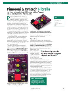


© Copyright 2026