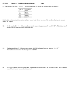
Computers & Industrial Engineering 66 (2013) 889–898
Contents lists available at ScienceDirect
Computers & Industrial Engineering
journal homepage: www.elsevier.com/locate/caie
Solving a reverse supply chain design problem by improved Benders
decomposition schemes q
Ernesto D.R. Santibanez-Gonzalez a,⇑, Ali Diabat b
a
b
Departamento de Computação, Universidade Federal de Ouro Preto, Ouro Preto, MG, Brazil
Department of Engineering Systems & Management, Masdar Institute of Science & Technology, Abu Dhabi, UAE
a r t i c l e
i n f o
Article history:
Received 3 October 2012
Received in revised form 11 May 2013
Accepted 6 September 2013
Available online 18 September 2013
Keywords:
Supply chain management
Reverse logistics
Benders decomposition
Mixed-integer programming
a b s t r a c t
In this paper we propose improved Benders decomposition schemes for solving a remanufacturing supply
chain design problem (RSCP). We introduce a set of valid inequalities in order to improve the quality of
the lower bound and also to accelerate the convergence of the classical Benders algorithm. We also derive
quasi Pareto-optimal cuts for improving convergence and propose a Benders decomposition scheme to
solve our RSCP problem. Computational experiments for randomly generated networks of up to 700
sourcing sites, 100 candidate sites for locating reprocessing facilities, and 50 reclamation facilities are
presented. In general, according to our computational results, the Benders decomposition scheme based
on the quasi Pareto-optimal cuts outperforms the classical algorithm with valid inequalities.
Ó 2013 Elsevier Ltd. All rights reserved.
1. Introduction
Adopting a friendly sustainable management approach implies
a number of changes for companies from the strategic level up to
the operational point of view, affecting their employees and
impacting their business processes and technology. In this regard,
Simchi-Levi, Kaminsky, and Simchi-Levi (2007) point out, ‘‘the
strategic level deals with decisions that have a long-lasting effect
on the ﬁrm. These include decisions regarding the number, location and capacities of warehouses and manufacturing plants, or
the ﬂow of material through the logistics network.’’
The problem of locating facilities and allocating customers is
not new to the operations research community and involves the
key aspects of supply chain design (Daskin, Snyder, & Berger,
2005). This problem is one of ‘‘the most comprehensive strategic
decision problems that need to be optimized for long-term efﬁcient operation of the whole supply chain’’ (Altiparmak, Gen, Lin,
& Paksoy, 2006). As observed by Farahani and Hekmatfar (2009),
some small changes to classical facility location models can make
the problems much harder to solve.
In the last few years, mathematical modeling and solution
methods for the efﬁcient management of return ﬂows (and/or integrated with forward ﬂows) have been studied in the context of reverse logistics, closed-loop supply chains, and sustainable supply
chains.
q
The manuscript was processed by the area editor Qiuhong Zhao.
⇑ Corresponding author. Tel.: +55 31 3559 1692.
E-mail address: [email protected] (E.D.R. Santibanez-Gonzalez).
0360-8352/$ - see front matter Ó 2013 Elsevier Ltd. All rights reserved.
http://dx.doi.org/10.1016/j.cie.2013.09.005
Fleischmann, Krikke, Dekker, and Flapper (2000) discussed new
issues that arise in the context of reverse logistics, and they
reviewed the mathematical models proposed in the literature.
Fleischmann, Beullens, Bloemhof-Ruwaard, and Va (2001) proposed a generic recovery network model based on the elementary
characteristics of return networks identiﬁed in Fleischmann et al.
(2000). Zhou and Wang (2008) proposed a generic mixed integer
model for the design of a reverse distribution network including
repairing and remanufacturing options simultaneously.
Regarding reverse logistics networks in connection with location problems, Bloemhof-Ruwaard, Salomon, and Van Wassenhove
(1996) presented a two-level distribution and waste disposal problem, in which demand for products is met by plants while the
waste generated by production is correctly disposed of at waste
disposal units. Barros, Dekker, and Scholten (1998) described a network for recycling sand from construction waste and proposed a
two-level location model to solve the location problem of two
types of intermediate facilities.
Regarding remanufacturing location models, Krikke, Van
Harten, and Schuur (1999) described a small reverse logistics network for the returns, processing, and recovery of discarded copiers.
They presented a mixed integer linear programming (MILP) model
based on a multi-level uncapacitated warehouse location model.
The model was used to determine the locations and capacities of
the recovery facilities as well as the transportation links connecting various locations. In Jayaraman, Patterson, and Rolland
(2003), a 0–1 MILP model for a product recall distribution problem
is proposed. They analyzed a particular case in which the customer
returns the product to a retail store, and the product is sent to a
890
E.D.R. Santibanez-Gonzalez, A. Diabat / Computers & Industrial Engineering 66 (2013) 889–898
refurbishing site which will rework the product or properly dispose it. The reverse supply chain is composed of origination, collection, and refurbishing sites. With the objective to minimize ﬁxed
and distribution costs, the model has to decide which collection
sites and which refurbishing sites to open, subject to a limit on
the number of collection sites and refurbishing sites that can be
opened.
Several authors have studied different aspects of closed-loop
supply chain problems. See, for example, Jayaraman, Guide, and
Srivastava (1999), Fleischmann (2003), Barbosa-Povoa, Salema,
and Novais (2007), Guide and Van Wassenhove (2009) and Neto,
Walther, Bloemhof-Ruwaard, Van Nunen, and Spengler (2010).
Sahyouni, Savaskan, and Daskin (2007) presented three generic
facility location MIP models for integrated decision making in the
design of forward and reverse logistics networks. The formulations
are based on the well-known uncapacitated ﬁxed-charge location
model, and they include the location of used product collection
centers and the assignment of product return ﬂows to these centers. Lu and Bostel (2007) presented a two-level location problem
with three types of facilities to be located in a reverse logistics system. They proposed a 0–1 MILP model which simultaneously considers ‘‘forward’’ and ‘‘reverse’’ ﬂows and their mutual interactions.
The model has to decide the number and locations of three different types of facilities: producers, remanufacturing centers, and
intermediate centers.
In summary, reverse logistics models are chronologically discussed by Bloemhof-Ruwaard et al. (1996), Barros et al. (1998),
Krikke et al. (1999), Fleischmann et al. (2000, 2001), Shih (2001),
Sodhi and Reimer (2001), Jayaraman et al. (2003), Le Blanc, Fleuren,
and Krikke (2004), Listesß and Dekker (2005), and more recently
Zhou and Wang (2008), Salema, Barbosa-Povoa, and Novais
(2010), Gomes, Barbosa-Povoa, and Novais (2011) and Alumur,
Nickel, Saldanha-da-Gama, and Verter (2012). Almost all of this research proposed MILP models. Listesß and Dekker proposed a stochastic MILP and Alumur et al. studied the dynamic factors that
affect location decisions. The majority of solution methods are
based on standard commercial packages.
In this paper, the problem of designing a reverse supply chain
network is addressed, and a Benders decomposition-based algorithm is proposed for solving it. The problem is a NP-hard combinatorial optimization problem. The MILP model follows some
previously published work by, for example, Jayaraman et al.
(2003), Salema et al. (2010) and Li (2011), but in this paper we develop a more efﬁcient algorithm for solving it. For randomly generated test instances of the problem, we analyze the performance of
the algorithms in term of computational times and quality of the
solution obtained.
This paper makes three primary contributions. First, it proposes
a Benders decomposition algorithm for solving large-scale reverse
network design problems. We test two sets of valid inequalities to
strengthen the Relaxed Master Problem in order to improve the
quality of the lower bound. Second, we derive quasi Pareto-optimal
cuts as another strategy to accelerate convergence, and third, we
propose a primal based Benders decomposition algorithm for solving the problem. Computational results are conducted on largescale networks of up to 700 sourcing facilities, 100 candidate sites
for locating reprocessing facilities, and 50 reclamation facilities
(700 100 50). To the best of our knowledge, for this kind of
problems, these are the largest problems explored and solved so
far.
The remainder of this paper is organized as follows. In the second section, we formulate the mathematical model for the problem. In the third section, the Benders decomposition-based
algorithms for solving the problem are proposed. In the fourth section, we present some strategies for accelerating the convergence
of the Benders algorithms. In the ﬁfth section, the computational
experiments performed with the algorithms are presented. The last
section contains our conclusions.
2. Model for designing a reverse supply chain network
The problem can be categorized as a single product, static,
three-echelon, capacitated location model with known demand.
The reverse supply chain network consists of three types of members: sourcing facilities (origination sites like a retail store), collection sites, and reclamation facilities. At the customer levels, there
are product demands and used products ready to be recovered
(for example, cell phones). We suppose that customers return
products to origination sites like a retail store. At the second layer
of the supply chain network, there are reprocessing centers (collection sites) used only in the reverse channel, and they are responsible for activities such as cleaning, disassembly, checking, and
sorting, before the returned products are sent back to reclamation
facilities. At the third layer, reclamation facilities accept the
checked returns from intermediate facilities and they are responsible for the process of reclamation. In this paper, we address the
backward ﬂow of returns coming from sourcing facilities and going
to reclamation facilities through reprocessing facilities properly located at pre-deﬁned sites. In such a supply chain network, the ‘‘reverse’’ ﬂow moves from customers through collection sites to
reclamation facilities and is formed by used products. On the other
hand, the ‘‘forward’’ ﬂow moves from reclamation facilities directly
to new products at points of sale.
2.1. RSCP model
In this model, it is assumed that new product demands and
available quantities of used products are known and deterministic. All returned (used) products are ﬁrst shipped back to collection facilities where some of them will be discarded for various
reasons, including poor quality. The checked return-products will
then be sent back to reclamation facilities, where some of them
may still be discarded. We introduce the following inputs and
sets:
I
J
the set of sourcing facilities at the ﬁrst layer, indexed by i
the set of reclamation nodes at the third layer indexed by
j
K
the set of candidate reprocessing facility locations at the
mid layer, indexed by k
ai
supply quantity at source location i 2 I
bj
demand quantity at reclamation location j 2 J
fk
ﬁxed cost of locating a mid layer reprocessing facility at
candidate site k 2 K
gk management cost at a mid layer reprocessing facility at
candidate site k 2 K
cik is the unit cost of delivering products at k 2 K from a
source facility located in i 2 I
dkj is the unit cost of supplying demand j 2 J from a mid layer
facility located in k 2 K
mk capacity at reprocessing facility location k 2 K
We consider the following decision variables:
wk 1 if we locate a reprocessing facility at candidate site
k 2 K, 0 otherwise
xik ﬂow from source facility i 2 I to reprocessing facility
located at k 2 K
ykj ﬂow from reprocessing facility located at k 2 K to facility
j2J
Following the model proposed by Li (2011), the reverse supply
chain design problem (RSCP) is deﬁned by:
E.D.R. Santibanez-Gonzalez, A. Diabat / Computers & Industrial Engineering 66 (2013) 889–898
891
Fig. 1. Reverse supply chain network.
X
XX
XX
Minimize
fk wk þ
ðcik þ g k Þxik þ
dkj ykj
i2I k2K
k2K
X
xik 6 mk wk
ð1Þ
k2K j2J
8k 2 K
ð2Þ
i2I
X
xik 6 ai
8i 2 I
ð3Þ
8j 2 J
ð4Þ
k2K
X
ykj P bj
k2K
X
X
xik ¼
ykj
i2I
8k 2 K
ð5Þ
jJ
xik ; ykj P 0;
8i 2 I; 8j 2 J; 8k 2 K
wk 2 f0; 1g 8k 2 K
ð6Þ
ð7Þ
The objective function (1) minimizes the sum of the installation
reprocessing facility costs plus management costs at the reprocessing facilities plus delivery costs from sourcing facilities to reprocessing facilities and from these to reclamation facilities.
Constraints (2) ensure that all of the products that arrive at reprocessing site k 2 K must be less than its capacity and that this facility
must be opened. Constraints (3) guarantee that up to a volume of ai
return products available at i are going backward to facility k 2 K.
Constraints (4) warrant that the demand at facility j 2 J must be satisﬁed by reprocessing facilities. Constraints (5) ensure that all the
return products arriving to facility k are also delivered to reclamation facilities. Constraints (6) are the standard nonnegative constraints. Constraints (7) are the standard binary constraints. This
model has O(n2) continuous variables where n = max{|I|, |J|, |K|}
and |K| are binary variables. The number of constraints is O(n).
Fig. 1 shows a reverse supply chain network consisting of 6
groups of customers, 8 candidate sites for locating reprocessing
facilities (with three facilities opened), and two reclamation
facilities.
3. Benders decomposition
Benders decomposition is a classical decomposition technique
(Benders, 1962) which is advisable for solving hard mixed integer
programming problems with integer variables and coupling constraints. Benders decomposition technique involves decomposing
the overall formulation into a Master problem and a (Benders) subproblem, and then solving them iteratively by utilizing the solution
of one in the other. The Benders Master problem with only integer
variables and an auxiliary variable is a relaxation of the primary
problem. The auxiliary variable is introduced to facilitate the interaction between the Master problem and the subproblem. In a minimization problem, an optimal solution of the Benders Master
problem provides a lower bound on the original problem and the
values of the integer variables are passed through the subproblem
for solving a new subproblem. By ﬁxing the integer variables, the
primary problem with only continuous variables becomes a Benders subproblem that can be solved easily. By solving the subproblem, the values of its dual variables and a valid upper bound for the
primary problem (in the case of minimization) are obtained, and, in
this case, by utilizing its objective value along with the cost components implied by the Master problem solution. The bounds are
updated, and if the stopping criterion is not met, a Benders cut
using the dual subproblem solution is generated. This new cut is
appended to the Master problem, and the Benders decomposition
algorithm is iterated continuously until a stopping criterion is
met. To establish a stopping criteria, we employ a small percentage
gap between the best upper and lower bounds and a maximum
number of Benders cycles reached; whatever is achieved ﬁrst ends
the algorithm.
There are a number of publications to support the fact that the
Benders algorithm has not been uniformly successful in all applications; it has some deﬁciencies. Geoffrion and Graves (1974), among
others, have noted that reformulating a mixed integer program can
have a profound effect upon the efﬁciency of the algorithm. For the
particular case of a network design problem (Magnanti & Wong,
1981), it has been observed that a straightforward implementation
of the Benders algorithm often converged very slowly, requiring
the solution of a large number of Relaxed Master Problems. The
main issues associated with slow convergence of Benders algorithms are (a) the solution of Relaxed Master Problems and Benders subproblems, and (b) the quality of the cuts produced in each
iteration. To overcome these issues, accelerating techniques have
been studied by a number of authors, among them: McDaniel
and Devine (1977), Magnanti and Wong (1981), Côté and Laughton
(1984), Papadakos (2008), Rei, Cordeau, Gendreau, and Soriano
(2008), Saharidis, Minoux, and Ierapetritou (2010), Sherali and
Lunday (2011) and Tang, Jiang, and Saharidis (2012). In a seminal
paper, Magnanti and Wong (1981) proposed generating more than
one cut in each iteration to accelerate the Benders algorithm, using
what they refer to as Pareto-optimal cuts. A cut is deﬁned as Pareto-optimal if no other cut dominates it. The authors propose to
add, in each iteration of the algorithm, two types of cuts: the optimality or feasibility cut produced by the classical Benders procedure, and also the Pareto-optimal cuts. The results obtained by
their approach showed a signiﬁcant improvement in the algorithm
convergence.
In the context of facility location problems, the Benders decomposition algorithm has been successfully applied by many
researchers. Among them, Geoffrion and Graves (1974) employed
the Benders decomposition algorithm to solve the two-stage distribution system design problem. Dogan and Goetschalckx (1999)
studied the integrated design problem of a multi-period production–distribution system. Cordeau, Pasin, and Solomon (2006)
solved an integrated model for a logistics network design problem,
and Wentges (1996) used Pareto-optimal cuts and a procedure to
892
E.D.R. Santibanez-Gonzalez, A. Diabat / Computers & Industrial Engineering 66 (2013) 889–898
strengthen Benders cuts to speed up the Benders decomposition
algorithm for a discrete capacitated facility location problem.
In this paper, we will use Benders decomposition algorithms to
solve a reverse supply chain design problem. We derive a series of
valid inequalities (VI) to add to the Benders Master problem to restrict its solution space. We enter these VIs into a classical Benders
decomposition algorithm to solve the problem. We also propose a
Pareto-optimal cut strategy to generate cuts and we test it in order
to accelerate the convergence and to evaluate the impact on the
quality of the bounds obtained. Regarding the Pareto-optimal
strategy, we propose to use a primal–dual Benders decomposition
algorithm to generate quasi Pareto-optimal cuts and to solve the
problem. The algorithms are compared in terms of speed of convergence and quality of the bounds generated.
3.1. Decomposition scheme
Minimize
þ
cT2 y
Subject to Ax þ By 6 b
ð8Þ
ð9Þ
xP0
ð10Þ
y 2 f0; 1g
ð11Þ
Applying Benders decomposition to this problem, the decision
variables are partitioned into two sets: x and y, and the principal
problem is decomposed into the Relaxed Master Problem (RMP)
and a series of Benders subproblems (BSP).
€ in PP, the general form of the
Fixing integer variables y ¼ y
Benders subproblem is as follows:
(BSP)
Minimize cT1 x
ð12Þ
€
Subject to Ax 6 b By
ð13Þ
xP0
ð14Þ
The dual problem of BSP (D-BSP) can be written as
(D-BSP)
T
ð15Þ
cT1
ð16Þ
€Þ u
Maximize ðb By
T
Subject to A u 6
u60
3.2. Subproblem
€ k , the primal
By ﬁxing binary (facility location) variables wk ¼ w
Benders subproblem (PBS) in our RSCP problem is as follows:
(PBS)
i2I k2K
And the general form of the Master Problem (MP) is as follows:
(MP)
ð18Þ
T
ð19Þ
€Þ ðuq Þ 6 0
ðb By
T
ð20Þ
y 2 f0; 1g
ð21Þ
€Þ ðup Þ 6 z
Subject to ðb By
ð22Þ
k2K j2J
X
€k
xik 6 mk w
Subject to
8k 2 K
ð23Þ
i2I
X
xik 6 ai
8i 2 I
ð24Þ
8j 2 J
ð25Þ
k2K
X
ykj P bj
k2K
X
X
xik P
ykj
i2I
8k 2 K
ð26Þ
j2J
xik ; ykj P 0;
8i 2 I; 8j 2 J; 8k 2 K
ð27Þ
Notice that, without loss of generality, constraint (26) replaces
constraint (5), considering that,
X
X
ai P
bj
i2I
ð28Þ
j2J
Deﬁning dual variables uk associated with constraint (23), si associated with constraint (24), associated with constraint (25), and qk
associated with constraint (26), we can write the dual of the PBS
problem (DBS) as follows:
(DBS)
Maximize
X
X
X
€ k uk þ
bj r j mk w
ai si
j2J
!
ð29Þ
i2I
k2K
8i 2 I; 8k 2 K
8j 2 J; 8k 2 K
qk ; r j ; si ; uk P 0; 8i 2 I; 8j 2 J; 8k 2 K
Subject to qk si uk P 0;
qk r j P 0;
ð30Þ
ð31Þ
ð32Þ
By duality theory, if the PBS problem is infeasible for the ﬁxed val€ k , then the DBS problem has a bounded solution which is an
ues w
extreme point of the polyhedron X constituted by (30)–(32), and
thus an optimality Benders cut is deduced, taking the form in
(33). If the PBS problem is infeasible, the DBS problem has an unbounded solution, an extreme ray of the polyhedron can be identiﬁed, and a feasibility Benders cut will be generated taking the form
in (34).
Let PX and QX be the sets of all the extreme points and extreme
rays of polyhedron X, respectively; z an auxiliary variable, then the
optimality and feasibility Benders cuts are as follows:
ð17Þ
Minimize cT1 x þ z
XX
XX
ðcik þ g k Þxik þ
dkj ykj
Minimize
Consider the special structure of our formulation that facilitates
a decomposition approach. Notice that the integer variables, w, and
the ﬂows variables, x and y, are related decisions and that constraint (2) is a coupling constraint. We observe that by ﬁxing the
number and location of facilities, i.e., for ﬁxed w values, we get a
linear program that can be solved efﬁciently. Utilizing this structure, in our Benders decomposition based solution algorithm, the
Master problem includes the binary integer location decisions
and the subproblem determines the ﬂows of return products from
the sourcing sites to reclamation facilities throughout reprocessing
facilities already opened.
To simplify, consider the following mixed integer linear programming Principal Problem (PP), where the vector y contains a
number of facility location variables which are considered complicated variables, while vector x contains a number of return ﬂows
positive variables.
(PP)
cT1 x
where up and uq are vectors of extreme points and extreme rays,
respectively, of the polyhedron formed by constraints (16) and
(17), and z is an auxiliary continuous variable. The main drawback
of MP is that the dimension of vectors up and uq is usually extremely
large. To overcome this limitation, the Benders algorithm proposes
to generate constraints (19) and (20) iteratively, as we will explain
later in this paper.
Following the Benders decomposition scheme described above,
for our RSCP problem, we obtain the following problems:
zP
X p
X
X p
€ k upk þ
bj r j mk w
ai si
j2J
k2K
!
ð33Þ
i2I
and
X Q
X
X Q
€ k uQk þ
0P
bj r j mk w
ai si
j2J
k2K
p
!
i2I
where r pj ; spi anduk PX and r Qj ; sQi and uQk Q X .
ð34Þ
E.D.R. Santibanez-Gonzalez, A. Diabat / Computers & Industrial Engineering 66 (2013) 889–898
893
Tragantalerngsak, Holt, and Rönnqvist (2000) proposed to improve the relaxation of a related capacitated location problem by
introducing a constraint of the following type:
X
wk P 1
ð39Þ
k2K
Constraint (39) forces the selection of at least one facility to be open.
(2) Feasibility – facilities servicing the demand – wcon1
X
X
€k P
mk w
bj
k2K
ð40Þ
j2J
Constraint (40) ensures that opened reprocessing facilities have enough capacity to service all the demand for returned products at
reclamation facilities.
4.2. Generation of Pareto-optimal cuts
Fig. 2. Pseudo-code for a classical Benders decomposition algorithm.
3.3. Relaxed Master Problem
Based on the cuts of type (33) and (34) described above, the Relaxed Master Problem (RMP) in our RSCP can be written as follows:
(RMP)
Minimize
X
fk wk þ z
ð35Þ
k2K
Subject to
X p
X
X p
€ k upk þ
zP
bj r j mk w
a i si
j2J
k2K
j2J
k2K
ð36Þ
i2I
!
ð37Þ
i2I
wk 2 f0; 1g 8k 2 K
T
Maximize ðb Byþ Þ u
T
Subject to A u 6
ð41Þ
cT1
T
ð42Þ
€Þ u 6 ðb By
€ÞT u
ðb By
u60
ð38Þ
The optimality Benders cuts (36) can strengthen the lower
bound obtained from the RMP problem while the feasibility Benders cuts (37) make the lower bound valid for the RSCP primary
problem.
€Þ u is the optimal objective value of the dual subwhere ðb By
problem (D-BSP) and y+ is a core point of the solution space of the
Relaxed Master problem (RMP).
For our problem, we use the following two facts for deriving
Pareto-optimal cuts:
any extreme point or any extreme ray of the dual subproblem
gives a valid Benders cut (Benders, 1962);
it is not necessary to use a core point of the solution space of the
Master problem to produce a Pareto cut (Papadakos, 2008).
Then, the following auxiliary problem can produce Pareto-optimal cuts:
(APO)
T
3.4. Benders decomposition algorithm
In Fig. 2 we show the pseudo-code of a classical Benders decomposition algorithm. We use this scheme jointly with the valid
inequalities described in the next section.
4. Strategies for accelerating Benders decomposition algorithm
4.1. Valid inequalities
We derive a series of valid inequalities to strengthen the Master
problem and to improve the lower bound provided by the Benders
decomposition algorithm. As described earlier in this paper, one of
the reasons for slow convergence of the Benders decomposition
algorithm is that the lower bound provided by the RMP problem
could be relatively weak.
According to the structure of our problem, we developed the
following valid inequality (VI) to narrow the solution space of
the RMP:
(1) Forcing to open at less than one facility – wcon
ð43Þ
ð44Þ
T
!
X Q
X
X Q
€ k uQk þ
0P
bj r j mk w
ai si
The BSP problem has a network structure; hence, it typically has
multiple dual solutions as an alternative for the optimality cut
computed by (36). We would like to generate a cut that dominates
others’ cuts in the vicinity of the optimal solution. According to
Magnanti and Wong (1981), a Pareto-optimal cut can be obtained
by solving the following problem:
(PO-BSP)
Maximize ðb By Þ u
ð45Þ
Subject to AT u 6 cT1
T
€Þ 6
ðb By
ð46Þ
cT1 x
u60
ð47Þ
ð48Þ
where cT1 x is the optimal objective value of the primal subproblem
(BSP) and y- is the linear relaxation solution of the Master problem.
Fig. 3 depicts the pseudo-code of a classical Benders decomposition algorithm considering the procedure for generating
Pareto-optimal cuts (Cordeau et al., 2006; Magnanti & Wong,
1981; Papadakos, 2008). Observe that it includes the auxiliary
problem solution for obtaining the Pareto-optimal cuts, after
solving the DSP problem. That is because it used the optimal solution of the DSP for generating the optimality cut to be included in
the Master problem. As explained before, the core point is obtained
by getting the LP solution of the Master problem.
5. Computational experiments
In this section we describe computational experiments using
the proposed Benders decomposition methods for solving
894
E.D.R. Santibanez-Gonzalez, A. Diabat / Computers & Industrial Engineering 66 (2013) 889–898
Fig. 3. Pseudo-code for a classical Benders decomposition algorithm with Pareto-optimal cuts.
large-scale reverse supply chain design problems. We ﬁrst describe
the characteristics of the test problems and some implementation
details, and then we demonstrate the computational efﬁciencies
achieved by each of the Benders decomposition methods in terms
of computing times, quality of the lower and upper bounds, and
the number of Benders cycles.
To evaluate the impact of employing the different proposed valid inequalities (VI), we solve each instance with our Benders algorithm, given in Fig. 1, both with and without the proposed VI. The
effects of the different types of cuts on the performance of the
Benders decomposition algorithm are compared and the computational results are reported. The Benders decomposition algorithms
are coded in GAMS and tested on the computer with CPU of
2.3 GHz and 4.0 GB RAM. Whenever Benders decomposition algorithms are needed to solve the Master problem and Benders subproblems, CPLEX (version 12.3) with default settings is used as
an optimization solver.
The Benders decomposition algorithms stopped when one of
the following criteria was reached:
(i) the optimality gap (100 (zub–zlb)/zlb) was below a threshold
value e = 0.009;
(ii) the maximum number of iterations (Benders cycles) was hit:
we set it to 50.
For the alternative types of VI and Pareto-optimal cuts, the progression of zub and zlb values over the iterations is depicted in Fig. 4.
For space limitation, we plot the results for a problem instance of
600 100 40. We can observe that the use of proposed VI of type
wcon1 is effective in speeding up convergence and that the quality
of both the upper and lower bounds is affected. We also observe
the same effects when using the Pareto optimal cuts. Note that,
in the case of the Pareto-optimal cuts, we developed an alternative
Benders decomposition algorithm based on the solution of a primal
subproblem. Fig. 4 represents what we observe in our numerical
studies with other instances: a similar high performance in convergence with cuts and, in particular, with a VI of type wcon1. We observe that alternative Benders decomposition algorithms with
Pareto optimal cuts converge very quickly to the best lower bound.
Fig. 4. Upper and lower bounds provided by the different Benders algorithms for
problem instance 9.
ies according to the number of sourcing facilities (|I|), the number
of candidate sites for locating reprocessing facilities (|K|), and the
number of reclamation facilities (|J|). The data set for the test problems is given in Table 1. All the transportation costs were generated randomly using a uniform distribution with parameters
[1, 40]. Management costs (gk) were set to 30 for all problem instances. Fixed costs (fk) for problem instances 6–10 were obtained,
multiplying by 10 the ﬁxed costs of the corresponding reprocessing
facilities of problem instances 1–5. Sourcing units (ai), the capacity
of reprocessing facilities (mk), and the capacity of reclamation facilities (bj) are shown in Table 1.
To illustrate the size differences between the problem instances
of the RSCP model, for problem instances 1–5, Table 2 shows the
number of continuous and binary variables as well as the number
of constraints.
5.2. Results analysis
5.1. Data generation
We randomly generated a set of 10 instances ranging from networks of 350 sourcing facilities, 100 candidate sites for locating
reprocessing
facilities,
and
40
reclamation
facilities
(350 100 40) up to 700 100 40. The size of an instance var-
In Table 3, the lower and upper bounds, gap (%), and number of
Benders cycles are presented for Benders algorithms without any
additional VI and with VI of type wcon. These VI do not produce
any signiﬁcant impact, neither on the gap nor in the number of
Benders cycles. To illustrate, for problem instance 3, gaps and
895
E.D.R. Santibanez-Gonzalez, A. Diabat / Computers & Industrial Engineering 66 (2013) 889–898
Table 1
Data set.
#
Instance problems
|I|
|K|
|J|
fk
ai
mk
bj
1
2
3
4
5
6
7
8
9
10
350 100 40
400 100 40
500 100 40
600 100 40
700 100 40
350 100 40
400 100 40
500 100 40
600 100 40
700 100 40
350
400
500
600
700
350
400
500
600
700
100
100
100
100
100
100
100
100
100
100
40
40
40
40
40
40
40
40
40
40
2000
2000
2000
2500
3000
20,000
20,000
20,000
25,000
30,000
200
200
200
300
300
200
200
200
300
300
800
1500
1500
3000
3000
800
1500
1500
3000
3000
1750
2000
2500
2500
2500
1750
2000
2500
2500
2500
Table 2
Size formulation for problem instances 1–5.
Instance
Continuous variables
Binary variables
Number of constraints
1
2
3
4
5
39,000
44,000
54,000
64,000
74,000
100
100
100
100
100
590
640
740
840
940
Benders cycles are 0.869% and 9 respectively for both algorithms.
When the algorithm hits the maximum number of Benders cycles
(50), gaps provided by the Benders algorithms with cuts wcon is
slightly lesser than those provided without any VI, except for problem instance 9. This is a consequence of an upper bound slightly
worse than that achieved by the Benders decomposition algorithm
with VI of type wcon. To illustrate, for problem instance 4, the
upper bounds are 3,357,200 and 3,354,300 for the Benders algorithm without any VI and with VI of type wcon, respectively. For
problem instance 5, gaps provided by both algorithms are the
same. Regarding lower bounds, both algorithms present the same
values.
In Table 4, the lower and upper bounds, gap (%) and number of
Benders cycles are presented for Benders algorithm with VI of type
wcon1 and for the alternative Benders algorithm with Pareto optimal cuts. The Benders algorithm with VI of type wcon1 presents
good results compared with the alternative Bender algorithm with
Pareto optimal cuts. In some problem instances – for example, 2, 4,
and 8 – gaps achieved by Benders algorithm with VI of type wcon1
are better than those provided by the alternative Benders algorithm. However, gaps are very similar between the two algorithms.
Notice that for those instances, the alternative Benders algorithm
has a smaller number of Benders cycles except for problem instance 4, where both algorithms have the same number. For problem instances 1, 3, 5, 7, and 9–10, gaps provided by the alternative
Benders algorithm are the best. In particular for problem instance
9, a network of 600 100 40, the alternative Benders algorithm
required 13 Benders cycles to achieve a gap of 0.866%, while the
Benders algorithm with VI of type wcon1 required 50 Benders cycles – and hit the limit – to get a gap of 0.922%. However, in Table 8,
we can observe that the smaller number of Benders cycles of the
alternative Benders algorithm did not mean smaller computing
times. On the contrary, the alternative Benders algorithm has the
biggest computing times as a consequence of the time spending
in solving the auxiliary problem to generate the Pareto optimal
cuts. As observed by other authors, in our problem, the time spent
to generate the optimal cuts at each iteration does not necessarily
compensate with a reduction in the number of iterations and the
total resolution time of the problem (Mercier & Soumis, 2007).
Table 5 presents a summary of gaps and Benders cycles for the
different Benders algorithms. To illustrate, for problem instance 9,
gaps are 1.042%, 0.922%, 1.084% and 0.866% for the Benders
algorithm without any VI, with VI of type wcon1, wcon and the
Table 3
Lower bound (zlb), upper bound (zub), gap and number of Benders cycles.
Instances
1
2
3
4
5
6
7
8
9
10
Benders algorithm without any VI
Benders algorithm with VI wcon
zlb
zub
Gap (%)
Benders cycles
zlb
zub
Gap (%)
Benders cycles
2457900
2715200
3371300
3312700
3314000
4041900
3687200
4577300
4077700
4232000
2466000
2737200
3400600
3357200
3344500
4048550
3720100
4609900
4120200
4269000
0.330
0.810
0.869
1.343
0.920
0.165
0.892
0.712
1.042
0.874
5
22
9
50
50
6
9
7
50
9
2457900
2715200
3371300
3312700
3314000
4041900
3687200
4577300
4077600
4232000
2466000
2737200
3400600
3354300
3344500
4048550
3720100
4609900
4121800
4269000
0.330
0.810
0.869
1.256
0.920
0.165
0.892
0.712
1.084
0.874
5
22
9
50
50
4
7
5
50
8
Table 4
Lower bound (zlb), upper bound (zub), gap and number of Benders cycles.
Instances
1
2
3
4
5
6
7
8
9
10
Benders algorithm – VI wcon1
Benders algorithm with Pareto optimal cuts
zlb
zub
Gap (%)
Benders cycles
zlb
zub
Gap (%)
Benders cycles
2457900
2715200
3371300
3312700
3314000
4041900
3687200
4577300
4077700
4232000
2465050
2738000
3397800
3355400
3346500
4048500
3716600
4598700
4115300
4267000
0.291
0.840
0.786
1.289
0.981
0.163
0.797
0.468
0.922
0.827
2
24
10
50
21
2
4
5
50
7
2457900
2715200
3371300
3312700
3314000
4041900
3687200
4577300
4077700
4232000
2464300
2738600
3395700
3369000
3342000
4048500
3715400
4618300
4113000
4258500
0.260
0.862
0.724
1.700
0.845
0.163
0.765
0.896
0.866
0.626
2
22
12
50
22
2
4
4
13
5
896
E.D.R. Santibanez-Gonzalez, A. Diabat / Computers & Industrial Engineering 66 (2013) 889–898
Table 5
Summary gap and number of Benders cycles – different Benders decomposition algorithms.
Instances
Without any VI
VI wcon1
VI wcon
Pareto-optimal cuts
Gap (%)
Benders cycles
Gap (%)
Benders cycles
Gap (%)
Benders cycles
Gap (%)
Benders cycles
1
2
3
4
5
6
7
8
9
10
0.330
0.810
0.869
1.343
0.920
0.165
0.892
0.712
1.042
0.874
5
22
9
50
50
6
9
7
50
9
0.291
0.840
0.786
1.289
0.981
0.163
0.797
0.468
0.922
0.827
2
24
10
50
21
2
4
5
50
7
0.330
0.810
0.869
1.256
0.920
0.165
0.892
0.712
1.084
0.874
5
22
9
50
50
4
7
5
50
8
0.260
0.862
0.724
1.700
0.845
0.163
0.765
0.896
0.866
0.626
2
22
12
50
22
2
4
4
13
5
Ave
Max
Min
0.796
1.343
0.165
21.7
50
5
0.736
1.289
0.163
17.5
50
2
0.791
1.256
0.165
21
50
4
0.771
1.700
0.163
14.9
50
2
Table 6
Summary of initial and last lower bound – different Benders decomposition algorithms.
#
1
2
3
4
5
6
7
8
9
10
Without any VI
VI wcon1
VI wcon
Pareto-optimal cuts
Initial
Last
Initial
Last
Initial
Last
Initial
Last
2355500
2630200
3269800
3227000
3215000
2356300
2631200
3271800
3227700
3215000
2457900
2715200
3371300
3312700
3314000
4041900
3687200
4577300
4077700
4232000
2457900
2715200
3371300
3312700
3314000
4041900
3687200
4577300
4077700
4232000
2457900
2715200
3371300
3312700
3314000
4041900
3687200
4577300
4077700
4232000
2355500
2630200
3269800
3230200
3215000
2373900
2648200
3288800
3252600
3242000
2457900
2715200
3371300
3312700
3314000
4041900
3687200
4577300
4077600
4232000
2457900
2715200
3371300
3312700
3314000
4041900
3687200
4577300
4077700
4232000
2457900
2715200
3371300
3312700
3314000
4041900
3687200
4577300
4077700
4232000
alternative Benders algorithm with Pareto optimal cuts, respectively. For the same instance, the number of Benders cycles is 13
for the alternative Benders algorithm and 50 for all other algorithms. For problem instances 2, 4 and 8, the alternative Benders
algorithm gap is worse than that obtained for the others’ algorithms. In all other cases, alternative Benders algorithms perform
better in term of gaps and Benders cycles, except for the problem
instances mentioned above. The minimum average number of
Benders cycles is obtained by the alternative Benders decomposition algorithm with Pareto optimal cuts, while the minimum average gap is obtained by the Benders algorithm with VI of type
wcon1.
Table 6 presents the initial (iLB) and the last lower bounds (zlb)
obtained by each Benders algorithm. Notice that the Benders algorithm with VI of type wcon1 and the alternative Benders algorithm
obtain the best lower bound in the ﬁrst iteration (Benders cycle) of
the algorithm. Comparing the other two Benders algorithms, we
observe that there is not a signiﬁcant difference between the lower
bounds provided by them. Table 7 shows the relative difference in
percentage between the initial lower bound (iLB) and the last lower bound (100 [iLB zlb]/iLB) provided by the Benders algorithm
(without any VI) and the Benders algorithm with VI of type wcon.
This percentage represents an improvement percentage of the lower bound over the initial lower bound. Note that the maximum relative difference is 71.5% and 70.3% for the Benders algorithm and
the Benders algorithm with VI of type wcon, respectively.
Table 8 reports the computational times (in seconds) required
for the different Benders algorithms to obtain an integer solution
within 0.9% of optimality. We observe that, in general, computational times are mostly well below 91 s. The Benders decomposition algorithm based on Pareto-optimal cuts presents the highest
computational time. This is true for problem instances 2, 3, 4, 5,
Table 7
Relative difference between the initial and the last lower bound provided by Benders
algorithms.
Instances
Without any VI
relative difference (%)
VI wcon relative
difference (%)
1
2
3
4
5
6
7
8
9
10
4.35
3.23
3.10
2.63
3.08
71.54
40.13
39.90
26.33
31.63
4.35
3.23
3.10
2.55
3.08
70.26
39.23
39.18
25.36
30.54
Table 8
Computational times (s) for the Benders algorithms.
Instances
Without any VI
time (s)
VI wcon1
time (s)
VI wcon
time (s)
Pareto-optimal
cuts time (s)
1
2
3
4
5
6
7
8
9
10
4.219
13.853
7.715
35.480
34.643
4.797
6.739
6.901
34.345
8.354
1.708
14.543
8.580
30.628
34.361
1.896
3.144
4.390
30.869
5.706
4.156
14.096
7.739
31.646
34.552
3.244
5.110
4.851
32.033
7.276
3.056
30.458
21.422
91.731
44.324
3.167
5.802
7.462
31.070
10.433
8 and 10. We note that the Benders decomposition algorithm using
wcon1 cuts in general performs well in terms of computational
E.D.R. Santibanez-Gonzalez, A. Diabat / Computers & Industrial Engineering 66 (2013) 889–898
times. This algorithm presents the smallest computational time for
problem instances 1, 4, 5, 6, 7, 8, 9 and 10. For problem instances 2
and 3, the Benders decomposition algorithm using wcon1 cuts presents the worst computational time. For our problem, considering
the quality of the lower and upper bounds obtained by the Benders
decomposition algorithm using wcon1 cuts and the computational
time it spent in obtaining these bounds, the relative performance
of this algorithm is good. Furthermore, as it was observed for other
problems (Saharidis, Boile, & Theofanis, 2011; Tang et al., 2012), a
strong valid inequality, like the wcon1, can help to accelerate the
convergence of the Benders algorithm by providing an improved
lower bound (the best lower bound in seven out of ten, excluding
Benders algorithm with Pareto-optimal cuts) and that can also
eventually compensate the increase in the total resolution time
produced by the poor quality of the optimality cuts generated by
the Benders subproblem (without using Pareto-optimal cuts).
6. Conclusions
In this paper, we analyzed a reverse and sustainable supply
chain network design problem. This is a NP-hard combinatorial
problem and it addresses the design of a supply network that consists of three types of members: sourcing facilities (sources), reprocessing facilities, and reclamation facilities. We need to locate
reprocessing facilities in order to minimize the ﬂow cost from
the origination sites to the reclamation facilities through reprocessing facilities. We proposed Benders decomposition algorithms
for solving the problem. In order to accelerate the convergence of
the algorithm and to improve the quality of the lower bounds,
we proposed two sets of valid inequalities. One of them proved
to have a signiﬁcant impact on the quality of the lower bound.
As a second strategy to accelerate convergence of the algorithm,
we derived quasi Pareto-optimal cuts and proposed a primal based
Benders decomposition algorithm for solving the problem. Both
algorithms were compared and, in some problem instances, in
terms of the quality of lower and upper bounds, computational results provided better performance for the primal based Benders
decomposition algorithm with Pareto-optimal cuts. But in terms
of total resolution time, this algorithm presents the highest values.
As observed by other authors (for example, Mercier and Soumis,
2007; Sherali and Lunday, 2011), the time required to generate
Pareto-optimal cuts does not necessarily offset the total resolution
time. On the other hand, introducing a wcon1 valid inequality into
the Master problem from the ﬁrst iteration proved to be an effective way to accelerate convergence; in addition, the ﬁrst lower
bound obtained by solving the Relaxed Master Problem was significantly improved. This algorithm presents the smallest computational time in eight out of ten problem instances. The ﬁnal gap
provided by this algorithm does not present a signiﬁcance difference (less than 0.2%) when compared with the best gap provided
by the Benders algorithm with Pareto-optimal cuts. We can conclude that, for this problem, a Benders algorithm with a strong valid inequality presents a good performance in terms of gap and
total resolution time.
References
Altiparmak, F., Gen, M., Lin, L., & Paksoy, T. (2006). A genetic algorithm approach for
multi-objective optimization of supply chain networks. Computers & Industrial
Engineering, 51(1), 196–215. http://dx.doi.org/10.1016/j.cie.2006.07.011.
Alumur, S. A., Nickel, S., Saldanha-da-Gama, F., & Verter, V. (2012). Multi-period
reverse logistics network design. European Journal of Operational Research,
220(1), 67–78. http://dx.doi.org/10.1016/j.ejor.2011.12.045.
Barbosa-Povoa, A. P., Salema, M. I. G., & Novais, A. Q. (2007). Design and planning of
closed loop supply chains. In L. G. Papageorgiou & M. C. Georgiadis (Eds.), Supply
chain optimization (pp. 187–218). Wiley.
897
Barros, A. I., Dekker, R., & Scholten, V. (1998). A two-level network for recycling
sand: A case study. European Journal of Operational Research, 110(2), 199–214.
http://dx.doi.org/10.1016/S0377-2217(98)00093-9.
Benders, J. F. (1962). Partitioning procedures for solving mixed-variables
programming problems. Numerische Mathematik, 4(1), 238–252.
Bloemhof-Ruwaard, J., Salomon, M., & Van Wassenhove, L. N. (1996). The
capacitated distribution and waste disposal problem. European Journal of
Operational Research, 88, 490–503. <http://www.sciencedirect.com/science/
article/pii/0377221794002118>.
Cordeau, J.-F., Pasin, F., & Solomon, M. M. (2006). An integrated model for logistics
network design. Annals of Operations Research, 144(1), 59–82. http://dx.doi.org/
10.1007/s10479-006-0001-3.
Côté, G., & Laughton, M. A. (1984). Large-scale mixed integer programming:
Benders-type heuristics. European Journal of Operational Research, 16(3),
327–333. http://dx.doi.org/10.1016/0377-2217(84)90287-X.
Daskin, M. S., Snyder, L. V., & Berger, R. T. (2005). Facility location in supply chain
design. In A. Langevin & D. Riopel (Eds.), Logistics systems: Design and
optimization (pp. 39–65). Kluwer.
Dogan, K., & Goetschalckx, M. (1999). A primal decomposition method for the
integrated design of multi-period production–distribution systems. IIE
Transactions, 31(11), 1027–1036. http://dx.doi.org/10.1080/07408179908969904.
Farahani, R. Z., & Hekmatfar, M. (2009). Facility location: Concepts, models, algorithms
and case studies. In R. Zanjirani Farahani & M. Hekmatfar (Eds.), Media (pp. 549).
Springer-Verlag. <http://www.dx.doi.org/10.1007/978-3-7908-2151-2>.
Fleischmann, Moritz, Beullens, P., Bloemhof-Ruwaard, J. M., & Va, L. N. (2001). The
impact of product recovery on logistics network design. Production and
Operations Management, 10(2), 156–173.
Fleischmann, Moritz (2003). Reverse logistics network structures and design. In V.
D. R. Guide & L. N. Van Wassenhove (Eds.), Business aspects of closed-loop supply
chains (pp. 117–135). New York: Carnegie Mellon University Press.
Fleischmann, Mortiz, Krikke, H. R., Dekker, R., & Flapper, S. D. P. (2000). A
characterisation of logistics networks for product recovery. Omega, 28(6),
653–666. http://dx.doi.org/10.1016/S0305-0483(00)00022-0.
Geoffrion, A., & Graves, G. (1974). Multicommodity distribution system design by
Benders decomposition. Management science, 20(5), 822–844.
Gomes, M. I., Barbosa-Povoa, A. P., & Novais, A. Q. (2011). Modelling a recovery
network for WEEE: A case study in Portugal. Waste Management (New York, NY),
31(7), 1645–1660. http://dx.doi.org/10.1016/j.wasman.2011.02.023.
Guide, V. D. R., & Van Wassenhove, L. N. (2009). OR FORUM – The evolution of
closed-loop supply chain research. Operations Research, 57(1), 10–18. http://
dx.doi.org/10.1287/opre.1080.0628.
Jayaraman, V., Guide, V. D. R., & Srivastava, R. (1999). A closed-loop logistics model
for remanufacturing. Journal of the Operational Research Society, 50(5), 497–508.
http://dx.doi.org/10.1057/palgrave.jors.2600716.
Jayaraman, Vaidyanathan, Patterson, R. A., & Rolland, E. (2003). The design of
reverse distribution networks: Models and solution procedures. European
Journal of Operational Research, 150(1), 128–149. http://dx.doi.org/10.1016/
S0377-2217(02)00497-6.
Krikke, H. R., Van Harten, A., & Schuur, P. C. (1999). Business case Océ: Reverse
logistic network re-design for copiers. OR Spectrum, 21(3), 381–409. http://
dx.doi.org/10.1007/s002910050095.
Le Blanc, H. M., Fleuren, H. A., & Krikke, H. R. (2004). Redesign of a recycling system
for LPG-tanks. OR Spectrum, 26(2), 283–304. http://dx.doi.org/10.1007/s00291003-0145-3.
Li, N. (2011). Research on location of remanufacturing factory based on particle
swarm optimization. MSIE 2011 (pp. 1016–1019). IEEE. doi: http://dx.doi.org/
10.1109/MSIE.2011.5707588.
Listesß, O., & Dekker, R. (2005). A stochastic approach to a case study for product
recovery network design. European Journal of Operational Research, 160(1),
268–287. http://dx.doi.org/10.1016/j.ejor.2001.12.001.
Lu, Z., & Bostel, N. (2007). A facility location model for logistics systems including
reverse ﬂows: The case of remanufacturing activities. Computers & Operations
Research, 34(2), 299–323. http://dx.doi.org/10.1016/j.cor.2005.03.002.
Magnanti, T., & Wong, R. (1981). Accelerating Benders decomposition: Algorithmic
enhancement and model selection criteria. Operations Research, 29(3), 464–484.
<http://www.or.journal.informs.org/content/29/3/464.short>.
McDaniel, D., & Devine, M. (1977). A modiﬁed Benders partitioning algorithm for
mixed integer programming. Management Science, 24, 312–319.
Mercier, A., & Soumis, F. (2007). An integrated aircraft routing, crew scheduling and
ﬂight retiming model. Computers & Operations Research, 34(8), 2251–2265.
http://dx.doi.org/10.1016/j.cor.2005.09.001.
Neto, Q. F., Walther, G., Bloemhof-Ruwaard, J. M., Van Nunen, J. A. E. E., & Spengler,
T. (2010). From closed-loop to sustainable supply chains: The WEEE case.
International Journal of Production Research, 15, 4463–4481.
Papadakos, N. (2008). Practical enhancements to the Magnanti-Wong method.
Operations Research Letters, 36(4), 444–449.
Rei, W., Cordeau, J.-F., Gendreau, M., & Soriano, P. (2008). Accelerating Benders
decomposition by local branching. INFORMS Journal on Computing, 21(2),
333–345. http://dx.doi.org/10.1287/ijoc.1080.0296.
Saharidis, G. K. D., Boile, M., & Theofanis, S. (2011). Initialization of the Benders
master problem using valid inequalities applied to ﬁxed-charge network
problems. Expert Systems with Applications, 38(6), 6627–6636. http://
dx.doi.org/10.1016/j.eswa.2010.11.075.
Saharidis, G. K. D., Minoux, M., & Ierapetritou, M. G. (2010). Accelerating Benders
method using covering cut bundle generation. International Transactions in
Operational Research, 17(2), 221–237.
898
E.D.R. Santibanez-Gonzalez, A. Diabat / Computers & Industrial Engineering 66 (2013) 889–898
Sahyouni, K., Savaskan, R. C., & Daskin, M. S. (2007). A facility location model for
bidirectional ﬂows. Transportation Science, 41(4), 484–499. http://dx.doi.org/
10.1287/trsc.1070.0215.
Salema, M. I. G., Barbosa-Povoa, A. P., & Novais, A. Q. (2010). Simultaneous design
and planning of supply chains with reverse ﬂows: A generic modelling
framework. European Journal of Operational Research, 203(2), 336–349. http://
dx.doi.org/10.1016/j.ejor.2009.08.002.
Sherali, H. D., & Lunday, B. J. (2011). On generating maximal nondominated Benders
cuts. Annals of Operations Research. http://dx.doi.org/10.1007/s10479-0110883-6.
Shih, L.-H. (2001). Reverse logistics system planning for recycling electrical
appliances and computers in Taiwan. Resources Conservation and Recycling,
32(1), 55–72. http://dx.doi.org/10.1016/S0921-3449(00)00098-7.
Simchi-Levi, D., Kaminsky, P., & Simchi-Levi, E. (2007). Designing and managing the
supply chain (3rd ed., Vol. 3). New York: McGraw-Hill/Irwin (pp. 354). New
York: McGraw-Hill/Irwin.
Sodhi, M. S., & Reimer, B. (2001). Models for recycling electronics end-of-life
products. OR Spectrum, 23, 97–115.
Tang, L., Jiang, W., & Saharidis, G. K. D. (2012). An improved Benders
decomposition algorithm for the logistics facility location problem with
capacity expansions. Annals of Operations Research. http://dx.doi.org/10.1007/
s10479-011-1050-9.
Tragantalerngsak, S., Holt, J., & Rönnqvist, M. (2000). An exact method for the twoechelon, single-source, capacitated facility location problem. European Journal of
Operational Research, 123, 473–489. <http://www.sciencedirect.com/science/
article/pii/S0377221799001058>.
Wentges, P. (1996). Accelerating Benders’ decomposition for the capacitated
facility location problem. Mathematical Methods of Operations Research, 44(2),
267–290.
Zhou, Y., & Wang, S. (2008). Generic model of reverse logistics network design.
Journal of Transportation Systems Engineering and Information Technology, 8(3),
71–78. http://dx.doi.org/10.1016/S1570-6672(08)60025-2.