
3 Chapter Across the Disciplines
Chapter
3
Cash Flow and
Financial
Planning
LEARNING GOALS
LG1
LG2
LG3
LG4
LG5
LG6
86
Understand the effect of depreciation
on the firm’s cash flows, the depreciable value of an asset, its depreciable
life, and tax depreciation methods.
Discuss the firm’s statement of cash
flows, operating cash flow, and free
cash flow.
Understand the financial planning
process, including long-term (strategic) financial plans and short-term
(operating) financial plans.
Discuss the cash-planning process
and the preparation, evaluation, and
use of the cash budget.
Explain the simplified procedures
used to prepare and evaluate the pro
forma income statement and the pro
forma balance sheet.
Cite the weaknesses of the simplified
approaches to pro forma financial
statement preparation and the common uses of pro forma statements.
Across the Disciplines
Why This Chapter Matters To You
Accounting: You need to understand how
depreciation is used for both tax and
financial reporting purposes; how to
develop the statement of cash flows; the
primacy of cash flows, rather than accruals, in financial decision making; and how
pro forma financial statements are used
within the firm.
Information systems: You need to understand the data that must be kept to record
depreciation for tax and financial reporting; the information needs for strategic
and operating plans; and what data are
needed as inputs for cash-planning and
profit-planning modules.
Management: You need to understand
the difference between strategic and
operating plans, and the role of each; the
importance of focusing on the firm’s cash
flows; and how use of pro forma statements can head off trouble for the firm.
Marketing: You need to understand the
central role that marketing plays in formulating the firm’s long-term, strategic plans,
and the importance of the sales forecast
as the key input for both cash planning
and profit planning.
Operations: You need to understand how
depreciation affects the value of the firm’s
plant assets; how the results of operations
are captured in the statement of cash
flows; that operations are monitored primarily in the firm’s short-term financial
plans; and the distinction between fixed
and variable operating costs.
CHAPTER 3
Cash Flow and Financial Planning
87
ash flow is the primary focus of financial management. The goal is twofold:
to meet the firm’s financial obligations and to generate positive cash flow for
its owners. Financial planning focuses on the firm’s cash and profits—both of
which are key elements of continued financial success, and even survival. This
chapter outlines how the firm analyzes its cash flows, including the effect of
depreciation, and the use of cash budgets and pro forma statements as tools of
financial planning.
C
LG1
LG2
Analyzing the Firm’s Cash Flow
Cash flow, the lifeblood of the firm, is the primary focus of the financial manager
both in managing day-to-day finances and in planning and making strategic decisions aimed at creation of shareholder value. An important factor affecting a
firm’s cash flow is depreciation (and any other noncash charges). From an
accounting perspective, a firm’s cash flows can be summarized in the statement of
cash flows, which was described in Chapter 2. From a strict financial perspective,
firms often focus on both operating cash flow, which is used in managerial decision making, and free cash flow, which is closely watched by participants in the
capital market. We begin our analysis of cash flow by considering the key aspects
of depreciation, which is closely related to the firm’s cash flow.
Depreciation
depreciation
The systematic charging of a
portion of the costs of fixed
assets against annual revenues
over time.
modified accelerated cost
recovery system (MACRS)
System used to determine the
depreciation of assets for tax
purposes.
Business firms are permitted for tax and financial reporting purposes to charge a
portion of the costs of fixed assets systematically against annual revenues. This
allocation of historical cost over time is called depreciation. For tax purposes, the
depreciation of business assets is regulated by the Internal Revenue Code. Because
the objectives of financial reporting are sometimes different from those of tax legislation, firms often use different depreciation methods for financial reporting
than those required for tax purposes. Tax laws are used to accomplish economic
goals such as providing incentives for business investment in certain types of
assets, whereas the objectives of financial reporting are of course quite different.
Keeping two different sets of records for these two different purposes is legal.
Depreciation for tax purposes is determined by using the modified accelerated
cost recovery system (MACRS); a variety of depreciation methods are available for
financial reporting purposes. Before we discuss the methods of depreciating an
asset, you must understand the depreciable value of an asset and the depreciable
life of an asset.
Depreciable Value of an Asset
Under the basic MACRS procedures, the depreciable value of an asset (the amount
to be depreciated) is its full cost, including outlays for installation.1 No adjustment
is required for expected salvage value.
1. Land values are not depreciable. Therefore, to determine the depreciable value of real estate, the value of the land
is subtracted from the cost of real estate. In other words, only buildings and other improvements are depreciable.
88
PART 1
Introduction to Managerial Finance
EXAMPLE
Baker Corporation acquired a new machine at a cost of $38,000, with installation
costs of $2,000. Regardless of its expected salvage value, the depreciable value of
the machine is $40,000: $38,000 cost $2,000 installation cost.
Depreciable Life of an Asset
depreciable life
Time period over which an asset
is depreciated.
recovery period
The appropriate depreciable life
of a particular asset as
determined by MACRS.
The time period over which an asset is depreciated—its depreciable life—can significantly affect the pattern of cash flows. The shorter the depreciable life, the
more quickly the cash flow created by the depreciation write-off will be received.
Given the financial manager’s preference for faster receipt of cash flows, a shorter
depreciable life is preferred to a longer one. However, the firm must abide by certain Internal Revenue Service (IRS) requirements for determining depreciable life.
These MACRS standards, which apply to both new and used assets, require the
taxpayer to use as an asset’s depreciable life the appropriate MACRS recovery
period.2 There are six MACRS recovery periods—3, 5, 7, 10, 15, and 20 years—
excluding real estate. It is customary to refer to the property classes, in accordance
with their recovery periods, as 3-, 5-, 7-, 10-, 15-, and 20-year property. The first
four property classes—those routinely used by business—are defined in Table 3.1.
Depreciation Methods
For financial reporting purposes, a variety of depreciation methods (straight-line,
double-declining balance, and sum-of-the-years’-digits3) can be used. For tax purposes, using MACRS recovery periods, assets in the first four property classes are
depreciated by the double-declining balance (200 percent) method, using the halfyear convention and switching to straight-line when advantageous. Although
tables of depreciation percentages are not provided by law, the approximate percentages (rounded to the nearest whole percent) written off each year for the first
four property classes are shown in Table 3.2. Rather than using the percentages
in the table, the firm can either use straight-line depreciation over the asset’s
recovery period with the half-year convention or use the alternative depreciation
system. For purposes of this text, we will use the MACRS depreciation percentages, because they generally provide for the fastest write-off and therefore the
best cash flow effects for the profitable firm.
TABLE 3.1
First Four Property Classes Under MACRS
Property class
(recovery period)
Definition
3 years
Research equipment and certain special tools.
5 years
Computers, typewriters, copiers, duplicating equipment, cars, lightduty trucks, qualified technological equipment, and similar assets.
7 years
Office furniture, fixtures, most manufacturing equipment, railroad
track, and single-purpose agricultural and horticultural structures.
10 years
Equipment used in petroleum refining or in the manufacture of
tobacco products and certain food products.
2. An exception occurs in the case of assets depreciated under the alternative depreciation system. For convenience,
in this text we ignore the depreciation of assets under this system.
3. For a review of these depreciation methods as well as other aspects of financial reporting, see any recently published financial accounting text.
CHAPTER 3
TABLE 3.2
Cash Flow and Financial Planning
89
Rounded Depreciation Percentages
by Recovery Year Using MACRS for
First Four Property Classes
Percentage by recovery yeara
Recovery year
1
2
3
4
5
6
7
8
9
10
11
Totals
3 years
5 years
7 years
10 years
10%
18
14
12
9
8
7
6
6
6
4
10
0
%
33%
45
15
7
20%
32
19
12
12
5
14%
25
18
12
9
9
9
4
1
0
0
%
10
0
%
10
0
%
aThese
percentages have been rounded to the nearest whole percent to simplify
calculations while retaining realism. To calculate the actual depreciation for tax
purposes, be sure to apply the actual unrounded percentages or directly apply
double-declining balance (200%) depreciation using the half-year convention.
Because MACRS requires use of the half-year convention, assets are assumed
to be acquired in the middle of the year, and therefore only one-half of the first
year’s depreciation is recovered in the first year. As a result, the final half-year of
depreciation is recovered in the year immediately following the asset’s stated
recovery period. In Table 3.2, the depreciation percentages for an n-year class
asset are given for n 1 years. For example, a 5-year asset is depreciated over 6
recovery years. The application of the tax depreciation percentages given in Table
3.2 can be demonstrated by a simple example.
EXAMPLE
Baker Corporation acquired, for an installed cost of $40,000, a machine having a
recovery period of 5 years. Using the applicable percentages from Table 3.2,
Baker calculates the depreciation in each year as follows:
Year
1
2
3
4
5
6
Totals
Cost
(1)
$40,000
40,000
40,000
40,000
40,000
40,000
Percentages
(from Table 3.2)
(2)
20%
32
19
12
12
5
1
0
0
%
Depreciation
[(1) (2)]
(3)
$ 8,000
12,800
7,600
4,800
4,800
2,000
$
4
0
,0
0
0
Column 3 shows that the full cost of the asset is written off over 6 recovery years.
90
PART 1
Introduction to Managerial Finance
Because financial managers focus primarily on cash flows, only tax depreciation methods will be utilized throughout this textbook.
Developing the Statement of Cash Flows
The statement of cash flows, introduced in Chapter 2, summarizes the firm’s cash
flow over a given period of time. Before discussing the statement and its interpretation, we will review the cash flow through the firm and the classification of
inflows and outflows of cash.
The Firm’s Cash Flows
operating flows
Cash flows directly related to
sale and production of the firm’s
products and services.
investment flows
Cash flows associated with
purchase and sale of both fixed
assets and business interests.
financing flows
Cash flows that result from debt
and equity financing transactions; includes incurrence and
repayment of debt, cash inflow
from the sale of stock, and cash
outflows to pay cash dividends or
repurchase stock.
Figure 3.1 illustrates the firm’s cash flows. Note that marketable securities are
considered the same as cash because of their highly liquid nature. Both cash and
marketable securities represent a reservoir of liquidity that is increased by cash
inflows and decreased by cash outflows. Also note that the firm’s cash flows can
be divided into (1) operating flows, (2) investment flows, and (3) financing flows.
The operating flows are cash inflows and outflows directly related to sale and
production of the firm’s products and services. Investment flows are cash flows
associated with purchase and sale of both fixed assets and business interests.
Clearly, purchase transactions would result in cash outflows, whereas sales transactions would generate cash inflows. The financing flows result from debt and
equity financing transactions. Incurring (or repaying) either short-term or longterm debt would result in a corresponding cash inflow (or outflow). Similarly, the
sale of stock would result in a cash inflow; the payment of cash dividends or
repurchase of stock would result in a financing outflow. In combination, the
firm’s operating, investment, and financing cash flows during a given period
affect the firm’s cash and marketable securities balances.
Classifying Inflows and Outflows of Cash
The statement of cash flows in effect summarizes the inflows and outflows of
cash during a given period. Table 3.3 (on page 92) classifies the basic inflows
(sources) and outflows (uses) of cash. For example, if a firm’s accounts payable
increased by $1,000 during the year, the change would be an inflow of cash. If the
firm’s inventory increased by $2,500, the change would be an outflow of cash.
A few additional points can be made with respect to the classification scheme
in Table 3.3:
noncash charge
An expense deducted on the
income statement but does not
involve the actual outlay of cash
during the period; includes
depreciation, amortization, and
depletion.
1. A decrease in an asset, such as the firm’s cash balance, is an inflow of cash,
because cash that has been tied up in the asset is released and can be used for
some other purpose, such as repaying a loan. On the other hand, an increase
in the firm’s cash balance is an outflow of cash, because additional cash is
being tied up in the firm’s cash balance.
2. Depreciation (like amortization and depletion) is a noncash charge—an expense that is deducted on the income statement but does not involve the
actual outlay of cash during the period. Because it shields the firm from taxes
by lowering taxable income, the noncash charge is considered a cash inflow.
From a strict accounting perspective, adding depreciation back to the firm’s
net profits after taxes gives cash flow from operations:
Cash flow from operations Net profits after taxes Depreciation and other noncash charges
(3.1)
CHAPTER 3
FIGURE 3.1
Cash Flow and Financial Planning
91
Cash Flows
The firm’s cash flows
(1) Operating Flows
Accrued
Wages
Labor
Raw
Materials
(2) Investment Flows
Payment of Accruals
Accounts
Payable
Payment
of Credit
Purchases
Purchase
Fixed Assets
Sale
Depreciation
Work in
Process
Overhead
Expenses
Business
Interests
Finished
Goods
Purchase
Sale
Cash
and
Marketable
Securities
Operating (incl.
Depreciation) and
Interest Expense
(3) Financing Flows
Borrowing
Payment
Taxes
Repayment
Refund
Sales
Cash Sales
Sale of Stock
Repurchase of Stock
Payment of Cash Dividends
Accounts
Receivable
Debt
(Short-Term and
Long-Term)
Equity
Collection of Credit Sales
Note that a firm can have a net loss (negative net profits after taxes) and still
have positive cash flow from operations when depreciation (and other noncash charges) during the period are greater than the net loss. In the statement
of cash flows, net profits after taxes (or net losses) and depreciation (and
other noncash charges) are therefore treated as separate entries.
3. Because depreciation is treated as a separate cash inflow, only gross rather
than net changes in fixed assets appear on the statement of cash flows. This
treatment avoids the potential double counting of depreciation.
4. Direct entries of changes in retained earnings are not included on the statement of cash flows. Instead, entries for items that affect retained earnings
appear as net profits or losses after taxes and dividends paid.
92
PART 1
Introduction to Managerial Finance
TABLE 3.3
The Inflows and Outflows of Cash
Inflows (sources)
Outflows (uses)
Decrease in any asset
Increase in any asset
Increase in any liability
Decrease in any liability
Net profits after taxes
Net loss
Depreciation and other noncash charges
Dividends paid
Sale of stock
Repurchase or retirement of stock
Preparing the Statement of Cash Flows
The statement of cash flows for a given period is developed using the income
statement for the period, along with the beginning- and end-of-period balance
sheets. The income statement for the year ended December 31, 2003, and the
December 31 balance sheets for 2002 and 2003 for Baker Corporation are given
in Tables 3.4 and 3.5, respectively. The statement of cash flows for the year
TABLE 3.4
Baker Corporation Income
Statement ($000) for the
Year Ended December 31,
2003
Sales revenue
$1,700
Less: Cost of goods sold
1
,0
0
0
$
7
0
0
Gross profits
Less: Operating expenses
Selling expense
General and administrative expense
Lease expensea
Depreciation expense
Total operating expense
Earnings before interest and taxes (EBIT)
Less: Interest expense
Net profits before taxes
Less: Taxes (rate 40%)
Net profits after taxes
Less: Preferred stock dividends
Earnings available for common stockholders
Earnings per share (EPS)b
aLease
$
70
120
40
1
0
0
330
$ 370
70
$ 300
1
2
0
$ 180
1
0
$
1
7
0
$1.70
expense is shown here as a separate item rather than
included as interest expense as specified by the FASB for financial-reporting purposes. The approach used here is consistent
with tax-reporting rather than financial-reporting procedures.
bCalculated by dividing the earnings available for common stockholders by the number of shares of common stock outstanding
($170,000 100,000 shares $1.70 per share).
CHAPTER 3
TABLE 3.5
Cash Flow and Financial Planning
93
Baker Corporation Balance
Sheets ($000)
December 31
Assets
2003
2002
$ 400
$ 300
600
200
Current assets
Cash
Marketable securities
Accounts receivable
Inventories
Total current assets
Gross fixed assets (at cost)
Land and buildings
400
500
6
0
0
$2,000
9
0
0
$1,900
$1,200
$1,050
Machinery and equipment
850
800
Furniture and fixtures
300
220
Vehicles
100
80
5
0
$2,500
5
0
$2,200
1,300
$
1
,2
0
0
$
3
,
2
0
0
1,200
$
1
,0
0
0
$
2
,
9
0
0
$ 700
$ 500
600
700
100
$1,400
200
$1,400
$ 00
6
$2,000
$
4
0
0
$1,800
Other (includes certain leases)
Total gross fixed assets (at cost)
Less: Accumulated depreciation
Net fixed assets
Total assets
Liabilities and Stockholders’ Equity
Current liabilities
Accounts payable
Notes payable
Accruals
Total current liabilities
Long-term debt
Total liabilities
Stockholders’ equity
Preferred stock
$ 100
$ 100
Common stock—$1.20 par, 100,000 shares
outstanding in 2003 and 2002
120
120
Paid-in capital in excess of par on common stock
380
380
6
0
0
$1,200
$3,2
00
5
0
0
$1,100
$
2,9
00
Retained earnings
Total stockholders’ equity
Total liabilities and stockholders’ equity
ended December 31, 2003, for Baker Corporation is presented in Table 3.6.
Note that all cash inflows as well as net profits after taxes and depreciation are
treated as positive values. All cash outflows, any losses, and dividends paid are
treated as negative values. The items in each category—operating, investment,
and financing—are totaled, and the three totals are added to get the “Net
94
PART 1
Introduction to Managerial Finance
TABLE 3.6
Baker Corporation Statement of
Cash Flows ($000) for the Year
Ended December 31, 2003
Cash Flow from Operating Activities
Net profits after taxes
Depreciation
$180
100
Decrease in accounts receivable
100
Decrease in inventories
300
Increase in accounts payable
Decrease in accruals
Cash provided by operating activities
200
( 100)a
$780
Cash Flow from Investment Activities
Increase in gross fixed assets
($300)
Changes in business interests
0
Cash provided by investment activities
( 300)
Cash Flow from Financing Activities
Decrease in notes payable
($100)
Increase in long-term debts
200
Changes in stockholders’ equityb
Dividends paid
Cash provided by financing activities
Net increase in cash and marketable securities
0
(8
0
)
20
$
5
00
aAs
is customary, parentheses are used to denote a negative number, which in this
case is a cash outflow.
bRetained earnings are excluded here, because their change is actually reflected in
the combination of the “Net profits after taxes” and “Dividends paid” entries.
increase (decrease) in cash and marketable securities” for the period. As a
check, this value should reconcile with the actual change in cash and marketable securities for the year, which is obtained from the beginning- and endof-period balance sheets.
Interpreting the Statement
The statement of cash flows allows the financial manager and other interested
parties to analyze the firm’s cash flow. The manager should pay special attention
both to the major categories of cash flow and to the individual items of cash
inflow and outflow, to assess whether any developments have occurred that are
contrary to the company’s financial policies. In addition, the statement can be
used to evaluate progress toward projected goals or to isolate inefficiencies. For
example, increases in accounts receivable or inventories resulting in major cash
outflows may signal credit or inventory problems, respectively. The financial
manager also can prepare a statement of cash flows developed from projected
financial statements. This approach can be used to determine whether planned
actions are desirable in view of the resulting cash flows.
An understanding of the basic financial principles presented throughout
this text is absolutely essential to the effective interpretation of the statement of
cash flows.
CHAPTER 3
Cash Flow and Financial Planning
95
Operating Cash Flow
operating cash flow (OCF)
The cash flow a firm generates
from its normal operations;
calculated as EBIT taxes depreciation.
A firm’s operating cash flow (OCF) is the cash flow it generates from its normal
operations—producing and selling its output of goods or services. A variety of
definitions of OCF can be found in the financial literature. We’ve already been
introduced to the simple accounting definition of cash flow from operations in
Equation 3.1. Here we refine this definition to estimate cash flows more accurately. Unlike the earlier definition, we exclude interest and taxes in order to
focus on the true cash flow resulting from operations without regard to financing
costs and taxes. Operating cash flow (OCF) is defined in Equation 3.2.
OCF EBIT Taxes Depreciation
EXAMPLE
(3.2)
Substituting the values for Baker Corporation from its income statement (Table
3.4) into Equation 3.2, we get
OCF $370 $120 $100 $350
Baker Corporation during 2003 generated $350,000 of cash flow from producing and selling its output. Because Baker’s operating cash flow is positive, we
can conclude that the firm’s operations are generating positive cash flows.
Comparing Equations 3.1 and 3.2, we can see that the key difference
between the accounting and finance definitions of operating cash flow is that the
finance definition excludes interest as an operating flow, whereas the accounting
definition in effect includes it as an operating flow. In the unlikely case that a firm
had no interest expense, the accounting (Equation 3.1) and finance (Equation
3.2) definitions of operating cash flow would be the same.
Free Cash Flow
free cash flow (FCF)
The amount of cash flow
available to investors (creditors
and owners) after the firm has
met all operating needs and paid
for investments in net fixed
assets and net current assets.
The firm’s free cash flow (FCF) represents the amount of cash flow available to
investors—the providers of debt (creditors) and equity (owners)—after the firm
has met all operating needs and paid for investments in net fixed assets and net
current assets. It is called “free” not because it is “without cost” but because it is
“available” to investors. It represents the summation of the net amount of cash
flow available to creditors and owners during the period. Free cash flow can be
defined by Equation 3.3.
FCF OCF Net fixed asset investment (NFAI)
Net current asset investment (NCAI)
(3.3)
The net fixed asset investment (NFAI) can be calculated as shown in Equation 3.4.
NFAI Change in net fixed assets Depreciation
EXAMPLE
(3.4)
Using the Baker Corporation’s balance sheets in Table 3.5, we see that its change
in net fixed assets between 2002 and 2003 was $200 ($1,200 in 2003 $1,000
in 2002). Substituting this value and the $100 of depreciation for 2003 into
Equation 3.4, we get Baker’s net fixed asset investment (NFAI) for 2003:
NFAI $200 $100 $300
Baker Corporation therefore invested a net $300,000 in fixed assets during 2003.
This amount would, of course, represent a net cash outflow to acquire fixed
assets during 2003.
96
PART 1
Introduction to Managerial Finance
Looking at Equation 3.4, we can see that if the depreciation during a year is less
than the decrease during that year in net fixed assets, the NFAI would be negative. A negative NFAI represents a net cash inflow attributable to the fact that the
firm sold more assets than it acquired during the year.
The final variable in the FCF equation, net current asset investment (NCAI),
represents the net investment made by the firm in its current (operating) assets.
“Net” refers to the difference between current assets and spontaneous current liabilities, which typically include accounts payable and accruals. (Because they are
a negotiated source of short-term financing, notes payable are not included in the
NCAI calculation. Instead, they serve as a creditor claim on the firm’s free cash
flow.) Equation 3.5 shows the NCAI calculation.
NCAI Change in current assets Change in spontaneous
current liabilities (Accounts payable Accruals)
EXAMPLE
(3.5)
Looking at the Baker Corporation’s balance sheets for 2002 and 2003 in Table
3.5, we see that the change in current assets between 2002 and 2003 is $100
($2,000 in 2003 $1,900 in 2002). The difference between Baker’s accounts
payable plus accruals of $800 in 2003 ($700 in accounts payable $100 in
accruals) and of $700 in 2002 ($500 in accounts payable $200 in accruals) is
$100 ($800 in 2003 $700 in 2002). Substituting into Equation 3.5 the
change in current assets and the change in the sum of accounts payable plus
accruals for Baker Corporation, we get its 2003 NCAI:
NCAI $100 $100 $0
This means that during 2003 Baker Corporation made no investment ($0) in its
current assets net of spontaneous current liabilities.
Now we can substitute Baker Corporation’s 2003 operating cash flow (OCF)
of $350, its net fixed asset investment (NFAI) of $300, and its net current asset
investment (NCAI) of $0 into Equation 3.3 to find its free cash flow (FCF):
FCF $350 $300 $0 $50
We can see that during 2003 Baker generated $50,000 of free cash flow, which it
can use to pay its investors—creditors (payment of interest) and owners (payment
of dividends). Thus, the firm generated adequate cash flow to cover all of its operating costs and investments and had free cash flow available to pay investors.
Further analysis of free cash flow is beyond the scope of this initial introduction to cash flow. Clearly, cash flow is the lifeblood of the firm. We next consider
various aspects of financial planning for cash flow and profit.
Review Questions
3–1
3–2
Briefly describe the first four modified accelerated cost recovery system
(MACRS) property classes and recovery periods. Explain how the depreciation percentages are determined by using the MACRS recovery periods.
Describe the overall cash flow through the firm in terms of operating
flows, investments flows, and financing flows.
CHAPTER 3
3–3
3–4
3–5
3–6
LG3
financial planning process
Planning that begins with longterm, or strategic, financial plans
that in turn guide the formulation
of short-term, or operating, plans
and budgets.
Cash Flow and Financial Planning
97
Explain why a decrease in cash is classified as a cash inflow (source) and
why an increase in cash is classified as a cash outflow (use) in preparing
the statement of cash flows.
Why is depreciation (as well as amortization and depletion) considered a
noncash charge? How do accountants estimate cash flow from operations?
Describe the general format of the statement of cash flows. How are cash
inflows differentiated from cash outflows on this statement?
From a strict financial perspective, define and differentiate between a
firm’s operating cash flow (OCF) and its free cash flow (FCF).
The Financial Planning Process
Financial planning is an important aspect of the firm’s operations because it provides road maps for guiding, coordinating, and controlling the firm’s actions to
achieve its objectives. Two key aspects of the financial planning process are cash
planning and profit planning. Cash planning involves preparation of the firm’s
cash budget. Profit planning involves preparation of pro forma statements. Both
the cash budget and the pro forma statements are useful for internal financial
planning; they also are routinely required by existing and prospective lenders.
The financial planning process begins with long-term, or strategic, financial
plans. These in turn guide the formulation of short-term, or operating, plans and
budgets. Generally, the short-term plans and budgets implement the firm’s longterm strategic objectives. Although the remainder of this chapter places primary
emphasis on short-term financial plans and budgets, a few preliminary comments
on long-term financial plans are in order.
Long-Term (Strategic) Financial Plans
long-term (strategic)
financial plans
Lay out a company’s planned
financial actions and the anticipated impact of those actions
over periods ranging from 2 to 10
years.
short-term (operating)
financial plans
Specify short-term financial
actions and the anticipated
impact of those actions.
Long-term (strategic) financial plans lay out a company’s planned financial
actions and the anticipated impact of those actions over periods ranging from 2
to 10 years. Five-year strategic plans, which are revised as significant new information becomes available, are common. Generally, firms that are subject to high
degrees of operating uncertainty, relatively short production cycles, or both, tend
to use shorter planning horizons.
Long-term financial plans are part of an integrated strategy that, along with
production and marketing plans, guides the firm toward strategic goals. Those
long-term plans consider proposed outlays for fixed assets, research and development activities, marketing and product development actions, capital structure,
and major sources of financing. Also included would be termination of existing
projects, product lines, or lines of business; repayment or retirement of outstanding debts; and any planned acquisitions. Such plans tend to be supported by a
series of annual budgets and profit plans.
Short-Term (Operating) Financial Plans
Short-term (operating) financial plans specify short-term financial actions and the
anticipated impact of those actions. These plans most often cover a 1- to 2-year
period. Key inputs include the sales forecast and various forms of operating and
98
PART 1
FIGURE 3.2
Introduction to Managerial Finance
Short-Term Financial Planning
The short-term (operating) financial planning process
Information Needed
Sales
Forecast
Output for Analysis
Production
Plans
Long-Term
Financing
Plan
Pro Forma
Income
Statement
Cash
Budget
Fixed Asset
Outlay
Plan
CurrentPeriod
Balance
Sheet
Pro Forma
Balance Sheet
financial data. Key outputs include a number of operating budgets, the cash budget, and pro forma financial statements. The entire short-term financial planning
process is outlined in Figure 3.2.
Short-term financial planning begins with the sales forecast. From it, production plans are developed that take into account lead (preparation) times and
include estimates of the required raw materials. Using the production plans, the
firm can estimate direct labor requirements, factory overhead outlays, and operating expenses. Once these estimates have been made, the firm’s pro forma
income statement and cash budget can be prepared. With the basic inputs (pro
forma income statement, cash budget, fixed asset outlay plan, long-term financing plan, and current-period balance sheet), the pro forma balance sheet can
finally be developed.
Throughout the remainder of this chapter, we will concentrate on the key
outputs of the short-term financial planning process: the cash budget, the pro
forma income statement, and the pro forma balance sheet.
Review Questions
3–7
What is the financial planning process? Contrast long-term (strategic)
financial plans and short-term (operating) financial plans.
CHAPTER 3
3–8
LG4
cash budget (cash forecast)
A statement of the firm’s planned
inflows and outflows of cash that
is used to estimate its short-term
cash requirements.
Cash Flow and Financial Planning
99
Which three statements result as part of the short-term (operating) financial planning process?
Cash Planning: Cash Budgets
The cash budget, or cash forecast, is a statement of the firm’s planned inflows and
outflows of cash. It is used by the firm to estimate its short-term cash requirements,
with particular attention to planning for surplus cash and for cash shortages.
Typically, the cash budget is designed to cover a 1-year period, divided into
smaller time intervals. The number and type of intervals depend on the nature
of the business. The more seasonal and uncertain a firm’s cash flows, the
greater the number of intervals. Because many firms are confronted with a seasonal cash flow pattern, the cash budget is quite often presented on a monthly
basis. Firms with stable patterns of cash flow may use quarterly or annual time
intervals.
The Sales Forecast
sales forecast
The prediction of the firm’s sales
over a given period, based on
external and/or internal data;
used as the key input to the
short-term financial planning
process.
external forecast
A sales forecast based on the
relationships observed between
the firm’s sales and certain key
external economic indicators.
internal forecast
A sales forecast based on a
buildup, or consensus, of sales
forecasts through the firm’s own
sales channels.
The key input to the short-term financial planning process is the firm’s sales
forecast. This prediction of the firm’s sales over a given period is ordinarily prepared by the marketing department. On the basis of the sales forecast, the financial manager estimates the monthly cash flows that will result from projected
sales receipts and from outlays related to production, inventory, and sales. The
manager also determines the level of fixed assets required and the amount of
financing, if any, needed to support the forecast level of sales and production. In
practice, obtaining good data is the most difficult aspect of forecasting. The sales
forecast may be based on an analysis of external data, internal data, or a combination of the two.
An external forecast is based on the relationships observed between the
firm’s sales and certain key external economic indicators such as the gross
domestic product (GDP), new housing starts, consumer confidence, and disposable personal income. Forecasts containing these indicators are readily available.
Because the firm’s sales are often closely related to some aspect of overall
national economic activity, a forecast of economic activity should provide insight
into future sales.
Internal forecasts are based on a buildup, or consensus, of sales forecasts
through the firm’s own sales channels. Typically, the firm’s salespeople in the
field are asked to estimate how many units of each type of product they expect to
sell in the coming year. These forecasts are collected and totaled by the sales manager, who may adjust the figures using knowledge of specific markets or of the
salesperson’s forecasting ability. Finally, adjustments may be made for additional
internal factors, such as production capabilities.
Firms generally use a combination of external and internal forecast data to
make the final sales forecast. The internal data provide insight into sales expectations, and the external data provide a means of adjusting these expectations to
100
PART 1
Introduction to Managerial Finance
FOCUS ON PRACTICE
Cash Forecasts Needed, “Rain or Shine”
Given the importance of cash to
sound financial management, it is
surprising how many companies
ignore the cash-forecasting process. Three reasons come up most
often: Cash forecasts are always
wrong, they’re hard to do, and
managers don’t see the benefits of
these forecasts unless the company is already in a cash crunch. In
addition, each company has its
own methodology for cash forecasting. If the firm’s cash inflows
and outflows don’t form a pattern
that managers can graph, it’s tough
to develop successful forecasts.
Yet the reasons to forecast
cash are equally compelling: Cash
forecasts provide for reliable liquidity, enable a company to minimize borrowing costs or maximize
investment income, and help
financial executives manage currency exposures more accurately.
In times of tight credit, lenders
expect borrowers to monitor cash
carefully and will favor a company
that prepares good cash forecasts. When cash needs and the
forecasted cash position don’t
match, financial managers can
plan for borrowed funds to close
the gap.
New York City–based men’s
apparel manufacturer Salant Corp.
closely integrates its financial
plans and forecasts. “Our biggest
challenge is to keep the cash forecast and the projected profit and
loss in sync with the balance sheet
and vice versa,” says William R.
Bennett, vice president and treasurer. “We learned that the hard
way and developed our own
spreadsheet-based model.”
Although complicated to build, the
model is easy for managers to use.
Salant is a capital-intensive
operation, so its liquidity is linked
to its assets. Bennett uses the
In Practice
forecast of inventory and receivables as the forecast for borrowing
capacity required to meet its operating needs.
Like Salant, many companies
are using technology to demystify
cash forecasts. Software can apply
statistical techniques, graph historical data, or build models based on
each customer’s payment patterns.
It can also tap corporate databases
for the firm’s purchases and associated payment information and
order shipments to customers and
the associated payment terms.
These data increase forecast
accuracy.
Sources: Adapted from Richard H. Gamble,
“Cash Forecast: Cloudy But Clearing,” Business Finance (May 2001), downloaded from
www.businessfinancemag.com; “Profile:
Salant Corp.,” Yahoo! Finance, www.biz.
yahoo.com, downloaded November 19, 2001.
take into account general economic factors. The nature of the firm’s product also
often affects the mix and types of forecasting methods used.
Preparing the Cash Budget
The general format of the cash budget is presented in Table 3.7. We will discuss
each of its components individually.
Cash Receipts
cash receipts
All of a firm’s inflows of cash in a
given financial period.
EXAMPLE
Cash receipts include all of a firm’s inflows of cash in a given financial period.
The most common components of cash receipts are cash sales, collections of
accounts receivable, and other cash receipts.
Coulson Industries, a defense contractor, is developing a cash budget for October, November, and December. Coulson’s sales in August and September were
$100,000 and $200,000, respectively. Sales of $400,000, $300,000, and
$200,000 have been forecast for October, November, and December, respec-
CHAPTER 3
TABLE 3.7
Cash Flow and Financial Planning
101
The General Format of the Cash Budget
Jan.
Feb.
Cash receipts
$XXX
$XXG
Less: Cash disbursements
X
X
A
$XXB
X
X
H
$XXI
...
XXC
$XXD
XXD
$XXJ
X
X
E
X
X
K
$XXL
Net cash flow
Add: Beginning cash
Ending cash
Less: Minimum cash balance
Required total financing
Excess cash balance
$XXF
...
Nov.
Dec.
$XXM
$XXT
X
X
N
$XXO
X
X
U
$XXV
XXJ
XXP
$XXQ
XXQ
$XXW
...
X
X
R
$XXS
X
X
Y
$XXZ
tively. Historically, 20% of the firm’s sales have been for cash, 50% have generated accounts receivable collected after 1 month, and the remaining 30% have
generated accounts receivable collected after 2 months. Bad-debt expenses
(uncollectible accounts) have been negligible.4 In December, the firm will receive
a $30,000 dividend from stock in a subsidiary. The schedule of expected cash
receipts for the company is presented in Table 3.8. It contains the following items:
Forecast sales This initial entry is merely informational. It is provided as an
aid in calculating other sales-related items.
Cash sales The cash sales shown for each month represent 20% of the total
sales forecast for that month.
Collections of A/R These entries represent the collection of accounts receivable (A/R) resulting from sales in earlier months.
Lagged 1 month These figures represent sales made in the preceding
month that generated accounts receivable collected in the current month.
Because 50% of the current month’s sales are collected 1 month later, the collections of A/R with a 1-month lag shown for September represent 50% of
the sales in August, collections for October represent 50% of September
sales, and so on.
Lagged 2 months These figures represent sales made 2 months earlier
that generated accounts receivable collected in the current month. Because
30% of sales are collected 2 months later, the collections with a 2-month lag
shown for October represent 30% of the sales in August, and so on.
Other cash receipts These are cash receipts expected from sources other
than sales. Interest received, dividends received, proceeds from the sale of
equipment, stock and bond sale proceeds, and lease receipts may show up
4. Normally, it would be expected that the collection percentages would total slightly less than 100%, because some
of the accounts receivable would be uncollectible. In this example, the sum of the collection percentages is 100%
(20% 50% 30%), which reflects the fact that all sales are assumed to be collected.
102
PART 1
Introduction to Managerial Finance
TABLE 3.8
A Schedule of Projected Cash Receipts
for Coulson Industries ($000)
Forecast sales
Aug.
$100
Sept.
$200
Oct.
$400
Nov.
$300
Dec.
$200
Cash sales (0.20)
$20
$40
$ 80
$ 60
$ 40
50
100
200
150
30
60
120
$2
1
0
$
3
2
0
3
0
$
3
4
0
Collections of A/R:
Lagged 1 month (0.50)
Lagged 2 months (0.30)
Other cash receipts
Total cash receipts
here. For Coulson Industries, the only other cash receipt is the $30,000 dividend due in December.
Total cash receipts This figure represents the total of all the cash receipts
listed for each month. For Coulson Industries, we are concerned only with
October, November, and December, as shown in Table 3.8.
Cash Disbursements
cash disbursements
All outlays of cash by the firm
during a given financial period.
Cash disbursements include all outlays of cash by the firm during a given financial period. The most common cash disbursements are
Cash purchases
Payments of accounts payable
Rent (and lease) payments
Wages and salaries
Tax payments
Fixed-asset outlays
Interest payments
Cash dividend payments
Principal payments (loans)
Repurchases or retirements of stock
It is important to recognize that depreciation and other noncash charges are
NOT included in the cash budget, because they merely represent a scheduled
write-off of an earlier cash outflow. The impact of depreciation, as we noted earlier, is reflected in the reduced cash outflow for tax payments.
EXAMPLE
Coulson Industries has gathered the following data needed for the preparation of
a cash disbursements schedule for October, November, and December.
Purchases The firm’s purchases represent 70% of sales. Of this amount,
10% is paid in cash, 70% is paid in the month immediately following the
month of purchase, and the remaining 20% is paid 2 months following the
month of purchase.5
Rent payments Rent of $5,000 will be paid each month.
5. Unlike the collection percentages for sales, the total of the payment percentages should equal 100%, because it is
expected that the firm will pay off all of its accounts payable.
CHAPTER 3
Cash Flow and Financial Planning
103
Wages and salaries Fixed salary cost for the year is $96,000, or $8,000 per
month. In addition, wages are estimated as 10% of monthly sales.
Tax payments Taxes of $25,000 must be paid in December.
Fixed-asset outlays New machinery costing $130,000 will be purchased
and paid for in November.
Interest payments
An interest payment of $10,000 is due in December.
Cash dividend payments Cash dividends of $20,000 will be paid in October.
Principal payments (loans) A $20,000 principal payment is due in December.
Repurchases or retirements of stock No repurchase or retirement of stock is
expected between October and December.
The firm’s cash disbursements schedule, using the preceding data, is shown in
Table 3.9. Some items in the table are explained in greater detail below.
Purchases This entry is merely informational. The figures represent 70% of
the forecast sales for each month. They have been included to facilitate calculation of the cash purchases and related payments.
Cash purchases The cash purchases for each month represent 10% of the
month’s purchases.
Payments of A/P These entries represent the payment of accounts payable
(A/P) resulting from purchases in earlier months.
TABLE 3.9
A Schedule of Projected Cash
Disbursements for Coulson
Industries ($000)
Purchases (0.70 sales)
Cash purchases (0.10)
Aug.
$70
Sept.
$140
Oct.
$280
Nov.
$210
Dec.
$140
$7
$14
$ 28
$ 21
$ 14
Payments of A/P:
Lagged 1 month (0.70)
Lagged 2 months (0.20)
Rent payments
Wages and salaries
49
98
196
147
14
28
56
5
5
5
48
38
28
Tax payments
25
Fixed-asset outlays
130
Interest payments
Cash dividend payments
Principal payments
Total cash disbursements
10
20
$2
13
$
41
8
2
0
$
3
0
5
104
PART 1
Introduction to Managerial Finance
Lagged 1 month These figures represent purchases made in the preceding month that are paid for in the current month. Because 70% of the firm’s
purchases are paid for 1 month later, the payments with a 1-month lag
shown for September represent 70% of the August purchases, payments for
October represent 70% of September purchases, and so on.
net cash flow
The mathematical difference
between the firm’s cash
receipts and its cash disbursements in each period.
ending cash
The sum of the firm’s beginning cash and its net cash
flow for the period.
required total financing
Amount of funds needed by the
firm if the ending cash for the
period is less than the desired
minimum cash balance; typically
represented by notes payable.
excess cash balance
The (excess) amount available
for investment by the firm if the
period’s ending cash is greater
than the desired minimum cash
balance; assumed to be invested
in marketable securities.
EXAMPLE
Lagged 2 months These figures represent purchases made 2 months earlier that are paid for in the current month. Because 20% of the firm’s purchases are paid for 2 months later, the payments with a 2-month lag for
October represent 20% of the August purchases, and so on.
Wages and salaries These amounts were obtained by adding $8,000 to
10% of the sales in each month. The $8,000 represents the salary component; the rest represents wages.
The remaining items on the cash disbursements schedule are self-explanatory.
Net Cash Flow, Ending Cash, Financing, and Excess Cash
Look back at the general-format cash budget in Table 3.7. We have inputs for the
first two entries, and we now continue calculating the firm’s cash needs. The
firm’s net cash flow is found by subtracting the cash disbursements from cash
receipts in each period. Then we add beginning cash to the firm’s net cash flow to
determine the ending cash for each period. Finally, we subtract the desired minimum cash balance from ending cash to find the required total financing or the
excess cash balance. If the ending cash is less than the minimum cash balance,
financing is required. Such financing is typically viewed as short-term and is
therefore represented by notes payable. If the ending cash is greater than the minimum cash balance, excess cash exists. Any excess cash is assumed to be invested
in a liquid, short-term, interest-paying vehicle—that is, in marketable securities.
Table 3.10 presents Coulson Industries’ cash budget, based on the data already
developed. At the end of September, Coulson’s cash balance was $50,000, and its
notes payable and marketable securities equaled $0. The company wishes to
maintain, as a reserve for unexpected needs, a minimum cash balance of $25,000.
For Coulson Industries to maintain its required $25,000 ending cash balance,
it will need total borrowing of $76,000 in November and $41,000 in December.
In October the firm will have an excess cash balance of $22,000, which can be
held in an interest-earning marketable security. The required total financing
figures in the cash budget refer to how much will be owed at the end of the
month; they do not represent the monthly changes in borrowing.
The monthly changes in borrowing and in excess cash can be found by further analyzing the cash budget. In October the $50,000 beginning cash, which
becomes $47,000 after the $3,000 net cash outflow, results in a $22,000 excess
cash balance once the $25,000 minimum cash is deducted. In November the
$76,000 of required total financing resulted from the $98,000 net cash outflow
less the $22,000 of excess cash from October. The $41,000 of required total
financing in December resulted from reducing November’s $76,000 of required
total financing by the $35,000 of net cash inflow during December. Summarizing, the financial activities for each month would be as follows:
CHAPTER 3
TABLE 3.10
Cash Flow and Financial Planning
105
A Cash Budget for Coulson
Industries ($000)
Oct.
Nov.
Dec.
Total cash receiptsa
$210
$320
$340
Less: Total cash disbursementsb
2
1
3
($ 3)
4
1
8
($ 98)
3
0
5
$ 35
50
$ 47
47
($ 51)
( 51)
($ 16)
Required total financing (notes payable)c
2
5
—
2
5
$ 76
2
5
$ 41
Excess cash balance (marketable securities)d
$ 22
—
—
Net cash flow
Add: Beginning cash
Ending cash
Less: Minimum cash balance
aFrom
Table 3.8.
Table 3.9.
cValues are placed in this line when the ending cash is less than the desired minimum cash
balance. These amounts are typically financed short-term and therefore are represented by
notes payable.
dValues are placed in this line when the ending cash is greater than the desired minimum
cash balance. These amounts are typically assumed to be invested short-term and therefore are represented by marketable securities.
bFrom
October:
November:
December:
Invest the $22,000 excess cash balance in marketable securities.
Liquidate the $22,000 of marketable securities and borrow
$76,000 (notes payable).
Repay $35,000 of notes payable to leave $41,000 of outstanding required total financing.
Evaluating the Cash Budget
The cash budget indicates whether a cash shortage or surplus is expected in each
of the months covered by the forecast. Each month’s figure is based on the internally imposed requirement of a minimum cash balance and represents the total
balance at the end of the month.
At the end of each of the 3 months, Coulson expects the following balances
in cash, marketable securities, and notes payable:
End-of-month
balance ($000)
Account
Oct.
Nov.
Dec.
Cash
$25
$25
$25
22
0
0
0
76
41
Marketable securities
Notes payable
106
PART 1
Introduction to Managerial Finance
Note that the firm is assumed first to liquidate its marketable securities to meet
deficits and then to borrow with notes payable if additional financing is needed.
As a result, it will not have marketable securities and notes payable on its books
at the same time.
Because it may be necessary to borrow up to $76,000 for the 3-month
period, the financial manager should be certain that some arrangement is made to
ensure the availability of these funds.
Coping with Uncertainty in the Cash Budget
Aside from careful estimation of cash budget inputs, there are two ways of coping
with the uncertainty of the cash budget.6 One is to prepare several cash budgets—
based on pessimistic, most likely, and optimistic forecasts. From this range of
cash flows, the financial manager can determine the amount of financing necessary to cover the most adverse situation. The use of several cash budgets, based on
differing assumptions, also should give the financial manager a sense of the riskiness of various alternatives. This sensitivity analysis, or “what if” approach, is
often used to analyze cash flows under a variety of circumstances. Computers and
electronic spreadsheets simplify the process of performing sensitivity analysis.
EXAMPLE
TABLE 3.11
Table 3.11 presents the summary of Coulson Industries’ cash budget prepared for
each month of concern using pessimistic, most likely, and optimistic estimates of
total cash receipts and disbursements. The most likely estimate is based on the
expected outcomes presented earlier.
A Sensitivity Analysis of Coulson Industries’ Cash Budget ($000)
October
Total cash
receipts
Less: Total cash
disbursements
Net cash flow
Add: Beginning
cash
Ending cash
Less: Minimum
cash balance
Required total
financing
Excess cash
balance
November
December
Pessimistic
Most
likely
Optimistic
Pessimistic
Most
likely
Optimistic
Pessimistic
Most
likely
Optimistic
$160
$210
$285
$210
$320
$ 410
$275
$340
$422
2
0
0
($ 40)
2
1
3
($ 3)
2
4
8
$ 37
3
8
0
($170)
4
1
8
($ 98)
4
6
7
($ 57)
2
8
0
($ 5)
3
0
5
$ 35
3
2
0
$102
5
0
$ 10
5
0
$ 47
5
0
$ 87
1
0
($160)
4
7
($ 51)
8
7
$ 30
(1
6
0
)
($165)
(5
1
)
($ 16)
3
0
$132
25
25
25
25
25
25
25
25
25
$ 15
—
—
$185
$ 76
—
$190
$ 41
—
—
$ 22
$ 62
—
—
5
—
—
$107
$
6. The term uncertainty is used here to refer to the variability of the cash flow outcomes that may actually occur.
CHAPTER 3
Cash Flow and Financial Planning
107
During October, Coulson will, at worst, need a maximum of $15,000 of
financing and, at best, will have a $62,000 excess cash balance. During November, its financing requirement will be between $0 and $185,000, or it could
experience an excess cash balance of $5,000. The December projections show
maximum borrowing of $190,000 with a possible excess cash balance of
$107,000. By considering the extreme values in the pessimistic and optimistic
outcomes, Coulson Industries should be better able to plan its cash requirements.
For the 3-month period, the peak borrowing requirement under the worst circumstances would be $190,000, which happens to be considerably greater than
the most likely estimate of $76,000 for this period.
A second and much more sophisticated way of coping with uncertainty in the
cash budget is simulation (discussed in Chapter 9). By simulating the occurrence
of sales and other uncertain events, the firm can develop a probability distribution of its ending cash flows for each month. The financial decision maker can
then use the probability distribution to determine the amount of financing needed
to protect the firm adequately against a cash shortage.
Review Questions
3–9
3–10
3–11
3–12
LG5
pro forma statements
Projected, or forecast, income
statements and balance sheets.
What is the purpose of the cash budget? What role does the sales forecast
play in its preparation?
Briefly describe the basic format of the cash budget.
How can the two “bottom lines” of the cash budget be used to determine
the firm’s short-term borrowing and investment requirements?
What is the cause of uncertainty in the cash budget, and what two techniques can be used to cope with this uncertainty?
Profit Planning: Pro Forma Statements
Whereas cash planning focuses on forecasting cash flows, profit planning relies on
accrual concepts to project the firm’s profit and overall financial position. Shareholders, creditors, and the firm’s management pay close attention to the pro forma
statements, which are projected, or forecast, income statements and balance
sheets. The basic steps in the short-term financial planning process were shown in
the flow diagram of Figure 3.2. Various approaches for estimating the pro forma
statements are based on the belief that the financial relationships reflected in the
firm’s past financial statements will not change in the coming period. The commonly used simplified approaches are presented in subsequent discussions.
Two inputs are required for preparing pro forma statements: (1) financial
statements for the preceding year and (2) the sales forecast for the coming year. A
variety of assumptions must also be made. The company that we will use to illustrate the simplified approaches to pro forma preparation is Vectra Manufacturing, which manufactures and sells one product. It has two basic product models—X and Y—which are produced by the same process but require different
amounts of raw material and labor.
108
PART 1
Introduction to Managerial Finance
TABLE 3.12
Vectra Manufacturing’s Income
Statement for the Year Ended
December 31, 2003
Sales revenue
Model X (1,000 units at $20/unit)
Model Y (2,000 units at $40/unit)
Total sales
Less: Cost of goods sold
Labor
Material A
Material B
Overhead
Total cost of goods sold
Gross profits
Less: Operating expenses
Operating profits
Less: Interest expense
Net profits before taxes
Less: Taxes (0.15 $9,000)
Net profits after taxes
Less: Common stock dividends
To retained earnings
$20,000
80,000
$100,000
$28,500
8,000
5,500
3
8
,0
0
0
8
0
,0
0
0
$ 20,000
10,000
$ 10,000
1,000
$ 9,000
1,350
$ 7,650
4,000
$
3,6
50
Preceding Year’s Financial Statements
The income statement for the firm’s 2003 operations is given in Table 3.12. It
indicates that Vectra had sales of $100,000, total cost of goods sold of $80,000,
net profits before taxes of $9,000, and net profits after taxes of $7,650. The firm
paid $4,000 in cash dividends, leaving $3,650 to be transferred to retained earnings. The firm’s balance sheet for 2003 is given in Table 3.13.
TABLE 3.13
Vectra Manufacturing’s Balance Sheet,
December 31, 2003
Assets
Cash
Marketable securities
Accounts receivable
Inventories
Total current assets
Net fixed assets
Total assets
Liabilities and Stockholders’ Equity
$ 6,000
4,000
13,000
1
6
,0
0
0
$39,000
$
5
1
,0
0
0
$
9
0
,
0
0
0
Accounts payable
Taxes payable
Notes payable
Other current liabilities
Total current liabilities
Long-term debt
Stockholders’ equity
Common stock
Retained earnings
Total liabilities and
stockholders’ equity
$ 7,000
300
8,300
3
,4
0
0
$19,000
$18,000
$30,000
$2
3
,0
0
0
$90,000
CHAPTER 3
TABLE 3.14
Cash Flow and Financial Planning
109
2004 Sales
Forecast
for Vectra
Manufacturing
Unit sales
Model X
1,500
Model Y
1,950
Dollar sales
Model X ($25/unit)
$ 37,500
Model Y ($50/unit)
9
7
,5
0
0
$
1
3
5
,
0
0
0
Total
Sales Forecast
Just as for the cash budget, the key input for pro forma statements is the sales
forecast. Vectra Manufacturing’s sales forecast for the coming year, based on
both external and internal data, is presented in Table 3.14. The unit sale prices of
the products reflect an increase from $20 to $25 for model X and from $40 to $50
for model Y. These increases are necessary to cover anticipated increases in costs.
Review Question
3–13
LG5
percent-of-sales method
A simple method for developing
the pro forma income statement;
it forecasts sales and then
expresses the various income
statement items as percentages
of projected sales.
What is the purpose of pro forma statements? What inputs are required
for preparing them using the simplified approaches?
Preparing the Pro Forma Income Statement
A simple method for developing a pro forma income statement is the percent-ofsales method. It forecasts sales and then expresses the various income statement
items as percentages of projected sales. The percentages used are likely to be the
percentages of sales for those items in the previous year. By using dollar values
taken from Vectra’s 2003 income statement (Table 3.12), we find that these percentages are
$80,000
Cost of goods sold
80.0%
Sales
$100,000
Operating expenses
$10,000
10.0%
Sales
$100,000
Interest expense
$1,000
1.0%
Sales
$100,000
Applying these percentages to the firm’s forecast sales of $135,000 (developed in
Table 3.14), we get the 2004 pro forma income statement shown in Table 3.15.
We have assumed that Vectra will pay $4,000 in common stock dividends, so the
110
PART 1
Introduction to Managerial Finance
TABLE 3.15
A Pro Forma Income
Statement, Using
the Percent-of-Sales
Method, for Vectra
Manufacturing
for the Year Ended
December 31, 2004
Sales revenue
$135,000
Less: Cost of goods sold (0.80)
1
0
8
,0
0
0
$ 27,000
Gross profits
Less: Operating expenses (0.10)
Operating profits
Less: Interest expense (0.01)
Net profits before taxes
Less: Taxes (0.15 $12,150)
Net profits after taxes
Less: Common stock dividends
To retained earnings
1
3
,5
0
0
$ 13,500
1
,3
5
0
$ 12,150
1,823
$ 10,327
4
,0
0
0
$
6
,
3
2
7
expected contribution to retained earnings is $6,327. This represents a considerable increase over $3,650 in the preceding year (see Table 3.12).
Considering Types of Costs and Expenses
The technique that is used to prepare the pro forma income statement in Table
3.15 assumes that all the firm’s costs and expenses are variable. That is, we
assumed that for a given percentage increase in sales, the same percentage increase
in cost of goods sold, operating expenses, and interest expense would result. For
example, as Vectra’s sales increased by 35 percent (from $100,000 in 2003 to
$135,000 projected for 2004), we assumed that its costs of goods sold also
increased by 35 percent (from $80,000 in 2003 to $108,000 in 2004). On the
basis of this assumption, the firm’s net profits before taxes also increased by 35
percent (from $9,000 in 2003 to $12,150 projected for 2004).
This approach implies that the firm will not receive the benefits that result
from fixed costs when sales are increasing.7 Clearly, though, if the firm has fixed
costs, these costs do not change when sales increase; the result is increased profits. But by remaining unchanged when sales decline, these costs tend to lower
profits. Therefore, the use of past cost and expense ratios generally tends to
understate profits when sales are increasing. (Likewise, it tends to overstate profits when sales are decreasing.) The best way to adjust for the presence of fixed
7. The potential returns as well as risks resulting from use of fixed (operating and financial) costs to create “leverage” are discussed in Chapter 11. The key point to recognize here is that when the firm’s revenue is increasing, fixed
costs can magnify returns.
CHAPTER 3
Cash Flow and Financial Planning
111
costs when preparing a pro forma income statement is to break the firm’s historical costs and expenses into fixed and variable components.
EXAMPLE
Vectra Manufacturing’s 2003 actual and 2004 pro forma income statements,
broken into fixed and variable cost and expense components, follow:
Vectra Manufacturing
Income Statements
Sales revenue
2003
Actual
2004
Pro forma
$100,000
$135,000
Less: Cost of good sold
Fixed cost
Variable cost (0.40 sales)
Gross profits
40,000
40,000
40,000
$ 20,000
54,000
$ 41,000
Less: Operating expenses
Fixed expense
Variable expense (0.05 sales)
Operating profits
Less: Interest expense (all fixed)
Net profits before taxes
Less: Taxes (0.15 net profits before taxes)
Net profits after taxes
5,000
5,000
5,000
$ 10,000
6,750
$ 29,250
1,000
$ 9,000
1,000
$ 28,250
1,350
$ 7,650
4,238
$ 24,012
Breaking Vectra’s costs and expenses into fixed and variable components
provides a more accurate projection of its pro forma profit. By assuming that all
costs are variable (as shown in Table 3.15), we find that projected net profits
before taxes would continue to equal 9 percent of sales (in 2003, $9,000 net profits before taxes $100,000 sales). Therefore, the 2004 net profits before taxes
would have been $12,150 (0.09 $135,000 projected sales) instead of the
$28,250 obtained by using the firm’s fixed-cost–variable-cost breakdown.
Clearly, when using a simplified approach to prepare a pro forma income
statement, we should break down costs and expenses into fixed and variable
components.
Review Questions
3–14
3–15
How is the percent-of-sales method used to prepare pro forma income
statements?
Why does the presence of fixed costs cause the percent-of-sales method of
pro forma income statement preparation to fail? What is a better
method?
112
PART 1
Introduction to Managerial Finance
LG5
judgmental approach
A simplified approach for preparing the pro forma balance sheet
under which the values of certain
balance sheet accounts are
estimated and the firm’s external
financing is used as a balancing,
or “plug,” figure.
external financing required
(“plug” figure)
Under the judgmental approach
for developing a pro forma
balance sheet, the amount of
external financing needed to
bring the statement into balance.
Preparing the Pro Forma Balance Sheet
A number of simplified approaches are available for preparing the pro forma balance sheet. Probably the best and most popular is the judgmental approach,8 under
which the values of certain balance sheet accounts are estimated and the firm’s
external financing is used as a balancing, or “plug,” figure. To apply the judgmental approach to prepare Vectra Manufacturing’s 2004 pro forma balance
sheet, a number of assumptions must be made about levels of various balance sheet
accounts:
1. A minimum cash balance of $6,000 is desired.
2. Marketable securities are assumed to remain unchanged from their current
level of $4,000.
3. Accounts receivable on average represent 45 days of sales. Because Vectra’s
annual sales are projected to be $135,000, accounts receivable should average $16,875 (1/8 $135,000). (Forty-five days expressed fractionally is oneeighth of a year: 45/360 1/8.)
4. The ending inventory should remain at a level of about $16,000, of which 25
percent (approximately $4,000) should be raw materials and the remaining
75 percent (approximately $12,000) should consist of finished goods.
5. A new machine costing $20,000 will be purchased. Total depreciation for the
year is $8,000. Adding the $20,000 acquisition to the existing net fixed assets
of $51,000 and subtracting the depreciation of $8,000 yield net fixed assets
of $63,000.
6. Purchases are expected to represent approximately 30% of annual sales,
which in this case is approximately $40,500 (0.30 $135,000). The firm
estimates that it can take 72 days on average to satisfy its accounts payable.
Thus accounts payable should equal one-fifth (72 days 360 days) of the
firm’s purchases, or $8,100 (1/5 $40,500).
7. Taxes payable are expected to equal one-fourth of the current year’s tax liability, which equals $455 (one-fourth of the tax liability of $1,823 shown in
the pro forma income statement in Table 3.15).
8. Notes payable are assumed to remain unchanged from their current level of
$8,300.
9. No change in other current liabilities is expected. They remain at the level of
the previous year: $3,400.
10. The firm’s long-term debt and its common stock are expected to remain
unchanged at $18,000 and $30,000, respectively; no issues, retirements, or
repurchases of bonds or stocks are planned.
11. Retained earnings will increase from the beginning level of $23,000 (from the
balance sheet dated December 31, 2003, in Table 3.13) to $29,327. The
increase of $6,327 represents the amount of retained earnings calculated in
the year-end 2004 pro forma income statement in Table 3.15.
A 2004 pro forma balance sheet for Vectra Manufacturing based on these
assumptions is presented in Table 3.16. A “plug” figure—called the external fi-
8. The judgmental approach represents an improved version of the often discussed percent-of-sales approach to pro
forma balance sheet preparation. Because the judgmental approach requires only slightly more information and
should yield better estimates than the somewhat naive percent-of-sales approach, it is presented here.
CHAPTER 3
TABLE 3.16
113
Cash Flow and Financial Planning
A Pro Forma Balance Sheet, Using the Judgmental Approach,
for Vectra Manufacturing (December 31, 2004)
Assets
Liabilities and Stockholders’ Equity
Cash
$ 6,000
Marketable securities
Accounts receivable
455
16,875
Notes payable
8,300
Other current liabilities
Raw materials
$ 4,000
Finished goods
1
2
,0
0
0
Total current assets
Net fixed assets
Total current liabilities
Long-term debt
16,000
$ 42,875
$
6
3
,0
0
0
$
1
0
5
,
8
7
5
Total assets
$ 8,100
Taxes payable
Inventories
Total inventory
Accounts payable
4,000
3,400
$ 20,255
$ 18,000
Stockholders’ equity
Common stock
$ 30,000
Retained earnings
$ 2
9
,3
2
7
$ 97,582
Total
External financing requireda
Total liabilities and
stockholders’ equity
$
8
,2
9
3
$ 05,875
1
aThe amount of external financing needed to force the firm’s balance sheet to balance. Because of the nature of the judgmental approach, the balance sheet is not expected to balance without some type of adjustment.
nancing required—of $8,293 is needed to bring the statement into balance. This
means that the firm will have to obtain about $8,293 of additional external
financing to support the increased sales level of $135,000 for 2004.
A positive value for “external financing required,” like that shown in Table
3.16, means that to support the forecast level of operation, the firm must raise
funds externally using debt and/or equity financing or by reducing dividends.
Once the form of financing is determined, the pro forma balance sheet is modified
to replace “external financing required” with the planned increases in the debt
and/or equity accounts.
A negative value for “external financing required” indicates that the firm’s
forecast financing is in excess of its needs. In this case, funds are available for use
in repaying debt, repurchasing stock, or increasing dividends. Once the specific
actions are determined, “external financing required” is replaced in the pro
forma balance sheet with the planned reductions in the debt and/or equity
accounts. Obviously, besides being used to prepare the pro forma balance sheet,
the judgmental approach is also frequently used specifically to estimate the firm’s
financing requirements.
Review Questions
3–16
3–17
Describe the judgmental approach for simplified preparation of the pro
forma balance sheet.
What is the significance of the “plug” figure, external financing required?
Differentiate between strategies associated with positive and with negative values for external financing required.
114
PART 1
Introduction to Managerial Finance
LG6
Evaluation of Pro Forma Statements
It is difficult to forecast the many variables involved in preparing pro forma statements. As a result, investors, lenders, and managers frequently use the techniques
presented in this chapter to make rough estimates of pro forma financial statements. However, it is important to recognize the basic weaknesses of these simplified approaches. The weaknesses lie in two assumptions: (1) that the firm’s
past financial condition is an accurate indicator of its future, and (2) that certain
variables (such as cash, accounts receivable, and inventories) can be forced to
take on certain “desired” values. These assumptions cannot be justified solely on
the basis of their ability to simplify the calculations involved. Despite their weaknesses, the simplified approaches to pro forma statement preparation are likely to
remain popular because of their relative simplicity. Eventually, the use of computers to streamline financial planning will become the norm.
However pro forma statements are prepared, analysts must understand how
to use them to make financial decisions. Both financial managers and lenders can
use pro forma statements to analyze the firm’s inflows and outflows of cash, as
well as its liquidity, activity, debt, profitability, and market value. Various ratios
can be calculated from the pro forma income statement and balance sheet to evaluate performance. Cash inflows and outflows can be evaluated by preparing a
pro forma statement of cash flows. After analyzing the pro forma statements, the
financial manager can take steps to adjust planned operations to achieve shortterm financial goals. For example, if projected profits on the pro forma income
statement are too low, a variety of pricing and/or cost-cutting actions might be
initiated. If the projected level of accounts receivable on the pro forma balance
sheet is too high, changes in credit or collection policy may be called for. Pro
forma statements are therefore of great importance in solidifying the firm’s financial plans for the coming year.
Review Questions
3–18
3–19
What are the two key weaknesses of the simplified approaches to preparing pro forma statements?
What is the financial manager’s objective in evaluating pro forma
statements?
S U M M A RY
FOCUS ON VALUE
Cash flow, the lifeblood of the firm, is a key determinant of the value of the firm. The
financial manager must plan and manage—create, allocate, conserve, and monitor—the
firm’s cash flow. The goal is to ensure the firm’s solvency by meeting financial obligations
CHAPTER 3
Cash Flow and Financial Planning
115
in a timely manner and to generate positive cash flow for the firm’s owners. Both the magnitude and the risk of the cash flows generated on behalf of the owners determine the
firm’s value.
In order to carry out the responsibility to create value for owners, the financial manager uses tools such as cash budgets and pro forma financial statements as part of the
process of generating positive cash flow. Good financial plans should result in large free
cash flows that fully satisfy creditor claims and produce positive cash flows on behalf of
owners. Clearly, the financial manager must use deliberate and careful planning and
management of the firm’s cash flows in order to achieve the firm’s goal of maximizing
share price.
REVIEW OF LEARNING GOALS
Understand the effect of depreciation on the
firm’s cash flows, the depreciable value of an
asset, its depreciable life, and tax depreciation methods. Depreciation is an important factor affecting a
firm’s cash flow. The depreciable value of an asset
and its depreciable life are determined by using the
modified accelerated cost recovery system (MACRS)
standards in the federal tax code. MACRS groups
assets (excluding real estate) into six property
classes based on length of recovery period—3, 5, 7,
10, 15, and 20 years—and can be applied over the
appropriate period by using a schedule of yearly depreciation percentages for each period.
LG1
Discuss the firm’s statement of cash flows,
operating cash flow, and free cash flow. The
statement of cash flows is divided into operating,
investment, and financing flows. It reconciles
changes in the firm’s cash flows with changes in
cash and marketable securities for the period. Interpreting the statement of cash flows requires an understanding of basic financial principles and involves both the major categories of cash flow and
the individual items of cash inflow and outflow.
From a strict financial point of view, a firm’s operating cash flows, the cash flow it generates from
normal operations, is defined to exclude interest
and taxes; the simpler accounting view does not
make these exclusions. Of greater importance is a
firm’s free cash flow, which is the amount of cash
flow available to investors—the providers of debt
(creditors) and equity (owners).
LG2
LG3
Understand the financial planning process, including long-term (strategic) financial plans
and short-term (operating) financial plans. The two
key aspects of the financial planning process are
cash planning and profit planning. Cash planning
involves the cash budget or cash forecast. Profit
planning relies on the pro forma income statement
and balance sheet. Long-term (strategic) financial
plans act as a guide for preparing short-term (operating) financial plans. Long-term plans tend to
cover periods ranging from 2 to 10 years and are
updated periodically. Short-term plans most often
cover a 1- to 2-year period.
Discuss the cash-planning process and the
preparation, evaluation, and use of the cash
budget. The cash planning process uses the cash
budget, based on a sales forecast, to estimate shortterm cash surpluses and shortages. The cash budget
is typically prepared for a 1-year period divided into
months. It nets cash receipts and disbursements for
each period to calculate net cash flow. Ending cash
is estimated by adding beginning cash to the net
cash flow. By subtracting the desired minimum cash
balance from the ending cash, the financial manager
can determine required total financing (typically
borrowing with notes payable) or the excess cash
balance (typically investing in marketable securities). To cope with uncertainty in the cash budget,
sensitivity analysis or simulation can be used.
LG4
Explain the simplified procedures used to prepare and evaluate the pro forma income statement and the pro forma balance sheet. A pro forma
income statement can be developed by calculating
past percentage relationships between certain cost
and expense items and the firm’s sales and then
LG5
116
PART 1
Introduction to Managerial Finance
applying these percentages to forecasts. Because this
approach implies that all costs and expenses are
variable, it tends to understate profits when sales
are increasing and to overstate profits when sales
are decreasing. This problem can be avoided by
breaking down costs and expenses into fixed and
variable components. In this case, the fixed components remain unchanged from the most recent year,
and the variable costs and expenses are forecast on
a percent-of-sales basis.
Under the judgmental approach, the values of
certain balance sheet accounts are estimated and
others are calculated, frequently on the basis of their
relationship to sales. The firm’s external financing is
used as a balancing, or “plug,” figure. A positive
value for “external financing required” means that
the firm must raise funds externally or reduce dividends; a negative value indicates that funds are
SELF-TEST PROBLEMS
LG1
LG2
ST 3–1
available for use in repaying debt, repurchasing
stock, or increasing dividends.
Cite the weaknesses of the simplified approaches to pro forma financial statement
preparation and the common uses of pro forma
statements. Simplified approaches for preparing
pro forma statements, although popular, can be
criticized for assuming that the firm’s past financial
condition is an accurate indicator of the future
and that certain variables can be forced to take on
certain “desired” values. Pro forma statements are
commonly used to forecast and analyze the firm’s
level of profitability and overall financial performance so that adjustments can be made to
planned operations in order to achieve short-term
financial goals.
LG6
(Solutions in Appendix B)
Depreciation and cash flow A firm expects to have earnings before interest and
taxes (EBIT) of $160,000 in each of the next 6 years. It pays annual interest of
$1,500. The firm is considering the purchase of an asset that costs $140,000, requires $10,000 in installation cost, and has a recovery period of 5 years. It will
be the firm’s only asset, and the asset’s depreciation is already reflected in its
EBIT estimates.
a. Calculate the annual depreciation for the asset purchase using the MACRS
depreciation percentages in Table 3.2 on page 89.
b Calculate the annual operating cash flows for each of the 6 years, using both
the accounting and the finance definitions of operating cash flow. Assume
that the firm is subject to a 40% ordinary tax rate.
c. Say the firm’s net fixed assets, current assets, accounts payable, and accruals
had the following values at the start and end of the final year (year 6). Calculate the firm’s free cash flow (FCF) for that year.
Account
Net fixed assets
Year 6
Start
$ 7,500
Year 6
End
$
0
Current assets
90,000
110,000
Accounts payable
40,000
45,000
8,000
7,000
Accruals
d. Compare and discuss the significance of each value calculated in parts b and c.
CHAPTER 3
LG4
LG5
ST 3–2
Cash Flow and Financial Planning
117
Cash budget and pro forma balance sheet inputs Jane McDonald, a financial
analyst for Carroll Company, has prepared the following sales and cash disbursement estimates for the period February–June of the current year.
Month
Sales
Cash
disbursements
February
$500
$400
March
600
300
April
400
600
May
200
500
June
200
200
Ms. McDonald notes that historically, 30% of sales have been for cash. Of
credit sales, 70% are collected 1 month after the sale, and the remaining 30%
are collected 2 months after the sale. The firm wishes to maintain a minimum
ending balance in its cash account of $25. Balances above this amount would be
invested in short-term government securities (marketable securities), whereas
any deficits would be financed through short-term bank borrowing (notes
payable). The beginning cash balance at April 1 is $115.
a. Prepare a cash budget for April, May, and June.
b. How much financing, if any, at a maximum would Carroll Company require
to meet its obligations during this 3-month period?
c. A pro forma balance sheet dated at the end of June is to be prepared from the
information presented. Give the size of each of the following: cash, notes
payable, marketable securities, and accounts receivable.
LG5
ST 3–3
Pro forma income statement Euro Designs, Inc., expects sales during 2004 to
rise from the 2003 level of $3.5 million to $3.9 million. Because of a scheduled
large loan payment, the interest expense in 2004 is expected to drop to
$325,000. The firm plans to increase its cash dividend payments during 2004 to
$320,000. The company’s year-end 2003 income statement follows.
Euro Designs, Inc.
Income Statement
for the Year Ended December 31, 2003
Sales revenue
$3,500,000
Less: Cost of goods sold
1,925,000
$1,575,000
Gross profits
Less: Operating expenses
Operating profits
Less: Interest expense
Net profits before taxes
Less: Taxes (rate 40%)
Net profits after taxes
Less: Cash dividends
To retained earnings
420,000
$1,155,000
400,000
$ 755,000
302,000
$ 453,000
250,000
$ 203,000
118
PART 1
Introduction to Managerial Finance
a. Use the percent-of-sales method to prepare a 2004 pro forma income statement for Euro Designs, Inc.
b. Explain why the statement may underestimate the company’s actual 2004
pro forma income.
PROBLEMS
LG1
LG1
3–1
Depreciation On March 20, 2003, Norton Systems acquired two new assets.
Asset A was research equipment costing $17,000 and having a 3-year recovery
period. Asset B was duplicating equipment having an installed cost of $45,000
and a 5-year recovery period. Using the MACRS depreciation percentages in
Table 3.2 on page 89, prepare a depreciation schedule for each of these assets.
LG2
3–2
Accounting cash flow A firm had earnings after taxes of $50,000 in 2003.
Depreciation charges were $28,000, and a $2,000 charge for amortization of a
bond discount was incurred. What was the firm’s accounting cash flow from
operations (see Equation 3.1) during 2003?
LG2
3–3
Depreciation and accounting cash flow A firm in the third year of depreciating its only asset, which originally cost $180,000 and has a 5-year MACRS
recovery period, has gathered the following data relative to the current year’s
operations.
Accruals
Current assets
Interest expense
Sales revenue
Inventory
Total costs before depreciation, interest, and taxes
Tax rate on ordinary income
$ 15,000
120,000
15,000
400,000
70,000
290,000
40%
a. Use the relevant data to determine the accounting cash flow from operations
(see Equation 3.1) for the current year.
b. Explain the impact that depreciation, as well as any other noncash charges,
has on a firm’s cash flows.
LG2
3–4
Classifying inflows and outflows of cash Classify each of the following items as
an inflow (I) or an outflow (O) of cash, or as neither (N).
Item
Cash
Accounts payable
Notes payable
Long-term debt
Inventory
Fixed assets
Change ($)
100
1,000
500
2,000
200
400
Item
Change ($)
Accounts receivable
Net profits
Depreciation
Repurchase of stock
Cash dividends
Sale of stock
700
600
100
600
800
1,000
CHAPTER 3
LG2
3–5
Cash Flow and Financial Planning
119
Finding operating and free cash flows Given the balance sheets and selected
data from the income statement of Keith Corporation that follow:
a. Calculate the firm’s accounting cash flow from operations for the year ended
December 31, 2003, using Equation 3.1.
b. Calculate the firm’s operating cash flow (OCF) for the year ended
December 31, 2003, using Equation 3.2.
c. Calculate the firm’s free cash flow (FCF) for the year ended December 31,
2003, using Equation 3.3.
d. Interpret, compare, and contrast your cash flow estimates in parts a, b,
and c.
Keith Corporation
Balance Sheets
December 31
Assets
Cash
Marketable securities
Accounts receivable
Inventories
Total current assets
Gross fixed assets
Less: Accumulated depreciation
Net fixed assets
Total assets
2003
2002
$ 1,500
1,800
2,000
2,900
$ 8,200
$29,500
14,700
$14,800
$23,000
$ 1,000
1,200
1,800
2,800
$ 6,800
$28,100
13,100
$15,000
$21,800
$ 1,600
2,800
200
$ 4,600
$ 5,000
$10,000
3,400
$13,400
$23,000
$ 1,500
2,200
300
$ 4,000
$ 5,000
$10,000
2,800
$12,800
$21,800
Liabilities and Stockholders’ Equity
Accounts payable
Notes payable
Accruals
Total current liabilities
Long-term debt
Common stock
Retained earnings
Total stockholders’ equity
Total liabilities and stockholders’ equity
Income Statement Data (2003)
Depreciation expense
Earnings before interest and taxes (EBIT)
Taxes
Net profits after taxes
LG4
3–6
$ 1,600
2,700
933
1,400
Cash receipts A firm has actual sales of $65,000 in April and $60,000 in May.
It expects sales of $70,000 in June and $100,000 in July and in August. Assuming that sales are the only source of cash inflows and that half of them are for
cash and the remainder are collected evenly over the following 2 months, what
are the firm’s expected cash receipts for June, July, and August?
120
PART 1
Introduction to Managerial Finance
LG4
3–7
Cash budget—Basic Grenoble Enterprises had sales of $50,000 in March and
$60,000 in April. Forecast sales for May, June, and July are $70,000, $80,000,
and $100,000, respectively. The firm has a cash balance of $5,000 on May 1
and wishes to maintain a minimum cash balance of $5,000. Given the following
data, prepare and interpret a cash budget for the months of May, June, and July.
(1) The firm makes 20% of sales for cash, 60% are collected in the next month,
and the remaining 20% are collected in the second month following sale.
(2) The firm receives other income of $2,000 per month.
(3) The firm’s actual or expected purchases, all made for cash, are $50,000,
$70,000, and $80,000 for the months of May through July, respectively.
(4) Rent is $3,000 per month.
(5) Wages and salaries are 10% of the previous month’s sales.
(6) Cash dividends of $3,000 will be paid in June.
(7) Payment of principal and interest of $4,000 is due in June.
(8) A cash purchase of equipment costing $6,000 is scheduled in July.
(9) Taxes of $6,000 are due in June.
LG4
3–8
Cash budget—Advanced The actual sales and purchases for Xenocore, Inc., for
September and October 2003, along with its forecast sales and purchases for the
period November 2003 through April 2004, follow.
Year
Month
Sales
Purchases
2003
September
$210,000
$120,000
2003
October
250,000
150,000
2003
November
170,000
140,000
2003
December
160,000
100,000
2004
January
140,000
80,000
2004
February
180,000
110,000
2004
March
200,000
100,000
2004
April
250,000
90,000
The firm makes 20% of all sales for cash and collects on 40% of its sales
in each of the 2 months following the sale. Other cash inflows are expected to
be $12,000 in September and April, $15,000 in January and March, and
$27,000 in February. The firm pays cash for 10% of its purchases. It pays for
50% of its purchases in the following month and for 40% of its purchases 2
months later.
Wages and salaries amount to 20% of the preceding month’s sales. Rent of
$20,000 per month must be paid. Interest payments of $10,000 are due in January and April. A principal payment of $30,000 is also due in April. The firm
expects to pay cash dividends of $20,000 in January and April. Taxes of
$80,000 are due in April. The firm also intends to make a $25,000 cash purchase of fixed assets in December.
a. Assuming that the firm has a cash balance of $22,000 at the beginning of
November, determine the end-of-month cash balances for each month,
November through April.
CHAPTER 3
Cash Flow and Financial Planning
121
b. Assuming that the firm wishes to maintain a $15,000 minimum cash balance,
determine the required total financing or excess cash balance for each month,
November through April.
c. If the firm were requesting a line of credit to cover needed financing for the
period November to April, how large would this line have to be? Explain
your answer.
LG4
3–9
Cash flow concepts The following represent financial transactions that
Johnsfield & Co. will be undertaking in the next planning period. For
each transaction, check the statement or statements that will be affected
immediately.
Statement
Transaction
Cash budget
Pro forma income
statement
Pro forma balance
sheet
Cash sale
Credit sale
Accounts receivable are collected
Asset with 5-year life is purchased
Depreciation is taken
Amortization of goodwill is taken
Sale of common stock
Retirement of outstanding bonds
Fire insurance premium is paid for the next 3 years
LG4
3–10
Multiple cash budgets—Sensitivity analysis Brownstein, Inc., expects sales of
$100,000 during each of the next 3 months. It will make monthly purchases of
$60,000 during this time. Wages and salaries are $10,000 per month plus 5% of
sales. Brownstein expects to make a tax payment of $20,000 in the next month
and a $15,000 purchase of fixed assets in the second month and to receive
$8,000 in cash from the sale of an asset in the third month. All sales and purchases are for cash. Beginning cash and the minimum cash balance are assumed
to be zero.
a. Construct a cash budget for the next 3 months.
b. Brownstein is unsure of the sales levels, but all other figures are certain. If
the most pessimistic sales figure is $80,000 per month and the most optimistic is $120,000 per month, what are the monthly minimum and maximum ending cash balances that the firm can expect for each of the 1-month
periods?
c. Briefly discuss how the financial manager can use the data in parts a and b to
plan for financing needs.
122
PART 1
Introduction to Managerial Finance
LG5
3–11
Pro forma income statement The marketing department of Metroline Manufacturing estimates that its sales in 2004 will be $1.5 million. Interest expense is
expected to remain unchanged at $35,000, and the firm plans to pay $70,000 in
cash dividends during 2004. Metroline Manufacturing’s income statement for
the year ended December 31, 2003, is given below, along with a breakdown of
the firm’s cost of goods sold and operating expenses into their fixed and variable
components.
Metroline Manufacturing
Income Statement
for the Year Ended December 31, 2003
Sales revenue
$1,400,000
Less: Cost of goods sold
910,000
$ 490,000
Gross profits
Less: Operating expenses
Operating profits
Less: Interest expense
Net profits before taxes
Less: Taxes (rate 40%)
Net profits after taxes
Less: Cash dividends
To retained earnings
120,000
$ 370,000
35,000
$ 335,000
134,000
$ 201,000
66,000
$ 135,000
Metroline Manufacturing
Breakdown of
Costs and Expenses
into Fixed and Variable
Components for the
Year Ended December 31, 2003
Cost of goods sold
Fixed cost
$210,000
Variable cost
700,000
$910,000
Total cost
Operating expenses
Fixed expenses
Variable expenses
Total expenses
$ 36,000
84,000
$120,000
a. Use the percent-of-sales method to prepare a pro forma income statement for
the year ended December 31, 2004.
b. Use fixed and variable cost data to develop a pro forma income statement for
the year ended December 31, 2004.
c. Compare and contrast the statements developed in parts a and b. Which
statement probably provides the better estimate of 2004 income? Explain
why.
CHAPTER 3
LG5
3–12
Cash Flow and Financial Planning
123
Pro forma balance sheet—Basic Leonard Industries wishes to prepare a pro
forma balance sheet for December 31, 2004. The firm expects 2004 sales to total
$3,000,000. The following information has been gathered.
(1) A minimum cash balance of $50,000 is desired.
(2) Marketable securities are expected to remain unchanged.
(3) Accounts receivable represent 10% of sales.
(4) Inventories represent 12% of sales.
(5) A new machine costing $90,000 will be acquired during 2004. Total depreciation for the year will be $32,000.
(6) Accounts payable represent 14% of sales.
(7) Accruals, other current liabilities, long-term debt, and common stock are
expected to remain unchanged.
(8) The firm’s net profit margin is 4%, and it expects to pay out $70,000 in cash
dividends during 2004.
(9) The December 31, 2003, balance sheet follows.
Leonard Industries
Balance Sheet
December 31, 2003
Assets
Cash
Marketable securities
Accounts receivable
Inventories
Total current assets
Net fixed assets
Total assets
Liabilities and Stockholders’ Equity
$
45,000
Accounts payable
15,000
Accruals
255,000
340,000
$ 655,000
$ 600,000
$1,255,000
Other current liabilities
Total current liabilities
$ 395,000
60,000
30,000
$ 485,000
Long-term debt
$ 350,000
Common stock
$ 200,000
Retained earnings
$ 220,000
Total liabilities and
stockholders’ equity
$1,255,000
a. Use the judgmental approach to prepare a pro forma balance sheet dated
December 31, 2004, for Leonard Industries.
b. How much, if any, additional financing will Leonard Industries require in
2004? Discuss.
c. Could Leonard Industries adjust its planned 2004 dividend to avoid the situation described in part b? Explain how.
LG5
3–13
Pro forma balance sheet Peabody & Peabody has 2003 sales of $10 million. It
wishes to analyze expected performance and financing needs for 2005—2 years
ahead. Given the following information, respond to parts a and b.
(1) The percents of sales for items that vary directly with sales are as
follows:
Accounts receivable, 12%
Inventory, 18%
Accounts payable, 14%
Net profit margin, 3%
124
PART 1
Introduction to Managerial Finance
(2) Marketable securities and other current liabilities are expected to remain
unchanged.
(3) A minimum cash balance of $480,000 is desired.
(4) A new machine costing $650,000 will be acquired in 2004, and equipment
costing $850,000 will be purchased in 2005. Total depreciation in 2004
is forecast as $290,000, and in 2005 $390,000 of depreciation will be
taken.
(5) Accruals are expected to rise to $500,000 by the end of 2005.
(6) No sale or retirement of long-term debt is expected.
(7) No sale or repurchase of common stock is expected.
(8) The dividend payout of 50% of net profits is expected to continue.
(9) Sales are expected to be $11 million in 2004 and $12 million
in 2005.
(10) The December 31, 2003, balance sheet follows.
Peabody & Peabody
Balance Sheet
December 31, 2003
($000)
Assets
Cash
Marketable securities
Accounts receivable
Inventories
Total current assets
Net fixed assets
Total assets
Liabilities and Stockholders’ Equity
$ 400
200
1,200
1,800
$3,600
$4,000
$7,600
Accounts payable
Accruals
Other current liabilities
Total current liabilities
$1,400
400
80
$1,880
Long-term debt
$2,000
Common equity
$3,720
Total liabilities and
stockholders’ equity
$7,600
a. Prepare a pro forma balance sheet dated December 31, 2005.
b. Discuss the financing changes suggested by the statement prepared in
part a.
LG5
3–14
Integrative—Pro forma statements Red Queen Restaurants wishes to prepare
financial plans. Use the financial statements (on page 125) and the other information provided in what follows to prepare the financial plans. The following
financial data are also available:
(1) The firm has estimated that its sales for 2004 will be $900,000.
(2) The firm expects to pay $35,000 in cash dividends in 2004.
(3) The firm wishes to maintain a minimum cash balance of
$30,000.
(4) Accounts receivable represent approximately 18% of annual sales.
(5) The firm’s ending inventory will change directly with changes in sales
in 2004.
CHAPTER 3
Cash Flow and Financial Planning
125
(6) A new machine costing $42,000 will be purchased in 2004. Total depreciation for 2004 will be $17,000.
(7) Accounts payable will change directly in response to changes in sales in
2004.
(8) Taxes payable will equal one-fourth of the tax liability on the pro forma
income statement.
(9) Marketable securities, other current liabilities, long-term debt, and common
stock will remain unchanged.
Red Queen Restaurants
Income Statement for the
Year Ended December 31, 2003
Sales revenue
$800,000
Less: Cost of goods sold
600,000
$200,000
Gross profits
Less: Operating expenses
100,000
$100,000
Net profits before taxes
Less: Taxes (rate 40%)
40,000
$ 60,000
Net profits after taxes
20,000
$ 40,000
Less: Cash dividends
To retained earnings
Red Queen Restaurants
Balance Sheet
December 31, 2003
Assets
Cash
Marketable securities
Accounts receivable
Inventories
Total current assets
Net fixed assets
Total assets
Liabilities and Stockholders’ Equity
$ 32,000
18,000
150,000
100,000
$300,000
$350,000
$650,000
Accounts payable
Taxes payable
Other current liabilities
Total current liabilities
$100,000
20,000
5,000
$125,000
Long-term debt
$200,000
Common stock
$150,000
Retained earnings
$175,000
Total liabilities and
stockholders’ equity
$650,000
a. Prepare a pro forma income statement for the year ended December 31,
2004, using the percent-of-sales method.
b. Prepare a pro forma balance sheet dated December 31, 2004, using the judgmental approach.
c. Analyze these statements, and discuss the resulting external financing
required.
126
PART 1
Introduction to Managerial Finance
CHAPTER 3 CASE
Preparing Martin Manufacturing’s
2004 Pro Forma Financial Statements
T
o improve its competitive position, Martin Manufacturing is planning
to implement a major equipment modernization program. Included
will be replacement and modernization of key manufacturing equipment
at a cost of $400,000 in 2004. The planned program is expected to lower
the variable cost per unit of finished product. Terri Spiro, an experienced
budget analyst, has been charged with preparing a forecast of the firm’s
2004 financial position, assuming replacement and modernization of manufacturing equipment. She plans to use the 2003 financial statements presented on
pages 83 and 84, along with the key projected financial data summarized in
the following table.
Martin Manufacturing Company
Key Projected Financial Data (2004)
Data item
Sales revenue
Value
$6,500,000
Minimum cash balance
Inventory turnover (times)
Average collection period
Fixed-asset purchases
Total dividend payments (preferred and common)
Depreciation expense
Interest expense
Accounts payable increase
$25,000
7.0
50 days
$400,000
$20,000
$185,000
$97,000
20%
Accruals and long-term debt
Unchanged
Notes payable, preferred and common stock
Unchanged
Required
a. Use the historical and projected financial data provided to prepare a pro
forma income statement for the year ended December 31, 2004. (Hint: Use
the percent-of-sales method to estimate all values except depreciation expense
and interest expense, which have been estimated by management and
included in the table.)
b. Use the projected financial data along with relevant data from the pro forma
income statement prepared in part a to prepare the pro forma balance sheet
at December 31, 2004. (Hint: Use the judgmental approach.)
c. Will Martin Manufacturing Company need to obtain external financing to
fund the proposed equipment modernization program? Explain.
CHAPTER 3
WEB EXERCISE
WW
W
Cash Flow and Financial Planning
127
Go to the Best Depreciation Calculator at the Fixed Asset Info. site, www.
fixedassetinfo.com/defaultCalc.asp. Use this calculator to determine the
straight-line, declining balance (using 200%), and MACRS depreciation schedules for the following items, using half-year averaging (the half-year convention).
Item
Date placed in service
Cost
Office furnishings
2/15/2002
$22,500
Laboratory equipment
5/27/2001
$14,375
9/5/2000
$45,863
Fleet vehicles
Make a chart comparing the depreciation amounts that these three methods
yield for the years 2002 to 2007. Discuss the implications of these differences.
Remember to check the book’s Web site at
www.aw.com/gitman
for additional resources, including additional Web exercises.
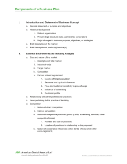

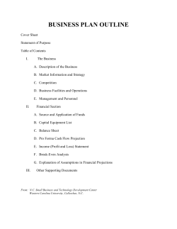


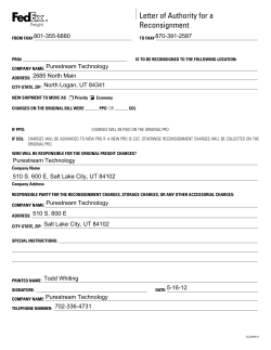
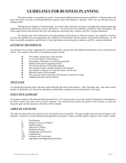


© Copyright 2026