1. science
2. mathematics
3. algebra

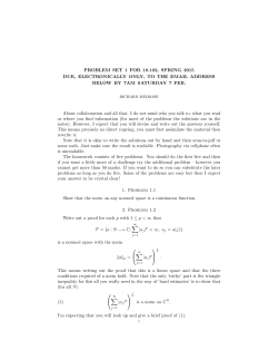
Regularity of BPA-Systems is Decidable
Sjouke Mauw and Hans Mulder
Dept. of Mathematics and Computing Science,
Eindhoven University of Technology,
P.O. Box 513, 5600 MB Eindhoven, The Netherlands.
[email protected], [email protected]
Abstract. It is decidable whether a system in Basic Process Algebra
(BPA) is regular with respect to bisimulation semantics. Basic operators
in BPA are alternative composition, sequential composition and guarded
recursion. A system is regular if the interpretations of all process variables dened in the system have nitely many states. We present an
eective method to transform a BPA specication into a linear specication whenever possible.
1 Introduction
An important issue in automatic verication of concurrent systems using process
algebra is extending the techniques to systems with an innite state space. The
simplest extension of regular specications is BPA (Basic Process Algebra [3]),
which has operators for alternative and sequential composition and allows for the
construction of innite processes by means of guarded recursion. The languages
generated by BPA specications are exactly the context-free languages. However,
we will not study language equivalence, but bisimulation equivalence ([9]) which
is considered more appropriate for verication purposes.
It has already been shown that bisimulation equivalence is decidable for BPA
processes ([1, 4]). An open problem was the question whether it is decidable if
a BPA specication is regular (i.e. whether it can be interpreted as a graph
which has nitely many states). If so, this would enable the application of the
well known algorithms for regular systems to those BPA specications which
are in fact regular. This would help in deciding exactly when to use existing
ecient implementations for deciding bisimulation equivalence (for example for
the PSF-Toolkit [7]).
In this paper we prove that it is decidable whether a BPA system is regular,
that is, all process variables dened by it are regular. Some results for similar specication languages are known. Weakening BPA by replacing the general
multiplication by action prex multiplication will only allow the description of
regular systems, while extending BPA with the communication merge to ACP
(the algebra of communicating processes, [3]) yields a language in which regularity is not decidable. It is also known that regularity of BPA systems modulo
language equivalence is not decidable.
The basic observation in this paper is that if a process is not regular this is
caused by stacking a tail of processes: consider
X = aXb + c
This process can execute a and then enter state Xb. From this state the process
can do an a again and enter state Xbb. Executing more a steps leads to innitely
many dierent states.
In this paper we will formulate the conditions under which this stacking leads
to an irregular process. Furthermore, we give a method to generate a linear
specication if the BPA specication is known to be regular.
This paper is built up as follows. In Sect. 2 we introduce BPA and its interpretation in the graph model. Normed processes and the reachability relation
play an important role in the decision procedure. They are dened in Sect. 3.
Section 4 contains the main theorem of this paper and in Sect. 5 we give a linearization procedure.
Thanks are due to Felix Croes who was of great help while developing the
ideas in this paper and to Michel Reniers for proofreading.
2 Basic Process Algebra
In this section we will give the signature of the theory BPA and its interpretation
in the graph model. For a more detailed treatment we refer to [2].
2.1 Specications
We consider a nite set of atomic actions A. Typical elements of A are a, b, : : : .
Let V be a countably innite set of process variables. Typical elements of V are
X , Y , : : : . A BPA term (over A and V ) is a term constructed from A, V and the
operators and + (sequential and alternative composition). An equation is an
expression of the form X = t, where X 2 V and t is a BPA term. An equation
X = t is guarded if every occurrence of a variable in t is in the sub-term q of some
sub-term p q of t (p, q BPA terms). A (BPA) specication is a nite collection
of guarded equations, such that all variables occurring in the right-hand side of
an equation occur in the left-hand side of some equation and no variable occurs
in the left-hand side of two equations. The collection of variables occurring in
specication S is denoted by VS . If X is a variable dened in S , then Def S (X )
is the right-hand side of the equation of which X is the left-hand side.
If V is a collection of variables, then V denotes the set of all nite sequences
over V . The empty sequence is denoted by . The length jj of a sequence is dened in the usual way. Greek letters , , : : : range over V . Every nonempty sequence of variables can be considered as a BPA term by inserting the
sequential composition operator. If the meaning of a sequence is clear from the
context, we will not explicitly apply conversion functions from sequences to BPA
terms and back. Furthermore if p is a BPA term, the expressions p and p are
interpreted as the BPA term p. Concatenation of sequences and is denoted
by . We have = = .
A specication is in Greibach Normal Form (GNF) if the right-hand sides of
all equations have the form a0 0 + : : : + an n (n 0). Note that i may be so ai i = ai . Given an equation X = a0 0 + : : : + an n , we say that ai i
(0 i n) is a summand of X , notation ai i X .
In [1] it is shown that every BPA specication can be transformed into a
specication in GNF. Therefore we can restrict ourselves to specications in
GNF.
A specication is linear if every summand of every equation in the specication has the form a or a X .
2.2 The Graph Model
We will interpret BPA specications in the so called graph model. This model
consists of nitely branching rooted graphs with labeled edges. This means that
one node is marked as the root and that every edge has a label from a given set
A. A node is a termination node if it has no outgoing edges. A node is also called
a state and an edge a transition.
If there is an edge with label a from node s to
a t, or simply s!t. If there is a sequence of edges
node t, we denote this by s!
a0 s : : : a!
n?1
!n?1 sn , or simply s0 ! sn .
sn (n > 0) then we write s0 a0 :::a
s0 !
1
Denition 1. A relation R between the nodes of two graphs g and h is a bisimulation if the following holds.
{ If s!a s0 is an edge in g and R(s; t), then there is an edge t!a t0 in h such that
R(s0 ; t0 ).
{ If t!a t0 is an edge in h and R(s; t), then there is an edge s!a s0 in g such that
R(s0 ; t0 ).
Two graphs g and h are bisimilar, notation g$
{{ h, if there is a bisimulation
relating the roots of g and h.
The collection of graphs divided out by bisimulation equivalence is denoted
by G=$
{{ . This is a model of BPA. The notion of bisimulation can easily be
extended to nodes from the same graph. For details see [2].
A specication in GNF is interpreted in G=$
{{ in the following way.
Denition 2. Let S be a specication and
2 VS , then gr S () is the graph with
a
nodes VS , root node and edges fX ! j a 2 A; X 2 VS ; ; 2 VS ; aX g
From this denition it follows that is the only termination node. This
construction is equivalent to the standard interpretation of BPA terms in the
graph model. The above denition satises our needs in the easiest way. For
; 0 2 VS we say that and 0 are bisimilar, notation $
{{ 0 , if gr S () and
0
gr S ( ) are bisimilar.
Proposition 3. Let S be a specication and ; 0 ; 2 VS
1. ! 0 ) ! 0 2. =
6 ^ 6= ^ ! ) ! ^ ! a 0 ) !
a 0 , which
Proof. 1. From the denition of the edges we infer !
can be generalized using induction on the number of transitions.
2. Proof by induction on the number of transitions in the sequence ! . If
! in one step, then either or equals . If !1 : : : ! in n + 1
steps, either = , in which case the implication is trivially true, or is of
the form X , where X has a summand a and 1 = . Now there are two
cases. The rst case is = . Then ! and = 1 ! in n transitions.
The second case is 6= , then we can apply the induction hypothesis to
and .
ut
Denition 4. A graph is regular if it is bisimilar to a graph with a nite set
of nodes. Let S be a specication and X 2 VS , then X is regular if gr S (X ) is
regular. A specication is regular if all variables in VS are regular.
Two alternative characterizations of regularity follow directly from the denition.
Proposition 5. (i) A graph is regular if and only if there is no innite sequence
s !s !s ! : : : such that si$
{6 { sj for i 6= j , where s is the root of the graph. (ii)
A graph is regular if and only if there is no innite sequence s ! s ! s ! : : :
6 j , where s is the root of the graph.
such that si$
{6 { sj for i =
0
1
2
0
0
1
2
0
Refer to [8] for a proof of the following proposition, which gives a correspondence between regular and linear specications.
Proposition 6. A specication S is regular if and only if there is a linear specication T such that VS VT and for all X 2 VS gr S (X )$
{{ gr T (X ).
3 Normed Processes and the Reachability Relation
3.1 Normed Processes
A weakly normed process (or normed process for short) is a process which may
terminate in a nite number of steps.1
Denition 7. A node s in a graph is normed, notation s#, if s is a termination
node, or there is a termination node t such that s! t. A node that is not normed
is called (strongly) perpetual , notation s*. A graph is normed if its root node
is normed. If S is a specication and 2 VS then we say that is normed if
2
gr S () is normed.
1
A strongly normed process is a process which may terminate at any point during its
execution. We will not use this notion in this paper.
2
A process is called weakly perpetual if it is not strongly normed.
Proposition 8. Let S be a specication and ; 2 VS then
# , # ^ #
Proof. If or is a termination node, and thus equal to , the proposition
is clearly true. Now suppose ! and ! , then use Proposition 3.1 to derive ! . For proving the other implication, suppose ! then we can use
Proposition 3.2 to derive ! and ! .
ut
Proposition 9. Let ; 2 VS such that *, then gr S ()$
{{ gr S ().
Proof. Construct a bisimulation by relating to for all ; 2 VS for which is perpetual.
ut
In a given state, we can count the minimal number of transitions needed to
terminate. This is called the norm of the state.
Denition 10. The norm of a node s is inductively dened by
8
if s*
<1
if s# and s is a termination node
norm (s) = : 0
1 + minfnorm (t)js!tg if s# and s is not a termination node
Proposition 11. For all nodes s and t s$
{{ t implies norm (s) = norm (t).
Proof. If both s and t are perpetual, then it is clear. Because s and t are bisimilar,
it is impossible that s is perpetual and t is normed or vice versa. If s and t are
normed, use induction on the norm.
ut
Given a specication S we can calculate the normed variables in the following
way. Dene a sequence of sets of variables Ni inductively by
N0 = ;
Ni+1 = Ni [ fX j 9aX;2VS 8Y 2 Y 2 Ni g
Now set N = [i0 Ni then N can be computed eectively.
Theorem 12. The set N contains exactly all normed variables of VS . There is
some i 0 such that Ni = Ni+1 and for this value N = Ni .
Proof. It is clear from the construction that N contains only normed variables.
In order to see that N contains all normed variables, we suppose that X is the
variable such that X #, X 62 N and X ! with a minimal number of transitions.
We consider two cases. If X !, then X has a summand a for some a 2 A and
thus X 2 N1 , which is a contradiction. If X !X0 : : : Xn ! , then (X0 : : : Xn )#
and thus X0 ! , : : : Xn ! . These variables all need at least one less transition
to reach than X , so they are elements of N . But by the denition of N this
would imply that X 2 N , which again gives a contradiction.
Finally, since the Ni are an increasing sequence of subsets of VS and VS is
nite, there are only nitely many dierent sets Ni and therefore there exists an
i such that Ni = Ni+1 , which implies that Ni+k = Ni for all k.
ut
If we dene n + 1 = 1 + n = 1 we have the following proposition.
Proposition 13. For ; 2 VS norm () = norm () + norm ()
Proof. Induction on the length of . If = or = then it is clearly true. If
= X0 then norm (X0 ) = norm (X ) + norm (0 ) = norm (X ) + norm (0 ) +
norm () = norm (X0 ) + norm (). The rst equality can be proven with induction on the norm of X .
ut
Proposition 14. Let X 2 VS , ; 2 VS, then
# ^ X ! ) X ! Proof. From # we derive = or ! . In the rst case the proposition is
trivially true, In the second case we can use Proposition 3.1 to get ! and
by transitivity X ! .
ut
3.2 Reachability
The reachability relation X ,!
Y expresses that variable X can become variable
Y after executing a number of transitions. The sequence is stacked after Y
and will be executed upon termination of Y .
Denition 15. Let S be a specication, then we dene the reachability relation
,!S on VS VS VS for all X; Y 2 VS ; 2 VS by
X ,!
S Y , 92VS ;a2A aY X ^ #
We will write ,! instead of ,!S if S is known from the context.
0 1
X1 ,! : : :
Denition
16. Consider for n > 0 the reachability sequence X0,!
n?1
,! Xn , then we dene the following properties
1. The sequence is normed if (Xn n?1 : : : 0 )#.
2. The sequence is a cycle if X0 = Xn .
3. A cycle is minimal if 80i<jn Xi = Xj ) i = 0 ^ j = n
4. The sequence is stacking if n?1 : : : 0 6= .
Since VS is nite, we can consider (VS ; ,!S ) as a nite graph and thus we
have the following proposition.
Proposition 17. For a given specication S , ,!S has nitely many minimal
cycles.
Reachability implies a transition relation:
Proposition 18. For all X; Y 2 VS ; 2 VS
X ,!
Y ) X! Y a Y . Since is normed,
Proof. Suppose X ,!Y , then aYX which gives X !
we can use Proposition 14 and conclude X ! Y.
ut
0
: : : ,n!?1 Xn (n > 0) is a reachability sequence, then
Corollary 19. If X0,!
X0 ! Xn n?1 : : : 0 .
4 Deciding Regularity
Theorem 20. A specication S is regular if and only if ,!S has no normed
stacking minimal cycles.
Proof. First we prove the \only if" part by contradiction. Suppose that ,!S
0 n?1
has a normed stacking cycle X ,!
: : : ,! X (n > 0), then from Corollary 19 we
conclude X ! X, where = n?1 : : : 0 . Since the cycle is stacking, 6= .
Using Proposition 3.1 we can construct a sequence
X ! X! X! X! : : : :
We calculate the norm of each state using Proposition 13:
norm (Xi ) = norm (X ) + i norm ()
The cycle under consideration is normed, therefore (X)#, therefore X # and #
(Proposition 8). In other words, norm (X ) < 1 and norm () < 1. Moreover,
the cycle is stacking, hence norm () > 0. Consequently, for i 6= j , norm (Xi ) 6=
norm (Xj ). Using the fact that bisimulation respects the norm (Proposition 11)
we have Xi$
{6 { Xj and thus S is not regular (Proposition 5.ii).
The \if" part of the proof is more elaborate. Assuming that some X 2 VS is
not regular, we derive a contradiction. By Proposition 5.i there exists an innite
sequence (setting 0 = X )
0 !1 !2 ! : : :
such that i$
{6 { j for i; j 0, i 6= j . From the absence of normed stacking cycles,
we will derive the existence of i and j (i 6= j ) such that i $
{{ j and thus we will
have a contradiction.
The rst step is to make the relation between the individual variables from
i and i+1 explicit. For this purpose, we will consider the innite sequence as
a directed tree with labeled nodes and unlabeled edges. For every variable in i
(i 0), we create a node. This node is related to all reachable successors (if any)
of this variable in i+1 . Formally:
Denition 21. For every i 0 we have nodes hi; 0i, : : : , hi; ji j ? 1i. The label
L(hi; ki) of node hi; ki is the kth variable of i (if we start counting at 0).
An edge from node hi; pi to node hi + 1; p0 i is denoted by hi; pi;hi + 1; p0 i.
The edges are dened as follows. Let i 0 and i = X : : : Xk (k 0) then,
following Denition 2, the transition i !i is due to a summand aX . Now
0
we consider two cases.
+1
0
1. jj = 0 and thus = . Then i+1 = X1 : : : Xk . For 1 p k we dene
edges from hi; pi to hi + 1; p ? 1i.
2. jj > 0 and thus = Y0 : : : Yh (h 0). Then i+1 = Y0 : : : Yh X1 : : : Xk .
There are two sub-cases.
(a) If # then we dene edges from hi; 0i to all nodes hi +1; 0i, : : : , hi +1; hi.
(b) If * then there is an m 0 such that Ym * and Y0 : : : Ym?1 #. Then we
dene edges from hi; 0i only to the nodes hi + 1; 0i, : : : , hi + 1; mi.
Moreover in both sub-cases we dene edges from hi; pi to hi + 1; h + pi for
1 p k.
This construction implies that the sequence of labels at level i, namely
L(hi; 0i) : : : L(hi; ji j ? 1i) is exactly i . Furthermore, a node hi; pi has exactly
one successor if p > 0, while if p = 0 then hi; pi may have more than one successor
or none at all.
Example 1. Figure 1 below shows a specication and a fragment of the graph
corresponding to the sequence
S !TUV !WXY UV !XY UV ! : : : :
A node hi; ki is represented by its label L(hi; ki) appearing as the kth letter on
the ith line in the gure (counting from 0); arrows denote ; relationships. Note
that the graph is almost a tree; it would be a tree if there were an edge from
h1; 0i (with label T ) to h2; 2i (with label Y ). This edge is omitted because X is
perpetual.
S
T
U
V
W
X
Y
Z
= aT UV
= bW XY + b
=c
=d
=e
= fZX
=g
=h
S
T U V
W X Y U V
X Y U V
Z X Y U V
X Y U V
Fig. 1. Sample specication and successor graph
Before completing the proof of Theorem 20, we will formulate a few lemmas
relating ; to ,!.
Lemma22. If there is an edge hi; pi;hi + 1; qi such that p > 0, then
L(hi; pi) : : : L(hi; ji j ? 1i) = L(hi + 1; qi) : : : L(hi + 1; ji+1 j ? 1i)
ut
Proof. This follows directly from the denition.
Lemma 23. Let n > 0, i 0 and hi; 0i;hi + 1; p i; : : : ;hi + n; pni be a
sequence of edges such that p > 0, : : : , pn? > 0, then there exists 2 VS
such that for all 0 < k n, L(hi; 0i),!L(hi + k; pk i) and L(hi + k; pk + 1i)
L(hi + k; pk + 2i) : : : L(hi + k; ji k j ? 1i) is equal to L(hi; 1i) : : : L(hi; ji j ? 1i).
1
1
1
+
Proof. Induction on n.
If n = 1 then we consider the edge hi; 0i;hi + 1; p1i. Then we have i =
X0 : : : Xk , i+1 = Y0 : : : Yh X1 : : : Xk such that 0 p1 h and aY0 : : : Yh X0 .
Yp +1 :::Yh
Because Y0 : : : Yp1 ?1 #, this gives a reachability step X0 1 ,! Yp1 , and thus
Yp +1 :::Y
L(hi; 0i) 1 ,! h L(hi + 1; p1 i). If we take = Yp1 +1 : : : Yh then L(hi + 1; p1 + 1i)
L(hi + 1; p1 + 2i) : : : L(hi + 1; ji+1 j ? 1i) is equal to L(hi; 1i) : : : L(hi; ji j ? 1i),
because both sequences are Yp1 +1 : : : Yh X1 : : : Xk .
If n = m + 1, then by the induction hypothesis there is a such that for
all 0 < k m, L(hi; 0i),!L(hi + k; pk i) and L(hi + k; pk + 1i)L(hi + k; pk + 2i)
: : : L(hi + k; ji+k j ? 1i) is equal to L(hi; 1i) : : : L(hi; ji j ? 1i). We have an edge
hi + m; pmi;hi + m + 1; pm+1 i, and pm 6= 0, so Lemma 22 applies. This yields
L(hi + m + 1; pm+1i) : : : L(hi + m + 1; ji+m+1 j ? 1i) =
L(hi + m; pmi)L(hi + m; pm + 1i) : : : L(hi + m; ji+m j ? 1i) =
L(hi + m; pmi)L(hi; 1i) : : : L(hi; ji j ? 1i)
The second equality follows from the induction hypothesis with k substituted by
m.
The rst equality implies that L(hi + m + 1; pm+1 i) = L(hi + m; pmi). By the
induction hypothesis L(hi; 0i),!L(hi + m; pmi) and thus L(hi; 0i),!L(hi + m + 1;
pm+1 i).
ut
Corollary 24. Let n > 0, i 0 and hi; 0i;hi + 1; p i; : : : ;hi + n; pni be a
1
sequence of edges such that pv = 0 only for the values v0 , : : : vq of v, then there
exists a reachability sequence L(hi; 0i),!0 L(hi + v0 ; 0i),!1 : : : ,!q L(hi + vq ; 0i), such
that L(hi + vj ; 1i) : : : L(hi + vj ; ji+vj j ? 1i). is equal to q : : : 1 0 L(hi; 1i) : : :
L(hi; ji j ? 1i)
We will say that hj; qi is a descendant of hi; pi if there is a sequence of ;
edges from hi; pi to hj; qi.
Lemma 25. All nodes hn; 0i (n > 0) are descendents of node h0; 0i.
Proof. Suppose hi; pi is not a descendent of h0; 0i, then let j be the smallest
number such that for some q, hi; pi is a descendant of hj; qi. The only sub-case
of Denition 21 where a node does not have a predecessor is the last one, so
L(hj; mi)* for some m < q. Therefore there is some r < p such that L(hi; ri) is
a descendant of L(hj; mi). Hence, p > 0.
ut
Now we complete the proof of Theorem 20. Let T be the subtree formed by all
descendants of node h0; 0i. T must be innite because it contains all nodes hn; 0i
(Lemma 25). T is nitely branching, therefore by Konig's Lemma it contains an
innite branch. Let B be the lowest innite branch, that is, the innite branch
with nodes hi; pi i such that for all i if hi; qi is on an innite branch, then q pi .
Since for every i there is a unique pi such that hi; pi i 2 B , we may consider
B as a function mapping i to pi .
We claim that for innitely many i 0 we have hi; 0i 2 B . Suppose that this
is not the case, then for all n greater than some value k the nodes hn; 0i are not
in B .
Such a node hn; 0i is a descendant of a node hk + 1; j i with j < jj j. Since
there are innitely many such n and nitely many such j , at least one node
hk + 1; j i must have innitely many descendants hn; 0i. That node is therefore
the root of an innite subtree and we apply Konig's Lemma to nd an innite
branch B 0 in this subtree. B 0 can be extended to an innite branch in T , which
contradicts the fact that B is the lowest innite branch.
Now nd the rst j such that there is an i < j with L(hi; 0i) = L(hj; 0i) and
0
:::
hi; 0i,hj; 0i 2 B . By Corollary 24 there is a reachability sequence L(hi; 0i),!
q
,!L(hj; 0i). Since j is minimal, this sequence is a minimal cycle. Moreover,
L(hj; 0i)L(hj; 1i) : : : L(hj; jj j ? 1i) is equal to L(hi; 0i)q : : : 0 L(hi; 1i) : : :
L(hi; ji j ? 1i).
We can repeat this construction, nding the rst j 0 > j such that there is
an i0 satisfying j < i0 < j 0 and L(hi0 ; 0i) = L(hj 0 ; 0i), giving us another occurq0
rence of a minimal cycle L(hi0 ; 0i),!0 : : : ,!
L(hj 0 ; 0i), with L(hj 0 ; 0i)L(hj 0 ; 1i) : : :
L(hj 0 ; jj0 j ? 1i) is equal to L(hi0 ; 0i)q0 : : : 0 L(hi0 ; 1i) : : : L(hi0 ; ji0 j ? 1i).
Repeating this construction innitely often produces innitely many occurrences of minimal cycles. Since there are only nitely many minimal cycles
(Proposition 17), some minimal cycle occurs at least twice. Say X ,!0 : : : ,!q X
with occurrences L(hi; 0i),!0 : : : ,!q L(hj; 0i) and L(hi0 ; 0i),!0 : : : ,!q L(hj 0 ; 0i). Setting = q : : : 0 , we know
L(hi; 0i) = L(hj; 0i) = L(hi0 ; 0i) = L(hj 0 ; 0i) = X ,
L(hj; 0i)L(hj; 1i) : : : L(hj; jj j ? 1i) = L(hi; 0i)L(hi; 1i) : : :L(hi; ji j ? 1i), and
L(hj 0 ; 0i)L(hj 0 ; 1i) : : : L(hj 0 ; jj0 j ? 1i) = L(hi0 ; 0i)L(hi0 ; 1i) : : : L(hi0 ; ji0 j ? 1i)
We consider two cases. First let = , then
L(hj; 0i) : : : L(hj; jj j ? 1i) = L(hi; 0i) : : : L(hi; ji j ? 1i)
and thus i = j which implies i $
{{ j . Thus we have found i and j as promised
at the start of the proof.
The second case is 6= . Since there are no normed stacking cycles and
cycle X ,!0 : : : ,!q X is stacking, it must be a perpetual cycle. This means that *.
Consequently (Proposition 9),
L(hj; 0i)L(hj; 1i) : : : L(hj; jj j ? 1i) =
L(hi; 0i)L(hi; 1i) : : : L(hi; ji j ? 1i)$
{{
L(hi; 0i) =
L(hi0 ; 0i)$
{{
L(hi0 ; 0i)L(hi0 ; 1i) : : : L(hi0 ; ji0 j ? 1i) =
L(hj 0 ; 0i)L(hj 0 ; 1i) : : : L(hj 0 ; jj0 j ? 1i)
and thus j $
{{ j0 , and again we have found i and j as promised. This concludes
the proof of Theorem 20.
ut
5 Linearization
A specication in GNF can be transformed into a linear specication if the conditions from the main theorem in the previous section are met. In this section we
will give an eective linearization method. The idea behind the method is simply
to get rid of anything following a perpetual variable and introduce new process
variables corresponding to sequences of old ones. If this procedure converges, it
yields a linear BPA-specication equivalent to the original one.
First we need some additional denitions.
Denition 26.
1. If is a non empty sequence of variables, then [] denotes a fresh process
variable.
2. If S is a specication, then [S ] is the collection of equations derived from S
by replacing every summand aXY by a[XY ].
3. The operator concatenates a sequence of variables to a process denition.
It is dened as follows.
(a0 0 + : : : + an n ) X = a0 0 X + : : : + an n X
if #
a X = aX
a if *
Denition 27. A specication S is reduced if for every summand aX0 : : : Xn
(n > 0) (X0 : : : Xn?1 )#.
Denition 28. The reduction red (S ) of a specication S is derived from S by
replacing all summands aX0 : : : Xn (n > 0) for which there exists 0 i < n with
(X0 : : : Xi?1 )# and Xi * by aX0 : : : Xi .
A specication S can be linearized by calculating a sequence of equivalent
specications Si (i 0). If S is regular, only a nite number of specications
must be calculated in order to reach a linear Si . The specications are dened
as follows.
S0 = red (S )
Si+1 = [Si ] [ f[XY ] = Def red (S) (X ) Y j
X; Y 2 VS ; 2 VS ; 9a2A;Z 2VSi aXY Z; [XY ] 62 VSi g
We will not present a detailed proof of the correctness of this method. We
will only give the main steps of the proof.
It is easy to verify that every Si is a reduced specication. Furthermore, by
constructing a bisimulation, we have for all X 2 VS and i 0, gr S (X )$
{{ gr Si (X ).
Finally we have that S is regular if and only if for some i 0 Si = Si+1 . We
will only sketch the proof. Suppose that Si = Si+1 , then Si = [Si ], so there are
no summands aXY and thus Si is linear, which implies that S is regular. For
the other implication, suppose that all Si are dierent, then there is an innite
sequence
X !S1 [1 ]!S2 [2 ]!S3 : : :
such that [i+1 ] 2 VSi+1 and [i+1 ] 62 VSi for i 0. This sequence can be
transformed into an innite sequence
X !S 10 !S 20 !S : : :
of which innitely many sequences i0 are not bisimilar. This contradicts regularity of S .
6 Example
We will apply the results from the previous sections to a simple example. Consider the following specication.
A = aBCD
B = bB + b
C = cAC + c
D=d
Clearly the variables B , C and D are normed and since aBCD is a summand
of A, A is normed too. Next we derive a reachability sequence. Since B #, we
D
C
have A,!
C and since A#, we have C ,!
A. Thus we have a reachability cycle
D C
A,!C ,!A. This cycle is clearly stacking, and because ACD# it is a normed
cycle. Now we may conclude that the specication is not regular. Indeed we
have an innite sequence
A! ACD! ACDCD! : : :
Now consider a slightly modied system, which is derived from the previous
system by deleting summand c of C . This makes C perpetual.
A = aBCD
B = bB + b
C = cAC
D=d
The variables B and D are normed, while A and C are perpetual. We can nd
three minimal cycles
B ,!
B
D C
A,!C ,!A
C D
C ,!
A,!C
The rst cycle is not stacking. The second and third cycle (which are in fact
equal) are not normed, because (ACD)* and (CDA)*. Following the main theorem, we conclude that the specication is regular. Now we can apply the linearization procedure and get for S0 the reduction of S :
A = aBC
B = bB + b
C = cA
D=d
For S1 we obtain:
A = a[BC ]
B = bB + b
C = cA
D =d
[BC ] = bBC + bC
Already S2 is a linear specication:
A = a[BC ]
B = bB + b
C = cA
D =d
[BC ] = b[BC ] + bC
7 Conclusions
We have proved that regularity of BPA systems is decidable. The question
whether it is decidable that a single process variable denes a regular process
is still open. We conjecture that it is decidable. A simple example shows that
this question is more complicated than regularity of a complete BPA system.
Consider the specication
X = aY Z
Y = bY c + d
Z = eZ
Then it is easy to show that X and Y are irregular, so the specication as a
whole is irregular. If we would change the denition of Z into
Z = cZ
then the complete specication is still irregular (since Y is still irregular), but
now X is regular. The reason is clearly that the normed stacking tail cn of Y is
reduced to a regular perpetual process c1 by appending Z .
From this example we conclude that it is necessary to take the actual values
of the atomic actions into account when deciding regularity of a single process
variable. This probably leads to a more complex decision procedure than the
one presented in this paper. Since the reachability relation and normedness are
completely independent of the actual atomic actions, only the presence of any
atomic action plays a role in the decision prodedure presented here.
We do not think that the restriction to complete systems is a problem in
practical applications. In most cases one is interested in the linearization of
a complete system. Specications in languages such as PSF [6] only consider
complete systems, without singling out a specic variable.
We claim that the techniques described in this paper easily extend to BPA
(which results from BPA by adding the special process constant for unsuccessful termination). A more interesting topic for future research is the question
whether there are extensions of BPA with some operator for parallelism, on
which regularity is also decidable.
References
1. J.C.M. Baeten, J.A. Bergstra & J.W. Klop, Decidability of bisimulation equivalence for processes generating context-free languages, Proc. PARLE 87 (J.W. de
Bakker, A.J. Nijman, P.C. Treleaven, eds.), LNCS 259, pp. 93-114, 1987.
2. J.C.M. Baeten & W.P. Weijland, Process algebra, Cambridge Tracts in Theoretical Computer Science 18, Cambridge University Press, 1990.
3. J.A. Bergstra & J.W. Klop, Process theory based on bisimulation semantics,
Linear time, branching time and partial order in logics and models for concurrency
(J.W. de Bakker, W.P. de Roever, G. Rozenberg, eds.), LNCS 354, pp. 50-122,
1989.
4. S. Christensen, H. Huttel & C. Stirling, Bisimulation equivalence is decidable for
all context-free processes, Proc. CONCUR'92 (W.R. Cleaveland, ed.), LNCS 630,
pp. 138-147, 1992.
5. S. Christensen, Y. Hirschfeld & F. Moller, Bisimulation equivalence is decidable
for basic parallel processes, Proc. CONCUR'93 (E. Best, ed.), LNCS 715, pp.
143-157, 1993.
6. S. Mauw & G.J. Veltink, A process specication formalism, Fundamenta Informatic XIII, pp. 85-139, 1990.
7. S. Mauw & G.J. Veltink, Algebraic specication of communication protocols,
Cambridge Tracts in Theoretical Computer Science 36, Cambridge University
Press, 1993.
8. R. Milner, A complete inference system for a class of regular behaviours, JCSS
28, pp. 439{466, 1984.
9. D.M.R. Park, Concurrency and automata on innite sequences, Proc. 5th GI
Conf. (P. Duessen, ed.), LNCS 104, pp. 167-183, 1981.
This article was processed using the LaTEX macro package with LLNCS style